GPU-Based High-Performance Imaging for Mingantu Spectral RadioHeliograph

Abstract

As a dedicated solar radio interferometer, the MingantU SpEctral RadioHeliograph (MUSER) generates massive observational data in the frequency range of 400 MHz – 15 GHz. High-performance imaging forms a significantly important aspect of MUSER’s massive data processing requirements. In this study, we implement a practical high-performance imaging pipeline for MUSER data processing. At first, the specifications of the MUSER are introduced and its imaging requirements are analyzed. Referring to the most commonly used radio astronomy software such as CASA and MIRIAD, we then implement a high-performance imaging pipeline based on the Graphics Processing Unit (GPU) technology with respect to the current operational status of the MUSER. A series of critical algorithms and their pseudo codes, i.e., detection of the solar disk and sky brightness, automatic centering of the solar disk and estimation of the number of iterations for clean algorithms, are proposed in detail. The preliminary experimental results indicate that the proposed imaging approach significantly increases the processing performance of MUSER and generates images with high-quality, which can meet the requirements of the MUSER data processing.

1 Introduction

Radio astronomical observation techniques have undergone rapid advancements since Martin Ryle first proposed the use of aperture synthesis imaging for radio astronomy (Ryle, 1962). Modern interferometric instruments ranging from the Expanded Very Large Array (EVLA), the Low Frequency Array (LOFAR), and the Australian Square Kilometre Array Pathfinder (ASKAP) to the world’s largest radio telescope Square Kilometre Array (SKA) are increasingly subject to a data deluge, which poses great challenges to high-performance data processing.

Over the past few years, observations of solar emissions at metric wavelengths have yielded new insights into solar activities such as particle acceleration, coronal mass ejections (CMEs) and flares. The currently available radio telescopes observes the solar at only at a few discrete frequencies: the Nobeyama Radioheliograph (NoRH) makes observations at 17 GHz and 34 GHz, the Nancay Radioheliograph (NRH) operates at 5 – 10 frequencies in the range of 150 – 450 MHz (Kerdraon & Delouis, 1997), the frequency range of Gauribidanur Radioheliograph is 40 – 150 MHz, and the Siberian Solar Radio Telescope (SSRT) acquires data at 5.7GHz. Meanwhile, large interferometers such as the Very Large Array (Napier et al., 1983) and the Westerbork Synthesis Radio Telescope (WSRT) are primarily designed for rotational synthesis observations and their fields of views are typically too small to cover the entire solar disk (Baars et al., 1973; Yan et al., 2015).

The MingantU SpEctral RadioHeliograph (MUSER) is a solar-dedicated interferometric array constructed to investigate the dynamics properties of solar bursts. The MUSER was built at Mingantu in Inner Mongolia, China. The MUSER comprises two sub-arrays: MUSER-I, operating in the frequency range of 400 MHz – 2 GHz with 40 4.5-m antennas, whose observation (covers 1.6 GHz bandwidth, two polarizations) is divided into four bands, and MUSER-II, operating in the frequency range of 2 GHz – 15 GHz with 60 2-m antennas, whose observation (covers 13 GHz bandwidth, two polarizations) is divided into 33 bands. Notice that there are 8 repeated channels among the 528 channels of MUSER-II. The specifications of the MUSER are listed in Table 1 (Yan et al., 2011). The digital receivers can be specified to work in loop mode (loop both in bands and polarizations) or fix mode (fix in one band and one polarization). Every 3 ms, both the digital receivers of MUSER-I and MUSER-II receive 400 MHz analog signals in a specific polarization and the correlators simultaneously output 16 channels with a 25 MHz bandwidth for each channel (Yan et al., 2011; Wang et al., 2015). Therefore, the MUSER is expected to provide a new observational window on solar activities as a new instrument that is capable of operating at hundreds of frequencies and nearly simultaneously generating high-quality radio images with high temporal, high spatial, and high spectral resolutions. (Yan et al., 2004, 2009, 2010, 2011).

Table 1: MUSER Characteristic and Performance

Parameters	MUSER-I	MUSER-II
Antenna array	40 (4.5 meters)	60 (2 meters)
Frequency range	0.4 GHz$-$2.0 GHz	2.0 GHz$-$15 GHz
Frequency resolution	64 channels	520 channels
Channel bandwidth	25 MHz
Time resolution	25 ms	206.25 ms
Spatial resolution	${51.6}^{\prime\prime}-{10.3}^{\prime\prime}$	${10.3}^{\prime\prime}-{1.4}^{\prime\prime}$
Baseline length	$\sim 8m-\sim 3000m$	$\sim 4m-\sim 3000m$
Polarization	Dual circular left and right
Dynamic range	25 db (snapshot)
Field of view	$0.6^{\circ}-7^{\circ}$

Since the successful installation of the MUSER hardware, a series of measurements and experiments has been conducted on the MUSER system (Wang et al., 2013). The phase closure relationship in the experiments reflected the appropriate design of the whole system (Wang et al., 2013). The first radio burst presented by Yan et al. (2015) and the simulation results by Du et al. (2015) demonstrated the imaging capability of the MUSER. Meanwhile, a distributed computing framework, Opencluster, has been designed to meet the requirements of high-performance data processing (Wang et al., 2015; Wei et al., 2016).

However, high-performance imaging is still a critical problem for the MUSER. According to the specific parameters listed in Table 1, both MUSER-I and MUSER-II generate raw observational data frames that include 16 frequencies (one band) with one specified polarization every 3 ms, which implies that 614,400 images need to be generated in 1 min if needed. Although the Graphics Processing Unit (GPU) technology has been used in previous studies (Wang et al., 2015), the performance of the MUSER further needs to be boosted urgently.

In addition, due to certain constraints of the current MUSER system, some specific algorithms should be further studied. For example, as a geosynchronous satellite is used as the only available calibrator source and its phase-tracking accuracy is insufficient, it is required to further correct the phase error in dirty images by detecting the solar disk and moving the disk to the image center.

In this study, we focus on the implementation of the MUSER high-performance imaging procedure, particularly the dedicated processing approaches for the MUSER in its current status. The rest of the paper is organized as follows. In section 2, a review of related work is presented. After presenting a broad overview of the imaging pipeline in section 3, we discuss key steps such as the estimation of the solar disk and sky brightness, solar disk automatic centering and the improved clean algorithm in section 4. The implementation and imaging performance is analyzed in section 5. Section 6 discusses the existing problems, and finally, section 7 concludes the paper along with the presentation of certain aspects of our future work.

2 Related Work

A fundamental theory of radio interferometric imaging is the existence a Fourier transform (3D) between the sky brightness and the visibility data obtained with a radio interferometric array (Thompson et al., 2008; Taylor et al., 1999). In particular, if all the visibility data can be approximately considered to lie on a plane and if the field of view is sufficiently small or the time of observation is sufficiently small (snapshot observations), the computation of the sky brightness can be reduced to a 2D transform (Perley, 1999; Bhatnagar, 1999). Although ignoring the w-term can effectively reduces the load during imaging computing, careful calculation of the phase error caused by it is needed in the general case as which may bring serious phase error in images(Perley, 1999).

In general, gridding, weighting, Fourier transform and dirty image cleaning form the main steps in processing data from the interferometer. Radio antenna arrays typically have non-uniform spacing, which gives them simultaneous access to low and high frequencies, but with sparse sampling in the UV plane. In practice, the data are required to be variously weighted according to their reliability (Sault & Oosterloo, 2007). Further, weighting functions are used for controlling the synthesized beam shape (Perley, 1999; Rau et al., 2009). Different methods of weighting, such as natural weighting, uniform weighting and robust weighting, are used during imaging. Gridding is the convolution of the visibilities with a particular function, which resamples the visibility data at grid points (Thompson et al., 2008) as the fast Fourier transform (FFT) requires the visibilities to lie on a regular rectangular grid.

There is a series of clean algorithms for removing instrumental artifacts in dirty images directly generated from the gridding and FFT steps. In this context, Högbom presented a classic image deconvolution algorithm that was considered a milestone in radio astronomy (Högbom, 1974). Subsequently, many improved clean algorithms have been proposed (Taylor et al., 1999; Thompson et al., 2008). For solar observations, the Steer clean was proposed to solve the problems of failing to restore diffuse features and the excessive computational time of the standard Högbom clean. The Steer algorithm suitably restores complicated brightness structures in daily solar images of the Nobeyama Radioheliograph, consuming only one-tenth the time of the classical Högbom algorithm (Koshiishi, 2003). Although Högbom algorithm can address point sources and extended sources very well, the Steering clean is typically regarded as a more appropriate algorithm for cleaning the dirty image of the Sun.

The processing performance forms another key issue in the data reduction of interferometer. To accelerate the computational speed of the gridding and clean steps, a GPU is widely used for interferometric imaging. A GPU-based approach for gridding makes the w–projection 100 times faster than that of general CPU-based imaging tools (Muscat, 2014). The thread coarsening based on a GPU is applied in MeerKAT (Brederode et al., 2016) to improve the efficiency of the existing convolutional gridding algorithm (Merry, 2016).There is also the GPU-accelerated software simulator OSKAR (Mort et al., 2016), which makes it possible to run large-scale, full-sky simulations of aperture arrays on reasonable timescales, and this simulator can be useful for data processing of the SKA. Obviously, the application of GPU–CUDA (Compute Unified Device Architecture) framework has greatly improved the data processing efficiency, and its use is gradually expected to become a trend in massive astronomical data processing in the future.

In addition to fundamental researches on interferometric imaging, many software packages such as CASA (the Common Astronomy Software Applications) and MIRIAD (Multichannel Image Reconstruction, Image Analysis and Display) have been developed and widely used for interferometric data processing. CASA has been mainly developed by C/C++ and partially supports the message passing interface (MPI) parallel computing environment. The MIRIAD was initially implemented in FORTRAN-77 and miriad-python (Williams et al., 2012) was developed to provide Python programming language to the MIRIAD data reduction system. Nevertheless, to handle the data with self-defined data format and meet the unique characteristics of the MUSER, a lightweight and high-efficiency data processing pipeline with appropriate algorithms is in pressing need.

In summary, imaging is a classical problem for which many algorithms have been proposed previously. However, only a few studies have discussed the interferometric imaging of the Sun and the clean algorithms for extended source. Meanwhile, very few studies have described the implementation of high-performance imaging on a GPU platform in detail, and performance-involved factors such as the detection of solar disk and sky brightness and the determination of the number of iterations for clean algorithms are seldom discussed. These topics merit further study in order to optimize the imaging performance and facilitate further data analysis, particularly for specific radio telescopes such as the MUSER.

3 Imaging Pipeline Design

3.1 Imaging Pipeline

The imaging of the MUSER follows the basic principles of an interferometric telescope. Currently, a data processing pipeline has been designed to automatically process the data from the MUSER. Figure 1 illustrates the complete data processing procedure from the raw data acquisition, abnormal data flagging, phase calibration, UV calculation, imaging and the data storage to data publication.

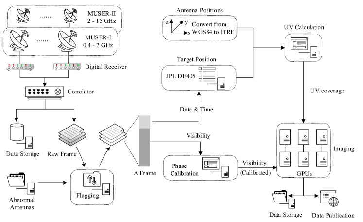
Figure 1: MUSER imaging pipeline.

A series of data pre-processing procedures, i.e., reading the raw data, flagging, and calibration, needs to be performed before imaging. The steps of transmission delay compensation and fringe stopping are performed by the correlator directly, and phase calibration is performed by the geosynchronous satellite as per the MUSER’s current operational status.

To assist the subsequent processing, a lightweight database is created for storing the information of malfunctioning antennas, weather conditions, instrument status and other observation information, which are retrieved during the data processing. An automatic flagging method based on the support vector machine (SVM) is used to flag the visibility data if there is not manual record of malfunctioning antennas (Dai et al., 2017). To accurately calculate the UVW and obtain high-quality dirty images, we implemented a Python package for high-precision target position computing using JPL DE405 Ephemeris, which can meet the accuracy requirements. The imaging process that includes weighting, gridding, FFT and clean steps is executed on a GPU platform. The imaging parameters and key steps are presented in the following sections.

3.2 Imaging Parameters

3.2.1 Image size

The image size forms an important parameter in high-performance imaging. According to the frequency and the longest baseline as per the MUSER design specifications (see Table 1), the spatial resolution should be approximately $51.6{}^{\prime\prime}-10.3{}^{\prime\prime}$ for MUSER-I and $10.3{}^{\prime\prime}-1.4{}^{\prime\prime}$ for MUSER-II, with the corresponding fields of view (FOVs) for non-aliasing being $1.07^{\circ}-5.37^{\circ}$ and $2.15^{\circ}-0.29^{\circ}$ respectively. The final image sizes that required to be generated for different frequencies are listed in Table 2 (three pixels are used to present a spatial resolution). In order to clean an image of a given dimension, it is necessary to have a beam pattern twice as large the image size so that a point source can be subtracted from any point in the map.

Table 2: Imaging size specification

Frequency	Spatial Resolution	Pixel Size	Space Size of Image	Image Size
(GHz)	(arc seconds)	(arc seconds)	(arc minutes)	(pixels)
$0.4-0.6$	$51.6{}^{\prime\prime}-34.4{}^{\prime\prime}$	$17.2{}^{\prime\prime}-11.5{}^{\prime\prime}$	$73.4{}^{\prime}\times 48.9{}^{\prime}$	$256\times 256$
$0.6-1.2$	$34.4{}^{\prime\prime}-17.7{}^{\prime\prime}$	$11.5{}^{\prime\prime}-5.9{}^{\prime\prime}$	$98.1{}^{\prime}\times 50.3{}$’	$512\times 512$
$1.2-2.0$	$17.7{}^{\prime\prime}-10.3{}^{\prime\prime}$	$5.9{}^{\prime\prime}-3.4{}^{\prime\prime}$	$100.7{}^{\prime}\times 58.0{}^{\prime}$	$1024\times 1024$
$2.0-4.0$	$10.3{}^{\prime\prime}-5.2{}^{\prime\prime}$	$3.4{}^{\prime\prime}-1.7{}^{\prime\prime}$	$72.5{}^{\prime}\times 36.3{}^{\prime}$	$1280\times 1280$
$4.0-8.0$	$5.2{}^{\prime\prime}-2.6{}^{\prime\prime}$	$1.7{}^{\prime\prime}-0.9{}^{\prime\prime}$	$72.5{}^{\prime}\times 38.4{}^{\prime}$	$2560\times 2560$
$8.0-15.0$	$2.6{}^{\prime\prime}-1.4{}^{\prime\prime}$	$0.9{}^{\prime\prime}-0.5{}^{\prime\prime}$	$76.8{}^{\prime}\times 42.7{}^{\prime}$	$5120\times 5120$

3.2.2 UVW Calculation

As all antenna positions in the MUSER are measured with the use of the Global Positioning System (GPS), which is based on the World Geodetic System WGS84, it is essential to convert this set of coordinates to International Terrestrial Reference Frames (ITRFs) before computing of the baseline vectors. The geographic coordinates of the Mingantu observational station (longitude=115.2505^∘, latitude=42.211833333^∘, altitude=1365.0 meters) are used during the coordinate conversion. The variations in Earth’s orientation as obtained from the IERS are also considered. The UV coverage of the MUSER is shown in Figure 2.

To eliminate the effects of w-term in MUSER, we chose the implementation of w-projection (Muscat, 2014) which can be run on GPU environment. It should be pointed out, the correction of w-term is determined by the phase error caused by ignoring the w-term, which is defined as $\left|\pi(l^{2}+m^{2})w\right|\ll 1$, where $(l^{2}+m^{2})$ is the synthesized field. When the phase error is small enough, we do not need to correct the w-term so as to improve the performance. A thorough analysis of the w-term is given in section 6.1.

Figure 2: UV coverage of MUSER. (a) UV coverage of MUSER-I on 2015-11-01 at 04:08:49.354161240 (UTC), frequency: 1.7125GHz, polarization: right. (b) UV coverage of MUSER-II on 2016-07-05 at 04:01:38.459449240 (UTC), frequency: 4.1875GHz, polarization: right.

3.2.3 Gridding convolution function

In order to use the FFT transform to improve the imaging performance, the measured visibility must be gridded into a 2D array. For smoothing and interpolating the data, the visibility data are convolved with a suitably chosen gridding convolution function (GCF) before resampling with different weighting methods. In practice, the precise manner in which this is carried out can greatly affect the macroscopic properties of the resulting image, such as both aliasing from the sidelobes and uniform spacing of the grid (Schwab, 1984). Many functions, such as the pillbox, exponential, sinc and spheroidal functions, can be considered for use as the the convolution function. The spheroidal function is used in MIRIAD software (Sault et al., 1995), and as per Schwab’s choice of the optimal gridding method, the spheroidal function was considered as the optimal GCF.

To implement the pipeline, we compared many GCFs and finally selected the truncated spheroidal function with default coefficients listed as per the study of Schwab (1984) for the MUSER data gridding. That is, the visibility is convolved with a spheroidal wave functions and then gridded (uniform and natural weighting are implemented). Inverse FFT is performed after gridding for generating dirty image. The dirty images of the MUSER are shown in Figure 3. The dirty image from a single frame of MUSER-I is presented in Figure 3 (a)) and Figure 3 (b) depicts a 10-min-integrated output of MUSER-II, which can effectively improve the signal-to-noise ratio (SNR).

Figure 3: (a) Dirty image from MUSER-I on 2015-11-01 at 04:08:49.354161240 (UTC) at frequency: 1.7125GHz, polarization: right. (b) 10-min-integrated dirty image from MUSER-II on 2016-07-05 at 04:04:38.459449240 (UTC) to 2016-07-05 04:15:00 (UTC) at frequency: 4.1875GHz, polarization: right.

4 Improved clean algorithm

In the current MUSER data processing system, the Steer clean algorithm is used to clean the dirty image. Obviously, the application of the clean algorithm is a time-consuming iterative processes. It is necessary to estimate the probable number of iterations to improve the clean performance, rather than depending on prior experiential estimates or a given upper limit. Moreover, as can be observed from the dirty images (Figure 3), there is a phase error leading to the solar disk being located off-center in the current stage, which will also affect the subsequent data processing steps such as P-angle correction.

Figure 4 presents the improved clean process. We add a “pre-clean” procedure to detect the solar disk and sky brightness and then carry out the phase correction. Imaging and the improved clean are subsequently performed to obtain clean images.

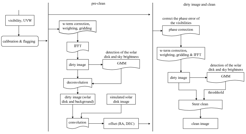
Figure 4: Flowchart showing imaging and clean processes for the MUSER.

4.1 Detection of Solar Disk and Sky Brightness

Theoretically, there are the sky background, solar disk area and solar activity area (if there is solar activity) in the dirty image, and the brightness of these areas differs distinctly. Through analysis, the judgment of different regions reduces to a clustering problem, and data points within the same group can be modeled by a Gaussian distribution. A classical algorithm for classification and modeling, the Gaussian mixture model (GMM) (Ivezić et al., 2014; Wright et al., 2015) is used in our study.

For estimating the solar disk and brightness, the data from a dirty image is divided into 2000 ranges. The histogram in Figure 5 depicts the probability of data points in the corresponding range (considering the dirty image of MUSER-I in Figure 3 as an example). GMM is performed to estimate the parameters of the potentially included Gaussian distributions in the histogram and the results are plotted in Figure 5. According to the brightness of different areas, $\mu$ in curve (a) denotes the maximum likelihood brightness of the sky brightness and $\mu$ in curve (b) indicates the brightness of the solar disk, and this result will be used during the clean processing.

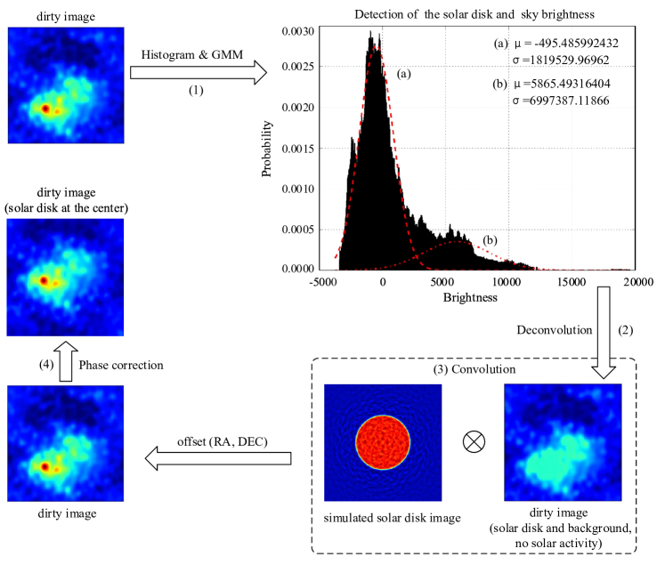
Figure 5: Process of detecting the solar disk and sky brightness and phase correction (pre-clean), considering the dirty image of MUSER-I as an example.

4.2 Disk Centering Correction

After obtaining the estimated solar disk and sky brightness, we follow three steps for disk centering correction:

1. To ensure that there is no solar activity in the dirty image and to acquire more precise offset parameters, deconvolution is performed on the original dirty image until the brightness is equal or lesser than the estimated solar disk brightness (i.e., $\mu$ in curve (b)) from the GMM. This deconvolution processing ensures that the dirty image contains only the solar disk and sky background.

2. A correlation operation is performed between the dirty image in step (1) and the simulated solar disk to obtain the center offset values (i.e., RA offset and DEC offset).

3. The phase of the visibility data is corrected by the RA offset and DEC offset. Figure 5 illustrates the process of this correction.

4.3 Clean with determined number of iterations

In view of the specific characteristic of solar imaging and referring to NoRH, we use a modified deconvolution algorithms, i.e., the Steer clean algorithm, to clean the dirty image acquired with the MUSER. As the number of clean subtractions and the loop gain ($\gamma$) determine the depth of the clean operation (Taylor et al., 1999), which affects the image quality and imaging performance, it is crucial to optimize the loop gain and number of iterations. In this regard, the results of Very Large Array applications suggest that the reasonable compromise range of the loop gain is $0.1\leq\gamma\leq 0.25$ (Taylor et al., 1999). Through experiments, $\gamma=0.1$ is chosen as the optimal loop gain. For the deconvolution, the estimated sky brightness (i.e., $\mu$ in Figure 5 curve (a): $\mu_{a}$) is used as a threshold to automatically determine the number of iterations. That is, the iteration stops when the brightness of the sky is reached.

5 GPU-based imaging implementation and performance

CUDA is a GPU programming model developed by NVIDIA, and it provides a programming interface to utilize the highly-parallel nature of GPUs and mask the complexity of controlling GPUs. For the MUSER data processing, the data preparation is carried out in the CPU environment, and here, we focus on the computation-intensive processes such as gridding, FFT and clean, which are accelerated with the use of GPUs. Algorithm 1 below describes the improved clean process. The clean images are shown in Figure 6 together with the images from NoRH as a comparison.

All the codes used in our study is available at https://github.com/astroitlab/museros. Python is used as the programming language as it is prevalent in astronomical data processing. More importantly, it’s really convenient to use packages such as PyCUDA and Scikit-CUDA, which provide the access to the CUDA parallel computation application programming interface (API). The performances achieved for various key steps are listed in Table 3, considering two representative image sizes as an example. The elapsed time of Steer clean is indicated for one iteration, and the number of iterations for cleaning the dirty images in Figure 3 (a) is 39 and 33 for Figure 3 (b). That is, the total time for generating a dirty image is about 0.26 seconds for MUSER-I and 0.8 seconds for MUSER-II, and for Steer clean, a further about 1.138 s is needed for MUSER-I and 1.45 s is needed for MUSER-II.

Figure 6: (a) Clean image from MUSER-I on 2015-11-01 at 04:08:49.354161240 (UTC), frequency: 1.7125 GHz, polarization: right. (b) 10-mins-integrated clean image of MUSER-II from 2016-07-05 04:04:38.459449240 (UTC) to 2016-07-05 04:15:00 (UTC), frequency: 4.1875GHz, polarization: right. (c) Clean image from Nobeyama on 2015-11-01 at 04:10:00 (UTC), frequency: 17 GHz (R+L). (d) Clean image from Nobeyama on 2016-07-05 at 04:10:02 (UTC), frequency: 17 GHz (R+L)

6 Discussion

The imaging pipeline presented in this study meets the requirements of automatically processing the massive observational data from the MUSER in the current stage. However, there are still some issues that need to be further discussed.

6.1 w-term

W-term is an inevitable problem in the MUSER data processing. Actually, the MUSER has the specifications of small antenna apertures, long baselines and long wavelengths. Therefore, the non-coplanar baselines effect has to be considered so as to obtain high quality observational results.

According to the previous studies (Thompson et al., 2008), w-term may be ignored and a two-dimensional Fourier transform can be used when the term $2\pi w(\sqrt{1-l^{2}-m^{2}}-1)$ is much less than unity. If the antennas track the source under observation down to low elevation angles, the values of $w$ can approach the maximum spacings that is approximately the maximum length of baseline. The the maximum value of the term is expressed as $\frac{B\lambda}{D^{2}}$, where B is the length of baseline, $\lambda$ is the wavelength and $D$ is the antenna diameter. For the observation of the MUSER with 450 MHz and the maximum baseline length of 3000 meters, the value of w-term would be 140.625, which is much larger than unity. Obviously, w-term needs to be more explicitly dealt with or the operation of the instrument will be greatly restricted.

1:Visibilities and UVW (Phase corrected, Flagged)

2:weighting mode: $weight\_mode$, natural or uniform

3:clean images

4:function void $wgtGrid\_kernel$(float2 *Grd, int *cnt, int nu, int mode)

5:     int iu = blockDim.x*blockIdx.x + threadIdx.x;

6:     int iv = blockDim.y*blockIdx.y + threadIdx.y;

7:     int u0 = 0.5*nu; $\triangleright$ Applying the weight to half the grid (as the data is Hermitian)

8:     if $(iu>=u0\&\&iu<nu\&\&iv<nu)$ then

9:         if $(cnt[iv*nu+iu]!=0)$ then

10:              int ind = iv*nu+iu;

11:              float foo = cnt[ind];

12:              float wgt;

13:              if (mode == 1) then

14:                  wgt = 1./foo; $\triangleright$ Uniform Weighting

15:              else

16:                  wgt = 1; $\triangleright$ Natural Weighting               

17:              Grd[ind].x = Grd[ind].x*wgt;

18:              Grd[ind].y = Grd[ind].y*wgt;               

19:

20:function dirty_image($visibilities,UVW,weight\_mode$)

21:     W-term correction (w-projection);

22:     Calculating the weight and gridding: $wgtGrid\_kernel$;

23:     Invert Fast Fourier Transform to get the dirty image, with the sun disk at the center;

24:     return dirty image, dirty beam and clean beam: $gpu\_dirty$, $gpu\_dpsf$, $gpu\_cpsf$;

25:

26:function pre_clean($disk\_model,dirty\_image$) $\triangleright$ Obtaining the phase errors

27:     Apply GMM to a dirty image ($dirty\_image$) and get the estimated solar disk and sky brightness;

28:     Picking out points with brightness-values greater than the estimated solar disk in the dirty image: h_dirty;

29:     Calculating the offset parameters using the the disk model and the h_dirty: $sun\_disk\_offset(disk\_model,h\_dirty)$;

30:     return ra_offset, dec_offset;

31:

32:function improved_clean($dirty\_image,band,channel$)

33:     Obtaining the phase error: (ra_offset, dec_offset) = $PRE\_CLEAN()$;

34:     Phase correction: correct the phase error of the visibility data;

35:     Generating the dirty image: $DIRTY\_IMAGE()$;

36:     Find the strength and position of the peak in the dirty map: ($imax$, $gpu\_max\_id$);

37:     while $imax>\mu_{a}$ do $\triangleright$ loop until: $imax$ (the maximum brightness) $\leq\mu_{a}$ (the sky brightness)

38:         Steer clean;

39:         Find the strength and position of the peak in the dirty map: ($imax$, $gpu\_max\_id$);      

40:     return clean images;

Algorithm 1 MUSER Clean

Table 3: Elapsed time of key steps in MUSER imaging

Subtask No.	Subtask	Frequency/Pixel	Elapsed time (s)
1	Data preparation	0.4 GHz - 2.0 GHz	0.06161
	(Calibration and flagging)	2.0 GHz - 15 GHz	0.13885
2	Gridding, weighting and FFT	1024$\times$1024	0.20664
		2560$\times$2560	0.66279
3	Detection of solar disk and sky brightness	1024$\times$1024	0.44671
	(GMM)	2560$\times$2560	0.46264
4	Phase correction	1024$\times$1024	0.01773
		2560$\times$2560	0.02987
5	Pre-clean	1024$\times$1024	0.67108
	(Subtask 2+3+4)	2560$\times$2560	1.15530
6	Steer clean	1024$\times$1024	0.01773
	(One iteration)	2560$\times$2560	0.02987
7	Generating dirty image	1024$\times$1024	0.26825
	(Subtask 1+2)	2560$\times$2560	0.80164
8	Generating clean image	1024$\times$1024	3.21551
	(Subtask 1+2+3+5+6*NOI)	2560$\times$2560	4.85529

Note. — NOI: Number of iterations. Testing environment: Intel(R) Xeon(R) CPU, 6 cores, 2.10GHz. GPU: NVIDIA Corporation GM200.

In general, the w-term can be ignored when $\left|\pi(l^{2}+m^{2})w\right|\ll 1$. We can possibly allow it to be as high as 0.1 radian without introducing serious errors in the image (Taylor et al., 1999). The observational target of the MUSER is the Sun and the radius of the Sun is about $32^{\prime\prime}$, that is, $(l^{2}+m^{2})$ can be roughly $256^{\prime\prime}$. To guarantee the valid of the equation, the value of the $w$ must be less than 1504.3 (unit: number of wavelength). Obviously, for the observation with different frequency and different target position, we have to calculate the value of the w-term and finally determine the correction of the w term. If the value of the $w$ is less than 1504.3, the correction is not necessary.

We finally realize that the corrections for the w-term is necessary for the MUSER in most cases (about more than 300 days in a year). We calculated the values of w-term at 12:00 am (China Beijing time) every day in the year of 2017 respectively. The maximum value of the w-term (about 2821.55, unit: number of wavelength) in a year appeared on Dec 11 instead of the winter solstice. The minimum value (only 0.000357) of the w-term is on Jun 30. Even on the best day (Jun 30) in a year, only the data in four hours (10:10 am - 14:10 pm) can be directly processed without w-term correction.

6.2 Calibration

.

Calibration is one of the most important issues in interferometric imaging. Currently, two new 20-m diameter antennas are under construction and they are to be used for calibration in the near future. Prior to application of these antennas, we have no effective approach to calibrate the phase and amplitude errors accurately. To ensure that the MUSER generates scientific results as early as possible, a satellite is used to calibrate phase error in the current stage.

Simulations in our previous work proved that the observed image appears a translation when the satellite is subject to position errors. That’s to say, the phase error that leads to the deviation of the solar disk is caused by the pointing error of the satellite. Therefore, it is necessary to further correct the phase error in the pre-clean processing step in the current stage. Current data processing procedure has no absolute calibration with respect to amplitude, scientists can use these data to carry out their scientific research in other specific fields as well.

6.3 Performance and Deployment

From Table 3, we note that the current data processing affords satisfactory performance with the use of GPU technology. we note that the elapsed time of generating a dirty image of 1024$\times$1024 is about 0.268 seconds and 0.8 seconds for a 2560$\times$2560 dirty image.

Full image processing involving dirty image generation, pre-clean and Steer clean would take about 3.22 seconds for a 1024$\times$1024 image and 4.86 seconds for a 2560$\times$2560 image with the use of one machine with one GPU card. Significantly, the comparison experiments of generating clean image using CASA by processing UVFITS file of the MUSER show that the performance of Steer clean based on GPU technology is about 2–8 times faster than the CASA software package, and this performance advantage becomes more obvious especially in processing the data of MUSER-II.

The data processing pipeline has been deployed both for routine observational monitoring and scientific data processing of the MUSER. For real-time monitoring, the aforementioned distributed data processing framework – Opencluster is used to schedule the pipeline on a high-performance CPU/GPU cluster. The current monitoring system could produce 16 cross-correlograms, 16 spectrum diagrams and 16 dirty images of one band in every 5 seconds for MUSER-I and MUSER-II respectively. The performance is enough for the requirements of real-time monitoring.

For the requirement of the scientific data processing, not all observational data would be processed. The pipeline has also been integrated into a command line system, which is convenient for post data processing as it can operate separately on a single machine. In common, the scientists would process the data at a specific time according to their research goal. According to Table 3, the current data processing system can already generate high-quality images with a high-performance.

6.4 Limitations

Detecting the solar disk and sky brightness is indispensable for automatically determining the number of iterations and optimizing the clean performance. However, the current approach strongly depends on the signal-to-noise ratio (SNR) of the image.

According to the results of data processing, the proposed approach of detecting the solar disk and sky brightness is well-suited for high-SNR images because the peak position in the histogram could be correctly recognized. Therefore, this approach is to a certain extent limited for processing snapshot observational data (3 ms/frame) especially in the data processing of MUSER-II.

In addition, a high-performance CPU/GPU cluster is indispensable to process the massive data generated by the MUSER. The current performance level can meet the requirements of a monitoring system which refresh the observational results in every 5 seconds. However, the power consumption needs to be considered because the power supply for a distant observational station is limited.

7 Conclusions and Future work

We optimized and implemented a high-performance data processing pipeline for the MUSER in this study. The preliminary imaging results prove the feasibility of the proposed processing approach. We specifically draw attention to the phase correction in current status and the detection of the solar disk and sky brightness based on the Gaussian mixture model, which automatically determines the number of iterations for clean algorithms. More importantly, the performance of Steer clean based on GPU is far better than the commonly used CASA software.

We have already begun studies on new imaging algorithms such as compressed sensing and so on. Meanwhile, to further improve the imaging quality, it is necessary to further study effective flagging methods, visibility integration, calibration and clean algorithms.

Actually, as same as other new telescope systems, the construction of the MUSER is a long-term effort. The proposed approaches accelerated the scientific data output of the MUSER. Regardless of limitations of the current MUSER operation, we believe that the scientific output of the MUSER is promising and that the MUSER can significantly contribute to astronomical observations in the near future.

References

- Baars et al. (1973) Baars, J. W., van der Brugge, J. F., Casse, J. L., et al. 1973, Proceedings of the IEEE, 61, 1258
- Bhatnagar (1999) Bhatnagar, S. 1999, Notes from summer school on low frequency astronomy at NCRA, Pune
- Brederode et al. (2016) Brederode, L. R., van den Heever, L., Esterhuyse, W., & Jonas, J. L. 2016, in SPIE Astronomical Telescopes Instrumentation, International Society for Optics and Photonics, 990625–990625
- Dai et al. (2017) Dai, H.-m., Mei, Y., Wang, Weiand Deng, H., & Wang, F. 2017, Chinese Astronomy and Astrophysics, 41, 125
- Du et al. (2015) Du, J., Yan, Y., Wang, W., & Liu, D. 2015, Publications of the Astronomical Society of Australia, 32, e024
- Högbom (1974) Högbom, J. 1974, Astronomy and Astrophysics Supplement Series, 15, 417
- Ivezić et al. (2014) Ivezić, Ž., Connolly, A. J., VanderPlas, J. T., & Gray, A. 2014, Statistics, Data Mining, and Machine Learning in Astronomy: A Practical Python Guide for the Analysis of Survey Data (Princeton University Press)
- Kerdraon & Delouis (1997) Kerdraon, A., & Delouis, J.-M. 1997, in Coronal physics from radio and space observations (Springer), 192–201
- Koshiishi (2003) Koshiishi, H. 2003, Astronomy & Astrophysics, 412, 893
- Merry (2016) Merry, B. 2016, Astronomy and Computing
- Mort et al. (2016) Mort, B., Dulwich, F., Razavi-Ghods, N., Acedo, E. d. L., & Grainge, K. 2016, arXiv preprint arXiv:1602.01805
- Muscat (2014) Muscat, D. 2014, arXiv preprint arXiv:1403.4209
- Napier et al. (1983) Napier, P. J., Thompson, A. R., & Ekers, R. D. 1983, Proceedings of the IEEE, 71, 1295
- Perley (1999) Perley, R. A. 1999, in Synthesis imaging in radio astronomy II, Vol. 180, 383
- Rau et al. (2009) Rau, U., Bhatnagar, S., Voronkov, M. A., & Cornwell, T. J. 2009, arXiv preprint arXiv:0902.0817
- Ryle (1962) Ryle, M. 1962, Nature, 194, 517
- Sault & Oosterloo (2007) Sault, R. J., & Oosterloo, T. 2007, arXiv preprint astro-ph/0701171
- Sault et al. (1995) Sault, R. J., Teuben, P. J., & Wright, M. C. 1995, in Astronomical Data Analysis Software and Systems IV, Vol. 77, 433
- Schwab (1984) Schwab, F. 1984, in Indirect Imaging. Measurement and Processing for Indirect Imaging, Vol. 1, 333–346
- Taylor et al. (1999) Taylor, G. B., Carilli, C. L., & Perley, R. A. 1999, in Synthesis Imaging in Radio Astronomy II, Vol. 180
- Thompson et al. (2008) Thompson, A. R., Moran, J. M., & Swenson Jr, G. W. 2008, Interferometry and synthesis in radio astronomy (John Wiley & Sons)
- Wang et al. (2015) Wang, F., Mei, Y., Wang, W., & Ji, K. 2015, Publications of the Astronomical Society of the Pacific, 127, 383
- Wang et al. (2013) Wang, W., Yan, Y., Liu, D., et al. 2013, Publications of the Astronomical Society of Japan, 65, S18
- Wei et al. (2016) Wei, S., Wang, F., Deng, H., et al. 2016, Publications of the Astronomical Society of the Pacific, 129, 024001
- Williams et al. (2012) Williams, P. K., Law, C. J., & Bower, G. C. 2012, Publications of the Astronomical Society of the Pacific, 124, 624
- Wright et al. (2015) Wright, D., Smartt, S., Smith, K., et al. 2015, Monthly Notices of the Royal Astronomical Society, 449, 451
- Yan et al. (2015) Yan, Y., Chen, L., & Yu, S. 2015, International Astronomical Union. Proceedings of the International Astronomical Union, 11, 427
- Yan et al. (2010) Yan, Y., Huang, J., Chen, B., Liu, Y., & Tan, C. 2010, Advances in Space Research, 46, 413
- Yan et al. (2011) Yan, Y., Zhang, J., Chen, Z., et al. 2011, in General Assembly and Scientific Symposium, 2011 XXXth URSI, IEEE, 1–4
- Yan et al. (2004) Yan, Y., Zhang, J., & Huang, G. 2004, in Radio Science Conference, 2004. Proceedings. 2004 Asia-Pacific (IEEE), 391–392
- Yan et al. (2009) Yan, Y., Zhang, J., Wang, W., et al. 2009, Earth, Moon, and Planets, 104, 97