Competition, trait–mediated facilitation, and the structure of plant–pollinator communities

Abstract

In plant–pollinator communities many pollinators are potential generalists and their preferences for certain plants can change quickly in response to changes in plant and pollinator densities. These changes in preferences affect coexistence within pollinator guilds as well as within plant guilds. Using a mathematical model, we study how adaptations of pollinator preferences influence population dynamics of a two-plant–two-pollinator community interaction module. Adaptation leads to coexistence between generalist and specialist pollinators, and produces complex plant population dynamics, involving alternative stable states and discrete transitions in the plant community. Pollinator adaptation also leads to plant–plant apparent facilitation that is mediated by changes in pollinator preferences. We show that adaptive pollinator behavior reduces niche overlap and leads to coexistence by specialization on different plants. Thus, this article documents how adaptive pollinator preferences for plants change the structure and coexistence of plant–pollinator communities.

Keywords: ideal free distribution, isolegs, pollination services, plant resources, critical transition

The pedigree of honey

Does not concern the bee;

A clover, any time, to him

Is aristocracy.

Poems (1890) – Emily Dickinson

1 Introduction

Many mutualistic interactions feature direct resource-for-resource (e.g., plant–mycorrhizae, lichens), or resource-for-service (e.g., pollination, seed dispersal) exchanges between species, but this fact was not explicitly considered by the first models of mutualism based on the Lotka–Volterra equations (Gause and Witt, 1935; Vandermeer and Boucher, 1978). As a result, positive feedbacks between mutualists predicted infinite population growth. Later models considered negative density dependence at high population densities (Boucher, 1988; Hernandez, 1998; Gerla and Mooij, 2014) that stabilizes population dynamics. Increased awareness about the consumer–resource aspects of mutualisms (Holland and DeAngelis, 2010) provides some mechanistic underpinnings for density dependence (e.g., mutualistic benefits saturate, just like plant growth saturates with nutrients or predator feeding saturates with prey). More recently, differentiation between non-living mutualistic resources (e.g., mineral nutrients, nectar, fruits) and their living providers (e.g., fungi, plant) led to several mechanistic models (Benadi et al., 2012; Valdovinos et al., 2013; Revilla, 2015). These are very relevant for studies of plant–animal mutualisms, like pollination and seed dispersal, for two reasons. First, competition between animals for nectar or fruits can be treated using concepts from consumer–resource theory (Grover, 1997). Second, competition between plants for pollination or seed dispersal can result from plants influencing the preferences of animals, according to optimal foraging theory (Pyke, 2016).

In an earlier work (Revilla and Křivan, 2016) we analyzed coexistence conditions for two plants competing for a single pollinator. If the pollinator is a generalist, plants can facilitate each other by making the pollinator more abundant. Facilitation is an example of an indirect density-mediated interaction (sensu Bolker et al., 2003) between the two plants. However, if pollinators have adaptive preferences, a positive feedback between plant abundance and pollinator preferences predicts exclusion of the rare plant, which gets less pollination as pollinators specialize on the common plant. In other words, when pollinator preferences respond to plant densities, plants will experience competition for pollination services (in addition to competition for other factors such as nutrients, light or space) because an increase in pollination of one plant exerts a negative effect on the other plants that gets less pollination. In Revilla and Křivan (2016) we found that plant coexistence depends on the balance between plant facilitation via increasing abundance of the common pollinator, and competition for pollinator preferences, which adapt in response to the relative abundance of plant resources. Pollinator preferences were described by the ideal free distribution (IFD; Fretwell and Lucas, 1969) that predicts pollinator distribution between the two plants in such a way that neither of the two plants provides pollinators with a higher payoff. For a single pollinator, the IFD is also an evolutionarily stable strategy (ESS, Křivan et al., 2008), i.e., once adopted by all individuals no mutant with a different strategy can invade the resident population (Maynard Smith and Price, 1973).

In many real life settings however, plants compete for pollination services provided by several pollinator species, which in turn compete for plant resources. Pollinator preferences for plants respond not only to plant abundances, but also to inter- and intra-specific competition between pollinators. Simulations of large plant–pollinator communities indicate that plant coexistence is promoted when generalist pollinators specialize to reduce competition for resources, i.e., to decrease niche overlap (Valdovinos et al., 2013; Valdovinos et al., 2016). This is the classic competitive exclusion principle which states that $n$ competing species (i.e., pollinators) cannot coexist at a population equilibrium if they are limited by less than $n$ limiting factors (i.e., plants) (Levin, 1970).

In this article we study a mutualistic–competitive interaction module consisting of two plants and two pollinators where pollinators behave as adaptive foragers that maximize their fitness depending on plant resource quality and abundance. This means that depending on plant and pollinator densities, pollinators switch between generalism and specialism. These behavioral changes also change the topology of the interaction network. Thus, we focus on two questions: Under what conditions the two plants and two pollinators can coexist at an equilibrium, and what are the corresponding community network configurations.

To gain insight, we study separately plant population dynamics at fixed pollinator densities, and pollinator population dynamics at fixed plant densities, respectively. In both cases we compare population dynamics for inflexible pollinators with those for adaptive pollinators. Under fixed pollinator preferences (section 2), stable coexistence of plants, or pollinators, is possible at a unique equilibrium. It is also possible that at this population equilibrium both pollinators are generalists. Both these predictions change when pollinator preferences for plants are adaptive (section 3). First, when pollinator densities are fixed, plants can coexist at alternative stable states characterized by different interaction topologies given by pollinator strategy. However, there is no plant stable coexistence when both pollinators are generalists. Second, when plant densities are fixed, pollinators can coexist at an equilibrium only if they specialize on different plants (section 3.3). We show how these conclusions can explain some recent experimental and simulated results, as well as predict the effects of pollinator adaptation in real communities.

2 Population dynamics when pollinator preferences for plants are fixed

Consider two plant populations P1 and P2 interacting with two pollinator populations A1 and A2. Mutualism is mediated by resources R1 and R2 produced by plants P1 and P2, respectively. We assume that pollination is concomitant with pollinator resource consumption. Since resources like nectar or pollen have much faster turnover dynamics (hours, days) than plants and pollinators (weeks, months), we assume they attain a quasi-steady-state at current plant and animal densities (Revilla, 2015). As a result, population dynamics follow the Revilla and Křivan (2016) model for a single pollinator, extended for two pollinators

$$\frac{dP_{1}}{dt} =\bigg{(}\frac{a_{1}(r_{11}u_{1}b_{11}A_{1}+r_{12}v_{1}b_{12}A_{2})}{w_{1}+u_{1}b_{11}A_{1}+v_{1}b_{12}A_{2}}\left(1-\frac{P_{1}+c_{2}P_{2}}{K_{1}}\right)-m_{1}\bigg{)}P_{1}$$ (1a)

$$\frac{dP_{2}}{dt} =\bigg{(}\frac{a_{2}(r_{21}u_{2}b_{21}A_{1}+r_{22}v_{2}b_{22}A_{2})}{w_{2}+u_{2}b_{21}A_{1}+v_{2}b_{22}A_{2}}\left(1-\frac{P_{2}+c_{1}P_{1}}{K_{2}}\right)-m_{2}\bigg{)}P_{2}$$ (1b)

$$\frac{dA_{1}}{dt} =\bigg{(}\frac{a_{1}e_{11}u_{1}b_{11}P_{1}}{w_{1}+u_{1}b_{11}A_{1}+v_{1}b_{12}A_{2}}+\frac{a_{2}e_{21}u_{2}b_{21}P_{2}}{w_{2}+u_{2}b_{21}A_{1}+v_{2}b_{22}A_{2}}-d_{1}\bigg{)}A_{1}$$ (1c)

$$\frac{dA_{2}}{dt} =\bigg{(}\frac{a_{1}e_{12}v_{1}b_{12}P_{1}}{w_{1}+u_{1}b_{11}A_{1}+v_{1}b_{12}A_{2}}+\frac{a_{2}e_{22}v_{2}b_{22}P_{2}}{w_{2}+u_{2}b_{21}A_{1}+v_{2}b_{22}A_{2}}-d_{2}\bigg{)}A_{2},$$ (1d)

where $P_{i}$ ($i=1,2$) is plant Pi population density, and $A_{j}$ ($j=1,2$) is pollinator Aj population density. Here $a_{i}$ is a plant resource production rate, $w_{i}$ is its spontaneous decay rate, and $b_{ij}$ is a pollinator specific consumption rate. In the plant equations (1a,1b), pollinator consumption rates translate into seed production rates with efficiency $r_{ij}$. Plant growth is reduced by intra-specific competition, with carrying capacity $K_{i}$, and by inter-specific competition, where $c_{i}$ is the relative effect of plant $i$ on the other plant. In the absence of pollinators, plants die with per-capita rates $m_{i}$, so plants are obligate mutualists. In the pollinator equations (1c,1d), consumption translates into growth with efficiency ratios $e_{ij}$. Without plants, pollinators die with per-capita rates $d_{j}$, so pollinators are obligate mutualists too.

Pollinator A1 (A2) preferences are $u_{1}$ $(v_{1})$ for plant P1 and $u_{2}=1-u_{1}$ $(v_{2}=1-v_{1})$ for plant P2. Preferences can be interpreted as fractions of foraging time that individual pollinators spend on plant P1 or P2, or the proportion of a pollinator population which is visiting P1 or P2 at a given time. Preferences allows us to categorize pollinators as generalists or specialists. For example, if $(u_{1},u_{2})=(3/4,1/4)$ and $(v_{1},v_{2})=(0,1)$, then A1 is a generalist (biased towards P1) and A2 is a P2 specialist. In this section we assume that pollinator preferences for plants are fixed and we derive conditions for plant stable coexistence that are compared in section 3 with the case where pollinator preferences are adaptive. Unfortunately, the many variables and parameters of model (1) do not allow us to analyze it at this generality. In order to gain insights, we assume that either plants or pollinators are kept at fixed densities and employing isocline analysis (Case, 2000) we characterize coexistence between plants (1a,1b), or between pollinators (1c,1d).

2.1 Plant coexistence

First, we consider plant-only dynamics. Let us consider a community consisting of a single plant Pi ($i=1,2$) and two pollinators. At fixed pollinator densities $A_{1}$ and $A_{2}$, the necessary condition for plant Pi to survive is that its pollinator-dependent per-capita birth rate is higher than its mortality rate, i.e.,

$$r_{i}=\frac{a_{i}(r_{i1}u_{i}b_{i1}A_{1}+r_{i2}v_{i}b_{i2}A_{2})}{w_{i}+u_{i}b_{i1}A_{1}+v_{i}b_{i2}A_{2}}>m_{i},$$ (2)

in which case the plant will attain its pollinator-dependent carrying capacity

$$H_{i}=K_{i}\bigg{(}1-\frac{m_{i}}{r_{i}}\bigg{)}.$$ (3)

Inequality (2) shows that if both pollinators have low preferences for plant Pi (i.e., both $u_{i}$ and $v_{i}$ are small), the plant cannot achieve a positive growth rate and cannot invade when rare. To invade, a plant must be attractive enough for at least one of the two pollinators.

Provided that (2) holds for both plants, the plant sub-system (1a,1b) is the Lotka-Volterra competition model. Plant coexistence depends on inter-specific competition coefficients $(c_{1},c_{2})$, and the carrying capacities given by (3). Figure 1 shows all generic qualitative plant isocline configurations and their outcomes for plant coexistence. Panel (a) shows the non-competitive case $(c_{1}=c_{2}=0)$ where both plants attain their pollinator-dependent carrying capacities $H_{i}$. Under direct competition $(c_{1},c_{2}>0)$ plant equilibrium densities at coexistence are lower than $H_{i}$ (panels b, c). If

$$c_{1}<\frac{H_{2}}{H_{1}}\;\;\;\text{and}\;\;\;c_{2}<\frac{H_{1}}{H_{2}},$$ (4)

isoclines intersect in the positive quadrant at the globally stable equilibrium (panel b)

$$(P_{1},P_{2})=\bigg{(}\frac{H_{1}-c_{2}H_{2}}{1-c_{1}c_{2}},\frac{H_{2}-c_{1}H_{1}}{1-c_{1}c_{2}}\bigg{)}.$$

If opposite inequalities hold in (4), the coexistence equilibrium is unstable (panel c), with one plant outcompeting the other plant depending on the initial conditions. If the isoclines do not intersect in the first quadrant the species with the highest (i.e., the one which is above the other) isocline always wins (i.e., plant P1 in panel d). The height of a plant’s isocline depends on its carrying capacity $H_{i}$. Given that $H_{i}$ increases with $u_{i}$ and $v_{i}$ (since $r_{i}$ in (2) increases with $u_{i}$ and $v_{i}$), the more preferred a plant is, the more numerous will it be under conditions of stable coexistence, or more likely it will exclude the other plant.

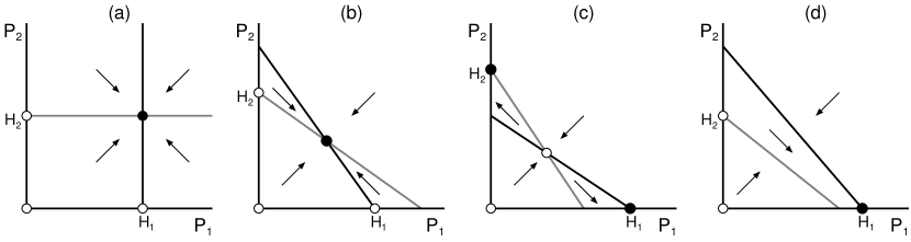
Figure 1: Qualitative configurations of plant isoclines (P1 in black and P2 in gray) when pollinator preferences for plants and densities are fixed. Filled (open) circles represent stable (unstable) equilibria. Circles on the axes correspond to pollinator-dependent carrying capacities $H_{i}$ given by (3).

2.2 Pollinator coexistence

Second, we consider pollinator-only dynamics. For fixed plant densities $P_{i}$ ($i=1,2$), the pollinator sub-system (1c,1d) is the resource competition model of Schoener (1978). Appendix A shows that there are three qualitatively different pollinator equilibria. The equilibrium where both pollinators are extinct $(A_{1},A_{2})=(0,0)$ is unstable if one or both pollinators is viable. Viability conditions for pollinator A1 and A2 are, respectively,

$$a_{1}P_{1}e_{11}u_{1}b_{11}w_{2}+a_{2}P_{2}e_{21}u_{2}b_{21}w_{1} >d_{1}w_{1}w_{2}$$ (5a)

$$a_{1}P_{1}e_{12}v_{1}b_{12}w_{2}+a_{2}P_{2}e_{22}v_{2}b_{22}w_{1} >d_{2}w_{1}w_{2}.$$ (5b)

If neither of the above inequalities holds, both pollinators go extinct. If only one inequality holds then the corresponding pollinator is viable, and for each viable pollinator there is a corresponding single species equilibrium $(A_{1},0)$ or $(0,A_{2}).$ As we see, pollinator viability implies minimum resource requirements (Grover, 1997).

Appendix A shows that there can be at most one pollinator coexistence equilibrium $(\hat{A}_{1},\hat{A}_{2})$. Such an equilibrium is locally asymptotically stable (Appendix A) if

$$(u_{1}b_{11}v_{2}b_{22}-v_{1}b_{12}u_{2}b_{21})(e_{11}u_{1}b_{11}e_{22}v_{2}b_{22}-e_{12}v_{1}b_{12}e_{21}u_{2}b_{21})>0.$$ (6)

The interpretation of condition (6) is similar to that given by León and Tumpson (1975) for two consumers competing for two substitutable resources: “… the competitors coexist if at equilibrium each of them removes at a higher rate that resource which contributes more to its own rate of growth.” To see why this is so, let us assume that plant P1 is better for the growth of A1 ($e_{11}>e_{21}$) and P2 is better for the growth of A2 ($e_{22}>e_{12}$). Then, if pollinator A1 interacts comparatively more strongly with plant P1 than with P2 ($u_{1}b_{11}>u_{2}b_{21}$), and pollinator A2 interacts comparatively more strongly with plant P2 than with P1 ($v_{2}b_{22}>v_{1}b_{12}$), inequality (6) holds.

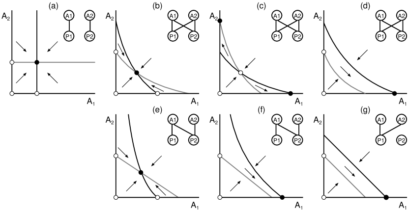
Figure 2: Pollinator isocline configurations (A1 in black and A2 in gray) and qualitative dynamics (arrows), at fixed pollinator preferences. Filled (open) circles represent stable (unstable) equilibria. Isocline shapes depend on interaction topology (inset graphs).

Provided both pollinators are viable (5a and 5b hold), Figure 2 shows all generic pollinator isocline configurations corresponding to different interaction topologies (except symmetries). The top row of this figure is analogous to Figure 1 for plants. Panel (a) shows the case where pollinators specialize on different plants ($u_{1}=1,v_{1}=0$). The A1 isocline is vertical, the A2 isocline is horizontal, and their intersection corresponds to stable pollinator coexistence since pollinators do not compete. Panels (b,c,d) display isoclines for two generalist pollinators (i.e., $0<u_{1}<1$, $0<v_{1}<1$), i.e., both pollinators share both plants. Notice that the isoclines of generalist pollinators are curved and intersect both axes. In (b) an isocline intersection exists and the equilibrium between generalists is globally stable because (6) holds. In (c) an isocline intersection exists but the corresponding equilibrium between generalists is unstable because (6) does not hold and either A1 or A2 wins the competition depending on the initial conditions. In panel (d) the isoclines do not intersect and the pollinator with the highest isocline always wins. In other words condition (6) is irrelevant for coexistence in this case. This outcome happens if e.g., A1 has a much lower mortality and/or higher conversion efficiencies than A2. This case is like the case of competitive dominance between plants (Figure 1d), except that for the plants the isoclines are linear.

Panels (e,f) display isoclines when pollinator A1 is a generalist and A2 is a P2 specialist (i.e., $0<u_{1}<1$, $v_{1}=0$). Like in panels (b,c,d) the isocline of the generalist is curved, but the specialist isocline is linear. Under these condition, condition (6) is trivially satisfied (because $v_{1}=0$). Thus, if both isoclines intersect, the corresponding coexistence equilibrium is always globally stable like in panel (e), and if they do not intersect the species with the highest isocline always wins (e.g., A1 in panel (f)). In other words, competition between a generalist and a specialist pollinator does not admit the bi-stable case (i.e., panel c).

Finally, in panel (g) both pollinators specialize on plant P1, (e.g., $u_{1}=v_{1}=1$). In this case both pollinators have parallel linearly decreasing isoclines, and the pollinator with the higher isocline (i.e., A1 in this case) excludes the other pollinator. This case is like the case of competitive dominance between plants (Figure 1d), except that for the plants the isoclines are not required to be parallel.

3 Population dynamics when pollinator preferences for plants are adaptive

In this section we assume that pollinator preferences adaptively change as plant and pollinator densities change. First (section 3.1), we use a game theoretic approach (Křivan et al., 2008) to derive optimal pollinator preferences at given plant and pollinator densities. Second (section 3.2), we analyze competition between plants at fixed pollinator densities. Third (section 3.3), we analyze competition between pollinators at fixed plant densities.

3.1 Optimal pollinator preferences

Let us consider a mutant pollinator A1 with preference $\tilde{u}_{1}\in[0,1]$ for the first plant and a mutant pollinator A2 with preference $\tilde{v}_{1}\in[0,1]$ in a resident population of pollinators with average preferences $u_{1}$ and $v_{1}$, respectively. The payoff a pollinator obtains when pollinating plant $i$ ($i=1,2$) is given by the per-capita pollinator birth rate. For example, from (1c) the payoff of a pollinator A1 when pollinating plant P2 is $\frac{a_{2}e_{21}b_{21}P_{2}}{w_{2}+u_{2}b_{21}A_{1}+v_{2}b_{22}A_{2}}$. As the resident pollinator distribution between the two plants is the same as are their preferences we see that payoffs depend on the distribution of pollinators between the two plants. Fitnesses of A1 and A2 mutants are defined as their mean payoffs

$$F_{1}(\tilde{u}_{1};u_{1},v_{1}) =\frac{a_{1}e_{11}b_{11}P_{1}}{w_{1}+u_{1}b_{11}A_{1}+v_{1}b_{12}A_{2}}\tilde{u}_{1}+\frac{a_{2}e_{21}b_{21}P_{2}}{w_{2}+u_{2}b_{21}A_{1}+v_{2}b_{22}A_{2}}\tilde{u}_{2},$$ (7a)

$$F_{2}(\tilde{v}_{1};u_{1},v_{1}) =\frac{a_{1}e_{12}b_{12}P_{1}}{w_{1}+u_{1}b_{11}A_{1}+v_{1}b_{12}A_{2}}\tilde{v}_{1}+\frac{a_{2}e_{22}b_{22}P_{2}}{w_{2}+u_{2}b_{21}A_{1}+v_{2}b_{22}A_{2}}\tilde{v}_{2}.$$ (7b)

Throughout the rest of this article we assume that pollinator A1 grows comparatively faster on plant P1 than on P2, and that pollinator A2 grows comparatively faster on plant P2 than on P1, i.e.,

$$(e_{11}b_{11})(e_{22}b_{22})>(e_{21}b_{21})(e_{12}b_{12}).$$ (8)

We want to find pollinator preferences for plants that are evolutionarily stable (Hofbauer and Sigmund, 1998). Interestingly, Appendix B shows that there is no evolutionarily stable preference/strategy where both pollinator species behave as generalists (i.e., preference $(u_{1},v_{1})$ where $0<u_{1}<1$ and $0<v_{1}<1$). In other words, the interaction topology in Figure 2b,c,d does not exist when pollinators preferences are adaptive. In fact either both species are specialists, or one species is a generalist and the other specializes on the plant that makes it grow faster. Table 1 lists all possible ESSs as a function of plant and pollinator population densities. Transitions between ESSs in plant phase space occur along four lines $P_{2}=Q_{i}P_{1}$ $(i=a,b,c,d)$, called isolegs (Rosenzweig, 1981; Pimm and Rosenzweig, 1981; Křivan and Sirot, 2002), where

$$Q_{a}(A_{1},A_{2}) =\frac{a_{1}b_{11}e_{11}(w_{2}+b_{21}A_{1}+b_{22}A_{2})}{a_{2}b_{21}e_{21}w_{1}},$$ (9a)

$$Q_{b}(A_{1},A_{2}) =\frac{a_{1}b_{11}e_{11}(w_{2}+b_{22}A_{2})}{a_{2}b_{21}e_{21}(w_{1}+b_{11}A_{1})},$$ (9b)

$$Q_{c}(A_{1},A_{2}) =\frac{a_{1}b_{12}e_{12}(w_{2}+b_{22}A_{2})}{a_{2}b_{22}e_{22}(w_{1}+b_{11}A_{1})},$$ (9c)

$$Q_{d}(A_{1},A_{2}) =\frac{a_{1}b_{12}e_{12}w_{2}}{a_{2}b_{22}e_{22}(w_{1}+b_{11}A_{1}+b_{12}A_{2})}.$$ (9d)

At fixed pollinator densities isolegs delineate five regions (denoted as I-V in Table 1) in the first quadrant of the $P_{1}P_{2}$ plane where pollinators behave as specialists or generalists. Appendix B shows that when pollinator A1 is a generalist and A2 specializes on P2 (region II in Table 1), the ESS of A1 is

$$u_{1}^{*}=\frac{e_{11}b_{11}a_{1}P_{1}(w_{2}+b_{21}A_{1}+b_{22}A_{2})-e_{21}b_{21}a_{2}P_{2}w_{1}}{b_{11}b_{21}(e_{11}a_{1}P_{1}+e_{21}a_{2}P_{2})A_{1}},$$ (10a)

and when A2 is a generalist and A1 specializes on P1 (region IV in Table 1), the ESS of A2 is

$$v_{1}^{*}=\frac{e_{12}b_{12}a_{1}P_{1}(w_{2}+b_{22}A_{2})-e_{22}b_{22}a_{2}P_{2}(w_{1}+b_{11}A_{1})}{b_{12}b_{22}(e_{12}a_{1}P_{1}+e_{22}a_{2}P_{2})A_{2}}.$$ (10b)

Region	Conditions	ESS $(u_{1},v_{1})$	Description
I	$Q_{a}(A_{1},A_{2})P_{1}<P_{2}$	$(0,0)$	A1 & A2 specialize on P2
II	$Q_{b}(A_{1},A_{2})P_{1}<P_{2}<Q_{a}(A_{1},A_{2})P_{1}$	$(u_{1}^{*},0)$	A1 generalist, A2 specializes on P2
III	$Q_{c}(A_{1},A_{2})P_{1}<P_{2}<Q_{b}(A_{1},A_{2})P_{1}$	$(1,0)$	A1 specializes on P1, A2 specializes on P2
IV	$Q_{d}(A_{1},A_{2})P_{1}<P_{2}<Q_{c}(A_{1},A_{2})P_{1}$	$(1,v_{1}^{*})$	A1 specializes on P1, A2 generalist
V	$P_{2}<Q_{d}(A_{1},A_{2})P_{1}$	$(1,1)$	A1 & A2 specialize on P1

Table 1: Dependence of evolutionarily stable pollinator preferences on plant $(P_{1},P_{2})$ and pollinator densities $(A_{1},A_{2})$. Thresholds $Q_{i}$ $(i=a,b,c,d)$ are given by (9) and $u_{1}^{*}$ and $v_{1}^{*}$ by (10).

In the next section we use isolegs and isoclines to study plant–plant competition.

3.2 Plants compete for pollinator preferences

Here we use isocline analysis to study the dynamics of the plant sub-system at fixed pollinator densities $A_{1}$ and $A_{2}$, when pollinators are adaptive. Unlike in the case with fixed preferences, pollinator isolegs partition the $P_{1}P_{2}$ plane into five regions listed in Table 1. Isolegs $P_{2}=Q_{i}P_{1}$ ($i=a,b,c,d$; see (9)) are rays passing through the origin (dashed lines in Figures 3 and 5). Inequality (8) implies that the slopes of isolegs satisfy $Q_{d}<Q_{c}<Q_{b}<Q_{a}$ and, consequently, regions I, II, III, IV and V are ordered in a clockwise sequence (Figure 3). As a result of this partition of the positive quadrant, plant isoclines are defined piece-wise, and they are considerably more complex when compared to the situation where pollinators have fixed preferences (cf. Figure 3 vs. Figure 1). Plant isoclines in regions I, III, and V are easy to describe analytically (Appendix C). However, in regions II and IV, plant isoclines are highly non-linear and although they can be calculated using some computer algebra software (e.g., Mathematica), the resulting expressions are too complex and they are not useful for further mathematical analysis.

In what follows we will assume that each plant monoculture is viable, i.e., for P1

$$\frac{a_{1}(r_{11}b_{11}A_{1}+r_{12}b_{12}A_{2})}{w_{1}+b_{11}A_{1}+b_{12}A_{2}}>m_{1},$$ (11a)

and for P2

$$\frac{a_{2}(r_{21}b_{21}A_{1}+r_{22}b_{22}A_{2})}{w_{2}+b_{21}A_{1}+b_{22}A_{2}}>m_{2}.$$ (11b)

This means that each plant equilibrates with pollinator densities when alone (section 2.1). Then plant isoclines have the following general properties:

1. Isoclines consist of four connected segments, as shown by e.g., Figure 3a. The isocline of plant P1 (P2) intersects the $P_{1}$ $(P_{2})$ axis at the origin and at its pollinator-dependent carrying capacity in region V (I). These boundary equilibria

   $$(P_{1},P_{2})=\bigg{(}K_{1}\left(1-\frac{m_{1}(w_{1}+b_{11}A_{1}+b_{12}A_{2})}{a_{1}(r_{11}b_{11}A_{1}+r_{12}b_{12}A_{2})}\right),0\bigg{)}$$ (12a)

   and

   $$(P_{1},P_{2})=\bigg{(}0,K_{2}\left(1-\frac{m_{2}(w_{2}+b_{21}A_{1}+b_{22}A_{2})}{a_{2}(r_{12}b_{21}A_{1}+r_{22}b_{22}A_{2})}\right)\bigg{)},$$ (12b)

   are shown as filled circles on the axes of Figures 3 and 5. Appendix C shows that provided these boundary equilibria exist (i.e., they are positive), they are locally asymptotically stable.

2. The isoclines are linear in regions I, III and V, in which both pollinators are specialists. Within these regions, $u_{1}$ and $v_{1}$ remain fixed at 0 or 1. If $c_{2}=0$ $(c_{1}=0)$ the isocline of plant P1 (P2) is vertical (horizontal), as shown in Figure 3 (cf., Figure 1a). If $c_{2}>0$ $(c_{1}>0)$ the isocline of plant P1 (P2) is negatively sloped within these regions, as shown in Figure 5 (cf., Figure 1b,c,d).

3. The isoclines are non-linear in regions II and IV, in which one pollinator is generalist and the other specialist. The segment of the plant P1 (P2) isocline which is in region II (IV) passes through the origin.

4. The isocline of plant P1 (P2) does not cross region I (V). This is because in region I (V), plant P2 (P1) has two pollinators, but P1 (P2) has none and goes extinct in this region.

5. The population density of plant P1 (P2) increases in the region below (to the left) its isocline, and decreases in the region above (to the right).

While there can be at most one interior plant equilibrium when pollinator preferences for plants are fixed (section 2.1), there can be multiple interior equilibria when preferences are adaptive, because isoclines intersect in multiple points.

In the rest of this section we consider two particular scenarios that illustrate the complexities of plant population dynamics under adaptive pollinator preferences:

• Scenario I: Plant population dynamics along the gradient in pollinator A1 density. In this scenario the density of pollinator A2 is kept fixed and both pollinators are equally good for each plant $(r_{11}=r_{12},r_{21}=r_{22})$. Plants do not compete for factors external to pollination $(c_{1}=c_{2}=0)$.

• Scenario II: Plant population dynamics along the gradient in plant inter-specific competition for external factors. In this scenario we assume that plant inter-specific competition is symmetric and we set $c=c_{1}=c_{2}$. We also assume that A1 (A2) is the best pollinator of plant P1 (P2) $(r_{11}>r_{12}$, $r_{22}>r_{21})$.

Both scenarios are parameterized so that plant boundary equilibria (12a) and (12b) exist, i.e., pollinator densities are high enough so that each plant can achieve a positive growth rate when alone.

The main purpose of scenario I is to explore how relative changes in pollinator densities influence plant community composition. An important motivation is the growing interest in the consequences of alien pollinator invasions (Traveset and Richardson, 2006), and the management of pollinator populations (Geslin et al., 2017). To focus solely on plant competition for pollination services, we remove the effect of competition for other factors (by setting competition coefficients equal to zero).

In Scenario II we explore how competition for external factors (e.g., space, nutrients) influences competition between plants for pollinator preferences. Because of condition (8), this scenario also assumes that P1 (P2) and A1 (A2) are better for one another. Such matching can be due to matching in plant and pollinator morphologies (Fontaine et al., 2005).

3.2.1 Scenario I. Effects of changes in pollinator composition: Alternative plant stable states

Figure 3 illustrates plant population dynamics for scenario I. Panel (a) shows the situation where pollinator A1 density is the same as pollinator A2 density. Plant isoclines intersect in region IV, and the vector field indicates that the corresponding equilibrium is unstable. Thus, there is bi-stability: depending on initial conditions either plant P1 or P2 is excluded, and the plant community becomes a monoculture. As density of pollinator A1 increases (panel b), the single plant equilibria (12a) and (12b) increase too. As a result, there are three isocline intersections in regions II, III and IV. The equilibrium in region III is stable (because (4) holds, see Appendix C) and the equilibria in regions II and IV are unstable. Again, plant coexistence depends on initial conditions: if one plant is initially too rare plant population dynamics will converge to a monoculture of the other plant, but if the two plants are initially abundant enough, stable coexistence follows. At the coexistence equilibrium pollinators specialize on different plants (see Table 1). In panel (c) pollinator A1 is more abundant than pollinator A2, and two additional equilibria occur in region II, one stable and the other unstable. Thus, there are two stable coexistence equilibria now (one in region II and the other in region III). At the stable equilibrium that is in region II, pollinator A1 is a generalist and A2 is a plant P2 specialist. As in panel (b), at the equilibrium that lies in region III, pollinators specialize on different plants. Finally, in panel (d), further increase in pollinator A1 leads to a single coexistence equilibrium in region II where A1 is a generalist and A2 plant P2 specialist.

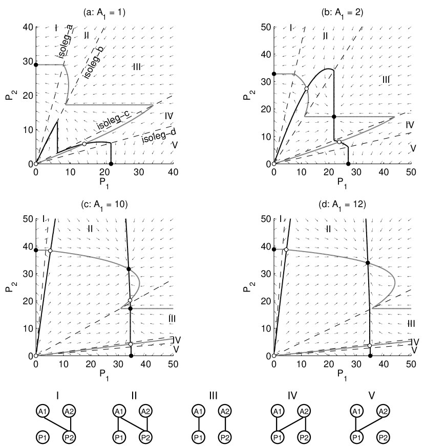
Figure 3: Isoclines of plants P1 (black) and P2 (gray), isolegs (dashed lines), and vector field of plant population dynamics (arrows), under adaptive pollinator preferences and increasing pollinator A1 density ($A_{1}$, scenario I). Filled (open) circles represent stable (unstable) equilibria. Regions of pollinator preference are defined in Table 1, and corresponding interaction topologies are indicated at the bottom. Parameters: $r_{ij}=0.1$, $m_{1}=0.01$, $m_{2}=0.0075$, $c_{i}=0$, $a_{i}=0.4$, $w_{i}=0.25$, $b_{ij}=0.1$, $e_{11}=e_{22}=0.2$, $e_{21}=e_{12}=0.1$, $K_{i}=50$, $A_{2}=1$. Note: parts of the isoclines are not shown in (c,d), but these parts do not intersect at any equilibrium.

Overall, the main effect of increasing pollinator A1 density with respect to A2, is the reduction of region III where both pollinators specialize on different plants, in favor of region II where A1 is a generalist and A2 a specialist. Here we see (Figure 4) that along the gradient in $A_{1}$ density, the topology of the interaction web changes. When population density of A1 is low, both pollinators specialize on different plants. As population density of A1 increases, A1 becomes a generalist. We also observe that plant P2 experiences hysteresis: the stable equilibrium in region III jumps to the stable equilibrium in region II at $A_{1}\approx 11.7$ as pollinator density $A_{1}$ increases, but the stable equilibrium moving along branch II jumps back to the stable equilibrium moving along branch III at $A_{1}\approx 8.7$ when pollinator density $A_{1}$ decreases. Another important consequence of pollinator A1 increase is that region I (V), in which P1 (P2) always decreases, become smaller. This makes easier for plants to invade one another and achieve coexistence.

Figure 4: Bifurcation plot for plant P2 in scenario I. Thin solid lines represent stable equilibria with one plant extinct. Thick solid lines represent stable coexistence equilibria, next to corresponding interaction topology. Dashed lines represent unstable equilibria. Roman numerals (I to V) indicate the location of equilibria within preference regions given by the ESS (Table 1). Labels along the top of the plot correspond to panels in Figure 3.

In summary, scenario I shows that: (i) adaptive foraging preferences can lead to alternative plant coexistence stable states and (ii) continuous changes in pollinator composition (i.e., $A_{1}:A_{2}$ ratio) produce discontinuous changes in plant–pollinator interaction structure.

3.2.2 Scenario II. Effects of plant competition for external factors: Trait-mediated apparent facilitation

Plant dynamics for scenario II are illustrated in Figure 5. The isolegs (dashed lines, (9)) and boundary equilibria (12a) and (12b) do not change across panels (a–d), because they are independent of the competition coefficient $c=c_{1}=c_{2}$. Within regions I, III and V the isoclines are linear while in regions II and IV they are non-linear.

When plant inter-specific competition is low (Figure 5a), plant population dynamics are qualitatively similar to panels (b,d) in Figure 3 of scenario I, i.e., plants can coexist at a stable equilibrium. However, there is an important qualitative difference here: At the coexistence equilibrium both plants attain higher density when compared with their monoculture densities (boundary equilibria). In other words, when inter-specific plant competition is weak, we observe mutual plant facilitation. Let us consider the plant P1 boundary equilibrium in region V. In this region P1 is pollinated by both pollinators. However, when A2 is a poor pollinator for P1 (i.e., $r_{11}>r_{12}$ as assumed in Figure 5), P1 can achieve a higher birth rate when it is pollinated by A1 only. So, if there is an invasion of plant P2 from outside which moves the plant densities in region III, pollinator A1 specializes on plant P1 and plant P2 is pollinated by its best pollinator A2 only. Consequently, the P1 population equilibrium increases above its monoculture level. Appendix C shows that the necessary condition for this facilitation of plant P1 by the presence of P2 to happen is that $r_{11}/r_{12}>1+w_{1}/(b_{11}A_{1})$, which means that pollinator A1 density must be high enough. In addition, such a facilitation can happen only when inter-specific competition between plants is not too high. We remark that this facilitation is not the usual one (Revilla and Křivan, 2016) where an increase in one plant density increases the pollinator density which, in turn, increases the other plant density. This mechanism cannot operate in the current model that assumes pollinator population densities are fixed. The facilitation that we observe here is due to changes in pollinator preferences, where by increasing plant P2 density, pollinator A2 switches from pollinating plant P1 to pollinating P2, which leads to an increase of P1 population density. To distinguish this mechanism from density mediated facilitation caused by increase in pollinator density, we call this mechanism indirect trait-mediated facilitation (sensu Bolker et al., 2003).

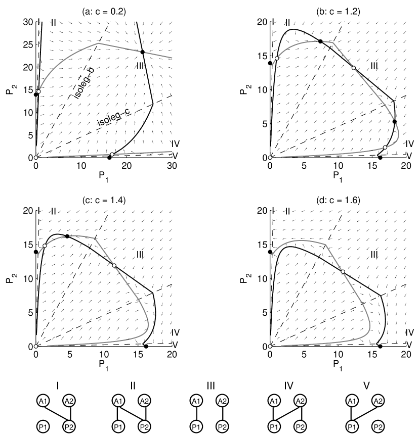
Figure 5: Isoclines of plants P1 (black) and P2 (gray), isolegs (dashed lines), and vector field of plant population dynamics (arrows), under adaptive pollinator preferences and with increasing plant competition ($c_{i}$, scenario II). Filled (open) circles represent stable (unstable) equilibria. Regions of pollinator preference are defined in Table 1, and corresponding interaction topologies are indicated at the bottom. Parameters: $r_{11}=r_{22}=0.5$, $r_{12}=r_{21}=0.1$, $m_{i}=0.02$, $a_{i}=0.1$, $w_{i}=0.1$, $b_{ij}=0.1$, $e_{11}=e_{22}=0.2$, $e_{21}=e_{12}=0.1$, $K_{i}=50$, $A_{1}=11$, $A_{2}=10$. Note: parts of the isoclines are not shown in (a), but these parts do not intersect at any equilibrium.

As inter-specific competition increases, plant equilibrium population densities in region III will be decreasing below those they achieve in a monoculture (boundary equilibria). When plant inter-specific competition is strong so that $c>1$, the equilibrium in region III becomes unstable (i.e., (4) does not hold, see also Appendix C), but plants can still coexist at alternative stable states. In Figure 5b, the local dynamics around the unstable equilibrium in region III is like in Figure 1c, where perturbations cause either plant P1 to displace P2 or vice versa. Like in scenario I, we have two alternative stable states at which both plants coexist. The most abundant plant in each state is the one pollinated by both pollinators. Further increase of the competition coefficient eliminates all equilibria in region IV, but the stable equilibrium in region II remains, with pollinator A1 a generalist and A2 specialized on P2 (Figure 5c). Finally, if competition is too strong there are no equilibria in regions II and IV and we have mutual exclusion (Figure 5d) where, depending on the initial conditions, one plant outcompetes the other plant (cf. Figure 1c).

Figure 6 shows the corresponding bifurcation plot for scenario II. As competition for extrinsic factors (i.e., not for pollination) gets stronger, both plant equilibrium densities tend to decrease, even in the region of alternative stable states $(1\apprle c\apprle 1.3)$ where P1 can be either abundant (stable IV branch) or rare (stable II branch). There is only a small region where plant P1 increases with competition $(0.9\apprle c\apprle 1)$, i.e., where the combined effects of exploitative competition and competition for pollination (i.e., trait-mediated plant facilitation) is more favorable for P1 than for P2 (which decreases, not shown). Notice that in comparison to Figure 4 which shows transitions between two stable interaction topologies, Figure 6 shows transitions between three stable interaction topologies.

Figure 6: Bifurcation plot for plant P1 in scenario II. Lines and labels follow the same conventions of Figure 4. Labels along the top of the plot correspond to panels in Figure 5.

In summary, scenario II shows that: (i) adaptive foraging preferences can result in indirect trait-mediated plant–plant facilitation, by matching plants with their best pollinators; (ii) continuous changes in competition for factors external to pollination can produce discontinuous changes in interaction structure and coexistence for plants competing for pollination services; and (iii) plants can coexist even when inter-specific competition is stronger than intra-specific competition for factors other than pollination. In the next section we use isolegs and isoclines to study pollinator–pollinator competition.

3.3 Pollinators compete for plant resources

In this section we analyze population dynamics of adaptive pollinators at fixed plant densities. Unlike in the case of fixed preferences (Figure 2), now we must partition the first quadrant of the pollinator plane $A_{1}A_{2}$ into different regions using isolegs (Figure 7), according to Table 2 (see Appendix D). The isolegs are linear in $A_{1}$ and they are given by $A_{2}=S_{i}(P_{1},P_{2})A_{1}+I_{i}(P_{1},P_{2})$ (where $i=a,b,c,d$) where slopes and intercepts are

$$\begin{array}[]{lc}S_{a}(P_{1},P_{2})=-\frac{b_{21}}{b_{22}},&I_{a}(P_{1},P_{2})=\frac{a_{2}b_{21}e_{21}P_{2}w_{1}-a_{1}b_{11}e_{11}P_{1}w_{2}}{a_{1}b_{11}b_{22}e_{11}P_{1}},\\[14.22636pt] S_{b}(P_{1},P_{2})=\frac{a_{2}e_{21}b_{21}P_{2}}{a_{1}e_{11}b_{22}P_{1}},&I_{b}(P_{1},P_{2})=\frac{a_{2}b_{21}e_{21}P_{2}w_{1}-a_{1}b_{11}e_{11}P_{1}w_{2}}{a_{1}b_{11}b_{22}e_{11}P_{1}},\\[14.22636pt] S_{c}(P_{1},P_{2})=\frac{a_{2}e_{22}b_{11}P_{2}}{a_{1}e_{12}b_{12}P_{1}},&I_{c}(P_{1},P_{2})=\frac{a_{2}b_{22}e_{22}P_{2}w_{1}-a_{1}b_{12}e_{12}P_{1}w_{2}}{a_{1}b_{12}b_{22}e_{12}P_{1}},\\[14.22636pt] S_{d}(P_{1},P_{2})=-\frac{b_{11}}{b_{12}},&I_{d}(P_{1},P_{2})=\frac{a_{1}b_{12}e_{12}P_{1}w_{2}-a_{2}b_{22}e_{22}P_{2}w_{1}}{a_{2}b_{22}b_{12}e_{22}P_{2}}.\end{array}$$ (13)

Region	Conditions	ESS $(u_{1},v_{1})$	Description
I	$A_{2}<S_{a}A_{1}+I_{a}$	$(0,0)$	A1 & A2 specialize on P2
II	$S_{a}A_{1}+I_{a}<A_{2}<S_{b}A_{1}+I_{b}$	$(u_{1}^{*},0)$	A1 generalist, A2 specializes on P2
III	$S_{b}A_{1}+I_{b}<A_{2}<S_{c}A_{1}+I_{c}$	$(1,0)$	A1 specializes on P1, A2 specializes on P2
IV	$\max\{S_{c}A_{1}+I_{c}\,,\,S_{d}A_{1}+I_{d}\}<A_{2}$	$(1,v_{1}^{*})$	A1 specializes on P1, A2 generalist
V	$A_{2}<S_{d}A_{1}+I_{d}$	$(1,1)$	A1 & A2 specialize on P1

Table 2: ESS as a function of pollinator densities. Isoleg slopes $S_{i}(P_{1},P_{2})$ and intercepts with the $A_{2}$ axis $I_{i}(P_{1},P_{2})$ $(i=a,b,c,d)$ are given by (13), and $u_{1}^{*}$ and $v_{1}^{*}$ by (10).

Compared to isolegs in the plant plane (Figures 3 and 5), in the pollinator plane isolegs neither pass through the origin, nor all have positive slopes. Thus, for given parameter values and plant population densities not all regions from Table 2 exist in the positive quadrant. In general:

1. Regions II, III and IV always occur (see Figure 7). They are separated by the isoleg-b ($A_{2}=S_{b}A_{1}+I_{b}$) and the isoleg-c ($A_{2}=S_{c}A_{1}+I_{c}$) with positive slopes $S_{b}$ and $S_{c}$, respectively. These isolegs do not intersect in the first quadrant of the $A_{1}A_{2}$ plane (Appendix D).

2. Because of (8) the isoleg-c separating IV and III is steeper than the isoleg-b separating III and II $(S_{c}>S_{b})$. Thus, regions II, III and IV are ordered in a counter-clockwise sequence in the positive $A_{1}A_{2}$ plane.

3. Regions I and V are separated from regions II and IV, respectively, by isoleg-a and isoleg-d with negative slopes $S_{a}$ and $S_{d}$. Appendix D shows that at most one of these two regions can exist for given parameters and plant population densities. E.g., in Figure 7a neither of the two regions exist, while in 7b region I exists.

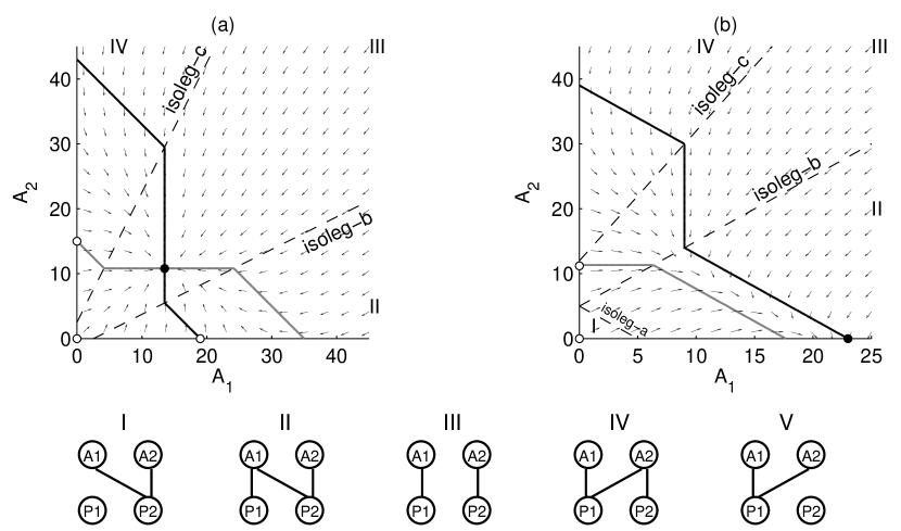
Figure 7: Isoclines of pollinators A1 (black) and A2 (gray), isolegs (dashed lines), and dynamics (vector field), under adaptive pollinator preferences. Filled (open) circles represent stable (unstable) equilibria. Regions of pollinator preference are defined in Table 2, and corresponding interaction topologies are indicated at the bottom. Parameters: $a_{i}=0.4$, $b_{ij}=0.1$, $d_{1}=0.1$, $d_{2}=0.12$, $P_{1}=P_{2}=20$ in all panels; (a) $e_{11}=e_{22}=0.2$, $e_{12}=e_{21}=0.1$, $w_{i}=0.1$; (b) $e_{11}=e_{21}=e_{12}=0.2$, $e_{12}=0.1$, $w_{1}=0.7,w_{2}=0.2$.

The partition of the pollinator plane results in pollinator isoclines that are more complex than in the case of fixed preferences, but considerably simpler than plant isoclines in section 3.2. The isoclines consist of three (e.g., Figure 7a) or two connected segments (e.g., the pollinator A2 isocline in Figure 7b). Regions I and V contain no isocline segments. The segments within regions II and IV are linearly decreasing, and both isoclines are parallel in these two regions (see Appendix D). Thus, generically, pollinators cannot coexist within regions II or IV. This is unlike the case with fixed preferences, where the specialist has a linear isocline and the generalist a curved isocline (Figure 2e,f). Finally, the segments of isoclines in region III are vertical for A1 and horizontal for A2, because pollinators specialize on different plants (like in Figure 2a). Thus, pollinator coexistence can only occur in region III when the vertical segment of A1 and the horizontal segment of A2 intersect, as shown in Figure 7a. Given (8), Appendix D demonstrates that pollinator coexistence by mutual invasion requires

$$\frac{b_{21}e_{21}}{b_{22}e_{22}}<\frac{d_{1}}{d_{2}}<\frac{b_{11}e_{11}}{b_{12}e_{12}},$$ (14)

leading to a stable equilibrium in region III. If $d_{1}/d_{2}$ is too low to meet above inequalities, pollinator A2 goes extinct as shown in Figure 7b, and if $d_{1}/d_{2}$ is too large A1 goes extinct instead. The coexistence scenario in Figure 7a is called the ghost of competition past (Connell, 1980), because competition between pollinators causes selection for different plants which ends competition in the long term. What happens here is that the preference trade-off ( $u_{1}+u_{2}=1$ and $v_{1}+v_{2}=1$) causes disadvantage for the generalist when combining its best and worst resources. This is not the case for the specialist that fully commits to its best resource. Thus, in region II (IV), selection drives A1 (A2) individuals to increase preference towards its preferred plant P1 (P2). As a consequence, pollinators specialize on different plants.

In summary, the results show that population dynamics of two adaptable pollinators competing for two plants do not allow stable coexistence between two generalists, one generalist and one specialist, and two specialists on the same plant. In other words, coexistence demands absolute niche segregation where each pollinator has its own plant.

4 Discussion

In this article we study how pollinator adaptation affects coexistence in a community module consisting of two plants and two pollinators. We assume that pollinators preferences for plants are adaptive and they correspond to evolutionarily stable strategies (ESS) at given plant and pollinator densities. Such strategies cannot be invaded by any other mutants with different strategies. We prove that the strategy where both pollinators are generalists is never evolutionarily stable. Then we study plant–plant and pollinator–pollinator population dynamics. We observe that at fixed pollinator densities, adaptive pollinator preferences for plants lead to complex plant dynamics characterized by alternative stable states. Such alternative states do not exist when interaction strengths between pollinators and plants are fixed. We also observe a trait-mediated facilitation (sensu Bolker et al., 2003) between plants due to changes in pollinator preferences where introduction of an alternative plant can increase population density of the original plant, without increasing pollinator density. When plant densities are fixed, our analysis of pollinator–only dynamics shows that a stable coexistence of a generalist and a specialist pollinator is not possible when both pollinators are adaptive foragers. Thus, at the pollinator coexistence equilibrium, each plant must have its own pollinator.

Our analyses combine an evolutionary approach with population dynamics. The evolutionary approach is based on isolegs (Rosenzweig, 1981; Pimm and Rosenzweig, 1981; Křivan and Sirot, 2002) analysis. Isolegs split the plant (or pollinator) phase space into several regions that are characterized by pollinator specialization or generalism. The population dynamic approach is based on isocline analysis. When compared to standard models of population dynamics, the case where pollinators are adaptive foragers leads to isoclines that are defined piece-wise depending on the pollinator optimal strategy. For example, when interaction strengths between pollinators and plants are fixed (i.e., pollinators are inflexible foragers), plant–plant dynamics follow the Lotka–Volterra competition model with isoclines being straight lines (Figure 1, top row). However, when pollinators are adaptive foragers, plant isoclines are highly non-linear (e.g., Figure 3). It is this emerging non-linearity that shows striking consequences of adaptive pollinator behavior in the interaction web studied in this article.

In order to get insights on plant and pollinator coexistence, we assume that one mutualistic guild, the plants or the pollinators, stays at constant densities, while the other undergoes population dynamics. This is a limitation, but such conditions are not uncommon in nature. E.g., plants can be long lived trees or shrubs, while pollinators can be comparatively short lived, e.g., insects. The assumption of pollinator densities being constant while plants undergo population dynamics can represent situations where plants are short lived (e.g., grasses or forbs), while pollinator densities are mainly controlled by factors other than mutualism (e.g., pollinators may be limited by availability of artificial beehives or tree holes). Another possibility is that plant dynamics take place in a small locality or a patch, and this patch has a certain pollinator carrying capacity which is rapidly filled by visiting pollinators (Feldman et al., 2004) coming from a much larger region. This can be the case of massively introduced managed pollinators, spilling over from mass flowering crops into wild plant communities (Geslin et al., 2017).

4.1 Adaptive pollinator preferences

When two pollinators compete for resources provided by two plants, we predict five qualitatively different pollinator preferences that are evolutionarily stable (Table 1). These strategies are characterized either as full specialization of a pollinator on a single plant or generalism. We proved that the situation where both pollinators are generalists is never evolutionarily stable and it should not be observed in nature. The distribution of pollinator preferences is similar to the ideal free distribution (IFD) of two consumers using two resource patches (Křivan, 2003).

Pollinator preferences were derived under conditions of low species diversity (only four species), and constant population densities. Interestingly, such conditions are approximated in the experiments of Fontaine et al. (2005). These authors used two plant groups: plants with open (P1), and tubular (P2) flowers; and two pollinator groups: syrphid flies (A1), and bumblebees (A2). Each group consisted of three species. This diversity ensures that each pollinator group can use each plant group. However, syrphid flies are morphologically better adapted to open flowers, whereas bumblebees are better adapted to tubular flowers. Plants and pollinators interacted at fixed densities within cages. One experiment found that when alone, each pollinator group displayed generalism. However, when together, syrphids tended to visit open flowers almost exclusively, whereas bumblebees tended to maintain their generalism. This observation corresponds with our partially mixed ESS with one specialist and one generalist pollinator. Further experimentation, with controlled variation of P1:P2 and A1:A2 abundance ratios, will be necessary to test our predictions (Table 1).

4.2 How adaptive preferences change plant coexistence

Analysis of plant dynamics when pollinator densities are fixed indicates that pollinator preferences can modify the plant community to a large extent. Under fixed pollinator preferences, plant population dynamics are described by the Lotka–Volterra competition model. Thus, plants either coexist at an equilibrium, or one plant is outcompeted by the other plant (Figure 1). In the bi-stable case when initial conditions determine the outcome of competition (Figure 1c), the preferred plant that survives has a larger domain of attraction so it is expected to win more frequently. When pollinator preferences are adaptive, initial conditions have major effects on plant coexistence for three main reasons. First, since pollination is obligatory for both plants, coexistence requires that no plant is initially too rare, because otherwise positive feedbacks make the rare plant less preferred and the common plant more preferred (the rich get richer and the poor get poorer situation), causing the rare plant extinction. The same feedbacks prevent invasion of rare plants, unless invaders start above minimum density thresholds. Second, pollinator adaptation enables alternative stable states in plant coexistence. Third, plants can coexist even when their inter-specific competition is so strong that one plant would be outcompeted when pollinators were inflexible foragers.

Many mutualistic models predict critical transitions in community composition as a result of an environmental stress (e.g., warming, habitat fragmentation, changes in phenology). These critical transitions can lead to states of very low diversity, or community collapse when mutualism is obligatory. In large communities, critical transitions are preceded by a gradual accumulation of species extinctions that cause interaction loss (e.g., simulated by random species removal, Jelle Lever et al., 2014). On a much smaller scale (only four species) our scenario I, where the density of pollinator A1 increases while the density of the second pollinator A2 is kept fixed, demonstrates critical transitions (i.e., discontinuous changes both in numbers and the interaction topology) due to interaction loss. In this scenario, transitions between single and alternative stable states in the plant community are due to switches in one pollinator (A1) strategy. When the pollinator is rare it specializes on the best plant (Fig. 3b). As its population increases the pollinator switches to a generalist (Fig. 3c), in response to increased competition. We do not have empirical evidence for transitions like in scenario I, but we can hypothesize one of practical importance. Consider a managed pollinator (e.g., A1 = honeybees) coexisting with wild pollinators (e.g., A2 = bumblebees). We assume that managed pollinators start with high densities e.g., thanks to artificial beehives. Because of competition for plants this large population will generalize (Fontaine et al., 2008), pollinating many plants and maintaining high plant diversity (in Figure 4 this corresponds to pollinator A1 above $A_{1}\approx 8.7$ and plant P2 density given by the solid curve labeled by II). A parasite infestation will cause the managed pollinator population to collapse to much lower densities (Guzmán-Novoa et al., 2010) (below $A_{1}\approx 8.7$ in Figure 4). Competition between pollinators for plants will be lower and they will specialize (pollinator A1 specializes on P1 in Figure 4). This will lead to a critical transition in the plant community where P2 density drops to $P_{2}\approx 17$ (solid line labeled by III). In order to revert back to the condition where P2 had a higher density ($P_{2}\approx 27$ and larger, solid line labeled by II), pollinator A1 must become generalist again, but due to hysteresis the density of this managed pollinator must be raised to levels higher than before the collapse (i.e., A1 must reach population density above $A_{1}\approx 11.7$ in Figure 4), e.g., by providing additional beehives. This hypothetical scenario could be tested using semi-closed experimental plant communities, by controlling the access of massively introduced managed pollinators living nearby (Geslin et al., 2017).

Competition for pollinator preferences can result in plant coexistence at densities that are smaller (scenario I, Figure 3, specially for P2) or larger (scenario II, Figure 5a) than the densities when each plant is alone. The first prediction was widely confirmed empirically (Chittka and Schürkens, 2001; Aizen et al., 2014). Regarding the second prediction, the experiments of Fontaine et al. (2005) discussed before indicate that plant facilitation is a potentially realistic outcome. In that experiment, plants with open flowers (P1) were better adapted to syrphid flies (A1) and vice-versa, whereas plants with tubular flowers (P2) were better adapted to bumblebees (A2). Bumblebees are generalists and they are slightly better at using tubular flowers. When the four groups were placed together, competition forced syrphids to concentrate on open flowers and bumblebees to prefer tubular flowers. At the end of experiment each plant group was taken care of by its best pollinator group, and ended up producing more seeds. This experiment and our predictions demonstrate that given enough functional diversity, i.e., differences in plant and pollinator functional traits, adaptive pollination can improve not only pollinator coexistence but also plant coexistence to the point where plants can end up facilitating one another indirectly. We note that this facilitation between plants can be due to changes in pollinator densities (indirect density-mediated facilitation), or due to changes in trait (indirect trait-mediated facilitation, Bolker et al., 2003) which is caused by changes in pollinator preferences for plants. The interplay between such indirect effects with direct competition between plants for other factors (e.g., space or nutrients, described by competition coefficients), can give rise to alternative stable coexistence states (Figure 5b) (Hernandez, 1998; Gerla and Mooij, 2014; Zhang et al., 2015; Holland and DeAngelis, 2009; Holland et al., 2002).

4.3 How adaptive preferences change pollinator coexistence

The analysis of pollinator population dynamics described by equations (1c,1d) predicts that adaptation of pollinator preferences results in competitive outcomes that are similar to those with fixed preferences: both pollinators can coexist, one always excludes the other, or initial conditions determine which pollinator survives and which goes extinct. In particular, there are no alternative stable states such as we see in the plant sub-system. There are, however, important qualitative differences in the community interaction topology. We already know that the case where both pollinators are generalists is not evolutionarily stable and it cannot occur. However, pollinator population dynamics also exclude pollinator stable coexistence in the case where one pollinator is a specialist and the other a generalist. Thus, when pollinators adapt their foraging preferences with changing population numbers, only pollinators that specialize on different plants can coexist (Figure 7a). As a result, both pollinators stop to compete (the ghost of competition past, Connell, 1980).

We get similar conclusions from numerical simulations of the full four species system (1) with adaptive pollinator preferences (Table 1 or 2): pollinators either specialize on different plants, or specialist pollinators are excluded by generalists (Appendix E shows representative simulations). These results suggest that plant coexistence at alternative states is unlikely when both plant and pollinator dynamics operate on similar time scales.

These conclusions have important implications for systems containing many pollinator species. Most real plant–pollinator interaction networks are nested (Bascompte and Jordano, 2007). This means that a minority of generalist pollinators can interact with many plants, but a majority of more specialized pollinators interact with a few plants only, typically subsets of the plants used by the generalists. This causes a disadvantage for specialized pollinators that have to compete for resources with generalist competitors. Numerical simulations show that adaptive foraging tends to reduce the effect of nestedness on pollinator diet overlap (Valdovinos et al., 2016). As a consequence, specialist pollinators experience less competition, pollination for plants with less pollinators becomes more efficient, and more plants and pollinators can coexist in the long term. We observe the same mechanism in our two-pollinator–two-plant interaction module. For example, consider a generalist pollinator A1 and a specialist A2 (i.e., $0<u_{1}<1,v_{1}=0$) as a caricature of a nested network. Such interaction topology can be dynamically stable when preferences of generalist pollinators are fixed (Figure 2e), but not when preferences adapt in which case either (i) both pollinators specialize on different plants (Figure 7a) or (ii) the specialist goes extinct (Figure 7b). In the first case nestedness is eliminated as the pollinator A1 becomes a specialist.

4.4 Conclusions

As the take-home-message, our analysis of a two-plant–two-pollinator interaction web demonstrates that adaptation of pollinator preferences for plants causes important changes in the structure and dynamics of plant and pollinator communities. First, when pollinator preferences are fixed, interactions between plants follow the Lotka–Volterra competitive dynamics when pollinator densities are held constant. When plant densities are fixed, coexistence of generalist pollinators is possible. Second, when pollinator preferences adapt in order to maximize fitness, plant competitive dynamics become more complex and plant coexistence at alternative stable states and indirect plant–plant facilitation is possible, if pollinator densities are held constant. At fixed plant densities competition between adaptive pollinators requires pollinators specialize on different plants.

Appendix A Coexistence conditions for pollinators with fixed preferences

We set $\alpha_{ij}=a_{i}P_{i}e_{ij}$ and $\beta_{i1}=u_{i}b_{i1},$ $\beta_{i2}=v_{i}b_{i2}$ and re-write the pollinator sub-system (1c, 1d) as

$$\frac{dA_{1}}{dt} =\left\{\frac{\alpha_{11}\beta_{11}}{w_{1}+\beta_{11}A_{1}+\beta_{12}A_{2}}+\frac{\alpha_{21}\beta_{21}}{w_{2}+\beta_{21}A_{1}+\beta_{22}A_{2}}-d_{1}\right\}A_{1}$$

$$\frac{dA_{2}}{dt} =\left\{\frac{\alpha_{12}\beta_{12}}{w_{1}+\beta_{11}A_{1}+\beta_{12}A_{2}}+\frac{\alpha_{22}\beta_{22}}{w_{2}+\beta_{21}A_{1}+\beta_{22}A_{2}}-d_{2}\right\}A_{2}.$$ (A.1)

Model (A.1) has the trivial equilibrium $(A_{1},A_{2})=(0,0).$ When $A_{2}=0$, the per-capita population growth rate $dA_{1}/(A_{1}dt)$ of pollinator A1 decreases monotonically with $A_{1}$. Provided the per capita birth rate of pollinator 1 when $A_{1}=A_{2}=0$ is larger than is its per capita population death rate, i.e.,

$$\alpha_{11}\beta_{11}w_{2}+\alpha_{21}\beta_{21}w_{1}>d_{1}w_{1}w_{2}$$ (A.2)

there is exactly one A1-only equilibrium

$$(A_{1},0)=\bigg{(}\frac{-b+\sqrt{b^{2}-4ac}}{2a},0\bigg{)},$$

where $a=d_{1}\beta_{11}\beta_{21}$, $b=d_{1}(w_{2}\beta_{11}+w_{1}\beta_{21})-(\alpha_{11}+\alpha_{21})\beta_{11}\beta_{21}$ and $c=d_{1}w_{1}w_{2}-w_{2}\alpha_{11}\beta_{11}-w_{1}\alpha_{21}\beta_{21}$.

If the opposite inequality in (A.2) holds, the per-capita population growth rate of pollinator 1 is always negative and the pollinator goes extinct. By symmetry, if

$$\alpha_{12}\beta_{12}w_{2}+\alpha_{22}\beta_{22}w_{1}>d_{2}w_{1}w_{2}$$ (A.3)

there is a unique A2-only equilibrium.

Provided $\beta_{11}\beta_{22}-\beta_{12}\beta_{21}\neq 0$, $d_{2}\alpha_{11}\beta_{11}-d_{1}\alpha_{12}\beta_{12}\neq 0$, and $d_{2}\alpha_{21}\beta_{21}-d_{1}\alpha_{22}\beta_{22}\neq 0,$ model (A.1) has at most one coexistence equilibrium

$$\hat{A}_{1} =\frac{w_{2}\beta_{12}-w_{1}\beta_{22}+\frac{(\alpha_{11}\alpha_{22}\beta_{11}\beta_{22}-\alpha_{12}\alpha_{21}\beta_{12}\beta_{21})[d_{1}(\alpha_{12}+\alpha_{22})\beta_{12}\beta_{22}-d_{2}(\alpha_{21}\beta_{12}\beta_{21}+\alpha_{11}\beta_{11}\beta_{22})]}{(d_{2}\alpha_{11}\beta_{11}-d_{1}\alpha_{12}\beta_{12})(d_{2}\alpha_{21}\beta_{21}-d_{1}\alpha_{22}\beta_{22})}}{\beta_{11}\beta_{22}-\beta_{12}\beta_{21}}$$

$$\hat{A}_{2} =\frac{w_{1}\beta_{21}-w_{2}\beta_{11}+\frac{(\alpha_{11}\alpha_{22}\beta_{11}\beta_{22}-\alpha_{12}\alpha_{21}\beta_{12}\beta_{21})[d_{2}(\alpha_{11}+\alpha_{21})\beta_{11}\beta_{21}-d_{1}(\alpha_{12}\beta_{12}\beta_{21}+\alpha_{22}\beta_{11}\beta_{22})]}{(d_{2}\alpha_{11}\beta_{11}-d_{1}\alpha_{12}\beta_{12})(d_{2}\alpha_{21}\beta_{21}-d_{1}\alpha_{22}\beta_{22})}}{\beta_{11}\beta_{22}-\beta_{12}\beta_{21}}$$ (A.4)

if $\hat{A}_{1}>0$ and $\hat{A}_{2}>0.$

Now we study the local asymptotic stability of the equilibria. The jacobian of (A.1) is

$$\mathbf{J}=\left[\begin{array}[]{cc}G_{1}-A_{1}\left(\frac{\alpha_{11}\beta_{11}^{2}}{W_{1}^{2}}+\frac{\alpha_{21}\beta_{21}^{2}}{W_{2}^{2}}\right)&-A_{1}\left(\frac{\alpha_{11}\beta_{11}\beta_{12}}{W_{1}^{2}}+\frac{\alpha_{21}\beta_{21}\beta_{22}}{W_{2}^{2}}\right)\\ -A_{2}\left(\frac{\alpha_{12}\beta_{11}\beta_{12}}{W_{1}^{2}}+\frac{\alpha_{22}\beta_{21}\beta_{22}}{W_{2}^{2}}\right)&G_{2}-A_{2}\left(\frac{\alpha_{12}\beta_{12}^{2}}{W_{1}^{2}}+\frac{\alpha_{22}\beta_{22}^{2}}{W_{2}^{2}}\right)\end{array}\right]$$ (A.5)

where

$$G_{1}(A_{1},A_{2}) =\frac{\alpha_{11}\beta_{11}}{w_{1}+\beta_{11}A_{1}+\beta_{12}A_{2}}+\frac{\alpha_{21}\beta_{21}}{w_{2}+\beta_{21}A_{1}+\beta_{22}A_{2}}-d_{1}$$ (A.6)

$$G_{2}(A_{1},A_{2}) =\frac{\alpha_{12}\beta_{12}}{w_{1}+\beta_{11}A_{1}+\beta_{12}A_{2}}+\frac{\alpha_{22}\beta_{22}}{w_{2}+\beta_{21}A_{1}+\beta_{22}A_{2}}-d_{2}$$ (A.7)

and

$$W_{1}(A_{1},A_{2}) =w_{1}+\beta_{11}A_{1}+\beta_{12}A_{2}$$ (A.8)

$$W_{2}(A_{1},A_{2}) =w_{2}+\beta_{21}A_{1}+\beta_{22}A_{2}.$$ (A.9)

At the trivial equilibrium the jacobian is diagonal and its eigenvalues are $\lambda_{1}=G_{1}(0,0)$ and $\lambda_{2}=G_{2}(0,0)$. Thus, the trivial equilibrium is unstable if any of (A.2) or (A.3) hold. At the A1-only equilibrium $G_{1}(A_{1},0)=0$ and the eigenvalues are

$$\lambda_{1}=-A_{1}\left(\frac{\alpha_{11}\beta_{11}^{2}}{W_{1}^{2}}+\frac{\alpha_{21}\beta_{21}^{2}}{W_{2}^{2}}\right)\,,\,\lambda_{2}=G_{2}(A_{1},0).$$

Thus, stability depends on the sign of $G_{2}(A_{1},0)$. If $G_{2}(A_{1},0)<0$ pollinator 1 is stable against invasion by pollinator 2, if $G_{2}(A_{1},0)>0$ pollinator 1 can be invaded by pollinator 2. $G_{2}(A_{1},0)$ can be evaluated explicitly, but the resulting expression is quite complex and we do not give it here. By symmetry, the A2-only equilibrium is stable against invasion by pollinator 1 if $G_{1}(0,A_{2})<0$ and unstable if $G_{1}(0,A_{2})>0$.

Provided that the coexistence equilibrium exists (i.e., $\hat{A}_{1}>0,\hat{A}_{2}>0$ in A.4), then $G_{1}(\hat{A}_{1},\hat{A}_{2})=G_{2}(\hat{A}_{1},\hat{A}_{2})=0$ by definition. Thus the trace of the jacobian is negative, which means that stability depends on the sign of the jacobian determinant, which is

$$\Delta=\frac{\hat{A}_{1}\hat{A}_{2}}{(W_{1}W_{2})^{2}}(\beta_{11}\beta_{22}-\beta_{12}\beta_{21})(\alpha_{11}\alpha_{22}\beta_{11}\beta_{22}-\alpha_{12}\alpha_{21}\beta_{12}\beta_{21}).$$ (A.10)

If $\Delta>0$ the equilibrium is locally stable, if $\Delta<0$ it is unstable. If we replace back the definitions of $\alpha$’s and $\beta$’s in (A.10) the stability condition reads

$$(u_{1}b_{11}v_{2}b_{22}-v_{1}b_{12}u_{2}b_{21})(e_{11}e_{22}u_{1}b_{11}v_{2}b_{22}-e_{12}e_{21}v_{1}b_{12}u_{2}b_{21})>0.$$

The above results can be used to study coexistence of specialized pollinators. First, we consider specialized pollinators pollinating a single plant. For example, let us assume that both pollinators pollinate plant P1 only, i.e., $u_{1}=v_{1}=1$. Then $\beta_{11}=\beta_{12}=0$ and substituting these values in (A.1) shows that the two isoclines are parallel lines, i.e., generically, there is no equilibrium. The same conclusion holds in the case where both pollinators specialize on plant P2. Thus, two specialist pollinators cannot survive on a single plant.

Second, we consider two pollinators that specialize on different plants (either $\beta_{12}=\beta_{21}=0$ or $\beta_{11}=\beta_{22}=0$). For example, when $\beta_{12}=\beta_{21}=0$ the interior equilibrium (A.4) is

$$(\hat{A}_{1},\hat{A}_{2})=\left(\frac{\alpha_{11}}{d_{1}}-\frac{w_{1}}{\beta_{11}},\frac{\alpha_{22}}{d_{2}}-\frac{w_{2}}{\beta_{22}}\right)$$

and stability condition (A.10) holds. The case where $\beta_{11}=\beta_{22}=0$ is similar.

Appendix B ESS and Nash equilibria

Throughout this appendix we assume that inequality (8) holds. From (7a) and (7b), for a given pollinator distribution $(u_{1},v_{1})\in[0,1]\times[0,1]$, pollinator A1 payoffs when pollinating exclusively plant P1 or plant P2 are

$$V_{1}(u_{1},v_{1})=\frac{a_{1}e_{11}b_{11}P_{1}}{w_{1}+u_{1}b_{11}A_{1}+v_{1}b_{12}A_{2}},\;\;\;V_{2}(u_{1},v_{1})=\frac{a_{2}e_{21}b_{21}P_{2}}{w_{2}+(1-u_{1})b_{21}A_{1}+(1-v_{1})b_{22}A_{2}}.$$

Similarly, pollinator 2 payoffs are

$$W_{1}(u_{1},v_{1})=\frac{a_{1}e_{12}b_{12}P_{1}}{w_{1}+u_{1}b_{11}A_{1}+v_{1}b_{12}A_{2}},\;\;\;W_{2}(u_{1},v_{1})=\frac{a_{2}e_{22}b_{22}P_{2}}{w_{2}+(1-u_{1})b_{21}A_{1}+(1-v_{1})b_{22}A_{2}}.$$

First, we consider ESS at which both pollinators are specialists. We start with the case where both pollinators specialize on plant 1. Strategy $(u_{1},v_{1})=(1,1)$ is an ESS provided $V_{1}(1,1)>V_{2}(1,1)$ and $W_{1}(1,1)>W_{2}(1,1)$. These inequalities are equivalent to $P_{2}<\frac{a_{1}b_{11}e_{11}w_{2}}{a_{2}b_{21}e_{21}(w_{1}+b_{11}A_{1}+b_{12}A_{2})}P_{1}$ and $P_{2}<Q_{d}P_{1}$, where $Q_{d}$ is given in (9d). Inequality (8) implies that $Q_{d}<\frac{a_{1}b_{11}e_{11}w_{2}}{a_{2}b_{21}e_{21}(w_{1}+b_{11}A_{1}+b_{12}A_{2})}$. Consequently, for $P_{2}<Q_{d}P_{1}$ strategy $(u_{1},v_{1})=(1,1)$ is the ESS. Now we consider the case where pollinator 1 specializes on plant 1 and pollinator 2 on plant 2. Strategy $(u_{1},v_{1})=(1,0)$ is an ESS provided $V_{1}(1,0)>V_{2}(1,0)$ and $W_{2}(1,0)>W_{1}(1,0)$. These inequalities are equivalent to $Q_{b}P_{1}>P_{2}>Q_{c}P_{1}$ where $Q_{b}$ is given in (9b). Now we consider the case where both pollinators specialize on plant 2. Strategy $(u_{1},v_{1})=(0,0)$ is an ESS provided $V_{2}(0,0)>V_{1}(0,0)$ and $W_{2}(0,0)>W_{1}(0,0)$. These inequalities are equivalent to $P_{2}>Q_{a}P_{1}$ where $Q_{a}$ is given in (9d) and $P_{2}>\frac{a_{1}b_{12}e_{12}(w_{2}+b_{21}A_{1}+b_{22}A_{2})}{a_{2}b_{22}e_{22}w_{1}}P_{1}$. Inequality (8) implies that $Q_{a}>\frac{a_{1}b_{12}e_{12}(w_{2}+b_{21}A_{1}+b_{22}A_{2})}{a_{2}b_{22}e_{22}P_{2}w_{1}}$. Consequently, for $P_{2}>Q_{a}P_{1}$ strategy $(u_{1},v_{1})=(0,0)$ is the ESS. Now we consider the case where pollinator 1 specializes on plant 2 and pollinator 2 on plant 1. Strategy $(u_{1},v_{1})=(0,1)$ is an ESS provided $V_{2}(0,1)>V_{1}(0,1)$ and $W_{1}(0,1)>W_{2}(0,1)$. These inequalities are equivalent to $P_{2}>Q_{b}P_{1}$ and $P_{2}<Q_{c}P_{1}.$ Inequality (8) implies that $Q_{b}>Q_{c}$. Consequently, $(u_{1},v_{1})=(0,1)$ is never an ESS.

Second, we consider ESSs when the first pollinator is a generalist while the second pollinator is a specialist. Let us assume that the second pollinator specializes on plant 2, i.e., we seek ESS in the form $(u_{1},0)$ where $0<u_{1}<1$. Such a strategy must satisfy $V_{1}(u_{1},0)=V_{2}(u_{1},0)$ and $W_{2}(u_{1},0)>W_{1}(u_{1},0)$. Equality $V_{1}(u_{1},0)=V_{2}(u_{1},0)$ leads to

$$u_{1}^{*}=\frac{a_{1}b_{11}e_{11}P_{1}(w_{2}+b_{21}A_{1}+b_{22}A_{2})-a_{2}b_{21}e_{21}P_{2}w_{1}}{A_{1}b_{11}b_{21}(a_{1}e_{11}P_{1}+a_{2}e_{21}P_{2})}.$$

This value is between 0 and 1 provided $Q_{b}P_{1}<P_{2}<Q_{q}P_{1}$. Inequality (8) implies that $W_{2}(u_{1}^{*},0)>W_{1}(u_{1}^{*},0)$. Thus, $(u_{1}^{*},0)$ is a Nash equilibrium. To prove it is also an ESS, we need to verify its stability. Because functions $V_{i}$ ($i=1,2$) are non-linear in $u_{1}$, we use the local ESS condition (Hofbauer and Sigmund, 1998) $u_{1}^{*}V_{1}(u_{1},0)+u_{2}^{*}V_{2}(u_{1},0)>u_{1}V_{1}(u_{1},0)+u_{2}V_{2}(u_{1},0)$ for every $(u_{1},u_{2})$ ($u_{1}+u_{2}=1$, $u_{1}>0$, $u_{2}>1$) close to (but different from) $(u_{1}^{*},u_{2}^{*}).$ This condition is equivalent to

$$\frac{(a_{2}b_{11}e_{11}P_{1}(A_{2}b_{22}+A_{1}(b_{21}-b_{21}u_{1})+w_{2}))^{2}}{A_{1}b_{11}b_{21}(a_{1}e_{11}P_{1}+a_{2}e_{21}P_{2})(A_{1}b_{11}u_{1}+w_{1})(A_{2}b_{22}+A_{1}(b_{21}-b_{21}u_{1})+w_{2})}>0.$$ (A.11)

The numerator is positive and the denominator equals to 0 for $u_{1}=-\frac{w_{1}}{A_{1}b_{11}}<0$ and $u_{1}=\frac{A_{1}b_{21}+A_{2}b_{22}+w_{2}}{A_{1}b_{21}}>1.$ Because the denominator is a quadratic function and its graph is an upside down parabola, inequality (A.11) holds for all $0<u_{1}<1$. This shows that $(u_{1},v_{1})=(u_{1}^{*},0)$ is an ESS.

Now we assume that the second pollinator specializes on plant 1, i.e., we seek ESS in the form $(u_{1},1)$ where $0<u_{1}<1$. Such a strategy must satisfy $V_{1}(u_{1},1)=V_{2}(u_{1},1)$ and $W_{1}(u_{1},1)>W_{2}(u_{1},1)$. The equality leads to

$$u_{1}^{*}=\frac{a_{1}b_{11}e_{11}P_{1}(w_{2}+b_{21}A_{1})-a_{2}b_{21}e_{21}P_{2}(w_{1}+b_{12}A_{2})}{A_{1}b_{11}b_{21}(a_{1}e_{11}P_{1}+a_{2}e_{21}P_{2})}.$$

Then

$$W_{1}(u_{1}^{*},1) =\frac{b_{12}b_{21}e_{12}(a_{1}e_{11}P_{1}+a_{2}e_{21}P_{2})}{b_{21}e_{11}(A_{1}b_{11}+A_{2}b_{12}+w_{1})+b_{11}e_{11}w_{2}}$$

$$W_{2}(u_{1}^{*},1) =\frac{b_{11}b_{22}e_{22}(a_{1}e_{11}P+a_{2}e_{21}P_{2})}{b_{21}e_{21}(A_{1}b_{11}+A_{2}b_{12}+w_{1})+b_{11}e_{21}w_{2}}$$

and inequality (8) implies that $W_{2}(u_{1}^{*},1)>W_{1}(u_{1}^{*},1)$ and thus $(u_{1}^{*},1)$ is never an ESS.

Third, we consider ESSs when the first pollinator is a specialist while the second pollinator is a generalist. Let us assume that the first pollinator specializes on plant P1, i.e., we seek ESS in the form $(1,v_{1})$ where $0<v_{1}<1$. Such a strategy must satisfy $V_{1}(1,v_{1})>V_{2}(1,v_{1})$ and $W_{1}(1,v_{1})=W_{2}(1,v_{1})$. The equality leads to

$$v_{1}^{*}=\frac{a_{1}b_{12}e_{12}P_{1}(w_{2}+b_{22}A_{2})-a_{2}b_{22}e_{22}P_{2}(w_{1}+b_{11}A_{1})}{A_{2}b_{12}b_{22}(a_{1}e_{12}P_{1}+a_{2}e_{22}P_{2})}.$$

This value is between 0 and 1 provided $Q_{d}P_{1}<P_{2}<Q_{c}P_{1}$. Inequality (8) implies that $V_{1}(1,v_{1}^{*})>V_{2}(1,v_{1}^{*})$. The local ESS condition requires $v_{1}^{*}W_{1}(1,v_{1})+v_{2}^{*}W_{2}(1,v_{1})>v_{1}W_{1}(1,v_{1})+v_{2}W_{2}(1,v_{1})$ for every $(v_{1},v_{2})$ ($v_{1}+v_{2}=1$, $v_{1}>0$, $v_{2}>1$) close to (but different from) $(v_{1}^{*},v_{2}^{*}).$ This condition is equivalent to

$$\frac{(a_{1}b_{12}e_{12}P_{1}(A_{2}b_{22}(v_{1}-1)-w_{2})+a_{2}b_{22}e_{22}P_{2}(A_{1}b_{11}+A_{2}b_{12}v_{1}+w_{1}))^{2}}{A_{2}b_{12}b_{22}(w_{2}-A_{2}b_{22}(v_{1}-1))(a_{1}e_{12}P_{1}+a_{2}e_{22}P_{2})(A_{1}b_{11}+A_{2}b_{12}v_{1}+w_{1})}>0.$$ (A.12)

The numerator is positive and the denominator equals to 0 for $v_{1}=-\frac{A_{1}b_{11}+w_{1}}{A_{2}b_{12}}<0$ and $v_{1}=\frac{w_{2}}{A_{2}b_{22}}+1>1.$ Because the denominator is a quadratic function and its graph is an upside down parabola, inequality (A.12) holds for all $0<v_{1}<1$. This shows that $(u_{1},v_{1})=(1,v_{1}^{*})$ is an ESS.

Now we assume that the first pollinator specializes on plant P2, i.e., we seek ESS in the form $(0,v_{1})$ where $0<v_{1}<1$. Such a strategy must satisfy $V_{2}(0,v_{1})>V_{1}(0,v_{1})$ and $W_{1}(0,v_{1})=W_{2}(0,v_{1})$. The equality leads to

$$v_{1}^{*}=\frac{a_{1}b_{12}e_{12}P_{1}(w_{2}+b_{21}A_{1}+b_{22}A_{2})-a_{2}b_{22}e_{22}P_{2}w_{1}}{A_{2}b_{12}b_{22}(a_{1}e_{12}P_{1}+a_{2}e_{22}P_{2})}.$$

However, inequality (8) implies that $V_{1}(0,v_{1}^{*})>V_{2}(0,v_{1}^{*})$ so that no ESS in the form $(0,v_{1})$ exists.

Fourth, we consider the case where both pollinators are generalists. This situation corresponds to ESS of the form $(u_{1},v_{1})$ with $0<u_{1}<1$ and $0<v_{1}<1$. Such an ESS must satisfy $V_{1}(u_{1},v_{1})=V_{2}(u_{1},v_{1})$ and $W_{1}(u_{1},v_{1})=W_{2}(u_{1},v_{1})$. These equalities are equivalent to

$$\begin{array}[]{lll}a_{1}e_{11}b_{11}P_{1}(w_{2}+u_{2}b_{21}A_{1}+v_{2}b_{22}A_{2})&=&a_{2}e_{21}b_{21}P_{2}(w_{1}+u_{1}b_{11}A_{1}+v_{1}b_{12}A_{2})\\[5.69046pt] a_{1}e_{12}b_{12}P_{1}(w_{2}+u_{2}b_{21}A_{1}+v_{2}b_{22}A_{2})&=&a_{2}e_{22}b_{22}P_{2}(w_{1}+u_{1}b_{11}A1+v_{1}b_{12}A_{2}).\end{array}$$

Because $w_{1}+u_{1}b_{11}A_{1}+v_{1}b_{12}A_{2}>0$ and $w_{2}+u_{2}b_{21}A_{1}+v_{2}b_{22}A_{2}>0$, inequality (8) implies that these two equations do not have any solution $(u_{1},v_{1})\in[0,1]\times[0,1]$. Thus, it is impossible for both pollinators to be generalists.

Appendix C Plant dynamics in regions I, III and V

First we calculate plant P1 boundary equilibrium. From Table 1 it follows that this equilibrium is in region V where both pollinators pollinate P1. Substituting $(u_{1},v_{1})=(1,1)$ in (1a) and (1b), and solving for equilibria when $P_{1}\neq 0$ and $P_{2}=0$ leads to equilibrium (12a).

The plant population dynamics in region V are

$$\frac{dP_{1}}{dt} =\left(\frac{a_{1}(r_{11}b_{11}A_{1}+r_{12}b_{12}A_{2})}{w_{1}+b_{11}A_{1}+b_{12}A_{2}}\left(1-\frac{P_{1}+c_{2}P_{2}}{K_{1}}\right)-m_{1}\right)P_{1}$$

$$\frac{dP_{2}}{dt} =-m_{2}P_{2},$$

and provided plant 1 is viable (i.e., (11a) holds), equilibrium (12a) exists (is positive) and is locally asymptotically stable. Following the same steps above mutatis mutandis, leads to equation (12b) for plant P2 boundary equilibrium in region I (where ESS is $(u_{1},v_{1})=(0,0)$, see Table 1). Analogously, if (11b) holds then (12b) exists and is locally asymptotically stable.

Now we consider plant population dynamics in region III. According to Table 1 the ESS strategy in this region is $(u_{1},v_{1})=(1,0)$, i.e., pollinator A1 (A2) interacts only with plant P1 (P2). Substituting these preferences in (1a) and (1b), plant population dynamics in region III are described by the Lotka–Volterra competition model

$$\frac{dP_{1}}{dt} =(s_{1}-m_{1})P_{1}\left(1-\frac{P_{1}+c_{2}P_{2}}{H_{1}}\right)$$

$$\frac{dP_{2}}{dt} =(s_{2}-m_{2})P_{2}\left(1-\frac{P_{2}+c_{1}P_{1}}{H_{2}}\right),$$

where

$$s_{1} =\frac{a_{1}r_{11}b_{11}A_{1}}{w_{1}+b_{11}A_{1}},\;\;s_{2}=\frac{a_{2}r_{22}b_{22}A_{2}}{w_{2}+b_{22}A_{2}},\;\;H_{1}=K_{1}\left(1-\frac{m_{1}}{s_{1}}\right),\;\;H_{2}=K_{2}\left(1-\frac{m_{2}}{s_{2}}\right).$$

Plant population dynamics in region III depend on the position of plant isoclines

$$P_{1}+c_{2}P_{2} =H_{1}$$

$$P_{2}+c_{1}P_{1} =H_{2}.$$

Provided the plant isoclines intersect in region III, the coexistence equilibrium is

$$(\hat{P}_{1},\hat{P}_{2})=\left(\frac{H_{1}-c_{2}H_{2}}{1-c_{1}c_{2}},\frac{H_{2}-c_{1}H_{1}}{1-c_{1}c_{2}}\right).$$ (A.13)

For (A.13) to be in region III, it must satisfy $Q_{b}\hat{P}_{1}<\hat{P}_{2}<Q_{c}\hat{P}_{1}$, where $Q_{b}$ and $Q_{c}$ are given in (9b) and (9c), respectively. Substituting $Q_{b}$ , $Q_{c}$ and (A.13) we get

$$\frac{b_{21}e_{21}}{b_{11}e_{11}}<\frac{a_{1}(w_{2}+b_{22}A_{2})(H_{1}-c_{2}H_{2})}{a_{2}(w_{1}+b_{11}A_{1})(H_{2}-c_{1}H_{1})}<\frac{b_{22}e_{22}}{b_{12}e_{12}}.$$ (A.14)

Provided (A.14) holds, the local stability of (A.13) depends on the competition coefficients. From the Lotka–Volterra theory (A.13) is locally stable if $c_{1}c_{2}<1$. If $c_{1}c_{2}>1$, (A.13) is unstable, and trajectories will approach either isoleg-b and cross into region II, or approach isoleg-c and cross into region IV depending on the initial conditions. If (A.14) does not hold there is no plant equilibrium in region III.

In the special case where $c_{1}=c_{2}=0$, the stable equilibrium in region III is

$$(\hat{P}_{1},\hat{P}_{2})=(H_{1},H_{2})=\bigg{(}\frac{K_{1}(A_{1}b_{11}(a_{1}r_{11}-m_{1})-m_{1}w_{1})}{a_{1}A_{1}b_{11}r_{11}},\frac{K_{2}(A_{2}b_{22}(a_{2}r_{22}-m_{2})-m_{2}w_{2})}{a_{2}A_{2}b_{22}r_{22}}\bigg{)}.$$

At this equilibrium plant 1 density is higher than is the plant density at the boundary equilibrium (12a) in region V iff

$$\frac{r_{11}}{r_{12}}>1+\frac{w_{1}}{b_{11}A_{1}}.$$

This shows that provided $r_{11}>r_{12}$ and pollinator A1 is abundant enough, plant P1 density at the interior equilibrium in region III will be higher than is the plant P1 density at the boundary equilibrium. Analogous conclusions apply to plant P2.

Appendix D Coexistence conditions for pollinators with adaptive preferences

Using Table 1 in the main text, we rewrite isolegs characterizing regions I-V in terms of pollinator densities. For example, isoleg-a that separates regions I and II in the plant plane $P_{1}P_{2}$ is given by equation $\frac{P_{2}}{P_{1}}=Q_{a}(A_{1},A_{2})=\frac{a_{1}b_{11}e_{11}(w_{2}+b_{21}A_{1}+b_{22}A_{2})}{a_{2}b_{21}e_{21}w_{1}}.$ Solving for $A_{2}$ leads to isoleg-a in the pollinator plane

$$A_{2}=S_{a}A_{1}+I_{a}=-\frac{b_{21}}{b_{22}}A_{1}+\frac{a_{2}b_{21}e_{21}P_{2}w_{1}-a_{1}b_{11}e_{11}P_{1}w_{2}}{a_{1}b_{11}b_{22}e_{11}P_{1}},$$

and the other isolegs in the pollinator plane $A_{1}A_{2}$ are obtained analogously and they are listed in Table 2 in the main text.

Isoleg-b and isoleg-c (which enclose region III) do not intersect in the positive part of the $A_{1}A_{2}$ plane. Indeed, the intersection point is $A_{1}=(I_{c}-I_{b})/(S_{b}-S_{c}).$ From (13), $I_{c}-I_{b}=\frac{a_{2}P_{2}w_{1}}{a_{1}P_{1}b_{2}}\left(\frac{e_{22}b_{22}}{e_{12}b_{12}}-\frac{e_{21}b_{21}}{e_{11}b_{11}}\right)$ and $S_{b}-S_{a}=\frac{a_{2}P_{2}}{a_{1}P_{1}}\left(\frac{e_{21}b_{21}}{e_{11}b_{11}}-\frac{e_{22}b_{22}}{e_{12}b_{12}}\right)$ have different signs, thus isoleg-b and isoleg-c intersection is non-positive.

Now we show that for given parameters and plant population densities it is not possible that both regions I and V co-exist. We observe that region I exists in the positive quadrant iff $I_{a}>0$, because in this case isoleg-a intersects both A1 and A2 axes at positive values. Similarly, region V exists in the positive quadrant iff $I_{d}>0$, because in this case isoleg-d intersects both A1 and A2 axes at positive values. However, condition (8) rules out the possibility that both $I_{a}$ and $I_{d}$ are positive.

We determine conditions for pollinator coexistence in regions I to V. Appendix A shows that two pollinators specialized on the same plant (both $u_{1}$ and $v_{1}$ equal to 0 or 1) cannot coexist. This rules out coexistence in regions I and V. Now, let us consider region II where pollinator A1 is a generalist and A2 specializes on plant P2. Thus $0<u_{1}=u_{1}^{*}<1$, $v_{1}=0$, and the A2 isocline is

$$\frac{a_{2}e_{22}b_{22}P_{2}}{w_{2}+(1-u_{1}^{*})b_{21}A_{1}+b_{22}A_{2}}=d_{2}.$$ (A.15)

Because the payoff of pollinator A1 when pollinating plant P1 is the same as when pollinating plant P2, the A1 isocline is

$$\frac{a_{2}e_{21}b_{21}P_{2}}{w_{2}+(1-u_{1}^{*})b_{21}A_{1}+b_{22}A_{2}}=d_{1}.$$ (A.16)

Substituting $u_{1}^{*}$ (10a) in (A.15) and (A.16) shows that both these equalities define parallel lines in pollinator phase space. Thus, generically, there cannot be a coexistence equilibrium in region II. Pollinator A2 will displace A1 if

$$\frac{e_{22}b_{22}}{e_{21}b_{21}}>\frac{d_{2}}{d_{1}},$$

or A1 will displace A2 if the opposite inequality holds.

In region IV, pollinator A2 is a generalist and A1 specializes on plant P1. Because of symmetry, the last result applies mutatis mutandis. This means that either A1 will displace A2 if

$$\frac{e_{11}b_{11}}{e_{12}b_{12}}>\frac{d_{1}}{d_{2}},$$

or A2 will displace A1 if the opposite inequality holds. If

$$\frac{e_{11}b_{11}}{e_{12}b_{12}}>\frac{d_{1}}{d_{2}}>\frac{e_{21}b_{21}}{e_{22}b_{22}},$$ (A.17)

then A1 can be invaded by A2 and vice versa and coexistence by mutual invasion occurs.

Finally, let us consider region III, in which pollinator A1 specializes in plant P1 $(u_{1}=1)$, and A2 specializes in P2 $(v_{1}=0)$. The pollinator isoclines intersect at

$$(\hat{A}_{1},\hat{A}_{2})=\left(\frac{a_{1}e_{11}P_{1}}{d_{1}}-\frac{w_{1}}{b_{11}},\frac{a_{2}e_{22}P_{2}}{d_{2}}-\frac{w_{2}}{b_{22}}\right).$$ (A.18)

To be a coexistence equilibrium however, $(\hat{A}_{1},\hat{A}_{2})$ must lie between isolegs $S_{b}A_{1}+I_{b}$ and $S_{c}A_{1}+I_{c}$, i.e., $S_{b}\hat{A}_{1}+I_{b}<\hat{A}_{2}<S_{c}\hat{A}_{1}+I_{c}.$ Substituting (A.18) in these inequalities leads to

$$\frac{b_{21}e_{21}}{b_{22}e_{22}}<\frac{d_{1}}{d_{2}}<\frac{b_{11}e_{11}}{b_{12}e_{12}},$$

which are the conditions for mutual invasion (A.17). Thus, a coexistence equilibrium within region III is locally stable. Since there are no coexistence equilibria within regions II and IV, we conclude that if (A.17) holds there is a single stable coexistence equilibrium within region III.

Appendix E Combined plant–pollinator dynamics

Figure A.1 illustrates the population dynamics of the four species system (1) when pollinator preferences for plants are fixed (left panels) or adaptive (right panels). Panels in each row assume the same parameters and initial conditions. Initial preferences $u_{1}(0),v_{1}(0)$ are calculated as the ESS (Table 1 or 2) for the initial densities $P_{1}(0),P_{2}(0),A_{1}(0),A_{2}(0).$ In the left column of Figure A.1 these preferences are kept fixed at their initial values (their time series remain horizontal), while in the right column preferences track changes in population densities (ESS) instantaneously.

In the top row (panels a,b) pollinator A1 starts as a generalist biased towards plant P1 $(u_{1}\approx 0.6)$, and A2 as a P2 specialist $(v_{1}=0)$. In panel (a) these preferences remain fixed and all four species attain stable coexistence. In panel (b) preferences adapt and the four species attain coexistence again, but pollinator A1 turns into a plant P1 specialist. Here adaptation leads to the end of competition between A1 and A2, which do not share any plant.

The bottom row (panels c, d) uses a different parameter set, and the initial conditions make pollinator A1 a plant P1 specialist $(u_{1}=1)$ and A2 a P2 specialist $(v_{1}=0)$. Thus, A1 and A2 do not compete initially, and four species coexistence happens if preferences remain fixed (c). If preferences adapt, panel (d) shows that pollinator A2 becomes a generalist. As the preference for P1 grows larger for A2, strong competition drives specialist pollinator A1 towards extinction.

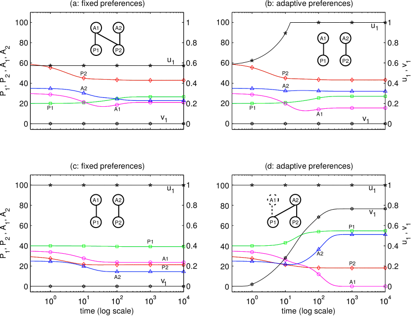
Figure A.1: Dynamics of system (1). Preferences given according to: (a,c) ESS at $t=0$ and kept fixed for $t>0$; (b,d) ESS at all times $(t\geq 0)$. Densities (left axes) represented by $P_{1}$: green squares; $P_{2}$: red diamonds; $A_{1}$: pink circles; $A_{2}$: blue triangles. Plant 1 preferences (right axes) represented by $u_{1}$: 5-pointed, $v_{1}$: 6-pointed stars. Inset graphs display final plant–pollinator interactions (dash stroke for extinct species). Parameters (a,b,c,d): $r_{i}=0.1$, $m_{i}=0.01$, $b_{ij}=0.1$, $a_{i}=0.4$, $w_{i}=0.25$, $e_{11}=e_{22}=0.2$, $d_{1}=0.12,d_{2}=0.1$; (a,b): $K_{i}=50$, $e_{21}=0.17,e_{12}=0.1$; (c,d): $K_{1}=60,K_{2}=30$, $e_{12}=0.17,e_{21}=0.1$. Competition coefficients (a,b): $c_{i}=0.2$; (c,d): $c_{1}=0.4,c_{2}=0.1$.

References

- Aizen et al. (2014) Aizen, M. A., C. L. Morales, D. P. Vázquez, L. A. Garibaldi, A. Sáez, and L. D. Harder (2014). When mutualism goes bad: density-dependent impacts of introduced bees on plant reproduction. New Phytologist 204, 322–328.
- Bascompte and Jordano (2007) Bascompte, J. and P. Jordano (2007). Plant-animal mutualistic networks: the architecture of biodiversity. Annual Review of Ecology Evolution and Systematics 38, 567–593.
- Benadi et al. (2012) Benadi, G., N. Blüthgen, T. Hovestadt, and H.-J. Poethke (2012). Population dynamics of plant and pollinator communities: stability reconsidered. American Naturalist 179, 157–168.
- Bolker et al. (2003) Bolker, B., M. Holyoak, V. Křivan, L. Rowe, and O. Schmitz (2003). Connecting theoretical and empirical studies of trait-mediated interactions. Ecology 84, 1101–1114.
- Boucher (1988) Boucher, D. H. (1988). The Biology of Mutualism: Ecology and Evolution. Oxford University Press.
- Case (2000) Case, T. (2000). An Illustrated Guide to Theoretical Ecology. Oxford University Press.
- Chittka and Schürkens (2001) Chittka, L. and S. Schürkens (2001). Successful invasion of a floral market. Nature 411, 653–653.
- Connell (1980) Connell, J. H. (1980). Diversity and the coevolution of competitors, or the ghost of competition past. Oikos 35, 131–138.
- Feldman et al. (2004) Feldman, T. S., W. F. Morris, and W. G. Wilson (2004). When can two plant species facilitate each other’s pollination? Oikos 105, 197–207.
- Fontaine et al. (2008) Fontaine, C., C. L. Collin, and I. Dajoz (2008). Generalist foraging of pollinators: diet expansion at high density. Journal of Ecology 96, 1002–1010.
- Fontaine et al. (2005) Fontaine, C., I. Dajoz, J. Meriguet, and M. Loreau (2005). Functional diversity of plant–pollinator interaction webs enhances the persistence of plant communities. PLoS Biology 4(1), e1.
- Fretwell and Lucas (1969) Fretwell, S. D. and H. L. Lucas (1969). On territorial behavior and other factors influencing habitat distribution in birds. I. Theoretical development. Acta Biotheoretica 19, 16–36.
- Gause and Witt (1935) Gause, G. F. and A. A. Witt (1935). Behavior of mixed populations and the problem of natural selection. American Naturalist 69, 596–609.
- Gerla and Mooij (2014) Gerla, D. J. and W. M. Mooij (2014). Alternative stable states and alternative endstates of community assembly through intra-and interspecific positive and negative interactions. Theoretical population biology 96, 8–18.
- Geslin et al. (2017) Geslin, B., B. Gauzens, M. Baude, I. Dajoz, C. Fontaine, M. Henry, L. Ropars, O. Rollin, E. Thébault, and N. Vereecken (2017). Massively Introduced Managed Species and Their Consequences for Plant–Pollinator Interactions. Advances in Ecological Research 57, 147–199.
- Grover (1997) Grover, J. P. (1997). Resource Competition. Chapman & Hall.
- Guzmán-Novoa et al. (2010) Guzmán-Novoa, E., L. Eccles, Y. Calvete, J. Mcgowan, P. G. Kelly, and A. Correa-Benítez (2010). Varroa destructor is the main culprit for the death and reduced populations of overwintered honey bee (Apis mellifera) colonies in Ontario, Canada. Apidologie 41, 443–450.
- Hernandez (1998) Hernandez, M. J. (1998). Dynamics of transitions between population interactions: a nonlinear interaction -function defined. Proceedings of the Royal Society B: Biological Sciences 265, 1433–1440.
- Hofbauer and Sigmund (1998) Hofbauer, J. and K. Sigmund (1998). Evolutionary Games and Population Dynamics. Cambridge University Press.
- Holland and DeAngelis (2009) Holland, J. N. and D. L. DeAngelis (2009). Consumer-resource theory predicts dynamic transitions between outcomes of interspecific interactions. Ecology Letters 12, 1357–1366.
- Holland and DeAngelis (2010) Holland, J. N. and D. L. DeAngelis (2010). A consumer-resource approach to the density-dependent population dynamics of mutualism. Ecology 91, 1286–1295.
- Holland et al. (2002) Holland, J. N., D. L. DeAngelis, and J. L. Bronstein (2002). Population dynamics and mutualism: functional responses of benefits and costs. American Naturalist 159, 231–244.
- Jelle Lever et al. (2014) Jelle Lever, J., E. H. van Nes, M. Scheffer, and J. Bascompte (2014). The sudden collapse of pollinator communities. Ecology Letters 17, 350–359.
- Křivan (2003) Křivan, V. (2003). Ideal free distributions when resources undergo population dynamics. Theoretical Population Biology 64, 25–38.
- Křivan et al. (2008) Křivan, V., R. Cressman, and C. Schneider (2008). The ideal free distribution: a review and synthesis of the game-theoretic perspective. Theoretical Population Biology 73, 403–425.
- Křivan and Sirot (2002) Křivan, V. and E. Sirot (2002). Habitat selection by two competing species in a two-habitat environment. American Naturalist 160, 214–234.
- León and Tumpson (1975) León, J. A. and D. B. Tumpson (1975). Competition between two species for two complementary or substitutable resources. Journal of Theoretical Biology 50, 185–201.
- Levin (1970) Levin, S. A. (1970). Community equilibria and stability, and an extension of the competitive exclusion principle. American Naturalist 104, 413–423.
- Maynard Smith and Price (1973) Maynard Smith, J. and G. R. Price (1973). The logic of animal conflict. Nature 246, 15–18.
- Pimm and Rosenzweig (1981) Pimm, S. L. and M. L. Rosenzweig (1981). Competitors and habitat use. Oikos 37, 1–6.
- Pyke (2016) Pyke, G. H. (2016). Plant–pollinator co-evolution: It’s time to reconnect with Optimal Foraging Theory and Evolutionarily Stable Strategies. Perspectives in Plant Ecology, Evolution and Systematics 19, 70–76.
- Revilla (2015) Revilla, T. A. (2015). Numerical responses in resource-based mutualisms: a time scale approach. Journal of Theoretical Biology 378, 39–46.
- Revilla and Křivan (2016) Revilla, T. A. and V. Křivan (2016). Pollinator foraging adaptation and the coexistence of competing plants. PLoS ONE 11, e0160076.
- Rosenzweig (1981) Rosenzweig, M. L. (1981). A theory of habitat selection. Ecology 62, 327–335.
- Schoener (1978) Schoener, T. W. (1978). Effects of density-restricted food encounter on some single-level competition models. Theoretical Population Biology 13, 365–381.
- Traveset and Richardson (2006) Traveset, A. and D. M. Richardson (2006). Biological invasions as disruptors of plant reproductive mutualisms. Trends in Ecology and Evolution 21, 208–216.
- Valdovinos et al. (2016) Valdovinos, F. S., B. J. Brosi, H. M. Briggs, P. Moisset de Espanés, R. Ramos-Jiliberto, and N. D. Martinez (2016). Niche partitioning due to adaptive foraging reverses effects of nestedness and connectance on pollination network stability. Ecology Letters 19, 1277–1286.
- Valdovinos et al. (2013) Valdovinos, F. S., P. Moisset de Espanés, J. D. Flores, and R. Ramos-Jiliberto (2013). Adaptive foraging allows the maintenance of biodiversity of pollination networks. Oikos 122, 907–917.
- Vandermeer and Boucher (1978) Vandermeer, J. and D. H. Boucher (1978). Varieties of mutualistic interaction in population models. Journal of Theoretical Biology 74, 549–558.
- Zhang et al. (2015) Zhang, Z., C. Yan, C. J. Krebs, and N. C. Stenseth (2015). Ecological non-monotonicity and its effects on complexity and stability of populations, communities and ecosystems. Ecological Modelling 312, 374–384.