Arnold-Winther Mixed Finite Elements for Stokes Eigenvalue Problems

Abstract

This paper is devoted to study the Arnold-Winther mixed finite element method for two dimensional Stokes eigenvalue problems using the stress-velocity formulation. A priori error estimates for the eigenvalue and eigenfunction errors are presented. To improve the approximation for both eigenvalues and eigenfunctions, we propose a local post-processing. With the help of the local post-processing, we derive a reliable a posteriori error estimator which is shown to be empirically efficient. We confirm numerically the proven higher order convergence of the post-processed eigenvalues for convex domains with smooth eigenfunctions. On adaptively refined meshes we obtain numerically optimal higher orders of convergence of the post-processed eigenvalues even on nonconvex domains.

Keywords a priori analysis, a posteriori analysis, Arnold-Winther finite element, mixed finite element, Stokes eigenvalue problem

AMS subject classification 65N15, 65N25, 65N30

1 Introduction

Over the last decade, the numerical analysis of the finite element method for eigenvalue problems has been of increasing interest because of various practical applications. Specifically, the numerical analysis of the Stokes eigenvalue problem is a broad research area. Huang et al. [16] discuss the numerical analysis of several stabilized finite element methods for the Stokes eigenvalue problem. In [21], Meddahi et al. proposed a finite element analysis of a pseudo-stress formulation for the Stokes eigenvalue problem. In [25], Türk et al. introduced a stabilized finite element method for two-field and three-field Stokes eigenvalue problems. From [22], one can also study a variety of mixed or hybrid finite element methods for eigenvalue problems.

In the literature, most of the results based on the a posteriori error analysis for the finite element method (see [1, 26] and the references therein) consider the source problem. In comparison there are only a few results for the a posteriori error analysis of the Stokes eigenvalue problem available. In [20], Lovadina et al. presented the numerical analysis for a residual-based a posteriori error estimator for the finite element discretization of the Stokes eigenvalue problem. In [19], Liu et al. proposed the finite element approximation of the Stokes eigenvalue problem based on a projection method, and derive some superconvergence results and the related recovery type a posteriori error estimators. A posteriori error estimators for stabilized low-order mixed finite elements for the Stokes eigenvalue problem are presented by Armentano et al. [2]. A new adaptive mixed finite element method based on residual type a posteriori error estimators for the Stokes eigenvalue problem is proposed by Han et al. [14]. In [15], Huang presented two stabilized finite element methods for the Stokes eigenvalue problem based on the lowest equal-order finite element pair and also discussed a posteriori lower and upper bounds of Stokes eigenvalues.

Arnold and Winther introduced the strongly symmetric Arnold-Winther mixed finite element (MFEM) for linear elastic problems in [3] and proved its stability for any material parameters. Hence, the proposed Arnold-Winther MFEM is also stable for the Stokes problem as a limit case of linear elasticity. In [11], Carstensen et al. presented the Arnold-Winther mixed finite element formulation for the Stokes source problem.

In this paper, we are presenting the Arnold-Winther mixed finite element formulation for the two dimensional Stokes eigenvalue problem using the stress-velocity formulation. In principal, the stress-velocity formulation is originated from a physical model where incompressible Newtonian flows are modeled by the conservation of momentum and the constitute law. The stress-velocity formulation for the Stokes eigenvalue problem reads as follows: find a symmetric stress tensor $\bm{\sigma}$, a nonzero eigenfunction $\bm{u}$, and an eigenvalue $\lambda$ such that

$$-\operatorname{\mathbf{div}}\bm{\sigma} =\lambda\bm{u}\quad\mbox{in}\;\Omega,\quad\mathcal{A}\bm{\sigma}-\bm{\epsilon}(\bm{u})=0\quad\mbox{in}\;\Omega,\quad\bm{u}=0\quad\mbox{on}\;\partial\Omega,$$

for a bounded Lipschitz domain $\Omega\subset\mathbb{R}^{2}$. Here $\bm{\sigma},\mathcal{A}\bm{\sigma}$ and $\bm{\epsilon}(\bm{u})$ are the stress tensor, the deviatoric stress tensor and the deformation rate tensor, respectively.

For simplicity, we restrict ourselves in this paper to the analysis for simple eigenvalues $\lambda$. This simplifies the a priori error analysis in that the eigenspace to $\lambda$ is one-dimensional. Note that the presented a posteriori error estimator can directly be extended to multiple eigenvalues, in the way that the sum over the squared error estimators, for all the discrete eigenvectors that approximate eigenvectors to the same multiple eigenvalue, provides an upper bound of the eigenvalue error.

The remaining parts of this paper are organized as follows: Section 2 presents the necessary notation, the formulation of the problem, the discretization of the domain and the mixed finite element formulation. Section 3 is devoted to study the a priori error analysis of the eigenvalue problem. Section 4 presents the local post-processing and its higher order convergence analysis. The a posteriori error analysis is introduced in Section 5. Finally, we verify the reliability and efficiency of the a posteriori error estimator and the higher order convergence of post-processed eigenvalues in three numerical experiments in Section 6.

2 Preliminaries

Let $H^{s}(\omega)$ be the standard Sobolev space with the associated norm $\|\cdot\|_{s,\omega}$ for $s\geq 0$. In case of $\omega=\Omega$, we use $\|\cdot\|_{s}$ instead of $\|\cdot\|_{s,\Omega}$. Let $H^{-s}(\omega):=(H^{s}(\omega))^{*}$ be the dual space of $H^{s}(\omega)$. Now we extend the definitions for vector and matrix-valued function. Let $\bm{H}^{s}(\omega)=\bm{H}^{s}(\omega;\mathbb{R}^{2})$ and $\bm{H}^{s}(\omega,\mathbb{R}^{2\times 2})$ be the Sobolev spaces over the set of $2$-dimensional vector and $2\times 2$ matrix-valued function, respectively. Define $\bm{v}=(v_{1},v_{2})^{t}\in\mathbb{R}^{2},\bm{\tau}=(\tau_{ij})_{2\times 2}$ and $\bm{\sigma}=(\sigma_{ij})_{2\times 2}\in\mathbb{R}^{2\times 2}$, then

$$\nabla\bm{v} :=\Bigg{(}\begin{array}[]{cc}\frac{\partial v_{1}}{\partial x}&\frac{\partial v_{1}}{\partial y}\\ \frac{\partial v_{2}}{\partial x}&\frac{\partial v_{2}}{\partial y}\end{array}\Bigg{)},\quad\operatorname{\mathbf{div}}(\tau):=\Bigg{(}\begin{array}[]{c}\frac{\partial\tau_{11}}{\partial x}+\frac{\partial\tau_{12}}{\partial y}\\ \frac{\partial\tau_{21}}{\partial x}+\frac{\partial\tau_{22}}{\partial y}\end{array}\Bigg{)},\quad\mbox{tr}\,\bm{\tau}:=\tau_{11}+\tau_{22},$$

$$\bm{\tau\,v} :=\Big{(}\begin{array}[]{c}\tau_{11}v_{1}+\tau_{12}v_{2}\\ \tau_{21}v_{1}+\tau_{22}v_{2}\end{array}\Big{)},\quad\bm{\tau}:\bm{\sigma}:=\sum_{i,j}\tau_{ij}\sigma_{ij},\quad\bm{\delta}:=2\times 2\;\mbox{unit matrix}.$$

Let the divergence conforming stress space $\bm{H}(\operatorname{\mathbf{div}},\Omega,\mathbb{R}^{2\times 2})$ be defined as

$$\bm{H}(\operatorname{\mathbf{div}},\Omega,\mathbb{R}^{2\times 2}):=\{\bm{\tau}\in\bm{L}^{2}(\Omega;\mathbb{R}^{2\times 2})|\operatorname{\mathbf{div}}\bm{\tau}\in\bm{L}^{2}(\Omega)\},$$

equipped with the norm

$$\|\bm{\tau}\|_{\bm{H}(\operatorname{\mathbf{div}},\Omega,\mathbb{R}^{2\times 2})}^{2}:=(\bm{\tau},\bm{\tau})+(\operatorname{\mathbf{div}}\bm{\tau},\operatorname{\mathbf{div}}\bm{\tau}).$$

In this paper, we are using the notation $(\cdot,\cdot)_{\omega}$ for the $\bm{L}^{2}(\omega;\mathbb{R}^{2\times 2})$ inner product $\int_{\omega}\bm{\tau}:\bm{\tau}dx$ as well as the $\bm{L}^{2}(\omega)$ inner product $\int_{\omega}\bm{\tau}\cdot\bm{\tau}dx$. For $w=\Omega$, the notation $(\cdot,\cdot)$ is used instead of $(\cdot,\cdot)_{\Omega}$. The symbols $\lesssim$ and $\gtrsim$ are used throughout the paper to denote inequalities which are valid up to positive constants that are independent of the local mesh size $h$ but may depend on the size of the eigenvalue $\lambda$ and the coefficient $\nu$.

Let $\Omega\subset\mathbb{R}^{2}$ be a bounded and connected Lipschitz domain. Consider the Stokes eigenvalue problem

$$\begin{split}-\nu\bigtriangleup\bm{u}+\nabla p&=\lambda\bm{u}\quad\,\mbox{in }\Omega,\\ \operatorname{div}\bm{u}&=0\quad\quad\mbox{in }\Omega,\\ \bm{u}&=0\quad\quad\mbox{on }\partial\Omega,\end{split}$$ (1)

with the compatibility condition on the pressure

$$\int_{\Omega}p\;dx=0.$$ (2)

Define $\bm{\sigma}=(\sigma_{i,j})_{2\times 2}$ as a stress tensor and the deformation rate tensor as

$$\bm{\epsilon}(\bm{u}):=\frac{1}{2}(\nabla\bm{u}+(\nabla\bm{u})^{t}).$$

From (1) we can derive the stress-velocity-pressure formulation for the Stokes eigenvalue problem, which is the set of original physical equations for incompressible Newtonian flow,

$$-\operatorname{\mathbf{div}}\bm{\sigma} =\lambda\bm{u}\quad\,\mbox{in }\Omega,$$

$$\bm{\sigma}+p\bm{\delta}-2\nu\bm{\epsilon}(\bm{u}) =0\quad\quad\mbox{in }\Omega,$$

$$\operatorname{div}\bm{u} =0\quad\quad\mbox{in }\Omega,$$

$$\bm{u} =0\quad\quad\mbox{on }\partial\Omega.$$

Next, we define the deviatoric operator $\mathcal{A}:\mathbb{S}\rightarrow\mathbb{S}$, where $\mathbb{S}$ is the space of symmetric tensors $\mathbb{S}=\{\bm{\tau}\in\mathbb{R}^{2\times 2}|\bm{\tau}=\bm{\tau}^{t}\}$. Then we can define the deviator $\mathcal{A}\bm{\tau}$ of $\bm{\tau}$ by

$$\mathcal{A}\bm{\tau}:=\frac{1}{2}\big{(}\bm{\tau}-\frac{1}{2}(\mbox{tr}\;\bm{\tau})\bm{\delta}\big{)}\quad\mbox{for all}\;\bm{\tau}\in\mathbb{S}.$$

Here, $\mbox{Ker}(\mathcal{A})=\{q\bm{\delta}\in\mathbb{S}\;|\;q\in\mathbb{R}\}$ and $\mathcal{A}\tau$ is a trace-free tensor. In addition, $\mathcal{A}$ satisfies for all $\bm{\tau},\bm{\sigma}\in\mathbb{S}$ the following properties,

$$(\mathcal{A}\bm{\tau},\bm{\sigma}) =(\bm{\tau},\mathcal{A}\bm{\sigma}),$$

$$(\mathcal{A}\bm{\tau},2\nu\mathcal{A}\bm{\sigma}) =(\mathcal{A}\bm{\sigma},\bm{\tau})=\frac{1}{2\nu}\Big{(}(\bm{\sigma},\bm{\tau})-\frac{1}{2}(\mbox{tr}\;\bm{\sigma},\mbox{tr}\;\bm{\tau})\Big{)},$$

$$\|\mathcal{A}\bm{\tau}\| \leq\frac{1}{2}\|\bm{\tau}\|.$$

Using the deviatoric tensor $\mathcal{A}$, we arrive at the stress-velocity formulation of the Stokes eigenvalue problem

$$\begin{split}-\operatorname{\mathbf{div}}\bm{\sigma}&=\lambda\bm{u}\quad\,\mbox{in }\Omega,\\ \mathcal{A}\bm{\sigma}-\bm{\epsilon}(\bm{u})&=0\quad\quad\mbox{in }\Omega,\\ \bm{u}&=0\quad\quad\mbox{on }\partial\Omega.\end{split}$$ (3)

Using the compatibility condition (2), we have

$$\int_{\Omega}\mbox{tr}\;\bm{\sigma}\,dx=0.$$

Defining $\bm{V}:=\bm{L}^{2}(\Omega)$ and

$$\bm{\Phi}:=\bm{H}(\operatorname{\mathbf{div}},\Omega;\mathbb{S})/\mathbb{R}\sim\Big{\{}\bm{\tau}\in\bm{H}(\operatorname{\mathbf{div}},\Omega,\mathbb{S})|\int_{\Omega}\mbox{tr}\,\bm{\tau}\,dx=0\Big{\}},$$

we can now derive the following weak form for problem (3): find $\bm{\sigma}\in\bm{\Phi}$, $\bm{u}\in\bm{V}$ with $\|\bm{u}\|_{0}=1$, and $\lambda\in\mathbb{R}_{+}$ such that

$$\begin{split}(\mathcal{A}\bm{\sigma},\bm{\tau})+(\operatorname{\mathbf{div}}\bm{\tau},\bm{u})&=0\qquad\qquad\;\mbox{for all}\;\bm{\tau}\in{\bm{\Phi}},\\ (\operatorname{\mathbf{div}}\bm{\sigma},\bm{v})&=-\lambda(\bm{u},\bm{v})\quad\mbox{for all}\;\bm{v}\in{\bm{V}}.\end{split}$$ (4)

Let $\{\mathcal{T}_{h}\}$ denote a family of regular triangulations of $\bar{\Omega}$ into triangles $K$ of diameter $h_{K}$. For each $\mathcal{T}_{h}$, we define $\mathcal{E}_{h}$ as the set of all edges of $\mathcal{T}_{h}$ and $h_{E}$ as the length of the edge $E\in\mathcal{E}_{h}$. Furthermore, let $[\bm{w}]$ denote the jump of $\bm{w}$,

$$[\bm{w}]|_{E}:=(\bm{w}|_{K_{+}})|_{E}-(\bm{w}|_{K_{-}})|_{E}\quad\mbox{if}\quad E=\bar{K}_{+}\cap\bar{K}_{-}.$$

Let $\nabla_{\mathcal{T}_{h}}$ and $\bm{\epsilon}_{\mathcal{T}_{h}}$ denote the piecewise gradient and the piecewise symmetric gradient, i.e. $(\nabla_{\mathcal{T}_{h}}\cdot)|_{K}=\nabla(\cdot|_{K})$ and $(\bm{\epsilon}_{\mathcal{T}_{h}}\cdot)|_{K}=\bm{\epsilon}(\cdot|_{K})$, for all $K\in\mathcal{T}_{h}$.

Finally, we define the following finite element spaces associated with the triangulation $\mathcal{T}_{h}$,

$$AW_{k}(K) :=\{\bm{\tau}\in P_{k+2}(K;\mathbb{S})\;|\;\operatorname{\mathbf{div}}\bm{\tau}\in P_{k}(K;\mathbb{R}^{2})\},$$

$$\bm{\Phi}_{h} :=\{\bm{\tau}\in\bm{\Phi}\;|\;\bm{\tau}|_{K}\in AW_{k}(K)\},$$

$$\bm{{V}}_{h} :=\{\bm{v}\in\bm{L}^{2}(\Omega)\;|\;\bm{v}|_{K}\in P_{k}(K;\mathbb{R}^{2})\}.$$

Here, $AW_{k}(K)$ denotes the Arnold-Winther MFEM of index $k\geq 1$ of [3] and $P_{k}(K)$ denotes the set of all polynomials of total degree up to $k$ on the domain $K$. The space $\Phi_{h}$ consists of all symmetric polynomial matrix fields of degree at most $k+1$ together with the divergence free matrix fields of degree $k+2$. Note that $\bm{\Phi}_{h}\subset\bm{\Phi}$. When $\bm{\tau}_{h}\in\bm{\Phi}_{h}$ we have that $\bm{\tau}_{h}$ has continuous normal components and $\bm{\tau}_{h}$ satisfies $\int_{\Omega}\mbox{tr}\,\bm{\tau}_{h}dx=0$.

The Arnold-Winther MFEM of the Stokes eigenvalue problem becomes the following: find $\bm{\sigma}_{h}\in\bm{\Phi}_{h}$, $\bm{u}_{h}\in\bm{V}_{h}$ with $\|\bm{u_{h}}\|_{0}=1$, and $\lambda_{h}\in\mathbb{R}_{+}$ such that

$$\begin{split}(\mathcal{A}\bm{\sigma}_{h},\bm{\tau}_{h})+(\operatorname{\mathbf{div}}\bm{\tau}_{h},\bm{u}_{h})&=0\qquad\qquad\qquad\!\mbox{for all}\;\bm{\tau}_{h}\in{\bm{\Phi}_{h}},\\ (\operatorname{\mathbf{div}}\bm{\sigma}_{h},\bm{v}_{h})&=-\lambda_{h}(\bm{u}_{h},\bm{v}_{h})\quad\mbox{for all}\;\bm{v}_{h}\in{\bm{V}_{h}}.\end{split}$$ (5)

3 A priori error analysis

Our main aim is to show that the solutions of the Arnold-Winther MFEM of the Stokes eigenvalue problem converge to the solution of the corresponding spectral problem which comes to apply the classical spectral approximation theory presented in [4] to the associated source problem.

Consider the stress-velocity formulation for the associated source problem

$$\begin{split}-\operatorname{\mathbf{div}}\bm{\sigma^{f}}&=\bm{f}\quad\mbox{in}\;\Omega,\\ \mathcal{A}\bm{\sigma^{f}}-\bm{\epsilon}(\bm{u^{f}})&=0\quad\;\mbox{in}\;\Omega,\\ \bm{u^{f}}&=0\quad\;\mbox{on}\;\partial\Omega.\end{split}$$ (6)

Using the compatibility condition (2), we have

$$\int_{\Omega}\mbox{tr}\;\bm{\sigma^{f}}\,dx=0.$$

For the above problem (6) there exist well-known regularity results for convex domains with sufficiently smooth boundary $\partial\Omega$. If $\bm{f}\in\bm{L}^{2}(\Omega)$ then the solution of problem (6) satisfies $\bm{u}\in\bm{H}^{2}(\Omega)\cap\bm{H}^{1}(\bar{\Omega})$, $p\in{H}^{1}(\Omega)/\mathbb{R}$, $\bm{\sigma}\in\bm{H}^{1}(\Omega;\mathbb{S})$, and

$$\|\bm{u}\|_{2}+\|p\|_{1}+\|\bm{\sigma}\|_{1}\leq\|\bm{f}\|_{0}.$$ (7)

Using the well-posedness of problem (6), the operators $S:\bm{V}\rightarrow\bm{\Phi}$ and $T:\bm{V}\rightarrow\bm{V}$ are well defined for any $\bm{f}\in\bm{V}$ such that $S\bm{f}=\bm{\sigma^{f}}$, and $T\bm{f}=\bm{u}^{f}$ are the stress and velocity solutions, respectively.

We now define the following weak form for problem (3): for given $\bm{f}\in\bm{V}$, $(S\bm{f},T\bm{f})\in(\bm{\Phi},\bm{V})$ is the solution of

$$\begin{split}(\mathcal{A}(S\bm{f}),\bm{\tau})+(\operatorname{\mathbf{div}}\bm{\tau},T\bm{f})&=0\qquad\qquad\mbox{for all }\bm{\tau}\in{\bm{\Phi}},\\ (\operatorname{\mathbf{div}}(S\bm{f}),\bm{v})&=-(\bm{f},\bm{v})\quad\,\mbox{for all }\bm{v}\in{\bm{V}}.\end{split}$$ (8)

The above problem (8) has unique solution from the well known inf-sup condition of the mixed formulation and [11, Lemma 2.1].

For the discrete solution operators $S_{h}:\bm{V}\rightarrow\bm{\Phi}_{h}$ and $T_{h}:\bm{V}\rightarrow\bm{V}_{h}$, the Arnold-Winther MFEM of the Stokes source problem becomes the following: find $S_{h}\bm{f}\in\bm{\Phi}_{h}$ and $T_{h}\bm{f}\in\bm{V}_{h}$ such that

$$\begin{split}(\mathcal{A}(S_{h}\bm{f}),\bm{\tau}_{h})+(\operatorname{\mathbf{div}}\bm{\tau}_{h},T_{h}\bm{f})&=0\quad\quad\quad\;\,\mbox{for all}\;\bm{\tau}_{h}\in{\bm{\Phi}_{h}},\\ (\operatorname{\mathbf{div}}(S_{h}\bm{f}),\bm{v}_{h})&=-(\bm{f},\bm{v}_{h})\quad\mbox{for all}\;\bm{v}_{h}\in{\bm{V}_{h}}.\end{split}$$ (9)

From [11], the discrete source problem is well-posed and has a unique solution. From [3] we have the following a priori estimates for $(\bm{\sigma^{f}},\bm{u^{f}})\in(\bm{\Phi}\cap\bm{H}^{k+2}(\Omega;\mathbb{S}))\times\bm{H}^{k+2}(\Omega)$ and $\bm{f}\in\bm{H}^{k}(\Omega)$

$$\|S\bm{f}-S_{h}\bm{f}\|_{0} \lesssim h^{m}\|\bm{\sigma}^{f}\|_{m},\quad 1\leq m\leq k+2,$$ (10)

$$\|\operatorname{\mathbf{div}}(S\bm{f}-S_{h}\bm{f})\|_{0} \lesssim h^{m}\|\operatorname{\mathbf{div}}\bm{\sigma}^{f}\|_{m},\quad 0\leq m\leq k+1,$$ (11)

$$\|T\bm{f}-T_{h}\bm{f}\|_{0} \lesssim h^{m}\|\bm{u}^{f}\|_{m+1},\quad 1\leq m\leq k+1.$$ (12)

Hence, we can state the following convergence results by (10) and (12)

$$\|T-T_{h}\|_{\mathcal{L}(\bm{V},\bm{V})}\rightarrow 0\quad\mbox{if}\quad h\rightarrow 0,$$ (13)

$$\|S-S_{h}\|_{\mathcal{L}(\bm{V},\bm{\Phi})}\rightarrow 0\quad\mbox{if}\quad h\rightarrow 0.$$ (14)

The above results (13) and (14) are equivalent to the convergence of eigenvalues and eigenfunctions. Thus, using the abstract theory from [6, 22] and the a priori results (10) and (12), we have

$$\|\bm{u}-\bm{u}_{h}\|_{0} \lesssim h^{m},\quad 1\leq m\leq k+1,$$ (15)

$$\|\bm{\sigma}-\bm{\sigma}_{h}\|_{0} \lesssim h^{m},\quad 1\leq m\leq k+2.$$ (16)

Note that $p=-tr\,\bm{\sigma}/2$, hence the approximation of the pressure is defined by $p_{h}=-tr\,\bm{\sigma}_{h}/2$ and satisfies the following estimate

$$\|p-p_{h}\|_{0}=\frac{1}{2}\|\mbox{tr}\,\bm{\sigma}-\mbox{tr}\,\bm{\sigma}_{h}\|_{0}\leq\|\bm{\sigma}-\bm{\sigma}_{h}\|_{0}\lesssim h^{m},\;1\leq m\leq k+2.$$

The next lemma establishes a connection between the errors in the eigenvalues and in the eigenfunctions.

Lemma 3.1.

Let $(\bm{\sigma},\bm{u},\lambda)$ and $(\bm{\sigma}_{h},\bm{u}_{h},\lambda_{h})$ be solutions of the continuous eigenvalue problem (4) and the discrete eigenvalue problem (5), respectively. Then, we have the identity

$$\lambda-\lambda_{h}=2\nu\|\mathcal{A}(\bm{\sigma}-\bm{\sigma}_{h})\|^{2}_{0}-\lambda_{h}\|\bm{u}-\bm{u}_{h}\|^{2}_{0}.$$ (17)

Proof.

From (4) and (5), using $(\bm{u},\bm{u})=1$ and $(\bm{u}_{h},\bm{u}_{h})=1$, we have

$$(2\nu\mathcal{A}\bm{\sigma},\mathcal{A}\bm{\sigma}) =\lambda(\bm{u},\bm{u})=\lambda,$$

$$(2\nu\mathcal{A}\bm{\sigma}_{h},\mathcal{A}\bm{\sigma}_{h}) =\lambda_{h}(\bm{u}_{h},\bm{u}_{h})=\lambda_{h},$$

$$(2\nu\mathcal{A}\bm{\sigma},\mathcal{A}\bm{\sigma}_{h}) =\lambda_{h}(\bm{u}_{h},\bm{u}).$$

Moreover, it follows

$$2\nu\|\mathcal{A}(\bm{\sigma}-\bm{\sigma}_{h})\|_{0}^{2} =2\nu(\mathcal{A}(\bm{\sigma}-\bm{\sigma}_{h}),\mathcal{A}(\bm{\sigma}-\bm{\sigma}_{h}))$$

$$=2\nu(\mathcal{A}\bm{\sigma},\mathcal{A}\bm{\sigma})+2\nu(\mathcal{A}\bm{\sigma}_{h},\mathcal{A}\bm{\sigma}_{h})-4\nu(\mathcal{A}\bm{\sigma},\mathcal{A}\bm{\sigma}_{h})$$

$$=\lambda+\lambda_{h}-2\lambda_{h}(\bm{u}_{h},\bm{u}).$$

Then we obtain

$$\lambda-\lambda_{h}=2\nu\|\mathcal{A}(\bm{\sigma}-\bm{\sigma}_{h})\|_{0}^{2}-2\lambda_{h}+2\lambda_{h}(\bm{u}_{h},\bm{u}).$$

Using $\|\bm{u}-\bm{u}_{h}\|^{2}_{0}=2-2(\bm{u}_{h},\bm{u})$ yields

$$\lambda-\lambda_{h}=2\nu\|\mathcal{A}(\bm{\sigma}-\bm{\sigma}_{h})\|_{0}^{2}-\lambda_{h}\|\bm{u}-\bm{u}_{h}\|^{2}_{0}.$$

∎

An immediate consequence of Lemma 3.1 are the following two lemmas.

Lemma 3.2.

For sufficiently smooth $\bm{u}\in\bm{H}^{k+2}(\Omega)$, $\bm{\sigma}\in\bm{H}^{k+2}(\Omega;\mathbb{S})$, the following a priori error estimate holds

$$|\lambda-\lambda_{h}|\lesssim h^{2m},\quad 0\leq m\leq k+1.$$ (18)

Proof.

The assertion follows from (15)–(17). ∎

Lemma 3.3.

For sufficiently smooth $\bm{u}\in\bm{H}^{k+2}(\Omega)$, $\bm{\sigma}\in\bm{H}^{k+2}(\Omega;\mathbb{S})$, the following a priori error estimate holds

$$\|\operatorname{\mathbf{div}}(\bm{\sigma}-\bm{\sigma}_{h})\|_{0}\lesssim h^{m},\quad 0\leq m\leq k+1.$$ (19)

Proof.

From (4) and (5), we have $\operatorname{\mathbf{div}}(\bm{\sigma})=-\lambda\bm{u}$ and $\operatorname{\mathbf{div}}(\bm{\sigma}_{h})=-\lambda_{h}\bm{u}_{h}$. Therefore we get

$$\|\operatorname{\mathbf{div}}(\bm{\sigma}-\bm{\sigma}_{h})\|_{0} =\|\lambda_{h}\bm{u}_{h}-\lambda\bm{u}\|_{0}\leq(\lambda_{h}-\lambda)\|\bm{u}_{h}\|_{0}+\lambda\|\bm{u}_{h}-\bm{u}\|_{0}.$$

The assertion follows from (15)–(17), and $\|\bm{u}_{h}\|_{0}=1$. ∎

Let $\bm{P}_{h}$ denote the $\bm{L}^{2}$ projection onto $\bm{V}_{h}$ with the well known approximation property

$$\|\bm{P}_{h}\bm{v}-\bm{v}\|_{0} \lesssim h^{m}\|\bm{v}\|_{m},\quad\mbox{for all}\;\bm{v}\in\bm{H}^{m}(\Omega).$$ (20)

In the following we relate the discrete eigenfunctions $(\bm{\sigma}_{h},\bm{u}_{h})$ to the discrete approximations $(\bm{\sigma}_{\lambda,h},\bm{u}_{\lambda,h})$ of the associated source problem (9) with right hand side $\bm{f}=\lambda\bm{u}\in\bm{V}$. Then $\bm{\sigma}_{\lambda,h}=\lambda S_{h}\bm{u}$ and $\bm{u}_{\lambda,h}=\lambda T_{h}\bm{u}$ and we have the following lemma.

Lemma 3.4 ([11, Theorem 3.4]).

For sufficiently smooth boundary $\partial\Omega$, $\bm{\sigma}\in\bm{H}^{k+2}(\Omega;\mathbb{S})$, and $\operatorname{\mathbf{div}}\bm{\sigma}\in\bm{H}^{k+1}(\Omega)$, it holds that

$$\|\bm{P}_{h}\bm{u}-\bm{u}_{\lambda,h}\|_{0} \lesssim h^{k+3}(\|\bm{\sigma}\|_{k+2}+\|\operatorname{\mathbf{div}}\bm{\sigma}\|_{k+1}).$$ (21)

Next, we prove a similar estimate for the eigenfunction $\bm{u}_{h}$ which is used in Section 4 to derive an error estimate for the post-processed eigenfunction.

Theorem 3.5.

For sufficiently smooth boundary $\partial\Omega,\bm{\sigma}\in\bm{H}^{k+2}(\Omega;\mathbb{S})$, $\operatorname{\mathbf{div}}\bm{\sigma}\in\bm{H}^{k+1}(\Omega)$, it holds that

$$\|\bm{P}_{h}\bm{u}-\bm{u}_{h}\|_{0} \lesssim h^{k+3}(h^{k-1}+\|\bm{\sigma}\|_{k+2}+\|\operatorname{\mathbf{div}}\bm{\sigma}\|_{k+1}).$$ (22)

The proof of Theorem 3.5 does not follow directly from Lemma 3.4, because the eigenvalue problem does not satisfy an orthogonality condition, i.e. $(\operatorname{\mathbf{div}}(\bm{\sigma}-\bm{\sigma}_{h}),\bm{v}_{h})\neq 0$, therefore we need the following lemma.

Lemma 3.6.

For sufficiently smooth boundary $\partial\Omega$, $\bm{\sigma}\in\bm{H}^{k+2}(\Omega;\mathbb{S})$, and $\operatorname{\mathbf{div}}\bm{\sigma}\in\bm{H}^{k+1}(\Omega)$, the difference between the discrete eigenfunction $\bm{u}_{h}$ and the discrete solution of the associated source problem $\bm{u}_{\lambda,h}$ can be estimated by

$$\|\bm{u}_{\lambda,h}-\bm{u}_{h}\|\lesssim h^{k+3}(h^{k-1}+\|\bm{\sigma}\|_{k+2}+\|\operatorname{\mathbf{div}}\bm{\sigma}\|_{k+1}).$$

Proof.

First we define some relations

$$\lambda T\bm{u}=\bm{u},\quad\lambda_{h}T_{h}\bm{u}_{h}=\bm{u}_{h}\quad\mbox{and}\quad\lambda T_{h}\bm{u}=\bm{u}_{\lambda,h}.$$

Since $\lambda$ is a simple eigenvalue, the eigenspace of the eigenvalue $\lambda$ is spanned by $\bm{u}$. The operator $T:\bm{V}\rightarrow\bm{V}$ is self adjoint. Therefore the orthogonal complement of $\bm{u}$ is a $T$-invariant subspace denoted by $\bm{U}^{\perp,\bm{V}}$. Moreover the eigenvalue $\lambda$ does not belong to the spectrum of $T|_{{\bm{U}^{\perp,\bm{V}}}}$ which is defined as $T|_{{\bm{U}^{\perp,\bm{V}}}}:{\bm{U}^{\perp,\bm{V}}}\rightarrow{\bm{U}^{\perp,\bm{V}}}$. Thus, we can define the following invertible map

$$(I-\lambda T):{\bm{U}^{\perp,\bm{V}}}\rightarrow{\bm{U}^{\perp,\bm{V}}}.$$

Here $(I-\lambda T)^{-1}$ is bounded. Define $\bm{\delta}_{h}:=\bm{u}_{\lambda,h}-\bm{u}_{h}-(\bm{u}_{\lambda,h}-\bm{u}_{h},\bm{u})\bm{u}$. Using $\|\bm{u}\|_{0}=1$, it follows

$$(\bm{\delta}_{h},\bm{u})=(\bm{u}_{\lambda,h}-\bm{u}_{h}-(\bm{u}_{\lambda,h}-\bm{u}_{h},\bm{u})\bm{u},\bm{u})=0.$$

Hence we have

$$\bm{\delta}_{h}\in{\bm{U}^{\perp,\bm{V}}}\quad\mbox{and}\quad\|\bm{\delta}_{h}\|_{0}\lesssim\|(I-\lambda T)\bm{\delta}_{h}\|_{0}.$$

Since $(I-\lambda T)\bm{u}=0$, the following estimate holds

$$\|\bm{\delta}_{h}\|_{0}\lesssim\|(I-\lambda T)(\bm{u}_{\lambda,h}-\bm{u}_{h})\|_{0}.$$ (23)

Moreover, we obtain the following inequality

$$\begin{split}&(I-\lambda T)(\bm{u}_{\lambda,h}-\bm{u}_{h})\\ &\quad=(\lambda_{h}T_{h}-\lambda T)(\bm{u}_{\lambda,h}-\bm{u}_{h})+\bm{u}_{\lambda,h}-\bm{u}_{h}-\lambda_{h}T_{h}(\bm{u}_{\lambda,h}-\bm{u})-\lambda_{h}T_{h}(\bm{u}-\bm{u}_{h})\\ &\quad=(\lambda_{h}T_{h}-\lambda T)(\bm{u}_{\lambda,h}-\bm{u}_{h})+(\lambda-\lambda_{h})T_{h}\bm{u}-\lambda_{h}T_{h}(\bm{u}_{\lambda,h}-\bm{u}).\end{split}$$ (24)

Inserting the result of (24) into (23) and using the triangle inequality, implies

$$\|\bm{\delta}_{h}\|_{0} \lesssim\|(\lambda_{h}T_{h}-\lambda T_{h})(\bm{u}_{\lambda,h}-\bm{u}_{h})\|_{0}+\|(\lambda T_{h}-\lambda T)(\bm{u}_{\lambda,h}-\bm{u}_{h})\|_{0}$$

$$\quad+\|(\lambda-\lambda_{h})T_{h}\bm{u}\|_{0}+\|\lambda_{h}T_{h}(\bm{u}_{\lambda,h}-\bm{u})\|_{0},$$

$$\lesssim\mathcal{I}_{1}+\mathcal{I}_{2}+\mathcal{I}_{3}+\mathcal{I}_{4},$$

where

$$\mathcal{I}_{1} =\|(\lambda_{h}T_{h}-\lambda T_{h})(\bm{u}_{\lambda,h}-\bm{u}_{h})\|_{0},\quad\mathcal{I}_{2}=\|(\lambda T_{h}-\lambda T)(\bm{u}_{\lambda,h}-\bm{u}_{h})\|_{0},$$

$$\mathcal{I}_{3} =\|(\lambda-\lambda_{h})T_{h}\bm{u}\|_{0},\quad\quad\quad\quad\quad\quad\;\;\mathcal{I}_{4}=\|\lambda_{h}T_{h}(\bm{u}_{\lambda,h}-\bm{u})\|_{0}.$$

Using the boundedness of $T_{h}$, the estimates of $\mathcal{I}_{1}$ and $\mathcal{I}_{3}$ read

$$\mathcal{I}_{1} \lesssim|\lambda-\lambda_{h}|\|\bm{u}_{\lambda,h}-\bm{u}_{h}\|_{0}\quad\mbox{and}\quad\mathcal{I}_{3}\lesssim|\lambda-\lambda_{h}|.$$ (25)

Using $\bm{f}=(\bm{u}_{\lambda,h}-\bm{u}_{h})$ in (12) and inserting the regularity result (7), we obtain

$$\mathcal{I}_{2}=\|(\lambda T_{h}-\lambda T)(\bm{u}_{\lambda,h}-\bm{u}_{h})\|_{0}\lesssim\lambda h\|(\bm{u}_{\lambda,h}-\bm{u}_{h})\|_{0}.$$ (26)

Adding and subtracting $T_{h}(\bm{P}_{h}\bm{u})$ in $\mathcal{I}_{4}$ leads to

$$\mathcal{I}_{4}\leq\lambda_{h}\|T_{h}(\bm{u}_{\lambda,h}-\bm{P}_{h}\bm{u})\|_{0}+\lambda_{h}\|T_{h}(\bm{P}_{h}\bm{u}-\bm{u})\|_{0}.$$ (27)

Applying Lemma 3.4 in first term of the estimate (27), implies

$$\|T_{h}(\bm{u}_{\lambda,h}-\bm{P}_{h}\bm{u})\|_{0}\lesssim h^{k+3}(\|\bm{\sigma}\|_{k+2}+\|\operatorname{\mathbf{div}}\bm{\sigma}\|_{k+1}).$$

Note that the second term in the estimate (27) is equal to zero due to definition of $T_{h}$, since the right hand side of problem (9) vanishes for $\bm{f}=\bm{P}_{h}\bm{u}-\bm{u}$. Hence

$$\mathcal{I}_{4}\lesssim\lambda_{h}h^{k+3}(\|\bm{\sigma}\|_{k+2}+\|\operatorname{\mathbf{div}}\bm{\sigma}\|_{k+1}).$$

Using the definition of $\bm{\delta}_{h}$, leads to

$$\|\bm{u}_{\lambda,h}-\bm{u}_{h}\|_{0}\leq\|\bm{\delta}_{h}\|_{0}+\|(\bm{u}_{\lambda,h}-\bm{u}_{h},\bm{u})\bm{u}\|_{0}.$$ (28)

The first term of the estimate (28) is already estimated. To estimate the second term, observe that with $\|\bm{u}\|_{0}=1$, we get

$$\|(\bm{u}_{\lambda,h}-\bm{u}_{h},\bm{u})\bm{u}\|_{0}=|(\bm{u}_{\lambda,h}-\bm{u}_{h},\bm{u})|.$$

Moreover, we have

$$\|(\bm{u}_{\lambda,h}-\bm{u}_{h},\bm{u})\bm{u}\|_{0}\leq|(\bm{u}_{\lambda,h}-\bm{u},\bm{u})|+|(\bm{u}-\bm{u}_{h},\bm{u})|.$$

Since $\|\bm{u}\|_{0}=1$ and $\|\bm{u}_{h}\|_{0}=1$, we get

$$|(\bm{u}-\bm{u}_{h},\bm{u})|=1-(\bm{u}_{h},\bm{u})=\frac{1}{2}\|\bm{u}-\bm{u}_{h}\|_{0}^{2}\lesssim h^{2k+2}.$$ (29)

Next, we estimate $|(\bm{u}_{\lambda,h}-\bm{u},\bm{u})|$. Choosing the test functions $\bm{\tau}=\bm{\sigma}_{\lambda,h}-\bm{\sigma}$ and $\bm{v}=\bm{u}_{\lambda,h}-\bm{u}$ in (4), gives

$$(\mathcal{A}\bm{\sigma},\bm{\sigma}_{\lambda,h}-\bm{\sigma})+(\operatorname{\mathbf{div}}(\bm{\sigma}_{\lambda,h}-\bm{\sigma}),\bm{u}) =0,$$

$$(\operatorname{\mathbf{div}}\bm{\sigma},\bm{u}_{\lambda,h}-\bm{u}) =-\lambda(\bm{u},\bm{u}_{\lambda,h}-\bm{u}).$$

From that, we obtain

$$-\lambda(\bm{u}_{\lambda,h}-\bm{u},\bm{u})=(\operatorname{\mathbf{div}}\bm{\sigma},\bm{u}_{\lambda,h}-\bm{u})+(\mathcal{A}\bm{\sigma},\bm{\sigma}_{\lambda,h}-\bm{\sigma})+(\operatorname{\mathbf{div}}(\bm{\sigma}_{\lambda,h}-\bm{\sigma}),\bm{u}).$$

Moreover, we have

$$\begin{split}-\lambda(\bm{u}_{\lambda,h}-\bm{u},\bm{u})&=(\operatorname{\mathbf{div}}(\bm{\sigma}-\bm{\sigma}_{\lambda,h}),\bm{u}_{\lambda,h}-\bm{u})+(\operatorname{\mathbf{div}}\bm{\sigma}_{\lambda,h},\bm{u}_{\lambda,h}-\bm{u})\\ &\quad+(\mathcal{A}(\bm{\sigma}-\bm{\sigma}_{\lambda,h}),\bm{\sigma}_{\lambda,h}-\bm{\sigma})+(\mathcal{A}\bm{\sigma}_{\lambda,h},\bm{\sigma}_{\lambda,h}-\bm{\sigma})\\ &\quad+(\operatorname{\mathbf{div}}(\bm{\sigma}_{\lambda,h}-\bm{\sigma}),\bm{u}-\bm{u}_{\lambda,h})+(\operatorname{\mathbf{div}}(\bm{\sigma}_{\lambda,h}-\bm{\sigma}),\bm{u}_{\lambda,h}).\end{split}$$ (30)

Choosing $\bm{\tau}_{h}=\bm{\sigma}_{\lambda,h}$, $\bm{v}_{h}=\bm{u}_{\lambda,h}$, $\bm{f}=\lambda\bm{u}$ in (9) and $\bm{\tau}=\bm{\sigma}_{\lambda,h}$, $\bm{v}=\bm{u}_{\lambda,h}$ in (4), and subtracting (4) from (9), we obtain

$$\begin{split}(\mathcal{A}(\bm{\sigma}_{\lambda,h}-\bm{\sigma}),\bm{\sigma}_{\lambda,h})+(\operatorname{\mathbf{div}}\bm{\sigma}_{\lambda,h},\bm{u}_{\lambda,h}-\bm{u})&=0,\\ (\operatorname{\mathbf{div}}(\bm{\sigma}_{\lambda,h}-\bm{\sigma}),\bm{u}_{\lambda,h})&=0.\end{split}$$ (31)

Inserting the result from (31) in (30), implies

$$\begin{split}-\lambda(\bm{u}_{\lambda,h}-\bm{u},\bm{u})&=(\mathcal{A}(\bm{\sigma}-\bm{\sigma}_{\lambda,h}),\bm{\sigma}_{\lambda,h}-\bm{\sigma})+2(\operatorname{\mathbf{div}}(\bm{\sigma}-\bm{\sigma}_{\lambda,h}),\bm{u}_{\lambda,h}-\bm{u})\\ &\lesssim\|\bm{\sigma}-\bm{\sigma}_{\lambda,h}\|^{2}_{0}+\|\operatorname{\mathbf{div}}(\bm{\sigma}-\bm{\sigma}_{\lambda,h})\|^{2}_{0}+\|\bm{u}-\bm{u}_{\lambda,h}\|_{0}^{2}\\ &\lesssim h^{2k+4}\|\bm{\sigma}\|_{k+2}^{2}+h^{2k+2}\|\operatorname{\mathbf{div}}\bm{\sigma}\|_{k+1}^{2}+h^{2k+2}\|\bm{u}\|_{k+2}^{2}\\ &\lesssim h^{2k+2}.\end{split}$$ (32)

Summing up the estimates (25)–(27) and (29), (32), we obtain

$$\|\bm{u}_{\lambda,h}-\bm{u}_{h}\|_{0} \lesssim|\lambda-\lambda_{h}|\|\bm{u}_{\lambda,h}-\bm{u}_{h}\|_{0}+h\|\bm{u}_{\lambda,h}-\bm{u}_{h}\|_{0}+|\lambda-\lambda_{h}|$$

$$\quad+h^{k+3}(\|\bm{\sigma}\|_{k+2}+\|\operatorname{\mathbf{div}}\bm{\sigma}\|_{k+1})+h^{2k+2}.$$

Choosing $h$ small enough and using $|\lambda-\lambda_{h}|\lesssim h^{2k+2}$, the following estimate holds

$$\|\bm{u}_{\lambda,h}-\bm{u}_{h}\|_{0}\lesssim h^{k+3}(h^{k-1}+\|\bm{\sigma}\|_{k+2}+\|\operatorname{\mathbf{div}}\bm{\sigma}\|_{k+1}).$$

∎

Proof of Theorem 3.5.

Combining Lemma 3.4 and 3.6, implies the desired result. ∎

4 Local post-processing

In this section we present an improved approximation of the eigenfunction by a local post-processing similar to the one in [11] for the source problem. Define for $m\geq k+2$

$$\bm{W}^{*}_{h}=\{\bm{v}\in\bm{L}^{2}(\Omega)\;|\;\bm{v}|_{K}\in P_{m}(K;\mathbb{R}^{2})\;\mbox{for all}\;K\in\mathcal{T}_{h}\}.$$

Choose $\bm{u}_{h}^{*}\in\bm{W}^{*}_{h}$ on each $K\in\mathcal{T}_{h}$ with $\bm{P}_{K}=\bm{P}_{h}|_{K}$ as a solution of the system

$$\begin{split}\bm{P}_{K}\bm{u}_{h}^{*}&=\bm{u}_{h},\\ (\bm{\epsilon}(\bm{u}_{h}^{*}),\bm{\epsilon}(\bm{v}))_{K}&=(\mathcal{A}\bm{\sigma}_{h},\bm{\epsilon}(\bm{v}))_{K}\quad\mbox{for all}\;\bm{v}\in(\bm{\delta}-\bm{P}_{K})\bm{W}^{*}_{h}|_{K}.\end{split}$$ (33)

Here, $\bm{u}_{h}^{*}$ is the Riesz representation of the linear functional $(\mathcal{A}\bm{\sigma}_{h},\bm{\epsilon}(\cdot))_{K}$ in the Hilbert space

$$(\bm{\delta}-\bm{P}_{K})\bm{W}^{*}_{h}|_{K}\equiv\{\bm{v}_{m}\in P_{m}(K;\mathbb{R}^{2})|(\bm{v}_{m},\bm{w}_{k})_{K}=0\;\mbox{for all}\;\{\bm{w}_{k}\in P_{k}(K;\mathbb{R}^{2})\},$$

which is equipped with the scalar product $(\bm{\epsilon}(\cdot),\bm{\epsilon}(\cdot))_{K}$. We define the local post-processing on each triangle with Lagrange multiplier $\bm{\mu}_{k}\in P_{k}(K;\mathbb{R}^{2})$ as follows

$$\begin{split}(\bm{\epsilon}(\bm{u}_{h}^{*}),\bm{\epsilon}(\bm{v}_{m}))_{K}+(\bm{\mu}_{k},\bm{v}_{m})_{K}&=(\mathcal{A}\bm{\sigma}_{h},\bm{\epsilon}(\bm{v}_{m}))_{K}\quad\mbox{for all}\;\bm{v}_{m}\in P_{m}(K;\mathbb{R}^{2}),\\ (\bm{u}_{h}^{*},\bm{w}_{k})_{K}&=(\bm{u}_{h},\bm{w}_{k})_{K}\quad\quad\;\;\mbox{for all}\;\bm{w}_{k}\in P_{k}(K;\mathbb{R}^{2}).\end{split}$$ (34)

From Korn’s inequality, we get positive definiteness of $(\bm{\epsilon}(\cdot),\bm{\epsilon}(\cdot))_{K}$ on $(\bm{\delta}-\bm{P}_{K})\bm{W}^{*}_{h}|_{K}$, and since $P_{k}(K;\mathbb{R}^{2})\subset P_{m}(K;\mathbb{R}^{2})$, we obtain

$$\sup_{0\neq\bm{v}_{m}\in P_{m}(K;\mathbb{R}^{2})}\frac{(\bm{v}_{m},\bm{\mu}_{k})_{K}}{\|\bm{v}_{m}\|_{1,K}}\geq C\|\bm{\mu}_{k}\|_{0,K}\quad\mbox{for all}\;\bm{\mu}_{k}\in P_{k}(K;\mathbb{R}^{2}).$$

Hence, there exist unique solutions on each triangle, c.f. [8]. Combining the identity $\mathcal{A}\bm{\sigma}=\bm{\epsilon}(\bm{u})$ and (33), gives the following error identity

$$(\bm{\epsilon}(\bm{u}-\bm{u}_{h}^{*}),\bm{\epsilon}(\bm{v}))_{K}=(\mathcal{A}(\bm{\sigma}-\bm{\sigma}_{h}),\bm{\epsilon}(\bm{v}))_{K}\quad\mbox{for all}\;\bm{v}\in(\bm{\delta}-\bm{P}_{K})\bm{W}^{*}_{h}|_{K}.$$

Theorem 4.1.

With sufficiently smooth boundary $\partial\Omega$, if $\bm{u}\in\bm{H}^{m+1}(\Omega)$, $\bm{\sigma}\in\bm{H}^{k+2}(\Omega;\mathbb{S})$, and $\operatorname{\mathbf{div}}\bm{\sigma}\in\bm{H}^{k+1}(\Omega)$ solve problem (1), then the following estimates hold for the post-processed eigenfunction $\bm{u}^{*}_{h}\in\bm{W}^{*}_{h}$

$$\|\bm{u}-\bm{u}_{h}^{*}\|_{0} \lesssim h^{k+3}(h^{k-1}+\|\bm{\sigma}\|_{k+2}+\|\operatorname{\mathbf{div}}\bm{\sigma}\|_{k+1})+h^{m+1}\|\bm{u}\|_{m+1},$$

$$\|\nabla_{\mathcal{T}_{h}}(\bm{u}-\bm{u}_{h}^{*})\|_{0} \lesssim h^{k+2}(h^{k-1}+\|\bm{\sigma}\|_{k+2}+\|\operatorname{\mathbf{div}}\bm{\sigma}\|_{k+1})+h^{m}\|\bm{u}\|_{m+1}.$$

Proof.

Let $\hat{\bm{u}}$ denote the $\bm{L}^{2}$ projection of $\bm{u}$ onto $\bm{W}^{*}_{h}$. From the triangle inequality we get

$$\|\bm{u}-\bm{u}_{h}^{*}\|_{0}\leq\|\bm{u}-\hat{\bm{u}}\|_{0}+\|\bm{P}_{h}(\hat{\bm{u}}-\bm{u}_{h}^{*})\|_{0}+\|(\bm{\delta}-\bm{P}_{h})(\hat{\bm{u}}-\bm{u}_{h}^{*})\|_{0}.$$ (35)

Applying (20) in first part of the right hand side of (35) leads to

$$\|\bm{u}-\hat{\bm{u}}\|_{0}\lesssim h^{m+1}\|\bm{u}\|_{m+1}\quad\mbox{for all}\quad\bm{u}\in\bm{H}^{m+1}(\Omega).$$ (36)

Using $\bm{P}_{K}\bm{u}^{*}_{h}=\bm{u}_{h}$ on each $K\in\mathcal{T}_{h}$ shows

$$\|\bm{P}_{K}(\hat{\bm{u}}-\bm{u}_{h}^{*})\|_{0,K}=\|\bm{P}_{K}\hat{\bm{u}}-\bm{u}_{h}\|_{0,K}.$$

Here $\bm{V}_{h}\subset\bm{W}^{*}_{h}$, so we can apply the result of Theorem 3.5 to deduce

$$\|\bm{P}_{h}(\hat{\bm{u}}-\bm{u}_{h}^{*})\|_{0}=\|\bm{P}_{h}\bm{u}-\bm{u}_{h}\|_{0}\lesssim h^{k+3}(h^{k-1}+\|\bm{\sigma}\|_{k+2}+\|\operatorname{\mathbf{div}}\bm{\sigma}\|_{k+1}).$$ (37)

The estimates for the last term in (35) are identical to the estimates for the post-processing for the source problem, hence we omit the details and quote the final estimate from the proof of [11, Theorem $4.1$]

$$\|(\bm{\delta}-\bm{P}_{h})(\hat{\bm{u}}-\bm{u}_{h}^{*})\|_{0}\lesssim h^{k+3}(\|\bm{\sigma}\|_{k+2}+\|\operatorname{\mathbf{div}}\bm{\sigma}\|_{k+1})+h^{m+1}\|\bm{u}\|_{m+1}.$$ (38)

Combining (35) with (36)–(38) proves the first estimate.

To prove the second estimate, we use the triangle inequality

$$|\bm{u}-\bm{u}_{h}^{*}|_{1,K}\leq|\bm{u}-\hat{\bm{u}}|_{1,K}+|\bm{P}_{h}(\hat{\bm{u}}-\bm{u}_{h}^{*})|_{1,K}+|(\bm{\delta}-\bm{P}_{h})(\hat{\bm{u}}-\bm{u}_{h}^{*})|_{1,K}.$$

Applying an discrete inverse inequality leads to

$$|\bm{u}-\bm{u}_{h}^{*}|_{1,K}\leq|\bm{u}-\hat{\bm{u}}|_{1,K}+h^{-1}\|\bm{P}_{h}(\hat{\bm{u}}-\bm{u}_{h}^{*})\|_{0,K}+h^{-1}\|(\bm{\delta}-\bm{P}_{h})(\hat{\bm{u}}-\bm{u}_{h}^{*})\|_{0,K}.$$

Combining (37) and (38), with the estimate

$$|\bm{u}-\hat{\bm{u}}|_{1,K}\lesssim h^{m}\|\bm{u}\|_{m+1,K}$$

obtained from interpolation type arguments and inverse estimates as in the proof of [11, Theorem $4.1$], proves the second estimate. ∎

Definition 4.2.

For $(\bm{u}^{*}_{h},\bm{u}^{*}_{h})\neq 0$, we define the post-processed eigenvalue as the value of the Rayleigh quotient of the post-processed eigenfunction

$$\lambda_{h}^{*}:=-\frac{(\operatorname{\mathbf{div}}\bm{\sigma}_{h},\bm{u}^{*}_{h})}{(\bm{u}^{*}_{h},\bm{u}^{*}_{h})}.$$ (39)

Theorem 4.3.

Let $(\bm{\sigma},\bm{u},\lambda)\in(\bm{\Phi}\cap\bm{H}^{k+2}(\Omega;\mathbb{S}))\times\bm{H}^{k+2}(\Omega)\times\mathbb{R}_{+}$ be the solution of (4), with $\|\bm{u}\|_{0}=1$. For sufficiently small $h$, the following a priori estimate for the post-processed eigenvalue $\lambda_{h}^{*}$ holds

$$|\lambda-\lambda_{h}^{*}|\lesssim h^{2k+4}.$$

Proof.

From (4), (5), (34), (39), and $(\bm{u},\bm{u})=1$, we have

$$(2\nu\mathcal{A}\bm{\sigma},\mathcal{A}\bm{\sigma})=\lambda(\bm{u},\bm{u})=\lambda,\quad\textrm{and}\quad(2\nu\mathcal{A}\bm{\sigma}_{h},\mathcal{A}\bm{\sigma}_{h})=\lambda_{h}^{*}(\bm{u}_{h}^{*},\bm{u}_{h}^{*}).$$

Moreover, it follows

$$2\nu\|\mathcal{A}(\bm{\sigma}-\bm{\sigma}_{h})\|_{0}^{2} =2\nu(\mathcal{A}(\bm{\sigma}-\bm{\sigma}_{h}),\mathcal{A}(\bm{\sigma}-\bm{\sigma}_{h}))$$

$$=2\nu(\mathcal{A}\bm{\sigma},\mathcal{A}\bm{\sigma})+2\nu(\mathcal{A}\bm{\sigma}_{h},\mathcal{A}\bm{\sigma}_{h})-4\nu(\mathcal{A}\bm{\sigma},\mathcal{A}\bm{\sigma}_{h})$$

$$=\lambda+\lambda_{h}^{*}(\bm{u}_{h}^{*},\bm{u}_{h}^{*})-2\lambda_{h}^{*}(\bm{u},\bm{u}_{h}^{*})+2(\operatorname{\mathbf{div}}\bm{\sigma}_{h},\bm{u})+2\lambda_{h}^{*}(\bm{u},\bm{u}_{h}^{*}).$$

Therefore we have

$$\lambda-\lambda_{h}^{*}=2\nu\|\mathcal{A}(\bm{\sigma}-\bm{\sigma}_{h})\|_{0}^{2}-\lambda_{h}^{*}-\lambda_{h}^{*}(\bm{u}^{*}_{h},\bm{u}^{*}_{h})+2\lambda_{h}^{*}(\bm{u},\bm{u}_{h}^{*})-2(\operatorname{\mathbf{div}}\bm{\sigma}_{h}+\lambda_{h}^{*}\bm{u}_{h}^{*},\bm{u}).$$

Using $(\bm{u},\bm{u})+(\bm{u}^{*}_{h},\bm{u}^{*}_{h})-2(\bm{u},\bm{u}_{h}^{*})=\|\bm{u}-\bm{u}_{h}^{*}\|^{2}_{0}$, and $(\operatorname{\mathbf{div}}\bm{\sigma}_{h}+\lambda_{h}^{*}\bm{u}_{h}^{*},\bm{u}_{h}^{*})=0$ we get

$$\lambda-\lambda_{h}^{*}= 2\nu\|\mathcal{A}(\bm{\sigma}-\bm{\sigma}_{h})\|_{0}^{2}-\lambda_{h}^{*}\|\bm{u}-\bm{u}_{h}^{*}\|^{2}_{0}-2(\operatorname{\mathbf{div}}\bm{\sigma}_{h}+\lambda_{h}^{*}\bm{u}_{h}^{*},\bm{u}-\bm{u}_{h}^{*}),$$ (40)

which leads to

$$\lambda-\lambda_{h}^{*}= 2\nu\|\mathcal{A}(\bm{\sigma}-\bm{\sigma}_{h})\|_{0}^{2}-\lambda_{h}^{*}\|\bm{u}-\bm{u}_{h}^{*}\|^{2}_{0}-2(\operatorname{\mathbf{div}}\bm{\sigma}_{h}-\operatorname{\mathbf{div}}\bm{\sigma},\bm{u}-\bm{u}_{h}^{*})$$

$$-2(\lambda_{h}^{*}\bm{u}_{h}^{*}-\lambda\bm{u},\bm{u}-\bm{u}_{h}^{*})$$

$$= 2\nu\|\mathcal{A}(\bm{\sigma}-\bm{\sigma}_{h})\|_{0}^{2}-\lambda_{h}^{*}\|\bm{u}-\bm{u}_{h}^{*}\|^{2}_{0}-2(\operatorname{\mathbf{div}}\bm{\sigma}_{h}-\operatorname{\mathbf{div}}\bm{\sigma},\bm{u}-\bm{u}_{h}^{*})$$

$$-2(\lambda_{h}^{*}(\bm{u}_{h}^{*}-\bm{u}),\bm{u}-\bm{u}_{h}^{*})-2((\lambda_{h}^{*}-\lambda)\bm{u},\bm{u}-\bm{u}_{h}^{*})$$

$$= 2\nu\|\mathcal{A}(\bm{\sigma}-\bm{\sigma}_{h})\|_{0}^{2}+\lambda_{h}^{*}\|\bm{u}-\bm{u}_{h}^{*}\|^{2}_{0}+2(\operatorname{\mathbf{div}}(\bm{\sigma}-\bm{\sigma}_{h}),\bm{u}-\bm{u}_{h}^{*})$$

$$+2(\lambda-\lambda_{h}^{*})(\bm{u},\bm{u}-\bm{u}_{h}^{*}).$$

From Cauchy-Schwarz inequality it follows

$$|\lambda-\lambda_{h}^{*}| \lesssim 2\nu\|\mathcal{A}(\bm{\sigma}-\bm{\sigma}_{h})\|^{2}_{0}+\lambda_{h}^{*}\|\bm{u}-\bm{u}_{h}^{*}\|^{2}_{0}+2\|\operatorname{\mathbf{div}}(\bm{\sigma}-\bm{\sigma}_{h})\|_{0}\|\bm{u}-\bm{u}_{h}^{*}\|_{0}$$

$$\quad+2|\lambda-\lambda_{h}^{*}|\|\bm{u}-\bm{u}_{h}^{*}\|_{0}.$$

This results in

$$|\lambda-\lambda_{h}^{*}|\lesssim\|\bm{\sigma}-\bm{\sigma}_{h}\|^{2}_{0}+\|\bm{u}-\bm{u}_{h}^{*}\|^{2}_{0}+\|\operatorname{\mathbf{div}}(\bm{\sigma}-\bm{\sigma}_{h})\|_{0}\|\bm{u}-\bm{u}_{h}^{*}\|_{0}+|\lambda-\lambda_{h}^{*}|^{2}.$$

Using the estimates (16) and (19), and Theorem 4.1, we obtain for $h$ small enough

$$|\lambda-\lambda_{h}^{*}|\lesssim h^{2k+4}.$$

∎

5 A posteriori error analysis

First, we define $\tilde{\bm{u}}_{h}\in\bm{H}=\bm{H}^{1}_{0}(\Omega)$. Here $\tilde{\bm{u}}_{h}$ is closely related to the discontinuous approximation $\bm{u}_{h}^{*}$.

The primal mixed formulation of the Stokes source problem with right hand side $\lambda\bm{u}$ reads as follows: find $\bm{\sigma}\in\bm{L}$ and $\bm{u}\in\bm{H}$ such that

$$\begin{split}-(\bm{\sigma},\bm{\epsilon}(\bm{v}))&=-\lambda(\bm{u},\bm{v})\quad\mbox{for all}\;\bm{v}\in{\bm{H}},\\ (2\nu\mathcal{A}\bm{\sigma},\mathcal{A}\bm{\tau})-(\bm{\tau},\bm{\epsilon}(\bm{u}))&=0\qquad\qquad\;\,\mbox{for all}\;\bm{\tau}\in{\bm{L}}.\end{split}$$ (41)

Following [10, Section 1.3], we have the following lemma

Lemma 5.1.

The operator $A:X\rightarrow X^{*}$, defined for $(\bm{\sigma},\bm{u})\in X:=\bm{L}\times\bm{H}$ by

$$(A(\bm{\sigma},\bm{u}))(\bm{\tau},\bm{v}):=(2\nu\mathcal{A}\bm{\sigma},\mathcal{A}\bm{\tau})-(\bm{\sigma},\bm{\epsilon}(\bm{v}))-(\bm{\tau},\bm{\epsilon}(\bm{u})),$$

is linear, bounded, and bijective.

From the above lemma, we obtain

$$\|\mathcal{A}(\bm{\sigma}-\bm{\sigma}_{h})\|_{0}+\|\bm{\epsilon}(\bm{u}-\tilde{\bm{u}}_{h})\|_{0}\approx\|Res_{L}\|_{\bm{L}^{*}}+\|Res_{H}\|_{\bm{H}^{*}},$$ (42)

for any approximation $(\bm{\sigma}_{h},\tilde{\bm{u}}_{h})\in\bm{L}\times\bm{H}$ of the primal source problem with right hand side $\lambda\bm{u}$, where

$$Res_{H}(\bm{v}) :={\lambda}({\bm{u}},\bm{v})+(\bm{\sigma}_{h},\bm{\epsilon}({\bm{v}}))\qquad\quad\;\mbox{for all}\;\bm{v}\in{\bm{H}},$$

$$Res_{L}(\bm{\tau}) :=(2\nu\mathcal{A}\bm{\sigma}_{h},\mathcal{A}\bm{\tau})-(\bm{\tau},\bm{\epsilon}(\tilde{\bm{u}}_{h}))\quad\mbox{for all}\;\bm{\tau}\in{\bm{L}}.$$

Lemma 5.2.

Let $(\bm{\sigma},\bm{u},\lambda)\in\bm{L}\times\bm{H}\times\mathbb{R}_{+}$ be a solution of (4). Then the approximation $(\bm{\sigma}_{h},\tilde{\bm{u}}_{h})\in\bm{L}\times\bm{H}$ satisfies

$$\|\mathcal{A}(\bm{\sigma}-\bm{\sigma}_{h})\|_{0}+\|\bm{\epsilon}_{\mathcal{T}_{h}}(\bm{u}-\tilde{\bm{u}}_{h})\|_{0}$$

$$\qquad\lesssim\|\mathcal{A}{\bm{\sigma}}_{h}-\bm{\epsilon}(\tilde{\bm{u}}_{h})\|_{K,0}+\Big{(}\sum_{K\in\mathcal{T}_{h}}h_{K}^{2}\|\lambda\bm{u}+\operatorname{\mathbf{div}}\bm{\sigma}_{h}\|^{2}_{0}\Big{)}^{1/2}+\bm{\Theta},$$

with the higher order term

$$\bm{\Theta} :=\lambda_{h}\|\bm{u}-\bm{u}_{h}^{*}\|_{0}+|\lambda-\lambda_{h}|.$$

Proof.

Gauss theorem implies for any $\bm{v}\in\bm{H}$

$$Res_{H}(\bm{v}) =({\lambda}{\bm{u}}+\operatorname{\mathbf{div}}\bm{\sigma}_{h},\bm{v}).$$

Let $\bm{v}_{h}$ denote the Scott-Zhang interpolation [23] of $\bm{v}$, then it holds that

$$Res_{H}(\bm{v})=(\lambda\bm{u}+\operatorname{\mathbf{div}}\bm{\sigma}_{h},\bm{v}-\bm{v}_{h})+(\lambda\bm{u}+\operatorname{\mathbf{div}}\bm{\sigma}_{h},\bm{v}_{h}).$$

For the second term on the right hand side, (5) and (33) show

$$(\lambda\bm{u}+\operatorname{\mathbf{div}}\bm{\sigma}_{h},\bm{v}_{h}) =(\lambda\bm{u}-\lambda_{h}\bm{u}_{h},\bm{v}_{h})=(\lambda\bm{u}-\lambda_{h}\bm{u}^{*}_{h},\bm{v}_{h})$$

$$=(\lambda-\lambda_{h})(\bm{u},\bm{v}_{h})+\lambda_{h}(\bm{u}-\bm{u}_{h}^{*},\bm{v}_{h}).$$

Applying Cauchy-Schwarz inequality, it follows

$$Res_{H}(\bm{v}) \lesssim\left(\sum_{K\in\mathcal{T}_{h}}h_{K}^{2}\|\lambda\bm{u}+\operatorname{\mathbf{div}}\bm{\sigma}_{h}\|^{2}_{K,0}\right)^{1/2}\left(\sum_{K\in\mathcal{T}_{h}}h_{K}^{-2}\|(\bm{v}-\bm{v}_{h})\|^{2}_{K,0}\right)^{1/2}$$

$$\quad+\left(\lambda_{h}\|\bm{u}-\bm{u}_{h}^{*}\|+|\lambda-\lambda_{h}|\right)\|\bm{v}_{h}\|_{0}.$$

Poincare’s inequality, and stability and approximation properties of the Scott-Zhang interpolation show

$$Res_{H}(\bm{v})\lesssim\left(\left(\sum_{K\in\mathcal{T}_{h}}h_{K}^{2}\|\lambda\bm{u}+\operatorname{\mathbf{div}}\bm{\sigma}_{h}\|^{2}_{K,0}\right)^{1/2}+\bm{\Theta}\right)|\bm{v}|_{1}.$$

Finally, $\|Res_{L}\|_{\bm{L}^{*}}$ is estimated as

$$Res_{L}(\bm{\tau})=\int_{\Omega}(\mathcal{A}\bm{\sigma}_{h}-\bm{\epsilon}(\tilde{\bm{u}}_{h})):\bm{\tau}dx\leq\|\mathcal{A}\bm{\sigma}_{h}-\bm{\epsilon}(\tilde{\bm{u}}_{h})\|_{0}\|\bm{\tau}\|_{0}.$$

∎

Now, we present an a posteriori error estimator that involves the discontinuous post-processed approximation

$$\bm{u}_{h}^{*}\in H^{1}(\mathcal{T}_{h}):=\{\bm{v}\in\bm{L}^{2}(\Omega)|\bm{v}|_{T}\in\bm{H}^{1}(T)\;\mbox{for all}\;T\in\mathcal{T}_{h}\}.$$

In the following let $\tilde{\bm{u}}_{h}\in\bm{H}$ be the conforming approximation to $\bm{u}$, that is obtained from the discontinuous post-processed function $\bm{u}_{h}^{*}$ by taking the arithmetic mean value

$$\tilde{\bm{u}}_{h}(z):=\frac{1}{|\{K\in\mathcal{T}_{h}:z\in K\}|}\sum_{K\in\mathcal{T}_{h}:z\in K}\bm{u}_{h}^{*}(z)|_{K}$$

for each vertex and edge degree of freedom in $z\in\mathbb{R}^{2}$. A discrete scaling argument and [17, Theorem 2.2] show

$$\sum_{K\in\mathcal{T}_{h}}h_{K}^{-2}\|\bm{u}_{h}^{*}-\tilde{\bm{u}}_{h}\|_{K,0}^{2}+\sum_{K\in\mathcal{T}_{h}}\|\bm{\epsilon}_{\mathcal{T}_{h}}(\bm{u}_{h}^{*})-\bm{\epsilon}(\tilde{\bm{u}}_{h})\|_{K,0}^{2}\lesssim\sum_{E\in\mathcal{E}_{h}}h_{E}^{-1}\|[\bm{u}_{h}^{*}]\|_{E,0}^{2}.$$ (43)

Theorem 5.3.

Let $(\bm{\sigma},\bm{u},\lambda)\in\bm{L}\times\bm{H}\times\mathbb{R}_{+}$ be a solution of (4). The post-processed eigenfunction $\bm{u}_{h}^{*}\in H^{1}(\mathcal{T}_{h})$ satisfies the following reliability estimate

$$\|\mathcal{A}(\bm{\sigma}-\bm{\sigma}_{h})\|_{0}+\|\bm{\epsilon}_{\mathcal{T}_{h}}(\bm{u}-\bm{u}_{h}^{*})\|_{0} \lesssim\eta+\bm{\Upsilon},$$ (44)

for the a posteriori error estimator

$$\eta^{2}:=\|\mathcal{A}\bm{\sigma}_{h}-\bm{\epsilon}_{\mathcal{T}_{h}}(\bm{u}_{h}^{*})\|^{2}_{0}+\sum_{K\in\mathcal{T}_{h}}h_{K}^{2}\|\lambda^{*}_{h}\bm{u}^{*}_{h}+\operatorname{\mathbf{div}}\bm{\sigma}_{h}\|^{2}_{K,0}+\sum_{E\in\mathcal{E}_{h}}h_{E}^{-1}\|[\bm{u}_{h}^{*}]\|^{2}_{E,0},$$

and the higher order term

$$\bm{\Upsilon}:=\left(\sum_{T\in\mathcal{T}_{h}}h_{K}^{2}\|\lambda\bm{u}-\lambda_{h}^{*}\bm{u}_{h}^{*}\|^{2}_{K,0}\right)^{1/2}+\bm{\Theta}.$$

Proof.

Adding and subtracting $\bm{\epsilon}(\tilde{\bm{u}}_{h})$ in the second term of (44) and using the triangle inequality, we have

$$\|\mathcal{A}(\bm{\sigma}-\bm{\sigma}_{h})\|_{0}+\|\bm{\epsilon}_{\mathcal{T}_{h}}(\bm{u}-\bm{u}_{h}^{*})\|_{0} \lesssim\|\mathcal{A}(\bm{\sigma}-\bm{\sigma}_{h})\|_{0}+\|\bm{\epsilon}_{\mathcal{T}_{h}}(\bm{u}-\tilde{\bm{u}}_{h})\|_{0}$$

$$\quad+\|\bm{\epsilon}_{\mathcal{T}_{h}}(\bm{u}_{h}^{*})-\bm{\epsilon}(\tilde{\bm{u}}_{h})\|_{0}.$$

Applying Theorem 5.2, implies

$$\|\mathcal{A}(\bm{\sigma}-\bm{\sigma}_{h})\|_{0}+\|\bm{\epsilon}_{\mathcal{T}_{h}}(\bm{u}-\bm{u}_{h}^{*})\|_{0} \lesssim\|\mathcal{A}\bm{\sigma}_{h}-\bm{\epsilon}(\tilde{\bm{u}}_{h})\|_{0}+\|\bm{\epsilon}_{\mathcal{T}_{h}}(\bm{u}_{h}^{*})-\bm{\epsilon}(\tilde{\bm{u}}_{h})\|_{0}$$

$$\quad+\left(\sum_{K\in\mathcal{T}_{h}}h_{K}^{2}\|\lambda\bm{u}+\operatorname{\mathbf{div}}\bm{\sigma}_{h}\|^{2}_{K,0}\right)^{1/2}+\bm{\Theta}.$$

Another triangle inequality yields

$$\|\mathcal{A}(\bm{\sigma}-\bm{\sigma}_{h})\|_{0}+\|\bm{\epsilon}_{\mathcal{T}_{h}}(\bm{u}-\bm{u}_{h}^{*})\|_{0} \lesssim\|\mathcal{A}\bm{\sigma}_{h}-\bm{\epsilon}_{\mathcal{T}_{h}}(\bm{u}_{h}^{*})\|_{0}+\|\bm{\epsilon}_{\mathcal{T}_{h}}(\bm{u}_{h}^{*})-\bm{\epsilon}(\tilde{\bm{u}}_{h})\|_{0}$$

$$\quad+\left(\sum_{K\in\mathcal{T}_{h}}h_{K}^{2}\|\lambda^{*}_{h}\bm{u}^{*}_{h}+\operatorname{\mathbf{div}}\bm{\sigma}_{h}\|^{2}_{K,0}\right)^{1/2}+\bm{\Upsilon}.$$

Using (43), the desired estimate holds. ∎

Theorem 5.4.

The a posteriori error estimator $\eta^{2}$ provides an upper bound of the post-processed eigenvalue error for sufficiently small mesh size h, up to the higher order term $\bm{\Upsilon}^{2}$,

$$|\lambda-\lambda^{*}_{h}|\lesssim\eta^{2}+\bm{\Upsilon}^{2}.$$

Proof.

Adding and subtracting $\tilde{\bm{u}}_{h}$ in the last term of (40) yields

$$\lambda-\lambda_{h}^{*} =2\nu\|\mathcal{A}(\bm{\sigma}-\bm{\sigma}_{h})\|_{0}^{2}-\lambda_{h}^{*}\|\bm{u}-\bm{u}_{h}^{*}\|^{2}_{0}-2(\operatorname{\mathbf{div}}\bm{\sigma}_{h}+\lambda_{h}^{*}\bm{u}_{h}^{*},\bm{u}-\tilde{\bm{u}}_{h})$$

$$\quad-2(\operatorname{\mathbf{div}}\bm{\sigma}_{h}+\lambda_{h}^{*}\bm{u}_{h}^{*},\tilde{\bm{u}}_{h}-\bm{u}_{h}^{*})$$

$$=2\nu\|\mathcal{A}(\bm{\sigma}-\bm{\sigma}_{h})\|_{0}^{2}-\lambda_{h}^{*}\|\bm{u}-\bm{u}_{h}^{*}\|^{2}_{0}-2(\bm{\mbox{div}}\bm{\sigma}_{h}-\bm{\mbox{div}}\bm{\sigma},\bm{u}-\tilde{\bm{u}}_{h})$$

$$\quad-2(\lambda_{h}^{*}\bm{u}_{h}^{*}-\lambda\bm{u},\bm{u}-\tilde{\bm{u}}_{h})-2(\operatorname{\mathbf{div}}\bm{\sigma}_{h}+\lambda_{h}^{*}\bm{u}_{h}^{*},\tilde{\bm{u}}_{h}-\bm{u}_{h}^{*}).$$

Applying Gauss theorem, implies

$$\lambda-\lambda_{h}^{*} =2\nu\|\mathcal{A}(\bm{\sigma}-\bm{\sigma}_{h})\|_{0}^{2}+\lambda_{h}^{*}\|\bm{u}-\bm{u}_{h}^{*}\|^{2}_{0}-2(\bm{\sigma}-\bm{\sigma}_{h},\nabla(\bm{u}-\tilde{\bm{u}}_{h}))$$

$$\quad+2\lambda_{h}^{*}(\bm{u}-\bm{u}_{h}^{*},\bm{u}-\tilde{\bm{u}}_{h})+2(\lambda-\lambda_{h}^{*})(\bm{u},\bm{u}-\tilde{\bm{u}}_{h})$$

$$\quad-2(\bm{\mbox{div}}\bm{\sigma}_{h}+\lambda_{h}^{*}\bm{u}_{h}^{*},\tilde{\bm{u}}_{h}-\bm{u}_{h}^{*}).$$

Using Cauchy-Schwarz inequality, we have

$$|\lambda-\lambda_{h}^{*}| \lesssim\|\mathcal{A}(\bm{\sigma}-\bm{\sigma}_{h})\|_{0}^{2}+\|\bm{u}-\bm{u}_{h}^{*}\|^{2}_{0}+\|\bm{\sigma}-\bm{\sigma}_{h}\|_{0}^{2}+\|\nabla(\bm{u}-\tilde{\bm{u}}_{h})\|_{0}^{2}+\|\bm{u}-\tilde{\bm{u}}_{h}\|_{0}^{2}$$

$$\quad+(\lambda-\lambda_{h}^{*})^{2}+\sum_{K\in\mathcal{T}_{h}}h_{K}^{2}\|\lambda_{h}^{*}\bm{u}_{h}^{*}+\operatorname{\mathbf{div}}\bm{\sigma}_{h}\|^{2}_{0,K}+\sum_{K\in\mathcal{T}_{h}}h_{K}^{-2}\|\tilde{\bm{u}}_{h}-\bm{u}_{h}^{*}\|_{0,K}.$$

From the trace estimate [9, Proposition 3.1, IV.3], we get

$$\|\bm{\sigma}-\bm{\sigma}_{h}\|_{0}\lesssim\|\mathcal{A}(\bm{\sigma}-\bm{\sigma}_{h})\|_{0}+\|\operatorname{\mathbf{div}}(\bm{\sigma}-\bm{\sigma}_{h})\|_{-1}.$$

Note that

$$\|\operatorname{\mathbf{div}}(\bm{\sigma}-\bm{\sigma}_{h})\|_{-1}=\sup_{\begin{subarray}{c}\bm{v}\in\bm{H}\\ |\bm{v}|_{1}=1\end{subarray}}|(\lambda\bm{u}+\operatorname{\mathbf{div}}\bm{\sigma}_{h},\bm{v})|=\|Res_{H}\|_{\bm{H}^{*}}.$$

Therefore, (42), Korn’s and triangle inequalities lead to

$$|\lambda-\lambda_{h}^{*}| \lesssim\|\mathcal{A}(\bm{\sigma}-\bm{\sigma}_{h})\|_{0}^{2}+\|\bm{\epsilon}_{\mathcal{T}_{h}}(\bm{u}-\bm{u}_{h}^{*})\|_{0}^{2}+\sum_{K\in\mathcal{T}_{h}}h_{K}^{2}\|\lambda_{h}^{*}\bm{u}_{h}^{*}+\operatorname{\mathbf{div}}\bm{\sigma}_{h}\|^{2}_{0,K}$$

$$\quad+\|\bm{u}_{h}^{*}-\tilde{\bm{u}}_{h}\|^{2}_{0}+\|\bm{\epsilon}_{\mathcal{T}_{h}}(\bm{u}_{h}^{*}-\tilde{\bm{u}}_{h})\|_{0}^{2}+\sum_{K\in\mathcal{T}_{h}}h_{K}^{-2}\|\bm{u}_{h}^{*}-\tilde{\bm{u}}_{h}\|^{2}_{0,K}$$

$$\quad+\|\bm{u}-\bm{u}_{h}^{*}\|^{2}_{0}+(\lambda-\lambda_{h}^{*})^{2}.$$

For $h$ small enough such that $|\lambda-\lambda_{h}^{*}|<1/2$, we conclude with (43) and (44)

$$|\lambda-\lambda_{h}^{*}| \lesssim\eta^{2}+\bm{\Upsilon}^{2}.$$

∎

6 Numerical experiments

In this section, we present numerical results for the square domain, the L-shaped domain and the slit domain. We verify the proven (asymptotic) reliability of the a posteriori error estimator of Section 5 and show empirically its efficiency. We present numerical results that show sixth order convergence of the post-processed eigenvalues of Section 4 on adaptively refined meshes even for the (nonconvex) L-shaped and slit domains. In all experiments, we take to the lowest order Arnold-Winther finite element $(k=1)$, the parameter $\nu=1$ and the polynomial order $P_{3}(\mathcal{T}_{h},\mathbb{R}^{2})$ for the post-processing.

Since the exact eigenvalues for all three domains are unknown, we compare the computed eigenvalues to some reference values with high accuracy. Note that the eigenvalues of the Stokes eigenvalue problem are related to the eigenvalues of the buckling eigenvalue problem of clamped plates via the stream function formulation. Hence, we can use known [5] or computed reference eigenvalues for the plate eigenvalue problem.

We consider the standard adaptive finite element loop

$$\mbox{Solve}\rightarrow\mbox{Estimate}\rightarrow\mbox{Mark}\rightarrow\mbox{Refine},$$

that creates a sequence of adaptively refined (nested) regular meshes $(\mathcal{T_{\ell}})$ level index $\ell$. For the algebraic eigenvalue solver we use the Matlab implementation of ARPACK [18]. To estimate the error, we compute the a posteriori error estimator of Section 5

$$\eta_{\ell}^{2} =\sum_{K\in\mathcal{T}_{\ell}}\|\mathcal{A}\bm{\sigma}_{\ell}-\bm{\epsilon}_{\mathcal{T}_{\ell}}(\bm{u}_{\ell}^{*})\|_{0,K}^{2}+\sum_{E\in\mathcal{E}_{\ell}}h_{E}^{-1}\|[\bm{u}_{\ell}^{*}]\|_{0,E}^{2}+\sum_{K\in\mathcal{T}_{\ell}}h_{K}^{2}\|\lambda^{*}_{\ell}\bm{u}^{*}_{\ell}+\operatorname{\mathbf{div}}\bm{\sigma}_{\ell}\|_{0,K}^{2}.$$

In the above formula, $\bm{u}^{*}_{\ell}\in\bm{W}_{\ell}^{*}$ is the solution of the local post-processing which is given in Section 4. Since the conforming function $\tilde{\bm{u}}_{\ell}$ of Section 5 is closely related to $\bm{u}_{\ell}^{*}$ we also compare the error estimator $\eta_{\ell}^{2}$ to the heuristical estimator

$$\mu_{\ell}^{2} =\sum_{K\in\mathcal{T}_{\ell}}\|\mathcal{A}\bm{\sigma}_{\ell}-\bm{\epsilon}(\tilde{\bm{u}}_{\ell})\|_{0,K}^{2}+\sum_{K\in\mathcal{T}_{\ell}}h_{K}^{2}\|\tilde{\lambda}_{\ell}\tilde{\bm{u}}_{\ell}+\operatorname{\mathbf{div}}\bm{\sigma}_{\ell}\|_{0,K}^{2},$$

where we replaced $\bm{u}_{\ell}^{*}$ by $\tilde{\bm{u}}_{\ell}$, and $\tilde{\lambda}_{\ell}$ is computed from (39) with $\bm{u}_{\ell}^{*}$ replaced by $\tilde{\bm{u}}_{\ell}$. We numerically demonstrate reliability and efficiency of $\mu_{\ell}^{2}$ for the eigenvalue error $|\lambda-\tilde{\lambda}_{\ell}|$. We mark triangles of the triangulation $\mathcal{T}_{\ell}$ in a minimal set of marked triangles $\mathcal{M}_{\ell}$ according to the bulk marking strategy [13], such that $\theta\eta_{\ell}^{2}\leq\eta_{\ell}^{2}(\mathcal{M}_{\ell})$ for the bulk parameter $\theta=1/2$, and refine the mesh with the red-green-blue refinement strategy [26].

Let $N_{\ell}$ denote the degrees of freedom $N_{\ell}:=\mbox{dim}(\bm{\Phi}_{\ell})+\mbox{dim}(\bm{V}_{\ell})$. Note that for uniform meshes, we have the relationship $\mathcal{O}(N_{\ell}^{-r})\approx\mathcal{O}(h_{\ell}^{2r}),\;r>0$.

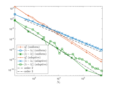
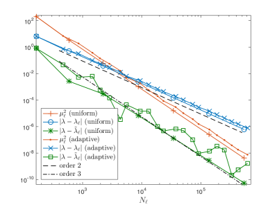
Figure 1: Convergence history of 1 $|\lambda-\lambda_{\ell}|,|\lambda-\lambda_{\ell}^{*}|$, $\eta_{\ell}^{2}$, 1 $|\lambda-\lambda_{\ell}|,|\lambda-\tilde{\lambda}_{\ell}|$ and $\mu_{\ell}^{2}$ on uniformly and adaptively refined meshes for the square domain.

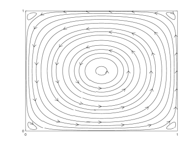
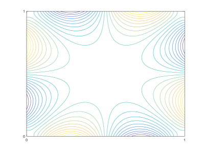
Figure 2: 2 Streamline plot of the discrete eigenfunction $\bm{u}_{\ell}$. 2 Plot of discrete pressure $p_{\ell}=-\mbox{tr}\bm{\sigma}_{\ell}/2$.

6.1 Square domain

In the first example, we consider the square domain $\Omega=(0,1)^{2}$. The reference value for the first eigenvalue $\lambda=52.344691168$ is taken from [5, 12]. Figures 1 and 1 are devoted to the convergence history of the eigenvalue errors and a posteriori error estimators. Due to the smoothness of the eigenfunction, the error of the post-processed eigenvalue $\lambda_{\ell}^{*}$ and the corresponding a posteriori error estimator $\eta_{\ell}^{2}$ achieve optimal third order of convergence for both uniform and adaptive meshes. Moreover, the error for the eigenvalue $\tilde{\lambda}_{\ell}$ and the estimator $\mu_{\ell}^{2}$ also achieve optimal convergence of $\mathcal{O}(N^{-3})$ for both uniform and adaptive meshes. For both uniform and adaptive meshes, the convergence rate of the eigenvalue error of $\lambda_{\ell}$ is equal to $\mathcal{O}(N^{-2})$, which confirms the theoretical result (18). The streamline plot of the discrete eigenfunction $\bm{u}_{\ell}$ and a plot of the discrete pressure $p_{\ell}=-\mbox{tr}\bm{\sigma}_{\ell}/2$ are displayed in 2 and 2, respectively.

6.2 L-shaped domain

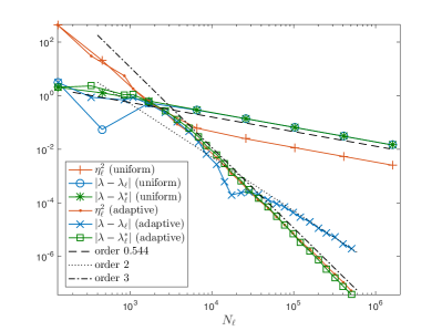
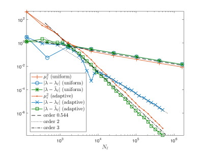
Figure 3: Convergence history of 3 $|\lambda-\lambda_{\ell}|,|\lambda-\lambda_{\ell}^{*}|$, $\eta_{\ell}^{2}$ 3 $|\lambda-\lambda_{\ell}|,|\lambda-\tilde{\lambda}_{\ell}|$ and $\mu_{\ell}^{2}$ on uniformly and adaptively refined meshes for the L-shaped domain.

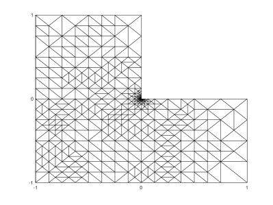
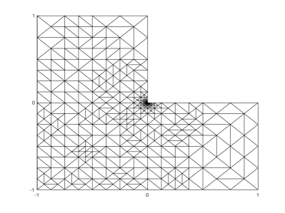
Figure 4: 3 Adaptive refined meshes for $\eta_{\ell}^{2}$ with $386$ nodes, 3 Adaptively refined meshes for $\mu_{\ell}^{2}$ with $392$ nodes.

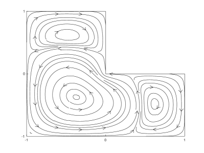
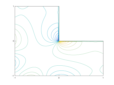
Figure 5: 5Streamline plot of the discrete eigenfunction $\bm{u}_{\ell}$. 5 Plot of discrete pressure $p_{\ell}=-\mbox{tr}\bm{\sigma}_{\ell}/2$.

The second example is for the L-shaped domain with $\Omega=(-1,1)^{2}\setminus[0,1]^{2}$. Here, the domain in nonconvex and has a re-entrant corner at the origin, which causes a singularity in the first eigenfunction. To compute the eigenvalue error of the first eigenvalue, we take $\lambda=32.13269465$ as a reference value, cf. to the values in [7, 24] scaled by $1/4$ due to the differently sized domain. The convergence results for uniform meshes in Figure 3 and 3 show reduced orders of convergence $\mathcal{O}(N^{-0.544})$ for all eigenvalue errors and both error estimators. Furthermore, the convergence results based on adaptive refinement recover optimal higher order convergence $\mathcal{O}(N^{-3})$ of the post-processed eigenvalues $\lambda_{\ell}^{*}$ and $\tilde{\lambda}_{\ell}$. In both cases the corresponding a posteriori error estimators $\eta_{\ell}^{2}$ and $\mu_{\ell}^{2}$ are reliable and efficient and close to the true error. Moreover, the eigenvalue errors for adaptive refinement are several orders of magnitude below the eigenvalue errors for uniform refinement, which illustrates the importance of adaptive mesh refinement. Figures 4 and 4 show two adaptively refined meshes for the a posteriori error estimators $\eta_{\ell}^{2}$ and $\mu_{\ell}^{2}$, respectively. Both meshes show strong refinement toward the origin. Figures 5 and 5 show the discrete velocity and pressure as a streamline plot computed on an adaptive mesh.

6.3 Slit domain

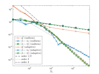
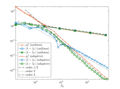
Figure 6: Convergence history of 6 $|\lambda-\lambda_{\ell}|,|\lambda-\lambda_{\ell}^{*}|$, $\eta_{\ell}^{2}$, 6 $|\lambda-\lambda_{\ell}|,|\lambda-\tilde{\lambda}_{\ell}|$ and $\mu_{\ell}^{2}$ on uniformly and adaptively refined meshes for the slit domain.

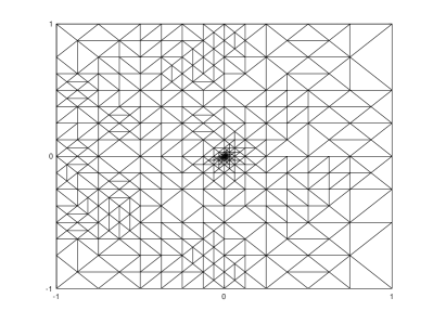
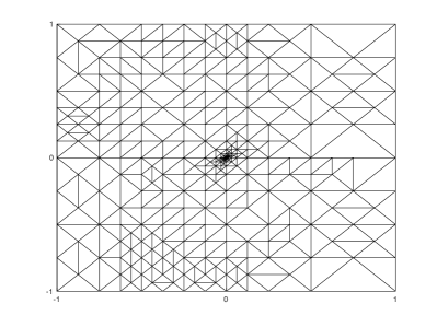
Figure 7: 7 Adaptive refined meshes for $\eta_{\ell}^{2}$ with $375$ nodes, 7 Adaptive refined meshes for $\mu_{\ell}^{2}$ with $336$ nodes.

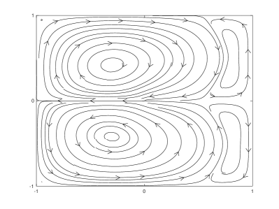
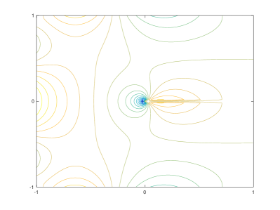
Figure 8: 8Streamline plot of the discrete eigenfunction $\bm{u}_{\ell}$. 8 Plot of discrete pressure $p_{\ell}=-\mbox{tr}\bm{\sigma}_{\ell}/2$.

Finally, we consider the slit domain $\Omega=(-1,1)^{2}\setminus\{0\leq x\leq 1,y=0\}$, with maximal re-entrant corner of angle $2\pi$. We take $\lambda=29.9168629$ as a reference value for the first eigenvalue. Again the first eigenfunction is singular. For uniform meshes in Figure 6 and 6, the convergence results show suboptimal convergence $\mathcal{O}(N^{-1/2})$ for the eigenvalue errors and error estimators. On the contrary, the convergence results, which are based on adaptive refinement, achieve optimal convergence $\mathcal{O}(N^{-3})$ for the post-processed eigenvalues $\lambda_{\ell}^{*}$ and $\tilde{\lambda}_{\ell}$, and for the a posteriori error estimators $\eta_{\ell}^{2}$ and $\mu_{\ell}^{2}$. In Figures 6 and 6, the graphs for the estimators $\eta_{\ell}^{2}$ and $\mu_{\ell}^{2}$ are parallel to the eigenvalue errors of the eigenvalues $\lambda_{\ell}^{*}$ and $\tilde{\lambda}_{\ell}$, thus it confirms that both error estimator are numerically reliable and efficient. Note that the efficiency index corresponding to $\eta_{\ell}^{2}$ in Figure 6 and the efficiency index corresponding $\mu_{\ell}^{2}$ in Figure 6 are close to one in case of adaptive mesh refinement. Figures 7 and 7 display adaptively refined meshes for the proposed error estimators $\eta_{\ell}^{2}$ and $\mu_{\ell}^{2}$, which both show strong refinement toward the re-entrant corner. The computed velocity and discrete pressure are shown in Figures 8 and 8 as a streamline plot on an adaptive mesh.

References

- [1] M. Ainsworth and J. T. Oden. A posteriori error estimation in finite element analysis. Pure and Applied Mathematics (New York). John Wiley & Sons, New York, 2000.
- [2] M. G. Armentano and V. Moreno. A posteriori error estimates of stabilized low-order mixed finite elements for the Stokes eigenvalue problem. J. Comput. Appl. Math., 269:132–149, 2014.
- [3] D. N. Arnold and R. Winther. Mixed finite elements for elasticity. Numer. Math., 92(3):401–419, 2002.
- [4] I. Babuška and J. Osborn. Eigenvalue problems. In Handbook of numerical analysis. Volume II: Finite element methods (Part 1), pages 641–787. Amsterdam etc.: North-Holland, 1991.
- [5] P. E. Bjørstad and B. P. Tjøstheim. High precision solutions of two fourth order eigenvalue problems. Computing, 63(2):97–107, 1999.
- [6] D. Boffi. Finite element approximation of eigenvalue problems. Acta Numer., 19:1–120, 2010.
- [7] S. C. Brenner, P. Monk, and J. Sun. interior penalty Galerkin method for biharmonic eigenvalue problems. In Spectral and high order methods for partial differential equations—ICOSAHOM 2014, volume 106 of Lect. Notes Comput. Sci. Eng., pages 3–15. Springer, Cham, 2015.
- [8] F. Brezzi. On the existence, uniqueness and approximation of saddle-point problems arising from Lagrangian multipliers. Rev. Française Automat. Informat. Recherche Opérationnelle Sér. Rouge, 8(R-2):129–151, 1974.
- [9] F. Brezzi and M. Fortin. Mixed and hybrid finite element methods, volume 15 of Springer Series in Computational Mathematics. Springer-Verlag, New York, 1991.
- [10] C. Carstensen. A unifying theory of a posteriori finite element error control. Numer. Math., 100(4):617–637, 2005.
- [11] C. Carstensen, J. Gedicke, and E.-J. Park. Numerical experiments for the Arnold-Winther mixed finite elements for the Stokes problem. SIAM J. Sci. Comput., 34(4):A2267–A2287, 2012.
- [12] W. Chen and Q. Lin. Approximation of an eigenvalue problem associated with the Stokes problem by the stream function-vorticity-pressure method. Appl. Math., 51(1):73–88, 2006.
- [13] W. Dörfler. A convergent adaptive algorithm for Poisson’s equation. SIAM J. Numer. Anal., 33(3):1106–1124, 1996.
- [14] J. Han, Z. Zhang, and Y. Yang. A new adaptive mixed finite element method based on residual type a posterior error estimates for the Stokes eigenvalue problem. Numer. Methods Partial Differential Equations, 31(1):31–53, 2015.
- [15] P. Huang. Lower and upper bounds of Stokes eigenvalue problem based on stabilized finite element methods. Calcolo, 52(1):109–121, 2015.
- [16] P. Huang, Y. He, and X. Feng. Numerical investigations on several stabilized finite element methods for the Stokes eigenvalue problem. Math. Probl. Eng., pages Art. ID 745908, 14, 2011.
- [17] O. A. Karakashian and F. Pascal. A posteriori error estimates for a discontinuous Galerkin approximation of second-order elliptic problems. SIAM J. Numer. Anal., 41(6):2374–2399, 2003.
- [18] R. Lehoucq, D. Sorensen, and C. Yang. ARPACK Users’ Guide: Solution of Large-Scale Eigenvalue Problems with Implicitly Restarted Arnoldi Methods. Society for Industrial and Applied Mathematics, Philadelphia, PA. USA, 1998.
- [19] H. Liu, W. Gong, S. Wang, and N. Yan. Superconvergence and a posteriori error estimates for the Stokes eigenvalue problems. BIT, 53(3):665–687, 2013.
- [20] C. Lovadina, M. Lyly, and R. Stenberg. A posteriori estimates for the Stokes eigenvalue problem. Numer. Methods Partial Differential Equations, 25(1):244–257, 2009.
- [21] S. Meddahi, D. Mora, and R. Rodríguez. A finite element analysis of a pseudostress formulation for the Stokes eigenvalue problem. IMA J. Numer. Anal., 35(2):749–766, 2015.
- [22] B. Mercier, J. Osborn, J. Rappaz, and P.-A. Raviart. Eigenvalue approximation by mixed and hybrid methods. Math. Comp., 36(154):427–453, 1981.
- [23] L. R. Scott and S. Zhang. Finite element interpolation of nonsmooth functions satisfying boundary conditions. Math. Comp., 54(190):483–493, 1990.
- [24] J. Sun and A. Zhou. Finite element methods for eigenvalue problems. Monographs and Research Notes in Mathematics. CRC Press, Boca Raton, FL, 2017.
- [25] O. Türk, D. Boffi, and R. Codina. A stabilized finite element method for the two-field and three-field Stokes eigenvalue problems. Comput. Methods Appl. Mech. Engrg., 310:886–905, 2016.
- [26] R. Verfürth. A review of a posteriori error estimation and adaptive mesh-refinement techniques. Chichester: John Wiley & Sons; Stuttgart: B. G. Teubner, 1996.