Blockspin renormalization-group study of color confinement due to violation of the non-Abelian Bianchi identity

Abstract

Block-spin transformation of topological defects is applied to the violation of the non-Abelian Bianchi identity (VMABI) on lattice defined as Abelian monopoles. To get rid of lattice artifacts, we introduce 1) smooth gauge fixings such as the maximal center gauge (MCG), 2) block-spin transformations and 3) the tadpole-improved gauge action. The effective action can be determined by adopting the inverse Monte-Carlo method. The coupling constants $F(i)$ of the effective action depend on the coupling of the lattice action $\beta$ and the number of the blocking step $n$. But it is found that $F(i)$ satisfy a beautiful scaling, that is, they are a function of the product $b=na(\beta)$ alone for lattice coupling constants $3.0\leq\beta\leq 3.9$ and the steps of blocking $1\leq n\leq 12$. The effective action showing the scaling behavior can be regarded as an almost perfect action corresponding to the continuum limit, since $a\to 0$ as $n\to\infty$ for fixed $b$. The infrared effective monopole action keeps the global color invariance when smooth gauges such as MCG keeping the invariance are adopted. The almost perfect action showing the scaling is found to be independent of the smooth gauges adopted here as naturally expected from the gauge invariance of the continuum theory. Then we compare the results with those obtained by the analytic blocking method of topological defects from the continuum, assuming local two-point interactions are dominant as the infrared effective action. The action is formulated in the continuum limit while the couplings of these actions can be derived from simple observables calculated numerically on lattices with a finite lattice spacing. When use is made of Berezinskii-Kosterlitz-Thouless (BKT) transformation, the infrared monopole action can be transformed into that of the string model. Since large $b=na(\beta)$ corresponds to the strong-coupling region in the string model, the physical string tension and the lowest glueball mass can be evaluated analytically with the use of the strong-coupling expansion of the string model. The almost perfect action gives us $\sqrt{\sigma}\simeq 1.3\sqrt{\sigma_{phys}}$ for $b\geq 1.0\ \ (\sigma_{phys}^{-1/2})$, whereas the scalar glueball mass is kept to be near $M(0^{++})\sim 3.7\sqrt{\sigma_{phys}}$. In addition, using the effective action composed of simple 10 quadratic interactions alone, we can almost explain analytically the scaling function of the squared monopole density determined numerically for large $b$ region $b>1.2\ (\sigma_{phys}^{-1/2})$.

I Introduction

It is shown in the continuum limit that the violation of the non-Abelian Bianchi identities (VNABI) $J_{\mu}$ is equal to Abelian-like monopole currents $k_{\mu}$ defined by the violation of the Abelian-like Bianchi identities Suzuki:2014wya ; SIB201711 . Although VNABI is an adjoint operator satisfying the covariant conservation rule $D_{\mu}J_{\mu}=0$, it gives us, at the same time, the Abelian-like conservation rule $\partial_{\mu}J_{\mu}=0$. There are $N^{2}-1$ conserved magnetic charges in the case of color $SU(N)$. The charge of each component of VNABI is quantized à la Dirac. The color invariant eigenvalue $\lambda_{\mu}$ of VNABI also satisfies the Abelian conservation rule $\partial_{\mu}\lambda_{\mu}=0$ and the magnetic charge of the eigenvalue is also quantized à la Dirac. If the color invariant eigenvalue make condensation in the QCD vacuum, each color component of the non-Abelian electric field $E^{a}$ is squeezed by the corresponding color component of the sorenoidal current $J^{a}_{\mu}$. Then only the color singlets alone can survive as a physical state and non-Abelian color confinement is realized.

To prove if such a new confinement scheme is realized in nature, studies in the framework of pure $SU(2)$ lattice gauge theories have been done as a simple model of QCD SIB201711 . An Abelian-like definition of a monopole following DeGrand-Toussaint DeGrand:1980eq is adopted as a lattice version of VNABI, since the Dirac quantization condition of the magnetic charge is taken into account on lattice. In Ref SIB201711 , the continuum limit of the lattice VNABI density is studied by introducing various techniques of smoothing the thermalized vacuum which is contaminated by lattice artifacts originally. With these improvements, beautiful and convincing scaling behaviors are seen when we plot the density $\rho(a(\beta),n)$ versus $b=a(\beta)$, where $\rho(a(\beta),n)=\sum_{s,\mu}\sqrt{\sum_{a=1}^{3}(K_{\mu}^{a}(s))^{2}}/(4\sqrt{3}Vb^{3})$, $K_{\mu}^{a}(s)$ is an $n$ blocked monopole in the color direction $a$, $n$ is the number of blocking steps, V is the four-dimensional lattice volume and $b=na(\beta)$ is the lattice spacing of the blocked lattice. A single universal curve $\rho(b)$ is found from $n=1$ up to $n=12$, which suggests that $\rho(a(\beta),n)$ is a function of $b=na(\beta)$ alone. The scaling means that the lattice definition of VNABI has the continuum limit.

The monopole dominance and the dual Meissner effect of the new scheme were studied already several years ago without any gauge fixing Suzuki:2009xy by making use of huge number of thermalized vacua produced by random gauge transformations. The monopole dominance of the string tension was shown beautifully. The dual Meissner effect with respect to each color electric field was shown also beautifully by the Abelian monopole in the corresponding color direction.

Now in this paper we perform the blockspin renormalization-group study of lattice $SU(2)$ gauge theory and try to get the infrared effective VNABI action by introducing a blockspin transformation of lattice VNABI (Abelian monopoles). Since lattice VNABI is defined as Abelian monopoles following Degrand-Toussaint DeGrand:1980eq , the renormalization-group study is similar to the previous works done in maximally Abelian (MA) gauge Ivanenko:1991wt ; Shiba:1994db ; Kato:1998ur ; Chernodub:2000ax . However here we mainly adopt global color-invariant maximal center gauge (MCG) DelDebbio:1996mh ; DelDebbio:1998uu as a gauge smoothing the lattice vacuum, although comparison of the results in other smooth gauges is discussed. Beautiful scaling and gauge-independent behaviors are found to exist, not only with respect to the monopole density done in Ref. SIB201711 , but also with respect to the effective monopole action.

After numerically deriving the infrared effective action with the simple assumption of two-point monopole interactions alone, we try to get the monopole action in the continuum limit by applying the method called blocking from the continuum ref:BFC . When use is made of Berezinskii-Kosterlitz-Thouless (BKT) transformation, the infrared monopole action can be transformed into the string model action. Since large $b=na(\beta)$ corresponds to the strong-coupling region in the string model, the string tension and the lowest glueball mass can be evaluated analytically with the use of the strong-coupling expansion. The almost perfect action gives us $\sqrt{\sigma}\simeq 1.3\sqrt{\sigma_{phys}}$ for $b\geq 1.0\ \ (\sigma_{phys}^{-1/2})$, whereas the lowest scalar glueball mass is kept to be near $M(0^{++})\sim 3.7\sqrt{\sigma}$ Lucini2004 . Finally, we try to explain the scaling behavior of the monopole density observed in Ref. SIB201711 starting from the obtained effective monopole action composed of 10 quadratic interactions alone. Since the square-root operator is difficult to evaluate, we adopt the squared monopole density $R(b)=\sum_{s,\mu}(\sum_{a=1}^{3}(K_{\mu}^{a}(s))^{2})/(4Vb^{3})$. $R(b)$ is found numerically to be a function of $b=na(\beta)$ alone. It is interesting to see the numerically determined scaling behavior of $R(b)$ can almost be reproduced analytically by the simple monopole action for $b>1.2\ (\sigma_{phys}^{-1/2})$, although there remains around 30% discrepancy due mainly to the choice of simplest 10 quadratic monopole interactions alone.

II The effective monopole action and the blockspin transformation of lattice monopoles

The method to derive the monopole action is the following:

• We generate $SU(2)$ link fields $\left\{U(s,\mu)\right\}$ using the tadpole-improved action Alford:1995hw for SU(2) gluodynamics:

  $$S=\beta\sum_{pl}S_{pl}-{\beta\over 20u_{0}^{2}}\sum_{rt}S_{rt}$$ (1)

  where $S_{pl}$ and $S_{rt}$ denote plaquette and $1\times 2$ rectangular loop terms in the action,

  $$S_{pl,rt}\ =\ {1\over 2}{\rm Tr}(1-U_{pl,rt})\,,$$ (2)

  the parameter $u_{0}$ is the input tadpole improvement factor taken here equal to the fourth root of the average plaquette $P=\langle\frac{1}{2}{\mathrm{t}r}U_{pl}\rangle$. We consider $48^{4}$ ($24^{4}$) hyper-cubic lattice for $\beta=3.0\sim 3.9$ (for $\beta=3.0\sim 3.7$). For details of the vacuum generation using the tadpole-improved action, see Ref. SIB201711 .

• Monopole loops in the thermalized vacuum produced from the above improved action (1) still contain large amount of lattice artifacts. Hence we adopt a gauge-fixing technique smoothing the vacuum, although any gauge-fixing is not necessary for smooth continuum configurations. The first smooth gauge is the maximal center gauge DelDebbio:1996mh ; DelDebbio:1998uu which is usually discussed in the framework of the center vortex idea. We adopt the so-called direct maximal center gauge which requires maximization of the quantity

  $$R=\sum_{s,\mu}(\mathop{\rm Tr}U(s,\mu))^{2}$$ (3)

  with respect to local gauge transformations. Here $U(s,\mu)$ is a lattice gauge field. The above condition fixes the gauge up to $Z(2)$ gauge transformation and can be considered as the Landau gauge for the adjoint representation. In our simulations, we choose simulated annealing algorithm as the gauge-fixing method which is known to be powerful for finding the global maximum. For details, see the reference Bornyakov:2000ig .

  For comparison, we also consider the direct Lalacian center gauge(DLCG) Faber:2001zs , Maximal Abelian Wilson loop (AWL) gauge SIB201711 and Maximally Abelian (MA) plus $U1$ Landau gauge(MAU1) Kronfeld:1987ri ; Kronfeld:1987vd ; SIB201711 ; Bali:1996dm .

• Next we perform an abelian projection in the above smooth gauges to separate abelian link variables. We explain how to extract the Abelian fields and the color-magnetic monopoles from the thermalized non-Abelian SU(2) link variables Suzuki:2009xy ,

  $$U(s,\mu)=U^{0}(s,\mu)+i\vec{\sigma}\cdot\vec{U}(s,\mu),$$ (4)

  where $\vec{\sigma}=(\sigma^{1},\sigma^{2},\sigma^{3})$ is the Pauli matrix. Abelian link variables in one of the color directions, for example, in the $\sigma^{1}$ direction are defined as

  $$u_{\mu}(s)=\cos\theta_{\mu}(s)+i\sigma^{1}\sin\theta_{\mu}(s)\;,$$ (5)

  where

  $$\theta^{1}_{\mu}(s)=\arctan\bigl{(}\frac{U^{1}(s,\mu)}{U^{0}(s,\mu)}\bigr{)}\;$$ (6)

  corresponds to the Abelian field.

• Monopole currents can be defined from abelian plaquette variables $\theta_{\mu\nu}^{a}(s)$ following DeGrand and Toussaint DeGrand:1980eq . The abelian plaquette variables are written by

  $$\theta_{\mu\nu}^{a}(s) \equiv \theta_{\mu}^{a}(s)+\theta_{\nu}^{a}(s+\hat{\mu})-\theta_{\mu}^{a}(s+\hat{\nu})-\theta_{\nu}^{a}(s),$$

  $$(-4\pi<\theta_{\mu\nu}^{a}(s)<4\pi).$$

  It is decomposed into two terms:

  $$\theta_{\mu\nu}^{a}(s) \equiv \bar{\theta}_{\mu\nu}^{a}(s)+2\pi{n}_{\mu\nu}^{a}(s),$$

  $$(-\pi\leq\bar{\theta}_{\mu\nu}^{a}(s)<\pi).$$

  Here, $\bar{\theta}_{\mu\nu}^{a}(s)$ is interpreted as the electro-magnetic flux with color $a$ through the plaquette and the integer $n_{\mu\nu}^{a}(s)$ corresponds to the number of Dirac string penetrating the plaquette. One can define quantized conserved monopole currents

  $$k_{\mu}^{a}(s)=\frac{1}{2}\epsilon_{\mu\nu\rho\sigma}\partial_{\nu}n_{\rho\sigma}^{a}(s+\hat{\mu}),$$ (7)

  where $\partial$ denotes the forward difference on the lattice. The monopole currents satisfy a conservation law $\partial^{\prime}_{\mu}k_{\mu}^{a}(s)=0$ by definition, where $\partial^{\prime}$ denotes the backward difference on the lattice.

• We consider a set of independent and local monopole interactions which are summed up over the whole lattice. We denote each operator as ${\cal S}_{i}[k]$. Then the monopole action can be written as a linear combination of these operators:

  $${\cal S}[k]=\sum_{i}F(i){\cal S}_{i}[k],$$ (8)

  where $F(i)$ are coupling constants.

  The effective monopole action is defined as follows:

  $$e^{-{\cal S}[k]} = \int DU(s,\mu)e^{-S(U)}$$

  $$\times\prod_{a}\delta(k_{\mu}^{a}(s)-\frac{1}{2}\epsilon_{\mu\nu\rho\sigma}\partial_{\nu}n_{\rho\sigma}^{a}(s+\hat{\mu})),$$

  where $S(U)$ is the gauge-field action (1).

  We determine the monopole action (8), that is, the set of couplings $F(i)$ from the monopole current ensemble $\left\{k_{\mu}^{a}(s)\right\}$ with the aid of an inverse Monte-Carlo method first developed by Swendsen swendsen and extended to closed monopole currents by Shiba and Suzuki  Shiba:1994db . The details of the inverse Monte-Carlo method are reviewed in AppendixA. See also the previous paper Kato:1998ur .

  Practically, we have to restrict the number of interaction terms. It is natural to assume that monopoles which are far apart do not interact strongly and to consider only short-ranged local interactions of monopoles. The form of actions adopted here are shown in Appendix B and in Appendix C. Some comments are in order:

  • Contrary to previous studies in MA gauge, there are three colored Abelian monopoles here. Due to the possible interactions between gauge fields and monopoles, there may appear interactions between different colored monopoles. When we consider here only effective actions of Abelian monopoles, such induced interactions between monopoles of different colors become jnevitablly non-local. Also no two-point color-mixed interactions appear.

  • We adopt only monopole interactions which are local and have no color mixing, since stable convergence could not be obtained with introduction of color-mixed four and six-point local interactions.

  • Actually, we study here in details assuming two-point monopole interactions alone, although some four and six point interactions without any color mixing are studied for comparison. For the discussions concerning the set of monopole interactios, see Appendix C.

  • All possible types of interactions are not independent due to the conservation law of the monopole current. So we get rid of almost all perpendicular interactions by the use of the conservation rule Shiba:1994db ; Chernodub:2000ax .

• We perform a blockspin transformation in terms of the monopole currents on the dual lattice to investigate the renormalization flow in the IR region. We adopt $n=1,2,3,4,6,8,12$ extended conserved monopole currents as an $n$ blocked operator Ivanenko:1991wt :

  $$K_{\mu}(s^{(n)}) = \sum_{i,j,l=0}^{n-1}k_{\mu}(s(n,i,j,l))$$ (9)

  $$\equiv {\cal B}_{k_{\mu}}(s^{(n)}),$$

  where $s(n,i,j,l)\equiv ns^{(n)}+(n-1)\hat{\mu}+i\hat{\nu}+j\hat{\rho}+l\hat{\sigma}$. The renormalized lattice spacing is $b=na(\beta)$ and the continuum limit is taken as the limit $n\to\infty$ for a fixed physical length $b$.

  We determine the effective monopole action from the blocked monopole current ensemble $\left\{K_{\mu}(s^{(n)})\right\}$. Then one can obtain the renormalization group flow in the coupling constant space.

• The physical length $b=na(\beta)$ is taken in unit of the physical string tension $\sigma_{phys}^{-1/2}$. We evaluate the string tension $\sigma_{lat}$ from the monopole part of the abelian Wilson loops for each $\beta$ since the error bars are small in this case. The lattice spacing $a(\beta)$ is given by the relation $a(\beta)=\sqrt{\sigma_{lat}/\sigma_{phys}}$. Note that $b=1.0\ \sigma_{phys}^{-1/2}$ corresponds to $0.45fm$, when we assume $\sigma_{phys}\cong(440MeV)^{2}$.

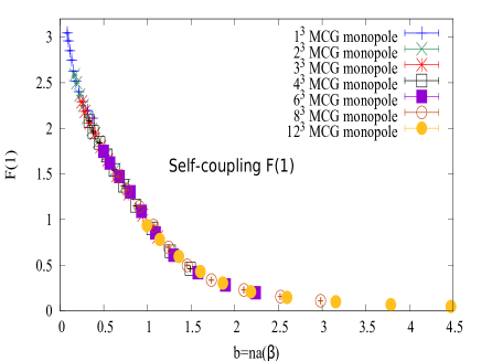
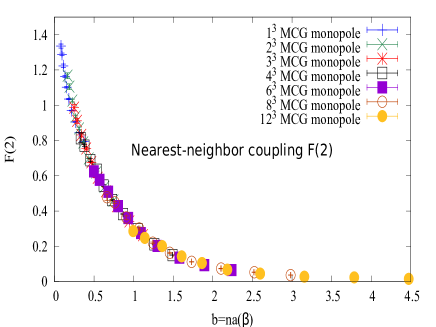
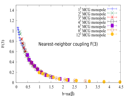
Figure 1: The coupling constants of the self and the two nearest-neighbor interactions in the effective monopole action versus $b=na(\beta)$ in MCG on $48^{4}$.

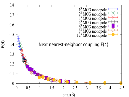
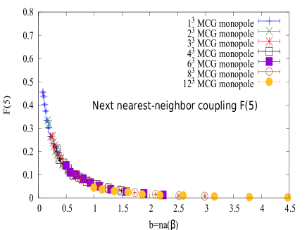
Figure 2: The coupling constants of the two next to the nearest-neighbor interactions in the effective monopole action versus $b=na(\beta)$ in MCG on $48^{4}$.

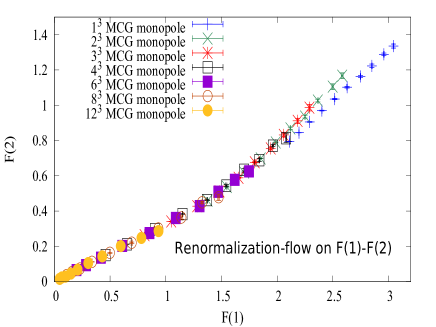
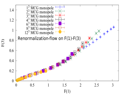
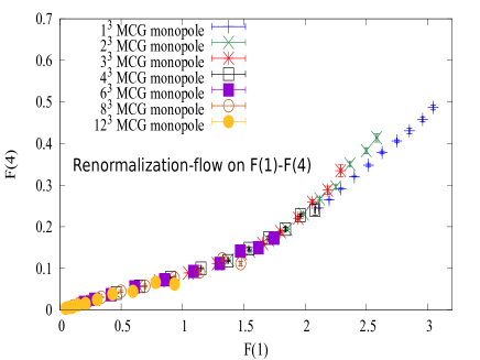
Figure 3: The renoramlization-group flow projected onto the two-dimensional coupling constant planes in MCG on $48^{4}$.

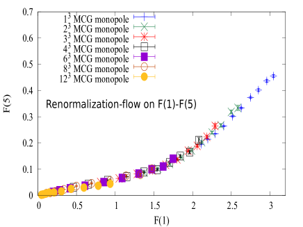
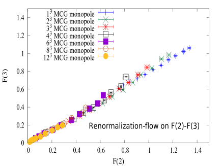
Figure 4: The renoramlization-group flow projected onto the two-dimensional coupling constant planes in MCG on $48^{4}$.

Figure 5: Volume dependence of the infrared effective monopole action in MCG on $24^{4}$ and $48^{4}$. The coupling constants of the self $F(1)$ and the next next nearest-neighbor interactions $F(6)$ are shown as examples.

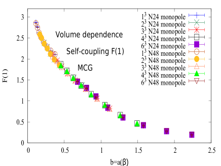
(a) F(1)

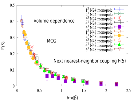
(b) F(6)

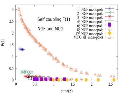
Figure 6: The self coupling of the infrared effective monopole action in NGF case in comparison with that in MCG case.

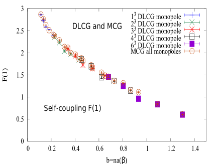
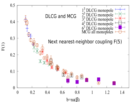
Figure 7: The infrared effective monopole action in DLCG and MCG on $24^{4}$. The coupling constants of the self and the next next nearest-neighbor interactions are shown as an example.

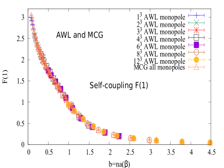
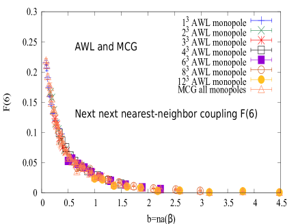
Figure 8: The infrared effective monopole action in AWL and MCG on $48^{4}$. The coupling constants of the self and the next nearest-neighbor interactions are shown as an example.

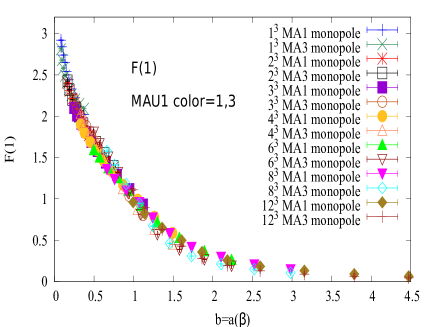
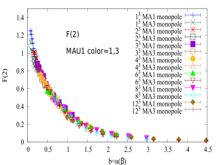
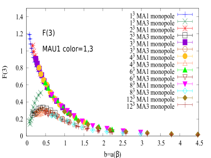
Figure 9: The coupling constants of the self and the two nearest-neighbor interactions in the effective monopole action versus $b=na(\beta)$ in MAU1 on $48^{4}$.

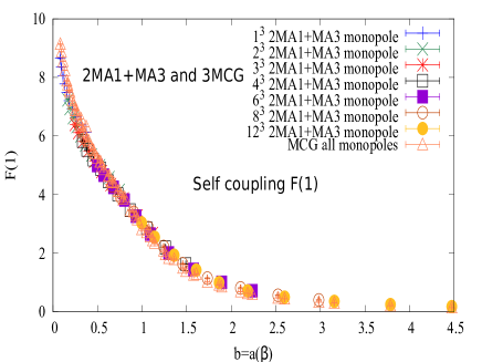
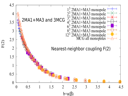
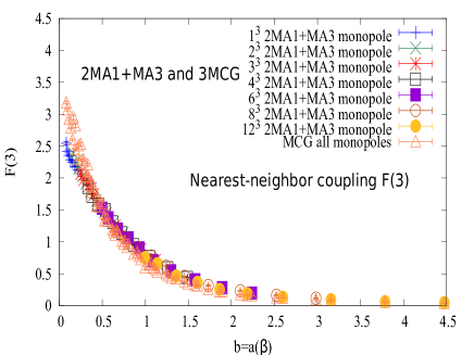
Figure 10: The coupling constants of the self and the nearest-neighbor interactions in the effective monopole action versus $b=na(\beta)$ in MAU1 and MCG on $48^{4}$. The sum of each coupling constants with respect to three color components are shown.

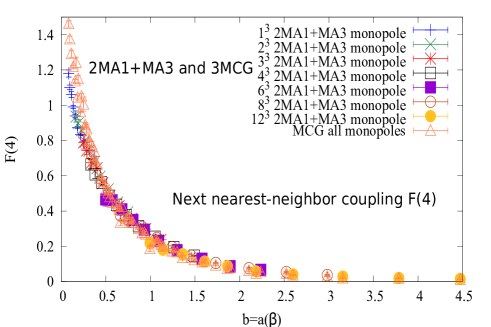
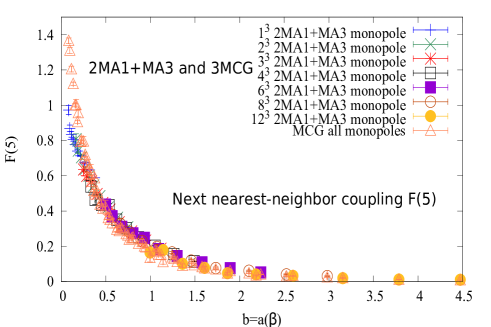
Figure 11: The coupling constants of the two next to the nearest-neighbor interactions in the effective monopole action versus $b=na(\beta)$ in MAU1 and MCG on $48^{4}$. The sum of each coupling constants with respect to three color components are shown.

III Numerical results

As discussed in Appendix B and Appendix C, in the main part of this work, we adopt 10 short-ranged quadratic interactions alone as the form of the effective monopole action for simplicity and also for the comparison with the analytic blocking from the continuum limit.

III.1 Results in MCG gauge on $48^{4}$ lattice

The $10$ coupling constants $F(i)\ (i=1\sim 10)$ of quadratic interactions are fixed very beautifully for lattice coupling constants $3.0\leq\beta\leq 3.9$ and the steps of blocking $1\leq n\leq 12$. Remarkablly they are all expressed by a function of $b=na(\beta)$ alone, although they originally depend on two parameters $\beta$ and $n$. Namely the scaling is satisfied and the continuum limit is obtained when $n\to\infty$ for fixed $b=na(\beta)$. The obtained action can be considered as the projection of the perfect action onto the 10 quadratic coupling constant plane. These behaviors are shown for the first $5$ dominant couplings in Fig.1 and Fig.2. These data are actually much more beautiful than those obtained in previous works in MA gauge considering the third color component alone Chernodub:2000ax .

III.2 Renormalization group flow diagrams

The perfect monopole action draws a unique trajectory in the multi-dimensional coupling-constant space. To see if such a behavior is realized in our case, we plot the renormalization group flow line of our data projected onto some two-dimensional coupling-constant planes in Fig.3 and Fig.4. Except the case for small $b=na(\beta)$ regions especially with $n=1$ case, the unique trajectory is seen clearly. The behaviors are again much more beautiful than those obtained previously in MA gauge Chernodub:2000ax .

III.3 Volume dependence in MCG gauge

Volume dependence is checked in comparison with the data on $24^{4}$ and $48^{4}$ lattices in MCG gauge. Fig. 5 shows examples of the most dominant self-coupling coupling $F(1)$ and the coupling of the next nearest-neighbor interaction $F(5)$. Volume dependence is seen to be small, although the error bars of the data on $24^{4}$ become naturally larger due to the boundary effect when the couplings at larger distances are considered.

III.4 Smooth gauge dependence

The above results are all obtained in MCG gauge. Before studying other smooth gauges, we show the result without any gauge-fixing. In this case, the vacuum is contaminated by dirty artifatcs. Nevertheless, the infrared effective monopole action is determined. Fig.6 shows an example of the coupling of the self-interaction $F(1)$ in comparison with that in MCG gauge. One can see that scaling is not seen at all in NGF case.

III.4.1 DLCG gauge

The direct Lapacian center gauge(DLCG) is a gauge used to study the center vortex Faber:2001zs as MCG. Since DLCG gauge fixing needs more maschine time, we take data on smaller $24^{4}$ lattice only. The results are shown in comparison with those in MCG in Fig.7 with respect to the self-coupling $F(1)$ and the next nearest-neighbor coupling $F(5)$ as an example. Both data are almost equal for the $b=na(\beta)$ regions considered, although small deviations are seen in the $F(5)$ case having the finite-size effects on small $24^{4}$ lattice.

III.4.2 AWL gauge

The third smooth gauge is the maximally Abelian Wilson loop (AWL) gauge Suzuki:1996ax ; SIB201711 , where Abelian $1\times 1$ Wilson loop is maximized as much as possible. The data in AWL is shown in Fig.8 along with those in MCG with respect to the self-coupling $F(1)$ and the next next nearest-neighbor coupling $F(6)$ as an example. The scaling is found very clearly and the both data are almost the same even with respect to $F(6)$ on $48^{4}$ lattice.

III.4.3 MAU1 gauge

Now let us compare MCG and MAU1 gauges, the latter of which is the combination of the maximally Abelian(MA) gauge-fixing Kronfeld:1987vd and Landau gauge fixing with respect to the remaining $U(1)$ Bali:1996dm . In MAU1, the global isospin invariance is broken and the effective action $S(k^{3})$ is different from those of the off-diagonal monopole currents $S(k^{1})$ and $S(k^{2})$. See Fig.9 as an example. With respect to $F(1)$ and $F(2)$, the isospin breaking is not so big, but large deviation is observed with respect to $F(3)$.

However, if the effective actions in both MAU1 and MCG are on the renormalized trajectory corresponding to the continuum limit, the total sum of the monopole actions in three color directions in MAU1 should be equivalent to the sum of three monopole actions in MCG gauge. It is very interesting to see from Fig.10 and Fig.11 that the expectation is realized. Actually except for small $b=na(\beta)$ regions, the gauge-invariance is seen clearly.

III.5 Summary of studies in smooth gauges

From the above data in various gauges, one can conclude that if scaling behaviors are obtained and the effective monopole action is on the renormalized trajectory with the introduction of some smooth gauge fixing, the trajectory obtained becomes universal naturally. In fact, the renormalized trajectory represents the effective action in the continuum limit and gauge dependence should not exist in the continuum. It is exciting to see that this natural expectation is realized actually at least for larger $b$ regions $b\geq 0.5~{}(\sigma_{phys}^{-1/2})$.

Table 1: Best parameters fitted

$b=na(\beta)$	0.5	1	1.5	2	2.5	3	3.5	4	4.5
$\kappa$	0.117504	0.470017	1.057538	1.880067	2.937605	4.230151	5.757705	7.520268	9.51784
$m_{1}$	9	18	27	36	45	54	63	72	81
$m_{2}$	0.9	1.8	2.7	3.6	4.5	5.4	6.3	7.2	8.1
$\bar{\alpha}$	8.682261	2.170565	0.964696	0.542641	0.34729	0.241174	0.177189	0.13566	0.107188
$\bar{\beta}$	6.963001	6.963001	6.963001	6.963001	6.963001	6.963001	6.963001	6.963001	6.963001
$\bar{\gamma}$	1.06e-01	6.63e-03	1.31e-03	4.15e-04	1.70e-04	8.19e-05	4.42e-05	2.59e-05	1.62e-05

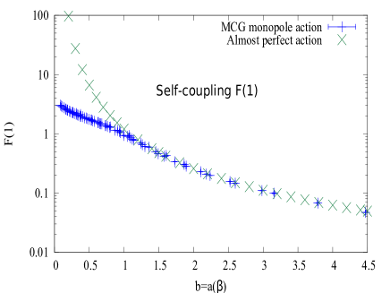
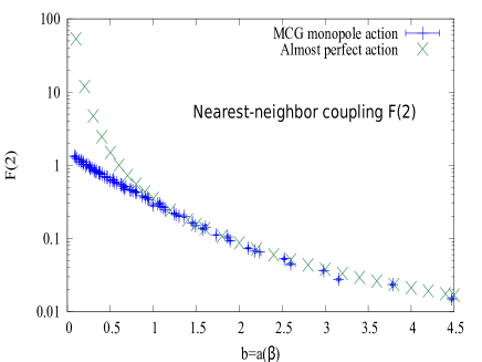
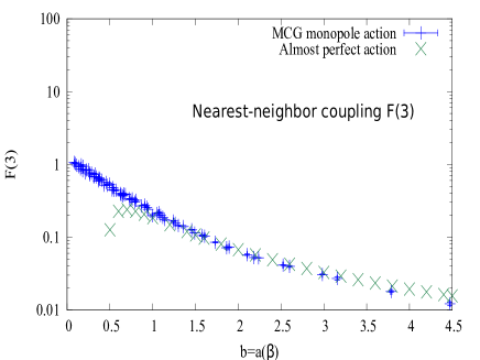
Figure 12: Comparison of the coupling constants of the self and the nearest-neighbor interactions in the effective monopole action between numerical MCG data and theoretical values derived from the almost perfect action.

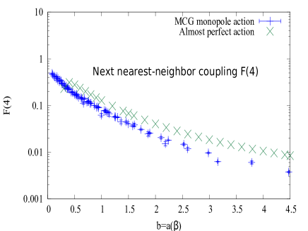
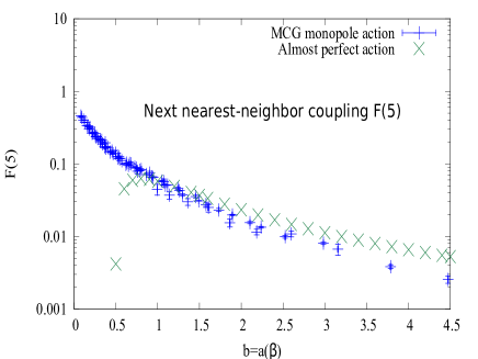
Figure 13: Comparison of the coupling constants of the next nearest-neighbor interactions in the effective monopole action between numerical MCG data and theoretical values derived from the almost perfect action.

IV Blocking from the continuum limit

The infrared effective action determined above numerically shows a clear scaling, that is, a function of $b=na(\beta)$ alone and it can be regarded as an action in the continuum limit. But it is an action still formulated on a lattice with the finite lattice spacing $b=na(\beta)$. Hence various symmetries such as rotational invariance of physical quantities in the continuum limit is difficult to observe, since the action itself does not satisfy, say, the rotational invariance. One has to consider a perfect operator in addition to a perfect action on $b$ lattice in order to reproduce a symmetry such as rotational invariance in the continuum limit Fujimoto:1999ci ; Chernodub:2000ax . For example, a simple Wilson loop on a plane does not reproduce the rotational-invariant static potential on the $b$ lattice.

It is highly desirable to get a perfect action formulated in the continuum space-time which reproduce the same physics at the scale $b$ as those obtained by the above perfect action formulated on the $b$ lattice. If such a perfect action in the continuum space-time is given, the rotational invariance of physical quantities is naturally reproduced with simple operators such as a simple Wilson loop, since the action also respects the invariance.

If the infrared effective monopole action is quadratic, it is possible to perform analytically the blocking from the continuum and to get the infrared monopole action formulated on a coarse $b=na(\beta)$ lattice Fujimoto:1999ci ; Chernodub:2000ax . Perfect operators are also obtained. This is similar to the method developed by Bietenholz and Wiese ref:BFC .

We review the above old works Fujimoto:1999ci ; Chernodub:2000ax shortly. Let us start from the following action composed of quadratic interactions between magnetic monopole currents. It is formulated on an infinite lattice with very small lattice spacing $a$:

$$S[k]=\sum_{s,s^{\prime},\mu}k_{\mu}(s)D_{0}(s-s^{\prime})k_{\mu}(s^{\prime}).$$ (10)

Here we omit the color index. Since we are starting from the region very near to the continuum limit, it is natural to assume the direction independence of $D_{0}(s-s^{\prime})$. Also we adopt only parallel interactions, since we can avoid perpendicular interactions from short-distant terms using the current conservation. Moreover, for simplicity, we adopt only the first three Laurent expansions, i.e., Coulomb, self and nearest-neighbor interactions. Explicitly, $D_{0}(s-s^{\prime})$ is expressed as $\bar{\alpha}\delta_{s,s^{\prime}}+\bar{\beta}\Delta_{L}^{-1}(s-s^{\prime})+\bar{\gamma}\Delta_{L}(s-s^{\prime})$ where $\bar{\alpha},\ \bar{\beta}$ and $\bar{\gamma}$ are free parameters. Here $\Delta_{L}(s-s^{\prime})=-\sum_{\mu}\partial_{\mu}\partial^{\prime}_{\mu}\delta_{s,s^{\prime}}$. Including more complicated quadratic interactions is not difficult.

When we define an operator on the fine $a$ lattice, we can find a perfect operator along the projected flow in the $a\to 0$ limit for fixed $b$. We assume the perfect operator on the projected space as an approximation of the correct operator for the action ${\cal S}[k]$ on the coarse $b$ lattice.

Let us start from

$$\langle W_{m}({\cal C})\rangle = \sum_{k_{\mu}(s)=-\infty\atop{\partial^{\prime}_{\mu}k_{\mu}(s)=0}}^{\infty}\exp\{-\sum_{s,s^{\prime},\mu}k_{\mu}(s)D_{0}(s-s^{\prime})k_{\mu}(s^{\prime})$$ (11)

$$+2\pi i\sum_{s,\mu}N_{\mu}(s)k_{\mu}(s)\}$$

$$\times \prod_{s^{(n)},\mu}\delta\bigg{(}K_{\mu}(s^{(n)})-{\cal B}_{k_{\mu}}(s^{(n)})\bigg{)}/{\cal Z}[k],$$

where ${\cal B}_{k_{\mu}}(s^{(n)})\equiv\sum_{i,j,l=0}^{n-1}k_{\mu}(s(n,i,j,l))~{}($9). Note that the monopole contribution to the static potential is given by the term in Eq.(11)

$$W_{m}({\cal C}) = \exp\bigg{(}2\pi i\sum_{s,\mu}N_{\mu}(s)k_{\mu}(s)\bigg{)},$$

$$N_{\mu}(s) = \sum_{s^{\prime}}\Delta_{L}^{-1}(s-s^{\prime})\frac{1}{2}\epsilon_{\mu\alpha\beta\gamma}\partial_{\alpha}S^{J}_{\beta\gamma}(s^{\prime}+\hat{\mu}),$$ (12)

where $S^{J}_{\beta\gamma}(s^{\prime}+\hat{\mu})$ is a plaquette variable satisfying $\partial^{\prime}_{\beta}S^{J}_{\beta\gamma}(s)=J_{\gamma}(s)$ and the coordinate displacement $\hat{\mu}$ is due to the interaction between dual variables. Here $J_{\mu}(s)$ is an Abelian integer-charged electric current corresponding to an Abelian Wilson loop. See Ref. Chernodub:2000ax .

The cutoff effect of the operator (11) is $O(a)$ by definition. This $\delta$-function renormalization group transformation can be done analytically. Taking the continuum limit $a\to 0$, $n\to\infty$ (with $b=na$ is fixed) finally, we obtain the expectation value of the operator on the coarse lattice with spacing $b=na(\beta)$  Fujimoto:1999ci :

$$\langle W_{m}({\cal C})\rangle = \exp\Biggl{\{}-\pi^{2}\int_{-\infty}^{\infty}\!\!d^{4}xd^{4}y\sum_{\mu}N_{\mu}(x)$$ (13)

$$\times D_{0}^{-1}(x-y)N_{\mu}(y)+\pi^{2}b^{8}\!\!\!\!\sum_{s^{(n)},s^{(n)^{\prime}}\atop{\mu,\nu}}\!\!\!\!B_{\mu}(bs^{(n)})$$

$$\times D_{\mu\nu}(bs^{(n)}-bs^{(n)^{\prime}})B_{\nu}(bs^{(n)^{\prime}})\Biggr{\}}$$

$$\times\!\!\!\!\sum_{b^{3}K_{\mu}(bs)=-\infty\atop\partial^{\prime}_{\mu}K_{\mu}=0}^{\infty}\!\!\!\!\!\!\exp\Biggl{\{}-S[K_{\mu}(s^{(n)})]$$

$$+2\pi ib^{8}\!\!\!\!\sum_{s^{(n)},s^{(n)^{\prime}}\atop{\mu,\nu}}\!\!\!\!B_{\mu}(bs^{(n)})D_{\mu\nu}(bs^{(n)}-bs^{(n)^{\prime}})$$

$$\times K_{\nu}(bs^{(n)^{\prime}})\Biggr{\}}\Bigg{/}\!\!\!\!\sum_{b^{3}K_{\mu}(bs)=-\infty\atop\partial^{\prime}_{\mu}K_{\mu}=0}^{\infty}\!\!\!\!\!\!Z[K,0],$$

where

$$B_{\mu}(bs^{(n)}) \equiv \lim_{a\to 0\atop{n\to\infty}}a^{8}\sum_{s,s^{\prime},\nu}\Pi_{{\neg}\mu}(bs^{(n)}-as)$$ (14)

$$\times \left\{\delta_{\mu\nu}-\frac{\partial_{\mu}\partial^{\prime}_{\nu}}{\sum_{\rho}\partial_{\rho}\partial^{\prime}_{\rho}}\right\}$$

$$\times D_{0}^{-1}(as-as^{\prime})N_{\nu}(as^{\prime}),$$

$$\Pi_{\neg\mu}(bs^{n}-as) \equiv \frac{1}{n^{3}}\delta\left(nas_{\mu}^{(n)}+(n-1)a-as_{\mu}\right)$$

$$\times \prod_{i(\neq\mu)}\left(\sum_{I=0}^{n-1}\delta\left(nas_{i}^{(n)}+Ia-as_{i}\right)\right).$$

$S[K_{\mu}(s^{(n)})]$ denotes the effective action defined on the coarse lattice:

$$S[K_{\mu}(s^{(n)})] = b^{8}\sum_{s^{(n)},s^{(n)^{\prime}}}\sum_{\mu,\nu}K_{\mu}(bs^{(n)})$$ (15)

$$\times D_{\mu\nu}(bs^{(n)}-bs^{(n)^{\prime}})K_{\nu}(bs^{(n)^{\prime}}).$$

Since we take the continuum limit analytically, the operator (13) does not have no cutoff effect. For clarity, we have recovered the scale factor $a$ and $b$ in (13), (14) and (15).

The momentum representation of $D_{\mu\nu}(bs^{(n)}-bs^{(n)^{\prime}})$ takes the form

$$D_{\mu\nu}(p)=A_{\mu\nu}^{GF-1}(p)-\frac{1}{\lambda}\frac{\hat{p_{\mu}}\hat{p_{\nu}}}{(\hat{p}^{2})^{2}}e^{i(p_{\mu}-p_{\nu})/2},$$ (16)

where $\hat{p_{\mu}}=2\sin(p_{\mu}/2)$ and $A_{\mu\nu}^{GF^{-1}}(p)$ is the gauge-fixed inverse of the following operator

$$A^{\prime}_{\mu\nu}(p)\! \equiv \!\left(\prod_{i=1}^{4}\sum_{l_{i}=-\infty}^{\infty}\right)\!\!\Biggl{\{}\!D_{0}^{-1}(p+2\pi l)\Biggl{[}\delta_{\mu\nu}\!$$ (17)

$$-\frac{(p+2\pi l)_{\mu}(p+2\pi l)_{\nu}}{\sum_{i}(p+2\pi l)_{i}^{2}}\Biggr{]}$$

$$\times \frac{(p+2\pi l)_{\mu}(p+2\pi l)_{\nu}}{\prod_{i}(p+2\pi l)_{i}^{2}}\Biggr{\}}\frac{\left(\prod_{i=1}^{4}\hat{p}_{i}\right)^{2}}{\hat{p}_{\mu}\hat{p}_{\nu}}.$$

The explicit form of $D_{\mu\nu}(p)$ is written in Ref. Fujimoto:1999ci . Performing the BKT transformation explained in Appendix B of Ref. Chernodub:2000ax on the coarse lattice, we can get the loop operator for the static potential in the framework of the string model:

$$\langle W_{m}({\cal C})\rangle = \langle W_{m}({\cal C})\rangle_{cl}$$ (18)

$$\times \frac{1}{Z}\!\!\!\!\sum_{\sigma_{\mu\nu}(s)=-\infty\atop{\partial_{[\alpha}\sigma_{\mu\nu]}(s)=0}}^{\infty}\!\!\!\!\exp\Bigg{\{}-\pi^{2}\sum_{s,s^{\prime}\atop{\mu\neq\alpha\atop{\nu\neq\beta}}}\sigma_{\mu\alpha}(s)\partial_{\alpha}\partial_{\beta}^{\prime}$$

$$\times D_{\mu\nu}^{-1}(s-s_{1})\Delta_{L}^{-2}(s_{1}-s^{\prime})\sigma_{\nu\beta}(s^{\prime})$$

$$-2\pi^{2} \sum_{s,s^{\prime}\atop{\mu,\nu}}\sigma_{\mu\nu}(s)\partial_{\mu}\Delta_{L}^{-1}(s-s^{\prime})B_{\nu}(s^{\prime})\Bigg{\}},$$

where $\sigma_{\nu\mu}(s)\equiv\partial_{[\mu}s_{\nu]}$ is the closed string variable satisfying the conservation rule

$$\partial_{[\alpha}\sigma_{\mu\nu]}=\partial_{\alpha}\sigma_{\mu\nu}+\partial_{\mu}\sigma_{\nu\alpha}+\partial_{\nu}\sigma_{\alpha\mu}=0.$$ (19)

The classical part $\langle W_{m}({\cal C})\rangle_{cl}$ is defined by

$$\langle W_{m}({\cal C})\rangle_{cl} = \exp\Bigg{\{}-\pi^{2}\int_{-\infty}^{\infty}\!\!\!\!d^{4}xd^{4}y\sum_{\mu}N_{\mu}(x)$$ (20)

$$\times D_{0}^{-1}(x-y)N_{\mu}(y)\Bigg{\}}.$$

Figure 14: Strong-coupling calculations of the Wilson loops

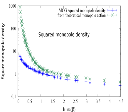
Figure 15: Comparison of monopole density from MCG numrical data and that from the perfect action

V Analytic evaluation of non-perturbative quantities

V.1 Parameter fitting

To derive non-perturbative physical quantites analytically, we have to fix first the propagator $D_{0}(s)$ in (11) of the continuum limit. It can be done by comparing $D_{\mu\nu}^{-1}(s-s^{\prime})$ in Eq.(15) with the set of coupling constants $F(i)\ \ (i=1\sim 10)$ of the monopole action determined numerically in Eq.(8).

$D_{0}(s-s^{\prime})$ in the monopole action (11) is assumed to be $\bar{\alpha}\delta_{s,s^{\prime}}+\bar{\beta}\Delta_{L}^{-1}(s-s^{\prime})+\bar{\gamma}\Delta_{L}(s-s^{\prime})$. We can consider more general quadratic interactions, but as we see later, this choice is almost sufficient to derive the IR region of SU(2) gluodynamics.

The inverse operator of $D_{0}(p)=\bar{\alpha}+\bar{\beta}/p^{2}+\bar{\gamma}p^{2}$ takes the form

$$D_{0}^{-1}(p)=\kappa\left(\frac{m_{1}^{2}}{p^{2}+m_{1}^{2}}-\frac{m_{2}^{2}}{p^{2}+m_{2}^{2}}\right),$$ (21)

where the new parameters $\kappa$, $m_{1}$ and $m_{2}$ satisfy $\kappa(m_{1}^{2}-m_{2}^{2})=\bar{\gamma}^{-1},m_{1}^{2}+m_{2}^{2}=\bar{\alpha}/\bar{\gamma},m_{1}^{2}m_{2}^{2}=\bar{\beta}/\bar{\gamma}$.

Substituting Eq.(21) into Eq.(17) and performing the First Fourier transform(FFT) on a momentum lattice for the several input values $\kappa$, $m_{1}$ and $m_{2}$ we calculate $D_{\mu\nu}(p)$.

To be noted, the three parameters as a function of $b=na(\beta)$ can not be uniquely determined. As shown later, $m_{1}$ ($m_{2}$) corresponds to the inverse of the coherence (penetration) length. Moreover $m_{2}/b$ is found to correpond to the mass of the lowest scalar glueball. Hence we assume

• $m_{1}/m_{2}=10$ for all $b=na(\beta)$ regions.

• $m_{2}/b\sim 1.8$ correponding to $M_{0^{++}}\sim 3.7\sqrt{\sigma_{phys}}$.

• The string tension calculated analytically is as near as possible to the physical string tension $\sigma_{phys}$ and shows scaling, namely $\sigma/\sigma_{phys}$ is constant for all $b=na(\beta)$ regions considered.

Table 1 shows the results of the best fit.

V.2 Comparison of the couplings from numerical analyses and theoretical calculations

Now let us show the coupling constants determined by the analytical blocking method using the above best-fit parameters in Fig.12 and Fig.13. As seen from these figures, the fit is nice for $b=na(\beta)\geq 1.0$, although the deviation becomes larger at smaller $b$ regions, especially for the couplings at larger distace. Note that the logscale is adopted in the $y$ axis.

V.3 The string tension (1)

Let us evaluate the string tension using the perfect operator (18) Fujimoto:1999ci . The plaquette variable $S^{J}_{\alpha\beta}$ in Eq.(12) for the static potential $V(Ib,0,0)$ is expressed by

$$S^{J}_{\alpha\beta}(z) = \delta_{\alpha 1}\delta_{\beta 4}\delta(z_{2})\delta(z_{3})\theta(z_{1})$$ (22)

$$\times \theta(Ib-z_{1})\theta(z_{4})\theta(Tb-z_{4}).$$

We have seen that the monopole action on the dual lattice is in the weak coupling region for large $b$. Then the string model on the original lattice is in the strong coupling region. Therefore, we evaluate Eq.(18) by the strong coupling expansion. The method can be shown diagrammatically in Figure 14.

As explicitly evaluated in Ref. Fujimoto:1999ci , the dominant classical part of the string tension coming from Eq. (20) is

$$\sigma_{cl}=\frac{\pi\kappa}{2b^{2}}\ln\frac{m_{1}}{m_{2}}.$$ (23)

This is consistent with the analytical results suzu89 in Type-2 superconductor. The two constants $m_{1}$ and $m_{2}$ may be regarded as the coherence and the penetration lengths.

The ratio $\sqrt{\sigma_{cl}/\sigma_{phys}}$ using the optimal values $\kappa$, $m_{1}$ and $m_{2}$ given in Table 1 becomes a bit higher, namely about 1.3 for all $b$ regions considered. As shown previously Fujimoto:1999ci , quantum fluctuations are so small to recover the difference. This is due mainly to that the assumption of 10 quadratic monopole couplings alone is too simple.

Note that the rotational invariance of the static potential is maintained by the calculation using the classical part as naturally expected from the perfect action. For example, the variable $S_{\alpha\beta}$ for the static potential $V(Ib,Ib,0)$ is given by

$$S_{\alpha\beta}(z) = \Bigl{(}\delta_{\alpha 1}\delta_{\beta 4}+\delta_{\alpha 2}\delta_{\beta 4}\Bigr{)}\delta(z_{3})\theta(z_{4})\theta(Tb-z_{4})$$

$$\times\theta(z_{1})\theta(Ib-z_{1})\theta(z_{2})\theta(Ib-z_{2})\delta(z_{1}-z_{2}).$$

The static potential $V(Ib,Ib,0)$ can be written as

$$V(Ib,Ib,0) = \frac{\sqrt{2}\pi\kappa Ib}{2}\ln\frac{m_{1}}{m_{2}}.$$ (24)

The potentials from the classical part take only the linear form and the rotational invariance is recovered completely even for the nearest $I=1$ sites.

Table 2: $\sqrt{\sigma_{cl}/\sigma_{phys}}$ evaluated from the effective action on the $b$ lattice at three typical $b$ values. Errorbars of at most a few % order exist but are not shown explicitly.

$b$	$\beta$	$n$	$\sqrt{\sigma_{cl}/\sigma_{phys}}$
1.4912	3.0	4	1.25
2.9824	3.0	8	1.25
4.4736	3.0	12	1.31

V.4 The string tension (2)

In the above calculation of the string tension, we have started from the source term corresponding to the loop operator (22) for the static potential of the fine $a$ lattice and have constructed the operator on the coarse $b$ lattice by making the block-spin transformation. But as shown in Ref. Chernodub:2000ax , the same string tension for the flat on-axis Wilson loop can be obtained for $I,T\to\infty$ when we consider a naive Wilson loop operator on the coarse $b$ lattice. In this method, we can evaluate the string tension directly by the numerical data of the coupling constants of the the effective monopole action.

Consider the source term on the $1-4$ plane of the coarse $b$ lattice:

$$\bar{S}_{14}(s)=\delta(s_{2})\delta(s_{3})\theta(s_{1})\theta(I-s_{1})\theta(s_{4})\theta(T-s_{4}).$$ (25)

Define

$$\bar{N}_{\mu}(s,\bar{S})=\sum_{s^{\prime}}\Delta_{L}^{-1}(s-s^{\prime})\frac{1}{2}\epsilon_{\mu\alpha\beta\gamma}\partial_{\alpha}\bar{S}_{\beta\gamma}(s^{\prime}+\hat{\mu})$$

Then the classical part of the static potential is written as

$$\langle W_{m}({\cal C})\rangle_{cl}=e^{-\pi^{2}\sum_{s,s^{\prime}\atop\mu,\nu}\bar{N}_{\mu}(s)D_{\mu\nu}^{-1}(s-s^{\prime})\bar{N}_{\nu}(s^{\prime})},$$ (26)

where $D_{\mu\nu}^{-1}(s-s^{\prime})$ is the inverse of the propagator of the effective action on the coarse lattice. Since only the parallel interactions are considered here, the momentum representation of the inverse propagator becomes $D_{\mu\nu}^{-1}(k)=\delta_{\mu\nu}D^{-1}(k)$. Then the exponent $X({\cal C})$ of (26) is written in the momentum representation as

$$X({\cal C}) = -4\pi^{2}\int_{-\pi}^{\pi}\frac{d^{4}k}{(2\pi)^{4}}\Delta_{L}^{-2}(k)[\sin^{2}(\frac{k_{1}}{2})D_{22}^{-1}(k)$$ (27)

$$+\sin^{2}(\frac{k_{2}}{2})D_{11}^{-1}(k)]\bar{S}_{14}(k)\bar{S}_{14}(-k).$$

This can be calculated easily when we take the limit $I,T\to\infty$ as

$$X({\cal C}) = -\frac{IT\pi^{2}}{4}\int_{-\pi}^{\pi}\frac{d^{2}k}{(2\pi)^{2}}\frac{1}{(\sin^{2}(\frac{k_{1}}{2})+\sin^{2}(\frac{k_{2}}{2})}$$ (28)

$$[\sin^{2}(\frac{k_{1}}{2})D_{22}^{-1}(k)+\sin^{2}(\frac{k_{2}}{2})D_{11}^{-1}(k)].$$

Using the 10 quadratic coupling constant, we get for example

$$D_{11}(k_{1},k_{2},\vec{0}) = 4[f_{1}+f_{2}\cos(k_{1})+f_{3}(2+\cos(k_{2}))$$

$$+ f_{4}\cos(k_{1})(2+\cos(k_{2}))+f_{5}(1+2\cos(k_{2}))$$

$$+ f_{6}\cos(k_{1})(1+2\cos(k_{2}))+f_{7}\cos(k_{2})$$

$$+ f_{8}\cos(2k_{2})+f_{9}\cos(k_{1}+k_{2})$$

$$+ f_{10}(2+\cos(2k_{2})].$$

Then (28) can be evaluated using FFT calculations in the momentum space when use is made of numerical 10 coupling constants. The results are shown for typical three $b$ values in Table 2. Again, the ratio $\sqrt{\sigma_{cl}/\sigma_{phys}}$ is around 30% larger at these $b$ values. Hence we see that better agreement can not be gotten with the simple 10 quadratic monopole inteactions alone.

V.5 The lowest scalar glueball mass

We consider here the following U(1) singlet and Weyl invariant operator

$$\Psi(t)=L^{-3/2}\sum_{\vec{x}}Re\left(\Psi_{12}+\Psi_{23}+\Psi_{31}\right)(\vec{x},t)$$ (29)

on the $a$-lattice at timeslice $t$. Here $\Psi_{ij}(\vec{x},t)$ is an $na\times na$ abelian Wilson loop and $L$ stands for the linear size of the lattice. One can check easily that this operator carries $0^{++}$ quantum number  Montovay . Then we evaluate the connected two point correlation function of $\Psi$ by using the string model just as done in the case of the calculations of the string tension. It turns out that the quantum correction is also negligibly small for large $b$. Refer to the paper Chernodub:2000ax for details. Assuming the lowest mass gap obtained by the $\Psi$ operator (29) for finite $b$ is the scalar glueball mass, we get the lowest scalar glueball mass as $M_{0^{++}}=2m_{2}$. In the best-fit parameters listed in Table 1, we have fixed $m_{2}$ so to reproduce $M_{0^{++}}/\sigma_{phys}\sim 3.7$ which is consistent with the direct calculations done in Ref. Lucini2004 .

V.6 Monopole density distribution

As shown in our previous work SIB201711 , the monopole density

$$r(b)\equiv\frac{\rho}{b^{3}}=\frac{1}{4\sqrt{3}Vb^{3}}\sum_{s,\mu}\sqrt{\sum_{a}(K_{\mu}^{a}(s))^{2}}$$ (30)

shows beautiful scaling behaviors in smooth gauges such as MCG, where $V$ is the lattice volume. Namely the monopole density (30) can be written in terms of a unique function $r(b)$ of $b=na(\beta)$. But in the paper SIB201711 , the meaning of $r(b)$ has not been clarified.

Now we have derived the infrared effective monopole action showing also beautiful scaling. It is interesting to evaluate the monopole density from the effective action analytically. Since the square-root operator is rather difficult to evaluate analytically, we consider the squared monopole density defined as

$$R(b)\equiv\frac{1}{4Vb^{3}}\sum_{s,\mu}(\sum_{a}(K_{\mu}^{a}(s))^{2})$$ (31)

The effective monopole action on the coarse lattice is written as (15). Then the squared monopole density (31) can be expressed by evaluating the partition function

$$Z(\eta) = \sum_{K_{\mu}=-\infty\atop{\partial^{\prime}_{\mu}K_{\mu}=0}}^{\infty}\exp\Biggl{\{}-\sum_{s,s^{\prime}\atop{\mu,\nu}}K_{\mu}(s)D_{\mu\nu}(s-s^{\prime})K_{\nu}(s^{\prime})$$ (32)

$$+i\sum_{s\atop{\mu}}\eta_{\mu}(s)K_{\mu}(s)\Biggr{\}}$$

$$= \int_{-\infty}^{+\infty}\!\!\!\!{\cal D}F_{\mu}(s)\int_{-\pi}^{+\pi}\!\!\!\!{\cal D}\phi(s)\!\!\!\!\sum_{K_{\mu}(s)=-\infty}^{\infty}\!\!\!\!\delta(F_{\mu}(s)-K_{\mu}(s))$$

$$\exp\Bigg{\{}-\sum_{s,s^{\prime}\atop{\mu,\nu}}F_{\mu}(s)D_{\mu\nu}(s-s^{\prime})F_{\nu}(s^{\prime})$$

$$\qquad+i\sum_{s,\mu}F_{\mu}(s)\Big{[}\partial_{\mu}\phi(s)+\eta_{\mu}(s)\Big{]}\Bigg{\}},$$

$$= \int_{-\pi}^{+\pi}\!\!\!\!{\cal D}\phi(s)\!\!\!\!\sum_{l_{\mu}(s)=-\infty}^{\infty}\!\!\!\!$$

$$\exp\Bigg{\{}-\frac{1}{4}\sum_{s,s^{\prime}\atop{\mu,\nu}}\Big{[}\partial_{\mu}\phi(s)+2\pi l_{\mu}(s)+\eta_{\mu}(s)\Big{]}$$

$$D_{\mu\nu}^{-1}(s-s^{\prime})\Big{[}\partial_{\nu}\phi(s^{\prime})+2\pi l_{\nu}(s^{\prime})+\eta_{\nu}(s^{\prime})\Big{]}\Bigg{\}}.$$

Performing BKT transformation and Hodge decomposition, we obtain

$$l_{\mu}(s) = s_{\mu}(s)+\partial_{\mu}r(s)$$ (33)

$$= \partial_{\mu}\Big{\{}-\sum_{s^{\prime}}\Delta^{-1}_{L\;s,s^{\prime}}\partial^{\prime}_{\nu}s_{\nu}(s^{\prime})+r_{\mu}(s^{\prime})\Big{\}}$$

$$\qquad+\sum_{s^{\prime}}\partial^{\prime}_{\nu}\Delta^{-1}_{L\;s,s^{\prime}}\sigma_{\nu\mu}(s^{\prime}),$$

where $\sigma_{\nu\mu}(s)\equiv\partial_{[\mu}s_{\nu]}$ is the closed string variable satisfying the conservation rule (19). The compact field $\phi(s)$ is absorbed into a non-compact field $\phi_{NC}(s)$. Integrating out the auxiliary non-compact field, we see

$$Z(\eta) = \!\!\!\!\sum_{\sigma_{\mu\nu}(s)=-\infty\atop{\partial_{[\alpha}\sigma_{\mu\nu]}(s)=0}}^{\infty}\!\!\!\!\exp\Bigg{\{}-S(\sigma)-\sum_{\mu,s}X_{\mu}(s)\eta_{\mu}(s)$$ (34)

$$-\frac{1}{4}\sum_{s,s^{\prime}\atop{\mu,\nu}}\eta_{\mu}(s)D_{\mu\nu}^{-1}(s-s^{\prime})\eta_{\nu}(s^{\prime})\Bigg{\}},$$

$$S(\sigma) = \pi^{2}\sum_{s,s^{\prime}\atop{\mu\neq\alpha\atop{\nu\neq\beta}}}\sigma_{\mu\alpha}(s)\partial_{\alpha}\partial_{\beta}^{\prime}D_{\mu\nu}^{-1}(s-s_{1})$$

$$\times \Delta_{L}^{-2}(s_{1}-s^{\prime})\sigma_{\nu\beta}(s^{\prime})$$

$$X_{\mu}(s) = \pi\sum_{s^{\prime},s^{\prime\prime}\atop{\nu,\alpha}}\sigma_{\nu\alpha}(s)\partial_{\nu}\Delta_{L}^{-1}(s^{\prime}-s^{\prime\prime})D_{\alpha\mu}^{-1}(s^{\prime\prime}-s).$$

Then the squared monopole density (31) is evaluated as

$$R(b) = -\frac{1}{4Vb^{3}Z(0)}\frac{\delta^{2}}{\delta\eta_{\mu}^{2}(s)}Z(\eta)|_{\eta=0}$$ (35)

$$= \frac{3}{2b^{3}}D_{ii}^{-1}(0)-Q(b)$$

$$Q(b) = \frac{1}{4Vb^{3}Z(0)}$$ (36)

$$\times \sum_{\sigma_{\mu\nu}(s)=-\infty\atop{\partial_{[\alpha}\sigma_{\mu\nu]}(s)=0}}^{\infty}\!\!\!\!\exp(-S(\sigma))\sum_{\mu,s}X_{\mu}(s)^{2},$$

where $D_{ii}^{-1}(0)$ denotes the self-copling term of the inverse of the propagator $D_{\mu\nu}(s-s^{\prime})$ in (15).

The quantum part $Q(b)$ (36) is expected to be small for large $b$ strong-coupling regions and hence we evaluate the first part in (35) alone. The self-coupling term $D_{ii}^{(-1)}(0,0,0,0)$ is calculated explicitly in Eq.(63) of Appendix D.

The squared density $R(b)$ is plotted in Fig.15 in comparison with that calculated numerically with the help of the MCG data obtained in Ref. SIB201711 . One can see from Fig.15 a rough agreement for $b=na(\beta)>1.2~{}(\sigma_{phys}^{-1/2})$. The difference may comes again from the simple assumption of 10 quadratic interactions alone adopted here. Anyway, the features are new found in the global color-invariant smooth gauge like in MCG.

V.7 Discussions about the disagreement between analytical calculations and numerical data

As shown above, we have obtained around 30% larger theoretical values with respect to both the string tension and the monopole density. Let us discuss the disagreement, comparing the forms of the effective monopole action. First of all, the assumption of adopting quadratic interactions alone leads us to the type-2 dual superconductor as seen from (23). But as found numerically in the previous paper Suzuki:2009xy , the dual Meissner effect shows that the confined vacuum is near the border between the type-1 and the type-2 dual superconductor. Hence only from this fact, the assumption that the action form composed of simple quadratic interactions alone is insufficient. To be noted that both the string tension and the monopole density depend on the inverse of the propagator of the effective monopole action on the coarse $b$ lattice as seen from (28) and (35). The self-coupling term is dominant in the propagator and so let us compare the self-coupling term starting from (1) the simplest 10 quadratic ineraction case and (2) the 27 quadratic plus higher four- and six-point interactions case. See an example shown in Table 6 for $\beta=3.2,\ n=4\ (b=1.054(\sigma_{phys})^{-1/2})$.

Since analytic calculations including four- and six-point interactions are too difficult to perform exactly as discussed in Ref.Chernodub:1999xf , we adopt a simple mean-field assumption using the averaged monopole density $RQ$ evaluated from the numerical squared monopole density $R(b)$, i.e., $RQ=<(K_{\mu}^{a})^{2}>\equiv R(b)/3$. Then using the form of four- and six-point interactions defined in Table 4, we get the effective self-coupling term of the case (2) as

$$F(1)_{effective}=F(1)+\frac{32RQ}{3}F(28)+\frac{128RQ^{2}}{3}F(29).$$

In the typical example shown in Table 6 where $R(b=1.052)=1.04\ (\sigma_{phys}^{-1/2})$, we get $F(1)=0.902$ in the case (1), whereas in the case (2)

$$F(1)_{effective} = 1.56-0.0455*32*1.04/3$$

$$+ 0.00123*128*1.04^{2}/3=1.112.$$

This is 23% larger than that of $F(1)$ of the simple 10 quadratic case (1). Hence the above 30% discrepancies are most probablly due to the too simple assumption of 10 quadratic monopole actions alone.

Appendix A The inverse Monte-Carlo method

The effective monopole actions $S(k)$ is derived following the Swendsen’s method  swendsen ; Shiba:1994db . The effective monopole action $S(k)$ is assumed to be a sum of independent Lorentz invariant monopole currents interactions summed over all space-time links. Define these operators adopted as $S_{i}[k]$. Then $S[k]=\sum_{i}F(i)S_{i}[k]$, where $F(i)$ are coupling constants which should be determined by the Swendsen method.

Let us consider the expectation value of an operator ${\cal O}_{a}[k]$:

$$\langle{\cal O}_{a}[k]\rangle = \frac{(\prod_{s,\mu}\sum_{k_{\mu}(s)=-\infty}^{\infty})(\prod_{s}\delta_{\partial^{\prime}_{\mu}k_{\mu}(s),0}){\cal O}_{a}[k]\exp(-\sum_{i}F(i)S_{i}[k])}{\prod_{s,\mu}\sum_{k_{\mu}(s)=-\infty}^{\infty}\exp\left(-\sum_{i}F(i)S_{i}[k]\right)}.$$ (37)

Now notice one plaquette $(s^{\prime},\hat{\mu}^{\prime},\hat{\nu}^{\prime})$ on the dual lattice and the monopole currents around the plaquette:

$$\{k_{\mu^{\prime}}(s^{\prime}),\ k_{\nu^{\prime}}(s^{\prime}+\hat{\mu}^{\prime}),\ k_{\mu^{\prime}}(s^{\prime}+\hat{\nu}^{\prime}),\ k_{\nu^{\prime}}(s^{\prime})\}$$ (38)

Define a part of the monopole action containing the currents (38) as $\tilde{S}[k]$. Then we get:

$$\Bigl{(}{\prod_{s,\mu}}{\sum_{k_{\mu}(s)=-\infty}^{\infty}}\Bigr{)}\Bigl{(}{\prod_{s}}\delta_{\partial^{\prime}_{\mu}k_{\mu}(s),0}\Bigr{)}{\cal O}_{a}[k]\exp\Bigl{\{}-\sum_{i}F(i)S_{i}[k]\Bigr{\}}$$ (39)

$$= \Bigl{(}{\prod_{s,\mu}}^{\prime}{\sum_{k_{\mu}(s)=-\infty}^{\infty}}\Bigr{)}\Bigl{(}{\prod_{s}}^{\prime}\delta_{\partial^{\prime}_{\mu}k_{\mu}(s),0}\Bigr{)}\exp\Bigl{\{}-\sum_{i}F(i)\Bigl{(}S_{i}[k]-\tilde{S}_{i}[k]\Bigr{)}\Bigr{\}}$$

$$\biggl{\{}\sum_{k_{\mu^{\prime}}(s^{\prime})=-\infty}^{\infty}\sum_{k_{\nu^{\prime}}(s^{\prime}+\hat{\mu}^{\prime})=-\infty}^{\infty}\sum_{k_{\mu^{\prime}}(s^{\prime}+\hat{\nu}^{\prime})=-\infty}^{\infty}\sum_{k_{\nu^{\prime}}(s^{\prime})=-\infty}^{\infty}\delta_{\partial_{\mu}^{\prime}k_{\mu}(s^{\prime}),0}\delta_{\partial_{\mu}^{\prime}k_{\mu}(s^{\prime}+\hat{\mu}^{\prime}),0}\delta_{\partial_{\mu}^{\prime}k_{\mu}(s^{\prime}+\hat{\nu}^{\prime}),0}\delta_{\partial_{\mu}^{\prime}k_{\mu}(s^{\prime}+\hat{\mu}^{\prime}+\hat{\nu}^{\prime}),0}$$

$$\quad{\cal O}_{a}[k]\exp\Bigl{\{}-\sum_{i}F(i)\tilde{S}_{i}[k]\Bigr{\}}\biggr{\}},$$

where ${\prod}^{\prime}$ means the product excluding the sites and the links in the plaquette considered. Using the current conservation rule, we can rewrite one $\delta$ function among four $\delta$ functions around the plaquette as

$$\delta_{\partial_{\mu}^{\prime}k_{\mu}(s^{\prime})+\partial_{\mu}^{\prime}k_{\mu}(s^{\prime}+\hat{\mu}^{\prime})+\partial_{\mu}^{\prime}k_{\mu}(s^{\prime}+\hat{\nu}^{\prime})+\partial_{\mu}^{\prime}k_{\mu}(s^{\prime}+\hat{\mu}^{\prime}+\hat{\nu}^{\prime}),0}.$$ (40)

Now let us note that the $\delta$ function does not contain any monopole currents (38). Then we get

(39) $$= \Bigl{(}{\prod_{s,\mu}}^{\prime}\sum_{k_{\mu}(s)=-\infty}^{\infty}\Bigr{)}\Bigl{(}{\prod_{s}}^{\prime}\delta_{\partial^{\prime}_{\mu}k_{\mu}(s),0}\Bigr{)}\delta_{\partial_{\mu}^{\prime}k_{\mu}(s^{\prime})+\partial_{\mu}^{\prime}k_{\mu}(s^{\prime}+\hat{\mu}^{\prime})+\partial_{\mu}^{\prime}k_{\mu}(s^{\prime}+\hat{\nu}^{\prime})+\partial_{\mu}^{\prime}k_{\mu}(s^{\prime}+\hat{\mu}^{\prime}+\hat{\nu}^{\prime}),0}$$ (41)

$$\biggl{\{}\Bigl{(}\sum\delta\Bigr{)}_{\hat{k}}{\cal O}_{a}[\hat{k},\{k\}^{\prime}]\exp\Bigl{\{}-\sum_{i}F(i)\tilde{S}_{i}[\hat{k},\{k\}^{\prime}]\Bigr{\}}\biggr{\}}\exp\Bigl{\{}-\sum_{i}F(i)\Bigl{(}S_{i}[k]-\tilde{S}_{i}[k]\Bigr{)}\Bigr{\}},$$

where $\{k\}^{\prime}$ denotes the monopole currents excluding those on the plaquette (38) and $\Bigl{(}\sum\delta\Bigr{)}_{\hat{k}}$ is given by

$$\Bigl{(}\sum\delta\Bigr{)}_{\hat{k}}\equiv\sum_{\hat{k}_{\mu^{\prime}}(s^{\prime})=-\infty}^{\infty}\sum_{\hat{k}_{\nu^{\prime}}(s^{\prime}+\hat{\mu}^{\prime})=-\infty}^{\infty}\sum_{\hat{k}_{\mu^{\prime}}(s^{\prime}+\hat{\nu}^{\prime})=-\infty}^{\infty}\sum_{\hat{k}_{\nu^{\prime}}(s^{\prime})=-\infty}^{\infty}\delta_{\partial_{\mu}^{\prime}\hat{k}_{\mu}(s^{\prime}),0}\delta_{\partial_{\mu}^{\prime}\hat{k}_{\mu}(s^{\prime}+\hat{\mu}^{\prime}),0}\delta_{\partial_{\mu}^{\prime}\hat{k}_{\mu}(s^{\prime}+\hat{\nu}^{\prime}),0}.$$ (42)

Now define a new operator $\hat{\cal O}_{a}[\{k\}^{\prime}]$ as

$$\hat{\cal O}_{a}[\{k\}^{\prime}]=\frac{\Bigl{(}\sum\delta\Bigr{)}_{\hat{k}}{\cal O}_{a}[\hat{k},\{k\}^{\prime}]\exp\Bigl{\{}-\sum_{i}F(i)\tilde{S}_{i}[\hat{k},\{k\}^{\prime}]\Bigr{\}}}{\Bigl{(}\sum\delta\Bigr{)}_{\hat{k}}\exp\Bigl{\{}-\sum_{i}F(i)\tilde{S}_{i}[\hat{k},\{k\}^{\prime}]\Bigr{\}}},$$ (43)

we get

$$\Bigl{(}{\prod_{s,\mu}}{\sum_{k_{\mu}(s)=-\infty}^{\infty}}\Bigr{)}\Bigl{(}{\prod_{s}}\delta_{\partial^{\prime}_{\mu}k_{\mu}(s),0}\Bigr{)}{\cal O}_{a}[k]\exp\Bigl{\{}-\sum_{i}F(i)S_{i}[k]\Bigr{\}}$$ (44)

$$= \Bigl{(}{\prod_{s,\mu}}\sum_{k_{\mu}(s)=-\infty}^{\infty}\Bigr{)}\Bigl{(}{\prod_{s}}\delta_{\partial^{\prime}_{\mu}k_{\mu}(s),0}\Bigr{)}\hat{\cal O}_{a}[\{k\}^{\prime}]\exp\Bigl{\{}-\sum_{i}F(i)S_{i}[k]\Bigr{\}}.$$

Now consider further $\hat{\cal O}_{a}[\{k\}^{\prime}]$. Noting that the monopole current conservation holds good on every site in Eq.(41), we see

$$\partial_{\mu}^{\prime}\hat{k}_{\mu}(s^{\prime}) = \partial_{\mu}^{\prime}k_{\mu}(s^{\prime})+\hat{k}_{\mu^{\prime}}(s^{\prime})+\hat{k}_{\nu^{\prime}}(s^{\prime})-k_{\mu^{\prime}}(s^{\prime})-k_{\nu^{\prime}}(s^{\prime})$$ (45)

$$= \hat{k}_{\mu^{\prime}}(s^{\prime})+\hat{k}_{\nu^{\prime}}(s^{\prime})-k_{\mu^{\prime}}(s^{\prime})-k_{\nu^{\prime}}(s^{\prime}).$$

and

$$\partial_{\mu}^{\prime}\hat{k}_{\mu}(s^{\prime}+\hat{\mu^{\prime}})=\hat{k}_{\nu^{\prime}}(s^{\prime}+\hat{\mu^{\prime}})-\hat{k}_{\mu^{\prime}}(s^{\prime})-k_{\nu^{\prime}}(s^{\prime}+\hat{\mu^{\prime}})+k_{\mu^{\prime}}(s^{\prime}),$$ (46)

$$\partial_{\mu}^{\prime}\hat{k}_{\mu}(s^{\prime})+\partial_{\mu}^{\prime}\hat{k}_{\mu}(s^{\prime}+\hat{\nu^{\prime}})=\hat{k}_{\mu^{\prime}}(s^{\prime}+\hat{\nu^{\prime}})+\hat{k}_{\mu^{\prime}}(s^{\prime})-k_{\mu^{\prime}}(s^{\prime}+\hat{\nu^{\prime}})-k_{\mu^{\prime}}(s^{\prime}).$$ (47)

Also using a relation

$$\sum_{M=-\infty}^{\infty}\delta_{\hat{k}_{\mu^{\prime}}(s^{\prime}),k_{\mu^{\prime}}(s^{\prime})+M}=1,$$ (48)

where $M$ is an integer, we get

$$\Bigl{(}\sum\delta\Bigr{)}_{\hat{k}}F[\hat{k},\{k\}^{\prime}] = \sum_{M=-\infty}^{\infty}\sum_{\hat{k}_{\mu^{\prime}}(s^{\prime})=-\infty}^{\infty}\sum_{\hat{k}_{\nu^{\prime}}(s^{\prime}+\hat{\mu}^{\prime})=-\infty}^{\infty}\sum_{\hat{k}_{\mu^{\prime}}(s^{\prime}+\hat{\nu}^{\prime})=-\infty}^{\infty}\sum_{\hat{k}_{\nu^{\prime}}(s^{\prime})=-\infty}^{\infty}$$

$$\delta_{\hat{k}_{\mu^{\prime}}(s^{\prime}),k_{\mu^{\prime}}(s^{\prime})+M}\delta_{\hat{k}_{\nu^{\prime}}(s^{\prime}+\hat{\mu^{\prime}}),k_{\nu^{\prime}}(s^{\prime}+\hat{\mu^{\prime}})+M}\delta_{\hat{k}_{\mu^{\prime}}(s^{\prime}+\hat{\nu^{\prime}}),k_{\mu^{\prime}}(s^{\prime}+\hat{\nu^{\prime}})-M}\delta_{\hat{k}_{\nu^{\prime}}(s^{\prime}),k_{\nu^{\prime}}(s^{\prime})-M}$$

$$F[\hat{k}_{\mu^{\prime}}(s^{\prime}),\hat{k}_{\nu^{\prime}}(s^{\prime}+\hat{\mu}^{\prime}),\hat{k}_{\mu^{\prime}}(s^{\prime}+\hat{\nu}^{\prime}),\hat{k}_{\nu^{\prime}}(s^{\prime}),\{k\}^{\prime}]$$

$$= \sum_{M=-\infty}^{\infty}F[k_{\mu^{\prime}}(s^{\prime})+M,k_{\nu^{\prime}}(s^{\prime}+\hat{\mu^{\prime}})+M,k_{\mu^{\prime}}(s^{\prime}+\hat{\nu^{\prime}})-M,k_{\nu^{\prime}}(s^{\prime})-M,\{k\}^{\prime}],$$

where $F[\hat{k},\{k\}^{\prime}]$ is any function of $k$.

The value of the lattice monopole current defined by DeGrand and Toussaint DeGrand:1980eq is restricted to the region [$-2$,$+2$], so that the type-2 $n$ extended monopole defined by Ivanenko:1991wt can take the value in the region [$-(3n^{2}-1)$, $3n^{2}-1$]. Hence the sum with respect to $M$ is restricted to the region between $m_{1}$ and $m_{2}$ defined below

$$m_{1}=-(3n^{2}-1)-\min\biggl{\{}k_{\mu^{\prime}}(s^{\prime}),k_{\nu^{\prime}}(s^{\prime}+\hat{\mu^{\prime}}),-k_{\mu^{\prime}}(s^{\prime}+\hat{\nu^{\prime}}),-k_{\nu^{\prime}}(s^{\prime})\biggr{\}},$$

$$m_{2}=(3n^{2}-1)-\max\biggl{\{}k_{\mu^{\prime}}(s^{\prime}),k_{\nu^{\prime}}(s^{\prime}+\hat{\mu^{\prime}}),-k_{\mu^{\prime}}(s^{\prime}+\hat{\nu^{\prime}}),-k_{\nu^{\prime}}(s^{\prime})\biggr{\}}.$$ (50)

Finally we find $\hat{\cal O}_{a}[k]$ is rewritten by

$$\hat{\cal O}_{a}[k]=\frac{\sum_{M=m_{1}}^{m_{2}}{\cal O}_{a}[\bar{k}]\exp\Bigl{\{}-\sum_{i}F(i)\tilde{S}_{i}[\bar{k}]\Bigr{\}}}{\sum_{M=m_{1}}^{m_{2}}\exp\Bigl{\{}-\sum_{i}F(i)\tilde{S}_{i}[\bar{k}]\Bigr{\}}},$$ (51)

Here

$$\bar{k}_{\mu}\equiv k_{\mu}(s)+M(\delta_{s,s^{\prime}}\delta_{\mu,\mu^{\prime}}+\delta_{s,s^{\prime}+\hat{\mu}^{\prime}}\delta_{\mu,\nu^{\prime}}-\delta_{s,s^{\prime}+\hat{\nu}^{\prime}}\delta_{\mu,\mu^{\prime}}-\delta_{s,s^{\prime}}\delta_{\mu,\nu^{\prime}}).$$ (52)

Then

$$\Bigl{(}{\prod_{s,\mu}}{\sum_{k_{\mu}(s)=-\infty}^{\infty}}\Bigr{)}\Bigl{(}{\prod_{s}}\delta_{\partial^{\prime}_{\mu}k_{\mu}(s),0}\Bigr{)}{\cal O}_{a}[k]\exp\Bigl{\{}-\sum_{i}F(i)S_{i}[k]\Bigr{\}}$$ (53)

$$= \Bigl{(}{\prod_{s,\mu}}\sum_{k_{\mu}(s)=-\infty}^{\infty}\Bigr{)}\Bigl{(}{\prod_{s}}\delta_{\partial^{\prime}_{\mu}k_{\mu}(s),0}\Bigr{)}\hat{\cal O}_{a}[k]\exp\Bigl{\{}-\sum_{i}F(i)S_{i}[k]\Bigr{\}}.$$

The final expression is the following

$$\langle{\cal O}_{a}[k]\rangle=\langle\hat{\cal O}_{a}[k]\rangle.$$ (54)

As an arbitrary operator $O_{a}(k)$, we adopt $S_{a}(k)$ in the monopole action. When we consider here only quadratic monopole interactions, we can get

$$S_{i}(\hat{k},\{k\}^{\prime})=a_{i}^{(2)}M^{2}+a_{i}^{(1)}M+S_{i}(k).$$ (55)

Then Eq.(54) is reduced to

$$\langle\frac{\sum_{M}(a_{i}^{(2)}M^{2}+a_{i}^{(1)}M)\exp[-(\sum_{j}g_{j}a_{j}^{(2)})M^{2}-(\sum_{j}g_{j}a_{j}^{(1)})M]}{\exp[-(\sum_{j}g_{j}a_{j}^{(2)})M^{2}-(\sum_{j}g_{j}a_{j}^{(1)})M]}\rangle=0$$ (56)

Using this identity (56), we can estimate the monopole action $S[k]$ iteratively. For that purpose, we define an operator $\overline{\cal O}_{a}[k]$ where the coupling constants are replaced by a trial set $\{\tilde{F}_{i}\}$ in Eq.(51):

$$\overline{\cal O}_{a}[k]\equiv\frac{\sum_{M=m_{1}}^{m_{2}}{\cal O}_{a}[\bar{k}]\exp\Bigl{\{}-\sum_{i}\tilde{F}_{i}\tilde{S}_{i}[\bar{k}]\Bigr{\}}}{\sum_{M=m_{1}}^{m_{2}}\exp\Bigl{\{}-\sum_{i}\tilde{F}_{i}\tilde{S}_{i}[\bar{k}]\Bigr{\}}}.$$ (57)

If $F(i)$ are not eqaul to $\tilde{F}_{i}$ for all $i$, we expand $\langle{\cal O}_{a}-\overline{\cal O}_{a}\rangle$ upto the first order of {$F(i)-\tilde{F}_{i}$} and get

$$\langle{\cal O}_{a}-\overline{\cal O}_{a}\rangle=\sum_{b}\langle\overline{\cal O}_{a}\overline{S}_{b}-\overline{{\cal O}_{a}S_{b}}\rangle(g_{b}-\tilde{F}_{b}).$$ (58)

Practically, we take a set of trial coupling constants $\{\tilde{F}_{a}\}$ and evaluate the expectation value $\langle{\cal O}_{a}-\overline{\cal O}_{a}\rangle$ using the thermalized monopole vacua. If $\langle{\cal O}_{a}-\overline{\cal O}_{a}\rangle$ become zero for all $a$, then $\{\tilde{F}_{a}\}$ can be regarded as the real coupling constants. Otherwise, we solve the equation (58) numerically and adopt the solution $\{g_{a}\}$ as a new trial set of coupling constants. This is the way to get the effective monopole action iteratively.

Eq.(58) can be expressed as

$$\langle\overline{a_{i}^{(2)}M^{2}+a_{i}^{(1)}M}\rangle$$ (59)

$$= \sum_{j}\{\langle\overline{(a_{i}^{(2)}M^{2}+a_{i}^{(1)}M)}\ \overline{(a_{j}^{(2)}M^{2}+a_{j}^{(1)}M)}\rangle$$ (61)

$$-\langle\overline{(a_{i}^{(2)}M^{2}+a_{i}^{(1)}M)(a_{j}^{(2)}M^{2}+a_{j}^{(1)}M)}\rangle\}(g_{j}-\tilde{F}_{j})\rangle$$

Table 3: The quadratic interactions used for the modified Swendsen method. Color index $a$ of the monopole current $k_{\mu}^{a}$ is omitted.

coupling $\left\{F(i)\right\}$	distance	type	coupling $\left\{F(i)\right\}$	distance	type
$F(1)$	(0,0,0,0)	$k_{\mu}(s)$	$F(15)$	(2,1,1,0)	$k_{\mu}(s+2\hat{\mu}+\hat{\nu}+\hat{\rho})$
$F(2)$	(1,0,0,0)	$k_{\mu}(s+\hat{\mu})$	$F(16)$	(1,2,1,0)	$k_{\mu}(s+\hat{\mu}+2\hat{\nu}+\hat{\rho})$
$F(3)$	(0,1,0,0)	$k_{\mu}(s+\hat{\nu})$	$F(17)$	(0,2,1,1)	$k_{\mu}(s+2\hat{\nu}+\hat{\rho}+\hat{\sigma})$
$F(4)$	(1,1,0,0)	$k_{\mu}(s+\hat{\mu}+\hat{\nu})$	$F(18)$	(2,1,1,1)	$k_{\mu}(s+2\hat{\mu}+\hat{\nu}+\hat{\rho}+\hat{\sigma})$
$F(5)$	(0,1,1,0)	$k_{\mu}(s+\hat{\nu}+\hat{\rho})$	$F(19)$	(1,2,1,1)	$k_{\mu}(s+\hat{\mu}+2\hat{\nu}+\hat{\rho}+\hat{\sigma})$
$F(6)$	(1,1,1,0)	$k_{\mu}(s+\hat{\mu}+\hat{\nu}+\hat{\rho})$	$F(20)$	(2,2,0,0)	$k_{\mu}(s+2\hat{\mu}+2\hat{\nu})$
$F(7)$	(0,1,1,1)	$k_{\mu}(s+\hat{\nu}+\hat{\rho}+\hat{\sigma})$	$F(21)$	(0,2,2,0)	$k_{\mu}(s+2\hat{\nu}+2\hat{\rho})$
$F(8)$	(2,0,0,0)	$k_{\mu}(s+2\hat{\mu})$	$F(22)$	(3,0,0,0)	$k_{\mu}(s+3\hat{\mu})$
$F(9)$	(1,1,1,1)	$k_{\mu}(s+\hat{\mu}+\hat{\nu}+\hat{\rho}+\hat{\sigma})$	$F(23)$	(0,3,0,0)	$k_{\mu}(s+3\hat{\nu})$
$F(10)$	(0,2,0,0)	$k_{\mu}(s+2\hat{\nu})$	$F(24)$	(2,2,1,0)	$k_{\mu}(s+2\hat{\mu}+2\hat{\nu}+\hat{\rho})$
$F(11)$	(2,1,0,0)	$k_{\mu}(s+2\hat{\mu}+\hat{\nu})$	$F(25)$	(1,2,2,0)	$k_{\mu}(s+\hat{\mu}+2\hat{\nu}+2\hat{\rho})$
$F(12)$	(1,2,0,0)	$k_{\mu}(s+\hat{\mu}+2\hat{\nu})$	$F(26)$	(0,2,2,1)	$k_{\mu}(s+2\hat{\nu}+2\hat{\rho}+\hat{\sigma})$
$F(13)$	(0,2,1,0)	$k_{\mu}(s+2\hat{\nu}+\hat{\rho})$	$F(27)$	(2,1,1,0)	$k_{\rho}(s+2\hat{\mu}+2\hat{\nu}+\hat{\rho})$
$F(14)$	(2,1,0,0)	$k_{\nu}(s+2\hat{\mu}+\hat{\nu})$

Table 4: The higher order interactions used for the modified Swendsen method.

coupling	distance	type
4-point	(0,0,0,0)	$S^{(4)}=\sum_{s}\sum_{a}\left(\sum_{\mu=-4}^{4}(k_{\mu}^{a})^{2}(s)\right)^{2}$
6-point	(0,0,0,0)	$S^{(6)}=\sum_{s}\sum_{a}\left(\sum_{\mu=-4}^{4}(k_{\mu}^{a})^{2}(s)\right)^{3}$

Table 5: An example of the results with the monopole action with $10$ quadratic+four-point + six-point interactions having color mixing. The case for $\beta=3.3$ and $n=3$ blocking in MCG gauge is shown on $48^{4}$ lattice. Here $F(12)$ and $F(14)$ are coupling constants with color-mixed terms.

	quadratic	error
F( 1)=	2.13E+00	4.99E-03
F( 2)=	3.89E-01	1.92E-03
F( 3)=	3.15E-01	1.62E-03
F( 4)=	1.15E-01	7.00E-04
F( 5)=	8.62E-02	1.26E-03
F( 6)=	2.36E-02	1.81E-03
F( 7)=	2.68E-02	4.14E-04
F( 8)=	1.73E-02	7.12E-04
F( 9)=	4.19E-02	5.90E-04
F( 10)=	2.80E-02	1.06E-03
	four-point	error
F( 11)=	-6.87E-02	4.41E-04
F( 12)=	-3.18E-02	1.13E-04
	six-point	error
F (13)=	2.81E-03	3.17E-05
F( 14)=	4.62E-05	3.75E-04

Table 6: Comparison of the monopole actions: An example of $n=4$ and $\beta=3.2$ ($b=1.052~{}(\sigma_{phys}^{-1/2})$) on $48^{4}$ lattice in MCG gauge.

	$S^{2}_{10}$	error	$S^{2}_{27}$	error	$S^{2}_{10}+S^{4}+S^{6}$	error	$S^{2}_{27}+S^{4}+S^{6}$	error
F(1)	9.02E-01	4.13E-04	9.22E-01	8.45E-05	1.49E+00	1.16E-02	1.56E+00	7.06E-03
F(2)	2.96E-01	2.41E-03	3.20E-01	9.50E-05	2.47E-01	5.99E-04	2.74E-01	1.10E-04
F(3)	2.11E-01	1.37E-03	2.50E-01	1.05E-05	1.91E-01	1.25E-03	2.32E-01	7.58E-04
F(4)	7.75E-02	1.15E-03	9.96E-02	1.23E-04	6.74E-02	8.83E-04	9.30E-02	1.73E-03
F(5)	5.79E-02	1.24E-03	9.11E-02	1.22E-04	5.01E-02	1.26E-03	8.59E-02	1.60E-03
F(6)	2.85E-02	2.85E-04	5.18E-02	1.12E-04	1.65E-02	5.70E-04	4.76E-02	9.68E-04
F(7)	2.02E-02	8.86E-04	4.01E-02	9.13E-07	1.32E-02	2.94E-04	3.81E-02	3.17E-04
F(8)	1.64E-02	2.05E-03	2.54E-02	1.99E-06	1.01E-02	7.24E-05	2.33E-02	1.28E-04
F(9)	1.13E-02	4.67E-04	4.70E-02	2.02E-06	2.52E-02	1.87E-04	4.35E-02	3.61E-04
F(10)	1.49E-02	1.02E-03	4.71E-02	1.75E-05	1.76E-02	4.74E-04	4.42E-02	4.73E-04
F(11)			2.34E-02	1.42E-04	-4.29E-02	6.27E-04	2.28E-02	1.28E-03
F(12)			2.34E-02	2.91E-05	1.15E-03	1.75E-05	2.15E-02	2.29E-04
F(13)			2.13E-02	1.52E-05			2.01E-02	1.48E-06
F(14)			3.18E-05	4.21E-05			-5.07E-04	4.50E-04
F(15)			1.17E-02	1.69E-04			1.21E-02	1.57E-03
F(16)			1.19E-02	9.78E-06			1.08E-02	4.79E-05
F(17)			1.28E-02	2.80E-05			1.23E-02	3.23E-04
F(18)			6.18E-03	1.47E-04			6.95E-03	1.32E-03
F(19)			6.34E-03	2.25E-05			5.94E-03	2.45E-04
F(20)			6.84E-03	3.77E-05			6.83E-03	4.15E-04
F(21)			4.63E-03	1.15E-05			4.44E-03	2.86E-04
F(22)			5.71E-03	1.22E-04			4.66E-03	9.76E-04
F(23)			1.08E-03	4.76E-06			1.10E-03	3.54E-05
F(24)			1.91E-03	7.34E-05			2.31E-03	6.97E-04
F(25)			2.98E-03	8.67E-05			2.08E-03	7.48E-04
F(26)			2.88E-03	7.03E-06			2.75E-03	2.71E-05
F(27)			1.16E-03	9.94E-05			5.12E-04	8.02E-04
F(28)							-4.55E-02	4.38E-04
F(29)							1.23E-03	1.22E-05

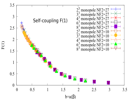
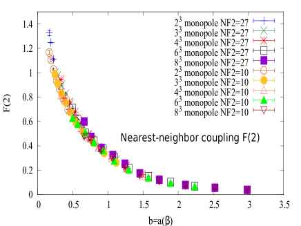
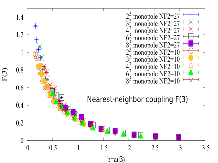
Figure 16: Comparison of the coupling constants of the self and two nearest-neighbor interactions between the actions composed of 27 ($NF2=27$) and 10 ($NF2=10$) quadratic interactions alone. The data are taken on $48^{4}$ in MCG

Figure 17: Comparison of the coupling constants of the two next nearest-neighbor interactions between the actions composed of 27 ($NF2=27$) and 10 ($NF2=10$) quadratic interactions alone.

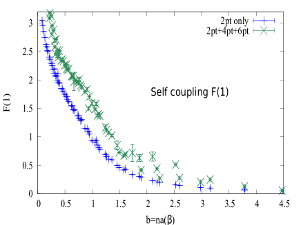
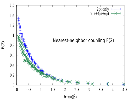
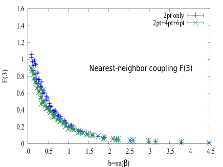
Figure 18: Comarison of the coupling constants of the self and two nearest-neighbor interactions versus $b=na(\beta)$ between the actions of $10$ two-point interactions with and without higher interactions on $48^{4}$ in MCG

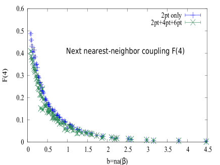
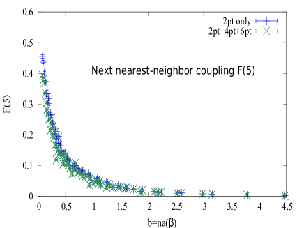
Figure 19: Comparison of the coupling constants of two next to nearest-neighbor interactions versus $b=na(\beta)$ between the actions of $10$ two-point interactions with and without higher interactions on $48^{4}$ in MCG

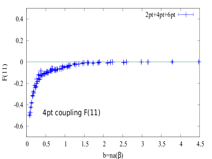
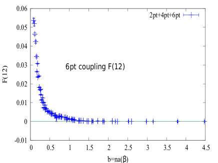
Figure 20: The coupling constants of four- and six-point interactions versus $b=na(\beta)$ in the action of $10$ two-point interactions with higher interactions on $48^{4}$ in MCG

Appendix B The form of the effective monopole action

As the form of the effective monopole action, we assume that only local and short-ranged interactions are dominant.

The quadratic interactions for each color $a$ used for the modified Swendsen method are shown in Table 3. Only the partner of the current multiplied by $k_{\mu}^{a}(s)$ are listed. All terms in which the relation of the two currents is equivalent should be added to satisfy translation and rotation invariances.

To check the dominance of quadratic interactions, we include the following four-point and six-point interactions among monopoles of the same color component listed in Table 4. The six-point interaction is included, since the coefficient of the four-point interaction is found to be negative numerically.

In the case of four and six-point interactions, there may exist color-mixing interactions via interactions with the gauge fields. We discuss the following color-mixed interactions as a simple example:

$$S^{(4)}_{dc}(k) = \sum_{s}\left(\sum_{\mu=-4}^{4}\sum_{a\neq b}(k_{\mu}^{a}(s))^{2}(k_{\mu}^{b}(s))^{2}\right)$$

$$S^{(6)}_{dc}(k) = \sum_{s}\left(\sum_{\mu=-4}^{4}(k_{\mu}^{1}(s))^{2}\sum_{\mu=-4}^{4}(k_{\mu}^{2}(s))^{2}\sum_{\mu=-4}^{4}(k_{\mu}^{3}(s))^{2}\right)$$

Appendix C Comparison of the effective monopole actions from numerical analyses

Various combinations of monopole interactions are tested numerically.

1. Color mixing effects are checked first by adopting

   $$S = \sum_{i=1}^{10}F(i)S^{(2)}_{i}(k)+F(11)S^{(4)}(k)+F(12)S^{(4)}_{dc}(k)$$

   $$+F(13)S^{(6)}(k)+F(14)S^{(6)}_{dc}(k),$$

   where the first $10$ quadratic interactions $S^{(2)}(k)$ alone in Table 3 are used for simplicity.

   As a whole, the convergence is rather difficult. When the convergence condition is relaxed, we get the convergent results for $n\geq 3$. An example is shown in Table 5 for $n=3$ and $\beta=3.3$. Since the coupling constants of the color-mixed interactions $F(12)$ and $F(14)$ are suppressed in comparison with those without no color mixing and stable convergence is not obtained for all cases, we did not consider any color mixing in the extensive studies done in this paper. The form of effective monopole action having no stable convergence is not a good choice for the application of the renormalization group study.

2. Under the condition of no color-mixing, we study four cases of effective monopole actions:
   (1) $27$ quadratic interactions in Table 3 plus higher interactions in Table 4.
   (2) First $10$ quadratic interactions with lattice distance $R\leq 2$ plus higher interactions in Table 4.
   (3) $27$ quadratic interactions in Table 3 alone.
   (4) First $10$ quadratic interactions with lattice distance $R\leq 2$ in Table 3 alone.
   An example for $\beta=3.2$ and $n=4$ blocking is shown in Table 6. The comparison can be done only for $n<8$ due to boundary effects, since the reduced lattice volume in $n=8$ is $6^{4}$ and $4^{4}$ in $n=12$ blocking. Similar behaviors are found for all $n<8$ and all $\beta$.

   • The coupling constants of four- and six-point interactions are very small, but they have non-negligible efffects on the most important quadratic self interaction $F(1)$ as seen from the data in the second and the fourth rows in Table 6. Big effects are not seen for other couplings up to $F(21)$.

   • The coupling constant $F(28)$ of the four-point interaction is negative, whereas that of the six-point interaction $F(29)$ is positive. This is similar to the results observed previously in MA gauge Chernodub:2000ax .

   • The first and the second rows in Table 6 show the comparison of both quadratic actions in (3) and (4). The most important self and the nearest-neighbor interactions are much the same. The couplings of the first $5$ quadratic interactions are compared in Fig.16 and Fig.17.

   • The differences of the cases (2) and (4) with and without higher interactions are shown in Fig.18 and Fig.19. All data satisfy the scaling but the differences are not negligible especially in the self coupling case. The coupling constants of higher interactions in the case (2) are plotted in Fig.20. Also scaling is seen beautifully.

   • In the main part of this paper, we focus on the most simple case (4), i.e., the action composed of first $10$ quadratic interactions alone, since then even $n=12$ could be studied in the renormalization group flow and the comparison between numerical data and analytic results from the blocking from the continuum is easy. Namely we will study the projection on to the coupling constant plane composed of the quadratic $10$ interactions of the renormalized action.

Appendix D Evaluation of the self-coupling term $D_{ii}^{-1}(0)$

The 10 quadratic interactions of $D_{\mu\nu}(s,s^{\prime})$ are explicitly written from Table 3 for each color component as

$$D_{\mu\nu}(s,s^{\prime}) = \sum_{i}F(i)(S_{i})_{\mu\nu}(s,s^{\prime}),$$ (62)

where $F(i)$ are coupling constants and the operators $S_{i}$ are shown as follows:

$$S_{1} = \delta_{s^{\prime},s}\delta_{\mu,\nu}$$

$$S_{2} = \frac{1}{2}\left[\delta_{s^{\prime},s+\mu}+\delta_{s^{\prime},s-\mu}\right]\delta_{\mu,\nu}$$

$$S_{3} = \frac{1}{2}\sum_{\alpha(\neq\mu)}\left[\delta_{s^{\prime},s+\alpha}+\delta_{s^{\prime},s-\alpha}\right]\delta_{\mu,\nu}$$

$$S_{4} = \frac{1}{4}\sum_{\alpha(\neq\mu)}[\delta_{s^{\prime},s+\mu+\alpha}+\delta_{s^{\prime},s+\mu-\alpha}$$

$$+\delta_{s^{\prime},s-\mu+\alpha}+\delta_{s^{\prime},s-\mu-\alpha}]\delta_{\mu,\nu}$$

$$S_{5} = \frac{1}{4}\sum_{\alpha\neq\beta(\neq\mu)}[\delta_{s^{\prime},s+\alpha+\beta}+\delta_{s^{\prime},s+\alpha-\beta}$$

$$+\delta_{s^{\prime},s-\alpha+\beta}+\delta_{s^{\prime},s-\alpha-\beta}]\delta_{\mu,\nu}$$

$$S_{8} = \frac{1}{2}\left[\delta_{s^{\prime},s+2\mu}+\delta_{s^{\prime},s-2\mu}\right]\delta_{\mu,\nu}$$

$$S_{10} = \frac{1}{2}\sum_{\alpha(\neq\mu)}\left[\delta_{s^{\prime},s+2\alpha}+\delta_{s^{\prime},s-2\alpha}\right]\delta_{\mu,\nu}.$$

Here irrelevant terms $S_{6},S_{7},S_{9}$ are not written explicitly. As shown in Table 6, the self-coupling $F(1)$ is much larger than other coupling constants. Hence the inverse propagator $D_{\mu\nu}^{-1}(s,s^{\prime})$ can be evaluated by the expansion with respect to $F(1)$. It is easy to see the self-coupling term contribution to the inverse proprgator comes only from the quadratic terms of $S_{i}$ in the expansion. Considering the numerical data showing $F(1)\gg F(2)\sim F(3)\gg F(4)\sim F(5)\gg\textrm{higher terms}$, the relevent non-negligible operators are $S_{2}^{2},\ S_{3}^{2},\ S_{4}^{2},\ S_{5}^{2},\ S_{2}^{4},\ S_{2}^{2}S_{3}^{2},\ S_{3}^{4}$. These operators are evaluated explicitly as

$$S_{2}^{2} = \frac{1}{2}S_{1}+\frac{1}{2}S_{8},$$

$$S_{3}^{2} = \frac{3}{2}S_{1}+S_{8}+\frac{1}{2}S_{10},$$

$$S_{4}^{2} = \frac{3}{4}S_{1}+\frac{1}{2}S_{5}+\frac{3}{4}S_{8}+\ldots,$$

$$S_{5}^{2} = \frac{3}{4}S_{1}+\frac{3}{4}S_{10}+\ldots,$$

$$\ S_{2}^{4} = \frac{3}{8}S_{1}+\ldots$$

$$S_{2}^{2}S_{3}^{2} = \frac{3}{4}S_{1}+\ldots,$$

$$S_{3}^{4} = \frac{25}{8}S_{1}+\ldots.$$

Hence we get

$$D_{ii}^{-1}(0) = \frac{1}{F(1)}+\frac{F(2)^{2}}{2F(1)^{3}}+\frac{3F(3)^{2}}{2F(1)^{3}}+\frac{3F(4)^{2}}{4F(1)^{3}}$$ (63)

$$+ \frac{3F(5)^{2}}{4F(1)^{3}}+\frac{3F(2)^{4}}{8F(1)^{5}}+\frac{9F(2)^{2}F(3)^{2}}{2F(1)^{5}}$$

$$+ \frac{25F(3)^{4}}{8F(1)^{5}}+\ldots.$$

References

- (1) Tsuneo Suzuki, A new scheme for color confinement due to violation of the non-Abelian Bianchi identities, hep-lat: arXiv:1402.1294 (2014)
- (2) Tsuneo Suzuki, Katsuya Ishiguro and Vitaly Bornyakov, A new scheme for color confinement and violation of the non-Abelian Bianchi identities(VNABI), hep-lat: arXiv:1712.05941 (2017)
- (3) T. A. DeGrand and D. Toussaint, Phys. Rev. D22, 2478 (1980).
- (4) T. Suzuki, M. Hasegawa, K. Ishiguro, Y. Koma and T. Sekido, Phys. Rev. D80, 054504 (2009).
- (5) T.L. Ivanenko, A. V. Pochinsky and M.I. Polikarpov, Phys. Lett. B302, 458 (1993). ”,
- (6) H. Shiba and T. Suzuki, Phys. Lett. B351, 519 (1995).
- (7) S. Kato, N. Nakamura, T. Suzuki and S. Kitahara, Nucl. Phys.B520,323 (1998).
- (8) M.N.Chernodub et al., Phys. Rev. D62 094506 (2000) and references therein.
- (9) L. Del Debbio, M. Faber, J. Greensite and S. Olejnik, Phys. Rev. D55, 2298 (1997)
- (10) L. Del Debbio, M. Faber, J. Giedt, J. Greensite and S. Olejnik, Phys. Rev. D58, 094501 (1998)
- (11) W. Bietenholz and U.J. Wiese Nucl. Phys. B464, 319 (1996); Phys. Lett. B 378, 222 (1996); W. Bietenholz, Int. J. Mod. Phys. A 15, 3341 (2000)
- (12) Biagio Lucini, Michael Teper and Urs Wenger,JHEP 0406,012 (2004)
- (13) M. G. Alford, W. Dimm, G. P. Lepage, G. Hockney, and P. B. Mackenzie, Phys. Lett. B 361, 87 (1995).
- (14) V. G. Bornyakov, D. A. Komarov and M.I. Polikarpov, Phys. Lett. B497, 151 (2001).
- (15) M. Faber, J. Greensite and S. Olejnik, JHEP 111, 053 (2001).
- (16) A. S. Kronfeld, M. L. Laursen, G. Schierholz, and U. J. Wiese, Phys. Lett. B198, 516 (1987).
- (17) A. S. Kronfeld, G. Schierholz, and U. J. Wiese, Nucl. Phys. B293, 461 (1987).
- (18) G. S. Bali, V. Bornyakov, M. Muller-Preussker and K. Schilling, Phys. Rev. D54, 2863 (1996).
- (19) R.H. Swendsen,Phys. Rev. Lett. 52,1165 (1984);
- (20) V. G. Bornyakov, E. -M. Ilgenfritz, and M. Muller-Preussker, Phys. Rev. D72, 054511 (2005).
- (21) G. I. Poulis, Phys. Rev. D 56, 161 (1997).
- (22) A. Hasenfratz and F. Knechtli, Phys. Rev. D 64, 034504 (2001).
- (23) A. Hasenfratz, R. Hoffmann and F. Knechtli, Nucl. Phys. Proc. Suppl. 106, 418 (2002).
- (24) C. Gattringer, R. Hoffmann and S. Schaefer, Phys. Rev. D 65, 094503 (2002).
- (25) V. G. Bornyakov et al. [DIK Collaboration], Phys. Rev. D 71, 114504 (2005).
- (26) M. Albanese et al. [APE Collaboration], Phys. Lett. B 192, 163 (1987).
- (27) T. Suzuki et al., Nucl. Phys. Proc. Suppl. 53, 531 (1997).
- (28) S. Fujimoto, S. Kato and T. Suzuki, Phys. Lett. B476, 437 (2000).
- (29) M.I.Polikarpov et al, Phys.Lett.B309, 133 (1993).
- (30) M.N. Chernodub, S. Kato, N. Nakamura, M.I. Polikarpov and T. Suzuki, hep-lat/9902013 (1999).
- (31) T. Suzuki, Prog.Theor.Phys. 80 (1988) 929; 81 (1989) 752; S. Maedan and T. Suzuki, Prog.Theor.Phys. 80 (1988) 929; S. Maedan , Prog.Theor.Phys. 84 (1990) 130.
- (32) I. Montvay and G. Münster, “Quantum Fields on a Lattice” Cambridge University Press.