Local-global model reduction method for stochastic optimal control problems constrained by partial differential equations

ABSTRACT

In this paper, a local-global model reduction method is presented to solve stochastic optimal control problems governed by partial differential equations (PDEs). If the optimal control problems involve uncertainty, we need to use a few random variables to parameterize the uncertainty. The stochastic optimal control problems require solving coupled optimality system for a large number of samples in the stochastic space to quantify the statistics of the system response and explore the uncertainty quantification. Thus the computation is prohibitively expensive. To overcome the difficulty, model reduction is necessary to significantly reduce the computation complexity. We exploit the advantages from both reduced basis method and Generalized Multiscale Finite Element Method (GMsFEM) and develop the local-global model reduction method for stochastic optimal control problems with PDE constraints. This local-global model reduction can achieve much more computation efficiency than using only local model reduction approach and only global model reduction approach. We recast the stochastic optimal problems in the framework of saddle-point problems and analyze the existence and uniqueness of the optimal solutions of the reduced model. In the local-global approach, most of computation steps are independent of each other. This is very desirable for scientific computation. Moreover, the online computation for each random sample is very fast via the proposed model reduction method. This allows us to compute the optimality system for a large number of samples. To demonstrate the performance of the local-global model reduction method, a few numerical examples are provided for different stochastic optimal control problems.

keywords: stochastic optimal control problem, reduced basis method, generalized multiscale finite element method, local-global model reduction

1 Introduction

Optimal control problems are often constrained with partial differential equations (PDEs) when modeling physical processes in sciences and engineering. For problems that involve uncertainty, stochastic information needs to be incorporated into the control problems. This leads to stochastic optimal control problems. To characterize the uncertainty, we often use random variables to parameterize the stochastic functions. In practical applications, uncertainties may arise from various sources such as the PDE coefficients, boundary conditions, external loadings and shape of physical domain. The uncertainty may have significant impact on the optimal solution. For deterministic optimal control problems, mathematical theories and computational methods have been developed and investigated for many years (see, e.g. [20, 32, 40]), while the development of stochastic optimal control problem governed by stochastic PDE have gained substantial attention from the last decades [12, 23, 24, 31, 42].

In this paper, we consider the stochastic optimal control problems with quadratic cost functional constrained by stochastic PDEs. For PDE-constrained optimization problems, there is a choice of whether to discretize-then-optimize or optimize-then-discretize, and there are different opinions regarding which route to take (see, e.g. [11, 37] for more discussion). We choose to optimize-discretize-then-reduce approach in this work. Existence and uniqueness of an optimal solution to stochastic optimal control problems was studied in [8, 24, 31, 35] in the framework of traditional FE method. It is known that the numerical solution of PDE-constrained optimization problems is computationally expensive because it requires the solutions of a system of PDEs arising from the optimality conditions: the state problem, the adjoint problem and a set of equations ensuring the optimality of the solution. Especially in the many-query context for parameterized PDEs, this computation becomes much more challenging and may lead to the “curse-of-dimensionality” in high dimensional stochastic spaces, which makes numerical computation very extensive.

There exist some efficient methods to solve the stochastic optimal control problems. The Monte Carlo method is one of the most straightforward schemes to get the approximate optimal solution in the stochastic space. However, it is to be blamed for its low convergence rate, thus leading to heavy computational cost when a full deterministic optimal control problem has to be solved for every sample. Stochastic Galerkin method has been proved to converge exponentially fast for smooth problems [5, 24]. Unfortunately, the tensor-product projection scheme produces a large-scale tensor system to be solved, bringing further computational difficulties. The works [12, 30, 42] made use of the stochastic collocation method, which can avoid the tensor-product large algebraic system encountered by the stochastic Galerkin method. However, when the optimality system is in high dimensional stochastic spaces, these techniques are needed to solve the optimality system for many times corresponding to the collocation nodes. To overcome these issues, model order reduction methods are necessary to solve large-scale stochastic optimal control problems in high dimensional stochastic spaces. Roughly speaking, there exist two categories for model order reduction. One is global model order reduction such as proper orthogonal decomposition and reduce basis (RB) method [22]. The other is local model order reduction such as coarsen finite element methods and sparse basis methods [25, 29]. The global model reduction method involves solving a few global problems. The local model reduction method may still have a large number of degree of freedoms and depend on the random parameters. To exploit the advantages from both local model reduction and global model reduction, we present a local-global model reduction approach to solve the stochastic optimal control problems in the paper. The local-global model reduction using POD and GMsFEM has been used in flows in heterogeneous porous media [1]. Our local-global model reduction here is based on reduced basis method and GMsFEM to solve stochastic optimal control problems.

Inspired by [36], we leverage inexpensive low-fidelity models to provide important information abut the high-fidelity model outputs and substantially reduce computation complexity. We build a low-fidelity model based on a RB method. RB method is one of global model order reduction methods and it allows to recast a computational demanding problem (“truth” problem) into a the reduced problem [10, 14, 21, 38, 41] with fast and reliable low-dimensional formulation. The main features of RB method [38, 41] are: (i) a posterior bound error estimation for choosing some optimal parameters; (ii) a fast convergent global approximation onto snapshot spaces; (iii) an offline-online procedure, yielding the RB functions in the offline stage and obtaining the online calculation for each new input parameter with inexpensive cost.

For the RB method, we can use FE method in a fine grid to get the accurate snapshot functions. For the computation of snapshot functions in large-scale or multiscale models, the number of degree of freedoms may be very large to resolve all scales in fine grid. Thus, the computation for snapshots may be very expensive. So it is desirable to develop an inexpensive low-fidelity model to obtain the snapshot functions. As a local model reduction method, Multiscale finite element method (MsFEM) [25, 27] is an efficient method to achieve a good trade-off between accuracy and efficiency. The main idea is to divide the fine scale problem into many local problems and use the solutions of the local problems to form a coarse scale model [27]. MsFEM incorporates the small-scale information to multiscale basis functions and capture the impact of small-scale features on the coarse-scale through a variational formulation. One of the most important features for MsFEM is that the multisacle basis functions can be computed in the offline stage and used repeatedly for the model with different source terms, boundary conditions and the coefficients with similar multiscale structures [19]. To capture complex heterogeneities and continuum scales in the models, one may need to use multiple basis functions per coarse block. To this end, Generalized Multiscale Finite Element Method (GMsFEM) [17, 18] have been developed in the framework of generalized finite element method [2, 34]. This approach extends MsFEM and constructs multiscale basis functions in each coarse element via local spectral problem. In each coarse element, the number of multiscale basis functions is much less than the number of fine-scale basis functions.

It is crucial to select the parameter samples with an optimal strategy when applying reduce basis method to solve stochastic optimal control problems. We will adopt the greedy algorithm [33] to choose optimal samples for snapshots in this paper. We can also use other methods to construct snapshots such as proper orthogonal decomposition and cross-validation [28]. In Fig. 1.1, we describe the schema to get the reduced order model using the proposed local-global model reduction method.

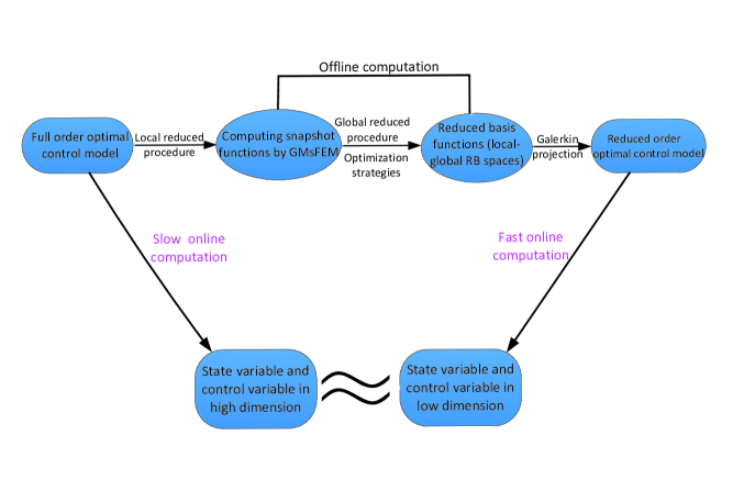
Figure 1.1: Schema of local-global model reduction for stochastic optimal control problems

The paper is structured as follows. In Section 2, we present some preliminaries and notations, the stochastic optimal control problems, and the global existence and uniqueness of optimal solutions. In Section 3, FE approximation for the optimal control problems is discussed. Section 4 is to present the construction of the global RB method and the equivalent reduced saddle point system and the local model reduction method via GMsFEM. In section 5, we address the local-global model reduction method and greedy sampling method used for constructing the optimal RB functions. In Section 6, we present a few numerical examples for different stochastic optimal control problems to illustrate the local-global model reduction method. Finally, some conclusions and comments are outlined in the last section.

2 Stochastic optimal control problems

In this subsection, we first introduce some notations used for the rest of paper and then present the stochastic optimal control problems. Then, we will recast the original optimal control problems into the framework of the saddle-point problem and consider the well-posedeness of the saddle-point system.

2.1 Preliminaries and notations

Let $(\mathcal{D},\mathcal{F},\mathcal{P})$ be a complete probability space. Here $\mathcal{D}$ is a set of outcomes $\omega\in\mathcal{D}$, $\mathcal{F}\subset 2^{\mathcal{D}}$ is the $\sigma$-algebra of events, and $\mathcal{P}:\mathcal{F}\rightarrow[0,1]$ is a probability measure. We assume that $\Omega$ is a convex bounded polygonal domain in $\mathbb{R}^{d}~{}(d\geq 1)$ with Lipschitz continuous boundary $\partial\Omega$. Let $v:\Omega\times\mathcal{D}\rightarrow\mathbb{R}$ represent a real-valued random field, i.e., real-valued random function defined in $\mathcal{D}$. For computation, the random field is usually approximated using a prescribed a finite number of random variables, $\mu(\omega)=\{\mu_{1},\mu_{2},\cdots,\mu_{m}\}$, i.e., $\mu(\cdot):\mathcal{D}\rightarrow\Gamma\subset\mathbb{R}^{m}~{}(m\geq 1)$. Thus, we use the random vector $\mu(\omega)$ to characterize the stochastic property of the random field. Let $\rho$ be the joint probability density function of $\mu(\omega)$.

We define the following tensor-product Hilbert space

$$\begin{split}H^{s}(\Omega)\otimes L^{2}_{\rho}(\Gamma):=\bigg{\{}v:\Omega\times\Gamma\rightarrow\mathbb{R}|v(\cdot,\mu)\in H^{s}(\Omega)~{}\text{and}~{}\|v(\cdot,\mu)\|_{H^{s}(\Omega)}\in L^{2}_{\rho}(\Gamma),\forall\mu\in\Gamma\bigg{\}}.\end{split}$$

We denote $\mathscr{H}^{s}(\Omega):=H^{s}(\Omega)\otimes L^{2}_{\rho}(\Gamma)$ to shorten the notation, and equip it with the following norm

$$\|v\|_{\mathscr{H}^{s}(\Omega)}:=\bigg{(}\int_{\Gamma}\|v(\cdot,\mu)\|^{2}_{H^{s}(\Omega)}\rho d\mu\bigg{)}^{1/2}.$$

In particular, $\mathscr{H}^{s}_{0}(\Omega)=\{v\in\mathscr{H}^{s}(\Omega):v|_{\partial\Omega}=0\}$. When $s=0$, we employ the abbreviated notion $\mathscr{L}^{2}(\Omega)$ to denote $\mathscr{H}^{0}(\Omega)$ by convention.

2.2 Problem definition

For a stochastic optimal control problem, the aim is to choose the control function $f(x,\mu(\omega))$ in such a way that the corresponding state function $u(x,\mu(\omega))$ is the best possible approximation to a desired state function $\hat{u}(x,\mu(\omega))$. The stochastic optimal control problem leads to minimizing an objective functional with some constraints. In the paper, we focus on the following optimal control problem

$$\min\limits_{\begin{subarray}{c}u\in\mathscr{H}^{1}(\Omega)\\ f\in\mathscr{L}^{2}(\Omega)\end{subarray}}J(u,f)=\frac{1}{2}\|u(x,\mu(\omega))-\hat{u}(x,\mu(\omega))\|^{2}_{\mathscr{L}^{2}(\Omega)}+\beta\|f(x,\mu(\omega))\|^{2}_{\mathscr{L}^{2}(\Omega)}$$ (2.1)

constrained by a stochastic PDE with the weak formulation

$$a(u,v;\mu(\omega))=(f,v;\mu(\omega))~{}~{}\forall v\in\mathscr{H}^{1}_{0}(\Omega),$$ (2.2)

subject to the Dirichlet boundary condition $u|_{\partial\Omega}=g(x)$. Here $J(u,f):\Omega\times\mathcal{D}\rightarrow\mathbb{R}$ is a cost-functional and $\beta$ is a positive constant. In the model problem, we assume that the state $u(x,\mu(\omega))$ and the control $f(x,\mu(\omega))$ are random fields represented by the random vector $\mu$.

The second term in (2.1) has a regularizing effect and is called a Tikhonov regularization. The $\beta$ is called a regularization parameter, which counteracts the tendency of the control to become locally unbounded and the cost functional $J(u,f)$ to approach its minimum. For the existence and uniqueness of the solution of the constraint (2.2), we assume that the bilinear form $a(\cdot,\cdot;\mu)$ is coercive and bounded over $H^{1}(\Omega)$ for any $\mu\in\Gamma$, i.e., there exist constants $\tilde{\alpha}_{0},\tilde{\alpha}_{1}>0$ such that

$$\tilde{\alpha}(\mu)=\inf\limits_{v\in H^{1}(\Omega)}\frac{a(v,v;\mu)}{\|v\|^{2}_{H^{1}(\Omega)}}\geq\tilde{\alpha}_{0},\quad\forall\mu\in\Gamma,$$

and

$$a(u,v;\mu)\leq\tilde{\alpha}_{1}\|u\|_{H^{1}(\Omega)}\|v\|_{H^{1}(\Omega)},\quad\forall\mu\in\Gamma,$$

for all $u,v\in H^{1}(\Omega)$.

2.3 Saddle-point formulation for optimal control problem

In this subsection we introduce the variational formulation of the distributed stochastic optimal control problem. We apply Lagrangian approach [43] for the derivation of the stochastic optimality system for the optimal control problem (2.1-2.2). We define the following stochastic Lagrangian functional as

$$\mathcal{L}(u,f,\lambda)=J(u,f)+a(u,\lambda;\mu)-(f,\lambda;\mu),$$ (2.3)

where $\lambda\in\mathscr{H}^{1}_{0}(\Omega)$ is the Lagrangian parameter or adjoint variable. By taking the Fr$\acute{e}$chet derivative of the Lagrangian functional (2.3) with respect to the variables $u,f,\lambda$ and evaluating at $\tilde{u},\tilde{f},\tilde{\lambda}$, we can get the first order necessary optimality conditions [12, 13] of stochastic control problem (2.1-2.2), i.e.,

$$\begin{cases}\begin{split}a(u,\widetilde{u};\mu)&=(f,\widetilde{u};\mu)~{}\forall\widetilde{u}\in\mathscr{H}^{1}_{0}(\Omega)~{}~{}(\text{state equation}),\\ a^{\prime}(\lambda,\widetilde{\lambda};\mu)&=-(u-\hat{u},\widetilde{\lambda};\mu)~{}\forall\widetilde{\lambda}\in\mathscr{H}^{1}_{0}(\Omega)~{}~{}(\text{adjoint equation}),\\ 2\beta(f,\widetilde{f};\mu)&=(\widetilde{f},\lambda;\mu)~{}\forall\widetilde{f}\in\mathscr{L}^{2}(\Omega)~{}~{}(\text{gradient equation}),\end{split}\end{cases}$$ (2.4)

where $a^{\prime}(\lambda,\widetilde{\lambda};\mu)=a(\widetilde{\lambda},\lambda;\mu)$ is the adjoint bilinear form, and $(\cdot,\cdot;\mu)$ represents the general $L^{2}$ inner product.

As shown in [23, 24, 42], the optimality system (2.4) only has local optimal solutions. To demonstrate the global existence and uniqueness of the optimal solution, we will derive a stochastic saddle point formulation of the optimal control problem (2.1-2.2).

First of all, we introduce the new variables $\underline{u}=(u,f)\in\mathscr{U}$ and $\underline{v}=(v,h)\in\mathscr{U}$, where the tensor space $\mathscr{U}=\mathscr{H}^{1}(\Omega)\times\mathscr{L}^{2}(\Omega)$ is equipped with graph norm $\|\underline{u}\|_{\mathscr{U}}=\|u\|_{\mathscr{H}^{1}(\Omega)}+\|f\|_{\mathscr{L}^{2}(\Omega)}$. We define the bilinear forms $\mathcal{A}(\cdot,\cdot):\mathscr{U}\times\mathscr{U}\rightarrow\mathbb{R}$ and $\mathcal{B}(\cdot,\cdot):\mathscr{U}\times\mathscr{H}^{1}_{0}(\Omega)\rightarrow\mathbb{R}$ by

$$\begin{cases}\begin{split}\mathcal{A}(\underline{u},\underline{v})&:=(u,v)+2\beta(f,h;\mu),\\ \mathcal{B}(\underline{u},q)&:=a(u,q;\mu)-(f,q;\mu),\\ \end{split}\end{cases}$$ (2.5)

respectively. With the new definitions, we have the following minimization problem equivalent to the original optimal problem (2.1-2.2), that is

$$\begin{cases}\begin{split}\min\limits_{\underline{u}\in\mathscr{U}_{ad}}\mathcal{J}(\underline{u})&=\frac{1}{2}\mathcal{A}(\underline{u},\underline{u})-(\underline{\hat{u}},\underline{u}),\\ s.t.~{}~{}\mathcal{B}(\underline{u},\widetilde{u})&=(g,\widetilde{u})_{\partial\Omega}\quad\forall\widetilde{u}\in\mathscr{H}^{1}_{0}(\Omega),\end{split}\end{cases}$$ (2.6)

where $\underline{\hat{u}}=(\hat{u},0)$, $(\underline{\hat{u}},\underline{u})=(\hat{u},u)$ and $\mathscr{U}_{ad}\subset\mathscr{U}$ is the admissible set. Moreover, the equivalent saddle point problem for (2.6) is to find: $(\underline{u},\lambda)\in\mathscr{U}\times\mathscr{H}^{1}(\Omega)$ such that

$$\begin{cases}\begin{split}\mathcal{A}(\underline{u},\underline{v})+\mathcal{B}(\underline{v},\lambda)&=(\underline{\hat{u}},\underline{v})\quad\forall\underline{v}\in\mathscr{U},\\ \mathcal{B}(\underline{u},\widetilde{u})&=(g,\widetilde{u})_{\partial\Omega}\quad\forall\widetilde{u}\in\mathscr{H}^{1}_{0}(\Omega).\end{split}\end{cases}$$ (2.7)

Lemma 2.1.

Let $\mathscr{U}_{0}:=\{\underline{u}\in\mathscr{U}:\mathcal{B}(\underline{u},\widetilde{u})=0~{}~{}\forall\widetilde{u}\in\mathscr{H}^{1}_{0}(\Omega)\}$ be the kernel space of bilinear form $\mathcal{B}(\cdot,\cdot)$. Then the minimization problem (2.6) is equivalent to the saddle point formulation (2.7). Furthermore, the original minimization (2.1-2.2) and (2.4) is also equivalent.

Proof.

To prove the equivalence, we need to verify the continuity and coercivity properties of $\mathcal{A}(\cdot,\cdot)$ and the inf-sup condition for $\mathcal{B}(\cdot,\cdot)$ [7, 9]. By the definition of bilinear form $\mathcal{A}(\cdot,\cdot)$ in (2.5), we have $\mathcal{A}(\underline{u},\underline{v})=\mathcal{A}(\underline{v},\underline{u})$ and $\mathcal{A}(\underline{u},\underline{u})\geq 0$. So $\mathcal{A}$ is symmetric and nonnegative. Because

$$\begin{split}\mathcal{A}(\underline{u},\underline{v})&\leq\|u\|_{\mathscr{L}^{2}(\Omega)}\|v\|_{\mathscr{L}^{2}(\Omega)}+\gamma\|f\|_{\mathscr{L}^{2}(\Omega)}\|h\|_{\mathscr{L}^{2}(\Omega)}\\ &\leq\|u\|_{\mathscr{H}^{1}(\Omega)}\|v\|_{\mathscr{H}^{1}(\Omega)}+\gamma\|f\|_{\mathscr{L}^{2}(\Omega)}\|h\|_{\mathscr{L}^{2}(\Omega)}\\ &\leq\gamma_{a}\|\underline{u}\|_{\mathscr{U}}\|\underline{v}\|_{\mathscr{U}},\end{split}$$

$\mathcal{A}(\cdot,\cdot)$ is continuous on $\mathscr{U}\times\mathscr{U}$ and $\gamma_{a}$ is a constant depending on $\gamma$. By the definition of kernel space $\mathscr{U}_{0}$, we have $\mathcal{B}(\underline{u},\widetilde{u})=0$, that is $a(u,\widetilde{u};\mu)=(f,\widetilde{u};\mu),~{}\forall\widetilde{u}\in\mathscr{H}^{1}_{0}(\Omega)$. Hence, by the coercivity property of $a(\cdot,\cdot;\mu)$ and Cauchy-Schwarz inequality, it holds that $\|u\|_{\mathscr{H}^{1}(\Omega)}\leq C_{1}\|f\|_{\mathscr{L}^{2}(\Omega)}$ with appropriate constant $C_{1}$. Then the coercivity of $\mathcal{A}(\cdot,\cdot)$ follows,

$$\begin{split}\mathcal{A}(\underline{u},\underline{u})&=\|u\|^{2}_{\mathscr{L}^{2}(\Omega)}+\beta\|f\|^{2}_{\mathscr{L}^{2}(\Omega)}\\ &\geq\|u\|^{2}_{\mathscr{L}^{2}(\Omega)}+\frac{\beta}{2C_{1}}\|u\|^{2}_{\mathscr{H}^{1}(\Omega)}+\frac{\beta}{2}\|f\|^{2}_{\mathscr{L}^{2}(\Omega)}\\ &\geq\gamma_{b}\|\underline{u}\|^{2}_{\mathscr{U}},\end{split}$$

where the coefficient $\gamma_{b}=\max\{\frac{\beta}{2C_{1}},\frac{\beta}{2}\}$.

Next, by the definition of $\mathcal{B}(\cdot,\cdot)$ and the continuity property of bilinear form $a(\cdot,\cdot;\mu)$, we have

$$\begin{split}\mathcal{B}(\underline{u},\widetilde{u})&\leq\tilde{\alpha}_{1}\|u\|_{\mathscr{H}^{1}(\Omega)}\|\widetilde{u}\|_{\mathscr{H}^{1}(\Omega)}+\|f\|_{\mathscr{L}^{2}(\Omega)}\|\widetilde{u}\|_{\mathscr{L}^{2}(\Omega)}\\ &\leq\max\{\tilde{\alpha}_{1},1\}\|\underline{u}\|_{\mathscr{U}}\|\widetilde{u}\|_{\mathscr{H}^{1}(\Omega)},\end{split}$$

where $\tilde{\alpha}_{1}$ is the continuity constant of the bilinear form $a(\cdot,\cdot;\mu)$.

Finally, we exploit the fact that state variable and adjoint variable belong to the same space $\mathscr{H}^{1}(\Omega)$ and the coercivity property of the bilinear form $a(\cdot,\cdot;\mu)$. The inf-sup condition of $\mathcal{B}(\cdot,\cdot)$ on $\mathscr{U}\times\mathscr{H}^{1}(\Omega)$ follows

$$\begin{split}\sup\limits_{0\neq\underline{u}\in\mathscr{U}}\frac{\mathcal{B}(\underline{u},\widetilde{u})}{\|\underline{u}\|_{\mathscr{U}}}&=\sup\limits_{0\neq(u,h)\in\mathscr{H}^{1}(\Omega)\times\mathscr{L}^{2}(\Omega)}\frac{a(u,\widetilde{u};\mu)-(h,\widetilde{u};\mu)}{\|u\|_{\mathscr{H}^{1}(\Omega)}+\|h\|_{\mathscr{L}^{2}(\Omega)}}\\ &\geq\sup\limits_{0\neq(u,0)\in\mathscr{H}^{1}(\Omega)\times\mathscr{L}^{2}(\Omega)}\frac{a(u,\widetilde{u};\mu)}{\|u\|_{\mathscr{H}^{1}(\Omega)}}\\ &\geq\tilde{\alpha}(\mu)\|\widetilde{u}\|_{\mathscr{H}^{1}(\Omega)}.\end{split}$$

Here $\tilde{\alpha}(\mu)$ is the infimum of the bilinear form $a(\cdot,\cdot;\mu)$.
∎

Lemma 2.2.

The saddle point problem (2.7) is equivalent to the stochastic optimality system (2.4).

Proof.

Equation (2.7) amounts to finding $(u,f,\lambda)\in\mathscr{H}^{1}(\Omega)\times\mathscr{L}^{2}(\Omega)\times\mathscr{H}^{1}_{0}(\Omega)$ such that

$$\begin{cases}\begin{split}(u,v)+2\beta(f,h;\mu)+a(v,\lambda;\mu)-(h,\lambda;\mu)&=(\hat{u},v)\quad\forall v\in\mathscr{H}^{1}(\Omega),~{}\forall h\in\mathscr{L}^{2}(\Omega)\\ a(u,\widetilde{u};\mu)-(f,\widetilde{u};\mu)&=(g,\widetilde{u})_{\partial\Omega}\quad\forall\widetilde{u}\in\mathscr{H}^{1}_{0}(\Omega).\end{split}\end{cases}$$ (2.8)

As we can see, $(\ref{full-optimal-system})_{2}$ coincides with the state equation in (2.4). Furthermore, we can obtain the adjoint equation of system (2.4) by taking $h=0$ in $(\ref{full-optimal-system})_{1}$. With $v=0$, we can recover the optimality conditions $(\ref{optimal-system1})_{3}$. Conversely, $(\ref{full-optimal-system})_{1}$ is retrieved by adding the adjoint equation and gradient equation in (2.4). ∎

Theorem 2.3.

Provided that assumptions in Lemma 2.1 are satisfied, we can obtain the global existence of a unique solution to the minimization problem (2.7). Furthermore, we have the following estimates:

$$\begin{split}\|\underline{u}\|_{\mathscr{U}}\leq\gamma_{1}\|\hat{u}\|_{\mathscr{L}^{2}(\Omega)}+\varrho_{1}\|g\|_{\mathscr{L}^{2}(\partial\Omega)},\\ \|\lambda\|_{\mathscr{U}}\leq\gamma_{2}\|\hat{u}\|_{\mathscr{L}^{2}(\Omega)}+\varrho_{2}\|g\|_{\mathscr{L}^{2}(\partial\Omega)},\\ \end{split}$$

where $\gamma_{1}$, $\gamma_{2}$, $\varrho_{1}$ and $\varrho_{2}$ are all positive constants.

Due to the above equivalence, it is sufficient to compute the solution of (2.7) or (2.4) to solve the original optimal control problem (2.1-2.2).

3 FE approximation for optimal control problem

Before giving the framework of FE approximation for stochastic optimal control problems, we will make an assumption that both the parametric bilinear form $a(\cdot,\cdot;\mu)$ and the parametric linear form $(f,\cdot;\mu)$ are affine with respect to $\mu$ , i.e.,

$$\begin{cases}\begin{split}a(u,v;\mu)&=\sum\limits^{Q_{a}}_{q=1}Q^{q}_{a}(\mu)a^{q}(u,v)\quad\forall u,v\in H^{1}(\Omega),~{}\forall\mu\in\Gamma,\\ (f,v;\mu)&=\sum\limits^{Q_{f}}_{q=1}Q^{q}_{f}(\mu)(f^{q},v)\quad\forall f^{q}\in L^{2}(\Omega),~{}v\in H^{1}(\Omega),~{}\forall\mu\in\Gamma.\\ \end{split}\end{cases}$$ (3.9)

In the above, for $q=1,\cdots,Q_{a}$, each $Q^{q}_{a}(\mu):\Gamma\rightarrow\mathbb{R}$ is a $\mu$-dependent function and $a^{q}(\cdot,\cdot):H^{1}(\Omega)\times H^{1}(\Omega)\rightarrow\mathbb{R}$ is a symmetric bilinear form independent of $\mu$. Similarly, $Q^{q}_{f}(\mu):\Gamma\rightarrow\mathbb{R},q=1,\cdots,Q_{f},$ are $\mu$-dependent functions and $(f^{q},\cdot):L^{2}(\Omega)\times H^{1}(\Omega)\rightarrow\mathbb{R},q=1,\cdots,Q_{f}$, are continuous functionals independent of $\mu$. The affine assumptions $(\ref{affine})$ will play a crucial computational role in the offline-online computational procedure. For the nonaffine parametric bilinear form $a(\cdot,\cdot;\mu)$ and parametric linear form $(f,\cdot;\mu)$, we can use the Empirical Interpolation Method (EIM), see, e.g. [6, 22, 38], to approximate them with an affine representation.

Let $\mathcal{T}_{h}$ be a uniform partition of the physical domain $\Omega$. Let $V^{h}(\Omega)\subset H^{1}(\Omega)$ be the FE space on the fine grid $\mathcal{T}_{h}$ and $V^{h}_{0}(\Omega)\subset V^{h}(\Omega)$ with vanish boundary values. We let $N_{h}$ be the number of vertices, $N_{e}$ be the number of elements in the fine mesh and the dimension of FE space be $\mathcal{N}$. Furthermore, we assume that $M_{h}(\Omega)$ is the finite dimensional subspace of $L^{2}(\Omega)$ and $\mathcal{M}_{h}(\Omega)$ is also the finite dimensional subspace of $\mathscr{L}^{2}(\Omega)$ with $\mathcal{M}_{h}(\Omega)=M_{h}(\Omega)\otimes L^{2}_{\rho}(\Gamma)$.

Given any $\mu\in\Gamma$, by applying Galerkin projection of $\mathscr{U}_{h}\otimes\mathscr{V}^{h}_{0}(\Omega)\subset\mathscr{U}\otimes\mathscr{H}^{1}_{0}(\Omega)$, where $\mathscr{U}_{h}:=\mathscr{V}^{h}_{0}(\Omega)\otimes\mathcal{M}_{h}(\Omega)$, we obtain FE formulation of the saddle point problem (2.7) as: $(\underline{u}_{h},\lambda_{h})\in\mathscr{U}_{h}\times\mathscr{V}^{h}_{0}(\Omega)$ such that

$$\begin{cases}\begin{split}\mathcal{A}(\underline{u}_{h},\underline{v}_{h})+\mathcal{B}(\underline{v}_{h},\lambda_{h})&=(\underline{\hat{u}},\underline{v}_{h})\quad\forall\underline{v}_{h}\in\mathscr{U}_{h},\\ \mathcal{B}(\underline{u}_{h},\widetilde{u}_{h})&=(g,\widetilde{u}_{h})_{\partial\Omega}\quad\forall\widetilde{u}_{h}\in\mathscr{V}^{h}_{0}(\Omega).\end{split}\end{cases}$$ (3.10)

Mimicking the proofs in subsection 2.3, we can easily show that $\mathcal{A}(\cdot,\cdot)$ is bounded and coercive. Moreover, the bilinear form $\mathcal{B}(\cdot,\cdot)$ satisfies inf-sup condition.

The Galerkin formulation of (3.10) is to find $(u_{h},f_{h},\lambda_{h})\in\mathscr{V}^{h}_{0}(\Omega)\otimes\mathcal{M}_{h}(\Omega)\otimes\mathscr{V}^{h}_{0}(\Omega)$ such that

$$\begin{cases}\begin{split}a(u_{h},\widetilde{u}_{h};\mu)&=(f_{h},\widetilde{u}_{h};\mu)\quad\forall\widetilde{u}_{h}\in\mathscr{V}^{h}_{0}(\Omega),\\ a(\lambda_{h},\widetilde{\lambda}_{h};\mu)&=-(u_{h}-\hat{u},\widetilde{\lambda}_{h};\mu)\quad\forall\widetilde{\lambda}_{h}\in\mathscr{V}^{h}_{0}(\Omega),\\ 2\beta(f_{h},\widetilde{f}_{h};\mu)&=(\widetilde{f}_{h},\lambda_{h};\mu)\quad\forall\widetilde{f}_{h}\in\mathcal{M}_{h}(\Omega),\end{split}\end{cases}$$ (3.11)

where $\mathscr{V}^{h}_{0}(\Omega):=V^{h}_{0}(\Omega)\otimes L^{2}_{\rho}(\Gamma)$. If the basis functions of spaces $\mathcal{M}_{h}(\Omega)$ and $V^{h}_{0}(\Omega)$ are denoted by $\{\phi_{k}\}^{N_{e}}_{k=1}$ and $\{\psi_{i}\}^{N_{h}}_{i=1}$, we can represent the variables in (3.11) with the linear combination of the corresponding basis functions as

$$u_{h}=\sum\limits^{N_{h}}_{i=1}u_{h,i}\psi_{i},\quad f_{h}=\sum\limits^{N_{e}}_{j=1}f_{h,j}\phi_{j},\quad\lambda_{h}=\sum\limits^{N_{h}}_{k=1}\lambda_{h,k}\psi_{k}.$$

Furthermore, if affine assumption (3.9) holds, the optimality system (3.11) will be

$$\begin{cases}\begin{split}&\sum\limits^{Q_{a}}_{q=1}\sum\limits^{N_{h}}_{i=1}Q^{q}_{a}(\mu)u_{h,i}(\mu)a^{q}(\psi_{i},\psi_{i^{\prime}})=\sum\limits^{N_{e}}_{j=1}f_{h,j}(\mu)(\phi_{j},\psi_{i^{\prime}}),\\ &\sum\limits^{Q_{a}}_{q^{\prime}=1}\sum\limits^{N_{h}}_{k=1}Q^{q^{\prime}}_{a}(\mu)\lambda_{h,k}(\mu)a^{q^{\prime}}(\psi_{k},\psi_{k^{\prime}})+\sum\limits^{N_{h}}_{i=1}u_{h,i}(\mu)(\psi_{i},\psi_{k^{\prime}})=-\sum\limits^{Q_{u}}_{p=1}\widehat{u}_{p}(\mu)(\overline{\hat{u}}_{p},\psi_{k^{\prime}}),\\ &2\beta\sum\limits^{N_{e}}_{j=1}\sum\limits^{N_{e}}_{j^{\prime}=1}f_{h,j}(\mu)f_{h,j^{\prime}}(\mu)(\phi_{j},\phi_{j^{\prime}})=\sum\limits^{N_{h}}_{k=1}\lambda_{h,k}(\mu)(\phi_{j^{\prime}},\psi_{k}).\end{split}\end{cases}$$

Then the algebraic formulation of (3.11) reads

$$\underbrace{\left[\begin{array}[]{ccc}2\beta M_{1,h}(\mu)&0&-M^{T}_{2,h}(\mu)\\ 0&M_{3,h}(\mu)&K^{T}_{h}(\mu)\\ -M_{2,h}(\mu)&K_{h}(\mu)&0\end{array}\right]}\limits_{\Lambda_{h}(\mu)\in\mathbb{R}^{(2N_{h}+N_{e})\times(2N_{h}+N_{e})}}\left[\begin{array}[]{c}F(\mu)\\ u(\mu)\\ \lambda(\mu)\end{array}\right]=\left[\begin{array}[]{c}0\\ \overline{\widehat{U}}\\ d\end{array}\right],$$ (3.12)

where

$$\begin{split}&(M_{1,h})_{j,j^{\prime}}=(\phi_{j},\phi_{j^{\prime}}),1\leq j,j^{\prime}\leq N_{e},\\ &(M_{2,h})_{k,j^{\prime}}=(\phi_{j^{\prime}},\psi_{k}),1\leq j^{\prime}\leq N_{e},1\leq k\leq N_{h},\\ &(M_{3,h})_{i,k^{\prime}}=(\psi_{i},\psi_{k^{\prime}}),(K^{q}_{h})_{k,k^{\prime}}=a^{q}(\psi_{k},\psi_{k^{\prime}}),1\leq i,k,k^{\prime}\leq N_{h},\\ &(\widehat{U}_{p})_{k^{\prime}}=(\overline{\hat{u}}_{p},\psi_{k^{\prime}}),1\leq k^{\prime}\leq N_{h},\\ &K_{h}=\sum^{Q_{a}}_{q=1}Q^{q}_{a}(\mu)K^{q}_{h},\overline{\widehat{U}}=\sum^{Q_{u}}_{p=1}\widehat{u}_{p}(\mu)\widehat{U}_{p}.\end{split}$$ (3.13)

Here $u(\mu)$, $F(\mu)$ and $\lambda(\mu)$ denote the vectors of the coefficients in the expansion of $u_{h}(\mu)$, $f_{h}(\mu)$, $\lambda_{h}(\mu)$, respectively. The term coming from the boundary values of $u_{h}$ is denoted by $d$. For simplicity of notation, we have suppressed the size of zero-blocks. In the following, we will change the size of zeros-blocks according to the size of the related nonzero-blocks.

With the affine assumption (3.9), stiffness-matrix and mass-matrices are performed only once at the offline stage with expensive computational cost. At the online stage, for each new parameter sample $\mu\in\Gamma$, all the coefficients $Q^{q}_{a}(\mu)$ and $\widehat{u}_{p}(\mu)$ are evaluated, and the $(2N_{h}+N_{e})\times(2N_{h}+N_{e})$ linear system (5.30) is assembled and solved. The online operation count is $O(Q_{a}\mathcal{N}^{2})+O(Q_{u}\mathcal{N})$ to perform the sum of the last line in (3.13), and is $O((3\mathcal{N})^{3})$ to invert the matrix $\Lambda_{h}(\mu)$. Thus, the total online operation count to get the FE optimal solutions for each sample $\mu$ is

$$O(Q_{a}\mathcal{N}^{2})+O(Q_{u}\mathcal{N})+O((3\mathcal{N})^{3}),$$

which depends on the dimension of FE space $\mathcal{N}$. We define the spaces for the state, control, and adjoint variable, respectively, as

$$\begin{cases}\begin{split}X^{\mathcal{N}}_{h}(\Omega)=\text{span}\{u_{h}(\mu),\forall\mu\in\Gamma\},\\ Y^{\mathcal{N}}_{h}(\Omega)=\text{span}\{f_{h}(\mu),\forall\mu\in\Gamma\},\\ Z^{\mathcal{N}}_{h}(\Omega)=\text{span}\{\lambda_{h}(\mu),\forall\mu\in\Gamma\}.\end{split}\end{cases}$$ (3.14)

4 The global reduced basis method and the local model reduction method

In Section 2.3 and Section 3, we can see that both the minimization problems and the equivalent optimality systems are related to the parameter sample $\mu$. This means that we need to compute the optimality system for one time with a given random sample. This is a many-query problem and the computational cost will be very expensive. To overcome the difficulty, we build a reduced model to improve computation efficiency. In this section, we introduce a local-global model reduction method to construct a low-fidelity optimal control model. When performing the optimal process for a new given configuration, the solution will be computed efficiently.

4.1 The global reduced basis approximation

In this section, we follow the framework [26, 28, 29, 39, 41] to present the global RB method for solving stochastic optimal control problems. The essential components of the RB method: RB projection and optimality system. An offline-online computational stratagem will be presented.

4.1.1 Construction of global reduced basis approximation spaces and Galerkin projection

We assume that we have been given FE approximation spaces $V^{h}(\Omega)$, $M_{h}(\Omega)$ in a fine grid with (typically very large) dimensions $\mathcal{N}$ and $N_{e}$. The spaces $\mathscr{V}_{h}(\Omega)$ and $\mathcal{M}_{h}(\Omega)$ are automatically given. Given a positive integer $N_{max}$, we then introduce an associated sequence of (what shall ultimately be reduced basis) approximation spaces: for $N=1,\cdots,N_{max}$, $X^{N}_{h}(\Omega)$ is an N-dimensional subspace of $X^{\mathcal{N}}_{h}(\Omega)$. Let $\{X^{n}_{h}\}^{N_{max}}_{n=1}$ be nested, that is, $X^{1}_{h}\subset X^{2}_{h}\subset\cdots\subset X^{N_{max}}_{h}\subset X^{\mathcal{N}}_{h}(\Omega)\subset\mathscr{V}^{h}(\Omega)$. For the control variable $f$, we also define the similar subspaces: $Y^{1}_{h}\subset Y^{2}_{h}\subset\cdots\subset Y^{N_{max}}_{h}\subset Y^{\mathcal{N}}_{h}(\Omega)\subset\mathcal{M}_{h}(\Omega)$. For the adjoint variable $\lambda$, the set of nested subspaces is: $Z^{1}_{h}\subset Z^{2}_{h}\subset\cdots\subset Z^{N_{max}}_{h}\subset Z^{\mathcal{N}}_{h}(\Omega)\subset\mathscr{V}^{h}(\Omega)$. These nested subspaces are crucial in ensuring (memory) efficiency of the resulting RB approximation.

In order to define a sequence of Lagrange spaces $\{X^{N}_{h}(\Omega),Y^{N}_{h}(\Omega),Z^{N}_{h}(\Omega),1\leq N\leq N_{max}\}$, we first use

$$S_{N}=\{\mu^{1},\cdots,\mu^{N},1\leq N\leq N_{max}\}$$

to denote the set of properly selected parameter samples from $\Gamma$. The associated Lagrange RB spaces are

$$\begin{split}\begin{cases}X^{N}_{h}(\Omega)=\text{span}\{u_{h}(\mu^{n}),1\leq n\leq N\},\\ Y^{N}_{h}(\Omega)=\text{span}\{f_{h}(\mu^{n}),1\leq n\leq N\},\\ Z^{N}_{h}(\Omega)=\text{span}\{\lambda_{h}(\mu^{n}),1\leq n\leq N\},\end{cases}\end{split}$$ (4.15)

and denote $\mathcal{U}^{N}_{h}(\Omega)=X^{N}_{h}(\Omega)\times Y^{N}_{h}(\Omega)$.

The $u_{h}(\mu^{n}),f_{h}(\mu^{n}),\lambda_{h}(\mu^{n})$, $1\leq n\leq N_{max}$, are often referred to as “snapshots” of the parametric manifolds and are obtained by solving (3.11) for $\mu^{n}$, $1\leq n\leq N_{max}$. The choice of the parameters $\{\mu^{n}\}^{N_{max}}_{n=1}$ will effect on the fidelity of the reduced model to approximate the original model. To choose the set of optimal parameter samples, we will use a sampling strategy, greedy algorithm, in Section 5.2.

By using Galerkin projection onto the low-dimensional subspace $\mathscr{U}^{N}_{h}(\Omega)\times Z^{N}_{h}(\Omega)$, the following RB approximation can be obtained: given $\mu\in\Gamma$, find $(\underline{u}^{N}_{g},\lambda^{N}_{g})\in\mathscr{U}^{N}_{h}(\Omega)\times Z^{N}_{h}(\Omega)$ such that

$$\begin{cases}\begin{split}\mathcal{A}(\underline{u}_{g},\underline{v}_{g})+\mathcal{B}(\underline{v}_{g},\lambda_{g})&=(\underline{\hat{u}},\underline{v}_{g})\quad\forall\underline{v}_{g}\in\mathscr{U}^{N}_{h},\\ \mathcal{B}(\underline{u}_{g},\widetilde{u}_{g})&=(g,\widetilde{u}_{g})_{\partial\Omega}\quad\forall\widetilde{u}_{g}\in Z^{N}_{h}(\Omega).\end{split}\end{cases}$$ (4.16)

Next, we discuss the well-posedness of the global RB approximation (4.16). The continuity of the bilinear forms is automatically inherited from the FE spaces. Similarly, with the kernel space of bilinear form $\mathcal{B}(\cdot,\cdot;\mu)$ as $\mathscr{U}^{N}_{0}:=\{\underline{u}_{g}\in\mathscr{U}^{N}_{h}:\mathcal{B}(\underline{u}_{g},\widetilde{u}_{g})=0~{}~{}\forall\widetilde{u}_{g}\in Z^{N}_{h}(\Omega)\}$, the coercivity of bilinear form $\mathcal{A}(\cdot,\cdot;\mu)$ can be guaranteed. In the continuous case (or approximated by FE method), both the state and adjoint spaces belong to $\mathscr{H}^{1}(\Omega)$ (or $\mathscr{V}^{h}(\Omega)$) and the bilinear form $\mathcal{B}(\cdot,\cdot;\mu)$ satisfies the inf-sup condition. But with the choice (4.15), we lose this property on the Lagrange RB spaces, i.e., $X^{N}_{h}(\Omega)\neq Z^{N}_{h}(\Omega)$.

In order to recovery the inf-sup condition for system (4.16), we therefore need to enrich in some way at least one of the RB spaces involved. With the method considered in some previous works [16, 35], we use an enriched RB space $Q^{N}_{h}(\Omega)$ as the union $X^{N}_{h}(\Omega)$ and $Z^{N}_{h}(\Omega)$, i.e.,

$$Q^{N}_{h}(\Omega)=X^{N}_{h}(\Omega)\cup Z^{N}_{h}(\Omega)=\text{span}\{u_{h}(\mu^{n}),\lambda_{h}(\mu^{n}),1\leq n\leq N\},$$ (4.17)

and we let

$$X^{N}_{h}(\Omega)=Q^{N}_{h}(\Omega),\quad\mathcal{U}^{N}_{h}(\Omega)=X^{N}_{h}(\Omega)\times Y^{N}_{h}(\Omega),\quad Z^{N}_{h}(\Omega)=Q^{N}_{h}(\Omega).$$ (4.18)

Lemma 4.1.

With the definition of reduced spaces $\mathcal{U}^{N}_{h}(\Omega)$ and $Z^{N}_{h}(\Omega)$ in (4.17)-(4.18), then the bilinear form $\mathcal{B}(\cdot,\cdot;\mu)$ satisfies the inf-sup condition. Moreover, for the inf-sup value $\beta^{N}(\mu)$, we have

$$\beta^{N}(\mu)\geq\tilde{\alpha}^{\mathcal{N}}(\mu),$$

where $\tilde{\alpha}^{\mathcal{N}}(\mu)$ is the coercivity constant of the bilinear form $\mathcal{A}(\cdot,\cdot;\mu)$ with the FE approximation.

Proof.

In fact,

$$\begin{split}\sup\limits_{0\neq\underline{u}_{g}\in\mathcal{U}^{N}_{h}(\Omega)}\frac{\mathcal{B}(\underline{u}_{g},\tilde{u}_{g};\mu)}{\|\underline{u}_{g}\|_{\mathcal{U}^{N}_{h}(\Omega)}}&=\sup\limits_{0\neq(u_{g},h_{g})\in X^{N}_{h}(\Omega)\times Y^{N}_{h}(\Omega)}\frac{a(u_{g},\tilde{u}_{g};\mu)-(h_{g},\tilde{u}_{g};\mu)}{\|u_{g}\|_{X^{N}_{h}(\Omega)}+\|h_{g}\|_{Y^{N}_{h}(\Omega)}}\\ &\geq\sup\limits_{0\neq(u_{g},0)\in X^{N}_{h}(\Omega)\times Y^{N}_{h}(\Omega)}\frac{a(u_{g},\tilde{u}_{g};\mu)}{\|u_{g}\|_{X^{N}_{h}(\Omega)}}\\ &\geq\tilde{\alpha}^{N}(\mu)\|\tilde{u}_{g}\|_{Z^{N}_{h}(\Omega)}.\end{split}$$

Here $\tilde{\alpha}^{N}(\mu)$ represents the coercivity constant of the bilinear form $\mathcal{A}(\cdot,\cdot;\mu)$ with the FE approximation. Thus, we complete the proof. ∎

4.1.2 Algebraic formulation and offline-online computation

Given the spaces $X^{N}_{h}(\Omega),Y^{N}_{h}(\Omega),Z^{N}_{h}(\Omega)$, the associated optimality system is: given $\mu\in\Gamma$, find $u^{N}_{h}\in X^{N}_{h}(\Omega),f^{N}_{h}\in Y^{N}_{h}(\Omega),\lambda^{N}_{h}\in Z^{N}_{h}(\Omega)$ such that

$$\begin{cases}\begin{split}a(u^{N}_{h},\widetilde{u}^{\prime}_{h};\mu)&=(f^{N}_{h},\widetilde{u}^{\prime}_{h};\mu)~{}\forall\widetilde{u}^{\prime}_{h}\in X^{N}_{h}(\Omega),\\ a(\lambda^{N}_{h},\widetilde{\lambda}^{\prime}_{h};\mu)&=-(u^{N}_{h}-\hat{u},\widetilde{\lambda}^{\prime}_{h};\mu)~{}\forall\widetilde{\lambda}^{\prime}_{h}\in Z^{N}_{h}(\Omega),\\ 2\beta(f^{N}_{h},\widetilde{f}^{\prime}_{h};\mu)&=(\widetilde{f}^{\prime}_{h},\lambda^{N}_{h};\mu)~{}\forall\widetilde{f}^{\prime}_{h}\in Y^{N}_{h}(\Omega).\end{split}\end{cases}$$ (4.19)

For the sake of algebraic stability in assembling the RB matrices and performing Galerkin projection [41], we orthonormalize the snapshots in the RB spaces $X^{N}_{h}(\Omega)$, $Y^{N}_{h}(\Omega)$ and $Z^{N}_{h}(\Omega)$ by the Gram–Schmidt process with respect to the $L^{2}$-inner products, yielding

$$X^{N}_{h}(\Omega)=\{\delta_{i},1\leq i\leq 2N\},\quad Y^{N}_{h}(\Omega)=\{\xi_{j},1\leq j\leq N\},\quad Z^{N}_{h}(\Omega)=\{\delta_{i},1\leq i\leq 2N\}.$$

So the solutions $(u^{N}_{h},f^{N}_{h},\lambda^{N}_{h})$ can be represented by

$$u^{N}_{h}=\sum\limits^{2N}_{i=1}u^{N}_{i}(\mu)\delta_{i},~{}~{}f^{N}_{h}=\sum\limits^{N}_{j=1}f^{N}_{j}(\mu)\xi_{j},~{}~{}\lambda^{N}_{h}=\sum\limits^{2N}_{k=1}\lambda^{N}_{k}(\mu)\delta_{k}.$$ (4.20)

By plugging $\widetilde{u}^{\prime}_{h}=\delta_{i^{\prime}},\widetilde{f}^{\prime}_{h}=\xi_{j^{\prime}},\widetilde{\lambda}^{\prime}_{h}=\delta_{k^{\prime}}$ into model (4.19), we get

$$\begin{cases}\begin{split}&\sum\limits^{2N}_{i=1}u^{N}_{i}(\mu)a(\delta_{i},\delta_{i^{\prime}};\mu)=\sum\limits^{N}_{j=1}f^{N}_{j}(\mu)(\xi_{j},\delta_{i^{\prime}}),\\ &\sum\limits^{2N}_{k=1}\lambda^{N}_{k}(\mu)a(\delta_{k},\delta_{k^{\prime}};\mu)+\sum\limits^{2N}_{i=1}u^{N}_{i}(\mu)(\delta_{i},\delta_{k^{\prime}})=(\hat{u},\delta_{k^{\prime}};\mu),\\ &2\beta\sum\limits^{N}_{j=1}f^{N}_{j}(\mu)(\xi_{j},\xi_{j^{\prime}})=\sum\limits^{2N}_{k=1}\lambda^{N}_{k}(\mu)(\xi_{j^{\prime}},\delta_{k}).\end{split}\end{cases}$$ (4.21)

The system (4.21) implies a linear algebraic system with $5N$ unknowns. The stiffness matrix, mass matrices and load vector from system (4.21) involve the computation of inner products $a(\delta_{i},\delta_{i^{\prime}})$, $(\delta_{i},\delta_{k^{\prime}})$, $(\xi_{j},\xi_{j^{\prime}})$, $(\xi_{j},\delta_{i^{\prime}})$ and $(\hat{u},\delta_{k^{\prime}})$. For a new parameter sample $\mu\in\Gamma$, we need to compute the matrices and the load vector for one time. When the number of parameter samples is large, the computation of the system will be expensive. If the assumption (3.9) of affine assumption holds, the system will be

$$\begin{cases}\begin{split}&\sum\limits^{Q_{a}}_{q=1}\sum\limits^{2N}_{i=1}u^{N}_{i}(\mu)Q^{q}_{a}(\mu)a^{q}(\delta_{i},\delta_{i^{\prime}})=\sum\limits^{N}_{j=1}f^{N}_{j}(\mu)(\xi_{j},\delta_{i^{\prime}}),\\ &\sum\limits^{Q_{a}}_{q^{\prime}=1}\sum\limits^{2N}_{k=1}\lambda^{N}_{k}(\mu)Q^{q^{\prime}}_{a}(\mu)a^{q^{\prime}}(\delta_{k},\delta_{k^{\prime}})+\sum\limits^{2N}_{i=1}u^{N}_{i}(\mu)(\delta_{i},\delta_{k^{\prime}})=\sum\limits^{Q_{u}}_{p=1}\widehat{u}_{p}(\mu)(\overline{\widehat{u}}_{p},\delta_{k^{\prime}}),\\ &2\beta\sum\limits^{N}_{j=1}f^{N}_{j}(\mu)(\xi_{j},\xi_{j^{\prime}})=\sum\limits^{2N}_{k=1}\lambda^{N}_{k}(\mu)(\xi_{j^{\prime}},\delta_{k}).\end{split}\end{cases}$$ (4.22)

Because basis function $\delta_{i}$ belongs to the FEM space $V^{h}_{0}(\Omega)$, it can be written as

$$\delta_{i}=\sum^{M}_{k=1}(\mathcal{Z}_{1})_{i,k}\psi_{k},~{}i=1,\cdots,2N.$$

Similarly, with the piecewise constant basis of $\mathcal{M}_{h}(\Omega)$ as $\{\phi_{j}\}^{N_{f}}_{j=1}$, we can obtain

$$\xi_{i}=\sum^{N_{f}}_{s=1}(\mathcal{Z}_{2})_{i,s}\phi_{s},~{}i=1,\cdots,N.$$

The linear system (4.22) will become

$$\begin{cases}\begin{split}&\sum\limits^{Q_{a}}_{q=1}\sum\limits^{2N}_{i=1}\sum\limits^{M}_{\ell=1}\sum\limits^{M}_{\ell^{\prime}=1}u^{N}_{i}(\mu)Q^{q}_{a}(\mu)(\mathcal{Z}_{1})_{i,\ell}(\mathcal{Z}_{1})_{i^{\prime},\ell^{\prime}}a^{q}(\psi_{i,\ell},\psi_{i^{\prime},\ell^{\prime}})\\ &=\sum\limits^{N}_{j=1}\sum\limits^{M}_{\ell^{\prime}=1}\sum\limits^{N_{f}}_{s=1}(\mathcal{Z}_{1})_{i^{\prime},\ell^{\prime}}(\mathcal{Z}_{2})_{j,s}f^{N}_{j}(\mu)(\phi_{j,s},\psi_{i^{\prime},\ell^{\prime}}),\\ &\sum\limits^{Q_{a}}_{q^{\prime}=1}\sum\limits^{2N}_{k=1}\sum\limits^{M}_{\ell=1}\sum\limits^{M}_{\ell^{\prime}=1}\lambda^{N}_{k}(\mu)Q^{q^{\prime}}_{a}(\mu)(\mathcal{Z}_{1})_{k,\ell}(\mathcal{Z}_{1})_{k^{\prime},\ell^{\prime}}a^{q^{\prime}}(\psi_{k,\ell},\psi_{k^{\prime},\ell^{\prime}})\\ &+\sum\limits^{2N}_{i=1}\sum\limits^{M}_{\ell=1}\sum\limits^{M}_{\ell^{\prime}=1}u^{N}_{i}(\mu)(\mathcal{Z}_{1})_{i,\ell}(\mathcal{Z}_{1})_{k^{\prime},\ell^{\prime}}(\psi_{i,\ell},\psi_{k^{\prime},\ell^{\prime}})=\sum\limits^{Q_{u}}_{p=1}\sum\limits^{M}_{\ell^{\prime}=1}\widehat{u}_{p}(\mu)(\overline{\widehat{u}}_{p},\psi_{k^{\prime},\ell^{\prime}}),\\ &2\beta\sum\limits^{N}_{j=1}\sum\limits^{N_{f}}_{s=1}\sum\limits^{N_{f}}_{s^{\prime}=1}(\mathcal{Z}_{2})_{j,s}(\mathcal{Z}_{2})_{j^{\prime},s^{\prime}}f^{N}_{j}(\mu)(\phi_{s},\phi_{s^{\prime}})=\sum\limits^{2N}_{k=1}\sum\limits^{N_{f}}_{s^{\prime}=1}\sum\limits^{M}_{\ell=1}(\mathcal{Z}_{2})_{j^{\prime},s^{\prime}}(\mathcal{Z}_{1})_{k,\ell}\lambda^{N}_{k}(\mu)(\phi_{j^{\prime}},\psi_{k}).\end{split}\end{cases}$$ (4.23)

This gives rise to the matrix form

$$\begin{cases}\begin{split}&\sum\limits^{Q_{a}}_{q=1}Q^{q}_{a}(\mu)(\mathcal{Z}^{T}_{1}K^{q}\mathcal{Z}_{1})\mathbf{u}^{N}(\mu)=\mathcal{Z}^{T}_{1}M^{T}_{2}\mathcal{Z}_{2}\mathbf{F}^{N}(\mu),\\ &\sum\limits^{Q_{a}}_{q^{\prime}=1}Q^{q^{\prime}}_{a}(\mu)(\mathcal{Z}^{T}_{1}{K}^{q^{\prime}}\mathcal{Z}_{1})\boldsymbol{\lambda}^{N}(\mu)+\mathcal{Z}^{T}_{1}M_{3}\mathcal{Z}_{1}\mathbf{u}^{N}(\mu)=\sum\limits^{Q_{u}}_{p=1}\mathbf{\widehat{u}_{p}}(\mu)(\mathcal{Z}^{T}_{1}\overline{\widehat{U}}_{p}),\\ &2\beta\mathcal{Z}^{T}_{2}M_{1}\mathcal{Z}^{T}_{2}\mathbf{F}^{N}(\mu)=\mathcal{Z}^{T}_{2}M_{2}\mathcal{Z}_{1}\boldsymbol{\lambda}^{N}(\mu),\end{split}\end{cases}$$ (4.24)

where $(K^{q})_{i,i^{\prime}}=a^{q}(\delta_{i},\delta_{i^{\prime}})$, $(M_{1})_{j,j^{\prime}}=(\xi_{j},\xi_{j^{\prime}})$, $(M_{2})_{j,i^{\prime}}=(\xi_{j},\delta_{i^{\prime}})$, $(M_{3})_{i,k^{\prime}}=(\delta_{i},\delta_{k^{\prime}})$. Thanks to the affine assumption, these inner products are computed for only one time in the offline phase. For a given parameter sample $\mu$, we only need to update the coefficients $Q^{q}_{a}(\mu)$ and $\mathbf{\widehat{u}_{p}}(\mu)$ in the online phase. With the notations

$$\begin{cases}\begin{split}&K_{g}(\mu)=\sum\limits^{Q_{a}}_{q=1}Q^{q}_{a}(\mu)(\mathcal{Z}^{T}_{1}K^{q})\mathcal{Z}_{1},\\ &\overline{\widehat{U}}_{g}=\sum\limits^{Q_{u}}_{p=1}\mathbf{\widehat{u}_{p}}(\mu)(\mathcal{Z}^{T}_{1}\overline{\widehat{U}}_{p}),\\ &M_{1,g}=\mathcal{Z}^{T}_{2}M_{1}\mathcal{Z}^{T}_{2},M_{2,g}=\mathcal{Z}^{T}_{1}M^{T}_{2}\mathcal{Z}_{2},\\ &M_{3,g}=\mathcal{Z}^{T}_{1}M_{3}\mathcal{Z}_{1},\end{split}\end{cases}$$

we can further get

$$\underbrace{\left[\begin{array}[]{ccc}2\beta M_{1,g}(\mu)&0&-M^{T}_{2,g}(\mu)\\ 0&M_{3,g}(\mu)&K^{T}_{g}(\mu)\\ -M_{2,g}(\mu)&K_{g}(\mu)&0\end{array}\right]}_{\Lambda_{g}(\mu)\in\mathbb{R}^{5N\times 5N}}\left[\begin{array}[]{c}\vec{F}_{g}(\mu)\\ \vec{u}_{g}(\mu)\\ \vec{\lambda}_{g}(\mu)\end{array}\right]=\left[\begin{array}[]{c}0\\ \overline{\widehat{U}}_{g}\\ d_{g}\end{array}\right],$$ (4.25)

where $d_{g}$ represents the corresponding boundary part with $d_{g}=K_{g,bd}\vec{u}_{g}(\mu)$.

Similarly, the online operation count depends on $N$, $Q^{a}$, $Q^{u}$ but independent of $\mathcal{N}$. At the online stage, we need $O(Q^{a}N^{2})+O(Q_{u}N)$ operations to assemble the matrix $\Lambda_{g}(\mu)$, right vector in (4.25) and $O((5N)^{3})$ to invert the matrix. Thus, for a new random sample, the computation complexity is

$$O(Q^{a}N^{2})+O(Q_{u}N)+O((5N)^{3})$$

to get the global RB optimal solutions. Due to the hierarchical condition among $\{X^{h}_{n}\}^{Nmax}_{n=1}$, the online storage is only

$$O(Q^{a}N^{2}_{max})+O(Q^{u}N_{max}).$$

The online computation cost (operation count and storage) to evaluate $\mu\rightarrow(u_{g}(\mu),f_{g}(\mu),\lambda_{g}(\mu))$ is thus independent of $\mathcal{N}$. When $N\ll\mathcal{N}$, we can get the solutions very rapidly.

If we defined the matrix $\mathcal{Z}$ as

$$\mathcal{Z}=\left[\begin{array}[]{ccc}\mathcal{Z}^{T}_{2}&0&0\\ 0&\mathcal{Z}^{T}_{1}&0\\ 0&0&\mathcal{Z}^{T}_{1}\end{array}\right]\in\mathbb{R}^{5N\times(N_{e}+2N_{h})},$$ (4.26)

the reduced optimality matrix can be obtained by $\Lambda_{g}(\mu)=\mathcal{Z}\Lambda_{h}(\mu)\mathcal{Z}^{T}$.

Then we downscale the RB solution to fine scale solution by using RB functions with

$$u_{g}(\mu)=\mathcal{Z}^{T}_{1}\vec{u}_{g}(\mu),\quad f_{g}(\mu)=\mathcal{Z}^{T}_{2}\vec{F}_{g}(\mu),\quad\lambda_{g}(\mu)=\mathcal{Z}^{T}_{1}\vec{\lambda}_{g}(\mu).$$

4.2 Local model order reduction via GMsFEM

To construct the Lagrange RB spaces in Section 4.1.1, we need to compute the system (3.11) for many training samples. In general, the number of the training samples is large and it will require a demanding computational cost. Furthermore, the constraint in the optimal problem may be PDEs with multiscale structure. To overcome the difficulty, we will construct a local reduced model with suitable fidility. As a local model reduction approach, generalized multiscale finite element method (GMsFEM) is one of efficient model reduction methods. In this subsection, we will give a brief overview of the local model reduction using GMsFEM. For motivation and details regarding GMsFEM, we refer the readers to [4] and the references therein.

First, we set the scene of the numerical discretization, as demonstrated in Fig. 4.2.

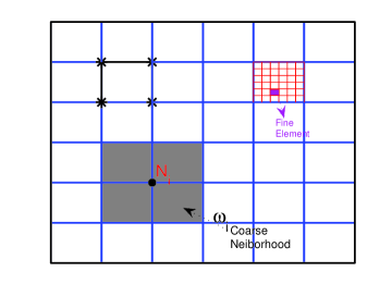
Figure 4.2: Illustration of the discretization configuration. The computational domain $\Omega$ is equipped with a coarse mesh partition (the element marked by $\ast$) and a fine mesh partition (depicted by the red lines for a coarse element). The gray region illustrates the neighborhood $\omega_{i}$ associated with the coarse node $N_{i}$.

We assume that the computational domain $\Omega$ is partitioned uniformly by a coarse mesh $\mathcal{T}_{H}$ and a fine mesh $\mathcal{T}_{h}$, with mesh size $H$ and $h$, respectively. Moreover, $\mathcal{T}_{h}$ is obtained by refining the coarse mesh $\mathcal{T}_{H}$. The nodes of the the coarse mesh are denoted by $\{N_{i}\}^{\mathcal{N}_{c}}_{i=1}$, where $\mathcal{N}_{c}$ represents the number of coarse nodes. The neighborhood $\omega_{i}$ of the node $N_{i}$ consists of all the coarse mesh elements for which node $N_{i}$ is a vertex, i.e.,

$$\omega_{i}=\cup\{K_{s}\in\mathcal{T}_{H}|x_{i}\in\overline{K_{s}}\}.$$

Generalized multiscle finite element method uses two stages: offline stage and online stage. At the offline stage of GMsFEM, we firstly construct the space of “snapshots”, $V^{(i)}_{snap}$, and then introduce the construction of local reduced basis functions. For the snapshot space, we can construct it by various ways [15]: (1) all fine-grid functions; (2) harmonic snapshots; (3) oversampling harmonic snapshots; and (4) forced-based snapshots. In this paper, we adopt the second choice to form a snapshot space. For each fine-grid function $\delta^{h}_{j}(x)$, which is defined by $\delta^{h}_{j}(x_{k})=\delta_{j,k}$, $\forall j,k\in J_{h}(\omega_{i})$, where $J_{h}(\omega_{i})$ denotes the fine-grid nodes on the boundary $\partial\omega_{i}$. We obtain a snapshot function $\zeta^{\omega_{i}}_{j}(x)$ by solving

$$\mathcal{L}(\zeta^{\omega_{i}}_{j}(x))=0~{}\text{in}~{}\omega_{i}$$

with the boundary condition, $\zeta^{\omega_{i}}_{j}(x)=\delta^{h}_{j}(x)$ on $\partial\omega_{i}$, and $\delta_{j,k}=1$ if $j=k$ and $\delta_{j,k}=0$ if $j\neq k$. Here, $\mathcal{L}$ is the differential operator corresponding to the state equation and adjoint equation in (2.4). For brevity of notation we now omit the superscript $\omega_{i}$, yet it is assumed throughout this section that the local reduced space computations are localized to respective coarse subdomains. We let $l_{i}$ be the number of functions in the snapshot space, and

$$V_{snap}(\omega_{i})=\text{span}\{\zeta_{j}(x),1\leq j\leq l_{i}\},$$

for each subregion $\omega_{i}$. Components of $V_{snap}$ are linear combinations of the fine-grid basis functions with coefficients stored in $R_{snap}$, i.e.,

$$R_{snap}=[\zeta_{1},\zeta_{2},\cdots,\zeta_{l_{i}}.]$$

After obtaining the snapshot space $V_{snap}$, we move on to the construction of the local reduced space $V_{lr}(\Omega)$ following the similar procedure. We will solve local eigenvalue problem in the snapshot space $V_{snap}(\omega_{i})$. Given the neighborhood $\omega_{i}$, the local eigenvalue problem is defined by

$$\begin{split}A^{lr}\phi^{lr}_{i,\ell}=\lambda_{\ell}S^{lr}\phi^{lr}_{i,\ell}.\end{split}$$ (4.27)

If the state equation is a diffusion equation with diffusion coefficient $\kappa(x)$, we specify the matrixes in (4.27) by

$$A^{lr}:=[a^{lr}_{mn}]=\int_{\omega_{i}}\kappa(x)\nabla\zeta_{m}\nabla\zeta_{n}dx,\quad S^{lr}:=[s^{lr}_{mn}]=\int_{\omega_{i}}\kappa(x)\zeta_{m}\zeta_{n}dx.$$

To accelerate the procedure of solving the local eigenvalue problem, we can replace the coefficient $\kappa(x)$ by $\widetilde{\kappa(x)}=\sum\limits^{\mathcal{N}_{c}}_{i=1}H^{2}|\nabla\chi_{i}|^{2}$ and $\{\chi_{i}\}$ is a set of partition of unity functions [2, 3] corresponding to the grid the grid $\mathcal{T}_{H}$.

Let $\{L_{p}(x)\}$ be the standard basis functions defined on the fine mesh, which belong to the FE approximation space $V_{h}(\Omega)$. Since the snapshot functions in $V_{snap}(\omega_{i})$ can be represented by the linear combinations of standard basis functions, $A^{lr}$ and $S^{lr}$ can be written as

$$A^{lr}=(R_{snap})^{T}AR_{snap}\quad and\quad S^{lr}=(R_{snap})^{T}SR_{snap},$$

respectively. Here $A$ and $S$ are the counterparts of $A^{lr}$ and $S^{lr}$ built with the fine-grid basis functions with the following expressions:

$$A:=[a_{pq}]=\int_{\omega_{i}}\kappa(x)\nabla L_{p}\nabla L_{q}dx\quad and\quad S:=[s_{pq}]=\int_{\omega_{i}}\kappa(x)L_{p}L_{q}dx.$$

We then let $\lambda^{i}_{1}\leq\lambda^{i}_{2}\leq\cdots$ be the eigenvalues and let $\phi^{lr}_{i,1},\phi^{lr}_{i,2},\cdots$ be the corresponding eigenvectors. Finally, we downscale the eigenvectors generated by snapshot functions to local fine scale solution by using basis functions in $V_{snap}$ and denote the eigenfunctions by $\{\rho_{i,\ell}\}$ on local fine grid $\omega_{i}$.

We note that $\{\zeta_{m}(x)\}$ (or $\{L_{m}(x)\}$) are functions of the spatial variables $x$, whereas $\{\phi^{lr}_{i,\ell}\}$ (or $\{\rho_{i,\ell}\}$) are discrete vectors. The linear combination of the snapshot functions (or the fine grid basis functions), i.e., $\zeta^{i,\ell}$ (or $L^{i,\ell}$ ), with $\phi^{lr}_{i,\ell}$ (or $\rho_{i,\ell}$) as the coefficient vector can be understood as the eigenfunction of the continuous problem corresponding to (4.27).

The number of eigenvectors that satisfy (4.27) is the same as the number of the fine-grid basis functions defined on the neighborhood $\omega_{i}$. However, we only retain a few of them that correspond to the smallest eigenvalues. We choose the $M_{i}$ lowermost eigenvalues and the corresponding eigenvectors of the eigenvalue problem (4.27), i.e. the eigenvalues and eigenvectors denoted by $\{\lambda^{(i)}_{\ell}\}^{M_{i}}_{\ell=1}$ and $\{\rho^{(i)}_{\ell}\}^{M_{i}}_{\ell=1}$. The local reduced space $V^{(i)}_{lr}:=\{\rho^{(i)}_{\ell},1\leq\ell\leq M_{i}\}$ on the local region $\omega_{i}$. We use partition of unity functions $\{\chi_{i}\}$ to paste the snapshot functions and get the multiscale basis function space

$$V_{lr}(\Omega):=\text{span}\{\rho_{k}:1\leq k\leq M\}=\text{span}\{\rho_{i,\ell}:\rho_{i,\ell}=\chi_{i}\rho^{(i)}_{\ell},1\leq i\leq\mathcal{N}_{c},1\leq\ell\leq M_{i}\},$$

where $M=\sum\limits^{\mathcal{N}_{c}}_{i=1}M_{i}$ is the total number of eigenvectors for reduced space. Components of $V_{lr}$ are linear combinations of the fine-grid basis functions with coefficients stored in $R^{l}$, i.e.,

$$R^{l}=[\rho_{1},\rho_{2},\cdots,\rho_{M}].$$ (4.28)

At the online stage, the multiscale basis functions can be repeatedly used. Compared with direct numerical simulation on fine grid, GMsFEM can significantly improve the computation efficiency.

We note that GMsFEM is only applied to the approximation space for state variable and adjoint variable. While for control variable, we do not use GMsFEM approximation.

5 Local-global model reduction method

In this section, we will discuss the construction of the local-global model reduction framework and present a greedy algorithm to get the optimal samples from a training set.

5.1 Local-global model reduction method for optimality system

We apply local model reduction method into the optimality system (3.11), i.e., finding $u_{l}(\mu)\in\mathscr{V}_{lr}(\Omega)$, $f_{l}(\mu)\in\mathcal{M}_{h}(\Omega)$, $\lambda_{l}(\mu)\in\mathscr{V}_{lr}(\Omega)$ such that

$$\begin{cases}\begin{split}a(u_{l},\widetilde{u}_{l};\mu)&=(f_{l},\widetilde{u}_{l};\mu)~{}\forall\widetilde{u}_{l}\in\mathscr{V}_{lr}(\Omega),\\ a(\lambda_{l},\widetilde{\lambda}_{l};\mu)&=-(u_{l}-\hat{u},\widetilde{\lambda}_{l};\mu)~{}\forall\widetilde{\lambda}_{l}\in\mathscr{V}_{lr}(\Omega),\\ 2\beta(f_{l},\widetilde{f}_{l};\mu)&=(\widetilde{f}_{l},\lambda_{l};\mu)~{}\forall\widetilde{f}_{l}\in\mathcal{M}_{h}(\Omega).\end{split}\end{cases}$$ (5.29)

Here $\mathscr{V}_{lr}(\Omega):=L^{2}_{\rho}(\Gamma)\otimes V_{lr}(\Omega)\subset\mathscr{V}_{h}(\Omega)$.

In the matrix notation, the reduced optimality matrix corresponding to (5.29) is defined by

$$\underbrace{\left[\begin{array}[]{ccc}2\beta M_{1}(\mu)&0&-M^{T}_{2}(\mu)R^{l}\\ 0&(R^{l})^{T}M_{3}(\mu)R^{l}&(R^{l})^{T}K^{T}(\mu)R^{l}\\ -(R^{l})^{T}M_{2}(\mu)&(R^{l})^{T}K(\mu)R^{l}&0\end{array}\right]}\limits_{\Lambda_{l}(\mu)\in\mathbb{R}^{(N_{e}+2M)\times(N_{e}+2M)}}\left[\begin{array}[]{c}\vec{F}_{l}(\mu)\\ \vec{u}_{l}(\mu)\\ \vec{\lambda}_{l}(\mu)\end{array}\right]=\left[\begin{array}[]{c}0\\ (R^{l})^{T}\widehat{U}\\ (R^{l})^{T}d\end{array}\right].$$ (5.30)

Here if we set

$$R=\left[\begin{array}[]{ccc}I&0&0\\ 0&(R^{l})^{T}&0\\ 0&0&(R^{l})^{T}\\ \end{array}\right]\in\mathbb{R}^{(N_{e}+2M)\times(N_{e}+2N_{h})},$$

then $\Lambda_{l}(\mu)=R\Lambda_{l}(\mu)R^{T}$. Thus,

$$u_{l}(\mu)=(R^{l})^{T}\vec{u}_{l}(\mu),\quad f_{l}(\mu)=(R^{l})^{T}\vec{F}_{l}(\mu),\quad\lambda_{l}(\mu)=(R^{l})^{T}\vec{\lambda}_{l}(\mu).$$

Similarly in Section 4.1, we can define the local-global reduced spaces for the state, control, adjoint variables, respectively, by

$$\begin{split}\begin{cases}X^{N}_{l}(\Omega)=\text{span}\{u_{l}(\mu^{n}),1\leq n\leq N\}\\ Y^{N}_{l}(\Omega)=\text{span}\{f_{l}(\mu^{n}),1\leq n\leq N\}\\ Z^{N}_{l}(\Omega)=\text{span}\{\lambda_{l}(\mu^{n}),1\leq n\leq N\}.\end{cases}\end{split}$$ (5.31)

Moreover, we define the enriched space by

$$Q^{N}_{lg}(\Omega)=X^{N}_{l}(\Omega)\cup Z^{N}_{l}(\Omega)=\text{span}\{u_{l}(\mu^{n}),\lambda_{l}(\mu^{n}),1\leq n\leq N\},$$

and set

$$X^{N}_{lg}(\Omega)=Q^{N}_{lg}(\Omega),\quad Y^{N}_{lg}(\Omega)=Y^{N}_{l}(\Omega),\quad Z^{N}_{lg}(\Omega)=Q^{N}_{lg}(\Omega),\quad\mathcal{U}^{N}_{lg}(\Omega)=X^{N}_{lg}(\Omega)\times Y^{N}_{lg}(\Omega).$$

On the low-dimensional subspace $\mathscr{U}^{N}_{lg}(\Omega)\times Z^{N}_{lg}(\Omega)$, the local-global reduced approximation is: for $\forall\mu\in\Gamma$, find $(\underline{u}^{N}_{lg},\lambda^{N}_{lg})\in\mathscr{U}^{N}_{lg}(\Omega)\times Z^{N}_{lg}(\Omega)$ such that

$$\begin{cases}\begin{split}\mathcal{A}(\underline{u}_{lg},\underline{v}_{lg})+\mathcal{B}(\underline{v}_{lg},\lambda_{lg})&=(\underline{\hat{u}},\underline{v}_{lg})\quad\forall\underline{v}_{lg}\in\mathscr{U}^{N}_{lg},\\ \mathcal{B}(\underline{u}_{lg},\widetilde{u}_{lg})&=(g,\widetilde{u}_{lg})_{\partial\Omega}\quad\forall\widetilde{u}_{lg}\in Z^{N}_{lg}(\Omega).\end{split}\end{cases}$$ (5.32)

In a similar way, we can show the continuity and coercivity properties for the local-global reduced saddle point problem (5.32).

The corresponding optimality system is: for $\forall\mu\in\Gamma$, find $(u^{N}_{lg},f^{N}_{lg},\lambda^{N}_{lg})\in X^{N}_{lg}(\Omega)\times Y^{N}_{lg}(\Omega)\times Z^{N}_{lg}(\Omega)$ such that

$$\begin{cases}\begin{split}a(u_{lg},\widetilde{u}_{lg};\mu)&=(f_{lg},\widetilde{u}_{lg};\mu)~{}\forall\widetilde{u}_{lg}\in X^{N}_{lg}(\Omega),\\ a(\lambda_{lg},\widetilde{\lambda}_{lg};\mu)&=-(u_{lg}-\hat{u},\widetilde{\lambda}_{lg};\mu)~{}\forall\widetilde{\lambda}_{lg}\in Z^{N}_{lg}(\Omega),\\ 2\beta(f_{lg},\widetilde{f}_{lg};\mu)&=(\widetilde{f}_{lg},\lambda_{lg};\mu)~{}\forall\widetilde{f}_{lg}\in Y^{N}_{lg}(\Omega).\end{split}\end{cases}$$ (5.33)

Let $\{\tau_{j}\}^{2N}_{j=1}=\{u_{l}(\mu^{n})\}^{N}_{n=1}\cup\{\lambda_{l}(\mu^{n})\}^{N}_{n=1}$ such that $Q^{N}_{lg}(\Omega)=\text{span}\{\tau_{j},j=1,\cdots,2N\}$, and we can express the local-global reduced state, adjoint, and control solutions as

$$\begin{split}\begin{cases}u_{lg}=\sum\limits^{2N}_{i=1}u^{i}_{lg}\tau_{i}=\sum\limits^{2N}_{i=1}\sum\limits^{2M}_{k=1}u^{i}_{lg}Z^{i}_{1,k}\rho_{k}=\sum\limits^{2N}_{i=1}\sum\limits^{2M}_{k=1}\sum\limits^{N_{h}}_{n=1}u^{i}_{lg}Z^{i}_{1,k}R_{k,n}\psi_{n},\\ f_{lg}=\sum\limits^{N}_{j=1}f^{j}_{lg}f_{l}(\mu^{j})=\sum\limits^{N}_{j=1}\sum\limits^{N_{e}}_{\ell=1}f^{j}_{lg}Z_{2,\ell}\phi_{\ell},\\ \lambda_{lg}=\sum\limits^{2N}_{m=1}\lambda^{m}_{lg}\tau_{m}=\sum\limits^{2N}_{m=1}\sum\limits^{2M}_{n=1}\lambda^{m}_{lg}Z^{m}_{1,n}\rho_{n}=\sum\limits^{2N}_{m=1}\sum\limits^{2M}_{n=1}\sum\limits^{N_{h}}_{s=1}\lambda^{m}_{lg}Z^{m}_{1,n}R_{n,s}\psi_{s}.\end{cases}\end{split}$$

With the affine assumption (3.9), we can get the similar linear system to (4.23) in the local-global reduced case. Hence, given a random sample $\mu$, the reduced linear system associated to the system (5.33) can be written as:

$$\underbrace{\left[\begin{array}[]{ccc}2\beta M_{1,lg}(\mu)&0&-M^{T}_{2,lg}(\mu)\\ 0&M_{3,lg}(\mu)&K^{T}_{lg}(\mu)\\ -M_{2,lg}(\mu)&K_{lg}(\mu)&0\end{array}\right]}\limits_{\Lambda_{N}(\mu)\in\mathbb{R}^{5N\times 5N}}\left[\begin{array}[]{c}F_{lg}(\mu)\\ u_{lg}(\mu)\\ \lambda_{lg}(\mu)\end{array}\right]=\left[\begin{array}[]{c}0\\ \overline{\widehat{U}}_{lg}\\ d_{lg}\end{array}\right].$$ (5.34)

With the definition of the basis matrix:

$$\mathcal{Z}=\left[\begin{array}[]{ccc}\mathcal{Z}^{T}_{2}&0&0\\ 0&\mathcal{Z}^{T}_{1}&0\\ 0&0&\mathcal{Z}^{T}_{1}\\ \end{array}\right]\in\mathbb{R}^{5N\times(N_{e}+2M)},$$

$\Lambda_{N}(\mu)$ is given by $\Lambda_{N}(\mu)=\mathcal{Z}(R\Lambda(\mu)R^{T})\mathcal{Z}^{T}$. Although being dense rather than sparse as in the FE case, the system matrix $\Lambda_{N}(\mu)$ is very small and still symmetric with saddle-point structure. Finally, we can downscale the local-global reduced solutions to fine scale solution by

$$\vec{u}_{lg}(\mu)=Z_{1}R_{l}u_{lg}(\mu),\quad\vec{f}_{lg}(\mu)=Z_{2}f_{lg}(\mu),\quad\vec{\lambda}_{lg}(\mu)=Z_{1}R_{l}\lambda_{lg}(\mu).$$

5.2 Sampling strategy

In order to find a few optimal parameter samples $\mu^{n},1\leq n\leq N$ to construct the hierarchical Lagrange RB approximation spaces and to assure the fidelity of the reduced model to approximate the original model, we use the sampling strategy based on the greedy algorithm [41, 39]. We denote the finite-dimensional sample set by $\Xi_{train}\subset\Gamma$. The cardinality of $\Xi_{train}$ will be denoted $|\Xi_{train}|=n_{train}$ and we assume that $\Xi_{train}$ is a good surrogate for the set $\Gamma$. The idea of the greedy procedure is that, starting with a train sample $\Xi_{train}$, we adaptively select $N_{max}$ parameters $\mu_{1},\cdots,\mu_{N_{max}}$ and form the hierarchical sequence of RB spaces $X^{N}_{lg}(\Omega),Y^{N}_{lg}(\Omega),Z^{N}_{lg}(\Omega)$. At the $N-$th iteration, the greedy algorithm enriches the retained snapshots by a particular candidate snapshot over all candidates snapshots $(u_{l}(\mu),f_{l}(\mu),\lambda_{l}(\mu)),\mu\in\Xi_{train}$, which is least well approximated by $X^{N-1}_{lg}(\Omega)\times Y^{N-1}_{lg}(\Omega)\times\lambda^{N-1}_{lg}(\Omega)$.

Firstly, we consider the residual errors for local reduced model. By the first equation of system (5.29), we can get

$$a(u_{l}-u^{N}_{l}+u^{N}_{l},\widetilde{u}_{l};\mu)=(f_{l}-f^{N}_{l}+f^{N}_{l};\mu),\quad\forall\widetilde{u}_{l}\in\mathscr{V}_{lr}(\Omega),$$

that is,

$$a(u_{l}-u^{N}_{l},\widetilde{u}_{l};\mu)-(f_{l}-f^{N}_{l},\widetilde{u}_{l};\mu)=-a(u^{N}_{l},\widetilde{u}_{l};\mu)+(f^{N}_{l},\widetilde{u}_{l};\mu),\quad\forall\widetilde{u}_{l}\in\mathscr{V}_{lr}(\Omega).$$

Let the error $e_{u}(\mu):=u_{l}(\mu)-u^{N}_{l}(\mu),e_{f}(\mu):=f_{l}(\mu)-f^{N}_{l}(\mu)$ and $r_{1}(\widetilde{u}_{l};\mu)\in\mathscr{V}^{*}_{lr}(\Omega)$ (the dual space of $\mathscr{V}_{lr}(\Omega)$) be the residual

$$r_{1}(\widetilde{u}_{l};\mu)=-a(u^{N}_{l},\widetilde{u}_{l};\mu)+(f^{N}_{l},\widetilde{u}_{l};\mu),\quad\forall\widetilde{u}_{l}\in\mathscr{V}_{lr}(\Omega).$$

Then we can obtain

$$a(e_{u}(\mu),\widetilde{u}_{l};\mu)-(e_{f}(\mu),\widetilde{u}_{l};\mu)=r_{1}(\widetilde{u}_{l};\mu).$$

By the Riesz representation theory, there exists a function $\hat{e}_{1}(\mu)$ such that

$$(\hat{e}_{1}(\mu),\widetilde{u}_{l})_{\mathscr{V}_{l}}=r_{1}(\widetilde{u}_{l};\mu),\quad\forall\widetilde{u}_{l}\in\mathscr{V}_{lr}(\Omega).$$ (5.35)

Consequently, the dual norm of the residual $r_{1}(\widetilde{u}_{l};\mu)$ can be evaluated by the Riesz representation,

$$\|r_{1}(\widetilde{u}_{l};\mu)\|_{\mathscr{V}^{*}_{lr}}:=\sup_{\widetilde{u}_{l}\in\mathscr{V}_{lr}}\frac{r_{1}(\widetilde{u}_{l};\mu)}{\|\widetilde{u}_{l}\|_{\mathscr{V}_{lr}}}=\|\hat{e}_{1}(\mu)\|_{\mathscr{V}_{lr}}.$$

The computation of the residual is important to perform the offline-online computation decomposition. Combined by (3.9) and (4.20), the residual can be expressed as

$$\begin{split}r_{1}(\widetilde{u}_{l};\mu)&=-a(u^{N}_{l},\widetilde{u}_{l};\mu)+(f^{N}_{l},\widetilde{u}_{l};\mu)\\ &=-\sum^{2N}_{i=1}u^{\mathcal{N}}_{i}(\mu)a(\delta_{i},\widetilde{u}_{l};\mu)+\sum^{N}_{j}f^{\mathcal{N}}_{j=1}(\mu)(\xi_{j},\widetilde{u}_{l})\\ &=-\sum^{Q_{a}}_{q=1}\sum^{2N}_{i=1}\theta_{q}(\mu)u^{\mathcal{N}}_{i}(\mu)a_{q}(\delta_{i},\widetilde{u}_{l})+\sum^{N}_{j=1}f^{\mathcal{N}}_{j=1}(\mu)(\xi_{j},\widetilde{u}_{l}).\end{split}$$ (5.36)

By (5.35) and (5.36), we have

$$(\hat{e}_{1}(\mu),\widetilde{u}_{l})_{\mathscr{V}_{lr}}=-\sum^{Q_{a}}_{q=1}\sum^{2N}_{i=1}\theta_{q}(\mu)u^{\mathcal{N}}_{i}(\mu)a_{q}(\delta_{i},\widetilde{u}_{l})+\sum^{N}_{j=1}f^{\mathcal{N}}_{j}(\mu)(\xi_{j},\widetilde{u}_{l}).$$

This implies that

$$\begin{split}\hat{e}_{1}(\mu)=-\sum^{Q_{a}}_{q=1}\sum^{2N}_{i=1}\theta_{q}(\mu)u^{\mathcal{N}}_{i}(\mu)L^{\delta}_{i}+\sum^{N}_{j=1}f^{\mathcal{N}}_{j}(\mu)L^{\xi}_{j},\end{split}$$ (5.37)

where $L^{\delta}_{i},L^{\xi}_{j}$ are Riesz representations of $a_{q}(\delta_{i},\widetilde{u}_{l})$ and $(\xi_{j},\widetilde{u}_{l})$, i.e., $(L^{\delta}_{i},\widetilde{u}_{l})_{\mathscr{V}_{lr}}=a_{q}(\delta_{i},\widetilde{u}_{l})$ and $(L^{\xi}_{j},\widetilde{u}_{l})_{\mathscr{V}_{lr}}=(\xi_{j},\widetilde{u}_{l})$ for all $\widetilde{u}_{l}\in\mathscr{V}_{lr}(\Omega)$, respectively. We thus obtain

$$\begin{split}\|\hat{e}_{1}(\mu)\|^{2}_{\mathscr{V}_{lr}}&=\sum^{Q_{a}}_{q=1}\sum^{Q_{a}}_{q^{\prime}=1}\sum^{2N}_{i=1}\sum^{2N}_{i^{\prime}=1}\theta_{q}(\mu)\theta_{q^{\prime}}(\mu)u^{\mathcal{N}}_{i}u^{\mathcal{N}}_{i^{\prime}}(L^{\delta}_{i},L^{\delta}_{i^{\prime}})_{\mathscr{V}_{lr}}\\ &+\sum^{N}_{j=1}\sum^{N}_{j^{\prime}=1}f^{\mathcal{N}}_{j}(\mu)f^{\mathcal{N}}_{j^{\prime}}(\mu)(L^{\xi}_{j},(L^{\xi}_{j^{\prime}})_{\mathscr{V}_{lr}}-2\sum^{Q_{a}}_{q=1}\sum^{2N}_{i=1}\sum^{N}_{j=1}\theta_{q}(\mu)f^{\mathcal{N}}_{j}(\mu)(L^{\delta}_{i},L^{\xi}_{j})_{\mathscr{V}_{lr}}.\end{split}$$ (5.38)

Combining (5.35) and (5.38) gives the calculation of the dual norm of the residual $\|r_{1}(\widetilde{u}_{l};\mu)\|_{\mathscr{V}^{*}_{lr}}$. With the similar way, we can define residuals $r_{2}(\widetilde{\lambda}_{l};\mu)$ and $r_{3}(\widetilde{f}_{l};\mu)$ for the rest equations of system (5.29) with the corresponding functions $\hat{e}_{2}(\mu)$ and $\hat{e}_{3}(\mu)$.

Next, we define the error estimator as

$$\begin{split}\vartriangle_{N}(\mu)&=\bigg{(}\|r_{1}(\widetilde{u}_{l};\mu)\|^{2}_{\mathscr{V}^{*}_{lr}}+\|r_{2}(\widetilde{u}_{l};\mu)\|^{2}_{\mathscr{V}^{*}_{lr}}+\|r_{3}(\widetilde{u}_{l};\mu)\|^{2}_{L^{2}}\bigg{)}^{\frac{1}{2}}\\ &=(\|\hat{e}_{1}(\mu)\|^{2}_{\mathscr{V}_{lr}}+\|\hat{e}_{2}(\mu)\|^{2}_{\mathscr{V}_{lr}}+\|\hat{e}_{3}(\mu)\|^{2}_{L^{2}})^{\frac{1}{2}}.\end{split}$$ (5.39)

Let $\varepsilon^{*}_{tol}$ be a chosen tolerance for the stopping criterium. The greedy sampling strategy is described in Algorithm 1.

Algorithm 1 Greedy algorithm for selecting optimal parameter samples $S_{N}$

Input: A training set $\Xi_{train}\subset\Gamma$, a tolerance $\varepsilon^{*}_{tol}$, a maximum number $N_{max}$
Output: $S_{N}$ and $X^{N}_{lg},Y^{N}_{lg},Z^{N}_{lg}$
 1:   Initialization: $\mu_{1}=\text{mean}(\Xi_{train})$, $S_{1}=\{\mu_{1}\}$;
 2:   compute $u_{l}(\mu_{1}),f_{l}(\mu_{1}),\lambda_{l}(\mu_{1})$ by local model reduction method;
 3:   obtain $X^{1}_{lg}=\text{span}\{u_{l}(\mu_{1}),\lambda_{l}(\mu_{1})\}$, $Y^{1}_{lg}=\text{span}\{f_{l}(\mu_{1})\}$, $Z^{1}_{lg}=X^{1}_{lg}$;
 4:   $\Xi_{train}$ = $\Xi_{train}\setminus\mu_{1}$;
 6:   apply Gram-Schmidt process to $X^{1}_{lg}$, $Y^{1}_{lg}$, $Z^{1}_{lg}$;
 7:   $\varepsilon_{1}=\max\limits_{\mu\in\Xi_{train}}\vartriangle_{1}(\mu)$;
 8:   N=1;
 9:   $\mathbf{while}~{}\varepsilon_{N}\leq\varepsilon^{*}_{tol}$ or $N\leq N_{max}$
 10:   $N=N+1$;
 11:   $\mu_{N}=\text{argmax}_{\mu\in\Xi_{train}}\vartriangle_{N-1}(\mu)$;
 12:   $S_{N}=S_{N-1}\cup\{\mu_{N}\}$;
 13:   compute $u_{l}(\mu_{N}),f_{l}(\mu_{N}),\lambda_{l}(\mu_{N})$ by local model reduction method;
 14:   update the reduced spaces $X^{N}_{lg}=X^{N-1}_{lg}\cup\text{span}\{u_{l}(\mu_{N}),\lambda_{l}(\mu_{N})\}$,
      $f^{N}_{lg}=f^{N-1}_{lg}\cup\text{span}\{f_{l}(\mu_{N})\}$, $Z^{N}_{lg}=X^{N}_{lg}$;
 15:   apply Gram-Schmidt process to $X^{N}_{lg}$, $Y^{N}_{lg}$, $Z^{N}_{lg}$;
 16:   $\Xi_{train}$ = $\Xi_{train}\setminus\mu_{N}$;
 17:   $\varepsilon_{N}=\max\limits_{\mu\in\Xi_{train}}\vartriangle_{N}(\mu)$;
end while

With the model reduction framework shown in Section 5.1 and the above greedy sampling strategy, we outline the local-global model reduction method in algorithm 2.

Algorithm 2 Local-global model reduction method for stochastic optimal control problems.

Input: Training set $\Xi_{train}\subset\Gamma$, Testing set $\Xi_{test}\subset\Gamma$
Offline Stage:
 1:   get spaces $X^{N}_{lg}(\Omega),Y^{N}_{lg}(\Omega),Z^{N}_{lg}(\Omega)$ by Algorithm 1;
 2:   calculate the local reduced matrix $R$ and the global reduced matrix $Z$;
 3:   if affine assumptions (3.9) holds, then
      compute the $\mu$-independent matrices $K^{q}_{h}$, $M_{1,h}$, $M_{2,h}$, $M_{3,h}$ and $\mu$-independent load vectors
      $\widehat{U}_{p}$ in (3.13);
      else
      use EIM to $a(\cdot,\cdot;\mu)$ and $(f,\cdot;\mu)$;
 4:   Go back to the step 4;
      end if
Online Stage: For the $k_{th}$ test parameter $\mu_{k}$ in $\Xi_{test}$
 5:   update the $\mu$-dependent coefficients $Q^{q}_{a}(\mu_{k})$, $\widehat{u}_{p}(\mu_{k})$ in (3.13);
 6:   assemble the full matrix $\Lambda_{h}(\mu_{k})$ and right term $[0;\overline{\widehat{U}};d]^{T}$;
 7:   compute the reduced matrix $\Lambda_{N}(\mu_{k})$ and the reduced right hand $[0;\overline{\widehat{U}}_{lg};d_{lg}]^{T}$;
 8:   solve the system (5.34) for the reduced solutions $u_{lg}(\mu_{k})$, $F_{lg}(\mu_{k})$, $\lambda_{lg}(\mu_{k})$;
 9:   get the local-global RB solutions $\vec{F}_{lg}(\mu_{k})$, $\vec{u}_{lg}(\mu_{k})$ , $\vec{\lambda}_{lg}(\mu_{k})$ defined on fine grid;

In the paper, we have focused on the global existence and uniqueness of the optimal solution and the local-global model reduction framework for the distributed optimal control problem. The existence and uniqueness of global optimal solution for boundary optimal control problem can be proved in a similar way, and the local-global model reduction method can also be used in the boundary optimal control problem. We present a numerical example for the boundary optimal control problem in Section 6.3.

6 Numerical experiments

A variety of numerical examples are presented to demonstrate the efficiency of the local-global model reduction method for stochastic optimal control problems. In this section, we focus on stochastic optimal control problems constrained by elliptic PDEs. In the following, we are going to show the relative errors and computation performance for the control, state, and adjoint variables. In Section 6.1, we consider the stochastic optimal control problem, where the diffusion coefficient and target function are both random fields. The effect of the regularization parameter $\beta$ will be discussed. In Section 6.2, we consider the control problem which is defined on a random domain. The last example in Section 6.3, we compute a Neumann boundary control problem with the local-global model reduction method. In this case, the diffusion coefficient and target function are random fields with high dimensional parameters. To demonstrate the efficiency of our presented model reduction method, we will list the detailed CPU time in the last two examples.

6.1 Stochastic optimal control problem defined on deterministic domain

In the first example, we consider the target function $\hat{u}(x,\mu)$ and coefficient $\kappa(x,\mu)$ are both related to the parameter sample $\mu\in\Gamma$ and numerically explore the approximation of optimal solution using the local-global model reduction method.

The computational domain is a two-dimensional unit square $\Omega=[0,1]^{2}$. We consider the optimal control problem

$$\begin{cases}\begin{split}&\min\limits_{u,f}J=\frac{1}{2}\|u(x,\mu)-\hat{u}(x,\mu)\|^{2}_{\mathscr{L}^{2}(\Omega)}+\beta\|f(x,\mu)\|^{2}_{\mathscr{L}^{2}(\Omega)}\\ &s.t.~{}~{}-div(\kappa(x,\mu)\nabla u)=f(x,\mu)~{}\text{in}~{}\Omega\\ &\quad\quad\quad u|_{\partial\Omega}=g(x),\end{split}\end{cases}$$ (6.40)

where the diffusion coefficient $\kappa(x,\mu)$ and the desired state function $\hat{u}(x,\mu)$ are

$$\begin{cases}\begin{split}\kappa(x,\mu)&=(\mu^{2}+(\mu+0.5)^{2})\kappa_{1}(x)+(1+\exp(\mu)\cos(\mu/3))^{2}\kappa_{2}(x),\\ \hat{u}(x,\mu)&=x_{1}x_{2}(x_{1}+1)(x_{2}-1)\mu+x^{2}_{1}x_{2}(x_{1}-1)(x_{2}+1)\cos(\mu)\\ &\quad+x_{1}x^{3}_{2}(x_{1}-1)(x_{2}-1)\mu^{2}+\exp(x_{1}/3)x^{2}_{2}\sin(\mu).\end{split}\end{cases}$$

Here $x=(x_{1},x_{2})\in\Omega$ and the random variable $\mu\sim Beta(\theta_{1},\theta_{2})$ obey beta distribution with two shape parameters $\theta_{1},\theta_{2}\in\mathds{N}_{+}$. In this case, $(\theta_{1},\theta_{2})$ take the value (1,1). $\kappa_{1}(x)$ and $\kappa_{2}(x)$ are independent of $\mu$. The $\kappa_{1}(x)$ and $\kappa_{2}(x)$ are high-contrast functions and their maps are depicted in Fig. 6.3.

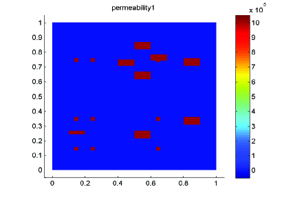
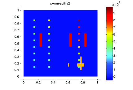
Figure 6.3: High-contrast coefficients $\kappa_{1}$ (left) and $\kappa_{2}$ (right).

In this example, we use $120\times 120$ uniform fine grid to compute the reference optimal solutions $(u_{ref},f_{ref},\lambda_{ref})$. The local-global model reduction solutions $(u_{lg},f_{lg},\lambda_{lg})$ are computed on $10\times 10$ coarse mesh. We define the relative errors for the state variable $u$, the control variable $f$ and the adjoint variable by

$$\begin{cases}\begin{split}&e^{2}_{u}=\frac{1}{N}\sum\limits^{N}_{i=1}\frac{\|u_{ref}(x,\mu_{i})-u_{lg}(x,\mu_{i})\|_{L^{2}(\Omega)}}{\|u_{ref}(x,\mu_{i})\|_{L^{2}(\Omega)}},\\ &e^{2}_{f}=\frac{1}{N}\sum\limits^{N}_{i=1}\frac{\|f_{ref}(x,\mu_{i})-f_{lg}(x,\mu_{i})\|_{L^{2}(\Omega)}}{\|f_{ref}(x,\mu_{i})\|_{L^{2}(\Omega)}},\\ &e^{2}_{\lambda}=\frac{1}{N}\sum\limits^{N}_{i=1}\frac{\|\lambda_{ref}(x,\mu_{i})-\lambda_{lg}(x,\mu_{i})\|_{L^{2}(\Omega)}}{\|\lambda_{ref}(x,\mu_{i})\|_{L^{2}(\Omega)}}.\\ \end{split}\end{cases}$$

The contour plot of the target solution $\hat{u}$ is given in Fig. 6.4, and contour plots of the control $f$ and the state $u$ for the three values of $\beta$ are given in Fig. 6.5. For the optimal control problem governed by PDE, the regularization parameter plays an important role. For small $\beta$, the control variable is not heavily penalized, and so the state may be closed to the desired state. However, given a large $\beta$, it is hard for the state variable to be near to the desired state in the relative $L^{2}$-norm because the input of control contributes more heavily into the cost functional. In Table 1, we demonstrate the relative $L^{2}$ errors about the state variable $u$ and the control variable $f$ for different $\beta$. Moreover, we compute the minimal values of cost functional. From the figures and the table, we can find that it is necessary to find a suitable regularization parameter for the optimal solution.

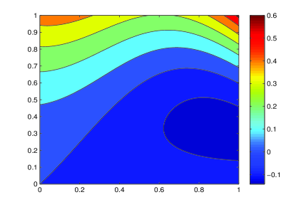
Figure 6.4: Contour plot of $\hat{u}(x,\mu)$ at the $\overline{\mu}$.

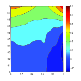
(a) u, $\beta=1\times 10^{-2}$

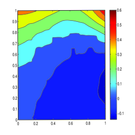
(b) u, $\beta=2\times 10^{-4}$

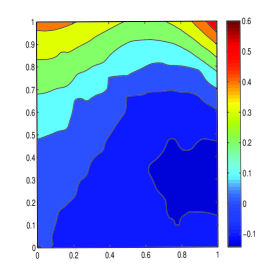
(c) u, $\beta=0.5\times 10^{-5}$

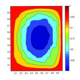
(d) f, $\beta=1\times 10^{-2}$

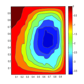
(e) f, $\beta=2\times 10^{-4}$

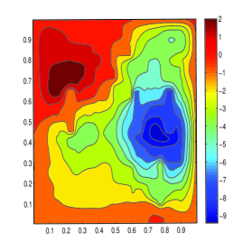
(f) f, $\beta=0.5\times 10^{-5}$

Figure 6.5: Contour plots of the state $u$, the control $f$ for $\beta=10^{-2}$, $2\times 10^{-4}$, $0.5\times 10^{-5}$.

$\beta$	$1\times 10^{-2}$	$2\times 10^{-4}$	$0.5\times 10^{-5}$
$e^{2}_{u}$	1.057E-02	1.033E-02	9.547E-03
$e^{2}_{f}$	1.779E-02	2.627E-02	5.586E-02
$J_{min}$	2.048E-02	3.974E-06	3.753E-05

Table 1: The relative $L^{2}$ errors with different regularization parameter $\beta$ for the state variable $u$, the control variable $f$ and the cost functional $J$.

Next we fix the regularization parameter $\beta$, the number of local basis functions $L$ for each coarse element and choose five global basis functions. To discuss the effect of coarse mesh size, we consider some different coarse mesh sizes in the example, $H=\{1/5,1/6,1/8,1/10,1/12\}$. The relative $L^{2}$ errors and the corresponding minimal values of cost functional are listed in Table 2. From the table, we can see that the approximation for the state variable $u$ and the control variable $f$ are improved as the coarse gird is refined. The minimal values of the cost functional $J$ get smaller as the coarse mesh becomes finer.

$Coarse~{}mesh~{}size$	$H=1/5$	$H=1/6$	$H=1/8$	$H=1/10$	$H=1/12$
$e^{2}_{u}$	5.229E-01	3.829E-01	2.425E-01	1.057E-02	7.743E-03
$e^{2}_{f}$	6.920E-01	7.117E-01	4.569E-01	1.779E-02	1.445E-02
$J_{min}$	4.003E-03	2.039E-03	9.756E-04	4.111E-04	4.103E-04

Table 2: The relative $L^{2}$ errors with different coarse mesh size $H$ for the state variable $u$, the control variable $f$ and the minimal value $J_{min}$.

6.2 Stochastic optimal control problem defined on random domain

In this subsection, we consider the stochastic optimal control problem described by (6.41) defined in a random domain $\Omega(\mu)=\{(x_{1},x_{2})|0\leq x_{1}\leq 1,s(x_{1},\mu)\leq x_{2}\leq 1,\mu\in\Gamma\}$, i.e.,

$$\begin{cases}\begin{split}&\min\limits_{u,f}J=\frac{1}{2}\|u(x,\mu)-\hat{u}(x)\|^{2}_{\mathscr{L}^{2}(\Omega(\mu))}+\beta\|f(x,\mu)\|^{2}_{\mathscr{L}^{2}(\Omega(\mu))},\\ &s.t.~{}~{}-div(\kappa(x)\nabla u)=f(x)~{}\text{in}~{}\Omega(\mu),\quad u|_{\partial\Omega}=g(x).\end{split}\end{cases}$$ (6.41)

Here the coefficient $\kappa(x)$ and target function $\hat{u}(x)$ are defined by

$$\kappa(x)=|x_{1}x_{2}|+1,\quad\hat{u}(x)=x_{1}x_{2}(x_{1}-1)(x_{2}-\frac{x_{1}}{2}-1)+1.$$

To be specific, we treat the rough bottom boundary as a random field $s(x_{1},\mu)$ with zero mean $\mathbb{E}(s(x_{1},\mu))=0$ and an exponential two-point covariance function

$$C_{s}(x_{1},z_{1})=\mathds{E}(s(x_{1},\mu),s(z_{1},\mu))=\exp(-|x_{1}-z_{1}|).$$

With the finite-term Karhunen-Lo$\grave{e}$ve expansion (K-L expansion), $s(x_{1},\mu)$ can be approximated by

$$s(x_{1},\mu)\approx\sigma\sum\limits^{N}_{n=1}\sqrt{\lambda_{n}}\phi_{n}(x)X_{n}(\omega),$$

where $\{(\lambda_{n},\phi_{n})\}^{N}_{n=1}$ are solutions of the eigenvalue problem,

$$\int_{\Gamma}C(x_{1},x_{2})\phi_{n}(x_{1})dx_{1}=\lambda_{n}\phi_{n}(x_{2}),\quad\forall x\in\Omega.$$

We set $\{X_{n}(\omega)\}\sim U(-1,1)$ to be independent uniform random variables and use the parameter $0<\sigma<1$ to control the maximum deviation of the rough surface.

In Fig. 6.6, we employ the K-L expansion to represent the random boundary and show some realizations of the boundary.

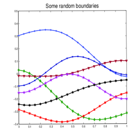
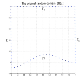
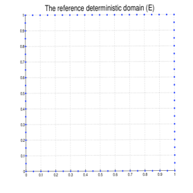
Figure 6.6: (a) 7 realizations of the bottom boundary $s(x_{1},\mu)$ generated by five-term K-L expansion; (b) a boundary realization in the physical domain $(x_{1},x_{2})$; (c) the mapped domain $(\xi_{1},\xi_{2})$.

To treat the random domain, we need to formulate a stochastic map [44]. The stochastic mapping of $\Omega(\mu)$ onto $E$ is constructed via the solutions of the Laplace equations,

$$\frac{\partial^{2}x_{1}}{\partial\xi^{2}_{1}}+\frac{\partial^{2}x_{1}}{\partial\xi^{2}_{2}}=0,\quad\frac{\partial^{2}x_{2}}{\partial\xi^{2}_{1}}+\frac{\partial^{2}x_{2}}{\partial\xi^{2}_{2}}=0\quad in~{}E,$$

subject to the boundary conditions

$$\begin{split}&x_{1}(0,\xi_{2})=x_{1}|_{\Gamma_{1}},\quad x_{1}(1,\xi_{2})=x_{1}|_{\Gamma_{3}}\\ &x_{1}(\xi_{1},0)=x_{1}|_{\Gamma_{4}},\quad x_{1}(\xi_{1},1)=x_{1}|_{\Gamma_{2}}\\ \end{split}$$

and

$$\begin{split}&x_{2}(0,\xi_{2})=x_{2}|_{\Gamma_{1}},\quad x_{2}(1,\xi_{2})=x_{2}|_{\Gamma_{3}}\\ &x_{2}(\xi_{1},0)=s(x_{1},\mu),\quad x_{2}(\xi_{1},1)=x_{2}|_{\Gamma_{2}},\\ \end{split}$$

where $x_{i}|_{\Gamma_{j}}$ denotes the $x_{i}$ coordinate along the boundary segment $\Gamma_{j}$. One can choose different distributions of boundary coordinates in $x$ as boundary conditions to achieve better computational results. With various methods to construct the stochastic map, the map is not bijective in general. Thus, we will describe all the numerical results on the mapped domain $E$.

We make $100\times 100$ fine grid to compute the reference solution and the number of degrees freedom $N_{f}=10201$ for fine scale FE method. The local model reduction computation (GMsFEM) is performed on the coarse grid $5\times 5$ with $180$ basis functions. For offline procedure, we select $100$ optimal samples for snapshot functions, i.e., $n_{train}=100$. Similar to the definition of $L^{2}$ error, we define the energy error by

$$e^{H}_{u}=\frac{1}{N}\sum\limits^{N}_{i=1}\frac{\|u_{ref}(x,\mu_{i})-u_{lg}(x,\mu_{i})\|_{a(E)}}{\|u_{ref}(x,\mu_{i})\|_{a(E)}}$$

The energy error $e^{H}_{\lambda}$ for the adjoint variable $\lambda$ can be defined similarly.

To evaluate the approximation for the local-global model reduction method, we randomly choose $1000$ parameter samples and compute the average relative $L^{2}$ errors and energy errors. For a fixed regularization parameter ($\beta=10^{-4}$) and five local-global basis functions, the mean and the variance of state and control variables are all shown in Fig. 6.7, where the first row represents for reference solutions of optimal control problem (6.41). With local-global model reduction method, the mean and variance for solutions are plotted in second row. From the figure, the moments of optimal control $f$ and the moments of state $u$ using local-global reduced method have a good agreement with the reference results.

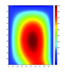
(a) ref-mean-state

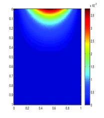
(b) ref-variance-state

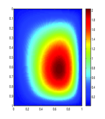
(c) ref-mean-control

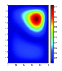
(d) ref-variance-control

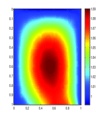
(e) mean of state

(f) variance of state

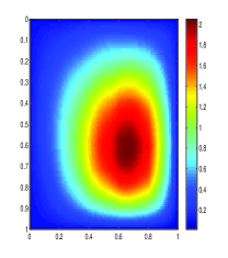
(g) mean of control

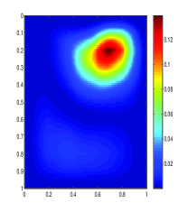
(h) variance of control

Figure 6.7: Mean and variance of reference solutions of (6.41) (1st row). Mean and variance of local-global reduced solutions (2nd row).

In Table 3 and Table 4, we list the number of optimal parameter samples for global model reduction method versus the relative error in the sense of $L^{2}$-norm and energy norm, respectively, for the state, control and adjoint variables.

Table 3: Average relative $L^{2}$ errors with different number of optimal parameter samples.

$N_{max}$	$2$	$3$	$4$	$5$	$6$	$7$	$8$
$e^{2}_{u}$	4.757E-03	4.264E-03	2.901E-03	1.373E-03	7.852E-04	7.610E-04	7.060E-04
$e^{2}_{f}$	1.807E-01	1.816E-01	1.553E-01	3.908E-02	2.764E-02	2.698E-02	2.485E-02
$e^{2}_{\lambda}$	1.808E-01	1.743E-01	1.663E-01	3.927E-02	2.704E-02	2.604E-02	2.422E-02

Table 4: Average relative $H^{1}$ errors with different number of optimal parameter samples.

$N_{max}$	$2$	$3$	$4$	$5$	$6$	$7$	$8$
$e^{H}_{u}$	5.992E-01	5.831E-01	3.908E-01	1.841E-01	1.533E-01	1.528E-01	1.510E-01
$e^{H}_{\lambda}$	2.758E-01	2.606E-01	2.626E-01	1.270E-01	1.154E-01	1.147E-01	1.124E-01

We see that, for a fixed number of local basis functions (L=5), the accuracy will improve as the number of optimal parameter samples (the number of global basis functions $N_{max}$) increases gradually. On the other hand, for the same optimal parameter samples ($N_{max}$=5), Table 5 shows that more local basis functions render a better approximation.

Table 5: Average relative $L^{2}$ errors for local-global model reduction method vs. different number of local basis functions.

$L$	$2$	$3$	$4$	$5$	$6$	$7$
$u_{lg}$	1.863E-03	1.720E-03	1.442E-03	1.373E-03	1.352E-03	1.304E-03
$f_{lg}$	4.958E-02	4.397E-02	4.303E-02	3.908E-02	3.880E-02	3.832E-02
$\lambda_{lg}$	4.829E-02	4.349E-02	4.303E-02	3.927E-02	3.893E-02	3.851E-02

Table 6: Computational details for the local-global reduced model for the stochastic optimal control problem defined on the random domain.

$\mathbf{Computation~{}setting}$		$\mathbf{local-global~{}reduced~{}model}$
Number of FE dofs $\mathcal{N}$	10201	Number of RB dofs	25
Number of parameters	5	Dofs reduction	1216:1
Error tolerance greedy $\epsilon^{*}_{tol}$	$10^{-5}$	Offline greedy time	1.704E+03 s
Number of local basis functions	5	Offline time for snapshot spaces	9.364E+02 s
Number of test parameters	1000	Online average time for optimal solutions	2.490E-02 s

In Table 6, we list the CPU time for the optimal control problem defined on the random domain with the high-fidelity model (FEM in fine grid) and the local-global reduced model. Before implementing the global reduced method, we need to compute the nested snapshots. As a sharp comparison, the local model reduction method only needs about 15 minutes to get the snapshot spaces, while the FE method in fine grid requires more than 65 hours for the snapshots. At the online stage, it takes 2.121s to get the optimal solutions for per parameter sample using the FE method. However, the online average time is only $2.490\text{E}-02s$ per sample. This shows that the local-global model reduction method can significantly improve the computational efficiency for the stochastic optimal control problem defined on random domain.

6.3 Stochastic optimal Neumann boundary control problem

Compared with the distributed control problems applied on the entire domain, boundary control problems have the control applied only on the boundary. Such boundary control problems are perhaps more physically realistic because for real-world applications, it may be possible to only control the physical property along the boundary of the domain. In this section, we consider the following Neumann boundary control problems using local-global model reduction method, i.e.,

$$\begin{cases}\begin{split}&\min\limits_{u,g}J=\frac{1}{2}\|u(x,\mu)-\hat{u}(x,\mu)\|^{2}_{\mathscr{L}^{2}(\Omega)}+\frac{\beta}{2}\|g(x)\|^{2}_{\mathscr{L}^{2}(\Omega)},\\ &s.t.~{}~{}-div(\kappa(x,\mu)\nabla u)=f(x)~{}~{}\text{in}~{}\Omega\\ &\quad\quad\kappa(x,\mu)\frac{\partial u}{\partial n}=g(x)~{}~{}\text{on}~{}\partial\Omega.\end{split}\end{cases}$$ (6.42)

In the simulation, we set

$$\kappa(x,\mu)=\exp(-\frac{(x_{1}-\mu_{1})^{2}}{4}-\frac{(x_{2}-\mu_{2})^{2}}{4}),\quad\hat{u}(x,\mu)=(x_{1}-\mu_{1})^{2}+(x_{2}-\mu_{2})^{2}.$$

The source term $f(x,\mu)$ is defined by

$$f(x)=\frac{1}{2}\sin(\pi x_{1})\cos(2\pi x_{2})+x_{1}x_{2}+(\frac{x_{1}}{6}+\sin(\pi x_{2})+1)^{2}.$$

Here the physical domain is still the unit square domain and $x=(x_{1},x_{2})$. The parameter $\mu=(\mu_{1},\mu_{2})$ and $\mu_{i}\sim Beta(1,1)$ ($i=1,2$). Both functions $\kappa(x,\mu)$ and $\hat{u}(x,\mu)$ are not affine with respect to the parameter sample $\mu$, we employ EIM to get affine approximations for $\kappa(x,\mu)$ and $\hat{u}(x,\mu)$.

For the simulation, we choose a uniform $100\times 100$ fine grid to compute the reference solution for the Neumann boundary control problem. In the procedure of local model reduction, we set the coarse mesh size as $H=1/5$ and select $L=5$ multiscale basis functions at each coarse block. To construct the global RB spaces, we will select five optimal parameter samples by greedy algorithm. We set the number of training samples $n_{train}=100$ and take 2500 test samples to compute average errors and moments.

The expectation and standard deviation of the state variable $u$ are depicted in Fig. 6.8, which shows that the state approximation using local-global reduced model matches the reference solution very well for both the mean and the standard deviation.

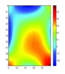
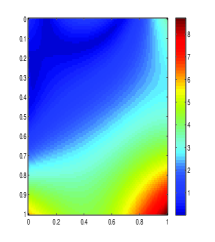
Figure 6.8: (a) expectation of reference state; (b) expectation of state using local-global model reduction method; (c) standard deviations of state obtained by FE method; (d) standard deviations of state using local-global model reduction method.

In Fig. 6.9, we plot the expectation $p_{lg}$ of the boundary control function $g$ using the local-global reduced method. We denote the expectation and standard deviation of reference control by $p_{ref}$ and $\sigma_{ref}$, respectively. We see that the expectation of control variable $g$ using the local-global model reduction method lies in the region between the line $p_{ref}+\sigma_{ref}$ and the line $p_{ref}-\sigma_{ref}$. This shows the credibility of the approximation based on the model reduction.

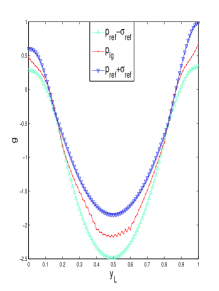
(a) Left boundary

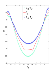
(b) Bottom boundary

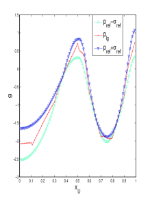
(c) Upper boundary

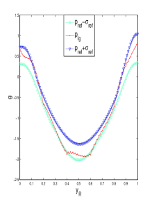
(d) Right boundary

Figure 6.9: Expectation $p$ and standard $\sigma$ of the Neumann boundary condition $g$ on the four boundaries of the domain $\Omega$.

We fix the regularization parameter $\beta$ with $\beta=10^{-4}$ and coarse mesh size with $H=1/5$. For different number of local basis functions at each coarse block and different number of global basis functions, we compute the difference between the state function and target function, and the minimum value of cost functional. The results are listed in Table 7. From the table, we can find that the approximation of the cost functional is not very sensitive to the model fidelity for the boundary control problem.

Table 7: Numerical results with different number of global basis functions $N_{max}$ and different number of local basis functions $L$.

$\sharp~{}of~{}global~{}basis~{}functions$		$L=3$		$L=6$
	$(N_{max})$	$\|u_{lg}(x,\mu)-\hat{u}(x,\mu)\|^{2}_{\mathscr{L}^{2}}$	$J_{min}$	$\|u_{lg}(x,\mu)-\hat{u}(x,\mu)\|^{2}_{\mathscr{L}^{2}}$	$J_{min}$
2		1.099863E-01	5.531052E-02	1.098623E-01	5.524519E-02
4		1.098805E-01	5.525738E-02	1.097684E-01	5.519797E-02

To compare the computation efficiency, we describe the computation setting and list the CPU time in Table 8 when we use the local-global model reduction method and FE method (time in the brackets). By the table, we can find that the local-global model reduction method significantly improves the efficiency compared with standard FE method in fine grid.

Table 8: Comparison of the CPU time for Neumann boundary control problem with FE method and local-global model reduction method.

$\mathbf{Computation~{}setting}$		$\mathbf{Local-global~{}reduced~{}model}$
Number of FE dofs $\mathcal{N}$	10201	Linear system size reduction	1100:1
Number of optimal parameter samples	4	Offline greedy time	2.910E+03 s (3.337E+03 s)
Number of local basis functions	5	Offline time for snapshot spaces	3.997E+02 s (5.397E+01 h)
Number of test parameter samples	2500	Online average time for optimal solutions	1.774E-01 s (1.131 s)

7 Conclusion

In this paper, we have presented a local-global model reduction method for stochastic optimal control problems constrained by PDEs. The possible uncertainty we considered in the paper arises from the PDE coefficient, the target function, the physical domain and the boundary condition. We used reduced basis method and GMsFEM to develop the local-global model reduction. We recast the optimal control problem into a stochastic saddle point formulation and proved the global existence and uniqueness for the stochastic optimal control solution. The local-global model reduction is very suitable for many-query situations. This can significantly enhance the computation efficiency to solve the stochastic optimal control problems. A few numerical examples have been carefully implemented for different stochastic optimal control problems: distributed control on deterministic domain and random domain, boundary control. The numerical results showed the efficacy of the proposed model reduction method and its promising application in stochastic optimal control problems governed by complex models.

References

- [1] M. Alotaibi, V. Calo, Y. Efendiev, J. Galvis and M. Ghommem, Global Clocal nonlinear model reduction for flows in heterogeneous porous media, Comput. Methods Appl. Mech. Engrg., 292 (2015), pp. 122-137.
- [2] I. Babuka, U. Banerjee, J. Osborn, Generalized finite element methods: main ideas, results and perspective, Int. J. Comput. Methods, 1 (2004), pp. 67–103.
- [3] I. Babuka, R. Lipton, Optimal local approximation spaces for generalized finite element methods with application to multiscale problems, Multiscale Model. Simul., 9 (2011), pp. 373–406.
- [4] I. Babuka, J. Osborn, Generalized finite element methods: their performance and their relation to mixed methods, SIAM J. Numer. Anal., 20 (1983), pp. 510–536.
- [5] I. Babuka, R. Tempone, G.E. Zouraris, Galerkin finite element approximations of stochastic elliptic partial differential equations, SIAM J. Numer. Anal., 42 (2004), pp. 800–825.
- [6] M. Barrault, Y. Maday, N. Nguyen, A. Patera, An empirical interpolation method: application to efficient reduced-basis discretization of partial differential equations, C.R. Math. Acad. Sci. Paris, 339 (2004), pp. 667–672.
- [7] P. Bochev, M. Gunzburger, Least-squares finite element methods, volume 166. Springer, New York, 2009.
- [8] F. Brezzi, On the existence, uniqueness and approximation of saddle-point problems arising from Lagrangian multipliers, RAIRO Anal. Num r., 2 (1974), pp, 129–151.
- [9] F. Brezzi, M. Fortin, Mixed and hybrid finite element methods, Springer, New York, 1991.
- [10] A. Buffa, Y. Maday, A. Patera, C. Prudhomme, G. Turinici, A priori convergence of the greedy algorithm for the parametrized reduced basis method, ESAIM Math. Model. Numer. Anal., 46 (2012), pp. 595–603.
- [11] S. Collis, M. Heinkenschloss, Analysis of the streamline upwind/Petrov Galerkin method applied to the solution of optimal control problems, Technical report TR02-01, 2002.
- [12] P. Chen, A. Quarteroni, G. Rozza, Stochastic optimal Robin boundary control problems of advection-dominated elliptic equations, SIAM J. Numer. Anal., 51 (2013), pp. 2700–2722.
- [13] P. Chen, A. Quarteroni, Weighted reduced basis method for stochastic optimal control problems with elliptic PDE constraint, SIAM J. Uncertain. Quantif., 2 (2014), pp. 364–396.
- [14] Y. Chen, J. Hesthaven, Y. Madaym, J. Rodriguez, Certified reduced basis methods and output bounds for the harmonic Maxwels equations, SIAM J. Sci. Comput., 32 (2010), pp. 970–996.
- [15] E. Chung, Y. Efendiev, T. Hou, Adaptive multiscale model reduction with generalized multicale finite element method, SIAM J. Sci. Comput., 320 (2016), pp. 69–95.
- [16] L. Ded, Reduced basis method and a posteriori error estimation for parametrized linear-quadratic optimal control problems, SIAM J. Sci. Comput., 32 (2010), pp. 997–1019.
- [17] Y. Efendiev, J. Galvis, T. Hou, Generalized multiscale finite element methods (GMsFEM), J. Comput. Phys., 251 (2013), pp. 116–135.
- [18] Y. Efendiev, J. Galvis, X. Wu, Multiscale finite element methods for high contrast problems using local spectral basis functions, J. Comput. Phys., 230 (2011), pp. 937–955.
- [19] Y. Efendiev, T. Hou, Multiscale finite element methods: theory and applications, Springer, 2009.
- [20] R. Glowinski, J. Lions, Exact and Approximate Controllability for Distributed Parameter Systems, Cambridge University Press, Cambridge, UK, 1996.
- [21] M. Grepl, M. Karcher, Reduced basis a posteriori error bounds for parametrized linear quadratic elliptic optimal control problems, C. R. Math. Acad. Sci. Paris, 349 (2011), pp. 873–877.
- [22] M. Grepl, Y. Maday, N. Nguyen, A. Patera, Efficient reduced-basis treatment of nonaffine and nonlinear partial differential equations, ESAIM: Model. Math. Anal. Numer., 41 (2007), pp. 575–605.
- [23] M. Gunzburger, H. Lee, J. Lee, Error estimates of stochastic optimal Neumann boundary control problems, SIAM J. Numer. Anal., 49 (2011), pp. 1532–1552.
- [24] L. Hou, J. Lee, H. Manouzi, Finite element approximations of stochastic optimal control problems constrained by stochastic elliptic PDEs, J. Math. Anal. Appl., 384 (2011), pp. 87–103.
- [25] T. Hou, X. Wu, A multiscale finite element method for elliptic problems in composite materials and porous media, J. Comput. Phys., 134 (1997), pp. 169–189.
- [26] D. Huynh, G. Rozza, S. Sen, A. Patera, A successive constraint linear optimization method for lower bounds of parametric coercivity and inf-sup stability constants, C. R. Math. Acad. Sci. Paris, 345 (2007), pp. 473–478.
- [27] L. Jiang, Y. Efendiev, I. Mishev, Mixed multiscale finite element methods using approximate global information based on partial upscaling, Comput. Geosci., 14 (2010), pp. 319–341.
- [28] L. Jiang, Q. Li, Reduced multiscale finite element basis methods for elliptic PDEs with parameterized inputs, J. Comput. Appl. Math. 301 (2016), pp. 101–120.
- [29] L. Jiang, Q. Li, Model’s sparse representation based on reduced mixed GMsFE basis methods, J. Comput. Phys., 338 (2017), pp. 285–312.
- [30] D. Kouri, D. Heinkenschloos, M. Ridzal, et al, A trust-region algorithm with adaptive stochastic collocation for PDE optimization under uncertainty, SIAM J. Sci. Comput., 35 (2013), pp. 1847–1879.
- [31] H. Lee, J. Lee, A stochastic Galerkin method for stochastic control problems, Commun. Comput. Phys., 14 (2013), pp. 77–106.
- [32] J. Lions, Optimal Control of Systems Governed by Partial Differential Equations, Springer, New York, 1971.
- [33] G. Lorentz, M. Golitschek, Y. Makovoz, Constructive Approximation: Advanced Problems, Springer-Verlag, New York, 1996.
- [34] J. Melenk, I. Babuka, The partition of unity finite element method: basic theory and applications, Comput. Methods Appl. Mech. Engrg. 139 (1996), pp. 289–314.
- [35] F. Negri, G. Rozza, A. Manzoni, A. Quarteroni, Reduced basis method for parametrized elliptic optimal control problems, SIAM J. Sci. Comput., 35 (2013), pp. 2316–2340.
- [36] L. Ng and K. Willcox, Multifidelity approaches for optimization under uncertainty, Internat. J. Numer. Methods Engrg., 100 (2014), pp. 746–772.
- [37] J. Pearson, Fast iterative solvers for PDE-constrained optimization problems, University of Oxford, 2013.
- [38] A. Quarteroni, A. Manzoni, F. Negri, Reduced basis methods for partial differential equations, Springer, New York, 2015.
- [39] A. Quarteroni, G. Rozza, A. Manzoni, Certified reduced basis approximation for parametrized partial differential equations and applications, J. Math. Ind., 1 (2011), pp. 1–49.
- [40] T. Rees, H. Dollar, A. Wathen, Optimal solvers for PDE-constrained optimization, SIAM J. Sci. Comput., 32 (2010), pp. 271–298.
- [41] G. Rozza, D. Huynh, A. Patera, Reduced basis approximation and a posteriori error estimation for affinely parametrized elliptic coercive partial differential equations, Arch. Comput. Methods Eng., 15 (2008), pp. 229–275.
- [42] E. Rosseel, G. Wells, Optimal control with stochastic PDE constraints and uncertain controls, Comput. Methods Appl. Mech. Engrg., 213 (2012), pp. 152–167.
- [43] F. Trltzsch, Optimal control of partial differential equations: theory, methods, and applications, AMS, Providence, RI, 2010.
- [44] D. Xiu, D. Tartakovsky Numerical methods for differential equations in random domains, SIAM J. Sci. Comput., 28 (2006), pp. 1167–1185.