Mixing-induced quantum non-Markovianity and information flow

Abstract

Mixing dynamical maps describing open quantum systems can lead from Markovian to non-Markovian processes. Being surprising and counter-intuitive, this result has been used as argument against characterization of non-Markovianity in terms of information exchange. Here, we demonstrate that, quite the contrary, mixing can be understood in a natural way which is fully consistent with existing theories of memory effects. In particular, we show how mixing-induced non-Markovianity can be interpreted in terms of the distinguishability of quantum states, system-environment correlations and the information flow between system and environment.

Introduction. In quantum as well as in classical mechanics the isolation of the system of interest is never perfectly achievable. The effect of external noise or of the interaction with uncontrolled environmental degrees of freedom makes the dynamics stochastic. In quantum mechanics the environmental influence appears as an additional layer of stochasticity, on top of the inherently probabilistic description of any quantum experiment, and cannot be generally described by means of classical stochastic processes. Quantum processes, which can be taken as the description of the evolution of an open quantum system dynamics Breuer and Petruccione (2007), are described by time dependent collections of completely positive trace preserving (CPT) maps, called quantum dynamical maps. The characterization of quantum processes in view of the relationship of these maps at different times, in analogy to the correlations of a classical process at different times, which allow to introduce the very definition of Markovian process, is an important and difficult issue due to the special role of measurement in quantum mechanics.

In recent times a lot of work has been devoted to the study of quantum non-Markovianity (see e.g. Breuer (2012); Rivas et al. (2014); Breuer et al. (2016); de Vega and Alonso (2017)). In particular, a notion of memory for quantum processes has been introduced which can be physically interpreted in terms of the flow of information between the open system and its environment Breuer et al. (2009); Wißmann et al. (2015). The information flow is defined by means of the behavior in time of the distinguishability of two open system states and non-Markovianity is characterized by a non-monotonic time evolution of the distinguishability. Experimental control and measurements of non-Markovian quantum dynamics and of the closely connected impact of initial system-environment correlations have been reported for photonic systems Liu et al. (2011); Li et al. (2011); Tang et al. (2012); Liu et al. (2013); Cialdi et al. (2014); Bernardes et al. (2015); Tang et al. (2015), nuclear magnetic resonance Bernardes et al. (2016), and trapped ion systems Gessner et al. (2014); Wittemer et al. (2017).

However, mixing of quantum dynamical maps leads to new time evolutions, whose Markovianity properties can be related in a quite counter-intuitive way to the Markovianity of the original maps Vacchini (2012); Chruściński and Wudarski (2013, 2015); Wudarski et al. (2015); Kropf et al. (2016); Wudarski and Chruściński (2016). In particular one can consider random mixtures of unitary evolutions showing up memory effects, so that objections have been raised about the validity of the interpretation of non-Markovianity in terms of information flow Pernice et al. (2012); Megier et al. (2017). On the contrary, we show in this contribution by means of a microscopic description that non-Markovianity arising by mixing is naturally understood in terms of information flow. This implies in particular that indeed the collection of quantum dynamical maps giving the reduced system dynamics allows to properly describe memory effects.

Mixing quantum processes. We consider two quantum processes given by one-parameter families of quantum dynamical maps $\Phi^{(1)}_{t}$ and $\Phi^{(2)}_{t}$ with $t\geq 0$. A natural way to construct a new map is to consider the convex linear combination

$$\Phi_{t}=q_{1}\Phi^{(1)}_{t}+q_{2}\Phi^{(2)}_{t},$$ (1)

where $q_{1,2}\geq 0$ and $q_{1}+q_{2}=1$. It is easy to show that $\Phi_{t}$ is, in fact, a CPT map provided that $\Phi^{(1)}_{t}$ and $\Phi^{(2)}_{t}$ are CPT maps. The map $\Phi_{t}$ will be called mixture of the maps $\Phi^{(1)}_{t}$ and $\Phi^{(2)}_{t}$. This construction can be extended to an arbitrary number of dynamical maps $\Phi^{(i)}_{t}$ in an obvious way sup . To keep the notation simple we will restrict here to the case of mixtures of two dynamical maps. A simple but well-known example of this construction is obtained by taking all maps $\Phi^{(i)}_{t}$ to be unitary transformations, in this case the resulting mixture $\Phi_{t}$ is known as random unitary map Landau and Streater (1993); Audenaert and Scheel (2008).

Non-Markovianity. To explain the concept of quantum non-Markovianity to be used in the following Breuer et al. (2009); Wißmann et al. (2015) we consider two parties, Alice and Bob. Alice prepares a quantum system $S$ in one of two states $\rho_{S}^{1}$, $\rho_{S}^{2}$ with probability of $1/2$ each, and then sends the system to Bob. It is Bob’s task to figure out by a single measurement whether the system has been prepared in state $\rho_{S}^{1}$ or $\rho_{S}^{2}$. It can be shown that by an optimal strategy Bob can find the correct state with a maximal success probability given by

$$P_{\max}=\frac{1}{2}\left(1+D(\rho_{S}^{1},\rho_{S}^{2})\right),$$ (2)

where

$$D(\rho_{S}^{1},\rho_{S}^{2})=\frac{1}{2}||\rho_{S}^{1}-\rho_{S}^{2}||$$ (3)

denotes the trace distance of the quantum states. The trace distance thus represents a measure for the distinguishability of quantum states. In these relations it is assumed that Bob receives the quantum system in states $\rho_{S}^{1}$ or $\rho_{S}^{2}$. However, if we assume that Alice prepares her states as states of an open system $S$ which is coupled to some environment $E$, Bob receives instead the states $\rho_{S}^{1}(t)=\Phi_{t}[\rho_{S}^{1}]$ or $\rho_{S}^{2}(t)=\Phi_{t}[\rho_{S}^{2}]$, where $\Phi_{t}$ denotes the quantum dynamical map describing the evolution of $S$. The trace distance of the states available to Bob is then given by $D(\rho_{S}^{1}(t),\rho_{S}^{2}(t))$ and, hence, the maximal probability with which he can correctly identify the state is given by

$$P^{\Phi}_{\max}(t)=\frac{1}{2}\left(1+\frac{1}{2}||\Phi_{t}[\rho_{S}^{1}-\rho_{S}^{2}]||\right).$$ (4)

A quantum process given in terms of a family of quantum dynamical maps $\Phi_{t}$ is defined to be Markovian if the trace distance $D(\rho_{S}^{1}(t),\rho_{S}^{2}(t))$ is a monotonically decreasing function of time $t$ for all pairs of initial states. Hence, quantum non-Markovianity is characterized by a temporal increase of the trace distance for a certain pair of initial states. Since the trace distance represents a measure for the distinguishability of quantum states, a decrease of the trace distance can be interpreted as a loss of information from the open system $S$ into the environment $E$. Correspondingly, any increase of the trace distance corresponds to a flow of information from the environment back to the open system which is characteristic of the presence of memory effects. On the basis of these concepts one can also define a measure for the degree of non-Markovianity by means of

$$\mathcal{N}(\Phi)=\max_{\rho^{1,2}_{S}}\int_{\sigma>0}dt\;\sigma(t),$$ (5)

where

$$\sigma(t)\equiv\frac{d}{dt}D\left(\Phi_{t}\rho^{1}_{S},\Phi_{t}\rho^{2}_{S}\right).$$ (6)

Thus, $\mathcal{N}(\Phi)$ quantifies the amount of the total information which flows back from the environment into the open system during the time evolution.

How does this concept of memory effects in quantum mechanics and the associated measure of non-Markovianity behave under mixing of quantum dynamical maps? It is quite natural to expect that mixing always makes quantum processes more Markovian. According to several examples constructed in the literature Chruściński and Wudarski (2015); Kropf et al. (2016) this intuitive expectation is false. Indeed, it is even possible that $\Phi_{t}$ is non-Markovian although the dynamical maps $\Phi^{(i)}_{t}$ are Markovian, and even represent quantum dynamical semigroups sup . Thus, the set of Markovian processes is not convex and the following questions arise: How can memory effects emerge through the simple process of mixing quantum processes, and how can this be interpreted in terms of a backflow of information from the environment to the open system? To discuss these issues we first design an appropriate microscopic description for the mixing procedure.

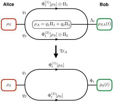
Figure 1: Scheme of the microscopic interaction leading to the maps $\Lambda_{t}$ and $\Phi_{t}$. In both cases the system state is coupled to two environments and an ancilla in a fixed state. The map $\Lambda_{t}$ describes the state of both system and ancilla at time $t$, while $\Phi_{t}$ provides the transformed state of the system only.

Microscopic representation of mixing. We start from the following representations for the dynamical maps $\Phi^{(1)}_{t}$ and $\Phi^{(2)}_{t}$:

$$\Phi^{(i)}_{t}[\rho_{S}]={\mathrm{Tr}}_{E_{i}}\Big{[}U^{(i)}_{t}\rho_{S}\otimes\rho_{E_{i}}U^{(i)\dagger}_{t}\Big{]},\quad i=1,2.$$ (7)

These maps act on the density matrices $\rho_{S}$ of the state space of the open system which we denote by $\mathcal{S}(\mathcal{H}_{S})$, where $\mathcal{H}_{S}$ is the underlying Hilbert space. For each $i$, $\rho_{E_{i}}$ is a fixed environmental state taken from the state space $\mathcal{S}(\mathcal{H}_{E_{i}})$ of environment $E_{i}$, and the unitary time-evolution operator $U^{(i)}_{t}$ is taken to be

$$U^{(i)}_{t}=\exp(-iH_{i}t),$$ (8)

where $H_{i}$ is the Hamiltonian for the composite system $S+E_{i}$ with Hilbert space $\mathcal{H}_{S}\otimes\mathcal{H}_{E_{i}}$. For simplicity we assume the Hamiltonians to be time-independent. The generalization to time-dependent Hamiltonians is straightforward. Finally, ${\mathrm{Tr}}_{E_{i}}$ denotes the partial trace over environment $E_{i}$.

Our goal is to develop a microscopic representation of the time evolution corresponding to the convex linear combination (1). To this end, we couple our open system $S$ to the two different environments $E_{1}$, $E_{2}$ and, additionally, to an ancilla system $A$ with a two-dimensional Hilbert space $\mathcal{H}_{A}$. The Hilbert space of the total system is thus given by $\mathcal{H}_{S}\otimes\mathcal{H}_{E_{1}}\otimes\mathcal{H}_{E_{2}}\otimes\mathcal{H}_{A}$, and the total system Hamiltonian is taken to be

$$H=H_{1}\otimes\Pi_{1}+H_{2}\otimes\Pi_{2}.$$ (9)

Here, $H_{i}$ describes, as above, the coupling between the open system $S$ and environment $E_{i}$, while $\Pi_{i}=|i\rangle\langle i|$ are orthogonal rank-one projections corresponding to some basis $|i\rangle$, $i=1,2$, of the ancilla Hilbert space $\mathcal{H}_{A}$. Taking as initial state of the ancilla system the fixed state

$$\rho_{A}=q_{1}\Pi_{1}+q_{2}\Pi_{2},$$ (10)

one can introduce a microscopic representation for the mixture of dynamical maps Eq. (1) which is illustrated in Fig. 1. Indeed, denoting by $U_{t}=\exp(-iHt)$ the unitary time-evolution operator of the total system, one can consider the map

$$\Lambda_{t}[\rho_{S}]={\mathrm{Tr}}_{E_{1}}{\mathrm{Tr}}_{E_{2}}\big{[}U_{t}\rho_{S}\otimes\rho_{E_{1}}\otimes\rho_{E_{2}}\otimes\rho_{A}U^{\dagger}_{t}\big{]},$$ (11)

which can be written as sup

$$\Lambda_{t}[\rho_{S}]=q_{1}\Phi^{(1)}_{t}[\rho_{S}]\otimes\Pi_{1}+q_{2}\Phi^{(2)}_{t}[\rho_{S}]\otimes\Pi_{2}.$$ (12)

Taking the partial trace with respect to the ancilla degrees of freedom one obtains from this equation sup

$$\Phi_{t}[\rho_{S}]={\mathrm{Tr}}_{E_{1}}{\mathrm{Tr}}_{E_{2}}{\mathrm{Tr}}_{A}\big{[}U_{t}\rho_{S}\otimes\rho_{E_{1}}\otimes\rho_{E_{2}}\otimes\rho_{A}U^{\dagger}_{t}\big{]}.$$ (13)

Thus, we have shown that any mixture of quantum dynamical maps of the form of Eq. (1) admits a microscopic representation of the form (13) with the help of an additional ancilla qubit system. To explain the physical interpretation of this construction we consider again the two parties Alice and Bob. Alice prepares the quantum system $S$ in a certain state $\rho_{S}$ and sends it to Bob through quantum channels $\Phi^{(i)}_{t}$ with respective probabilities $q_{i}$. Thus, Bob receives the states $\Phi^{(i)}_{t}[\rho_{S}]$ with corresponding probability $q_{i}$.

Let us suppose first that Bob has access not only to the degrees of freedom of $S$, but also to the degrees of freedom of the ancilla system $A$. Bob can then obviously figure out which channel has acted on the input state $\rho_{S}$. This is due to the correlations in the system-ancilla state $\Lambda_{t}[\rho_{S}]$ shown in Eq. (12). In fact, if Bob measures, for example, $\Pi_{1}$ he will find $\Pi_{1}=1$ with probability $q_{1}$ and in this case he knows that the channel $\Phi^{(1)}_{t}[\rho_{S}]$ has acted on the input state. Accordingly, he will get the outcome $\Pi_{1}=0$ with probability $q_{2}$ in which case he knows that the channel $\Phi^{(2)}_{t}[\rho_{S}]$ has acted on the input state. Hence, the map $\Lambda_{t}$ describes the situation in which Bob does know the channel which has acted on the input state. Note that the ancilla represents, essentially, a classical degree of freedom which does not change in time because of ${\mathrm{Tr}}_{S}\Lambda_{t}[\rho_{S}]=\rho_{A}$, and that the correlations between system and ancilla are purely classical correlations (no entanglement and zero quantum discord).

Hence, if Bob has access to the ancilla degree of freedom (see Fig. 2) the maximal success probability with which he can correctly identify the state is given by

$$p^{\Lambda}_{\textrm{max}}(t)=q_{1}p^{\Phi^{(1)}}_{\textrm{max}}(t)+q_{2}p^{\Phi^{(2)}}_{\textrm{max}}(t).$$ (14)

Employing expression (4) and the general relation sup

$$||\Lambda_{t}[X]||=q_{1}||\Phi^{(1)}_{t}[X]||+q_{2}||\Phi^{(2)}_{t}[X]||$$ (15)

we obtain

$$p^{\Lambda}_{\textrm{max}}(t)=\frac{1}{2}\left(1+\frac{1}{2}||\Lambda_{t}[\rho_{S}^{1}-\rho_{S}^{2}]||\right).$$ (16)

Thus we see that the distinguishability under $\Lambda_{t}$ is equal to the weighted sum of the distinguishabilities under $\Phi_{t}^{(1)}$ and $\Phi_{t}^{(2)}$. Therefore, if $\Phi_{t}^{(1)}$ and $\Phi_{t}^{(2)}$ are Markovian, then $\Lambda_{t}$ is also Markovian. On the other hand, if $\Phi_{t}^{(1)}$ or $\Phi_{t}^{(2)}$ is non-Markovian, then $\Lambda_{t}$ can be Markovian or non-Markovian, depending on whether or not the increase of the trace distance under e.g. $\Phi_{t}^{(1)}$ is compensated by a corresponding decrease of the trace distance under $\Phi_{t}^{(2)}$. In this sense on can say that, in general, $\Lambda_{t}$ is more Markovian than $\Phi_{t}^{(1)}$ and $\Phi_{t}^{(2)}$. Formally, this result can be expressed by the general relation sup

$$\mathcal{N}(\Lambda)\leq q_{1}\mathcal{N}(\Phi^{(1)})+q_{2}\mathcal{N}(\Phi^{(2)}).$$ (17)

Figure 2: Given a pair of initial states $\rho_{S}^{1,2}$ prepared by Alice, Bob has two different optimal measurement strategies to discriminate between them for the two maps $\Lambda_{t}$ and $\Phi_{t}$. In particular $P^{\Lambda}_{\max}(t)\geq P^{\Phi}_{\max}(t)$ since in the first case Bob can also access the degrees of freedom of the ancilla.

Non-Markovianity induced by mixing. Let us now suppose that Bob has no access to the ancilla degrees of freedom and, hence, has no information about whether the channel $\Phi^{(1)}_{t}$ or $\Phi^{(2)}_{t}$ has been used by Alice. Bob only knows the corresponding probabilities $q_{1}$ and $q_{2}$. In this situation he has to describe the channel by the convex linear combination (1) since the states he receives are the statistical mixtures $q_{1}\Phi^{(1)}_{t}[\rho_{S}]+q_{2}\Phi^{(2)}_{t}[\rho_{S}]$. It follows that the maximal probability for correct state identification by Bob is now given by

$$P^{\Phi}_{\max}(t)=\frac{1}{2}\left(1+\frac{1}{2}||\Phi_{t}[\rho_{S}^{1}-\rho_{S}^{2}]||\right).$$ (18)

Using $\Phi_{t}=\mathrm{Tr}_{A}\circ\Lambda_{t}$ as well as the fact that the trace operation is a contraction under the trace norm Ruskai (1994), we immediately obtain (see also Fig. 2)

$$P^{\Phi}_{\max}(t)\leq P^{\Lambda}_{\max}(t)=q_{1}P^{\Phi^{(1)}}_{\max}(t)+q_{2}P^{\Phi^{(2)}}_{\max}(t).$$ (19)

According to this inequality the process $\Phi_{t}$, in contrast to the process $\Lambda_{t}$ acting on both system and ancilla degree of freedom, can be non-Markovian even though both $\Phi^{(1)}_{t}$ and $\Phi^{(2)}_{t}$ are Markovian. In fact, the inequality gives room for the trace distance under $\Phi_{t}$ to behave non-monotonically although the trace distances under $\Phi^{(1)}_{t}$ and $\Phi^{(2)}_{t}$ are monotonically decreasing corresponding to Markovian dynamics. The reason for this is obviously the partial trace over the ancilla, which leads to a loss of information about the channel acting on the system states. Hence, in the case of non-Markovian dynamics of $\Phi_{t}$ with $\Phi^{(1)}_{t}$ and $\Phi^{(2)}_{t}$ Markovian the interpretation is that there is a backflow of information from the ancilla $A$ to the open system $S$.

Information backflow analysis. This idea of information backflow from the ancilla to the system can be made more precise as follows. We define the quantities

$$I_{\mathrm{int}}(t) = \frac{1}{2}||\Phi_{t}[\rho_{S}^{1}-\rho_{S}^{2}]||,$$ (20)

$$I_{\mathrm{ext}}(t) = \frac{1}{2}||\Lambda_{t}[\rho_{S}^{1}-\rho_{S}^{2}]||-\frac{1}{2}||\Phi_{t}[\rho_{S}^{1}-\rho_{S}^{2}]||.$$ (21)

The quantity $I_{\mathrm{int}}(t)$ is the distinguishability in the case that Bob has no access to the ancilla degrees of freedom. This quantity may thus be interpreted as the internal information, i.e. as the information available if only access to the open system $S$ is possible. On the other hand, the quantity $I_{\mathrm{ext}}(t)$ is the distinguishability including the ancilla degrees of freedom minus the distinguishability without ancilla. Hence, we can interpret $I_{\mathrm{ext}}(t)$ as external information, i.e. as the information which is gained if one includes the ancilla degrees of freedom. Note that $I_{\mathrm{ext}}(t)\geq 0$ and that $\Lambda_{t=0}[\rho_{S}]=\rho_{S}\otimes\rho_{A}$ from which it follows that $I_{\mathrm{ext}}(0)=0$. Moreover, we have $\mathrm{Tr}_{A}\Lambda_{t}[\rho_{S}]=\Phi_{t}[\rho_{S}]$ and $\mathrm{Tr}_{S}\Lambda_{t}[\rho_{S}]=\rho_{A}$ which shows that $\Phi_{t}[\rho_{S}]\otimes\rho_{A}$ is the product of the marginals of the state $\Lambda_{t}[\rho_{S}]$. Now, one can prove the inequality sup ,

$$I_{\mathrm{ext}}(t)\leq D(\Lambda_{t}[\rho_{S}^{1}],\Phi_{t}[\rho_{S}^{1}]\otimes\rho_{A})+D(\Lambda_{t}[\rho_{S}^{2}],\Phi_{t}[\rho_{S}^{2}]\otimes\rho_{A}),$$ (22)

where the quantity $D(\Lambda_{t}[\rho_{S}],\Phi_{t}[\rho_{S}]\otimes\rho_{A})$, representing the trace distance between the state $\Lambda_{t}[\rho_{S}]$ and the product of its marginals, provides a measure for the system-ancilla correlations in the state $\Lambda_{t}[\rho_{S}]$. We recall that these correlations are of purely classical nature.

The inequality (22) shows that the external information is bounded from above by the sum of the correlation measures of the states $\Lambda_{t}[\rho_{S}^{1}]$ and $\Lambda_{t}[\rho_{S}^{2}]$. In particular, when $I_{\mathrm{ext}}(t)$ starts to increase over the initial value $I_{\mathrm{ext}}(0)=0$ correlations between the open system and the ancilla are created. In other words, any nonzero external information implies that there are system-ancilla correlations which are inaccessible to Bob if he can only measure the observables of the open system $S$.

For the interesting special case referred to above, namely that $\Phi^{(1)}_{t}$ and $\Phi^{(2)}_{t}$ are Markovian while the convex mixture $\Phi_{t}$ is non-Markovian, the trace distance $\frac{1}{2}||\Lambda_{t}[\rho_{S}^{1}-\rho_{S}^{2}]||$ decreases monotonically, so that we have

$$\dot{I}_{\mathrm{int}}(t)+\dot{I}_{\mathrm{ext}}(t)\leq 0.$$ (23)

However, the quantity $I_{\mathrm{int}}(t)=\frac{1}{2}||\Phi_{t}[\rho_{S}^{1}-\rho_{S}^{2}]||$ must be a non-monotonic function of time $t$ for a certain pair of initial states $\rho_{S}^{1,2}$. Hence, it follows that $\dot{I}_{\mathrm{int}}(t)>0$ for certain times $t$ which implies $\dot{I}_{\mathrm{ext}}(t)<0$, i.e. there is a nonzero backflow of information from the ancilla into the open system. This clearly supports our interpretation of mixing-induced non-Markovianity. We note that for $\dot{I}_{\mathrm{int}}(t)<0$ we cannot generally draw any conclusion about the sign of the external information $\dot{I}_{\mathrm{ext}}(t)$ from inequality (23). This is due to the fact that the open system can lose information both to the ancilla and to the environments $E_{i}$. Finally, we consider the particularly relevant case of a random mixture of unitary maps. In this case the trace distance $\frac{1}{2}||\Lambda_{t}[\rho_{S}^{1}-\rho_{S}^{2}]||$ is constant in time and, hence, the inequality of Eq. (23) actually becomes an equality, corresponding to the fact that now the system can lose information only to the ancilla.

Conclusions. We have constructed a microscopic representation for a quantum dynamical map arising as a convex mixture of dynamical maps. Our construction allows to understand the relationship between the Markovianity of the quantum dynamical map obtained by mixing and the Markovianity of the single elements of the mixture. The analysis shows in particular that counterintuitive behaviours, such as the emergence of non-Markovianity by mixing Markovian semigroups or unitary dynamics, can be clearly explained and understood within a consistent characterization of non-Markovianity in terms of the flow of information between the open system and its environment.

The crucial point of our construction is the fact that the operation of mixing involves an ancilla system which behaves essentially as a classical degree of freedom, acting as a random number generator which determines the choice of the quantum channel. It therefore plays a similar role as the classical device considered in the seminal work on quantum correlations Werner (1989). While the reduced state of the ancilla does not change in time, correlation between the open system and the ancilla are built up during the time evolution. Thus, the open system can exchange information with the ancilla degree of freedom by virtue of these correlations, and it is this exchange of information which leads to mixing-induced quantum non-Markovianity. These results clearly reinforce the physical motivation underlying the description of quantum memory in terms of distinguishability of quantum states, system-environment correlations and information flow between system and environment.

Appendix A Proofs

A.1 Proof of Eqs. (12) and (13)

In order to prove Eq. (12) of the main text we start from the definition

$$\Lambda_{t}[\rho_{S}]={\mathrm{Tr}}_{E_{1}}{\mathrm{Tr}}_{E_{2}}\big{[}U_{t}\rho_{S}\otimes\rho_{E_{1}}\otimes\rho_{E_{2}}\otimes\rho_{A}U^{\dagger}_{t}\big{]}.$$ (24)

Note that this is a CPT map

$$\Lambda_{t}:\mathcal{S}(\mathcal{H}_{S})\rightarrow\mathcal{S}(\mathcal{H}_{S}\otimes\mathcal{H}_{A}).$$ (25)

Since $\Pi_{1}\Pi_{2}=0$ we can split the unitary time-evolution operator as

$$U_{t}=e^{-iHt}=e^{-iH_{1}\Pi_{1}t}e^{-iH_{2}\Pi_{2}t}.$$ (26)

Using also Eq. (10) of the main text we find

$$\Lambda_{t}[\rho_{S}] = \textrm{ }q_{1}{\mathrm{Tr}}_{E_{1}}{\mathrm{Tr}}_{E_{2}}\big{[}U_{t}\rho_{S}\otimes\rho_{E_{1}}\otimes\rho_{E_{2}}\otimes\Pi_{1}U^{\dagger}_{t}\big{]}$$ (27)

$$+\textrm{ }q_{2}{\mathrm{Tr}}_{E_{1}}{\mathrm{Tr}}_{E_{2}}\big{[}U_{t}\rho_{S}\otimes\rho_{E_{1}}\otimes\rho_{E_{2}}\otimes\Pi_{2}U^{\dagger}_{t}\big{]}$$

$$= \textrm{ }q_{1}{\mathrm{Tr}}_{E_{1}}{\mathrm{Tr}}_{E_{2}}\big{[}U^{(1)}_{t}\rho_{S}\otimes\rho_{E_{1}}\otimes\rho_{E_{2}}\otimes\Pi_{1}U^{(1)\dagger}_{t}\big{]}$$

$$+\textrm{ }q_{2}{\mathrm{Tr}}_{E_{1}}{\mathrm{Tr}}_{E_{2}}\big{[}U^{(2)}_{t}\rho_{S}\otimes\rho_{E_{1}}\otimes\rho_{E_{2}}\otimes\Pi_{2}U^{(2)\dagger}_{t}\big{]}$$

$$= \textrm{ }q_{1}{\mathrm{Tr}}_{E_{1}}\big{[}U^{(1)}_{t}\rho_{S}\otimes\rho_{E_{1}}U^{(1)\dagger}_{t}\big{]}\otimes\Pi_{1}$$

$$+\textrm{ }q_{2}{\mathrm{Tr}}_{E_{2}}\big{[}U^{(2)}_{t}\rho_{S}\otimes\rho_{E_{2}}U^{(2)\dagger}_{t}\big{]}\otimes\Pi_{2}.$$

Employing Eq. (7) of the main text we can rewrite this as

$$\Lambda_{t}[\rho_{S}]=q_{1}\Phi^{(1)}_{t}[\rho_{S}]\otimes\Pi_{1}+q_{2}\Phi^{(2)}_{t}[\rho_{S}]\otimes\Pi_{2}$$ (28)

which proves Eq. (12) of the main text. Tracing over the ancilla degree of freedom we find

$${\mathrm{Tr}}_{A}\Lambda_{t}[\rho_{S}] = q_{1}\Phi^{(1)}_{t}[\rho_{S}]+q_{2}\Phi^{(2)}_{t}[\rho_{S}]$$

$$= \Phi_{t}[\rho_{S}]$$

$$= {\mathrm{Tr}}_{E_{1}}{\mathrm{Tr}}_{E_{2}}{\mathrm{Tr}}_{A}\big{[}U_{t}\rho_{S}\otimes\rho_{E_{1}}\otimes\rho_{E_{2}}\otimes\rho_{A}U^{\dagger}_{t}\big{]},$$

which proves Eq. (13) of the main text.

A.2 Proof of Eq. (15)

To prove Eq. (15) of the main text we start from

$$\Lambda_{t}[X]=q_{1}\Phi^{(1)}_{t}[X]\otimes\Pi_{1}+q_{2}\Phi^{(2)}_{t}[X]\otimes\Pi_{2},$$ (30)

where $X$ is any system operator. Note that the operators $\Phi^{(1)}_{t}[X]\otimes\Pi_{1}$ and $\Phi^{(2)}_{t}[X]\otimes\Pi_{2}$ have orthogonal support in $\mathcal{H}_{S}\otimes\mathcal{H}_{A}$ and, hence, we have

$$||\Lambda_{t}[X]||=q_{1}||\Phi^{(1)}_{t}[X]\otimes\Pi_{1}||+q_{2}||\Phi^{(2)}_{t}[X]\otimes\Pi_{2}||.$$ (31)

Using $||A\otimes B||=||A||\cdot||B||$ and $||\Pi_{1,2}||=1$ we obtain Eq. (15) of the main text.

A.3 Proof of Eq. (17)

To prove Eq. (17) of the main text we use the definition of the non-Markovianity measure for the map $\Lambda_{t}$:

$${\mathcal{N}}(\Lambda)=\max_{\rho_{S}^{1,2}}\int_{\sigma_{\Lambda}>0}dt\;\sigma_{\Lambda}(t),$$ (32)

where

$$\sigma_{\Lambda}(t)\equiv\frac{1}{2}\frac{d}{dt}||\Lambda_{t}[\rho_{S}^{1}-\rho_{S}^{2}]||.$$ (33)

Let $\rho_{S}^{1,2}$ be an optimal state pair for which the maximum in Eq. (32) is attained. Then we can write

$${\mathcal{N}}(\Lambda)=\int_{\sigma_{\Lambda}>0}dt\;\sigma_{\Lambda}(t).$$ (34)

Using Eq. (15) of the main text we get

$$\sigma_{\Lambda}(t)=q_{1}\sigma_{1}(t)+q_{2}\sigma_{2}(t),$$ (35)

where

$$\sigma_{i}(t)\equiv\frac{1}{2}\frac{d}{dt}||\Phi^{(i)}_{t}[\rho_{S}^{1}-\rho_{S}^{2}]||.$$ (36)

Thus, we find

$${\mathcal{N}}(\Lambda)=q_{1}\int_{\sigma_{\Lambda}>0}dt\;\sigma_{1}(t)+q_{2}\int_{\sigma_{\Lambda}>0}dt\;\sigma_{2}(t).$$ (37)

Now, we have

$$\int_{\sigma_{\Lambda}>0}dt\;\sigma_{1}(t)\leq\int_{\sigma_{1}>0}dt\;\sigma_{1}(t).$$ (38)

This is due to the fact that the integration on the right-hand side is extended over all regions in which the function $\sigma_{1}(t)$ is positive and, hence, the integral on the right-hand side is larger or equal to the integral of $\sigma_{1}(t)$ over any other region, in particular over the region given by $\sigma_{\Lambda}(t)>0$. Moreover, we obtain directly from the definition of quantum non-Markovianity that

$$\int_{\sigma_{1}>0}dt\;\sigma_{1}(t)\leq{\mathcal{N}}(\Phi^{(1)}).$$ (39)

Together with (38) this yields

$$\int_{\sigma_{\Lambda}>0}dt\;\sigma_{1}(t)\leq{\mathcal{N}}(\Phi^{(1)}).$$ (40)

In the same manner we obtain

$$\int_{\sigma_{\Lambda}>0}dt\;\sigma_{2}(t)\leq{\mathcal{N}}(\Phi^{(2)}).$$ (41)

Using Eqs. (40) and (41) in Eq. (37) we finally get the desired result:

$$\mathcal{N}(\Lambda)\leq q_{1}\mathcal{N}(\Phi^{(1)})+q_{2}\mathcal{N}(\Phi^{(2)}).$$ (42)

A.4 Proof of Eq. (22)

To prove Eq. (22) of the main text we start from the definition

$$I_{\textrm{ext}}(t)=\frac{1}{2}||\Lambda_{t}[\rho_{S}^{1}-\rho_{S}^{2}]||-\frac{1}{2}||\Phi_{t}[\rho_{S}^{1}-\rho_{S}^{2}]||.$$ (43)

Since $\rho_{A}\in\mathcal{S}(\mathcal{H}_{A})$ has unit trace norm we have

$$||\Phi_{t}[\rho_{S}^{1}-\rho_{S}^{2}]||=||\Phi_{t}[\rho_{S}^{1}-\rho_{S}^{2}]\otimes\rho_{A}||.$$ (44)

Using the triangular inequality for the trace norm,

$$\Big{|}||A||-||B||\Big{|}\leq||A-B||,$$ (45)

we obtain

$$I_{\textrm{ext}}(t) \leq \frac{1}{2}||\Lambda_{t}[\rho_{S}^{1}-\rho_{S}^{2}]-\Phi_{t}[\rho_{S}^{1}-\rho_{S}^{2}]\otimes\rho_{A}||$$ (46)

$$= \frac{1}{2}||(\Lambda_{t}[\rho_{S}^{1}]-\Phi_{t}[\rho_{S}^{1}]\otimes\rho_{A})$$

$$\quad-(\Lambda_{t}[\rho_{S}^{2}]-\Phi_{t}[\rho_{S}^{2}]\otimes\rho_{A})||.$$

Employing the triangular inequality

$$||A-B||\leq||A||+||B||$$ (47)

we finally get Eq. (22) of the main text:

$$I_{\textrm{ext}}(t) \leq \frac{1}{2}||\Lambda_{t}[\rho_{S}^{1}]-\Phi_{t}[\rho_{S}^{1}]\otimes\rho_{A}||$$ (48)

$$+\frac{1}{2}||\Lambda_{t}[\rho_{S}^{2}]-\Phi_{t}[\rho_{S}^{2}]\otimes\rho_{A}||.$$

Appendix B MIXING QUANTUM PROCESSES

For simplicity, the presentation of the main text has been restricted to the mixing of two dynamical maps. Our results can easily be generalized to an arbitrary number $n$ of dynamical maps $\Phi_{t}^{(i)}$, where $i=1,2,\ldots,n$. The convex mixture of such maps is defined by

$$\Phi_{t}=\sum_{i=1}^{n}q_{i}\Phi^{(i)}_{t},$$ (49)

where $q_{i}$ is a probability distribution, i.e. $q_{i}\geq 0$ and $\sum_{i}q_{i}=1$. In order to construct the corresponding microscopic representation we take an ancilla $A$ with $n$-dimensional Hilbert space $\mathcal{H}_{A}$. Introducing an orthonormal basis $|i\rangle$ in this space we define rank-one projection operators $\Pi_{i}=|i\rangle\langle i|$ and a fixed initial state of the ancilla system

$$\rho_{A}=\sum_{i=1}^{n}q_{i}\Pi_{i}.$$ (50)

The Hamiltonian of the total system is taken to be

$$H=\sum_{i=1}^{n}H_{i}\otimes\Pi_{i},$$ (51)

where $H_{i}$ describes the interaction of the open system $S$ with environment $E_{i}$. The time evolution operator factorizes,

$$U_{t}=\exp(-iHt)=\prod_{i=1}^{n}\exp(-iH_{i}\Pi_{i}t),$$ (52)

because of $\Pi_{i}\Pi_{j}=\delta_{ij}\Pi_{i}$. The map defined by

$$\Lambda_{t}[\rho_{S}]={\mathrm{Tr}}_{E_{1}}...{\mathrm{Tr}}_{E_{n}}\Big{[}U_{t}\rho_{S}\otimes\rho_{E_{1}}\otimes\ldots\otimes\rho_{E_{n}}\otimes\rho_{A}U^{\dagger}_{t}\Big{]}$$ (53)

can thus be written as

$$\Lambda_{t}[\rho_{S}]=\sum_{i=1}^{n}q_{i}\Phi^{(i)}_{t}[\rho_{S}]\otimes\Pi_{i}.$$ (54)

Taking the partial trace over the ancilla degrees of freedom we find

$${\mathrm{Tr}}_{A}\Lambda_{t}[\rho_{S}] = \sum_{i=1}^{n}q_{i}\Phi^{(i)}_{t}[\rho_{S}]$$

$$= \Phi_{t}[\rho_{S}]$$

$$= {\mathrm{Tr}}_{E_{1}}...{\mathrm{Tr}}_{E_{n}}{\mathrm{Tr}}_{A}\Big{[}U_{t}\rho_{S}\otimes\rho_{E_{1}}\ldots\rho_{E_{n}}\otimes\rho_{A}U^{\dagger}_{t}\Big{]}$$

which is the desired microscopic representation of the mixture $\Phi_{t}$ analogous to Eq. (13) of the main text.

Appendix C GENERALIZED NON-MARKOVIANITY

In the main text we have used the concept of quantum non-Markovianity based on the trace distance which represents a measure for the distinguishability of quantum states $\rho_{S}^{1}$ and $\rho_{S}^{2}$ prepared with equal probabilities of $1/2$. Recently, this concept of non-Markovianity has been extended to include the case that $\rho_{S}^{1}$ and $\rho_{S}^{2}$ are prepared with different probabilities $p_{1}$ and $p_{2}$ Wißmann et al. (2015); Breuer et al. (2016). It can be shown that by an optimal strategy Bob can now distinguish the states with a maximal probability given by

$$P_{\textrm{max}}^{\Phi}(t)=\frac{1}{2}\left(1+||\Phi_{t}[\Delta]||\right),$$ (56)

where

$$\Delta=p_{1}\rho_{S}^{1}-p_{2}\rho_{S}^{2}$$ (57)

is the Helstrom matrix Helstrom (1976). Consequently, the generalized measure of non-Markovianity is defined by means of

$$\tilde{\mathcal{N}}(\Phi)=\max_{p_{i},\rho^{i}_{S}}\int_{\tilde{\sigma}>0}dt\;\tilde{\sigma}(t),$$ (58)

where

$$\tilde{\sigma}(t)\equiv\frac{d}{dt}||\Phi_{t}[\Delta]||.$$ (59)

The discussion presented in the main text can be generalized straightforwardly to this more general notion of quantum non-Markovianity. For example, it can be shown that Eq. (17) of the main text becomes

$$\tilde{\mathcal{N}}(\Lambda)\leq q_{1}\tilde{\mathcal{N}}(\Phi^{(1)})+q_{2}\tilde{\mathcal{N}}(\Phi^{(2)}),$$ (60)

while Eq. (22) of the main text now takes the form

$$I_{\mathrm{ext}}(t) \leq p_{1}||\Lambda_{t}[\rho_{S}^{1}]-\Phi_{t}[\rho_{S}^{1}]\otimes\rho_{A}||$$ (61)

$$+p_{2}||\Lambda_{t}[\rho_{S}^{2}]-\Phi_{t}[\rho_{S}^{2}]\otimes\rho_{A}||,$$

where $I_{\textrm{ext}}(t)\equiv||\Lambda_{t}[\Delta]||-||\Phi_{t}[\Delta]||$.

Appendix D EXAMPLES

D.1 Non-Markovian mixtures of semigroups

For a qubit system consider for $k=1,2$ the maps

$$\Phi^{(k)}_{t}[\rho_{S}]=\mu_{k}(t)\rho_{S}+(1-\mu_{k}(t))\sum_{j=0,1}Q_{j}\rho_{S}Q_{j},$$ (62)

where $Q_{j}=|j\rangle\langle j|$ are the projections onto the eigenstates of the operator $\sigma_{z}$ for the system and the complex coefficients $\mu_{k}(t)$ are given by

$$\mu_{k}(t)=e^{-(\gamma_{k}+i\lambda_{k})t}.$$ (63)

These maps describe pure dephasing of the qubit, obeying a Markovian semigroup dynamics with Hamiltonian contribution $({\lambda_{k}}/{2})\sigma_{z}$, and a single Lindblad operator $\sigma_{z}$ with corresponding rate $\gamma_{k}$. Considering a convex mixture of $\Phi^{(1)}_{t}$ and $\Phi^{(2)}_{t}$ as in Eq. (1) of the main text one has that coherences evolve as

$$\langle 1|\rho_{S}(t)|0\rangle=\mathsf{k}(t)\langle 1|\rho_{S}|0\rangle,$$ (64)

where

$$\mathsf{k}(t)=q_{1}\mu_{1}(t)+q_{2}\mu_{2}(t).$$ (65)

The distinguishability of an optimal pair of states (a pair of states for which the maximum in Eq. (5) of the main text is attained) is given by the modulus of $\mathsf{k}(t)$,

$$|\mathsf{k}(t)|$$

$$= \sqrt{q_{1}^{2}e^{-2\gamma_{1}t}+q_{2}^{2}e^{-2\gamma_{2}t}+2q_{1}q_{2}e^{-(\gamma_{1}+\gamma_{2})t}\cos(\Delta_{\lambda}t)}.$$

For the case $\Delta_{\lambda}\!=\!\lambda_{2}-\lambda_{1}\not=0$ this distinguishability can indeed exhibit a non-monotonic behavior, corresponding to a backflow of information, even though both $\Phi^{(1)}_{t}$ and $\Phi^{(2)}_{t}$ describe a Markovian dynamics. Examples are shown in Fig. 3 and Fig. 4. Note in particular that for the special case $\gamma_{1}=\gamma_{2}=0$ one recovers an example of random unitary map.

Figure 3: The distinguishability (LABEL:eq:osckappa) of optimal state pairs as a function of time. In these graphs $\lambda_{1}=2\pi$ and $\lambda_{2}=0$.

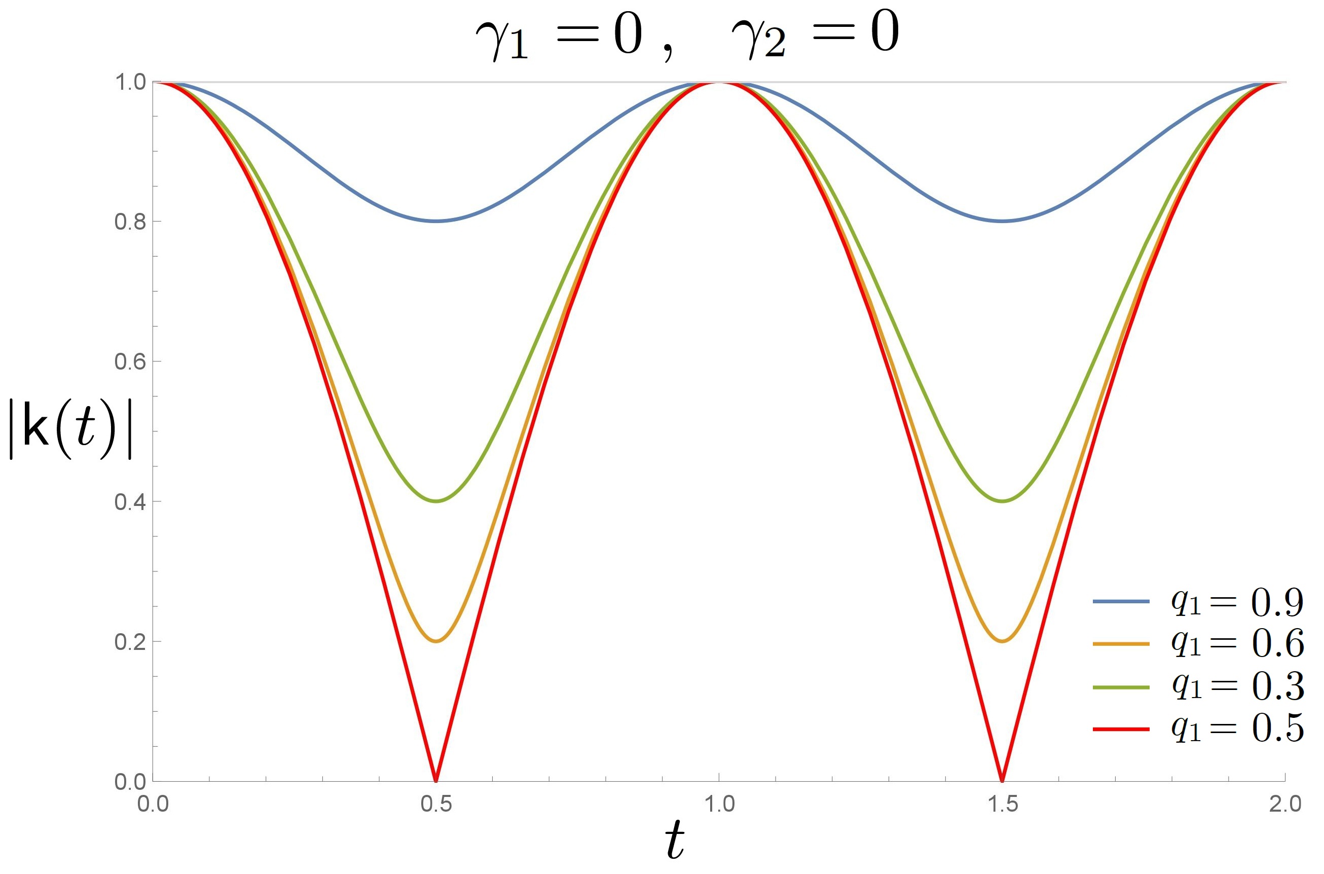
Figure 4: The distinguishability (LABEL:eq:osckappa) of optimal state pairs as a function of time for $\lambda_{1}=2\pi$ and $\lambda_{2}=0$, in the case $\gamma_{1}=\gamma_{2}=0$ corresponding to a random unitary map.

D.2 Information flow analysis

To further illustrate the dynamics let us consider equal weights $q_{1}=q_{2}=1/2$ in the convex mixture of dynamical processes, so that $\Phi_{t}$ is simply given by the average of $\Phi_{t}^{(1)}$ and $\Phi_{t}^{(2)}$. We choose $\gamma_{1}=\gamma_{2}=1/3$ and $\lambda_{1}=\pi/2$, $\lambda_{2}=0$ and, as initial states, the orthogonal pair of states

$$\rho_{S}^{1}=\frac{I_{S}+\sigma_{S}^{2}}{2},\qquad\rho_{S}^{2}=\frac{I_{S}-\sigma_{S}^{2}}{2},$$ (67)

which evolve in the equatorial plane of the Bloch sphere. In Figs. 5 and 6 we visualize the dynamics under the various maps and how the mixing process leads to non-Markovian dynamics.

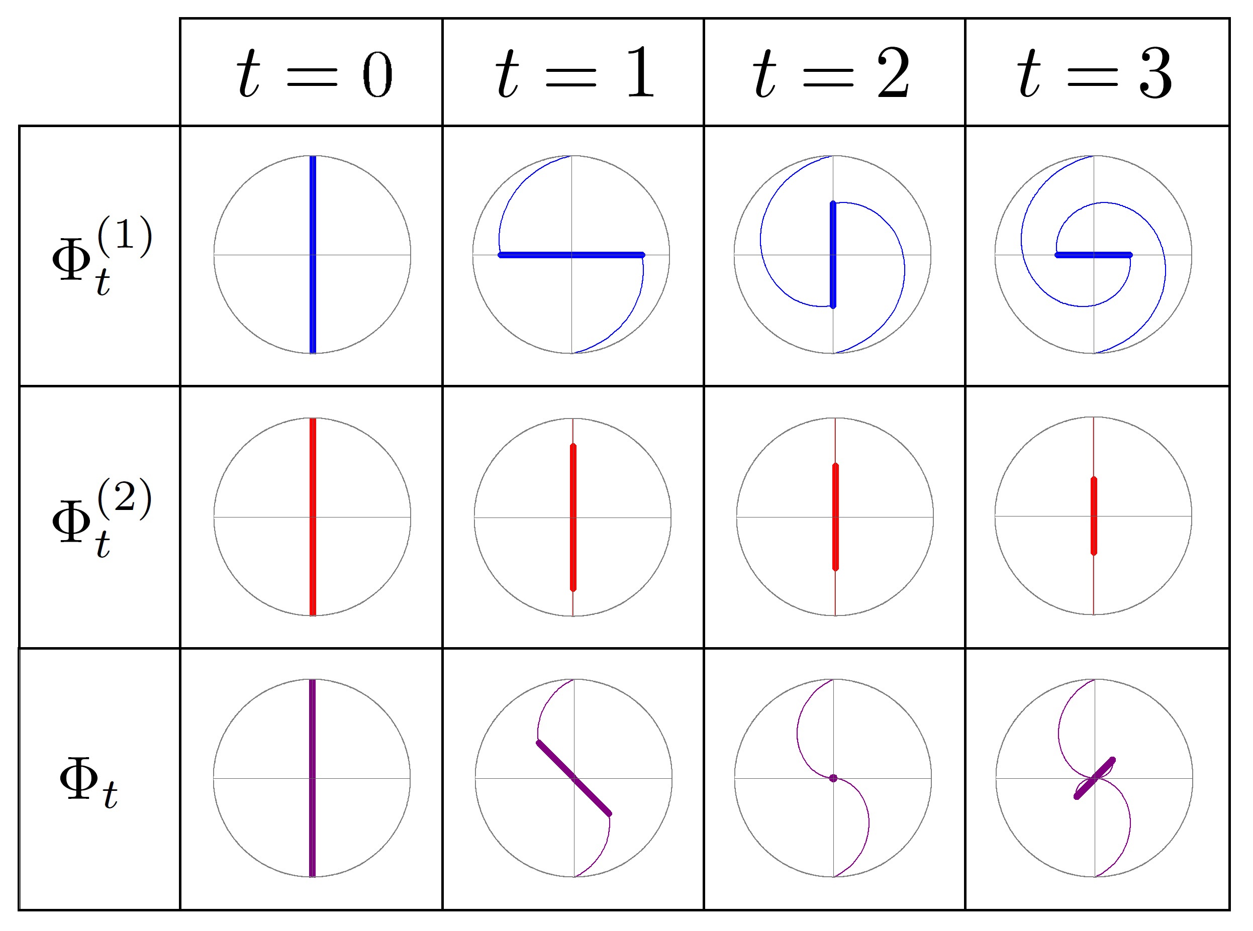
Figure 5: Dynamics of the initial states (67) under the maps $\Phi_{t}^{(1)}$, $\Phi_{t}^{(2)}$ and $\Phi_{t}$. The thin lines show the trajectories of the states, while the bold straight lines represent the trace distance at the given time. The semigroups $\Phi_{t}^{(1)}$ and $\Phi_{t}^{(2)}$ yield a monotonically decreasing distinguishability, while we obtain revivals of the distinguishability for the convex mixture $\Phi_{t}=\frac{1}{2}[\Phi_{t}^{(1)}+\Phi_{t}^{(2)}]$. In fact, the value of distinguishability decreases and reaches zero for $t=2$, as $\Phi_{t=2}[\rho_{S}^{1}]=\Phi_{t=2}[\rho_{S}^{2}]$, and then grows back to positive values at later times.

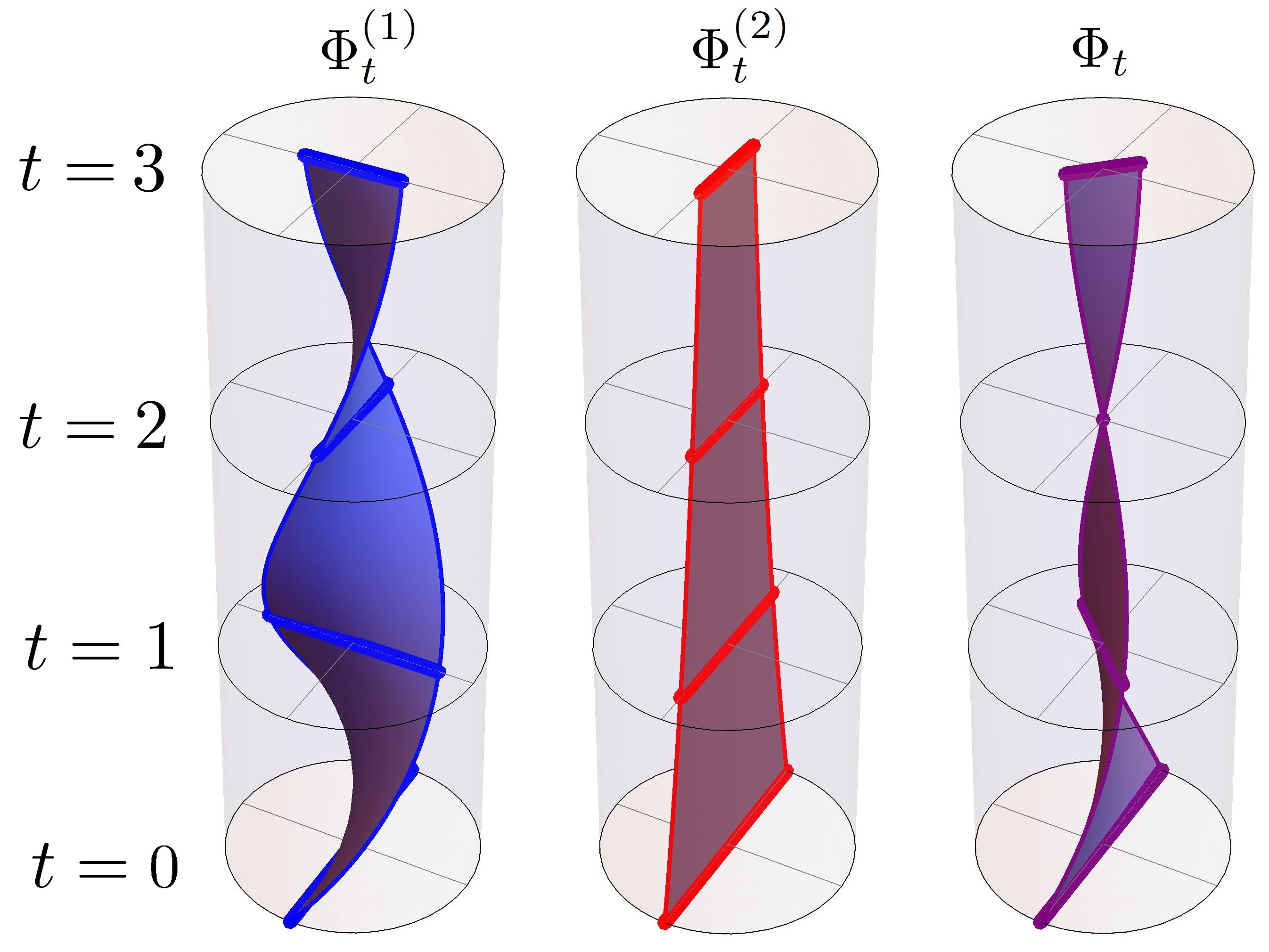
Figure 6: Visualization of the dynamics of the initial pair of states (67), together with their trace distance under the maps $\Phi_{t}^{(1)}$, $\Phi_{t}^{(2)}$ and $\Phi_{t}$. As in Fig. 5 we indicate the trace distance by straight bold lines at times $t=0,1,2,3$.

Let us analyze the flow of information by means of the quantities (see Eqs. (20) and (21) of the main text)

$$I_{\textrm{int}}(t) = \frac{1}{2}||\Phi_{t}[\rho_{S}^{1}-\rho_{S}^{2}]||,$$ (68)

$$I_{\textrm{tot}}(t) = I_{\textrm{int}}(t)+I_{\textrm{ext}}(t)=\frac{1}{2}||\Lambda_{t}[\rho_{S}^{1}-\rho_{S}^{2}]||.$$ (69)

For the choice (67) the internal information is given by $|\mathsf{k}(t)|$ which reads in this specific case

$$I_{\textrm{int}}(t)=e^{-t/3}|\cos(\pi t/4)|,$$ (70)

while using Eq. (15) of the main text we obtain

$$I_{\textrm{tot}}(t) = \frac{1}{2}||\Phi^{(1)}_{t}[\rho_{S}^{1}-\rho_{S}^{2}]||+\frac{1}{2}||\Phi^{(2)}_{t}[\rho_{S}^{1}-\rho_{S}^{2}]||$$ (71)

$$= \frac{1}{2}e^{-\gamma_{1}t}+\frac{1}{2}e^{-\gamma_{2}t}=e^{-t/3}.$$

These expressions are plotted in Fig. 7.

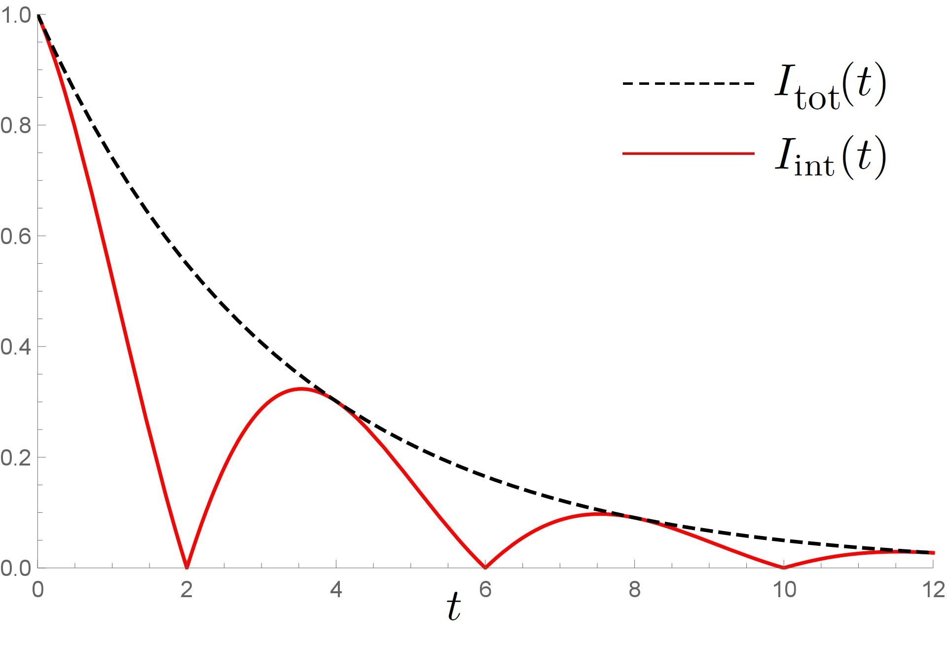
Figure 7: Internal and total information as functions of time. The internal information (70) oscillates and is bounded by the total information (71). Note the decrease of the total information, signalling the loss of information towards the dissipative environments generating the single semigroups $\Phi_{t}^{(1)}$ and $\Phi_{t}^{(2)}$.

Finally, we consider the external information

$$I_{\textrm{ext}}(t) = I_{\textrm{tot}}(t)-I_{\textrm{int}}(t)$$ (72)

$$= e^{-t/3}\left[1-|\cos(\pi t/4)|\right].$$

This quantity satisfies inequality (22) of the main text:

$$I_{\mathrm{ext}}(t)\leq D(\Lambda_{t}[\rho_{S}^{1}],\Phi_{t}[\rho_{S}^{1}]\otimes\rho_{A})+D(\Lambda_{t}[\rho_{S}^{2}],\Phi_{t}[\rho_{S}^{2}]\otimes\rho_{A}).$$ (73)

In the present case the right-hand side of this inequality is found to be (see Sec. D.3)

$$D(\Lambda_{t}[\rho_{S}^{1}],\Phi_{t}[\rho_{S}^{1}]\otimes\rho_{A})+D(\Lambda_{t}[\rho_{S}^{2}],\Phi_{t}[\rho_{S}^{2}]\otimes\rho_{A})$$

$$=e^{-t/3}|\sin(\pi t/4)|.$$ (74)

Inequality (73) is illustrated in Fig. 8.

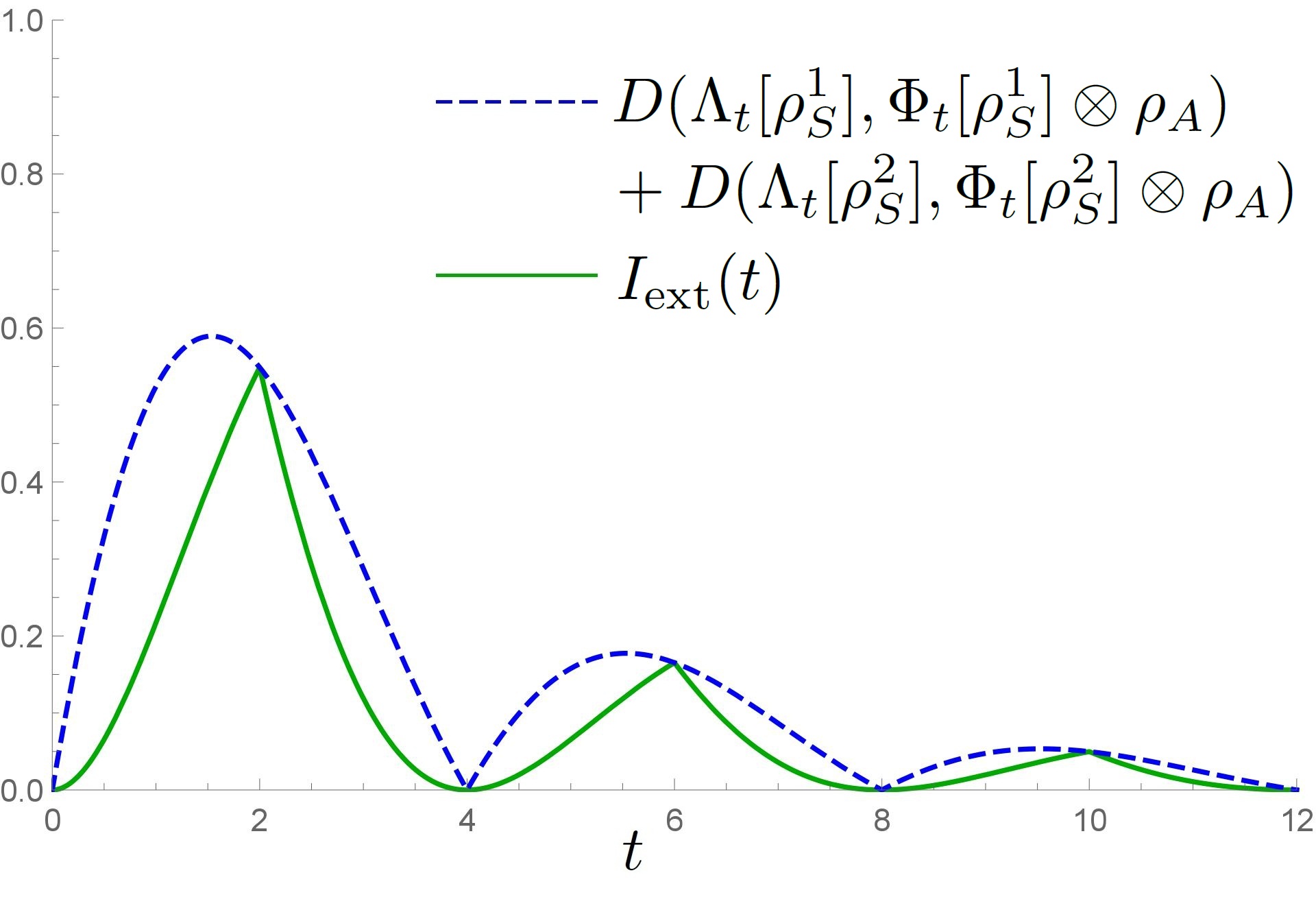
Figure 8: Illustration of inequality (73). Note that the bound for the external information (72) is tight, as the equality sign in (73) holds whenever $\cos(\pi t/2)=\pm 1$.

D.3 Proof of Eq. (74)

Lemma. Suppose we have a bipartite Hilbert space $\mathcal{H}_{S}\otimes\mathcal{H}_{A}$, a probability distribution $\{q_{i}\}$, a collection of statistical operators $\{\rho^{i}_{S}\}$ on $\mathcal{H}_{S}$, and a collection of orthogonal projections $\{\Pi_{i}\}$ on $\mathcal{H}_{A}$, where $i=1,2,\ldots,n$. Then, for composite states of the form

$$\rho_{SA}=\sum_{i}q_{i}\rho^{i}_{S}\otimes\Pi_{i}$$ (75)

the trace distance between the state and the product of its marginals obeys the bound

$$D(\rho_{SA},\rho_{S}\otimes\rho_{A})\leq 2\sum_{i>j}q_{i}q_{j}D(\rho^{i}_{S},\rho^{j}_{S}),$$ (76)

which is saturated for the case $n=2$

$$D(\rho_{SA},\rho_{S}\otimes\rho_{A})=2q_{1}q_{2}D(\rho^{1}_{S},\rho^{2}_{S}).$$ (77)

Proof. Orthogonality of the projections leads to the following identities

$$D(\rho_{SA},\rho_{S}\otimes\rho_{A}) = D(\sum_{i}q_{i}\rho^{i}_{S}\otimes\Pi_{i},\sum_{j}q_{j}\rho^{j}_{S}\otimes\sum_{i}q_{i}\Pi_{i})$$ (78)

$$= \frac{1}{2}\|\sum_{i}q_{i}\rho^{i}_{S}\otimes\Pi_{i}-\sum_{i,j}q_{j}q_{i}\rho^{j}_{S}\otimes\Pi_{i}\|$$

$$= \frac{1}{2}\|\sum_{i}q_{i}\{(1-q_{i})\rho^{i}_{S}-\sum_{j\neq i}q_{j}\rho^{j}_{S}\}\otimes\Pi_{i}\|$$

$$= \frac{1}{2}\sum_{i}q_{i}\|(1-q_{i})\rho^{i}_{S}-\sum_{j\neq i}q_{j}\rho^{j}_{S}\|$$

$$= \frac{1}{2}\sum_{i}q_{i}\|\sum_{j\neq i}q_{j}(\rho^{i}_{S}-\rho^{j}_{S})\|.$$

For $n=2$ a single term remains and we have the identity

$$D(\rho_{SA},\rho_{S}\otimes\rho_{A})=2q_{1}q_{2}D(\rho^{1}_{S},\rho^{2}_{S}),$$ (79)

for the general case the triangular inequality implies

$$D(\rho_{SA},\rho_{S}\otimes\rho_{A})\leq 2\sum_{i>j}q_{i}q_{j}D(\rho^{i}_{S},\rho^{j}_{S}),$$ (80)

which proves the lemma.

Using Eq. (79) for $q_{1}=q_{2}=1/2$ we find

$$D(\Lambda_{t}[\rho_{S}^{1}],\Phi_{t}[\rho_{S}^{1}]\otimes\rho_{A})+D(\Lambda_{t}[\rho_{S}^{2}],\Phi_{t}[\rho_{S}^{2}]\otimes\rho_{A})$$ (81)

$$=\frac{1}{2}D(\Phi^{(1)}_{t}[\rho_{S}^{1}],\Phi^{(2)}_{t}[\rho_{S}^{1}])+\frac{1}{2}D(\Phi^{(1)}_{t}[\rho_{S}^{2}],\Phi^{(2)}_{t}[\rho_{S}^{2}]).$$

Because of the symmetric time evolution of $\rho_{S}^{1}$ and $\rho_{S}^{2}$ under $\Phi^{(1)}_{t}$ and $\Phi^{(2)}_{t}$ (see Figs. 5 and 6) we have

$$D(\Phi^{(1)}_{t}[\rho_{S}^{1}],\Phi^{(2)}_{t}[\rho_{S}^{1}])=D(\Phi^{(1)}_{t}[\rho_{S}^{2}],\Phi^{(2)}_{t}[\rho_{S}^{2}])$$ (82)

and thus

$$D(\Lambda_{t}[\rho_{S}^{1}],\Phi_{t}[\rho_{S}^{1}]\otimes\rho_{A})+D(\Lambda_{t}[\rho_{S}^{2}],\Phi_{t}[\rho_{S}^{2}]\otimes\rho_{A})$$

$$=D(\Phi^{(1)}_{t}[\rho_{S}^{1}],\Phi^{(2)}_{t}[\rho_{S}^{1}]).$$ (83)

The trace distance $D(\Phi^{(1)}_{t}[\rho_{S}^{1}],\Phi^{(2)}_{t}[\rho_{S}^{1}])$ is easily found to be given by the expression

$$D(\Phi^{(1)}_{t}[\rho_{S}^{1}],\Phi^{(2)}_{t}[\rho_{S}^{1}])=e^{-t/3}|\sin(\pi t/4)|.$$ (84)

Substituting this into Eq. (83) we obtain Eq. (74).