ADI schemes for valuing European options under the Bates model

Abstract

This paper is concerned with the adaptation of alternating direction implicit (ADI) time discretization schemes for the numerical solution of partial integro-differential equations (PIDEs) with application to the Bates model in finance. Three different adaptations are formulated and their (von Neumann) stability is analyzed. Ample numerical experiments are provided for the Bates PIDE, illustrating the actual stability and convergence behaviour of the three adaptations.

Keywords:  partial integro-differential equations, operator splitting methods, alternating direction implicit schemes, stability, Bates model.

1 Introduction

The traditional asset price model in financial option valuation theory is the geometric Brownian motion. It is well-known that this model assumes constant volatility while the market prices of options clearly indicate varying volatility. For the valuation of options with long maturities, stochastic volatility models like the Heston stochastic volatility model [18] are a common means to introduce such variability. For short maturities, however, pure Brownian motion based models such as the Heston model often require excessively large volatilities to explain the market prices of options. A modern way to resolve this is to incorporate jumps in the asset price model, like the classical Merton jump-diffusion model [36] does. The Bates model [6] combines the Merton model and the Heston model. This asset price model includes both jumps and stochastic volatility and it is therefore popular for valuing options with short as well as long maturities.

Under the Bates model, a two-dimensional parabolic partial integro-differential equation (PIDE) can be derived for the values of European-style options with the spatial variables representing the underlying asset price and its instantaneous variance [9]. The differential operator is of the convection-diffusion type. The integral operator, which stems from the jumps, couples all option values in the asset price direction.

This paper deals with the numerical solution of the Bates PIDE. We follow the method of lines approach, where the PIDE is first discretized in the spatial variables and the resulting semidiscrete system of ordinary differential equations (ODEs) is solved by applying a suitable implicit time discretization scheme. Due to the nonlocal nature of the integral operator, semidiscretization leads to a large, dense system matrix. For an implicit time discretization scheme one thus faces two challenges: the efficient treatment of the two-dimensional convection-diffusion part and the efficient treatment of the dense integral part. In this paper we focus on operator splitting methods, which handle these two parts separately in an effective manner. The following reviews methods proposed in the literature.

For the time discretization of the two-dimensional partial differential equation (PDE) arising from the Heston model, various alternating direction implicit (ADI) schemes were studied in [23]. ADI and other directional splitting methods, see e.g. [21], are highly efficient. In each time step they yield a sequence of unidirectional linear systems, which can be solved very fast using LU factorization. Since the original papers [13, 14, 38], the literature on ADI schemes for time-dependent convection-diffusion equations is extensive. In financial option valuation, correlations between the underlying stochastic processes (asset price, variance) give rise to mixed spatial-derivative terms in the pertinent PDEs. First-order ADI schemes have been investigated for such PDEs in [34, 35] and second-order ADI schemes in [11, 17, 23, 24, 25, 26, 28, 29, 37], where the mixed derivative part is always treated in an explicit fashion.

Under the Merton model a one-dimensional PIDE for European option values holds. Application of a classical implicit time discretization scheme such as Crank–Nicolson or BDF2 leads in every time step to the solution of a linear system with a dense matrix. An iterative method requiring only multiplications by a dense matrix and solutions to tridiagonal systems can often solve these linear systems with a few iterations [1, 12, 39, 42]. Alternatively, a splitting method for the time discretization of the Merton PIDE was proposed in [2]. This method, of the Peaceman–Rachford type, treats the integral part in an implicit manner and employs FFT to reduce computational cost. An implicit-explicit (IMEX) method that treats the sparse diffusion part implicitly and the dense integral part explicitly was investigated in [10]. The pertinent method is only first-order. Second-order IMEX methods such as the IMEX midpoint and IMEX–CNAB (Crank–Nicolson Adams–Bashforth) schemes were subsequently investigated in [16, 33, 40] and IMEX schemes of the Runge–Kutta type were examined in [7].

The IMEX–CNAB method has been applied to the Bates PIDE in [41]. For the solution of the linear system in each time step, both LU factorization and an algebraic multigrid method were considered. An adaptive finite difference discretization combined with the IMEX–CNAB method and LU factorization was constructed in [44]. In [4, 5] a first-order directional splitting method was used together with Richardson extrapolation with the aim to obtain second-order accuracy. Directional splitting methods of the Strang type were studied in [8, 43]. In [31] the authors employed Strang splitting between the convection-diffusion and integrals parts and applied a second-order ADI scheme to solve the two-dimensional convection-diffusion substeps in this approach; see also [30]. A novel, direct adaptation of ADI schemes to two-dimensional PIDEs has recently been proposed in [32]. Here the integral and mixed derivative parts are treated jointly in an explicit fashion.

For more information on operator splitting methods like ADI and IMEX schemes in finance we refer to [22, 27]. A good general reference is [20].

In this paper we consider the adaptation of ADI schemes for the time discretization of two-dimensional PIDEs with the Bates model as the leading example. We formulate three types of adaptations: two of these are novel and one agrees with that from [32]. The obtained operator splitting methods are all of second-order and treat both the integral and mixed derivative parts in an explicit manner. At each time step they require only one or two multiplications with the dense matrix corresponding to the integral part. Hence, the resulting methods are computationally very efficient.

An outline of this paper is as follows. Section 2 describes the Bates model, the PIDE for European option values, and its spatial discretization. In Section 3 the three adaptations of ADI schemes to PIDEs are formulated and their stability is analyzed. Numerical experiments for these adaptations applied to the Bates PIDE are presented in Section 4. The conclusions end the paper in Section 5.

2 Bates model and its semidiscretization

We consider in this paper the Bates model [6], which merges the Heston stochastic volatility model [18] and the Merton jump-diffusion model [36] for the asset price $S_{\tau}\geq 0$. Here the instantaneous variance $V_{\tau}\geq 0$ follows a CIR process with mean-reversion level $\eta>0$, mean-reversion rate $\kappa>0$ and volatility-of-variance $\sigma>0$. The underlying Brownian motions for $S_{\tau}$ and $V_{\tau}$ have correlation $\rho\in[-1,1]$. The jump process is a compound Poisson process with intensity $\lambda>0$. The probability of a jump from $S_{\tau}$ to $S_{\tau}Y$ with random variable $Y>0$ is defined by the log-normal probability density function

$$f(y)=\frac{1}{y\delta\sqrt{2\pi}}e^{-\frac{(\log y-\gamma)^{2}}{2\delta^{2}}}\quad(y>0),$$

where $\gamma$ and $\delta$ are given real constants with $\delta>0$ that are equal to the mean and standard deviation, respectively, of the normal random variable $\log(Y)$. Let $r\geq 0$ be the risk-free interest rate and let $\varepsilon$ denote the mean relative jump size, given by $\varepsilon=e^{\gamma+\delta^{2}/2}-1$. Consider an European-style option with maturity time $T$. Under the Bates model, if $S_{T-t}=s$ and $V_{T-t}=v$, then the option value $u(s,v,t)$ satisfies the PIDE

$$\begin{split}\frac{\partial u}{\partial t}&{}=\frac{1}{2}s^{2}v\frac{\partial^{2}u}{\partial s^{2}}+\rho\sigma sv\frac{\partial^{2}u}{\partial s\partial v}+\frac{1}{2}\sigma^{2}v\frac{\partial^{2}u}{\partial v^{2}}+(r-\lambda\varepsilon)s\frac{\partial u}{\partial s}+\kappa(\eta-v)\frac{\partial u}{\partial v}\\ &{}-(r+\lambda)u+\lambda\int_{0}^{\infty}u(sy,v,t)f(y)dy\end{split}$$ (2.1)

whenever $s>0$, $v>0$, $0<t\leq T$. The initial condition for (2.1) is

$$u(s,v,0)=\phi(s),$$ (2.2)

where $\phi$ denotes the pay-off function, which specifies the value of the option at expiry. In this paper we shall consider vanilla put options. The pay-off function is then $\phi(s)=\max\{K-s,\,0\}$ with given strike price $K$.

For feasibility of the numerical solution, the unbounded spatial domain is truncated to $[0,\,S_{\max}]\times[0,\,V_{\max}]$ with sufficiently large $S_{\max}$ and $V_{\max}$ chosen such that the error caused by this truncation is negligible. We pose the Dirichlet and Neumann boundary conditions

$$\begin{split}u(0,v,t)&=e^{-rt}K\phantom{0}~{}~{}(0\leq v\leq V_{\max},\;0<t\leq T),\\ \phantom{\frac{\partial u}{\partial s}}u(S_{\max},v,t)&=0\phantom{e^{-rt}K}~{}~{}(0\leq v\leq V_{\max},\;0<t\leq T),\\ \frac{\partial u}{\partial v}(s,V_{\max},t)&=0\phantom{e^{-rt}K}~{}~{}(0\leq s\leq S_{\max},\;0<t\leq T),\end{split}$$ (2.3)

and at the boundary $v=0$ it is assumed that the PIDE (2.1) holds, compare [15].

For the spatial discretization on the computational domain $[0,\,S_{\max}]\times[0,\,V_{\max}]$ a smooth, nonuniform Cartesian grid is chosen with meshes in the $s$- and $v$-directions of the type considered in [17]. This grid has a large fraction of points in the neighbourhood of the important location $(s,v)=(K,0)$. Let the grid points in the $s$-direction be denoted by $0=s_{0}<s_{1}<\cdots<s_{m_{1}}=S_{\max}$ and the grid points in the $v$-direction by $0=v_{0}<v_{1}<\cdots<v_{m_{2}}=V_{\max}$. Let the mesh widths $\Delta s_{i}=s_{i}-s_{i-1}$, $\Delta v_{j}=v_{j}-v_{j-1}$ and write $u_{i,j}$ for the value of $u$ at grid point $(s_{i},v_{j})$. For the partial derivatives of $u$ with respect to $s$ we apply the standard central finite differences

$$\frac{\partial u_{i,j}}{\partial s}\approx\frac{-\Delta s_{i+1}}{\Delta s_{i}(\Delta s_{i}+\Delta s_{i+1})}\,u_{i-1,j}+\frac{\Delta s_{i+1}-\Delta s_{i}}{\Delta s_{i}\Delta s_{i+1}}\,u_{i,j}+\frac{\Delta s_{i}}{(\Delta s_{i}+\Delta s_{i+1})\Delta s_{i+1}}\,u_{i+1,j}$$ (2.4)

and

$$\frac{\partial^{2}u_{i,j}}{\partial s^{2}}\approx\frac{2}{\Delta s_{i}(\Delta s_{i}+\Delta s_{i+1})}\,u_{i-1,j}-\frac{2}{\Delta s_{i}\Delta s_{i+1}}\,u_{i,j}+\frac{2}{(\Delta s_{i}+\Delta s_{i+1})\Delta s_{i+1}}\,u_{i+1,j}\,.$$ (2.5)

For the partial derivatives of $u$ with respect to $v$ the analogous finite differences are considered, with the exception of the boundary $v=0$, where we apply the forward formula

$$\frac{\partial u_{i,0}}{\partial v}\approx-\frac{2{\Delta v}_{1}+{\Delta v}_{2}}{{\Delta v}_{1}({\Delta v}_{1}+{\Delta v}_{2})}\,u_{i,0}+\frac{{\Delta v}_{1}+{\Delta v}_{2}}{{\Delta v}_{1}{\Delta v}_{2}}\,u_{i,1}-\frac{{\Delta v}_{1}}{({\Delta v}_{1}+{\Delta v}_{2}){\Delta v}_{2}}\,u_{i,2}\,.$$ (2.6)

For the mixed derivative $\partial^{2}u/\partial s\partial v$ the central nine-point formula is used that is obtained by successive application of the standard central finite differences for the first derivative in the $s$- and $v$-directions.

For the discretization of the integral term in (2.1), we employ linear interpolation for $u$ between consecutive grid points in the $s$-direction, and $u(s,v,t)$ is approximated to be zero whenever $s\geq S_{\max}$. After some calculations, this leads to the quadrature rule

$$\begin{split}&\int_{0}^{\infty}u(s_{i}y,v_{j},\cdot)f(y)dy\\ &\approx\sum_{k=0}^{m_{1}-1}\frac{1}{2\Delta s_{k+1}}\left[\left(c_{1,i,k}s_{i}-c_{0,i,k}s_{k+1}\right)u_{k,j}+\left(c_{0,i,k}s_{k}-c_{1,i,k}s_{i}\right)u_{k+1,j}\right],\end{split}$$ (2.7)

where

$$c_{d,i,k}=e^{d(\gamma+\delta^{2}/2)}\left[\operatorname{erf}\left(\frac{\gamma+d\delta^{2}-\log(s_{k+1}/s_{i})}{\delta\sqrt{2}}\right)-\operatorname{erf}\left(\frac{\gamma+d\delta^{2}-\log(s_{k}/s_{i})}{\delta\sqrt{2}}\right)\right]$$ (2.8)

for $d=0,1$ with $\operatorname{erf}(\cdot)$ denoting the error function. This same approximation of the integral term was used in [39], for example. Here we adopt the convention $\log(0)=-\infty$ and $\operatorname{erf}(\infty)=1$.

Collecting the semidiscrete approximations to the grid point values $u(s_{i},v_{j},t)$ for $1\leq i\leq m_{1}-1$, $0\leq j\leq m_{2}$ into a vector $U(t)$ gives rise to a system of ODEs of the form

$$\dot{U}(t)={\boldsymbol{A}}U(t)+G(t),~{}~{}0<t\leq T.$$ (2.9)

Here ${\boldsymbol{A}}$ is a given $m\times m$-matrix and $G(t)$ is a given $m$-vector with $m=(m_{1}-1)(m_{2}+1)$. The vector $G(t)$ depends on the Dirichlet boundary data in (2.3). Let ${\boldsymbol{I}}$ denote the $m\times m$-identity matrix. The matrix ${\boldsymbol{A}}$ can be written as

$${\boldsymbol{A}}={\boldsymbol{D}}-(r+\lambda){\boldsymbol{I}}+\lambda{\boldsymbol{J}},$$ (2.10)

where ${\boldsymbol{D}}$ represents the convection-diffusion part of (2.1) and ${\boldsymbol{J}}$ represents the integral. The matrix ${\boldsymbol{D}}$ is sparse, whereas ${\boldsymbol{J}}$ is a block diagonal matrix with $m_{2}+1$ dense diagonal blocks of size $(m_{1}-1)\times(m_{1}-1)$. It can be shown that all entries of ${\boldsymbol{J}}$ are nonnegative and all its row sums are bounded from above by one. In particular this implies that the spectrum of ${\boldsymbol{J}}$ belongs to the complex unit disk.

The ODE system (2.9) is complemented with an initial vector $U(0)$ that is given by the values of the pay-off function $\phi$ at the spatial grid points where, in view of the nonsmoothness of $\phi$ at the strike $K$, the values at the grid points $(s_{i},v_{j})$ with $s_{i}$ the point lying closest to $K$ are replaced by the cell average value

$$\frac{1}{\Delta s_{i+1/2}}\int_{s_{i-1/2}}^{s_{i+1/2}}\phi(s)\,ds$$ (2.11)

with $s_{i-1/2}=\tfrac{1}{2}(s_{i-1}+s_{i}),s_{i+1/2}=\tfrac{1}{2}(s_{i}+s_{i+1}),\Delta s_{i+1/2}=s_{i+1/2}-s_{i-1/2}.$

3 Operator splitting methods

3.1 Adaptation of ADI schemes to PIDEs

For the efficient temporal discretization of the semidiscrete system (2.9) we study in this paper operator splitting methods. To this purpose, the matrix ${\boldsymbol{A}}$ is decomposed into four matrices,

$${\boldsymbol{A}}={\boldsymbol{A}}_{0}^{\rm(J)}+{\boldsymbol{A}}_{0}^{\rm(D)}+{\boldsymbol{A}}_{1}+{\boldsymbol{A}}_{2}.$$ (3.1)

Here ${\boldsymbol{A}}_{1}$, respectively ${\boldsymbol{A}}_{2}$, corresponds to the finite difference discretization of all spatial derivatives in the $s$-direction, respectively $v$-direction, minus half of the $(r+\lambda){\boldsymbol{I}}$ matrix. Next, ${\boldsymbol{A}}_{0}^{\rm(D)}$ represents the finite difference discretization of the mixed derivative term in (2.1) and ${\boldsymbol{A}}_{0}^{\rm(J)}=\lambda{\boldsymbol{J}}$ represents the finite difference discretization of the integral term. We note that incorporating $(r+\lambda){\boldsymbol{I}}$ in the above manner turns out to be beneficial for stability. The vector $G(t)$, containing the boundary contributions, is decomposed analogously to ${\boldsymbol{A}}$. It is convenient to define for $0\leq t\leq T$ and $V\in\mathbb{R}^{m}$,

$$\begin{split}{\bf F}_{0}^{\rm(J)}(t,V)&={\boldsymbol{A}}_{0}^{\rm(J)}V+G_{0}^{\rm(J)}(t),\\ \\ {\bf F}_{0}^{\rm(D)}(t,V)&={\boldsymbol{A}}_{0}^{\rm(D)}V+G_{0}^{\rm(D)}(t),\\ \\ {\bf F}_{1}(t,V)&={\boldsymbol{A}}_{1}V+G_{1}(t),\\ \\ {\bf F}_{2}(t,V)&={\boldsymbol{A}}_{2}V+G_{2}(t),\end{split}$$

and write ${\bf F}={\bf F}_{0}+{\bf F}_{1}+{\bf F}_{2}$, ${\bf F}_{0}={\bf F}_{0}^{\rm(J)}+{\bf F}_{0}^{\rm(D)}$ and ${\bf F}^{\rm(D)}={\bf F}_{0}^{\rm(D)}+{\bf F}_{1}+{\bf F}_{2}$.

The basis for the operator splitting approach under investigation in this paper is the class of ADI schemes, which is well-established in the literature for option valuation PDEs, without integral term. As a prominent representative of this class we select the Modified Craig–Sneyd (MCS) scheme, which was introduced in [29].

Let $\theta>0$ be a given parameter. Let step size $\Delta t=T/N$ with given integer $N\geq 1$ and temporal grid points $t_{n}=n\Delta t$ for $n=0,1,\ldots,N$. If the integral term is absent, then ${\bf F}_{0}={\bf F}_{0}^{\rm(D)}$ and the MCS scheme generates successively, in a one-step manner, approximations $U_{n}$ to $U(t_{n})$ for $n=1,2,\ldots,N$ by

$$\left\{\begin{array}[]{lll}Y_{0}=U_{n-1}+\Delta t\,{\bf F}(t_{n-1},U_{n-1}),\\ \\ Y_{j}=Y_{j-1}+\theta\Delta t\,({\bf F}_{j}(t_{n},Y_{j})-{\bf F}_{j}(t_{n-1},U_{n-1}))\quad(j=1,2),\\ \\ \widehat{Y}_{0}=Y_{0}+\theta\Delta t\,({\bf F}_{0}(t_{n},Y_{2})-{\bf F}_{0}(t_{n-1},U_{n-1})),\\ \\ \widetilde{Y}_{0}=\widehat{Y}_{0}+(\frac{1}{2}-\theta)\Delta t\,({\bf F}(t_{n},Y_{2})-{\bf F}(t_{n-1},U_{n-1})),\\ \\ \widetilde{Y}_{j}=\widetilde{Y}_{j-1}+\theta\Delta t\,({\bf F}_{j}(t_{n},\widetilde{Y}_{j})-{\bf F}_{j}(t_{n-1},U_{n-1}))\quad(j=1,2),\\ \\ U_{n}=\widetilde{Y}_{2}.\end{array}\right.$$ (3.2)

The MCS scheme has classical order of consistency (that is, for fixed nonstiff ODEs) equal to two for any parameter value $\theta$. The particular choice $\theta=\frac{1}{2}$ yields the Craig–Sneyd (CS) scheme, introduced in [11].

In the MCS scheme the ${\bf F}_{0}$ part is treated in an explicit fashion and the ${\bf F}_{1}$ and ${\bf F}_{2}$ parts are treated in an implicit fashion. In each step of the scheme four linear systems need to be solved, involving the two matrices ${\boldsymbol{I}}-\theta\Delta t{\boldsymbol{A}}_{j}$ for $j=1,2$. Since these two matrices are essentially tridiagonal (up to permutation), the linear systems can be solved very efficiently by using $LU$ factorizations, which can be computed upfront. Notice further that $\widehat{Y}_{0}$ and $\widetilde{Y}_{0}$ can be combined in (3.2), so that just two evaluations of ${\bf F}_{0}$ are required per time step.

We study three adaptations of the MCS scheme to PIDEs. The first adaptation  is straightforward. It consists of (3.2) with ${\bf F}_{0}={\bf F}_{0}^{\rm(J)}+{\bf F}_{0}^{\rm(D)}$ as defined above. The integral term is then conveniently treated in an explicit way, along with the mixed derivative term. This type of adaptation has recently been proposed in [32], where the (related) Hundsdorfer–Verwer ADI scheme, instead of the MCS scheme, was considered.

The second adaptation  of the MCS scheme to PIDEs is obtained by treating the integral term in a one-step, explicit, second-order fashion directly at the beginning of each time step:

$$\left\{\begin{array}[]{lll}X_{0}=U_{n-1}+\Delta t\,{\bf F}(t_{n-1},U_{n-1}),\\ \\ Y_{0}=X_{0}+\frac{1}{2}\Delta t\,({\bf F}_{0}^{\rm(J)}(t_{n},X_{0})-{\bf F}_{0}^{\rm(J)}(t_{n-1},U_{n-1})),\\ \\ Y_{j}=Y_{j-1}+\theta\Delta t\,({\bf F}_{j}(t_{n},Y_{j})-{\bf F}_{j}(t_{n-1},U_{n-1}))\quad(j=1,2),\\ \\ \widehat{Y}_{0}=Y_{0}+\theta\Delta t\,({\bf F}_{0}^{\rm(D)}(t_{n},Y_{2})-{\bf F}_{0}^{\rm(D)}(t_{n-1},U_{n-1})),\\ \\ \widetilde{Y}_{0}=\widehat{Y}_{0}+(\frac{1}{2}-\theta)\Delta t\,({\bf F}^{\rm(D)}(t_{n},Y_{2})-{\bf F}^{\rm(D)}(t_{n-1},U_{n-1})),\\ \\ \widetilde{Y}_{j}=\widetilde{Y}_{j-1}+\theta\Delta t\,({\bf F}_{j}(t_{n},\widetilde{Y}_{j})-{\bf F}_{j}(t_{n-1},U_{n-1}))\quad(j=1,2),\\ \\ U_{n}=\widetilde{Y}_{2}.\end{array}\right.$$ (3.3)

We mention that the scheme defined by the first three lines of (3.3) followed by $U_{n}=Y_{2}$ has recently been studied, in a different context, in [3] for problems without integral term.

In the third adaptation  of the MCS scheme to PIDEs, the integral term is treated in a two-step, explicit, second-order fashion directly at the start of each time step:

$$\left\{\begin{array}[]{lll}X_{0}=U_{n-1}+\Delta t\,{\bf F}^{\rm(D)}(t_{n-1},U_{n-1}),\\ \\ Y_{0}=X_{0}+\frac{3}{2}\Delta t\,{\bf F}_{0}^{\rm(J)}(t_{n-1},U_{n-1})-\frac{1}{2}\Delta t\,{\bf F}_{0}^{\rm(J)}(t_{n-2},U_{n-2}),\\ \\ Y_{j}=Y_{j-1}+\theta\Delta t\,({\bf F}_{j}(t_{n},Y_{j})-{\bf F}_{j}(t_{n-1},U_{n-1}))\quad(j=1,2),\\ \\ \widehat{Y}_{0}=Y_{0}+\theta\Delta t\,({\bf F}_{0}^{\rm(D)}(t_{n},Y_{2})-{\bf F}_{0}^{\rm(D)}(t_{n-1},U_{n-1})),\\ \\ \widetilde{Y}_{0}=\widehat{Y}_{0}+(\frac{1}{2}-\theta)\Delta t\,({\bf F}^{\rm(D)}(t_{n},Y_{2})-{\bf F}^{\rm(D)}(t_{n-1},U_{n-1})),\\ \\ \widetilde{Y}_{j}=\widetilde{Y}_{j-1}+\theta\Delta t\,({\bf F}_{j}(t_{n},\widetilde{Y}_{j})-{\bf F}_{j}(t_{n-1},U_{n-1}))\quad(j=1,2),\\ \\ U_{n}=\widetilde{Y}_{2}.\end{array}\right.$$ (3.4)

For starting (3.4), we define $U_{1}$ by (3.2).

It can be shown that each of the adaptations (3.2), (3.3), (3.4) of the MCS scheme retains classical order of consistency equal to two for any value $\theta$. The mixed derivative and integral terms are always handled in an explicit manner. In (3.2) and (3.3) the integral term is dealt with in an explicit trapezoidal rule fashion, whereas in (3.4) it is treated in a two-step Adams–Bashforth fashion. An advantage of the adaptation (3.4) is that only one multiplication with the dense matrix ${\boldsymbol{A}}_{0}^{\rm(J)}$ is required per time step, instead of two for (3.2) and (3.3). Treating the integral term in a two-step Adams–Bashforth fashion has recently been advocated in [40, 41] where IMEX multistep schemes, without directional splitting, were considered for option valuation PIDEs.

In the following section we analyze the stability of the three adaptations of the MCS scheme.

3.2 Stability analysis

Let $\lambda_{0}$, $\mu_{0}$, $\mu_{1}$, $\mu_{2}$ denote any given complex numbers representing eigenvalues of the matrices ${\boldsymbol{A}}_{0}^{\rm(J)}$, ${\boldsymbol{A}}_{0}^{\rm(D)}$, ${\boldsymbol{A}}_{1}$, ${\boldsymbol{A}}_{2}$, respectively. For the stability analysis of the adaptations of the MCS scheme to PIDEs formulated in Section 3.1 we consider the linear scalar test equation

$$\dot{U}(t)=(\lambda_{0}+\mu_{0}+\mu_{1}+\mu_{2})\,U(t).$$ (3.5)

Let $w_{0}=\lambda_{0}\,\Delta t$ and $z_{j}=\mu_{j}\,\Delta t$ for $j=0,1,2$. Application of the three adaptations (3.2), (3.3), (3.4) to test equation (3.5) yields the linear recurrence relations

$$U_{n}=R(w_{0},z_{0},z_{1},z_{2})\,U_{n-1}\,,$$ (3.6)

$$U_{n}=S(w_{0},z_{0},z_{1},z_{2})\,U_{n-1}\,,$$ (3.7)

and

$$U_{n}=T_{1}(w_{0},z_{0},z_{1},z_{2})\,U_{n-1}+T_{0}(w_{0},z_{0},z_{1},z_{2})\,U_{n-2}\,,$$ (3.8)

respectively, with

$$R(w_{0},z_{0},z_{1},z_{2}) = 1+\frac{z}{p}+\theta\frac{(w_{0}+z_{0})z}{p^{2}}+(\tfrac{1}{2}-\theta)\frac{z^{2}}{p^{2}}\,,$$ (3.9)

$$S(w_{0},z_{0},z_{1},z_{2}) = 1+(1+\tfrac{1}{2}w_{0})\left(\frac{z}{p}+\theta\frac{z_{0}z}{p^{2}}+(\tfrac{1}{2}-\theta)\frac{(z_{0}+z_{1}+z_{2})z}{p^{2}}\right),~{}~{}~{}~{}~{}$$ (3.10)

$$T_{1}(w_{0},z_{0},z_{1},z_{2}) = 1+(z+\tfrac{1}{2}w_{0})\left(\frac{1}{p}+\theta\frac{z_{0}}{p^{2}}+(\tfrac{1}{2}-\theta)\frac{z_{0}+z_{1}+z_{2}}{p^{2}}\right),$$ (3.11)

$$T_{0}(w_{0},z_{0},z_{1},z_{2}) = -\tfrac{1}{2}w_{0}\left(\frac{1}{p}+\theta\frac{z_{0}}{p^{2}}+(\tfrac{1}{2}-\theta)\frac{z_{0}+z_{1}+z_{2}}{p^{2}}\right),$$ (3.12)

where

$$z=w_{0}+z_{0}+z_{1}+z_{2}\quad\text{and}\quad p=(1-\theta z_{1})(1-\theta z_{2}).$$

Clearly, if $w_{0}=0$, then $R$, $S$, $T_{1}$ reduce to the same rational function and $T_{0}$ vanishes.

We investigate the stability of the three processes (3.6), (3.7), (3.8). By definition of ${\boldsymbol{A}}_{j}$ it holds for $j=1,2$ that

$$\mu_{j}={\widetilde{\mu}}_{j}-\tfrac{1}{2}(r+\lambda),$$

where ${\widetilde{\mu}}_{j}$ represents an eigenvalue of the matrix corresponding to the finite difference discretization of all spatial derivatives in the $j$-th spatial direction. Let ${\widetilde{z}}_{j}={\widetilde{\mu}}_{j}\,\Delta t$ for $j=1,2$. In the stability analysis of ADI schemes for two-dimensional convection-diffusion equations with mixed derivative term, the following condition on $z_{0}$, ${\widetilde{z}}_{1}$, ${\widetilde{z}}_{2}$ plays a key role:

$$|z_{0}|\leq 2\sqrt{\Re{\widetilde{z}}_{1}\Re{\widetilde{z}}_{2}}~{}~{}{\rm and}~{}~{}\Re{\widetilde{z}}_{1}\leq 0,~{}\Re{\widetilde{z}}_{2}\leq 0,$$ (3.13)

where $\Re$ designates the real part. It is satisfied [28] in the model (von Neumann) framework, with semidiscretization by second-order central finite differences on uniform, Cartesian grids and periodic boundary condition. Consider the following, related condition on $w_{0}$, $z_{0}$, $z_{1}$, $z_{2}$ :

$$|z_{0}|+|w_{0}|\leq 2\sqrt{\Re z_{1}\Re z_{2}}~{}~{}{\rm and}~{}~{}\Re z_{1}\leq-\tfrac{1}{2}|w_{0}|,~{}\Re z_{2}\leq-\tfrac{1}{2}|w_{0}|.$$ (3.14)

For the integral term there holds

$$\lambda_{0}=\lambda\nu,$$

where $\nu\in\mathbb{C}$ represents an eigenvalue of the matrix ${\boldsymbol{J}}$. A natural assumption on $\nu$ is

$$|\nu|\leq 1,$$

compare Section 2. For $w_{0}$, $z_{0}$, $z_{1}$, $z_{2}$, ${\widetilde{z}}_{1}$, ${\widetilde{z}}_{2}$ defined above, we have the following useful lemma.

Lemma 3.1.

If $|\nu|\leq 1$, then  $\eqref{cond1}\Longrightarrow\eqref{cond2}$.

Proof.

Assume (3.13). Set $x=\lambda\Delta t$ and $y=(r+\lambda)\Delta t$, then $0\leq x\leq y$ and

$$w_{0}=x\nu,~{}~{}z_{1}={\widetilde{z}}_{1}-\tfrac{1}{2}y,~{}~{}z_{2}={\widetilde{z}}_{2}-\tfrac{1}{2}y.$$

It is obvious that $\Re z_{1}\leq-\tfrac{1}{2}|w_{0}|$ and $\Re z_{2}\leq-\tfrac{1}{2}|w_{0}|$. Next,

$$(|z_{0}|+|w_{0}|)^{2}\leq(|z_{0}|+x)^{2}\leq(|z_{0}|+y)^{2}\leq 4\Re{\widetilde{z}}_{1}\Re{\widetilde{z}}_{2}+4y\sqrt{\Re{\widetilde{z}}_{1}\Re{\widetilde{z}}_{2}}+y^{2}.$$

Using that

$$2\sqrt{\Re{\widetilde{z}}_{1}\Re{\widetilde{z}}_{2}}\leq-(\Re{\widetilde{z}}_{1}+\Re{\widetilde{z}}_{2})$$

there follows

$$(|z_{0}|+|w_{0}|)^{2}\leq 4\Re{\widetilde{z}}_{1}\Re{\widetilde{z}}_{2}-2y(\Re{\widetilde{z}}_{1}+\Re{\widetilde{z}}_{2})+y^{2}=4\Re z_{1}\Re z_{2}$$

and thus (3.14) is fulfilled. ∎

Write ${\widetilde{z}}_{0}=z_{0}+w_{0}$. For the adaptation (3.2) it clearly holds that

$$R(w_{0},z_{0},z_{1},z_{2})=R(0,{\widetilde{z}}_{0},z_{1},z_{2}).$$

In the literature on the stability analysis of the MCS scheme pertinent to PDEs with mixed derivative terms, a variety of favourable results has been derived on the stability bound $|R(0,{\widetilde{z}}_{0},z_{1},z_{2})|\leq 1$ under the condition

$$|{\widetilde{z}}_{0}|\leq 2\sqrt{\Re z_{1}\Re z_{2}}~{}~{}{\rm and}~{}~{}\Re z_{1}\leq 0,~{}\Re z_{2}\leq 0.$$ (3.15)

Obviously, (3.15) is weaker than (3.14). Hence, by virtue of Lemma 3.1, one directly arrives at positive stability results for the adaptation (3.2) pertinent to two-dimensional PIDEs with mixed derivative term. The following theorem gives two main results, which are relevant to diffusion-dominated and convection-dominated problems, respectively.

Theorem 3.2.

For the adaptation (3.2) there holds:

• If $\theta\geq\frac{1}{3}$, then $|R(w_{0},z_{0},z_{1},z_{2})|\leq 1$ whenever $w_{0},z_{0},z_{1},z_{2}\in\mathbb{R}$ satisfy (3.14).

• If $\frac{1}{2}\leq\theta\leq 1$, then $|R(w_{0},z_{0},z_{1},z_{2})|\leq 1$ whenever $w_{0},z_{0},z_{1},z_{2}\in\mathbb{C}$ satisfy (3.14).

The above theorem guarantees unconditional contractivity (that is, without any restriction on the spatial mesh width or temporal step size) for all jump intensities $\lambda$. It covers the most common values $\theta$ for the MCS scheme employed in the literature, namely $\theta=\frac{1}{3}$ and $\theta=\frac{1}{2}$. Parts (a) and (b) of Theorem 3.2 stem from [29, Thm. 2.5] and [25, Thm. 2.7], respectively. For various extensions and refinements of these stability results, we refer to [25, 26, 29, 37].

The interesting question arises whether similar positive results as Theorem 3.2 are valid for the adaptations (3.3) and (3.4). The first result is negative:

Theorem 3.3.

For the adaptation (3.3) there holds:

• If $|S(w_{0},z_{0},z_{1},z_{2})|\leq 1$ whenever $w_{0},z_{0},z_{1},z_{2}\in\mathbb{R}$ satisfy (3.14) and $w_{0}\geq 0$, then $\theta\geq\frac{1}{2}\sqrt{2}$.

• There exists no $\theta$ such that $|S(w_{0},z_{0},z_{1},z_{2})|\leq 1$ for all $w_{0},z_{0},z_{1},z_{2}\in\mathbb{R}$ satisfying (3.14).

Proof.

(a) Let $w_{0}=x\geq 0$ and consider $z_{0}=0$, $z_{1}=-\frac{1}{2}x-\xi$, $z_{2}=-\frac{1}{2}x$ with $\xi\geq 0$. Then (3.14) is fulfilled and

$$S(w_{0},z_{0},z_{1},z_{2})=1-\frac{(1+\tfrac{1}{2}x)\xi}{(1+\tfrac{\theta}{2}x+\theta\xi)(1+\tfrac{\theta}{2}x)}\left[1-\frac{(\tfrac{1}{2}-\theta)(x+\xi)}{(1+\tfrac{\theta}{2}x+\theta\xi)(1+\tfrac{\theta}{2}x)}\right].$$

Letting successively $\xi\rightarrow\infty$ and $x\rightarrow\infty$, the right-hand side tends to the value $1-1/\theta^{2}$. The modulus of this must be bounded from above by $1$, which yields $\theta\geq\frac{1}{2}\sqrt{2}$.

(b) Taking $w_{0}=-x\leq 0$, an analogous derivation as in (a) leads to the requirement that $1+1/\theta^{2}$ must be bounded from above by $1$, which obviously does not hold. ∎

Clearly, in Theorem 3.3 for the adaptation (3.3) the popular values $\theta=\frac{1}{3}$ and $\theta=\frac{1}{2}$ are excluded. We remark that the condition $w_{0}\in\mathbb{R}$, $w_{0}\geq 0$ is relevant to the case where the eigenvalues $\nu$ of ${\boldsymbol{J}}$ are real and lie in the interval $[0,1]$. This is often seen to be numerically fulfilled in our applications, compare Section 4.

For the adaptation (3.4), stability is determined by power-boundedness of the companion matrix

$$C(w_{0},z_{0},z_{1},z_{2})=\begin{pmatrix}\,T_{1}(w_{0},z_{0},z_{1},z_{2})&T_{0}(w_{0},z_{0},z_{1},z_{2})\,\\ 1&0\end{pmatrix}.$$

This is established by studying the roots of the characteristic polynomial

$$P(\zeta;w_{0},z_{0},z_{1},z_{2})=\zeta^{2}-T_{1}(w_{0},z_{0},z_{1},z_{2})\zeta-T_{0}(w_{0},z_{0},z_{1},z_{2}).$$

For any given point $(w_{0},z_{0},z_{1},z_{2})$ the recurrence relation (3.8) is stable if and only if the root condition holds: both roots $\zeta$ of $P$ have a modulus of at most one, and those with modulus equal to one are simple. If $T_{0}=T_{0}(w_{0},z_{0},z_{1},z_{2})$ and $T_{1}=T_{1}(w_{0},z_{0},z_{1},z_{2})$ are real, then by the Schur criterion the root condition is satisfied if and only if

$$|T_{0}|\leq 1~{}~{}{\rm and}~{}~{}T_{0}+|T_{1}|\leq 1$$ (3.16)

and there is no multiple root with modulus equal to one.

Theorem 3.4.

For the adaptation (3.4) there holds:

• If $\theta\geq\frac{1}{3}$, then (3.8) is stable whenever $w_{0},z_{0},z_{1},z_{2}\in\mathbb{R}$ satisfy (3.14) and $w_{0}\geq 0$.

• If (3.8) is stable whenever $w_{0},z_{0},z_{1},z_{2}\in\mathbb{R}$ satisfy (3.14), then $\theta\geq(9+\sqrt{33})/16$.

Proof.

(a) Write $R_{0}=R(0,z_{0},z_{1},z_{2})$. Condition (3.14) implies

$$|z_{0}|\leq 2\sqrt{z_{1}z_{2}}~{}~{}{\rm and}~{}~{}z_{1}\leq 0,~{}z_{2}\leq 0$$

and by [29, Thm. 2.5] it holds that $-1\leq R_{0}\leq 1$.

If $w_{0}=0$, then $T_{0}=0$ and $T_{1}=R_{0}$ and the root condition is clearly fulfilled. Assume next $w_{0}>0$. Using (3.14) yields

$$z=w_{0}+z_{0}+z_{1}+z_{2}\leq 2\sqrt{z_{1}z_{2}}+z_{1}+z_{2}=-\left(\sqrt{-z_{1}}-\sqrt{-z_{2}}\right)^{2}\leq 0$$

and thus

$$0<w_{0}\leq-(z_{0}+z_{1}+z_{2})=|z_{0}+z_{1}+z_{2}|.$$

We have

$$T_{0}=-\frac{\tfrac{1}{2}w_{0}}{z_{0}+z_{1}+z_{2}}(R_{0}-1)~{}~{}{\rm and}~{}~{}T_{1}=1+\frac{z+\tfrac{1}{2}w_{0}}{z_{0}+z_{1}+z_{2}}(R_{0}-1).$$ (3.17)

Hence,

$$|T_{0}|\leq\tfrac{1}{2}\left|R_{0}-1\right|\leq 1,$$

which proves the first condition in (3.16). Next,

$$T_{0}+T_{1}=1+\frac{z}{z_{0}+z_{1}+z_{2}}(R_{0}-1)\leq 1,$$

since $z_{0}+z_{1}+z_{2}<0$, $z\leq 0$ and $R_{0}\leq 1$. Subsequently,

$$T_{0}-T_{1}=-1-\frac{z+w_{0}}{z_{0}+z_{1}+z_{2}}(R_{0}-1)=-R_{0}-\frac{2w_{0}}{z_{0}+z_{1}+z_{2}}(R_{0}-1)\leq 1,$$

since $w_{0}>0$, $z_{0}+z_{1}+z_{2}<0$ and $-1\leq R_{0}\leq 1$. This proves the second condition in (3.16).

Finally, suppose $\zeta_{0}$ is a double root of $P$ with modulus one. Since the coefficients of $P$ are real, it must hold that $\zeta_{0}\in\{-1,1\}$ and consequently $T_{0}=-1$ and $T_{1}\in\{-2,2\}$. Using the expressions (3.17), the case $(T_{0},T_{1})=(-1,-2)$ leads to $R_{0}=-5$, which is a contradiction. Next, the case $(T_{0},T_{1})=(-1,2)$ implies $z=0$ and $R_{0}=-1$, which is also a contradiction, cf. (3.9). Thus there is no multiple root with modulus one.

(b) Let $w_{0}=-2/\theta$, $z_{0}=0$, $z_{1}=z_{2}=-1/\theta$. Then (3.14) is fulfilled and the necessary condition

$$T_{0}-T_{1}=-R_{0}-\frac{2w_{0}}{z_{0}+z_{1}+z_{2}}(R_{0}-1)=-R_{0}-2(R_{0}-1)\leq 1$$

becomes $R_{0}\geq\tfrac{1}{3}$. There holds

$$R_{0}=1-\frac{1}{2\theta}+\left(\frac{1}{2}-\theta\right)\frac{1}{4\theta^{2}}\,.$$

A simple calculation leads to the requirement that $8\theta^{2}-9\theta+\tfrac{3}{2}\geq 0$, which is readily seen to imply $\theta\geq(9+\sqrt{33})/16$. ∎

Part (a) of Theorem 3.4 for the adaptation (3.4) is a positive result and includes the common values $\theta=\frac{1}{3}\,,\,\frac{1}{2}$. Part (b) of the theorem is not favourable, on the other hand, given the (large) lower bound $(9+\sqrt{33})/16\approx 0.92$.

In the following we derive positive conclusions on the stability of both adaptations (3.3), (3.4) under the assumption that $\lambda T$ is of moderate size. These are obtained by a perturbation-type argument with respect to $w_{0}$, as employed in [32]. Define

$$Q(z_{0},z_{1},z_{2})=\frac{1}{p}+\theta\frac{z_{0}}{p^{2}}+(\tfrac{1}{2}-\theta)\frac{z_{0}+z_{1}+z_{2}}{p^{2}}\,,$$ (3.18)

and consider the condition

$$|z_{0}|\leq 2\sqrt{\Re z_{1}\Re z_{2}}~{}~{}{\rm and}~{}~{}\Re z_{1}\leq 0,~{}\Re z_{2}\leq 0,$$ (3.19)

which is clearly valid under (3.13).

Lemma 3.5.

Let $L=\max\{1/\theta\,,\,2\}$. Then $|Q(z_{0},z_{1},z_{2})|\leq L$ whenever (3.19) holds.

Proof.

It is easily seen that $|p|\geq 1$ and $|z_{0}|\leq|z_{1}+z_{2}|$. Hence,

$$|Q(z_{0},z_{1},z_{2})|\leq\left|1+\frac{z_{0}}{2p}+\left(\tfrac{1}{2}-\theta\right)\frac{z_{1}+z_{2}}{p}\right|\leq 1+\left(\tfrac{1}{2}+\left|\tfrac{1}{2}-\theta\right|\right)\left|\frac{z_{1}+z_{2}}{p}\right|.$$

Next, it can be verified that $|p|\geq\theta|z_{1}+z_{2}|$ and therefore

$$|Q(z_{0},z_{1},z_{2})|\leq 1+\left(\tfrac{1}{2}+\left|\tfrac{1}{2}-\theta\right|\right)\!/\theta=\max\{1/\theta\,,\,2\}.$$

∎

Theorem 3.6.

Let $M=e^{(1+L)\lambda T}$ and $n\Delta t\leq T$. For the adaptation (3.3) there holds:

• If $\theta\geq\frac{1}{3}$, then $|S(w_{0},z_{0},z_{1},z_{2})^{n}|\leq M$ whenever $|w_{0}|\leq\lambda\Delta t$ and $z_{0},z_{1},z_{2}\in\mathbb{R}$ satisfy (3.19).

• If $\frac{1}{2}\leq\theta\leq 1$, then $|S(w_{0},z_{0},z_{1},z_{2})^{n}|\leq M$ whenever $|w_{0}|\leq\lambda\Delta t$ and $z_{0},z_{1},z_{2}\in\mathbb{C}$ satisfy (3.19).

Proof.

Write $R_{0}=R(0,z_{0},z_{1},z_{2})$ as before. Upon inserting $z=w_{0}+(z_{0}+z_{1}+z_{2})$ into (3.10), it is readily shown that $S=S(w_{0},z_{0},z_{1},z_{2})$ can be expressed as

$$S=R_{0}+\left[\tfrac{1}{2}(R_{0}-1)+Q\right]\!w_{0}+\tfrac{1}{2}Qw_{0}^{2}.$$

Assume $|R_{0}|\leq 1$. Then, by applying Lemma 3.5,

$$|S|\leq 1+(1+L)|w_{0}|+\tfrac{1}{2}L|w_{0}|^{2}\leq e^{(1+L)|w_{0}|}\leq e^{(1+L)|w_{0}|}\leq e^{(1+L)\lambda\Delta t}.$$

Consequently, for $n\Delta t\leq T$,

$$|S^{n}|\leq e^{(1+L)\lambda T}=M.$$

Parts (a) and (b) now follow by virtue of [29, Thm. 2.5] and [25, Thm. 2.7], respectively. ∎

Denote by $\|\cdot\|$ the maximum norm for matrices.

Theorem 3.7.

Let $M=e^{2L\lambda T}$ and $n\Delta t\leq T$. For the adaptation (3.4) there holds:

• If $\theta\geq\frac{1}{3}$, then $\|C(w_{0},z_{0},z_{1},z_{2})^{n}\|\leq M$ whenever $|w_{0}|\leq\lambda\Delta t$ and $z_{0},z_{1},z_{2}\in\mathbb{R}$ satisfy (3.19).

• If $\frac{1}{2}\leq\theta\leq 1$, then $\|C(w_{0},z_{0},z_{1},z_{2})^{n}\|\leq M$ whenever $|w_{0}|\leq\lambda\Delta t$ and $z_{0},z_{1},z_{2}\in\mathbb{C}$ satisfy (3.19).

Proof.

From (3.11), (3.12) it is directly clear that

$$C=C(w_{0},z_{0},z_{1},z_{2})=\begin{pmatrix}R_{0}&0\,\\ 1&0\end{pmatrix}+\begin{pmatrix}\tfrac{3}{2}Qw_{0}&-\tfrac{1}{2}Qw_{0}\\ 0&0\end{pmatrix}.$$

Assume $|R_{0}|\leq 1$. Then, by Lemma 3.5,

$$\|C\|\leq 1+2L|w_{0}|\leq e^{2L|w_{0}|}\leq e^{2L\lambda\Delta t}$$

and the remainder of the proof is the same as that of Theorem 3.6. ∎

4 Numerical examples

In this section we examine by numerical experiments the stability and convergence behaviour of the three adaptations (3.2), (3.3), (3.4) of the MCS scheme in the application to the semidiscretized Bates PIDE described in Section 2. We consider the four parameter sets for the Bates model and European put option listed in Table 1. Case I has been considered in e.g. [41, 44] and Case II in [4, 5]. Case III stems from the recent monograph [30]. Case IV is new and has been constructed as a specifically challenging example, where in particular $\lambda T$ is large and the Feller condition $2\kappa\eta>\sigma^{2}$ is violated.

	Case I	Case II	Case III	Case IV
$\kappa$	2	2	1.5	2.5
$\eta$	0.04	0.04	0.1	0.05
$\sigma$	0.25	0.4	0.3	0.6
$\rho$	-0.5	-0.5	-0.5	-0.8
$r$	0.03	0.03	0.05	0.01
$\lambda$	0.2	5	5	10
$\gamma$	-0.5	-0.005	0.3	-0.05
$\delta$	0.4	0.1	0.1	0.01
$T$	0.5	0.5	1	5
$K$	100	100	100	100

Table 1: Parameter sets for the Bates model and European put option.

For the MCS scheme the common parameter values $\theta=\frac{1}{3}$ and $\theta=\frac{1}{2}$ are selected. Recall that the latter choice yields the Craig–Sneyd (CS) scheme. In addition, we study the reduced version of each of (3.2), (3.3), (3.4) that ends directly with the computation of $Y_{2}$ and sets $U_{n}=Y_{2}$. These can be viewed as adaptations of the well-known Douglas (Do) scheme (cf. e.g. [19, 20, 28]) and will be applied with $\theta=\frac{1}{2}$.

We investigate the global temporal discretization error  at time $t=T=N\Delta t$,

$${\widehat{e}}\,(N;m_{1},m_{2})=\max\left\{\,|U_{k}(T)-U_{N,\,k}|:~{}\tfrac{1}{2}K<s_{i}<\tfrac{3}{2}K,~{}0<v_{j}<1\right\},$$

where index $k$ is such that $U_{k}(T)$ and $U_{N,\,k}$ correspond to the spatial grid point $(s_{i},v_{j})$. Clearly, the temporal error under consideration is defined via the maximum norm. The set $\{(s,v):\,\tfrac{1}{2}K<s<\tfrac{3}{2}K,\,0<v<1\}$ forms a natural region of interest for practical applications. For the truncation of the spatial domain, $S_{\max}=8K$ and $V_{\max}=5$ are taken, and the semidiscrete solution vector $U(T)$ in ${\widehat{e}}$  is approximated to high accuracy by applying a suitable time stepping method with a very small step size.

Figure 1 shows the eigenvalues of the matrix ${\boldsymbol{J}}$ in the four cases of Table 1 when $m_{1}=2m_{2}=200$. They all lie in or are close to the real interval $[0,1]$ in Cases I, II, III, whereas they are dispersed in the complex unit disk in Case IV.

Figure 2 displays for Case I (left column) and Case II (right column) the temporal errors ${\widehat{e}}\,(N;200,100)$ versus $1/N$ for a range of values $N$ with $10\leq N\leq 1000$. Figure 3 shows the same for Case III (left column) and Case IV (right column). The $i$-th row of each figure concerns the $i$-th adaptation ($i=1,2,3$). The results corresponding to the MCS scheme with $\theta=\frac{1}{3}$ and $\theta=\frac{1}{2}$ are indicated by green and blue circles, respectively, and those corresponding to the Do scheme with $\theta=\frac{1}{2}$ by red diamonds.

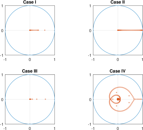
Figure 1: Eigenvalues of the matrix ${\boldsymbol{J}}$ in the complex plane, indicated by red circles, in the four cases of Table 1.

In Figures 2, 3 we observe that in all but one instance the temporal errors always remain below a moderate value and are (essentially) monotonically decreasing as $N$ increases. In Case IV the second adaptation yields large errors for each ADI scheme if $N\lesssim 50$. We attribute this to a lack of unconditional stability, which may reveal itself when $\lambda T$ is large. Except for this instance, for each given adaptation, the MCS scheme with $\theta=\frac{1}{3}$ always yields temporal errors that are smaller than, or approximately equal to, those for the CS and Do schemes, and it always shows a smooth, second-order convergence behaviour. Additional numerical experiments on finer spatial grids, such as with $m_{1}=2m_{2}=400$, show that the temporal errors for all adaptations of the MCS scheme with $\theta=\frac{1}{3}$ are visually identical, indicating that second-order convergence holds in a favourable stiff sense.

In Cases I, II the temporal errors obtained with the CS and Do schemes are often relatively large for $N\lesssim 100$. This is due to the nonsmoothness of the initial function and can be resolved by using backward Euler damping (Rannacher time stepping). This is computationally expensive, however, and does not alter our above conclusion.

Finally, we note that Figures 2, 3 suggest that the temporal error constant increases as $\lambda T$ increases. Additional numerical experiments, where $\lambda$ and $T$ are varied and all else is kept fixed, confirm this.

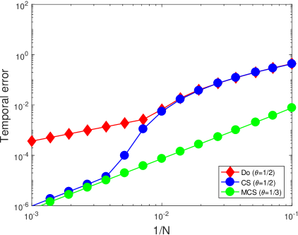
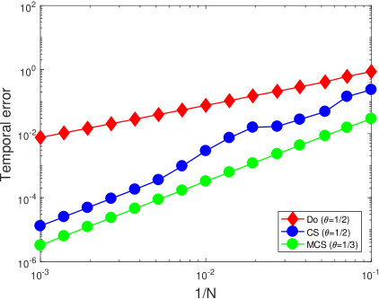
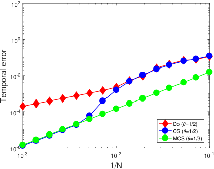
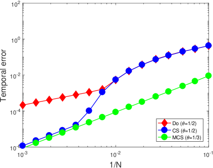
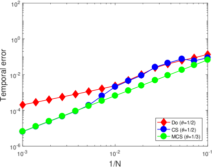
Figure 2: Global temporal errors ${\widehat{e}}\,(N;200,100)$ versus $1/N$. Case I: left column. Case II: right column. Adaptation (3.2): top row. Adaptation (3.3): middle row. Adaptation (3.4): bottom row. ADI schemes: MCS with $\theta=\frac{1}{3}$ (green circles), MCS with $\theta=\frac{1}{2}$ (blue circles) and Do with $\theta=\frac{1}{2}$ (red diamonds).

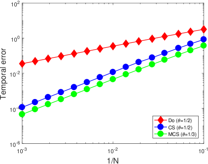
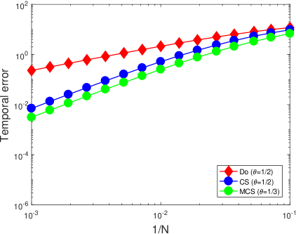
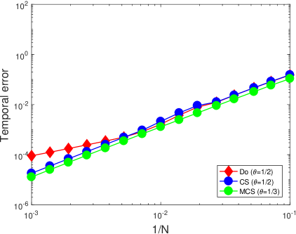
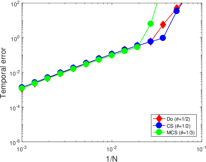
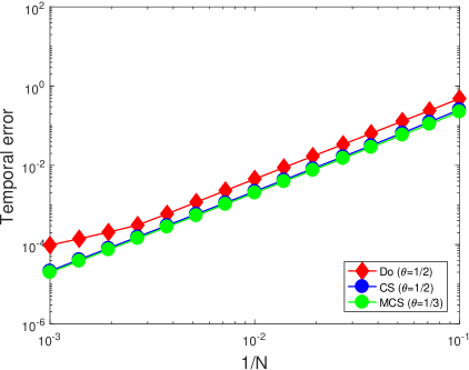
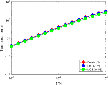
Figure 3: Global temporal errors ${\widehat{e}}\,(N;200,100)$ versus $1/N$. Case III: left column. Case IV: right column. Adaptation (3.2): top row. Adaptation (3.3): middle row. Adaptation (3.4): bottom row. ADI schemes: MCS with $\theta=\frac{1}{3}$ (green circles), MCS with $\theta=\frac{1}{2}$ (blue circles) and Do with $\theta=\frac{1}{2}$ (red diamonds).

5 Conclusion

In this paper we have studied three adaptations of the MCS scheme to two-dimensional PIDEs that are second-order consistent in the classical ODE sense. They treat both the integral term and mixed derivative term explicitly and require per time step the solution of four linear systems with essentially tridiagonal matrices. The first and second adaptations, (3.2) and (3.3), handle the integral term in a one-step fashion and employ two multiplications per time step with the dense matrix corresponding to this term. The third adaptation, (3.4), deals with the integral term in a two-step fashion and uses just one multiplication per time step with the pertinent dense matrix. In view of the stability results obtained in Section 3 and numerical experiments for the Bates PIDE performed in Section 4, we recommend the third adaptation of the MCS scheme with parameter value $\theta=\frac{1}{3}$, directly followed by the first adaptation of this scheme.

References

- [1] A. Almendral and C. W. Oosterlee, Numerical valuation of options with jumps in the underlying, Appl. Numer. Math., 53 (2005), pp. 1–18.
- [2] L. Andersen and J. Andreasen, Jump-diffusion processes: Volatility smile fitting and numerical methods for option pricing, Rev. Deriv. Res., 4 (2000), pp. 231–262.
- [3] A. Arrarás, K. J. in ’t Hout, W. Hundsdorfer, and L. Portero, Modified Douglas splitting methods for reaction-diffusion equations, BIT, 57 (2017), pp. 261–285.
- [4] L. V. Ballestra and L. Cecere, A fast numerical method to price American options under the Bates model, Comput. Math. Appl., 72 (2016), pp. 1305–1319.
- [5] L. V. Ballestra and C. Sgarra, The evaluation of American options in a stochastic volatility model with jumps: an efficient finite element approach, Comput. Math. Appl., 60 (2010), pp. 1571–1590.
- [6] D. S. Bates, Jumps and stochastic volatility: Exchange rate processes implicit in Deutsche Mark options, Rev. Finan. Stud., 9 (1996), pp. 69–107.
- [7] M. Briani, R. Natalini, and G. Russo, Implicit-explicit numerical schemes for jump-diffusion processes, Calcolo, 44 (2007), pp. 33–57.
- [8] C. Chiarella, B. Kang, G. H. Meyer, and A. Ziogas, The evaluation of American option prices under stochastic volatility and jump-diffusion dynamics using the method of lines, Int. J. Theor. Appl. Finan., 12 (2009), pp. 393–425.
- [9] R. Cont and P. Tankov, Financial Modelling with Jump Processes, Chapman & Hall/CRC, Boca Raton, FL, 2004.
- [10] R. Cont and E. Voltchkova, A finite difference scheme for option pricing in jump diffusion and exponential Lévy models, SIAM J. Numer. Anal., 43 (2005), pp. 1596–1626.
- [11] I. J. D. Craig and A. D. Sneyd, An alternating-direction implicit scheme for parabolic equations with mixed derivatives, Comput. Math. Appl., 16 (1988), pp. 341–350.
- [12] Y. d’Halluin, P. A. Forsyth, and K. R. Vetzal, Robust numerical methods for contingent claims under jump diffusion processes, IMA J. Numer. Anal., 25 (2005), pp. 87–112.
- [13] J. Douglas, On the numerical integration of by implicit methods, J. Soc. Ind. Appl. Math., 3 (1955), pp. 42–65.
- [14] J. Douglas and H. H. Rachford, On the numerical solution of heat conduction problems in two and three space variables, Trans. Amer. Math. Soc., 82 (1956), pp. 421–439.
- [15] E. Ekström and J. Tysk, The Black–Scholes equation in stochastic volatility models, J. Math. Anal. Appl., 368 (2010), pp. 498–507.
- [16] L. Feng and V. Linetsky, Pricing options in jump-diffusion models: an extrapolation approach, Oper. Res., 56 (2008), pp. 304–325.
- [17] T. Haentjens and K. J. in ’t Hout, Alternating direction implicit finite difference schemes for the Heston–Hull–White partial differential equation, J. Comput. Finan., 16 (2012), pp. 83–110.
- [18] S. L. Heston, A closed-form solution for options with stochastic volatility with applications to bond and currency options, Rev. Finan. Stud., 6 (1993), pp. 327–343.
- [19] W. Hundsdorfer, Accuracy and stability of splitting with Stabilizing Corrections, Appl. Numer. Math., 42 (2002), pp. 213–233.
- [20] W. Hundsdorfer and J. G. Verwer, Numerical Solution of Time-Dependent Advection-Diffusion-Reaction Equations, vol. 33 of Springer Series in Computational Mathematics, Springer, Berlin, 2003.
- [21] S. Ikonen and J. Toivanen, Efficient numerical methods for pricing American options under stochastic volatility, Numer. Meth. Part. Diff. Eq., 24 (2008), pp. 104–126.
- [22] K. J. in ’t Hout, Numerical Partial Differential Equations in Finance Explained, Financial Engineering Explained, Palgrave Macmillan, London, 2017.
- [23] K. J. in ’t Hout and S. Foulon, ADI finite difference schemes for option pricing in the Heston model with correlation, Int. J. Numer. Anal. Model., 7 (2010), pp. 303–320.
- [24] K. J. in ’t Hout and W. Hundsdorfer, On multistep stabilizing correction splitting methods with applications to the Heston model, arXiv:1709.00622 (2017).
- [25] K. J. in ’t Hout and C. Mishra, Stability of the modified Craig–Sneyd scheme for two-dimensional convection-diffusion equations with mixed derivative term, Math. Comput. Simul., 81 (2011), pp. 2540–2548.
- [26] , Stability of ADI schemes for multidimensional diffusion equations with mixed derivative terms, Appl. Numer. Math., 74 (2013), pp. 83–94.
- [27] K. J. in ’t Hout and J. Toivanen, Application of operator splitting methods in finance, in Splitting Methods in Communication, Imaging, Science, and Engineering, Springer, 2016, pp. 541–575.
- [28] K. J. in ’t Hout and B. D. Welfert, Stability of ADI schemes applied to convection-diffusion equations with mixed derivative terms, Appl. Numer. Math., 57 (2007), pp. 19–35.
- [29] , Unconditional stability of second-order ADI schemes applied to multi-dimensional diffusion equations with mixed derivative terms, Appl. Numer. Math., 59 (2009), pp. 677–692.
- [30] A. Itkin, Pricing Derivatives under Lévy Models, vol. 12 of Pseudo-Differential Operators: Theory and Applications, Birkhäuser, New York, NY, 2017.
- [31] A. Itkin and P. Carr, Jumps without tears: a new splitting technology for barrier options, Int. J. Numer. Anal. Model., 8 (2011), pp. 667–704.
- [32] V. Kaushansky, A. Lipton, and C. Reisinger, Numerical analysis of an extended structural default model with mutual liabilities and jump risk, J. Comp. Sci., to appear (2017).
- [33] Y. Kwon and Y. Lee, A second-order finite difference method for option pricing under jump-diffusion models, SIAM J. Numer. Anal., 49 (2011), pp. 2598–2617.
- [34] S. McKee and A. R. Mitchell, Alternating direction methods for parabolic equations in two space dimensions with a mixed derivative, Computer J., 13 (1970), pp. 81–86.
- [35] S. McKee, D. P. Wall, and S. K. Wilson, An alternating direction implicit scheme for parabolic equations with mixed derivative and convective terms, J. Comput. Phys., 126 (1996), pp. 64–76.
- [36] R. C. Merton, Option pricing when underlying stock returns are discontinuous, J. Finan. Econ., 3 (1976), pp. 125–144.
- [37] C. Mishra, A new stability result for the modified Craig–Sneyd scheme applied to two-dimensional convection-diffusion equations with mixed derivatives, Appl. Math. Comp., 285 (2016), pp. 41–50.
- [38] D. W. Peaceman and H. H. Rachford, The numerical solution of parabolic and elliptic differential equations, J. Soc. Ind. Appl. Math., 3 (1955), pp. 28–41.
- [39] S. Salmi and J. Toivanen, An iterative method for pricing American options under jump-diffusion models, Appl. Numer. Math., 61 (2011), pp. 821–831.
- [40] , IMEX schemes for pricing options under jump-diffusion models, Appl. Numer. Math., 84 (2014), pp. 33–45.
- [41] S. Salmi, J. Toivanen, and L. von Sydow, An IMEX-scheme for pricing options under stochastic volatility models with jumps, SIAM J. Sci. Comput., 36 (2014), pp. B817–B834.
- [42] D. Tavella and C. Randall, Pricing Financial Instruments: The Finite Difference Method, John Wiley & Sons, Chichester, 2000.
- [43] J. Toivanen, A componentwise splitting method for pricing American options under the Bates model, in Applied and Numerical Partial Differential Equations, vol. 15 of Comput. Methods Appl. Sci., Springer, New York, 2010, pp. 213–227.
- [44] L. von Sydow, J. Toivanen, and C. Zhang, Adaptive finite differences and IMEX time-stepping to price options under Bates model, Int. J. Comput. Math., 92 (2015), pp. 2515–2529.