Abstract

In this work, we examine effects of large permanent charges on ionic flow through ion channels based on a quasi-one dimensional Poisson-Nernst-Planck model. It turns out large positive permanent charges inhibit the flux of cation as expected, but strikingly, as the transmembrane electrochemical potential for anion increases in a particular way, the flux of anion decreases. The latter phenomenon was observed experimentally but the cause seemed to be unclear. The mechanisms for these phenomena are examined with the help of the profiles of the ionic concentrations, electric fields and electrochemical potentials. The underlying reasons for the near zero flux of cation and for the decreasing flux of anion are shown to be different over different regions of the permanent charge. Our model is oversimplified. More structural detail and more correlations between ions can and should be included. But the basic finding seems striking and important and deserving of further investigation.

1 Introduction

Membranes define biological cells. They provide the barrier that separates, and defines the inside of a cell from the rest of the world. Membranes are much more than just a barrier. They provide pathways for selected molecules to enter and leave cells. The barriers must not be perfect or cells would soon die from lack of energy or drown in their waste. Biological cells need energy to survive and that is provided (in almost all cases) by substances that must cross the membrane.

Substances cross membranes through proteins specialized for the task. For a very long time ([20, 41]) these proteins have been separated into two classes, channels and transporters ([40]), and studied in two traditions, one of electrophysiology ([18, 46]), the other of enzymology ([19, 36]), although the distinction between the two approaches was less than clearcut ([11]).

Channels have been viewed fundamentally as charged ‘holes in the wall’ (created by the membrane) that could open and close ([35]) but, once open, the channel followed simple laws of electrodiffusion ([8]).

Transporters were viewed as more biological devices, involving conformation changes, coupling to energy sources (either ATP hydrolysis or the movement of other ions), with quantitative description much more difficult, particularly if the description was to be transferrable with parameters that were independent of conditions.

The enormous literature can be sampled in [1, 2, 3, 36, 40]. Structural biology has shown that transporters and channels have very similar structures ([4, 31, 37, 44]). Biophysics has shown that the processes that open and close channels (‘activation’ and ‘inactivation’) can be coupled to give properties rather like transporters. Physics has shown that the electric fields assumed to be constant in classical electrophysiology must depend on the distribution of charge in the channel and surrounding solutions ([9]) and so must change with experimental conditions and with location.

The detailed properties of open channels have not been compared with transporters in the modern literature, as far as we know, certainly not using models that satisfy the physical requirement that potential profiles (i.e., electric fields) be computed from (and thus be consistent with) all the charges in the system.

Here we consider a simple model of a permanently open ion channel. (We leave gating for later consideration.) Most biologists imagine that if the driving force for electrodiffusion is increased–that is to say, if the gradient of electrochemical potential across the channel is increased in magnitude–the flux through the channel should increase. We show here that is not always the case. Consider a channel with large permanent charge and the flux of ions with the opposite sign as the permanent charge (called counter ions in the ion exchange literature ([17]) or majority charge carriers in the semiconductor literature ([34, 38, 43]). The flux of ions with the opposite sign as the permanent charge in a channel can decrease dramatically as the driving force increases – we term this phenomenon as the declining phenomenon. More precisely, if the concentration of the ion is held fixed on one side of the channel, and the concentration decreased on the other (‘trans’) side of the channel, the flux of the counter ions can decrease if the permanent charge density is large, as we show here. A depletion zone can form that prevents flow even though the driving force increases to large values. It is worthwhile to emphasize that if one increases the transmembrane electrochemical potential in a different manner, such as, by increasing the transmembrane electric potential or the concentration of the ion at one side of the channel, then one does not have the declining phenomenon (see Remark 5.1).

The decline of flux with trans concentration has been considered a particular, even defining proerties of transporters, involving conformation changes of state and other properties of proteins less well defined (physically) than electrodiffusion ([24, 42]). Declining flux has been called exchange diffusion (in the early transport literature) and self-exchange more recently and is an example of obligatory exchange. Obligatory exchange is a wide spread, nearly universal property of the nearly eight hundred transporters known twenty years ago ([1, 16]) with many more known today ([39]). Obligatory exchange is ascribed widely to changes in the structure of transport proteins, to conformation changes in the spatial distribution of the mass of the protein ([14]). Obligatory exchange is often thought to be a special property of transporters not found in channels.

The structure of many transporters is now known thanks to the remarkable advances of cryo-electron microscopy, recognized in the 2018 Nobel Prize. A transporter (of one amino acid sequence and thus of a perfectly homogeneous molecular type) exists in different states. Each state is said to have a different conformation meaning, in physical language, that the spatial distribution of mass is different in different states, and the distributions of the different states form disjoint sets, with no overlap. The movement of ions is not directly controlled or driven by the conformation of mass, however. Rather the distribution of mass produces a distribution of steric repulsion forces, and a spatial distribution of electrical forces (because the mass is associated with charge, mostly permanent charge of acid and base groups of the protein, but also significant polarization charge, as well). It is the conformation of these forces that determines the movement of ions. The spatial distribution of forces contributes to the potential of mean force reported in simulations of molecular dynamics.

This paper shows that channels with one spatial distribution of mass can have properties of self-exchange (for majority charge carrier counter ions) if the density of permanent charge is large. The spatial distribution of electrical forces can change and create a depletion zone that controls ion movement, while the spatial distribution of the mass of the protein does not change. The conformation governing current flow is the conformation of the electric field – the depletion zone – more than the conformation of mass, in the model considered here. The current flow of counter ions is much greater than the current flow of co-ions because there are many more counter ions than co-ions near the permanent charge. Transporters almost always allow much less current flow than channels.

It should be emphasized that the depletion zone considered here arises from the self-consistent solution of the Poisson-Nernst-Planck (PNP) equations of a specific model (large permanent charge, counter ion transport) and that parameters are not adjusted in any way to create or modify the phenomena. This is in stark contrast to calculations of chemical kinetic models that involve many adjustable parameters, without clear physical meaning, and equations that do not conserve current ([6]).

Depletion zones play crucial roles in the behavior of nonlinear semiconductor devices although there they usually arise at locations in PN diodes where permanent charge (called doping in that literature) changes sign. Depletion zones of the type studied here are likely to occur in semiconductors but have received little attention because they have less dramatic effects than those in diodes ([34, 38, 43]) that follow drift diffusion and PNP equations rather like those of open ionic channels ([7, 9]). The possible role of depletion zones in channel function has been the source of speculation and experimental verification ([10, 32]). It is striking that depletion zones can change the conformation of the electric field and mimic the obligatory exchange traditionally thought to occur only in transporters. Depletion zones can create plastic electric fields whose change in shape dominate the flux through a channel of fixed structure.

Our model is of course oversimplified as are any models, or even simulations in apparent atomic detail, of condensed phases. More structural detail and more correlations between ions can and should be included. But the basic finding that large permanent charge can produce depletion zones and those regions can produce a decline of counter ion flux when driving forces increase seems striking and important and deserving of further investigation.

The rest of the paper is organized as follows. In Section 2, we describe the quasi-one-dimensional Poisson-Nernst-Planck type model and its dimensionless form for ionic flow. Assumptions are specified with two key assumptions: a dimensionless parameter $\varepsilon$ defined in (2.9) is small and a dimensionless parameter $Q_{0}>0$ defined in (2.12) from the permanent charge is large. In Section 3, approximation formulas (in small $\varepsilon$ and $\nu=1/{Q_{0}}$) for fluxes are provided, which have a number of non-trivial consequences. One of the apparent non-trivial consequences is that the leading order term $J_{10}$ of cation flux is zero, independent of the values of transmembrane electrochemical potential of the cation. The mechanism of this distinguished effect of large (positive) permanent charge is examined in details in Section 4 with the help of the internal dynamics (profiles of the electric field, cation concentrations and electrochemical potential). It turns out the mechanism for $J_{10}=0$ is different over different regions of permanent charge. In Section 5, a rather counter-intuitive declining phenomenon – increasing of anion transmembrane electrochemical potential leads to decreasing of anion flux – is shown to be consistent with our analytical result. Thus, for the first time (to the best of our knowledge), a mechanism of large permanent charge for such a phenomenon is revealed. The mechanism is then examined in details again with the help of the internal dynamics. We conclude this paper with a general remark in Section 6.

2 Classical PNP with large (positive) permanent charge

2.1 A quasi-one-dimensional PNP model

Our study is based on a quasi-one-dimensional PNP model for open channels, first proposed in [33] and, for a special case, rigorously justified in [28]. For a mixture of $n$ ion species, a quasi-one-dimensional PNP model is

$$\begin{split}&\frac{1}{A(X)}\frac{d}{dX}\Big{(}\varepsilon_{r}(X)\varepsilon_{0}A(X)\frac{d\Phi}{dX}\Big{)}=-e_{0}\Big{(}\sum_{s=1}^{n}z_{s}C_{s}+{\cal Q}(X)\Big{)},\\ &\frac{d{\cal J}_{k}}{dX}=0,\quad-{\cal J}_{k}=\frac{1}{k_{B}T}{\cal D}_{k}(X)A(X)C_{k}\frac{d\mu_{k}}{dX},\quad k=1,2,\cdots,n\end{split}$$ (2.1)

where $X\in[a_{0},b_{0}]$ is the coordinate along the axis of the channel and baths, $A(X)$ is the cross-sectional area of the channel at the location $X$, $e_{0}$ is the elementary charge, $\varepsilon_{0}$ is the vacuum permittivity, $\varepsilon_{r}(X)$ is the relative dielectric coefficient, ${\cal Q}(X)$ is the permanent charge density, $k_{B}$ is the Boltzmann constant, $T$ is the absolute temperature, $\Phi$ is the electrical potential, and, for the $k$th ion species, $C_{k}$ is the concentration, $z_{k}$ is the valence, ${\cal D}_{k}(X)$ is the diffusion coefficient, $\mu_{k}$ is the electrochemical potential, and ${\cal J}_{k}$ is the flux density.

Equipped with system (LABEL:ssPNP), a meaningful boundary condition for ionic flow through ion channels (see, [12] for a reasoning) is, for $k=1,2,\cdots,n$,

$$\Phi(a_{0})={\cal V},\ \ C_{k}(a_{0})={\cal L}_{k}>0;\quad\Phi(b_{0})=0,\ \ C_{k}(b_{0})={\cal R}_{k}>0.$$ (2.2)

Mathematically, we will be interested in solutions of the boundary value problem (BVP) (LABEL:ssPNP) and (2.2). An important measurement for properties of ion channels is the I-V (current-voltage) relation where the current ${\cal I}$ depends on the transmembrane potential (voltage) ${\cal V}$ and is given by

$${\cal I}=\sum_{s=1}^{n}z_{s}{\cal J}_{s}({\cal V})$$

where ${\cal J}_{k}({\cal V})$’s are determined by the BVP (LABEL:ssPNP) and (2.2) for fixed ${\cal L}_{k}$’s and ${\cal R}_{k}$’s. Of course, the relations of individual fluxes ${\cal J}_{k}$’s to ${\cal V}$ contain more information ([21]) but it is much harder to experimentally measure the individual fluxes ${\cal J}_{k}$’s.

2.1.1 Electroneutrality boundary conditions

In relation to typical experimental designs, the positions $X=a_{0}$ and $X=b_{0}$ are located in the baths separated by the channel. They are the locations of two electrodes that are applied to control or drive the ionic flow through the ion channel. Ideally, the experimental designs should not affect the intrinsic ionic flow properties so one would like to design the boundary conditions to meet the so-called electroneutrality

$$\sum_{s=1}^{n}z_{s}{\cal L}_{s}=0=\sum_{s=1}^{n}z_{s}{\cal R}_{s}.$$ (2.3)

The reason for this is that, otherwise, there will be sharp boundary layers which cause significant changes (large gradients) of the electric potential and concentrations near the boundaries so that a measurement of these values has non-trivial uncertainties. One clever design to remedy this potential problem is the “four-electrode-design”: two “outer-electrodes” in the baths far away from the ends of the ion channel to provide the driving force and two “inner-electrodes” in the baths near the ends of the ion channel to measure the electrical potential and the concentrations as the “real” boundary conditions for the ionic flow. At the inner electrodes locations, the electroneutrality conditions are reasonably satisfied, and hence, the electric potential and concentrations vary slowly and a measurement of these values would be robust. We point out that the geometric singular perturbation framework for PNP type models developed in [12, 13, 22, 25, 26, 27] can treat the case without electroneutrality assumption; in fact, the boundary layers can be determined by the boundary conditions directly.

2.1.2 Electrochemical potentials

The electrochemical potentials $\mu_{k}(X)$ consists of the ideal component $\mu_{k}^{id}$ and the excess component $\mu_{k}^{ex}$ where the ideal component

$$\mu_{k}^{id}(X)=z_{k}e_{0}\Phi(X)+k_{B}T\ln\frac{C_{k}(X)}{C_{0}}$$ (2.4)

is the point-charge contribution where $C_{0}$ is a characteristic concentration, and the excess component $\mu_{k}^{ex}(x)$ accounts for ion size effects. As explained above, although not totally physical for ion channel problems in general, we will consider only the ideal component in this work that can act as guidance for further studies of more accurate models with excess component.

2.1.3 Permanent charges and channel geometry

The permanent charge ${\cal Q}(X)$ is a simplified mathematical model for ion channel (protein) structure. It is determined by the spatial distribution of amino acids in the channel wall, the acid (negative) and base (positive) side chains, more than anything else ([9]). We will assume ${\cal Q}(X)$ is known and take an oversimplified description to capture some essence of its effects. For this paper, we take it to be as in ([12]), for some $a_{0}<A<B<b_{0}$,

$${\cal Q}(X)=\left\{\begin{array}[]{cc}0,&X\in[a_{0},A)\cup(B,b_{0}]\\ 2{\cal Q}_{0},&X\in(A,B).\end{array}\right.$$ (2.7)

We will be interested in the case where $|{\cal Q}_{0}|$ is large relative to ${\cal L}_{k}$’s and ${\cal R}_{k}$’s.

The cross-sectional area $A(X)$ typically has the property that $A(X)$ is much smaller for $X\in(A,B)$ (the neck region) than that for $X\not\in(A,B)$. It is interesting to note that, in [23], the authors showed that the neck of the channel should be “narrow” (small $A(X)$ for $X\in(A,B)$) and “short” (small $B-A$) to optimize an effect of permanent charge.

2.1.4 Dielectric coefficient and diffusion coefficients

We assume that

$$\varepsilon(X)=\varepsilon_{r}\,\mbox{ is a constant, and }\;{\cal D}_{k}(X)={\cal D}(X){\cal D}_{k}$$ (2.8)

for some dimensionless function ${\cal D}(X)$ (same for all $k$) and dimensional constant ${\cal D}_{k}$.

Note that the assumption ${\cal D}_{k}(X)={\cal D}(X){\cal D}_{k}$ is equivalent to the statement that ${\cal D}_{k}(X)/{{\cal D}_{j}(X)}$ is a constant for $k\neq j$. Roughly speaking, the assumption says that, as the environment varies from location to location, its influences on the two diffusion coefficients ${\cal D}_{k}(X)$ and ${\cal D}_{j}(X)$ at the same location $x$ are the same; that is, the two diffusion coefficients vary from one common environment to another common environment in a way so that their ratio is independent of locations. This is not a justification of this assumption but only an explanation of what it reflects.

2.1.5 Main assumptions

In the sequel, we assume the boundary electroneutrality condition in (2.3), the form of the permanent charge in (2.7), constant dielectric coefficient and diffusion coefficient property in (2.8), and the electrochemical potential is ideal $\mu_{k}=\mu_{k}^{id}$ in (2.4). There are two key assumptions for this work to be discussed in terms of dimensionless variables below.

2.2 Dimensionless form of the quasi-one-dimensional PNP model

The following rescaling (see [15]) or its variations have been widely used for convenience of mathematical analysis.

Let $C_{0}$ be a characteristic concentration of the ion solution. We now make a dimensionless re-scaling of the variables in system (LABEL:ssPNP) as follows.

$$\begin{split}&\varepsilon^{2}=\frac{\varepsilon_{r}\varepsilon_{0}k_{B}T}{e_{0}^{2}(b_{0}-a_{0})^{2}C_{0}},\;x=\frac{X-a_{0}}{b_{0}-a_{0}},\;h(x)=\frac{A(X)}{(b_{0}-a_{0})^{2}},\;Q(x)=\frac{{\cal Q}(X)}{C_{0}},\\ &D(x)={\cal D}(X),\;\phi(x)=\frac{e_{0}}{k_{B}T}\Phi(X),\;c_{k}(x)=\frac{C_{k}(X)}{C_{0}},\;J_{k}=\frac{{\cal J}_{k}}{(b_{0}-a_{0})C_{0}{\cal D}_{k}}.\end{split}$$ (2.9)

The dimensionless quantity $Q(x)$ from the permanent charge ${\cal Q}$ in (2.7) becomes

$$Q(x)=\left\{\begin{array}[]{cc}0,&x\in[0,a)\cup(b,1]\\ 2Q_{0},&x\in(a,b),\end{array}\right.$$ (2.12)

where

$$0<a=\frac{A-a_{0}}{b_{0}-a_{0}}<b=\frac{B-a_{0}}{b_{0}-a_{0}}<1,$$

and, in terms of the dimensionless quantities, the subinterval $(a,b)\subset(0,1)$ corresponds to the neck region $[A,B]$.

Key assumptions. The parameter $\varepsilon$ is small and the parameter $Q_{0}>0$ is large.

The case where $Q_{0}<0$ with $|Q_{0}|$ large can be treated in the same way. The assumption of smallness of the dimensionless parameter $\varepsilon$ is reasonable particularly because we are interested in the limit of large $|Q_{0}|$. Thus, we can take large but fixed characteristic concentration $C_{0}$ in the definition of $\varepsilon$ (2.9). For example, if $b_{0}-a_{0}=25nm$ and $C_{0}=10M$, then the dimensionless parameter $\varepsilon\approx 10^{-3}$ ([5]). The mathematical consequence of smallness of $\varepsilon$ is that the BVP (2.13) and (2.14) can be treated as a singularly perturbed problem. A general geometric framework for analyzing the singularly perturbed BVP of PNP type systems has been developed in [12, 26, 27, 30] for classical PNP systems and in [22, 25, 29] for PNP systems with finite ion sizes.

In terms of the new variables in (2.9), the BVP (LABEL:ssPNP) and (2.2) becomes

$$\begin{split}&\frac{\varepsilon^{2}}{h(x)}\frac{d}{dx}\left(h(x)\frac{d\phi}{dx}\right)=-\sum_{s=1}^{n}z_{s}c_{s}-Q(x),\\ &\frac{dJ_{k}}{dx}=0,\quad-J_{k}=\frac{1}{k_{B}T}D(x)h(x)c_{k}\frac{d\mu_{k}}{dx},\end{split}$$ (2.13)

with boundary conditions at $x=0$ and $x=1$

$$\begin{split}\phi(0)=&V,\;c_{k}(0)=L_{k};\;\phi(1)=0,\;c_{k}(1)=R_{k},\end{split}$$ (2.14)

where

$$V:=\frac{e_{0}}{k_{B}T}{\cal V},\quad L_{k}:=\frac{{\cal L}_{k}}{C_{0}},\quad R_{k}:=\frac{{\cal R}_{k}}{C_{0}}.$$

In this work, we will consider the BVP (2.13) and (2.14) for ionic mixtures with one cation of valence $z_{1}=1$ and an anion of valence $z_{2}=-1$. We will be interested in properties of ionic flow for large $|Q_{0}|$. It turns out

$$\alpha=\frac{H(a)}{H(1)}\;\mbox{ and }\;\beta=\frac{H(b)}{H(1)}\;\;\mbox{ where }\;H(x)=\int_{0}^{x}\frac{1}{D(s)h(s)}ds$$

are the key parameters that characterize the effect of channel geometry and location of permanent charge. The physical meanings of these parameters could be seen from the special case when $h(x)=h_{0}$ and $D(x)=D_{0}$ are constants. In this case,

$$H(x)=\frac{x}{D_{0}h_{0}},$$

which is proportional to the (scaled) length $x$ of the region over $[0,x]$ of the channel (conductive material), inversely proportional to the (scaled) cross-sectional area $h_{0}$ of the channel and to the (scaled) diffusion coefficient or electric conductivity $D_{0}$; that is, $H(x)$ is the resistance of the portion of the channel over $[0,x]$.

3 Approximations of fluxes [45].

We now recall the results on approximations of $(\phi,c_{1},c_{2},J_{1},J_{2})$ and $\mu_{k}$’s from [45] for the case where $z_{1}=1$ and $z_{2}=-1$ with $L_{1}=L_{2}=L$ and $R_{1}=R_{2}=R$.

Based on the assumptions that $\varepsilon>0$ is SMALL and $Q_{0}>0$ is LARGE, one has expansions of fluxes in $\varepsilon$ and in $\nu=1/{Q_{0}}$ near $\varepsilon=0$ and $\nu=0$.

First, one expands the fluxes in $\varepsilon$ as

$$J_{1}(\varepsilon;\nu)=J_{1}(\nu)+O(\varepsilon)\;\mbox{ and }\;J_{2}(\varepsilon)=J_{2}(\nu)+O(\varepsilon),$$

where $J_{k}(\nu)$, depending also on the parameters $(V,L,R,H(1),\alpha,\beta)$, are the zeroth order in $\varepsilon$ terms of the fluxes. Then, one expands $J_{k}(\nu)$ about $\nu$ as

$$J_{1}(\nu)=J_{10}+J_{11}\nu+O(\nu^{2})\;\mbox{ and }\;J_{2}(\nu)=J_{20}+J_{21}\nu+O(\nu^{2}).$$

Thus,

$$J_{1}(\varepsilon;\nu)=J_{10}+J_{11}\nu+O(\nu^{2},\varepsilon)\;\mbox{ and }\;J_{2}(\varepsilon;\nu)=J_{20}+J_{21}\nu+O(\nu^{2},\varepsilon).$$ (3.1)

Note that $J_{10}$ and $J_{20}$, depending on $(V,L,R,H(1),\alpha,\beta)$, contain the leading order effect of the small $\nu$ (or equivalently, large $Q_{0}$).

The following result is established in [45].

Proposition 3.1.

One has

$$\begin{split}J_{10}&=0,\\ J_{11}&=\frac{1}{2H(1)(\beta-\alpha)}\left(\frac{(1-\beta)L+\alpha R}{(1-\beta)\sqrt{e^{V}L}+\alpha\sqrt{R}}\right)^{2}(e^{V}L-R);\\ J_{20}&=\frac{2\sqrt{LR}}{H(1)}\frac{1}{(1-\beta)\sqrt{L}+\alpha\sqrt{e^{-V}R}}(\sqrt{e^{-V}L}-\sqrt{R}),\\ J_{21}&=\frac{(1-\beta)L+\alpha R}{2H(1)(\beta-\alpha)(\sqrt{e^{-V}L}-\sqrt{R})((1-\beta)\sqrt{L}+\alpha\sqrt{e^{-V}R})^{3}}\\ &\quad\left\{-2(\beta-\alpha)^{2}(\sqrt{e^{-V}L}-\sqrt{R})^{2}\sqrt{e^{-V}}LR\right.\\ &\quad\left.+((1-\beta)L+\alpha R)(L-Re^{-V})\left[\frac{(1-\beta)L+\alpha R}{2}\sqrt{e^{-V}}\ln{\frac{L}{e^{V}R}}\right.\right.\\ &\qquad\qquad\left.\left.-((1-\beta)\sqrt{L}+\alpha\sqrt{e^{-V}R})(\sqrt{e^{-V}L}-\sqrt{R})\right]\right\}.\end{split}$$ (3.2)

A distinct implication of $J_{10}=0$ in Proposition 3.1 is that large (positive) permanent charge $Q_{0}$ (or small $\nu=1/{Q_{0}}$) inhibits the cation flux. We will provide a detailed discussion in Section 4 on what happens to the internal dynamics that is consistent with this conclusion.

To this end, we recall another immediate consequence of (3.2) (see [45] for more).

Corollary 3.2.

[Current Saturation] For large permanent charge $Q_{0}$ (small ${\nu}=1/{Q_{0}}$) and to the leading order terms in $\nu$, each individual fluxes $J_{k}$’s, and hence, the total current $I$ saturate as $|V|\to\infty$; more precisely, one has

$$\begin{split}\lim_{V\to+\infty}J_{20}=&-\frac{1}{1-\beta}\frac{2R}{H(1)},\quad\lim_{V\to-\infty}J_{20}=\frac{1}{\alpha}\frac{2L}{H(1)},\\ \lim_{V\to+\infty}J_{11}=&-\lim_{V\to+\infty}J_{21}=\frac{1}{(1-\beta)^{2}}\frac{((1-\beta)L+\alpha R)^{2}}{2H(1)(\beta-\alpha)},\\ \lim_{V\to-\infty}J_{11}=&-\lim_{V\to-\infty}J_{21}=-\frac{1}{\alpha^{2}}\frac{((1-\beta)L+\alpha R)^{2}}{2H(1)(\beta-\alpha)}.\end{split}$$ (3.3)

Proof.

All the above (finite) limits can be derived from (3.2) easily. ∎

Note this is NOT the case if the permanent charge is small ([23]).

4 Internal dynamics for $J_{10}=0$.

It follows from the Nernst-Planck equation in (2.13) that

$$J_{1}\int_{0}^{1}\frac{k_{B}T}{D_{1}(x)h(x)c_{1}(x)}dx=\mu_{1}(0)-\mu_{1}(1).$$

Thus, $J_{1}$ has the same sign as that of $\mu_{1}(0)-\mu_{1}(1)$; in particular, if $\mu_{1}(0)-\mu_{1}(1)\neq 0$, then $J_{1}\neq 0$.

For the setup of this paper, there are three regions of permanent charge $Q(x)$: $Q(x)=0$ for $x\in[0,a)$ and $x\in(b,1]$ and $Q(x)=2Q_{0}$ for $x\in[a,b]$ with large $Q_{0}$ or small $\nu$ with ${\nu}=1/{Q_{0}}$. A major consequence of large $Q_{0}$ is, from Proposition 3.1, up to the leading order in $\nu=1/{Q_{0}}$ and in $\varepsilon$, the flux of cation is $J_{10}=0$, even if the transmembrane potential $\mu_{1}(0)-\mu_{1}(1)\neq 0$. We will reveal the internal dynamics that lead to this conclusion. To do so, we will discuss what happens over each subinterval based on the approximated (of zeroth order in $\varepsilon$) functions of profiles. Let

$$(\phi(x;\varepsilon,\nu),c_{k}(x;\varepsilon,\nu),J_{k}(\varepsilon,\nu))=(\phi(x;\nu),c_{k}(x;\nu),J_{k}(\nu))+O(\varepsilon)$$ (4.1)

be the solution of the BVP (2.13) and (2.14). For $\nu>0$ small, one has the following expansions

$$J_{1}(\nu)= J_{10}+J_{11}\nu+O(\nu^{2}),$$

where $J_{10}=0$ and $J_{11}$ are given in (3.2). We will also provide figures for the profiles of rescaled electrical potential $\phi(x;\nu)$, cation concentration $c_{1}(x;\nu)$ and electrochemical potential $\mu_{1}(x;\nu)$ of cation, respectively. The parameter values used are

$$\begin{split}e_{0}=&1.6022\times 10^{-19}\ (C),\ k_{B}=1.3806\times 10^{-23}\ (JK^{-1}),\ T=273.16\ (K),\\ \mathcal{V}=&0.01\ (V),\ {\cal L}=0.5\ (M),\;{\cal R}=10^{-5}\ (M),\;{\cal Q}_{0}=10^{8}\ (M),\;C_{0}=1\ (M),\\ a_{0}=&0,\;b_{0}=10\ (nm),\;A=1/3\ (nm),\;B=1/2\ (nm).\end{split}$$ (4.2)

In terms of the dimensionless parameters,

$$V\approx 0.425,\;L=0.5,\;R=10^{-5}\approx 0,\;\;a=\frac{1}{3},\;b=\frac{1}{2},\;\ \nu=10^{-8}\approx 0,$$

The scaled cross-sectional area $h(x)$ is taken to be

$$h(x)=\left\{\begin{array}[]{ccc}\pi(-x+r_{0}+a)^{2},&x\in(0,a)\\ \pi r_{0}^{2},&x\in(a,b)\\ \pi(x+r_{0}-b)^{2},&x\in(b,1).\end{array}\right.$$

The same setup will be used for figures in Section 5.

Notice that the whole interval is $(0,1)$, and it is divided into three subintervals $(0,a),(a,b)$ and $(b,1)$. Permanent charge is located over $(a,b)$. The radius of the neck of ion channel is $c$. In the figures, we let $r_{0}=0.5$. We make plots of each function in interval $(0,1)$, also in every subintervals.

4.1 Internal dynamics over the interval $(0,a)$

The leading order terms of $(\phi,c_{1})$ in (4.1) are derived in [45]. One has

Proposition 4.1.

For $x\in(0,a)$,

$$\phi(x;\nu)= \phi_{0}(x)+\phi_{1}(x)\nu+O(\nu^{2})\mbox{ with }$$

$$\phi_{0}(x)= V-\ln\Big{(}1-\frac{J_{20}}{2L}H(x)\Big{)},\quad\phi_{1}(x)=-\frac{c_{11}(x)}{c_{10}(x)}+\frac{2J_{11}}{J_{20}}\ln{\frac{c_{10}(x)}{L}};$$

$$c_{10}(x)= L-\frac{J_{20}}{2}H(x),\quad c_{11}(x)=-\frac{J_{11}+J_{21}}{2}H(x);$$

$$\mu_{10}(x)= \mu_{10}(0)=V+\ln{L},\quad\mu_{11}(x)=2\frac{J_{11}}{J_{20}}\ln{\frac{c_{10}(x)}{L}}.$$

Figure 1 shows the profiles of $c_{1}(x;\nu)$, $\phi(x;\nu)$ and $\mu_{1}(x;\nu)$ over the interval $(0,a)$.

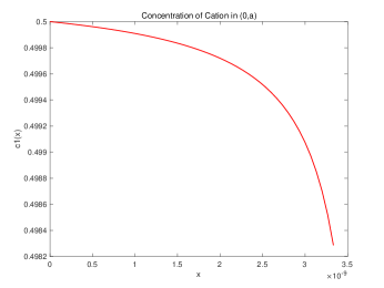
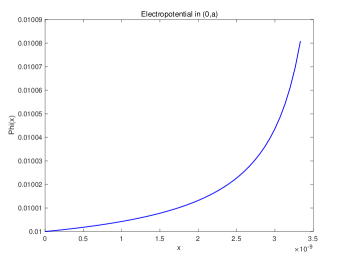
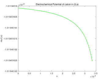
Figure 1: Profiles of $c_{1}(x;\nu)$, $\phi(x;\nu)$, and $\mu_{1}(x;\nu)$ over interval $[0,a]$. Note that $\mu_{10}^{\prime}(x)=0$ but $\mu_{1}^{\prime}(x;\nu)=\mu_{11}^{\prime}(x)\nu+O(\nu^{2})\neq 0$ as shown in the figure.

The following is then a direct consequence.

Corollary 4.2.

Over the interval $(0,a)$, $c_{10}(x)=O(1)$ and $\mu_{10}^{\prime}(x)=0$, and hence, one has $J_{10}=0$.

4.2 Internal dynamics over the interval $(a,b)$

It follows again from [45] that one has the following approximations.

Proposition 4.3.

For $x\in(a,b)$,

$$\phi(x;\nu)= -\ln\nu+\phi_{0}(x)+\phi_{1}(x)\nu+O(\nu^{2})\;\mbox{ with }$$

$$\phi_{0}(x)= \ln{R}-2\ln{B_{0}}+\ln{2},$$

$$\phi_{1}(x)= \phi_{1}^{a}-A_{0}+\frac{J_{20}}{2}(H(x)-H(a));$$

$$c_{10}(x)= 0,\quad c_{11}(x)=\frac{1}{2}A_{0}^{2}-J_{11}(H(x)-H(a)),$$

$$\mu_{10}(x)= \ln{R}-2\ln{B_{0}}+\ln{2}+\ln{\left(\frac{1}{2}A_{0}^{2}-J_{11}(H(x)-H(a))\right)},$$

$$\mu_{11}(x)= \phi_{1}^{a}-A_{0}+\frac{J_{20}}{2}(H(x)-H(a)),$$

where

$$A_{0}= \frac{\sqrt{e^{V}L}}{(1-\beta)\sqrt{e^{V}L}+\alpha\sqrt{R}}((1-\beta)L+\alpha R),$$

$$B_{0}= \frac{\sqrt{R}}{(1-\beta)\sqrt{e^{V}L}+\alpha\sqrt{R}}((1-\beta)L+\alpha R),$$

$$A_{1}= \frac{2(\beta-\alpha)^{2}(L-A_{0})^{2}-\alpha^{2}(A_{0}^{2}-B_{0}^{2})\ln{\frac{B_{0}L}{A_{0}R}}}{4(\beta-\alpha)((1-\beta)L+\alpha R)(L-A_{0})}A_{0}B_{0},$$

$$B_{1}= -\frac{(1-\beta)\left(2(\beta-\alpha)^{2}(L-A_{0})^{2}-\alpha^{2}(A_{0}^{2}-B_{0}^{2})\ln{\frac{B_{0}L}{A_{0}R}}\right)}{4\alpha(\beta-\alpha)((1-\beta)L+\alpha R)(L-A_{0})}A_{0}B_{0},$$

$$\phi_{1}^{a}= \frac{\ln{\frac{B_{0}}{R}}}{\ln{\frac{B_{0}L}{A_{0}R}}}\left(2\Big{(}\frac{B_{1}}{B_{0}}-\frac{A_{1}}{A_{0}}\Big{)}+\frac{\beta-\alpha}{\alpha}(L-A_{0})\right)-2\frac{B_{1}}{B_{0}}-\frac{\beta}{\alpha}(L-A_{0})+L.$$

Figure 2 includes the profiles of $c_{1}(x;\nu)$, $\phi(x;\nu)$, and $\mu_{1}(x;\nu)$ over interval $[a,b]$.

One has the following immediate consequence.

Corollary 4.4.

Over the interval $(a,b)$, $c_{10}(x)=0$, and hence, $J_{10}=0$. Furthermore, $\mu_{10}(a)=V+\ln L$ and $\mu_{10}(b)=\ln R$. As $R\to 0$, $\mu_{10}(a)-\mu_{10}(b)\to\infty$.

Proof.

It follows from Proposition 4.3 directly. ∎

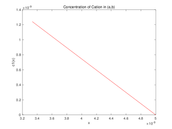
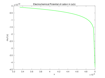
Figure 2: Profiles of $c_{1}(x;\nu)$, $\phi(x;\nu)$, $\mu_{1}(x;\nu)$ over interval $[a,b]$. Note that $c_{10}(x)=0$ but $c_{1}(x;\nu)=c_{10}(x)+c_{11}(x)\nu+O(\nu^{2})=c_{11}(x)\nu+O(\nu^{2})\neq 0$ as shown in the figure. Also note the large drop of $\mu_{1}(x)$ over this interval due to that $R$ is taken to be small.

4.3 Internal dynamics over the interval $(b,1)$

Proposition 4.5.

For $x\in(b,1)$,

$$\phi(x;\nu)= \phi_{0}(x)+\phi_{1}(x)\nu+O(\nu^{2})\;\mbox{ with }$$

$$\phi_{0}(x)= \ln R-\ln c_{10}(x),$$

$$\phi_{1}(x)= \phi_{1}^{b}-\frac{1}{2}\left(B_{0}^{2}-\frac{2B_{1}-B_{0}^{2}}{B_{0}}\right)-\frac{B_{0}c_{11}(x)-B_{1}c_{10}(x)}{B_{0}c_{10}(x)}+\frac{2J_{11}}{J_{20}}\ln{\frac{c_{10}(x)}{B_{0}}};$$

$$c_{10}(x)= B_{0}-\frac{J_{20}}{2}(H(x)-H(b)),\quad c_{11}(x)=B_{1}-\frac{J_{11}+J_{21}}{2}(H(x)-H(b));$$

$$\mu_{10}(x)= \mu_{10}(1)=\ln{R},\quad\mu_{11}(x)=\phi_{1}(x)+\frac{c_{11}(x)}{c_{10}(x)},$$

where

$$\phi_{1}^{b}= \frac{\ln{\frac{B_{0}}{R}}}{\ln{\frac{B_{0}L}{A_{0}R}}}\left(2\Big{(}\frac{B_{1}}{B_{0}}-\frac{A_{1}}{A_{0}}\Big{)}+\frac{\beta-\alpha}{\alpha}(L-A_{0})\right)-2\frac{B_{1}}{B_{0}}+B_{0}.$$

Figure 3 shows the profiles of $c_{1}(x;\nu)$, $\phi(x;\nu)$, and $\mu_{1}(x;\nu)$ over interval $[b,1]$.

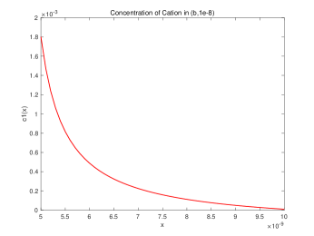
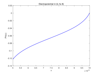
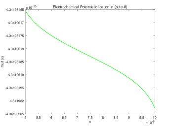
Figure 3: Profiles of $c_{1}(x;\nu)$, $\phi(x;\nu)$, and $\mu_{1}(x;\nu)$ on interval $[b,1]$. Note that $\mu_{10}^{\prime}(x)=0$ but $\mu_{1}^{\prime}(x;\nu)=\mu_{10}(x)+\mu_{11}^{\prime}(x)\nu+O(\nu^{2})=\mu_{11}^{\prime}(x)\nu+O(\nu^{2})\neq 0$.

Corollary 4.6.

Over the interval $(b,1)$, noting $B_{0}=O(\sqrt{R})$, $c_{10}(x)=O(1)$ and $\mu_{1}^{\prime}(x)=0$, and hence, $J_{10}=0$.

4.4 Summary of mechanism for $J_{10}=0$.

From the above discussion, we conclude that the mechanisms for $J_{10}=0$ are different over each subintervals. More precisely, one has that,

• over the first interval $(0,a)$, $J_{10}=0$ is the result of constant electrochemical potential $\mu_{10}(x)=\mu_{10}(0)=\mu_{10}(a)$ (so that $\mu_{10}^{\prime}(x)=0$) while $c_{10}(x)\neq 0$;

• over the last interval $(b,1)$, similar to that over the first interval $(0,a)$, $\mu_{10}(x)=\mu_{10}(1)$ so that $\mu_{10}^{\prime}(x)=0$ while $c_{10}(x)\neq 0$, and, for $R$ small, $c_{10}(x)=O(\sqrt{R})$ over this interval;

• over the middle interval $(a,b)$ where permanent charge is not zero and large, the electrochemical potential $\mu_{10}(x)$ is not a constant so that $\mu_{10}^{\prime}(x)\neq 0$, however, $c_{10}(x)=0$, in particular, the drop of $\mu_{10}(x)$ over this interval equals the transmembrane electrochemical potentials, that is, $\mu_{10}(a)-\mu_{10}(b)=\mu_{1}(0)-\mu_{1}(1)$.

Here we provide the profiles of concentration (Fig. 4), electrical potential (Fig. 5) and electrochemical potential (Fig. 6) over the whole interval $[0,1]$.

The figures of $c_{1}(x)$ and $\phi(x)$ over interval $(0,x_{0})$ are not continue, because we make the plots of system (LABEL:ssPNP) with $\varepsilon=0$. For the limiting system at $x=a$ and $x=b$, there are two fast layers, $c_{1}(x)$ and $\phi(x)$ changes very fast, but $\mu_{1}(x)$ keeps the same value in fast layers. Recall that $\mu_{1}^{\delta}=\mu_{1}(0)-\mu_{1}(1)=k_{B}T(V+\ln{L}-\ln{R})$, if $R=10^{-5}$, $\mu_{1}^{\delta}\sim 2.5902\times 10^{-23}$.

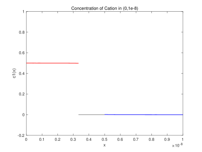
Figure 4: Profile of $c_{1}(x;\nu)$ over $[0,1]$. Note that $c_{10}(x)=0$ for $x\in(a,b)$ and, for $x\in(b,1)$, $c_{10}(x)=O(\sqrt{R})$ is not zero but small for $R=10^{-5}$ chosen for the numerics.

Figure 5: Profile of $\phi(x;\nu)$ over $[0,1]$

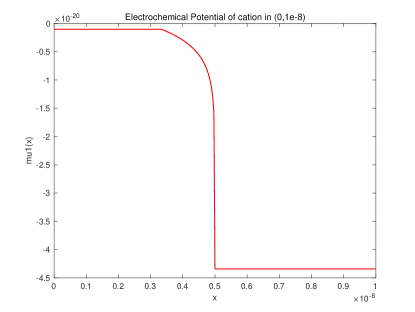
Figure 6: Profile of $\mu_{1}(x;\nu)$ over $[0,1]$. Note the large drop of $\mu_{1}$ over the interval $(a,b)=(1/3,1/2)$ and the nearly constant values over the other two subintervals.

5 Declining phenomenon and internal dynamics

In this section, we will show that large permanent charge is a mechanism for the declining phenomenon described in the introduction. Recall that, by the declining phenomenon, we mean the following observed experimentally.

For fixed $V$ and $L_{1}=L_{2}=L$, as $R_{1}=R_{2}=R$ decreases to zero, the flux of counterion ($J_{2}$ in the setting since $Q_{0}>0$) decreases monotonically to zero.

This phenomenon is rather counterintuitive since the transmembrane electrochemical potential for the counter-ion

$$\mu_{2}(0)-\mu_{2}(1)=z_{2}V+\ln L_{2}-\ln R_{2}\to+\infty\;\mbox{ as }\;R_{2}=R\to 0.$$

5.1 Experimental phenomena are consistent with our analysis

The result in (3.2) actually justifies the observation, up to the leading order $J_{20}$ in $\nu$ for $\nu$ near $0$ (or for $Q_{0}\to+\infty$); that is,

Proposition 5.1.

The leading order term $J_{20}$ of the flux is monotone and concave downward as a function of $R$ and, as $R\to 0$, $J_{20}\to 0$.

Proof.

Indeed, from the expression of $J_{20}$ in (3.2) and treating $J_{20}$ as a function of $w$ where $R=w^{2}$ for convenience, one has

$$J_{20}(w)=\frac{\sqrt{L}}{2H(1)}\frac{\sqrt{e^{-V}L}w-w^{2}}{(1-\beta)\sqrt{L}+\alpha\sqrt{e^{-V}}w}.$$

It is clear that $J_{20}(w)\to 0^{+}$ as $w\to 0^{+}$. Note that the derivative of $J_{20}$ in $w$ is

$$J_{20}^{\prime}(w)=\frac{1}{2H(1)}\frac{(1-\beta)L\sqrt{e^{-V}}-2(1-\beta)\sqrt{L}w-\alpha\sqrt{e^{-V}}w^{2}}{[(1-\beta)\sqrt{L}+\alpha\sqrt{e^{-V}}w]^{2}}.$$

Thus, from the expression of the numerator,

if $w$ is smaller than some $w_{0}$, then $J_{20}^{\prime}(w)>0$,

and hence, as $w\to 0^{+}$ (or equivalently, $R_{2}=R\to 0$) monotonically over the interval $[0,w_{0}]$, $J_{20}(w)\to 0$ monotonically.

It is not hard to show that for $R_{2}=R\geq 0$ but smaller than some positive value, the graph of $J_{20}$ as a function of $R$ is concave downward. ∎

In Figure 7, the horizontal axis is for $R$ and the vertical for $J_{20}$. We fix $V=0.425$ and $L=0.5$ as in (4.2), and vary $R\in(0,10^{-3}]$. The monotonicity and concave downward features of the graph are apparent.

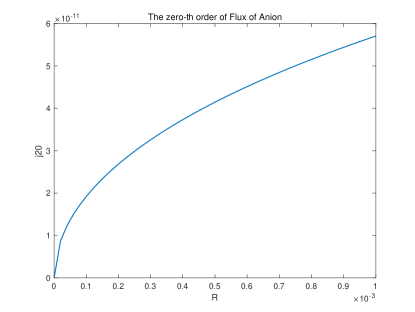
Figure 7: Declining curve: $J_{20}$ vs $R$ for $R\in(0,10^{-3}]$ with $L=0.5$ and $V=0.425$.

Remark 5.1.

We comment that, for large permanent charge, the declining curve phenomenon occurs when the transmembrane electrochemical potential $\mu_{2}(0)-\mu_{2}(1)$ is increasing to infinity in a particular way; that is, as $R\to 0$. If one increases the transmembrane electrochemical potential $\mu_{2}(0)-\mu_{2}(1)$ in a different manner, for example, as $|V|\to\infty$ or as $L\to\infty$, Corollary 3.2 shows that the declining curve phenomenon does not happen.

It is also important to note that, when the next order term $J_{21}\nu$ is considered, then, as $R_{2}=R\to 0$, $J_{21}\to\infty$. But, if $R\to 0$ and $\nu\ln R\to 0$, then $J_{21}\nu\to 0$. Thus, only when $\nu$ is very small ($Q_{0}$ is very large), is the term $J_{21}\nu$ not significant, and hence, the term $J_{20}$ dominates the described behavior. ∎

5.2 Mechanism of declining phenomena from the profiles

Recall, from the Nernst-Planck equation in (2.13) that

$$-J_{2}=\frac{1}{k_{B}T}D_{2}(x)h(x)c_{2}(x)\frac{d}{dx}\mu_{2}(x).$$

Since $D_{2}(x)$ and $h(x)$ are fixed, we will treat them as of order $O(1)$ quantities so that they do not contribute much to the near zero flux scenario as $R\to 0$. Thus, as far as the near zero flux mechanism is concerned, one has

$$-J_{2}\approx c_{2}(x)\frac{d}{dx}\mu_{2}(x).$$ (5.1)

One sees that the gradient of the electrochemical potential $\frac{d}{dx}\mu_{2}(x)$ is the main driving force for the flux $J_{2}$. Intuitively, large drop of (or transmembrane) electrochemical potential $\mu_{2}(0)-\mu_{2}(1)$ of $\mu_{2}$ produces large flux $J_{2}$. In this sense, the declining curve phenomenon is rather counterintuitive. A careful look at (5.1) reveals that there is only one possibility for the declining curve phenomenon; that is, whenever $\frac{d}{dx}\mu_{2}(x)$ is large, $c_{2}(x)$ has to be much smaller in order to produce a small flux $|J_{2}|$. We will apply the analytical results of the internal dynamics from ([45]) to show that this is indeed the case.

For our setup, there are three regions of permanent charge $Q(x)$: $Q(x)=0$ for $x\in[0,a)$ and $x\in(b,1]$ and $Q(x)=2Q_{0}$ for $x\in[a,b]$ with large $Q_{0}$ or small $\nu$ with ${\nu}=1/{Q_{0}}$.

For fixed $V$ and $L$, $\mu_{2}(0)-\mu_{2}(1)=z_{2}V+\ln L-\ln R\approx-\ln R\gg 1$ for small $R$. We need to understand

(i) HOW the electrochemical potential $\mu_{2}$ drops an order $O(-\ln R)\gg 1$ over the interval $x\in[0,1]$;

(ii) HOW $J_{2}$ can be small, for small $\nu$ and $R$, at every $x\in[0.1]$;

(iii) Most importantly, HOW the above two things, with the constraint (5.1), can happen simultaneously.

There are two small parameters $\nu$ and $R$ in our considerations. The relative sizes of these two parameters is relevant for the result. We will assume $\nu\ln R\ll 1$.

We now discuss what happens over each subinterval based on the approximated (of zeroth order in $\varepsilon$) functions of profiles. To do so, let

$$(\phi(x;\varepsilon,\nu),c_{k}(x;\varepsilon,\nu),J_{k}(\varepsilon,\nu))=(\phi(x;\nu),c_{k}(x;\nu),J_{k}(\nu))+O(\varepsilon)$$

be the solution of the boundary value problem. For $\nu>0$ small, one has the following expansions

$$J_{2}(\nu)=J_{20}+J_{21}\nu+O(\nu^{2}),$$

where $J_{20}$ and $J_{21}$ are given in (3.2). The expansions in $\nu$ for $\phi(x;\nu)$, $c_{1}(x;\nu)$, and $c_{2}(x;\nu)$ are not regular and are qualitatively different over the subintervals $(0,a)$, $(a,b)$ and $(b,1)$. They will be given explicitly in each subsection below for us to understand what happens over each subinterval.

5.2.1 Internal dynamics over the interval $(0,a)$

The leading order terms of $(\phi,c_{2})$ are derived in [45]. One has

Proposition 5.2.

For $x\in(0,a)$,

$$\phi(x;\nu)= \phi_{0}(x)+\phi_{1}(x)\nu+O(\nu^{2})\mbox{ with }$$

$$\phi_{0}(x)= V-\ln\Big{(}1-\frac{J_{20}}{2L}H(x)\Big{)},\quad\phi_{1}(x)=-\frac{c_{21}(x)}{c_{20}(x)}+\frac{2J_{11}}{J_{20}}\ln{\frac{c_{20}(x)}{L}};$$

$$c_{20}(x)= L-\frac{J_{20}}{2}H(x),\quad c_{21}(x)=-\frac{J_{11}+J_{21}}{2}H(x);$$

$$\mu_{20}(x)= -V+2\ln{c_{20}(x)}-\ln{L},\quad\mu_{21}(x)=2\left(\frac{c_{21}(x)}{c_{20}(x)}-\frac{J_{11}}{J_{20}}\ln{\frac{c_{20}(x)}{L}}\right).$$

Figure 8 shows profiles of $c_{2}(x;\nu)$, $\phi(x;\nu)$ and $\mu_{2}(x;\nu)$ over the interval $(0,a)$.

Corollary 5.3.

Over the interval $(0,a)$, $c_{2}(x;\nu)=O(1)$ BUT

$$\mu_{2}^{\prime}(x;\nu)=-\frac{J_{20}}{h(x)c_{20}(x)}+O(\nu\ln R)=O(\sqrt{R},\nu\ln R).$$

Therefore, from (5.1),

$$J_{2}\approx c_{2}(x)\frac{d}{dx}\mu_{2}(x;\nu)=O(1)O(\sqrt{R},\nu\ln R)=O(\sqrt{R},\nu\ln R)$$

and $\mu_{2}(x)$ drops an order of $O(\sqrt{R},\nu\ln R)$ over the interval $(0,a)$.

In particular, for zeroth order in $\nu$, $J_{2}\approx J_{20}=O(\sqrt{R})$ and $\mu_{2}^{\prime}(x)=O(\sqrt{R})$ over the interval $(0,a)$.

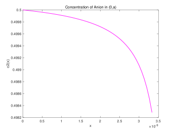
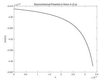
Figure 8: Profiles of $c_{k}(x;\nu)$, $\phi(x;\nu)$, and $\mu_{k}(x;\nu)$ over interval $[0,a]$.

5.2.2 Internal dynamics over the interval $(a,b)$

It follows from [45] that

Proposition 5.4.

For $x\in(a,b)$,

$$\phi(x;\nu)= -\ln\nu+\phi_{0}(x)+\phi_{1}(x)\nu+O(\nu^{2})\;\mbox{ with }$$

$$\phi_{0}(x)= \ln{R}-2\ln{B_{0}}+\ln{2},$$

$$\phi_{1}(x)= \phi_{1}^{a}-A_{0}+\frac{J_{20}}{2}(H(x)-H(a));$$

$$c_{2}(x;\nu)= \frac{1}{\nu}+\left(\frac{1}{2}A_{0}^{2}-J_{11}(H(x)-H(a))\right)\nu+O(\nu^{2});$$

$$\mu_{20}(x)= -\ln{R}+2\ln{B_{0}}-\ln{2},$$

$$\mu_{21}(x)= -\phi_{1}^{a}+A_{0}-\frac{J_{20}}{2}(H(x)-H(a)),$$

$$\mu_{22}(x)= \frac{1}{2}A_{0}^{2}-J_{11}(H(x)-H(a));$$

where

$$A_{0}= \frac{\sqrt{e^{V}L}((1-\beta)L+\alpha R)}{(1-\beta)\sqrt{e^{V}L}+\alpha\sqrt{R}},\quad B_{0}=\frac{\sqrt{R}((1-\beta)L+\alpha R)}{(1-\beta)\sqrt{e^{V}L}+\alpha\sqrt{R}},$$

$$A_{1}= \frac{2(\beta-\alpha)^{2}(L-A_{0})^{2}-\alpha^{2}(A_{0}^{2}-B_{0}^{2})\ln{\frac{B_{0}L}{A_{0}R}}}{4(\beta-\alpha)((1-\beta)L+\alpha R)(L-A_{0})}A_{0}B_{0},$$

$$B_{1}= -\frac{(1-\beta)\left(2(\beta-\alpha)^{2}(L-A_{0})^{2}-\alpha^{2}(A_{0}^{2}-B_{0}^{2})\ln{\frac{B_{0}L}{A_{0}R}}\right)}{4\alpha(\beta-\alpha)((1-\beta)L+\alpha R)(L-A_{0})}A_{0}B_{0},$$

$$\phi_{1}^{a}= \frac{\ln{\frac{B_{0}}{R}}}{\ln{\frac{B_{0}L}{A_{0}R}}}\left(2\Big{(}\frac{B_{1}}{B_{0}}-\frac{A_{1}}{A_{0}}\Big{)}+\frac{\beta-\alpha}{\alpha}(L-A_{0})\right)-2\frac{B_{1}}{B_{0}}-\frac{\beta}{\alpha}(L-A_{0})+L.$$

The profiles of $c_{2}(x;\nu)$, $\phi(x;\nu)$, and $\mu_{2}(x;\nu)$ are shown in Figure 9.

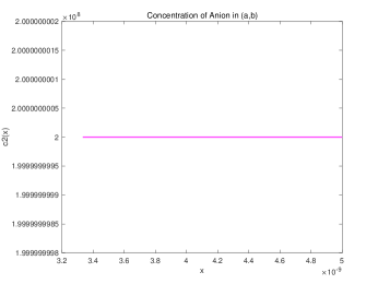
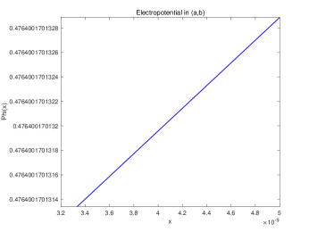
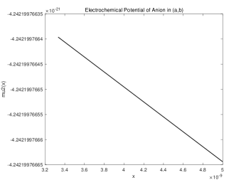
Figure 9: Profiles of $c_{2}(x;\nu)$, $\phi(x;\nu)$, and $\mu_{2}(x;\nu)$ over interval $[a,b]$

Note that, over this interval, $c_{2}(x;\nu)$ is singular in $\nu$. To understand what happens to the internal dynamics for anions over the interval $(a,b)$, we need to resolve this singularity by considering at least $O(\nu)$-terms.

Corollary 5.5.

Over the interval $(a,b)$, $c_{2}(x;\nu)=O(1/\nu)\gg 1$ and $\;\mu_{2}(x;\nu)=O(\ln R)\gg 1$ BUT

$$\mu_{2}^{\prime}(x;\nu)\approx\mu_{21}^{\prime}(x)\nu=-\frac{J_{20}}{2h(x)}\nu=O(\nu\sqrt{R}).$$

Therefore, from (5.1),

$$J_{2}\approx O(1/\nu)O(\nu\sqrt{R})=O(\sqrt{R})\;\mbox{ and }\;\mu_{2}(x;\nu)\;\mbox{ only drops }\;O(\nu\sqrt{R})\;\mbox{ over }\;(a,b).$$

Remark 5.2.

Note that $\mu_{2}(x)$ drops much less over the interval $(a,b)$ than its drop over the interval $(0,a)$. But both drops are small and contribute nearly nothing to the total drop $\mu_{2}(0)-\mu_{2}(1)=O(-\ln R)\gg 1$. The only way to realize the large total drop $\mu_{2}(0)-\mu_{2}(1)$ is that $\mu_{2}(x)$ drops A LOT over the subinterval $(b,1)$. Indeed, this is the case as claimed below. ∎

5.2.3 Internal dynamics over the interval $(b,1)$

Proposition 5.6.

For $x\in(b,1)$,

$$\phi(x;\nu)= \phi_{0}(x)+\phi_{1}(x)\nu+O(\nu^{2})\;\mbox{ with }$$

$$\phi_{0}(x)= \ln R-\ln c_{20}(x),$$

$$\phi_{1}(x)= \phi_{1}^{b}-\frac{1}{2}\left(B_{0}^{2}-\frac{2B_{1}-B_{0}^{2}}{B_{0}}\right)-\frac{B_{0}c_{21}(x)-B_{1}c_{20}(x)}{B_{0}c_{20}(x)}+\frac{2J_{11}}{J_{20}}\ln{\frac{c_{20}(x)}{B_{0}}};$$

$$c_{20}(x)= B_{0}-\frac{J_{20}}{2}(H(x)-H(b)),\quad c_{21}(x)=B_{1}-\frac{J_{11}+J_{21}}{2}(H(x)-H(b));$$

$$\mu_{20}(x)= 2\ln{c_{20}(x)}-\ln R,\quad\mu_{21}(x)=\frac{c_{21}(x)}{c_{20}(x)}-\phi_{1}(x);$$

where

$$\phi_{1}^{b}= \frac{\ln{\frac{B_{0}}{R}}}{\ln{\frac{B_{0}L}{A_{0}R}}}\left(2\Big{(}\frac{B_{1}}{B_{0}}-\frac{A_{1}}{A_{0}}\Big{)}+\frac{\beta-\alpha}{\alpha}(L-A_{0})\right)-2\frac{B_{1}}{B_{0}}+B_{0}.$$

The profiles of $c_{2}(x;\nu)$, $\phi(x;\nu)$, and $\mu_{2}(x;\nu)$ over $(b,1)$ are shown in Figure 10.

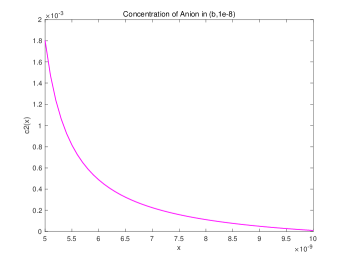
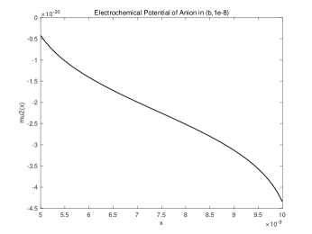
Figure 10: Profiles of $c_{2}(x;\nu)$, $\phi(x;\nu)$, and $\mu_{2}(x;\nu)$ over interval $[b,1]$

Corollary 5.7.

Over the interval $(b,1)$, noting $B_{0}=O(\sqrt{R})$, $c_{20}(x)$ changes from $c_{20}(b)=B_{0}=O(\sqrt{R})$ to $c_{20}(1)=R$ monotonically, and $\mu_{2}(x)$ changes from $\mu_{2}(b)=O(1)$ to $\mu_{2}(1)=\ln R$.

Therefore, for $x\in(b,1)$, from (5.1),

$$J_{2}\approx O(\sqrt{R})\;\mbox{ and }\;\mu_{2}(x)\;\mbox{ drops }\;O(-\ln R)\;\mbox{ over }\;(b,1).$$

Remark 5.3.

Note that, over this interval, the order of $\mu^{\prime}_{2}(x)$ varies in $x$ from $\mu^{\prime}_{2}(b)=O(1)$ to $\mu^{\prime}_{2}(1)=O(1/{\sqrt{R}})$ but overall drops is $O(-\ln R)$. This is different from what happened over the intervals $(0,a)$ and $(a,b)$. ∎

5.3 Summary of mechanism for declining phenomenon.

In summary, with the technical assumption that $\nu\ln R\leq\sqrt{R}$, we have, as $R\to 0$, $J_{2}=O(\sqrt{R})$ over the whole interval $(0,1)$ but with completely DIFFERENT scenarios over different subintervals $(0,a)$, $(a,b)$ and $(b,1)$. More precisely,

• over the subinterval $(0,a)$, one has $c_{2}(x)=O(1)$ but $\mu_{2}^{\prime}(x)=O(\sqrt{R})\ll 1$ so that $J_{2}=O(\sqrt{R})$; (Note that the drop of $\mu_{2}$ over the interval $(0,a)$ is of order $O(\sqrt{R})$, which has nearly no contribution to the drop of $\mu_{2}$ over the whole interval $(0,1)$.)

• over the subinterval $(a,b)$, $c_{2}(x)=O(1/{\nu})$ but $\mu_{2}^{\prime}(x)=O(\nu\sqrt{R})\ll 1$ so that $J_{2}=O(\sqrt{R})$; (Note that the drop of $\mu_{2}$ over the interval $(a,b)$ is of order $O(\nu\sqrt{R})$, which is even smaller than that over the subinterval $(0,a)$ and, of course, has nearly no contribution to the drop of $\mu_{2}$ over the whole interval $(0,1)$.)

• over the subinterval $(b,1)$, different from what happened over each of the previous two subintervals, the orders of $c_{2}(x)$ and $\mu_{2}^{\prime}(x)$ are NOT uniform in $x\in(b,1)$ but the drop of $\mu_{2}(x)$ of $O(\ln R)$ is fully realized over this subinterval (see Remark 5.3).

Here we provide the profiles of concentration (Fig. 11), electric field (Fig. 12) and electrochemical potential (Fig. 13) of the anion over the whole interval $[0,1]$. The figures of $c_{k}(x)$ and $\phi(x)$ over interval $(0,x_{0})$ are not continue, because we make the plots of system (LABEL:ssPNP) with $\varepsilon=0$. For the limiting system at $x=a$ and $x=b$, there are two fast layers, $c_{k}(x)$ and $\phi(x)$ changes very fast, but $\mu_{k}(x)$ keeps the same value in fast layers. Recall that $\mu_{2}^{\delta}=\mu_{2}(0)-\mu_{2}(1)=k_{B}T(-V+\ln{L}-\ln{R})$, if $R=10^{-5}$, then $\mu_{2}^{\delta}\sim 2.4780\times 10^{-31}$, that’s why in the last figure, $\mu_{2}(x)$ can not reach the infinity.

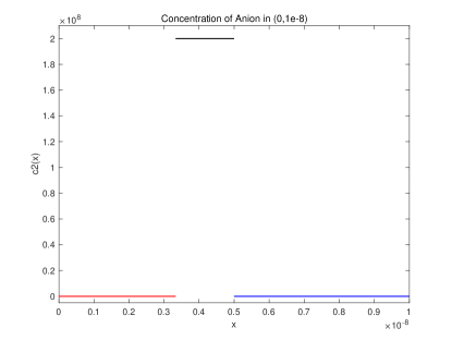
Figure 11: Profile $c_{2}(x;\nu)$ over $[0,1]$

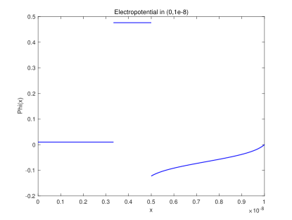
Figure 12: Profile of $\phi(x;\nu)$ over $[0,1]$

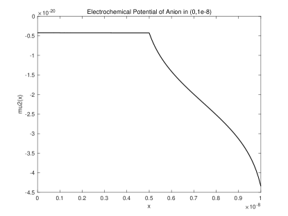
Figure 13: Profile of $\mu_{2}(x;\nu)$ over $[0,1]$

6 Concluding remarks

In this work, we examine effects of large permanent charges on ionic flow through ion channels based on a quasi-one dimensional Poisson-Nernst-Planck model. We show that one of the defining properties of transporters, obligatory exchange, can arise in an open channel with just one structure. When the permanent charge is large, the current carried by counter ions, majority charge carriers with the opposite sign as the permanent charge, can decline, even to zero, as the driving force (the gradient of electrochemical potential) increases. We also show that large permanent charges essentially inhibit the flux of co-ions, regardless of the magnitude of transmembrane electrochemical potential.

Acknowledgements. It is a pleasure to thank Mordy Blaustein, Don Hilgemann and Ernie Wright for help with the literature of transporters and Chris Miller for help with the original formulation of the declining phenomenon in Section 5. LZ thanks the University of Kansas for its hospitality during her visit from Oct. 2016-Oct. 2017 when this research is conducted. LZ is partially supported by NNSF of China grants no. 11431008 and no. 11771282, and the Joint Ph.D. Training Program sponsored by the Chinese Scholarship Council.

References

- [1] J. N. Abelson, M. I. Simon, S. V. Ambudkar, and M. M. Gottesman, ABC Transporters: Biochemical, Cellular, and Molecular Aspects. Academic Press, 1998.
- [2] P. F. Baker, M. P. Blaustein, A. L. Hodgkin, and R. A. Steinhardt, The influence of calcium on sodium efflux in squid axons. J. Physiol. 200 (1969), 431-458.
- [3] M. P. Blaustein and W. J. Lederer, Sodium/Calcium Exchange: Its Physiological Implications. Physiol. Rev. 79 (1999), 763-854.
- [4] P. Chlanda, E. Mekhedov, H. Waters, C. L. Schwartz, E. R. Fischer, R. J. Ryham, F. S. Cohen, P. S. Blank, and J. Zimmerberg, The hemifusion structure induced by influenza virus haemagglutinin is determined by physical properties of the target membranes. Nat. Microbiol. 1 (2016), 16050.
- [5] B. Eisenberg and W. Liu, Relative dielectric constants and selectivity ratios in open ionic channels. Mol. Based Math. Biol. 5 (2017), 125-137.
- [6] B. Eisenberg, Shouldn’t we make biochemistry an exact science? ASBMB Today 13 (2014), 36-38.
- [7] B. Eisenberg, Ions in Fluctuating Channels: Transistors Alive. Fluctuation and Noise Letters 11 (2012), 1240001.
- [8] B. Eisenberg, Crowded Charges in Ion Channels. Advances in Chemical Physics 148 (ed. Stuart A. Rice and Aaron R. Dinner), 77-223. John Wiley & Sons, Inc., 2012.
- [9] R. S. Eisenberg, Computing the field in proteins and channels. J. Memb. Biol. 150 (1996), 1-25.
- [10] R. S. Eisenberg. Atomic Biology, Electrostatics and Ionic Channels. In New Developments and Theoretical Studies of Proteins (ed. R. Elber), 269-357. World Scientific: Philadelphia, 1996.
- [11] R. S. Eisenberg. Channels as enzymes: Oxymoron and Taytology. J. Memb. Biol. 115 (1990), 1-12.
- [12] B. Eisenberg and W. Liu, Poisson-Nernst-Planck systems for ion channels with permanent charges. SIAM J. Math. Anal. 38 (2007), 1932-1966.
- [13] B. Eisenberg, W. Liu, and H. Xu, Reversal permanent charge and reversal potential: case studies via classical Poisson-Nernst-Planck models. Nonlinearity 28 (2015), 103-128.
- [14] O. Frohlich and R. B. Gunn, Erythrocyte anion transport: the kinetics of a single-site obligatory exchange system. Biochem. Biophys. Acta 864 (1986), 169-194.
- [15] D. Gillespie, A singular perturbation analysis of the Poisson-Nernst-Planck system: Applications to Ionic Channels. Ph.D. Dissertation, Rush University at Chicago, 1999.
- [16] J. Griffiths and C. Sansom, The Transporter Facts Book. Academic Press, 1997.
- [17] F. Helfferich, Ion Exchange (1995 Reprint). McGraw Hill reprinted by Dover, 1962.
- [18] B. Hille, Ion Channels of Excitable Membranes. (3rd ed.) Sinauer Associates Inc., 2001.
- [19] B. Hille, Transport Across Cell Membranes: Carrier Mechanisms, Ch. 2 in Textbook of Physiology Vol. 1 (eds H.D. Patton et al.), 24-47. Saunders, 1989.
- [20] A. L. Hodgkin, The ionic basis of electrical activity in nerve and muscle. Biol. Rev. 26 (1951), 339-409.
- [21] S. Ji, B. Eisenberg, and W. Liu, Flux Ratios and Channel Structures. J. Dyn. Diff. Equat. (2017). https://doi.org/10.1007/s10884-017-9607-1.
- [22] S. Ji and W. Liu, Poisson-Nernst-Planck systems for ion flow with Density Functional Theory for hard-sphere potential: I-V relations and critical potentials. Part I: Analysis. J. Dyn. Diff. Equat. 24 (2012), 955-983.
- [23] S. Ji, W. Liu, and M. Zhang, Effects of (small) permanent charge and channel geometry on ionic flows via classical Poisson-Nernst-Planck models, SIAM J. Appl. Math. 75 (2015), 114-135.
- [24] R. D. Keynes and R. C. Swan, The effect of external sodium concentration on the sodium fluxes in frog skeletal muscle. J. Physiol. 147 (1959), 591-625.
- [25] G. Lin, W. Liu, Y. Yi, and M. Zhang, Poisson-Nernst-Planck systems for ion flow with a local hard-sphere potential for ion size effects. SIAM J. Appl. Dyn. Syst. 12 (2013), 1613-1648.
- [26] W. Liu. Geometric singular perturbation approach to steady-state Poisson-Nernst-Planck systems. SIAM J. Appl. Math. 65 (2005), 754-766.
- [27] W. Liu, One-dimensional steady-state Poisson-Nernst-Planck systems for ion channels with multiple ion species. J. Differential Equations 246 (2009), 428-451.
- [28] W. Liu and B. Wang, Poisson-Nernst-Planck systems for narrow tubular-like membrane channels. J. Dyn. Diff. Equat. 22 (2010), 413-437.
- [29] W. Liu, X. Tu, and M. Zhang, Poisson-Nernst-Planck systems for ion flow with Density Functional Theory for hard-sphere potential: I-V relations and critical potentials. Part II: Numerics. J. Dyn. Diff. Equat. 24 (2012), 985-1004.
- [30] W. Liu and H. Xu, A complete analysis of a classical Poisson-Nernst-Planck model for ionic flow. J. Differential Equations 258 (2015), 1192-1228.
- [31] M. Lu, J. Symersky, M. Radchenko, A. Koide, Y. Guo, R. Nie, and S. Koide, Structures of a Na+-coupled, substrate-bound MATE multidrug transporter. Proceedings of the National Academy of Sciences 110 (2013), 2099-2104.
- [32] H. Miedema, M. Vrouenraets, J. Wierenga, W. Meijberg, G. Robillard, and B. Eisenberg, A Biological Porin Engineered into a Molecular, Nanofluidic Diode. Nano Lett. 7 (2007), 2886-2891.
- [33] W. Nonner and R. S. Eisenberg, Ion permeation and glutamate residues linked by Poisson-Nernst-Planck theory in L-type Calcium channels. Biophys. J. 75 (1998), 1287-1305.
- [34] R. F. Pierret, Semiconductor Device Fundamentals. Addison Wesley, 1996.
- [35] B. Sakmann and E. Neher, Single Channel Recording. (2nd ed.), Plenum, 1995.
- [36] W. D. Stein and T. Litman, Channels, carriers, and pumps: an introduction to membrane transport. Elsevier, 2014.
- [37] R. B. Stockbridge, L. Kolmakova-Partensky, T. Shane, A. Koide, A. Koide, C. Miller, and S. Newstead, Crystal structures of a double-barrelled fluoride ion channel. Nature 525 (2015), 548-551.
- [38] S. M. Sze, Physics of Semiconductor Devices. John Wiley & Sons, 1981.
- [39] F. L. Theodoulou and I. D. Kerr, ABC transporter research: going strong 40 years on. Biochemical Society Transactions 43 (2015), 1033-1040.
- [40] D. Tosteson, Membrane Transport: People and Ideas. American Physiological Society, 1989.
- [41] H. H. Ussing, The distinction by means of tracers between active transport and diffusion. Acta physiologica Scandinavica 19 (1949), 43-56.
- [42] H. H. Ussing, Interpretation of the exchange of radio-sodium in isolated muscle. Nature 160 (1947), 262-263.
- [43] D. Vasileska, S. M. Goodnick, and G. Klimeck, Computational Electronics: Semiclassical and Quantum Device Modeling and Simulation. Vol. 764, CRC Press, 2010.
- [44] W. Wang and R. MacKinnon, Cryo-EM Structure of the Open Human Ether-a-go-go-Related K+ Channel hERG. Cell 169 (2017), 422-430 e410.
- [45] L. Zhang and W. Liu, Poisson-Nernst-Planck systems for ion channels with large permanent charges. Preprint.
- [46] J. Zheng and M. C. Trudeau, Handbook of ion channels. CRC Press, 2015.