Higher Order Convergent Fast Nonlinear Fourier Transform

Abstract

It is demonstrated is this letter that linear multistep methods for integrating ordinary differential equations can be used to develop a family of fast forward scattering algorithms with higher orders of convergence. Excluding the cost of computing the discrete eigenvalues, the nonlinear Fourier transform (NFT) algorithm thus obtained has a complexity of $\mathop{O}(KN+C_{p}N\log^{2}N)$ such that the error vanishes as $\mathop{O}(N^{-p})$ where $p\in\{1,2,3,4\}$ and $K$ is the number of eigenvalues. Such an algorithm can be potentially useful for the recently proposed NFT based modulation methodology for optical fiber communication. The exposition considers the particular case of the backward differentiation formula ($C_{p}=p^{3}$) and the implicit Adams method ($C_{p}=(p-1)^{3}$) of which the latter proves to be the most accurate family of methods for fast NFT.

I Introduction

This paper deals with the algorithmic aspects of the nonlinear Fourier transform (NFT) based modulation scheme which aims at exploiting the nonlinear Fourier spectrum (NF) for optical fiber communication [1]. These novel modulation [2, 3] techniques can be viewed as an extension of the original ideas of Hasegawa and Nyu who proposed what they coined as eigenvalue communication in the early 1990s [4]. One of the key ingredients in various NFT-based modulation techniques is the fast forward NFT which can be used to decode information encoded in the discrete and/or the continuous part of the nonlinear Fourier spectrum. A thorough description of the discrete framework (based on one-step methods) for various fast forward/inverse NFT algorithms was presented in [5] where it was shown that one can achieve a complexity of $\mathop{O}(N\log^{2}N)$ in computing the scattering coefficients in the discrete form. If the eigenvalues are known beforehand, then the NFT has an overall complexity of $\mathop{O}(KN+N\log^{2}N)$ such that the error vanishes as $\mathop{O}(N^{-2})$ where $N$ is the number of samples of the signal and $K$ is the number of eigenvalues. Interestingly enough, the complexity of the fast inverse NFT proposed in [6, 7] also turns out to be $\mathop{O}(KN+N\log^{2}N)$ with error vanishing as $\mathop{O}(N^{-2})$.

In this letter, we present new fast forward scattering algorithms where the complexity of computing the discrete scattering coefficients is $\mathop{O}(C_{p}N\log^{2}N)$. If the eigenvalues are known beforehand, the NFT of a given signal can be computed with a complexity of $\mathop{O}(KN+C_{p}N\log^{2}N)$ such that the error vanishes as $\mathop{O}(N^{-p})$ where ($p\in\{1,2,3,4\}$) and $K$ is the number of eigenvalues. In particular, we demonstrate in this work that using $m$-step ($m\in\{1,2,3,4\}$) backward differentiation formula (BDF) and $m$-step ($m\in\{1,2,3\}$) implicit Adams (IA) method [8] one can obtain fast forward NFT algorithms with order of convergence given by $p=m$ and $p=m+1$, respectively.

The starting point of our discussion is the Zakharov and Shabat (ZS) [9] scattering problem which can be stated as: For $\zeta\in\mathbb{R}$ and $\mathbf{v}=(v_{1},v_{2})^{\intercal}$,

$$\mathbf{v}_{t}=-i\zeta\sigma_{3}\mathbf{v}+U(t,x)\mathbf{v},$$ (1)

where $\sigma_{3}=\text{diag}(1,-1)$ and the potential $U(t,x)$ is defined by $U_{11}=U_{22}=0,\,U_{12}=q(t,x)$ and $U_{21}=r(t,x)$ with $r=\kappa q^{*}$ ($\kappa\in\{+1,-1\}$). The parameter $\zeta\in\mathbb{R}$ is known as the spectral parameter and $q(t,x)$ is the complex-valued function associated with the slow varying envelop of the optical field which evolves along the fiber according to the nonlinear Schrödinger equation (NSE), stated in its normalized form,

$$iq_{x}=q_{tt}-2\kappa|q|^{2}q.$$ (2)

The NSE provides a satisfactory description of pulse propagation in an optical fiber in the path-averaged formulation [10] under low-noise conditions where $t$ is the retarded time and $x$ is the distance along the fiber. In the following, the dependence on $x$ is suppressed for the sake of brevity. Here, $q(t)$ is identified as the scattering potential. The solution of the ZS scattering problem (1) consists in finding the so called scattering coefficients which are defined through special solutions of (1) known as the Jost solutions. The Jost solutions of the first kind, denoted by $\bm{\psi}(t;\zeta)$, has the asymptotic behavior $\bm{\psi}(t;\zeta)e^{-i\zeta t}\rightarrow(0,1)^{\intercal}$ as $t\rightarrow\infty$. The Jost solutions of the second kind, denoted by $\bm{\phi}(t,\zeta)$, has the asymptotic behavior $\bm{\phi}(t;\zeta)e^{i\zeta t}\rightarrow(1,0)^{\intercal}$ as $t\rightarrow-\infty$.

For the focusing NSE (i.e., $\kappa=-1$ in (2)), the nonlinear Fourier spectrum for the potential $q(t)$ comprises a discrete and a continuous spectrum. The discrete spectrum consists of the so-called eigenvalues $\zeta_{k}\in\mathbb{C}_{+}$, such that $a(\zeta_{k})=0$, and, the norming constants $b_{k}$ such that $\bm{\phi}(t;\zeta_{k})=b_{k}\bm{\psi}(t;\zeta_{k})$. Note that $(\zeta_{k},\,b_{k})$ describes a bound state or a solitonic state associated with the potential. For convenience, let the discrete spectrum be denoted by the set

$$\mathfrak{S}_{K}=\{(\zeta_{k},\,b_{k})\in\mathbb{C}^{2}|\,\operatorname{Im}{\zeta_{k}}>0,\,k=1,2,\ldots,K\}.$$ (3)

Note that for the defocussing NSE (i.e., $\kappa=+1$ in (2)), the discrete spectrum is empty. The continuous spectrum, also referred to as the reflection coefficient, is defined by $\rho(\xi)={b(\xi)}/{a(\xi)}$ for $\xi\in\mathbb{R}$.

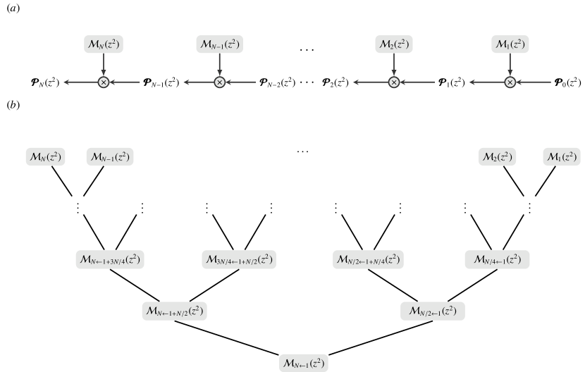
Figure 1: The figure shows the sequential approach to forward scattering in $(a)$. A more efficient approach is the divide-and-conquer strategy shown in $(b)$ where the transfer matrices $\{\mathcal{M}_{n}(z^{2})\}$ are multiplied pairwise culminating in the full transfer matrix $\mathcal{M}_{N\leftarrow 1}(z^{2})$. All polynomial products are formed using the FFT algorithm. Here $\mathcal{M}_{n\leftarrow m}(z^{2})$ denotes the cumulative transfer matrix $\mathcal{M}_{n}(z^{2})\times\ldots\times\mathcal{M}_{m+1}(z^{2})\times\mathcal{M}_{m}(z^{2})$.

The letter first discusses the numerical discretization based on linear multistep methods, BDF and IA, along with the algorithmic aspects. This is followed by numerical experiments that verify the expected behavior of the algorithms.

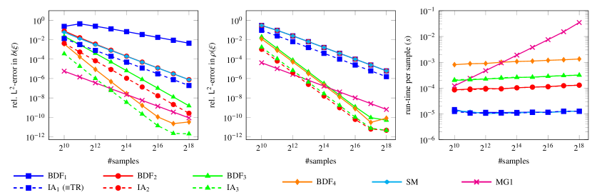
Figure 2: The figure shows a comparison of convergence behavior and run-time of NFT algorithms based on the discretization schemes, namely, BDF_m ($m\in\{1,2,3,4\}$), IA_m ($m\in\{1,2,3\}$), SM and MG1 (see Sec. III). The method IA₁ is identical to the trapezoidal rule (TR).

The letter first discusses the numerical discretization based on linear multistep methods, BDF and IA, along with the algorithmic aspects. This is followed by numerical experiments that verify the expected behavior of the algorithms.

II The Numerical Scheme

In order to develop the numerical scheme, we begin with the transformation $\tilde{\mathbf{v}}=e^{i\sigma_{3}\zeta t}\mathbf{v}$ so that (1) becomes

$$\tilde{\mathbf{v}}_{t}=\widetilde{U}\tilde{\mathbf{v}},\quad\widetilde{U}=e^{i\sigma_{3}\zeta t}Ue^{-i\sigma_{3}\zeta t}=\begin{pmatrix}0&qe^{2i\zeta t}\\ re^{-2i\zeta t}&0\end{pmatrix}.$$ (4)

In order to discuss the discretization scheme, we take an equispaced grid defined by $t_{n}=T_{1}+nh,\,\,n=0,1,\ldots,N,$ with $t_{N}=T_{2}$ where $h$ is the grid spacing. Define $\ell_{-},\ell_{+}\in\mathbb{R}$ such that $h\ell_{-}=-T_{1}$, $h\ell_{+}=T_{2}$. Further, let us define $z=e^{i\zeta h}$. For the potential functions sampled on the grid, we set $q_{n}=q(t_{n})$, $r_{n}=r(t_{n})$, $U_{n}=U(t_{n})$ and $\widetilde{U}_{n}=\widetilde{U}(t_{n})$. Discretization using the $m$-step BDF scheme ($m\in\{1,2,3,4\}$) reads as

$$\sum_{s=0}^{m}\alpha_{s}\widetilde{\mathbf{v}}_{n+s}=h\beta\widetilde{U}_{n+m}\tilde{\mathbf{v}}_{n+m}$$ (5)

where $\bm{\alpha}=(\alpha_{0},\alpha_{1},\ldots,\alpha_{m})$ and $\beta$ are known constants [8, Chap. III.1]. Discretization using the $m$-step IA method ($m\in\{1,2,3\}$) reads as

$$\tilde{\mathbf{v}}_{n+m}-\tilde{\mathbf{v}}_{n+m-1}=h\sum_{s=0}^{m}\beta_{s}\widetilde{U}_{n+s}\tilde{\mathbf{v}}_{n+s}$$ (6)

where $\bm{\beta}=(\beta_{0},\beta_{1},\ldots,\beta_{m})$ are known constants [8, Chap. III.1]. Both of these methods lead to a transfer matrix $\mathcal{M}_{n+m}(z^{2})\in\mathbb{C}^{2m\times 2m}$ of the form

$${\mathcal{M}}_{n+m}(z^{2})=\\ \begin{pmatrix}\gamma_{m-1}M^{(1)}_{n+m}&\gamma_{m-2}M^{(2)}_{n+m}&\ldots&\gamma_{1}M^{(m-1)}_{n+m}&\gamma_{0}M^{(m)}_{n+m}\\ \sigma_{0}&0&\ldots&0&0\\ 0&\sigma_{0}&\ldots&0&0\\ \vdots&\vdots&\ddots&\vdots&\vdots\\ 0&0&\ldots&\sigma_{0}&0\end{pmatrix},$$ (7)

where $\sigma_{0}=\operatorname{diag}(1,1)$ and $M^{(s)}_{n+m}=M^{(s)}_{n+m}(z^{2})\in\mathbb{C}^{2\times 2}$ so that

$$\boldsymbol{\mathcal{W}}_{n+m}={\mathcal{M}}_{n+m}(z^{2})\boldsymbol{\mathcal{W}}_{n+m-1}$$ (8)

where $\mathbf{w}_{n}=z^{n}\mathbf{v}_{n}$ and $\boldsymbol{\mathcal{W}}_{n}=(\mathbf{w}_{n},\mathbf{w}_{n-1},\ldots,\mathbf{w}_{n-m+1})^{\intercal}\in\mathbb{C}^{2m}$. For BDF schemes, we may set $\alpha_{m}\equiv 1$. Further, setting $Q_{n}=(h\beta)q_{n}$, $R_{n}=(h\beta)r_{n}$ and $\Theta_{n}=1-Q_{n}R_{n}$, we have $\gamma_{s}=-\alpha_{s}$ together with

$$M^{(s)}_{n+m}(z^{2})=\frac{1}{\Theta_{n+m}}\begin{pmatrix}1&z^{2s}Q_{n+m}\\ R_{n+m}&z^{2s}\end{pmatrix}.$$ (9)

For the IA methods, we have

$$M^{(1)}_{n+m}(z^{2})=\Theta^{-1}_{n+m}\times\\ \begin{pmatrix}1+z^{2}\bar{\beta}_{m-1}R_{n+m-1}Q_{n+m}&z^{2}Q_{n+m}+\bar{\beta}_{m-1}Q_{n+m-1}\\ R_{n+m}+z^{2}\bar{\beta}_{m-1}R_{n+m-1}&z^{2}+\bar{\beta}_{m-1}R_{n+m}Q_{n+m-1}\end{pmatrix},$$ (10)

where $Q_{n}=(h\beta_{m})q_{n}$, $R_{n}=(h\beta_{m})r_{n}$, $\Theta_{n}=1-Q_{n}R_{n}$. Also,

$$M^{(m-s)}_{n+m}(z^{2})=\frac{1}{\Theta_{n+m}}\begin{pmatrix}z^{2(m-s)}R_{n+s}Q_{n+m}&Q_{n+s}\\ z^{2(m-s)}R_{n+s}&R_{n+m}Q_{n+s}\end{pmatrix},$$ (11)

with $\gamma_{m-1}=1$ and $\gamma_{s}=\overline{\beta}_{s}$ for $s=0,1,\ldots,m-2$ where

$$\overline{\bm{\beta}}=\bm{\beta}/\beta_{m}=(\overline{\beta}_{0},\overline{\beta}_{1},\ldots,1).$$ (12)

Let us consider the Jost solution $\bm{\phi}(t;\zeta)$. We assume that $q_{n}=0$ for $n=-m+1,-m+2,\ldots,0$ so that $\bm{\phi}_{n}=z^{\ell_{-}}z^{-n}(1,0)^{\intercal}$ for $n=-m+1,-m+2,\ldots,0$. In order to express the discrete approximation to the Jost solutions, let us define the vector-valued polynomial

$$\mathbf{P}_{n}(z^{2})=\begin{pmatrix}P^{(n)}_{1}(z^{2})\\ P^{(n)}_{2}(z^{2})\end{pmatrix}\\ =\sum_{j=0}^{n}\mathbf{P}^{(n)}_{j}z^{2j}=\sum_{j=0}^{n}\begin{pmatrix}P^{(n)}_{1,j}\\ P^{(n)}_{2,j}\end{pmatrix}^{\intercal}z^{2j},$$ (13)

such that $\bm{\phi}_{n}=z^{\ell_{-}}z^{-n}\mathbf{P}_{n}(z^{2})$. The initial condition works out to be

$$\boldsymbol{\mathcal{W}}_{0}=z^{\ell_{-}}\begin{pmatrix}\bm{\phi}_{0}\\ z\bm{\phi}_{-1}\\ \vdots\\ z^{-m+1}\bm{\phi}_{-m+1}\end{pmatrix}=z^{\ell_{-}}\begin{pmatrix}\bm{P}_{0}(z^{2})\\ \bm{P}_{-1}(z^{2})\\ \vdots\\ \bm{P}_{-m+1}(z^{2})\end{pmatrix}\in\mathbb{C}^{2m},$$ (14)

yielding the recurrence relation

$$\boldsymbol{\mathcal{P}}_{n+m}(z^{2})={\mathcal{M}}_{n+m}(z^{2})\boldsymbol{\mathcal{P}}_{n+m-1}(z^{2}),$$ (15)

where $\boldsymbol{\mathcal{P}}_{n}(z^{2})=(\mathbf{P}_{n}(z^{2}),\mathbf{P}_{n-1}(z^{2}),\ldots,\mathbf{P}_{n-m+1}(z^{2}))^{\intercal}\in\mathbb{C}^{2m}$. The discrete approximation to the scattering coefficients is obtained from the scattered field: $\bm{\phi}_{N}=(a_{N}z^{-\ell_{+}},b_{N}z^{\ell_{+}})^{\intercal}$ yields $a_{N}(z^{2})={P}^{(N)}_{1}(z^{2})$ and $b_{N}(z^{2})=(z^{2})^{-\ell_{+}}{P}^{(N)}_{2}(z^{2})$. The quantities $a_{N}$ and $b_{N}$ are referred to as the discrete scattering coefficients uniquely defined for $\operatorname{Re}\zeta\in[-{\pi}/{2h},\,{\pi}/{2h}]$.

Finally, let us mention that, for $\zeta$ varying over a compact domain, the error in the computation of the scattering coefficients can be shown to be $\mathop{O}(N^{-p})$ provided that $q(t)$ is at least $p$-times differentiable [8, Chap. III].

II-A Fast Forward Scattering Algorithm

It is evident from the preceding paragraph that the forward scattering step requires forming the cumulative product: ${\mathcal{M}}_{N}(z^{2})\times{\mathcal{M}}_{N-1}(z^{2})\times\ldots\times{\mathcal{M}}_{2}(z^{2})\times{\mathcal{M}}_{1}(z^{2})$. Let $\bar{m}$ denote the nearest base-$2$ number greater than or equal to $(m+1)$, then pairwise multiplication using FFT [11] yields the recurrence relation for the complexity $\varpi(n)$ of computing the scattering coefficients with $n$ samples: $\varpi(n)=8m^{3}\nu(\bar{m}n/2)+2\varpi(n/2),\,\,n=2,\,4,\,\ldots,\,N,$ where $\nu(n)=\mathop{O}(n\log n)$ is the cost of multiplying two polynomials of degree $n-1$ (ignoring the cost of additions). Solving the recurrence relation yields $\varpi(N)=\mathop{O}(m^{3}N\log^{2}N)$.

II-A1 Computation of the continuous spectrum

The computation of the continuous spectrum requires evaluation the polynomial $b_{N}(z^{2})$ and $a_{N}(z^{2})$ on the unit circle $|z|=1$, say, at $N$ points. This can be done efficiently using the FFT algorithm with complexity $\mathop{O}(N\log N)$. Therefore, the overall complexity of computation of the continuous spectrum easily works to be $\mathop{O}(m^{3}N\log^{2}N)$.

II-A2 Computation of the norming constants

Let us assume that the discrete eigenvalues are known by design. Therefore the only part of the discrete spectrum still to be computed are the norming constants. A method of computing the norming constants corresponding to arbitrary eigenvalues is presented in [5] which has an additional complexity of $\mathop{O}(KN)$ where $K$ is the number of eigenvalues. This method can be employed here as well because it uses no information regarding how the discrete scattering coefficients were computed.

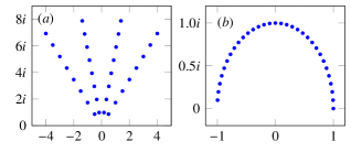
Figure 3: The figure depicts $\mathfrak{S}_{32}$ defined by (21), where the eigenvalues and the norming constants are shown in (a) and (b), respectively.

III Numerical Experiments: Test for Convergence and Complexity

III-A Secant-hyperbolic potential

A test for verifying the order of convergence and complexity can be readily designed using the well-known secant-hyperbolic potential given by $q(t)=A\operatorname{sech}{t}$, ($\kappa=-1$). The scattering coefficients are given by [12]

$$\begin{split}&a(\xi)=\frac{\left[\Gamma\left(0.5-i\xi\right)\right]^{2}}{\Gamma\left(A+0.5-i\xi\right)\Gamma\left(-A+0.5-i\xi\right)},\\ &b(\xi)=-\sin\pi A\operatorname{sech}\pi\xi,\end{split}$$ (16)

so that the reflection coefficient is given by $\rho(\xi)=b(\xi)/a(\xi)$. We set $A=4.4$. Let $\Omega_{h}=[-{\pi}/{2h},\,{\pi}/{2h}]$; then, the error in computing $b(\xi)$ is quantified by

$$e_{\text{rel.}}=\|b(\xi)-b_{N}(\xi)\|_{\mathsf{L}^{2}(\Omega_{h})}/\|b(\xi)\|_{\mathsf{L}^{2}(\Omega_{h})},$$ (17)

where the integrals are computed using the trapezoidal rule. Similar consideration applies to $\rho(\xi)$. For the purpose of benchmarking, we use the Split-Magnus (SM) and Magnus method with one-point Gauss quadrature (MG1) discussed in [5, Sec. IV]). Note that the complexity of SM is $\mathop{O}(N\log^{2}N)$ in computing the scattering coefficients while that of MG1 is $\mathop{O}(N^{2})$. The order of convergence for SM and MG1 both is $\mathop{O}(N^{-2})$. The numerical results are plotted in Fig. 2 where it is evident that $m$-step BDF (labeled BDF_m) as well as the $m$-step IA (labeled IA_m where IA₁ is identical to trapezoidal rule (TR)) schemes have better convergence rates with increasing $m$. The improved accuracy, however, comes at a price of increased complexity which is evidently not so prohibitive (besides, room for improvements in the implementation does exist). The IA methods are clearly superior to that of BDF in terms of accuracy while keeping the complexity same.

Figure 4: The figure shows a comparison of convergence behavior of NFT algorithms for computing the norming constant based on the discretization schemes, namely, BDF_m ($m\in\{1,2,3,4\}$), IA_m ($m\in\{1,2,3\}$), SM and MG1 (see Sec. III). The method IA₁ is identical to the trapezoidal rule (TR).

III-B Multisolitons

Arbitrary multisoliton solutions can be computed using the classical Darboux transformation (CDT), which allows us to test our algorithms for computing the norming constants. To this end, we define an arbitrary discrete spectrum and compute the corresponding multisoliton solution which serves as an input to the NFT algorithms. Let $b^{(\text{num.})}_{k}$ be the numerically computed approximation to $b_{k}$ which corresponds to the eigenvalue $\zeta_{k}$ which we assume to be known. The error in the norming constants can then be quantified by

$$e_{\text{rel}}=\sqrt{\left({\sum_{k=1}^{K}|b^{(\text{num.})}_{k}-b_{k}|^{2}}\right)\biggl{/}{\sum_{k=1}^{K}|b_{k}|^{2}}}.$$ (18)

For the discrete spectrum, the example chosen here is taken from [5] which can be described as follows: Define a sequence of angles for $J\in\mathbb{Z}_{+}$ by choosing $\Delta\theta=(\pi-2\theta_{0})/(J-1),\,\theta_{0}>0$, and $\theta_{j}=\theta_{0}+(j-1)\Delta\theta,\,j=1,2,\ldots,J$ so that $\theta_{j}\in[\theta_{0},\pi-\theta_{0}]$. Then the eigenvalues are chosen as

$$\zeta_{j+J(l-1)}=le^{i\theta_{j}},\,l=1,2,\ldots,8,\,j=1,2,\ldots,J.$$ (19)

Further, the norming constants are chosen as

$$b_{j}=e^{i\pi(j-1)/(8J-1)},\,j=1,2,\ldots,8J.$$ (20)

For this test, we set $\theta_{0}=\pi/3$ and $J=4$. Then we consider a sequence of discrete spectra defined as

$$\mathfrak{S}_{K}=\{(\zeta_{k},b_{k}),\,k=1,2,\ldots,K\},$$ (21)

where $K=4,8,\ldots,32$ (see Fig. 3). For fixed $K$, the eigenvalues are scaled by the scaling parameter $\kappa=2(\sum_{k=1}^{K}\operatorname{Im}\zeta_{k})^{1/2}$. Let $\eta_{\text{min}}=\min_{\{\zeta_{k}\}}\operatorname{Im}\zeta$, then the computational domain for this example is chosen as $[-T,\,T]$ where $T={22\kappa}/\eta_{\text{min}}$. The numerical results are plotted in Fig. 3 where it is evident that BDF_m as well as IA_m schemes have better convergence rates with increasing $m$. The IA methods are clearly superior to that of BDF in terms of accuracy.

IV Conclusion

In this letter we presented a family of fast NFT algorithms based on exponential linear multistep methods which were demonstrated to exhibit higher-order of convergence. Excluding the cost of computing the discrete eigenvalues, the proposed algorithms have a complexity of $\mathop{O}(KN+C_{p}N\log^{2}N)$ such that the error vanishes as $\mathop{O}(N^{-p})$ where $p\in\{1,2,3,4\}$ and $K$ is the number of eigenvalues. The form of $C_{p}$ depends on the underlying linear multistep method.

The future research in this direction will focus on developing compatible fast layer-peeling schemes for the discrete systems proposed in this letter so that higher-order convergent fast inverse NFT algorithms could be developed.

References

• [1] M. I. Yousefi and F. R. Kschischang, “Information transmission using the nonlinear Fourier transform, Part I,” IEEE Trans. Inf. Theory, vol. 60, no. 7, pp. 4312–4369, 2014.
• [2] S. K. Turitsyn, J. E. Prilepsky, S. T. Le, S. Wahls, L. L. Frumin, M. Kamalian, and S. A. Derevyanko, “Nonlinear Fourier transform for optical data processing and transmission: advances and perspectives,” Optica, vol. 4, no. 3, pp. 307–322, Mar 2017.
• [3] L. L. Frumin, A. A. Gelash, and S. K. Turitsyn, “New approaches to coding information using inverse scattering transform,” Phys. Rev. Lett., vol. 118, p. 223901, 2017.
• [4] A. Hasegawa and T. Nyu, “Eigenvalue communication,” J. Lightwave Technol., vol. 11, no. 3, pp. 395–399, Mar 1993.
• [5] V. Vaibhav, “Fast inverse nonlinear Fourier transformation using exponential one-step methods: Darboux transformation,” Phys. Rev. E, vol. 96, p. 063302, 2017.
• [6] V. Vaibhav and S. Wahls, “Introducing the fast inverse NFT,” in Optical Fiber Communication Conference.   Los Angeles, CA, USA: Optical Society of America, 2017, p. Tu3D.2.
• [7] V. Vaibhav, “Fast inverse nonlinear Fourier transformation,” 2017, arXiv:1706.04069[math.NA].
• [8] E. Hairer, S. P. Nørsett, and G. Wanner, Solving Ordinary Differential Equations I: Nonstiff Problems, ser. Springer Series in Computational Mathematics.   Berlin: Springer, 1993.
• [9] V. E. Zakharov and A. B. Shabat, “Exact theory of two-dimensional self-focusing and one-dimensional self-modulation of waves in nonlinear media,” Sov. Phys. JETP, vol. 34, pp. 62–69, 1972.
• [10] G. P. Agrawal, Nonlinear Fiber Optics, 3rd ed., ser. Optics and Photonics.   New York: Academic Press, 2013.
• [11] P. Henrici, “Fast Fourier methods in computational complex analysis,” SIAM Review, vol. 21, no. 4, pp. 481–527, 1979.
• [12] J. Satsuma and N. Yajima, “B. initial value problems of one-dimensional self-modulation of nonlinear waves in dispersive media,” Prog. Theor. Phys. Suppl., vol. 55, pp. 284–306, 1974.