Stable sets of certain non-uniformly hyperbolic horseshoes have the expected dimension

Abstract.

We show that the stable and unstable sets of non-uniformly hyperbolic horseshoes arising in some heteroclinic bifurcations of surface diffeomorphisms have the value conjectured in a previous work by the second and third authors of the present paper. Our results apply to first heteroclinic bifurcations associated to horseshoes with Hausdorff dimension $<22/21$ of conservative surface diffeomorphisms.

1. Introduction

In 2009, the second and third authors of the present paper proved in [5] that the semi-local dynamics of first heteroclinic bifurcations associated to “slightly thick” horseshoes of surface diffeomorphisms usually can be described by the so-called non-uniformly hyperbolic horseshoes.

In this article, we pursue the studies of Palis–Yoccoz [5] and Matheus–Palis [3] of the Hausdorff dimensions of the stable and unstable sets of non-uniformly hyperbolic horseshoes.

In order to state our main result (Theorem 1.4 below), we need first to recall the setting of Palis–Yoccoz work [5].

1.1. Heteroclinic bifurcations in Palis–Yoccoz regime

Fix a smooth diffeomorphism $g_{0}:M\to M$ of a compact surface $M$. Assume that $p_{s}$ and $p_{u}$ are periodic points of $g_{0}$ in distinct orbits such that $W^{s}(p_{s})$ and $W^{u}(p_{u})$ meet tangentially and quadratically at some point $q$. Suppose that $K$ is a horseshoe of $g_{0}$ such that $p_{s},p_{u}\in K$ and $q\in M\setminus K$, and, for some neighborhoods $U$ of $K$ and $V$ of the orbit $\mathcal{O}(q)$, the maximal invariant set of $U\cup V$ is $K\cup\mathcal{O}(q)$. In summary, $g_{0}$ has a first heteroclinic tangency at $q$ associated to periodic points $p_{s},p_{u}$ of a horseshoe $K$.

Let $(g_{t})_{|t|<t_{0}}$ be a $1$-parameter family of smooth diffeomorphisms of $M$ generically unfolding the first heteroclinic tangency of $g_{0}$ described in the previous paragraph. Assume that the continuations of $W^{s}(p_{s})$ and $W^{u}(p_{u})$ have no intersection near $q$ for $-t_{0}<t<0$ and two transverse intersections near $q$ for $0<t<t_{0}$.

Denote by $K_{g_{t}}:=\bigcap\limits_{n\in\mathbb{Z}}g_{t}^{-n}(U)$ hyperbolic continuation of $K$. In our context, it is not hard to describe the maximal invariant set

(1.1) $$\Lambda_{g_{t}}:=\bigcap\limits_{n\in\mathbb{Z}}g_{t}^{-n}(U\cup V)$$

in terms of $K_{g_{t}}$ when $-t_{0}<t\leq 0$: indeed, $\Lambda_{g_{t}}=K_{g_{t}}$ when $-t_{0}<t<0$, and $\Lambda_{g_{0}}=K\cup\mathcal{O}(q)$.

On the other hand, the study of $\Lambda_{g_{t}}$ for $0<t<t_{0}$ represents an important challenge when the Hausdorff dimension of the initial horseshoe $K=K_{g_{0}}$ is larger than one.

In their paper [5], Palis and Yoccoz studied strongly regular parameters $0<t<t_{0}$ whenever $K_{g_{0}}$ is slightly thick, i.e.,

(1.2) $$(d_{s}^{0}+d_{u}^{0})^{2}+(\max\{d_{s}^{0},d_{u}^{0}\})^{2}<(d_{s}^{0}+d_{u}^{0})+\max\{d_{s}^{0},d_{u}^{0}\}$$

where $d_{s}^{0}$ and $d_{u}^{0}$ (resp.) are the transverse Hausdorff dimensions of the invariant sets $W^{s}(K_{g_{0}})$ and $W^{u}(K_{g_{0}})$ (resp.). In this setting, Palis and Yoccoz proved that any strongly regular parameter $t$ has the property that $\Lambda_{g_{t}}$ is a non-uniformly hyperbolic horseshoe, and, moreover, the strongly regular parameters are abundant near $t=0$:

$$\lim\limits_{\varepsilon\to 0^{+}}\frac{1}{\varepsilon}\textrm{Leb}_{1}(\{0<t<\varepsilon:t\textrm{ is a strongly regular parameter}\})=1$$

(Here $\textrm{Leb}_{1}$ is the $1$-dimensional Lebesgue measure.)

Remark 1.1.

This result of Palis and Yoccoz is a semi-local dynamical result: indeed, Appendix A below (by the C. G. Moreira and the first two authors of this paper) shows that it is often the case that $U\cup V$ can be chosen of almost full Lebesgue measure.

We refer the reader to the original paper [5] for the precise definitions of strongly regular parameters and non-uniformly hyperbolic horseshoes. For the purposes of this article, we will discuss some features of non-uniformly hyperbolic horseshoes in Section 2 below.

For the time being, we recall only that non-uniformly hyperbolic horseshoes are saddle-like sets:

Theorem 1.2 (cf. Theorem 6 in [5] and Theorem 1.2 in [3]).

Under the previous assumptions, if $t$ is a strongly regular parameter, then

$$\textrm{HD}(W^{s}(\Lambda_{g_{t}}))<2\quad\textrm{ and }\quad\textrm{HD}(W^{u}(\Lambda_{g_{t}}))<2$$

where HD stands for the Hausdorff dimension. In particular, $\Lambda_{g_{t}}$ does not contain attractors nor repellors.

As it turns out, this result leaves open the exact calculation of the quantitites $\textrm{HD}(W^{s}(\Lambda_{g_{t}}))$: in fact, Palis and Yoccoz conjectured in [5, p. 14] that the stable sets of non-uniformly hyperbolic horseshoes have Hausdorff dimensions very close or perhaps equal to the expected dimension $1+d_{s}$, where $d_{s}$ is a certain number close to $d_{s}^{0}$ measuring the transverse dimension of the stable set of the “main non-uniformly hyperbolic part” of $\Lambda_{g_{t}}$.

Remark 1.3.

The proof of Theorem 1.2 never allows to show that $W^{s}(\Lambda_{g_{t}})$ has the expected dimension: see Remark 8 of [3].

In this article, we give the following (partial) answer to this conjecture.

1.2. Statement of the main theorem

We show that the conjecture stated above is true at least when the transverse dimensions $d_{s}^{0}$ and $d_{u}^{0}$ of the stable and unstable sets of the initial horseshoe $K_{g_{0}}$ satisfy a stronger constraint than (1.2) above.

Theorem 1.4.

In the same setting of Theorem 1.2, denote by

$$\beta^{*}(d_{s}^{0},d_{u}^{0}):=\frac{(1-\min\{d_{s}^{0},d_{u}^{0}\})(d_{s}^{0}+d_{u}^{0})}{\max\{d_{s}^{0},d_{u}^{0}\}(\max\{d_{s}^{0},d_{u}^{0}\}+d_{s}^{0}+d_{u}^{0}-1)}$$

In addition to (1.2) (i.e., $\beta^{*}(d_{s}^{0},d_{u}^{0})>1$), let us also assume that the transverse dimensions $d_{s}^{0}$ and $d_{u}^{0}$ of the stable and unstable sets of the initial horseshoe $K_{g_{0}}$ satisfy

(1.3) $$\beta^{*}(d_{s}^{0},d_{u}^{0})\leq 1+\min\left\{\frac{-\log|\lambda(p_{s})|}{\log|\mu(p_{s})|},\frac{\log|\mu(p_{u})|}{-\log|\lambda(p_{u})|}\right\}$$

where $\lambda(p_{\alpha})$, resp. $\mu(p_{\alpha})$, is the stable, resp. unstable, eigenvalue of the periodic point $p_{\alpha}$ for $\alpha=s,u$, and

(1.4) $$\beta^{*}(d_{s}^{0},d_{u}^{0})>\frac{5}{3}$$

Then, for any strongly regular parameter $t$, one has

$$\textrm{HD}(W^{s}(\Lambda_{g_{t}}))=1+d_{s}$$

where $0<d_{s}=d_{s}(g_{t})<1$ is a certain quantity close to $d_{s}^{0}$ given by the transverse dimensions of the lamination $\widetilde{\mathcal{R}}^{\infty}_{+}$ of stable curves associated to the well-behaved parts of $\Lambda_{g_{t}}$ (see pages 12, 13 and 14 of [5]).

Remark 1.5.

Analogously to [5], there is a symmetry between past and future in our arguments. Thus, the analog of Theorem 1.4 for the unstable set $W^{u}(\Lambda_{g_{t}})$ holds after exchanging the roles of $d_{s}^{0}$ and $d_{u}^{0}$, etc.

Remark 1.6.

Of course, we believe that the conditions (1.3) and (1.4) are not necessary for the validity of the conclusion of Theorem 1.4, but our proof of this result in Section 3 below does not allow us to bypass these technical conditions. We hope to come back to this issue in the future.

Remark 1.7.

The condition (1.3) is automatic in the conservative case (when $g_{0}$ preserves a smooth area form). Indeed, the multipliers $\lambda(p_{\alpha})$ and $\mu(p_{\alpha})$ verify $\lambda(p_{\alpha})\mu(p_{\alpha})=1$ in this situation, so that (1.3) becomes the requirement $\beta^{*}(d_{s}^{0},d_{u}^{0})\leq 2$ which is always true when $d_{s}^{0}+d_{u}^{0}>1$.

Similarly, the condition (1.3) is automatic if $K_{g_{0}}$ is a product of two affine Cantor sets $K^{s}$ and $K^{u}$ of the real line obtained from affine maps with constant dilatations $1/\lambda>1$ and $\mu>1$ sending two finite collections of $\ell\in\mathbb{N}$ disjoint closed subintervals of $[0,1]$ surjectively on their convex hull $[0,1]$. In fact, it is well-known that the transverse Hausdorff dimensions of such a horseshoe $K_{g_{0}}$ are $d_{s}^{0}=\log\ell/\log(1/\lambda)$ and $d_{u}^{0}=\log\ell/\log\mu$, so that the requirement (1.3) becomes

$$\beta^{*}(d_{s}^{0},d_{u}^{0}) \leq 1+\min\left\{\frac{\log(1/\lambda)}{\log\mu},\frac{\log\mu}{\log(1/\lambda)}\right\}=1+\min\left\{\frac{d_{s}^{0}}{d_{u}^{0}},\frac{d_{u}^{0}}{d_{s}^{0}}\right\}$$

$$= \frac{d_{s}^{0}+d_{u}^{0}}{\max\{d_{s}^{0},d_{u}^{0}\}}$$

which is always valid when $d_{s}^{0}+d_{u}^{0}>1$.

In summary, it is “often” the case that the condition (1.3) is less restrictive than the condition (1.4) in “many” applications of Theorem 1.4.

Remark 1.8.

A natural question closely related to the statement of Theorem 1.4 is: given a strongly regular parameter $t$, what is the Hausdorff dimension of the non-uniformly hyperbolic horseshoe $\Lambda_{g_{t}}$ itself? Of course, it is reasonable to conjecture that a non-uniformly hyperbolic horseshoe $\Lambda_{g_{t}}$ has the “expected” dimension $HD(\Lambda_{g_{t}})=d_{s}+d_{u}$. In this direction, let us observe that Theorem 1.4 implies only that $HD(\Lambda_{g_{t}})\leq 1+\min\{d_{s},d_{u}\}$ (since $\Lambda_{g_{t}}=W^{s}(\Lambda_{g_{t}})\cap W^{u}(\Lambda_{g_{t}})$), but this is still far from the “expected” value (as $d_{s}+d_{u}<1+\min\{d_{s},d_{u}\}$). We plan to address elsewhere the question of computing $HD(\Lambda_{g_{t}})$ for strongly regular parameters $t$.

For the sake of comparison of the conditions (1.2) and (1.4), we plotted below (using Mathematica) the portions of the regions

$$\mathcal{D}=\{(d_{s}^{0},d_{u}^{0})\in[0,1]\times[0,1]:(d_{s}^{0},d_{u}^{0})\textrm{ satisfies }\eqref{e.Dset}\}$$

and

$$\mathcal{PY}=\{(d_{s}^{0},d_{u}^{0})\in[0,1]\times[0,1]:(d_{s}^{0},d_{u}^{0})\textrm{ satisfies }\eqref{e.PYset}\}$$

below the diagonal $\Delta=\{(d_{s}^{0},d_{u}^{0})\in\mathbb{R}^{2}:1/2<d_{s}^{0}=d_{u}^{0}<1\}$.

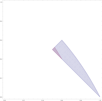
Figure 1. $\mathcal{D}$ (in red) inside $\mathcal{PY}$ (in blue).

We have $\mathcal{D}$ occupies slightly more than $3\%$ of $\mathcal{PY}$:

$$\frac{\textrm{area}(D)}{\textrm{area}(\mathcal{PY})}=0.030136...$$

These regions intersect the diagonal segment

$$\Delta=\{(d_{s}^{0},d_{u}^{0})\in\mathbb{R}^{2}:1/2<d_{s}^{0}=d_{u}^{0}<1\}$$

along

$$\mathcal{PY}\cap\Delta=\{(d_{s}^{0},d_{u}^{0})\in\mathbb{R}^{2}:1/2<d_{s}^{0}=d_{u}^{0}<3/5\}$$

and

$$\mathcal{D}\cap\Delta=\{(d_{s}^{0},d_{u}^{0})\in\mathbb{R}^{2}:1/2<d_{s}^{0}=d_{u}^{0}<11/21\}.$$

Remark 1.9.

The symmetry in Remark 1.5 actually implies that $HD(W^{s}(g_{t}))=1+d_{s}$ and $HD(W^{u}(g_{t}))=1+d_{u}$ if $t$ is a strongly regular parameter, $(d_{s}^{0},d_{u}^{0})$ satisfy (1.3), and $(d_{s}^{0},d_{u}^{0})$ belongs to the region $\mathcal{D}$.

1.3. Outline of the proof of the main result

Recall from Palis–Yoccoz paper [5] that the stable set $W^{s}(\Lambda)$ of a non-uniformly hyperbolic horseshoe $\Lambda$ can be written as the disjoint union of an exceptional part $\mathcal{E}^{+}$ and a lamination with $C^{1+Lip}$-leaves and Lipschitz holonomy with transverse Hausdorff dimension $0<d_{s}<1$ is close to the stable dimension $d_{s}^{0}$ of the initial horseshoe $K_{g_{0}}$.

Hence, the proof of Theorem 1.4 is reduced to show that the Hausdorff dimension of the exceptional part $\mathcal{E}^{+}$ of $W^{s}(\Lambda)$ is $HD(\mathcal{E}^{+})<1+d_{s}$.

By definition, the points of $\mathcal{E}^{+}$ visit a sequence of “strips” $(P_{k})_{k\in\mathbb{N}}$ whose “widths” decay doubly exponentially fast (cf. Lemma 24 of [5]). In particular, by fixing $k\in\mathbb{N}$ large and by decomposing the strip $P_{k}$ into squares, we obtain a covering of very small diameter of the image of $\mathcal{E}^{+}$ under some positive iterate of the dynamics.

It was shown in [3] that the covering of the images of $\mathcal{E}^{+}$ in the previous paragraph can be used to prove that $HD(\mathcal{E}^{+})<2$. More concretely, the negative iterates of the dynamics take the covering of $P_{k}$ back to $\mathcal{E}^{+}$ while alternating between affine-like (hyperbolic) iterates and a fixed folding map. In principle, the folding effect accumulates very quickly, but if we ignore the action of folding map by replacing all “parabolic shapes” by “fat strips”, then we obtain a cover of $\mathcal{E}^{+}$ with small diameter and controlled cardinality thanks to the double exponential decay of $P_{j}$’s. As it turns out, this suffices to establish $HD(\mathcal{E}^{+})<2$, but this strategy does not yield $HD(\mathcal{E}^{+})<1+d_{s}$ (cf. Remark 1.3 above).

For this reason, during the proof of Theorem 1.4, we do not completely ignore the “parabolic shapes” mentioned above. In fact, we estimate the contribution of the parabolic shapes inside the $P_{j}$’s to the Hausdorff dimension of $\mathcal{E}^{+}$ in terms of the derivative and Jacobian of the dynamics thanks to an analytical lemma (cf. Lemma 3.4 below) saying that the Hausdorff measure of scale $1$ of the image $f(\mathbb{D}^{2})$ of the unit disk $\mathbb{D}^{2}=\{(x,y)\in\mathbb{R}^{2}:x^{2}+y^{2}\leq 1\}$ under a $C^{1}$-map $f:\mathbb{D}^{2}\to\mathbb{R}^{2}$ is bounded by interpolation of the $C^{0}$-norms of the derivative and Jacobian of $f$. Also, we prove that this estimate is sufficient to derive $HD(\mathcal{E}^{+})<1+d_{s}$ when the double exponential rate of decays of widths of $P_{j}$’s is adequate (namely, (1.4) holds). Furthermore, we prove the analytical lemma by decomposing dyadically $f(\mathbb{D}^{2})$ and by interpreting the $d$-Hausdorff measure of $f(\mathbb{D}^{2})$ as a $L^{d}$-norm. In this way, for $1<d<2$, we can estimate this $L^{d}$-norm by interpolation between certain $L^{1}$ and $L^{2}$ norms that are naturally controlled by the derivatives and Jacobians of $f$.

In summary, the novelty in the proof of Theorem 1.4 (in comparison with Theorem 1.2) is the application of the analytical lemma described above to control the Hausdorff measure of $\mathcal{E}^{+}$.

Remark 1.10.

Similarly to [3], our main result holds for the same strongly regular parameters of Palis-Yoccoz [5].

Remark 1.11.

The arguments outlined above provide sequences of good coverings of the stable and unstable sets $W^{s}(\Lambda)$ and $W^{u}(\Lambda)$ permitting to calculate their Hausdorff dimensions. However, in relation with Remark 1.8 above, let us observe that it is not obvious how to combine these sequences to produce good coverings of the non-uniformly hyperbolic horseshoe $\Lambda$ itself allowing to compute its Hausdorff dimension. In fact, the naive idea of taking intersections of elements of coverings of $W^{s}(\Lambda)$ and $W^{u}(\Lambda)$ in order to produce a cover of $\Lambda=W^{s}(\Lambda)\cap W^{u}(\Lambda)$ does not work directly because of the possible “lack of transversality” (especially near $\mathcal{E}^{+}\cap\mathcal{E}^{-}$) that allows for a potentially bad geometry of such coverings of $\Lambda$.

1.4. Organization of the paper

We divide the remainder of this article into two parts. In Section 2, we recall some facts from Palis–Yoccoz article [5]. In Section 3, we prove an analytical lemma (cf. Lemma 3.4) about Hausdorff measures of planar sets and we apply it to get Theorem 1.4.

Acknowledgments

We are grateful to the following institutions for their hospitality during the preparation of this article: Collège de France, Instituto de Matemática Pura e Aplicada (IMPA), and Kungliga Tekniska högskolan (KTH). The authors were partially supported by the Balzan Research Project of J. Palis, the French ANR grant “DynPDE” (ANR-10-BLAN 0102) and the Brazilian CAPES grant (88887.136371/2017-00).

2. Preliminaries

In this section, we review some basic properties of the non-uniformly horseshoes introduced in [5] (see also Section 2 of [3]).

2.1. Strongly regular parameters

Let $0<\varepsilon_{0}\ll\tau\ll 1$ be two very small constants, and define a sequence of scales $\varepsilon_{k+1}=\varepsilon_{k}^{1+\tau}$, $k\in\mathbb{N}$. The inductive scheme in [5] defining the strongly regular parameters goes as follows. The initial candidate interval is $I_{0}=[\varepsilon_{0},2\varepsilon_{0}]$. The $k$th step of induction consists in dividing the selected candidate intervals of the previous step into $\lfloor\varepsilon_{k}^{-\tau}\rfloor$ disjoint candidates of lengths $\varepsilon_{k+1}$. These new candidates are submitted to a strong regularity test and we select for the $(k+1)$th step of induction only the candidates passing this test.

By definition, $t\in I_{0}=[\varepsilon_{0},2\varepsilon_{0}]$ is strongly regular parameter whenever $\{t\}=\bigcap\limits_{k\in\mathbb{N}}I_{k}$ where $I_{0}\supset\dots\supset I_{k}\supset\dots$ are selected candidate intervals.

The strong regularity tests are relevant for two reasons (at least). Firstly, they are rich enough to ensure several nice properties of “non-uniform hyperbolicity” of $\Lambda_{g_{t}}$ for strongly regular parameters $t\in I_{0}$. Secondly, they are sufficiently flexible to allow the presence of many strongly regular parameters: by Corollary 15 of [5], the set of strongly regular parameters $t\in I_{0}=[\varepsilon_{0},2\varepsilon_{0}]$ has Lebesgue measure $\geq\varepsilon_{0}(1-3\varepsilon_{0}^{\tau^{2}})$.

The notion of strong regularity tests is intimately related to an adequate class $\mathcal{R}(I)$ of affine-like iterates attached to each candidate interval $I$.

In the next three subsections, we briefly recall the construction of $\mathcal{R}(I)$.

2.2. Semi-local dynamics of heteroclinic bifurcations

We fix geometrical Markov partitions of the horseshoes $K_{g_{t}}$ depending smoothly on $g_{t}$. In other terms, we choose a finite system of smooth charts $I_{a}^{s}\times I_{a}^{u}\to R_{a}\subset M$ indexed by a finite alphabet $a\in\mathcal{A}$ with the properties that these charts depend smoothly on $g_{t}$, the intervals $I_{a}^{s}$ and $I_{a}^{u}$ are compact, the rectangles $R_{a}$ are disjoint, and the horseshoe $K_{g_{t}}$ is the maximal invariant set of the interior of $R:=\bigcup\limits_{a\in\mathcal{A}}R_{a}$, the family $(K_{g_{t}}\cap R_{a})_{a\in\mathcal{A}}$ is a Markov partition of $K_{g_{t}}$. Moreover, we assume that no rectangle meets the orbits of $p_{s}$ and $p_{u}$ at the same time.

Remark 2.1.

The intervals $I_{a}^{s}=[x_{a}^{-},x_{a}^{+}]$, $I_{a}^{u}=[y_{a}^{-},y_{a}^{+}]$, $a\in\mathcal{A}$, above can be replaced by slightly larger intervals $J_{a}^{s}=[x_{a}^{-}-C^{-1},x_{a}^{+}+C^{-1}]$, $J_{a}^{u}=[y_{a}^{-}-C^{-1},y_{a}^{+}+C^{-1}]$ (where $C=C(g_{0})\geq 1$ is a large constant) without changing any of the properties in the previous paragraph. This fact will be used later during the discussion of affine-like iterates.

The Markov partition $(K_{g_{t}}\cap R_{a})_{a\in\mathcal{A}}$ allows to topologically conjugate the dynamics of $g_{t}$ on $K_{g_{t}}$ and the subshift of finite type of $\mathcal{A}^{\mathbb{Z}}$ with transitions

$$\mathcal{B}:=\{(a,a^{\prime})\in\mathcal{A}^{2}:g_{0}(R_{a})\cap R_{a^{\prime}}\cap K_{g_{0}}\neq\emptyset\}.$$

Furthermore, for each $g_{t}$ with $t>0$, we have a compact lenticular region $L_{u}\subset R_{a_{u}}$ (near the initial heteroclinic tangency point $q\in M\setminus K$ of $g_{0}$) bounded by a piece of the unstable manifold of $p_{u}$ and a piece of the stable manifold of $p_{s}$. Moreover, $L_{u}$ moves outside $R$ for $N_{0}-1$ iterates of $g_{t}$ before entering $R$ (for some integer $N_{0}=N_{0}(g_{0})\geq 2$) because no rectangle meets both orbits of $p_{s}$ and $p_{u}$. The image $L_{s}=g_{t}^{N_{0}}(L_{u})$ of $L_{u}$ under $G:=g_{t}^{N_{0}}|_{L_{u}}$ defines another lenticular region $L_{s}\subset R_{a_{s}}$ and the regions $g^{i}(L_{u})$, $0\leq i\leq N_{0}$ are called parabolic tongues.

Let $\widehat{R}:=R\cup\bigcup\limits_{0<i<N_{0}}g^{i}(L_{u})$. By definition, the set $\Lambda_{g}$ introduced in (1.1) is the maximal invariant set of $\widehat{R}$, i.e., $\Lambda_{g_{t}}=\bigcap\limits_{n\in\mathbb{Z}}g_{t}^{-n}(\widehat{R})$.

The dynamics of $g_{t}$ on $\widehat{R}$ is driven by the transition maps

$$g_{aa^{\prime}}=g_{t}|_{R_{a}\cap g^{-1}(R_{a^{\prime}})}:R_{a}\cap g_{t}^{-1}(R_{a^{\prime}})\to g_{t}(R_{a})\cap R_{a^{\prime}},\quad(a,a^{\prime})\in\mathcal{B},$$

related to the Markov partition $R$, and the folding map $G=g_{t}^{N_{0}}|_{L_{u}}:L_{u}\to L_{s}$ between the parabolic tongues.

Qualitatively speaking, the transitions $g_{aa^{\prime}}$ correspond to “affine” hyperbolic maps: for our choices of charts, $g_{aa^{\prime}}$ contracts “almost vertical” directions and expands “almost horizontal” directions. Of course, this hyperbolic structure can be destroyed by the folding map $G$ and this phenomenon is the source of non-hyperbolicity of $\Lambda_{g_{t}}$.

For this reason, the notion of non-uniformly hyperbolic horseshoes is defined in [5] in terms of a certain “affine-like” iterates of $g_{t}$. Before entering into this discussion, let us quickly overview the notion of affine-like maps.

2.3. Generalities on affine-like maps

Let $I_{0}^{s},I_{0}^{u},I_{1}^{s}$ and $I_{1}^{u}$ be compact intervals with coordinates $x_{0},y_{0},x_{1}$ and $y_{1}$. A diffeomorphism $F$ from a vertical strip

$$P:=\{(x_{0},y_{0}):\varphi^{-}(y_{0})\leq x_{0}\leq\varphi^{+}(y_{0})\}\subset I_{0}^{s}\times I_{0}^{u}$$

onto a horizontal strip

$$Q:=\{(x_{1},y_{1}):\psi^{-}(x_{1})\leq y_{1}\leq\psi^{+}(x_{1})\}\subset I_{1}^{s}\times I_{1}^{u}$$

is affine-like whenever the projection from the graph of $F$ to $I_{0}^{u}\times I_{1}^{s}$ is a diffeomorphism onto $I_{0}^{u}\times I_{1}^{s}$.

By definition, an affine-like map $F$ has an implicit representation $(A,B)$, i.e., there are smooth maps $A$ and $B$ on $I_{0}^{u}\times I_{1}^{s}$ such that $F(x_{0},y_{0})=(x_{1},y_{1})$ if and only if $x_{0}=A(y_{0},x_{1})$ and $y_{1}=B(y_{0},x_{1})$.

For our purposes, we shall consider exclusively affine-like maps satisfying a cone condition and a distortion estimate. More concretely, let $\lambda>1$, $u_{0}>0$, $v_{0}>0$ with $1<u_{0}v_{0}\leq\lambda^{2}$ and $D_{0}>0$ be the constants fixed in page 32 of [5]: their choices depend solely on $g_{0}$.

An affine-like map $F(x_{0},y_{0})=(x_{1},y_{1})$ with implicit representation $(A,B)$ satisfies a $(\lambda,u,v)$ cone condition if

$$\lambda|A_{x}|+u_{0}|A_{y}|\leq 1\quad\textrm{ and }\quad\lambda|B_{y}|+v_{0}|B_{x}|\leq 1$$

where $A_{x},A_{y},B_{x},B_{y}$ are the first order partial derivatives of $A$ and $B$. Also, an affine-like map $F(x_{0},y_{0})=(x_{1},y_{1})$ with implicit representation $(A,B)$ satisfies a $2D_{0}$ distortion condition if

$$\partial_{x}\log|A_{x}|,\partial_{y}\log|A_{x}|,A_{yy},\partial_{y}\log|B_{y}|,\partial_{x}\log|B_{y}|,B_{xx}$$

are uniformly bounded by $2D_{0}$.

Remark 2.2.

The widths of the domain $P$ and the image $Q$ of an affine-like map $F:P\to Q$ with implicit representation $(A,B)$ are

$$|P|:=\max|A_{x}|\quad\textrm{and}\quad|Q|:=\max|B_{y}|$$

The widths satisfy $|P|\leq C\min|A_{x}|$ and $|Q|\leq C\min|B_{y}|$ where $C=C(g_{0})\geq 1$.

The transitions $g_{aa^{\prime}}$ associated to the Markov partition $R$ of the horseshoe $K_{g_{t}}$ are affine-like maps satisfying the cone and distortion conditions with parameters $(\lambda,u_{0},v_{0},2D_{0})$: see Subsection 3.4 of [5].

Moreover, we can build new affine-like maps using the so-called simple and parabolic compositions of two affine-like maps.

Given compact intervals $I_{j}^{s},I_{j}^{u}$, $j=0,1,2$, and two affine-like maps $F:P\to Q$ and $F^{\prime}:P^{\prime}\to Q^{\prime}$ with domains $P\subset I_{0}^{s}\times I_{0}^{u}$ and $P^{\prime}\subset I_{1}^{s}\times I_{1}^{u}$ and images $Q\subset I_{1}^{s}\times I_{1}^{u}$ and $Q^{\prime}\subset I_{2}^{s}\times I_{2}^{u}$ satisfying the $(\lambda,u_{0},v_{0})$ cone condition, the map $F^{\prime\prime}=F^{\prime}\circ F$ from $P^{\prime\prime}=P\cap F^{-1}(P^{\prime})$ to $Q^{\prime\prime}=Q\cap P^{\prime}$ is an affine-like map satisfying the $(\lambda^{2},u_{0},v_{0})$ cone condition (see Subsection 3.3 of [5]). The map $F^{\prime\prime}$ is the simple composition of $F$ and $F^{\prime}$.

Given compact intervals $I_{j}^{s},I_{j}^{u}$, $j=0,1$, and two affine-like maps $F_{0}:P_{0}\to Q_{0}$, $F_{1}:P_{1}\to Q_{1}$ from vertical strips $P_{0}\subset I_{0}^{s}\times I_{0}^{u}$, $P_{1}\subset I_{a_{s}}^{s}\times I_{a_{s}}^{u}$ to horizontal strips $Q_{0}\subset I_{a_{u}}^{s}\times I_{a_{u}}^{u}$, $Q_{1}\subset I_{1}^{s}\times I_{1}^{u}$, we can introduce a quantity $\delta(Q_{0},P_{1})$ roughly measuring the distance between $Q_{0}$ and the tip of the parabolic strip $G^{-1}(P_{1})$ (where $G$ is the folding map): see Subsection 3.5 of [5]. If

$$\delta(Q_{0},P_{1})>(1/b)(|P_{1}|+|Q_{0}|)$$

and the implicit representations of $F_{0}$ and $F_{1}$ to satisfy the bound

$$\max\{|(A_{1})_{y}|,|(A_{1})_{yy}|,|(B_{0})_{x}|,|(B_{0})_{xx}|\}<b$$

for an adequate constant $b=b(g_{0})>0$, the composition $F_{1}\circ G\circ F_{0}$ defines two affine-like maps $F^{\pm}:P^{\pm}\to Q^{\pm}$ with domains $P^{\pm}\subset P_{0}$ and $Q^{\pm}\subset Q_{1}$ called the parabolic compositions of $F_{0}$ and $F_{1}$.

2.4. The class $\mathcal{R}(I)$ of certain affine-like iterates

Given a parameter interval $I\subset[\varepsilon_{0},2\varepsilon_{0}]$, a triple $(P,Q,n)=(P_{t},Q_{t},n)_{t\in I}$ is called a $I$-persistent affine-like iterate if $P_{t}\subset R_{a}$, resp. $Q_{t}\subset R_{a^{\prime}}$, is a vertical, resp. horizontal, strip varying smoothly with $t\in I$, $n\geq 0$ is an integer such that $g_{t}^{n}|_{P_{t}}:P_{t}\to Q_{t}$ is an affine-like map for all $t\in I$, and $g_{t}^{m}(P_{t})\subset\widehat{R}$ for each $0\leq m\leq n$.

Given a candidate parameter interval $I$, it is assigned in Subsection 5.3 of [5] a class $\mathcal{R}(I)$ of certain $I$-persistent affine-like iterates verifying seven requirements (R1) to (R7):

• the transitions $g_{aa^{\prime}}:R_{a}\cap g_{t}^{-1}(R_{a^{\prime}})\to g_{t}(R_{a})\cap R_{a^{\prime}}$, $(a,a^{\prime})\in\mathcal{B}$, belong to $\mathcal{R}(I)$,

• each $(P,Q,n)\in\mathcal{R}(I)$ is a $I$-persistent affine-like iterate satisfying the $(\lambda,u_{0},v_{0})$ cone condition and the $2D_{0}$ distortion condition,

• the class $\mathcal{R}(I)$ is stable under simple compositions,

• denote by $P_{s}$, resp. $Q_{u}$, the smallest cylinder of the Markov partition of $K_{g_{t}}$ containing $L_{s}$, resp. $L_{u}$; if $(P,Q,n)\in\mathcal{R}(I)$ and $P\subset P_{s}$, then $|A_{y}|,|A_{yy}|\leq C\varepsilon_{0}$ for all $t\in I$; similarly, if $(P,Q,n)\in\mathcal{R}(I)$ and $Q\subset Q_{u}$, then $|B_{x}|,|B_{xx}|\leq C\varepsilon_{0}$ for all $t\in I$,

• the class $\mathcal{R}(I)$ is stable under certain allowed parabolic compositions (cf. page 33 of [5]),

• each $(P,Q,n)\in\mathcal{R}(I)$ with $n>1$ is obtained from simple or allowed parabolic compositions of shorter elements,

• if the parabolic composition of $(P_{0},Q_{0},n_{0}),(P_{1},Q_{1},n_{1})\in\mathcal{R}(I)$ is allowed, then

  $$\delta(Q_{0},P_{1})\geq(1/C)(|P_{1}|^{1-\eta}+|Q_{0}|^{1-\eta})$$

  where $\delta(Q_{0},P_{1})$ is the distance between $Q_{0}$ and the tip of $G^{-1}(P_{1})$, $C=C(g_{0})\geq 1$, and the parameter $\eta$ relates to $\varepsilon_{0}$ and $\tau$ via the condition $0<\varepsilon_{0}\ll\eta\ll\tau<1$.

Furthermore, Theorem 1 of [5] ensures that the class $\mathcal{R}(I)$ satisfying (R1) to (R7) above is unique.

For technical reasons, we will need to work with extensions of the elements $\mathcal{R}(I)$. More concretely, we consider the intervals $J^{s}_{a}$, $J^{u}_{a}$ from Remark 2.1 and we denote by $S:=\bigcup\limits_{a\in\mathcal{A}}S_{a}$ the geometric Markov partition associated to smooth charts $J_{a}^{s}\times J_{a}^{u}\to S_{a}$. We say that $(\widetilde{P},\widetilde{Q},n)$ extends $(P,Q,n)\in\mathcal{R}(I)$ if $(\widetilde{P},\widetilde{Q},n)$ is an affine-like map with respect to $S$ satisfying the $(\lambda,u_{0},v_{0})$ cone condition and the $3D_{0}$ distortion condition such that the restriction of $(\widetilde{P},\widetilde{Q},n)$ to $R$ is $(P,Q,n)$. Note that if $(\widetilde{P},\widetilde{Q},n)$ extends $(P,Q,n)$, then $\widetilde{P}$ is a strip of width $\leq C|P|$ containing a $C^{-1}|P|$-neighborhood of $P$ and $\widetilde{Q}$ is a strip of width $\leq C|Q|$ containing a $C^{-1}|Q|$-neighborhood of $Q$ (where $C=C(g_{0})\geq 1$) thanks to the cone and distortion conditions.

Proposition 2.3.

Each element $(P,Q,n)\in\mathcal{R}(I)$ admits an extension.

Proof.

Consider the subclass $\mathcal{S}(I)$ of $\mathcal{R}(I)$ consisting of elements admitting an extension. We want to show that $\mathcal{S}(I)=\mathcal{R}(I)$, and, in view of Theorem 1 of [5], it suffices to check that $\mathcal{S}(I)$ verifies the requirements (R1) to (R7).

The fact that the transitions $g_{aa^{\prime}}$ can be extended was already observed in Remark 2.1. In particular, $\mathcal{S}(I)$ satisfies (R1).

The requirements (R2), (R4) and (R7) for $\mathcal{S}(I)$ are automatic (because they concern geometric properties of $(P,Q,n)\in\mathcal{S}(I)\subset\mathcal{R}(I)$ themselves).

The condition (R3) for $\mathcal{S}(I)$ holds because the simple composition of $(P_{0},Q_{0},n_{0}),(P_{1},Q_{1},n_{1})\in\mathcal{S}(I)$ is extended by the simple composition of the extensions of $(P_{0},Q_{0},n_{0})$ and $(P_{1},Q_{1},n_{1})$.

If $(P_{0},Q_{0},n_{0}),(P_{1},Q_{1},n_{1})\in\mathcal{S}(I)$ satisfy the transversality requirement $Q_{0}\pitchfork_{I}P_{1}$ (from page 34 of [5]) allowing parabolic composition, then their extensions $(\widetilde{P}_{0},\widetilde{Q}_{0},n_{0}),(\widetilde{P}_{1},\widetilde{Q}_{1},n_{1})$ verify the same transversality requirement after replacing the constant $2$ in (T1), (T2), (T3) in page 34 of [5] by $7/4$. From this fact and the discussion of parabolic compositions in Subsections 3.5 and 3.6 of [5], one sees that the parabolic composition of $(\widetilde{P}_{0},\widetilde{Q}_{0},n_{0})$ and $(\widetilde{P}_{1},\widetilde{Q}_{1},n_{1})$ is an extension of the parabolic composition of $(P_{0},Q_{0},n_{0})$ and $(P_{1},Q_{1},n_{1})\in\mathcal{S}(I)$. Therefore, $\mathcal{S}(I)$ satisfies (R5).

At this point, it remains to check (R6) for $\mathcal{S}(I)$. For this sake, we recall (from Subsection 5.5 of [5]) that $\mathcal{R}(I_{0})$ consist of all affine-like iterates associated to the horseshoe $K_{g_{t}}$. In particular, $\mathcal{S}(I_{0})=\mathcal{R}(I_{0})$ thanks to our discussion so far. On the other hand, if $I$ is a candidate interval distinct from $I_{0}$ and $\mathcal{S}(\widetilde{I})=\mathcal{R}(\widetilde{I})$ for the smallest candidate interval $\widetilde{I}$ containing $I$, then we can apply the structure theorem (cf. Theorem 2 of [5]) to write any element $(P,Q,n)\in\mathcal{R}(I)$ not coming from $\mathcal{R}(\widetilde{I})$ as the allowed parabolic compositions of shorter elements $(P_{0},Q_{0},n_{0}),\dots,(P_{k},Q_{k},n_{k})\in\mathcal{R}(\widetilde{I})$, $k>0$. Since $\mathcal{S}(\widetilde{I})=\mathcal{R}(\widetilde{I})$, we conclude that $\mathcal{S}(I)$ verifies (R6). ∎

2.5. Strong regularity tests

A candidate parameter interval $I$ is tested for several quantitative conditions on the family of so-called bicritical elements of $\mathcal{R}(I)$. If a candidate interval $I$ passes this strong regularity test, then all bicritical elements $(P,Q,n)\in\mathcal{R}(I)$ are thin in the sense that

$$|P|<|I|^{\beta},\quad|Q|<|I|^{\beta}$$

where $\beta>1$ depends only on $g_{0}$: more precisely, one imposes the mild condition that

(2.1) $$1<\beta<1+\min\{\omega_{s},\omega_{u}\}$$

where $\omega_{s}=-\frac{\log|\lambda(p_{s})|}{\log|\mu(p_{s})|}$ and $\omega_{u}=-\frac{\log|\mu(p_{u})|}{\log|\lambda(p_{u})|}$ with $\mu(p_{s})$, $\mu(p_{u})$ denoting the unstable eigenvalues of the periodic points $p_{s},p_{u}$ and $\lambda(p_{s})$, $\lambda(p_{u})$ denoting the stable eigenvalues of the periodic points $p_{s},p_{u}$, and the important condition that

(2.2) $$1<\beta<\frac{(1-\min\{d_{s}^{0},d_{u}^{0}\})(d_{s}^{0}+d_{u}^{0})}{\max\{d_{s}^{0},d_{u}^{0}\}(\max\{d_{s}^{0},d_{u}^{0}\}+d_{s}^{0}+d_{u}^{0}-1)}:=\beta^{*}(d_{s}^{0},d_{u}^{0})$$

(cf. Remark 8 in [5]).

2.6. Non-uniformly hyperbolic horseshoes and their stable sets

Let us fix once and for all a strongly regular parameter $t\in I_{0}=[\varepsilon_{0},2\varepsilon_{0}]$, i.e., $\{t\}=\bigcap\limits_{m\in\mathbb{N}}I_{m}$ for some decreasing sequence $I_{m}$ of candidate intervals passing the strong regularity tests. In the sequel, $g_{t}=g$ denotes the corresponding dynamical system.

We define $\mathcal{R}:=\bigcup\limits_{m\in\mathbb{N}}\mathcal{R}(I_{m})$, and, given a decreasing sequence of vertical strips $P_{k}$ associated to some affine-like iterates $(P_{k},Q_{k},n_{k})\in\mathcal{R}$, we say that $\omega=\bigcap\limits_{k\in\mathbb{N}}P_{k}$ is a stable curve.

The set of stable curves is denoted by $\mathcal{R}^{\infty}_{+}$. The union of stable curves

$$\widetilde{\mathcal{R}}^{\infty}_{+}:=\bigcup\limits_{\omega\in\mathcal{R}^{\infty}_{+}}\omega$$

is a lamination by $C^{1+Lip}$ curves with Lipschitz holonomy (cf. Subsection 10.5 of [5]).

The set $\mathcal{R}^{\infty}_{+}$ is naturally partitioned in terms of prime elements of $\mathcal{R}$. More precisely, $(P,Q,n)\in\mathcal{R}$ is called a prime element if it is not the simple composition of two shorter elements. This notion allows to write $\mathcal{R}^{\infty}_{+}:=\mathcal{D}_{+}\cup\mathcal{N}_{+}$ where $\mathcal{N}_{+}$ is the set of stable curves contained in infinitely many prime elements and $\mathcal{D}^{\infty}_{+}$ is the complement of $\mathcal{N}_{+}$.

If $\omega\in\mathcal{D}_{+}$ is a stable curve such that $(P,Q,n)\in\mathcal{R}$ is the thinnest prime element containing $\omega$, then $g^{n}(\omega)$ is contained in a stable curve $\omega^{\prime}:=T^{+}(\omega)\in\mathcal{R}^{\infty}_{+}$. In this way, we obtain a partially defined dynamics $T^{+}$ on $\mathcal{R}^{\infty}_{+}=\mathcal{D}_{+}\cup\mathcal{N}_{+}$. The map $T^{+}:\mathcal{D}_{+}\to\mathcal{R}^{\infty}_{+}$ is Bernoulli and uniformly expanding with countably many branches: see Subsection 10.5 of [5].

These hyperbolic features of $T_{+}$ permit to introduce a $1$-parameter family of transfer operators $L_{d}$ whose dominant eigenvalues $\lambda_{d}>0$ detect the transverse Hausdorff dimension of the lamination $\widetilde{\mathcal{R}}^{\infty}_{+}$, i.e., $\widetilde{\mathcal{R}}^{\infty}_{+}$ has Hausdorff dimension $1+d_{s}$ where $d_{s}$ is the unique value of $d$ with $\lambda_{d}=1$ (cf. Theorem 4 of [5]).

The set $\{z\in W^{s}(\Lambda):g^{n}(z)\in\widetilde{\mathcal{R}}^{\infty}_{+}\textrm{ for some }n\geq 0\}$ is the so-called well-behaved part of the stable set $W^{s}(\Lambda_{g})$.

Following the Subsection 11.6 of [5], we write

$$W^{s}(\Lambda)=\bigcup\limits_{n\geq 0}g^{-n}(W^{s}(\Lambda,\widehat{R})\cap R))$$

and we split the local stable set $W^{s}(\Lambda,\widehat{R})\cap R$ into its well-behaved part and its exceptional part:

$$W^{s}(\Lambda,\widehat{R})\cap R:=\bigcup\limits_{n\geq 0}\left(W^{s}(\Lambda,\widehat{R})\cap R\cap g^{-n}(\widetilde{\mathcal{R}}^{\infty}_{+})\right)\cup\mathcal{E}^{+}$$

where

(2.3) $$\mathcal{E}^{+}:=\{z\in W^{s}(\Lambda,\widehat{R})\cap R:g^{n}(z)\notin\widetilde{\mathcal{R}}^{\infty}_{+}\textrm{ for all }n\geq 0\}$$

Since $g$ is a diffeomorphism and the $C^{1+Lip}$-lamination $\widetilde{\mathcal{R}}^{\infty}_{+}$ has transverse Hausdorff dimension $0<d_{s}<1$, we deduce that the Hausdorff dimension of the stable set $W^{s}(\Lambda)$ is:

Proposition 2.4.

$HD(W^{s}(\Lambda))=\max\{1+d_{s},HD(\mathcal{E}^{+})\}$.

For the study of $HD(\mathcal{E}^{+})$, it is important to recall that the exceptional set $\mathcal{E}^{+}$ has a natural decomposition in terms of the successive passages through the so-called parabolic cores of vertical strips (cf. Subsection 11.7 of [5]).

More precisely, the parabolic core $c(P)$ of $(P,Q,n)\in\mathcal{R}$ is the set of points of $W^{s}(\Lambda,\widehat{R})$ belonging to $P$ but not to any child of $P$. If we denote by $\mathcal{C}_{-}$ the set of elements $(P_{0},Q_{0},n_{0})\in\mathcal{R}$ with $c(P_{0})\neq\emptyset$, then

$$\mathcal{E}^{+}=\bigcup\limits_{(P_{0},Q_{0},n_{0})\in\mathcal{C}_{-}}\mathcal{E}^{+}(P_{0})$$

where $\mathcal{E}^{+}(P_{0}):=\mathcal{E}^{+}\cap c(P_{0})$.

Since $(P_{0},Q_{0},n_{0})\in\mathcal{C}_{-}$ implies that $g^{n_{0}}(\mathcal{E}^{+}(P_{0}))\subset Q_{0}\cap L_{u}\cap\mathcal{E}^{+}$ and $G(g^{n_{0}}(\mathcal{E}^{+}(P_{0}))=g^{n_{0}+N_{0}}(\mathcal{E}^{+}(P_{0}))\subset L_{s}\cap\mathcal{E}^{+}$, we can write

$$\mathcal{E}^{+}(P_{0}):=\bigcup\limits_{(P_{1},Q_{1},n_{1})\in\mathcal{C}_{-}}\mathcal{E}^{+}(P_{0},P_{1})$$

where $\mathcal{E}^{+}(P_{0},P_{1}):=\{z\in\mathcal{E}^{+}(P_{0}):g^{n_{0}+N_{0}}(z)\in c(P_{1})\}$.

In general, we can inductively define

$$\mathcal{E}^{+}(P_{0},\dots,P_{k})=\bigcup\limits_{(P_{k+1},Q_{k+1},n_{k+1})\in\mathcal{C}_{-}}\mathcal{E}^{+}(P_{0},\dots,P_{k},P_{k+1})$$

so that

$$\mathcal{E}^{+}=\bigcup\limits_{(P_{0},P_{1},\dots,P_{k})\textrm{ admissible }}\mathcal{E}^{+}(P_{0},\dots,P_{k})$$

where $(P_{0},\dots,P_{k})$ is admissible whenever $\mathcal{E}^{+}(P_{0},\dots,P_{k})\neq\emptyset$.

The admissibility condition on $(P_{0},\dots,P_{k+1})$ is a severe geometrical constraint on the elements $(P_{i},Q_{i},n_{i})\in\mathcal{R}$: for example, $(P_{0},Q_{0},n_{0})\in\mathcal{C}_{-}$,

(2.4) $$\max\{|P_{1}|,|Q_{1}|\}\leq\varepsilon_{0}^{\beta}$$

and, for $\widetilde{\beta}:=\beta(1-\eta)(1+\tau)^{-1}$,

(2.5) $$\max\{|P_{j+1}|,|Q_{j+1}|\}\leq C|Q_{j}|^{\widetilde{\beta}}$$

for all $j\geq 1$ (cf. Lemma 24 of [5]).

Hence, by taking $1<\widehat{\beta}<\widetilde{\beta}$, the admissibility condition implies that

(2.6) $$\max\{|P_{j}|,|Q_{j}|\}\leq\varepsilon_{0}^{\widehat{\beta}^{j}}$$

(for $\varepsilon_{0}$ sufficiently small). Therefore, the widths of the strips $P_{j}$ and $Q_{j}$ confining the dynamics of $\mathcal{E}^{+}$ decay doubly exponentially fast.

2.7. Hausdorff measures

Given a bounded subset $X$ of the plane, $0\leq d\leq 2$, and $\delta>0$, the $d$-Hausdorff measure $m^{d}_{\delta}(X)$ at scale $\delta>0$ of $X$ is the infimum over open coverings $(U_{i})_{i\in I}$ of $X$ with diameter $\textrm{diam}(U_{i})<\delta$ of the following quantity

$$\sum\limits_{i\in I}\textrm{diam}(U_{i})^{d}.$$

In other terms, $m_{\delta}^{d}(X)$ is the $d$-Hausdorff measure at scale $\delta>0$ of $X$. Observe that

$$m_{\delta}^{d}(\bigcup\limits_{\alpha\in\mathbb{N}}X_{\alpha})\leq\sum\limits_{\alpha\in\mathbb{N}}m_{\delta}^{d}(X_{\alpha}).$$

In this context, the Hausdorff dimension of $X$ is

$$HD(X):=\inf\{d\in[0,2]:m^{d}(X)=0\}.$$

3. The expected Hausdorff dimension of $W^{s}(\Lambda)$

By Proposition 2.4, the proof of Theorem 1.4 is reduced to:

Theorem 3.1.

In the setting of Theorem 1.4, $HD(\mathcal{E}^{+})<1+d_{s}$.

For the proof of this theorem, we need some facts about the Hausdorff measures of images of maps with bounded geometry.

3.1. Planar maps with bounded geometry

We start with a lemma about the Hausdorff measure at scale $1$ of the image of the unit disk $\mathbb{D}^{2}:=\{(x,y)\in\mathbb{R}^{2}:x^{2}+y^{2}\leq 1\}$ under a map with bounded geometry:

Lemma 3.2.

Let $K\geq 1$, $L\geq 1$ and $f:\mathbb{D}^{2}\to\mathbb{R}^{2}$ be a $C^{1}$ diffeomorphism onto its image such that $\|Df\|\leq K$ and $|\textrm{Jac}(f)|:=|\det Df|\leq L$. Then, there is an universal constant $C$ (e.g., $C=170\pi$) such that, for all $1\leq d\leq 2$, we have

$$\inf\limits_{\begin{subarray}{c}(U_{i})\textrm{ covers }f(\mathbb{D}^{2}),\\ \textrm{diam}(U_{i})\leq\sqrt{2}\,\forall\,i\end{subarray}}\sum\limits_{i}\textrm{diam}(U_{i})^{d}\leq C\cdot\max\{K,L\}^{2-d}L^{d-1}.$$

Proof.

Fix $0<\varepsilon_{0}<1$ small enough so that $f$ has an extension to the disk $\mathbb{D}^{2}_{1+\varepsilon_{0}}:=\{(x,y)\in\mathbb{R}^{2}:x^{2}+y^{2}\leq(1+\varepsilon_{0})^{2}\}$. By a slight abuse of notation, we still denote such an extension by $f$.

Given $0<\varepsilon<\varepsilon_{0}$, let $U_{1+\varepsilon}=f(\mathbb{D}^{2}_{1+\varepsilon})$ and $\partial U_{1+\varepsilon}$ its boundary. For later use, we set $K_{\varepsilon}:=\sup\limits_{\mathbb{D}^{2}_{1+\varepsilon}}\|Df\|$ and $L_{\varepsilon}:=\sup\limits_{\mathbb{D}^{2}_{1+\varepsilon}}|\textrm{Jac}(f)|$. For $k\geq 0$ integer, let $\mathcal{Q}_{k}$ the collection of squares in the plane of side $1/2^{k}$ and vertices on $\mathbb{Z}^{2}/2^{k}$. Let $\mathcal{C}_{0}^{(\varepsilon)}$ be the set of squares $Q$ in $\mathcal{Q}_{0}$ such that

$$\textrm{area}(Q\cap U_{1+\varepsilon})\geq\frac{1}{5}\cdot\textrm{area}(Q).$$

For $k>0$, let $\mathcal{C}_{k}^{(\varepsilon)}$ be the set of squares $Q$ in $\mathcal{Q}_{k}$ such that $Q$ is not contained in some $Q^{\prime}\in\mathcal{C}_{l}^{(\varepsilon)}$, $l<k$, and

$$\textrm{area}(Q\cap U_{1+\varepsilon})\geq\frac{1}{5}\cdot\textrm{area}(Q).$$

Remark 3.3.

In this construction we are implicitly assuming that $U_{1+\varepsilon}=f(\mathbb{D}^{2}_{1+\varepsilon})$ is not entirely contained in a dyadic square $Q\in\bigcup\limits_{k=0}^{\infty}\mathcal{Q}_{k}$. Of course, there is no loss of generality in this assumption: if $U_{1+\varepsilon}\subset Q$ for some $Q\in\mathcal{Q}_{k}$, then the Lemma follows from the trivial bound $\textrm{diam}(Q)^{d}\leq\sqrt{2}^{d}$.

Note that $f(\mathbb{D}^{2})$ is contained in the interior of $U_{1+\varepsilon}$. In particular, each point of $f(\mathbb{D}^{2})$ belongs to some dyadic square contained in $U_{1+\varepsilon}$. Hence, $(U_{i}^{(\varepsilon)})_{i\in\mathbb{N}}:=\bigcup\limits_{k=0}^{\infty}\mathcal{C}_{k}^{(\varepsilon)}$ is a covering of $f(\mathbb{D}^{2})$ with $\textrm{diam}(U_{i}^{(\varepsilon)})\leq\sqrt{2}$ and

$$\sum\limits_{i}\textrm{diam}(U_{i}^{(\varepsilon)})^{d}=\sum\limits_{k=0}^{\infty}N_{k}^{(\varepsilon)}\left(\frac{1}{2^{k}}\right)^{d}$$

where $N_{k}^{(\varepsilon)}:=(\sqrt{2})^{d}\#\mathcal{C}_{k}^{(\varepsilon)}$. By thinking this expression as an $L^{d}$-norm and by applying interpolation between the $L^{1}$ and $L^{2}$ norms, we see that

(3.1) $$\sum\limits_{k=0}^{\infty}N_{k}^{(\varepsilon)}\left(\frac{1}{2^{k}}\right)^{d}\leq\left(\sum\limits_{k=0}^{\infty}\frac{N_{k}^{(\varepsilon)}}{2^{k}}\right)^{2-d}\left(\sum\limits_{k=0}^{\infty}\frac{N_{k}^{(\varepsilon)}}{(2^{k})^{2}}\right)^{d-1}$$

We estimate these $L^{1}$ and $L^{2}$ norms as follows. First we have

$$\sum\limits_{k}\frac{N_{k}^{(\varepsilon)}}{(2^{k})^{2}} = (\sqrt{2})^{d}\sum\limits_{k}\sum\limits_{Q\in\mathcal{C}_{k}^{(\varepsilon)}}\textrm{area}(Q)$$

$$\leq 5(\sqrt{2})^{d}\sum\limits_{k}\sum\limits_{Q\in\mathcal{C}_{k}^{(\varepsilon)}}\textrm{area}(Q\cap U_{1+\varepsilon})$$

$$\leq 10\,\textrm{area}(U_{1+\varepsilon})$$

$$\leq 10\pi\cdot(1+\varepsilon)^{2}L_{\varepsilon}.$$

for any $1\leq d\leq 2$. From the previous estimate, we obtain that $N_{0}^{(\varepsilon)}\leq 10\pi(1+\varepsilon)^{2}\,L_{\varepsilon}$.

On the other hand, we claim that there exists an universal constant $c^{\prime}>0$ (e.g., $c^{\prime}=1/20$) such that for any $k>0$ and $Q\in\mathcal{C}_{k}$ we have

$$\textrm{length}(\partial U_{1+\varepsilon}\cap Q)\geq c^{\prime}/2^{k}$$

This claim implies

$$\sum\limits_{k>0}\frac{N_{k}^{(\varepsilon)}}{2^{k}} = (\sqrt{2})^{d}\sum\limits_{k>0}\sum\limits_{Q\in\mathcal{C}_{k}^{(\varepsilon)}}\frac{1}{2^{k}}$$

$$\leq (\sqrt{2})^{d}c^{\prime-1}\sum\limits_{k>0}\sum\limits_{Q\in\mathcal{C}_{k}^{(\varepsilon)}}\textrm{length}(\partial U_{1+\varepsilon}\cap Q)$$

$$\leq 2(\sqrt{2})^{d}c^{\prime-1}\textrm{length}(\partial U_{1+\varepsilon})$$

$$\leq 8\pi c^{\prime-1}(1+\varepsilon)K_{\varepsilon}.$$

for any $1\leq d\leq 2$. Hence,

(3.3) $$\sum\limits_{k\geq 0}\frac{N_{k}^{(\varepsilon)}}{2^{k}}=N_{0}^{(\varepsilon)}+\sum\limits_{k>0}\frac{N_{k}^{(\varepsilon)}}{2^{k}}\leq 10\pi(1+\varepsilon)^{2}L_{\varepsilon}+8\pi c^{\prime-1}(1+\varepsilon)K_{\varepsilon}$$

$$\leq(10\pi+8\pi c^{\prime-1})(1+\varepsilon)^{2}\max\{K_{\varepsilon},L_{\varepsilon}\}$$

Thus, in view of (3.3), (3.1) and (3.1), since $0<\varepsilon<\varepsilon_{0}$ is arbitrary and $K_{0}:=\lim\limits_{\varepsilon\to 0}K_{\varepsilon}$, $L_{0}:=\lim\limits_{\varepsilon\to 0}L_{\varepsilon}$ satisfy $K_{0}\leq K$, $L_{0}\leq L$, the Lemma follows (with $C=170\pi$ when $c^{\prime}=1/20$) once we prove the claim.

To show the claim we observe that if $\textrm{length}(\partial U_{1+\varepsilon}\cap Q)<c^{\prime}/2^{k}$, then $\partial U_{1+\varepsilon}\cap Q$ is contained in a $c^{\prime}/2^{k}$-neighborhood of $\partial Q$ (thanks to Remark 3.3). So, the complement of this neighborhood (whose area is $(1-2c^{\prime})^{2}\cdot\textrm{area}(Q)$) is either contained in $U_{1+\varepsilon}$ or disjoint from $U_{1+\varepsilon}$. This contradicts the definition of $\mathcal{C}_{k}^{(\varepsilon)}$ if $c^{\prime}>0$ is small enough (e.g., $c^{\prime}=1/20$). ∎

After scaling, we obtain the following version of the previous lemma:

Lemma 3.4.

Let $K\geq L\geq 1$ and $f:\mathbb{D}^{2}_{r}\to\mathbb{R}^{2}$ be a $C^{1}$ diffeomorphism from $\mathbb{D}^{2}_{r}:=\{(x,y)\in\mathbb{R}^{2}:x^{2}+y^{2}\leq r^{2}\}$ on its image such that $\|Df\|\leq K$ and $|\textrm{Jac}(f)|\leq L$. Then, there is an universal constant $C$ (e.g., $C=170\pi$) such that, for all $1\leq d\leq 2$, we have

$$\inf\limits_{\begin{subarray}{c}(U_{i})\textrm{ covers }f(\mathbb{D}^{2}_{r}),\\ \textrm{diam}(U_{i})\leq\frac{Lr\sqrt{2}}{K}\,\forall\,i\end{subarray}}\sum\limits_{i}\textrm{diam}(U_{i})^{d}\leq C\cdot r^{d}\cdot K^{2-d}\cdot L^{d-1}.$$

3.2. Application of Lemma 3.4 to the proof of Theorem 3.1

Consider again the decomposition

$$\mathcal{E}^{+}=\bigcup\limits_{(P_{0},\dots,P_{k})\textrm{ admissible }}\mathcal{E}^{+}(P_{0},\dots,P_{k})$$

and let us estimate $m_{s_{k}}^{d}(\mathcal{E}^{+}(P_{0},\dots,P_{k}))$. For this sake, recall that the admissibility condition on $(P_{i},Q_{i},n_{i})$, $i=0,\dots,k$ implies that

$$g^{n_{0}+N_{0}+\dots+n_{k-1}+N_{0}}(\mathcal{E}^{+}(P_{0},\dots,P_{k}))$$

is contained in a rectangular region of width $C|Q_{k}|^{\frac{(1-\eta)}{2}}|P_{k}|$ and height $C|Q_{k-1}|^{\frac{(1-\eta)}{2}}$ (cf. the proof of Proposition 62 of [5] and the beginning of the proof of Lemma 3.2 of [3]).

In order to alleviate the notations, we denote $g^{n_{i}}|_{P_{i}}:=F_{i}$, $G:=g^{N_{0}}|_{L_{u}}$, $F^{(k)}:=G\circ F_{k-1}\circ\dots\circ G\circ F_{0}$, and we write $\delta_{j}:=|Q_{j}|$ for $j=0,\dots,k-1$. In this language, we have that

$$F^{(k)}(\mathcal{E}^{+}(P_{0},\dots,P_{k}))=g^{n_{0}+N_{0}+\dots+n_{k-1}+N_{0}}(\mathcal{E}^{+}(P_{0},\dots,P_{k}))$$

is contained in a rectangular region of width $C|Q_{k}|^{\frac{(1-\eta)}{2}}|P_{k}|$ and height $C\delta_{k-1}^{\frac{(1-\eta)}{2}}$. Let us cover this rectangular region into $N_{k}:=C^{2}\frac{\delta_{k-1}^{(1-\eta)/2}}{|Q_{k}|^{\frac{(1-\eta)}{2}}|P_{k}|}$ disks of diameters $C|Q_{k}|^{\frac{(1-\eta)}{2}}|P_{k}|$, and let us denote by $\mathcal{O}_{k}$ the subcollection of such disks intersecting $F^{(k)}(\mathcal{E}^{+}(P_{0},\dots,P_{k}))$.

Recall that Proposition 2.3 says that the affine-like iterate $F_{i}$ can be extended to an affine-like iterate $\widetilde{F}_{i}$ with domain $\widetilde{P}_{i}$ in such a way that $|\widetilde{P}_{i}|\leq C|P_{i}|$ and a $C^{-1}|P_{i}|$-neighborhood of $P_{i}$ is included in the domain $\widetilde{P}_{i}$ of $F_{i}$. Given a square $S\in\mathcal{O}_{k}$, we have that its pre-image under $G$ contains a point of $F^{(k)}(\mathcal{E}^{+}(P_{0},\dots,P_{k}))$ and its diameter is $C|Q_{k}|^{\frac{(1-\eta)}{2}}|P_{k}|$. Since $\max\{|P_{k}|,|Q_{k}|\}\leq C|Q_{k-1}|^{\widetilde{\beta}}$ with $\widetilde{\beta}>1$ (cf. (2.5)), the pre-image of $S$ under $G$ is contained in a $C^{-1}|Q_{k-1}|$-neighborhood of $Q_{k-1}$, and, hence, it is contained in $\widetilde{Q}_{k-1}$. Therefore, the pre-image of $S$ under $G\circ\widetilde{F}_{k-1}$ contains a point of $F^{(k-1)}(\mathcal{E}^{+}(P_{0},\dots,P_{k}))$ and its diameter is $\leq C\frac{|Q_{k}|^{\frac{(1-\eta)}{2}}|P_{k}|}{|Q_{k-1}|}$. Hence, the pre-image of $S$ under $G\circ\widetilde{F}_{k-1}\circ G$ is contained in a $C^{-1}|Q_{k-2}|$-neighborhood of $Q_{k-2}$ and, a fortiori, in $\widetilde{Q}_{k-2}$ whenever

$$C\frac{|Q_{k}|^{\frac{(1-\eta)}{2}}|P_{k}|}{|Q_{k-1}|}\leq C^{-1}|Q_{k-2}|$$

Since $\max\{|P_{j}|,|Q_{j}|\}\leq|Q_{j-1}|^{\widetilde{\beta}}$, the inequality above holds when

$$\widetilde{\beta}\left(\frac{(3-\eta)}{2}\widetilde{\beta}-1\right)>1,\textrm{ i.e., }\frac{(3-\eta)}{2}>\frac{1}{\widetilde{\beta}}+\frac{1}{\widetilde{\beta}^{2}}$$

In this case, the pre-image of $S$ under $G\circ\widetilde{F}_{k-1}\circ G\circ\widetilde{F}_{k-2}$ contains a point of $F^{(k-2)}(\mathcal{E}^{+}(P_{0},\dots,P_{k}))$ and its diameter is $\leq C\frac{|Q_{k}|^{\frac{(1-\eta)}{2}}|P_{k}|}{|Q_{k-1}|\,|Q_{k-2}|}$. By induction, the pre-image of $S$ under $G\circ\widetilde{F}_{k-1}\circ G\circ\dots\circ\widetilde{F}_{j+1}\circ G$ is contained in a $C^{-1}|Q_{j}|$ of $Q_{j}$, and, a fortiori, in $\widetilde{Q}_{j}$, whenever

$$C^{k-j}\frac{|Q_{k}|^{\frac{(1-\eta)}{2}}|P_{k}|}{|Q_{k-1}|\dots|Q_{j+1}|}\leq|Q_{j}|$$

Since $\max\{|P_{\ell}|,|Q_{\ell}|\}\leq|Q_{\ell-1}|^{\widetilde{\beta}}$, the inequality above holds when

$$\frac{(3-\eta)}{2}>\frac{1}{\widetilde{\beta}}+\dots+\frac{1}{\widetilde{\beta}^{k-j}}$$

In this case, the pre-image of $S$ under $G\circ\widetilde{F}_{k-1}\circ\dots\circ G\circ\widetilde{F}_{j}$ contains a point of $F^{(j)}(\mathcal{E}^{+}(P_{0},\dots,P_{k}))$ and its diameter is $\leq C\frac{|Q_{k}|^{\frac{(1-\eta)}{2}}|P_{k}|}{|Q_{k-1}|\dots|Q_{j}|}$.

In particular, we have that $\mathcal{E}^{+}(P_{0},\dots,P_{k})$ is covered by the pre-images under $\widetilde{F}^{(k)}:=G\circ\widetilde{F}_{k-1}\circ\dots\circ G\circ\widetilde{F}_{0}$ of the disks in $\mathcal{O}_{k}$ whenever we can take $\widetilde{\beta}$ with $\sum\limits_{\ell=1}^{\infty}\widetilde{\beta}^{-\ell}<3/2$, that is, $\widetilde{\beta}>5/3$. Observe that, from the definitions, such a choice is possible if the quantity $\beta$ in (2.1) and (2.2) satisfies $\beta>5/3$. Since the assumption (1.3) in Theorem 1.4 says that the constraint (2.1) is superfluous, $\beta$ can be taken arbitrarily close to

$$\beta^{*}:=\beta^{*}(d_{s}^{0},d_{u}^{0})=\frac{(1-\min\{d_{s}^{0},d_{u}^{0}\})(d_{s}^{0}+d_{u}^{0})}{\max\{d_{s}^{0},d_{u}^{0}\}(\max\{d_{s}^{0},d_{u}^{0}\}+d_{s}^{0}+d_{u}^{0}-1)}$$

and, hence, the property $\beta>5/3$ is ensured by the hypothesis (1.4).

Our plan to estimate $m^{d}_{s_{k}}(\mathcal{E}^{+}(P_{0},\dots,P_{k}))$ is to apply Lemma 3.4 to the image of each of these disks under the map $(\widetilde{F}^{(k)})^{-1}$. Therefore, let us estimate the Lipschitz constant and the Jacobian of this map on these squares.

Lemma 3.5.

On the disks of the collection $\mathcal{O}_{k}$, one has

$$|\textrm{Jac}((\widetilde{F}^{(k)})^{-1})|\leq C^{k}\prod\limits_{i=0}^{k-1}\frac{|P_{i}|}{|Q_{i}|}\leq C^{k}|P_{0}|\delta_{k-1}^{-1}:=L_{k}.$$

Proof.

The Jacobian determinant of an affine-like map from a vertical strip $P$ to a horizontal strip $Q$ with implicit representation $(A,B)$ is

$$C^{-1}|P|/|Q|\leq A_{x}^{-1}B_{y}\leq C|P|/|Q|$$

(see Remark 2.2).

By definition, $(\widetilde{F}^{(k)})^{-1}=(G\circ\widetilde{F}_{k-1}\circ\dots\circ G\circ\widetilde{F}_{0})^{-1}$ where $G=g^{N_{0}}$ is the folding map (a fixed map with uniformly bounded Jacobian) and $\widetilde{F}_{i}$ are the affine-like maps $g^{n_{i}}|_{\widetilde{P}_{i}}:\widetilde{P}_{i}\to\widetilde{Q}_{i}$ with $|\widetilde{P}_{i}|\leq C|P_{i}|$ and $|\widetilde{Q}_{i}|\leq C|Q_{i}|$. Therefore,

$$|\textrm{Jac}((\widetilde{F}^{(k)})^{-1})|=|\textrm{Jac}((G\circ\widetilde{F}_{k-1}\circ\dots\circ G\circ\widetilde{F}_{0})^{-1})|\leq C^{k}\prod\limits_{i=0}^{k-1}\frac{|P_{i}|}{|Q_{i}|}.$$

Since $|P_{i}|\leq C|Q_{i-1}|^{\widetilde{\beta}}$ with $\widetilde{\beta}>1$ (cf. (2.5)), it follows that

$$|\textrm{Jac}((\widetilde{F}^{(k)})^{-1})|\leq C^{k}\prod\limits_{i=0}^{k-1}\frac{|P_{i}|}{|Q_{i}|}\leq C^{k}\frac{|P_{0}|}{|Q_{k-1}|}:=C^{k}|P_{0}|\delta_{k-1}^{-1}.$$

This proves the lemma. ∎

Lemma 3.6.

On the disks of the collection $\mathcal{O}_{k}$, one has

$$\|D(\widetilde{F}^{(k)})^{-1}\|\leq C^{k}\delta_{k-1}^{-1}(\delta_{k-2}\dots\delta_{0})^{-(1+\eta)/2}:=K_{k}.$$

Proof.

Let $u_{k}$ be a unit vector at a point $x_{k}$ of a disk in $\mathcal{O}_{k}$. We define inductively

$$y_{j-1}=G^{-1}(x_{j}),\quad x_{j}=\widetilde{F}_{j}^{-1}(y_{j})$$

and

$$v_{j-1}=DG^{-1}(x_{j})u_{j},\quad u_{j}=D\widetilde{F}_{j}^{-1}(y_{j})v_{j}.$$

Observe that $\|v_{k-1}\|\sim 1$.

Given an affine-like map $F:P\to Q$, the vector field on $Q$ obtained by pushing forward by $F$ the horizontal direction on $P$ is called the horizontal direction in the affine-like sense.

We will prove by induction on $j$ that the following two facts:

$$\|u_{k-j}\|\leq C^{j}\delta_{k-1}^{-1}(\delta_{k-2}\dots\delta_{k-j})^{-(1+\eta)/2},$$

and, moreover, if the angle of $v_{k-j}$ with the horizontal direction in the affine-like sense is at most $\delta_{k-j}^{1/2}$, one has

$$\|u_{k-j}\|\leq C^{j}(\delta_{k-1}\dots\delta_{0})^{-(1+\eta)/2}.$$

For this sake, we consider three cases:

• $\|u_{k-j}\|\leq 1$: this means that the angle of $v_{k-j}$ with the horizontal direction in the affine-like sense is $\leq C|Q_{k-1}|$; in this case, the estimate follows by induction on $j$.

• $\|u_{k-j}\|>1$: in this case, we have

  $$\|v_{k-j-1}\|\sim\|u_{k-j}\|\leq C|Q_{k-j}|^{-1}\|u_{k-j+1}\|$$

  and the angle of $v_{k-j-2}$ with the horizontal direction in the affine-like sense is at most $|Q_{k-j-1}|^{(1-\eta)/2}$ (compare with the calculations at page 192 of [5]).

• $\|u_{k-j}\|>1$ and the angle of $v_{k-j-1}$ with the “horizontal” direction is $\leq C|Q_{k-j-1}|^{(1-\eta)/2}$. In this case, we have

  $$\|v_{k-j-2}\|\sim\|u_{k-j-1}\|\leq C|Q_{k-j-1}|^{-(1+\eta)/2}\|u_{k-j}\|$$

Since $\|u_{k}\|=1$ and $\|v_{k-1}\|\sim 1$, this completes the argument. ∎

By plugging Lemmas 3.5 and 3.6 into Lemma 3.4 for each of the squares $Q\in\mathcal{O}_{k}$, we obtain

$$m_{s_{k}}^{d}((\widetilde{F}^{(k)})^{-1}(Q))\leq Cr_{k}^{d}\cdot K_{k}^{2-d}\cdot L_{k}^{d-1}$$

where $1\leq d\leq 2$, $K_{k}=C^{k}\delta_{k-1}^{-1}(\delta_{k-2}\dots\delta_{0})^{-(1+\eta)/2}$, $L_{k}=C^{k}|P_{0}|\delta_{k-1}^{-1}$, $r_{k}=C|Q_{k}|^{\frac{(1-\eta)}{2}}|P_{k}|$, and $s_{k}=L_{k}r_{k}/K_{k}$. This gives

$$m_{s_{k}}^{d}(\mathcal{E}^{+}(P_{0},\dots,P_{k}))\leq C^{k}N_{k}\cdot r_{k}^{d}\cdot K_{k}^{2-d}\cdot L_{k}^{d-1},$$

where $N_{k}=C^{2}\delta_{k-1}^{(1-\eta)/2}/r_{k}$. This estimate can be rewritten as

(3.4) $$m_{s_{k}}^{d}(\mathcal{E}^{+}(P_{0},\dots,P_{k}))\leq\frac{C^{k}|P_{0}|^{d-1}|P_{k}|^{d-1}|Q_{k}|^{(d-1)(1-\eta)/2}}{|Q_{k-1}|^{(1+\eta)/2}(|Q_{k-2}|\dots|Q_{0}|)^{(2-d)(1+\eta)/2}}$$

At this point, it is useful to recall that $\max\{|P_{j}|,|Q_{j}|\}\leq C|Q_{j+1}|^{\widetilde{\beta}}$ for $j\geq 0$ (cf. (2.5)), where $\widetilde{\beta}=\beta(1-\eta)(1+\tau)^{-1}$ is close to the parameter $\beta$ satisfying the constraints (2.1) and (2.2). Furthermore, the assumption (1.3) in Theorem 1.4 says that the constraint (2.1) is superfluous, so that we can take $\beta$ arbitrarily close to

$$\beta^{*}:=\beta^{*}(d_{s}^{0},d_{u}^{0})=\frac{(1-\min\{d_{s}^{0},d_{u}^{0}\})(d_{s}^{0}+d_{u}^{0})}{\max\{d_{s}^{0},d_{u}^{0}\}(\max\{d_{s}^{0},d_{u}^{0}\}+d_{s}^{0}+d_{u}^{0}-1)}$$

From these facts, we can use (3.4) to prove the following lemma:

Lemma 3.7.

For an appropriate choice of $d=1+d_{s}^{0}-o(1)$, one has

• $m_{s_{k}}^{d}(\mathcal{E}^{+}(P_{0},\dots,P_{k}))\leq C^{k}|P_{0}|^{d-1}|Q_{k}|^{\frac{(d-1)(1-\eta)}{2}}$ whenever $\beta^{*}\cdot d_{s}^{0}>\frac{1}{2}+\frac{1-d_{s}^{0}}{2(\beta^{*}-1)}$;

• $m_{s_{k}}^{d}(\mathcal{E}^{+}(P_{0},\dots,P_{k}))\leq C^{k}|P_{0}|^{d-1}|Q_{k}|^{\frac{(d-1)(3-\eta)}{2}-\frac{1}{2\widetilde{\beta}}-\frac{(2-d)}{2\widetilde{\beta}(\widetilde{\beta}-1)}}$ whenever $\beta^{*}\cdot d_{s}^{0}\leq\frac{1}{2}+\frac{1-d_{s}^{0}}{2(\beta^{*}-1)}$.

Proof.

By (3.4), our task is to control

$$\frac{|P_{k}|^{d-1}|Q_{k}|^{(d-1)(1-\eta)/2}}{|Q_{k-1}|^{(1+\eta)/2}(|Q_{k-2}|\dots|Q_{0}|)^{(2-d)(1+\eta)/2}}$$

for $d-1=d_{s}^{0}-o(1)$.

On the other hand, since $|Q_{k-1}|\leq C|Q_{k-2}|^{\widetilde{\beta}}\leq\dots\leq C^{k-1-j}|Q_{j}|^{\widetilde{\beta}^{k-1-j}}$, $|P_{k}|\leq C|Q_{k-1}|^{\widetilde{\beta}}$, and $\sum\limits_{j=0}^{k-2}\frac{1}{\widetilde{\beta}^{k-1-j}}\leq\frac{1}{\widetilde{\beta}-1}$, we see that:

• if $\widetilde{\beta}$ is close to $\beta^{*}$ and $\beta^{*}\cdot d_{s}^{0}>\frac{1}{2}+\frac{1-d_{s}^{0}}{2(\beta^{*}-1)}$, then

  $$\frac{|P_{k}|^{d_{s}^{0}}|Q_{k}|^{d_{s}^{0}(1-\eta)/2}}{|Q_{k-1}|^{\frac{1+\eta}{2}}(|Q_{k-2}|\dots|Q_{0}|)^{\frac{(1-d_{s}^{0})(1+\eta)}{2}}} \leq C^{k}|Q_{k-1}|^{\widetilde{\beta}d_{s}^{0}-(1+\eta)(\frac{1}{2}+\frac{1-d_{s}^{0}}{2(\widetilde{\beta}-1)})}|Q_{k}|^{\frac{d_{s}^{0}(1-\eta)}{2}}$$

  $$\leq C^{k}|Q_{k}|^{(d-1)(1-\eta)/2};$$

• if $\widetilde{\beta}$ is close to $\beta^{*}$ and $\beta^{*}\cdot d_{s}^{0}\leq\frac{1}{2}+\frac{1-d_{s}^{0}}{2(\beta^{*}-1)}$, then

  $$\frac{|P_{k}|^{d_{s}^{0}}|Q_{k}|^{d_{s}^{0}(1-\eta)/2}}{|Q_{k-1}|^{(1+\eta)/2}(|Q_{k-2}|\dots|Q_{0}|)^{(1-d_{s}^{0})(1+\eta)/2}} \leq C^{k}\frac{|Q_{k}|^{d_{s}^{0}(1-\eta)/2}}{|Q_{k-1}|^{(1+\eta)(\frac{1}{2}+\frac{1-d_{s}^{0}}{2(\widetilde{\beta}-1)})-\widetilde{\beta}d_{s}^{0}}}$$

  $$\leq C^{k}|Q_{k}|^{\frac{d_{s}^{0}(3-\eta)}{2}-(1+\eta)(\frac{1}{2\widetilde{\beta}}-\frac{1-d_{s}^{0}}{2\widetilde{\beta}(\widetilde{\beta}-1)})}$$

This completes the proof of the lemma (for $d-1=d_{s}^{0}-o(1)$). ∎

This lemma enables us to complete the proof of Theorem 3.1.

Proof of Theorem 3.1.

Take $d=1+d_{s}^{0}-o(1)$. The decomposition

$$\mathcal{E}^{+}=\bigcup\limits_{(P_{0},\dots,P_{k})\textrm{ admissible }}\mathcal{E}^{+}(P_{0},\dots,P_{k}),$$

the fact that the number of admissible sequences $(P_{0},\dots,Q_{0})$ with fixed extremities $P_{0}$ and $Q_{k}$ is $\leq C|Q_{k}|^{-C\eta}$ (cf. page 193 of [5]), and Lemma 3.7 imply that

(3.5) $$m_{s_{k}}^{d}(\mathcal{E}^{+})\leq\sum\limits_{\begin{subarray}{c}P_{0}\textrm{ with }Q_{0}\textrm{critical},\\ Q_{k}\textrm{ critical}\end{subarray}}|P_{0}|^{d-1}|Q_{k}|^{e(d)-C\eta}$$

for all $k\in\mathbb{N}$, where

$$e(d)=\left\{\begin{array}[]{cr}\frac{d-1}{2},&\textrm{if }\beta^{*}\cdot d_{s}^{0}>\frac{1}{2}+\frac{1-d_{s}^{0}}{2(\beta^{*}-1)}\\ \frac{3(d-1)}{2}-\frac{1}{2\widetilde{\beta}}-\frac{(2-d)}{2\widetilde{\beta}(\widetilde{\beta}-1)},&\textrm{if }\beta^{*}\cdot d_{s}^{0}\leq\frac{1}{2}+\frac{1-d_{s}^{0}}{2(\beta^{*}-1)}\end{array}\right.$$

By Hölder’s inequality, it follows from (3.5) that

$$m_{s_{k}}^{d}(\mathcal{E}^{+})\leq\left(\sum\limits_{P\textrm{ with }Q\textrm{critical}}|P|^{(d-1)p}\right)^{1/p}\left(\sum\limits_{Q\textrm{critical}}|Q|^{(e(d)-C\eta)q}\right)^{1/q}$$

for any $p,q>1$ with $\frac{1}{p}+\frac{1}{q}=1$ (and $k\in\mathbb{N}$).

As it is explained in pages 186, 187 and 188 of [5], the two series above are uniformly convergent and, hence,

(3.6) $$m_{s_{k}}^{d}(\mathcal{E}^{+})\leq C<\infty\quad\forall\,\,k\in\mathbb{N},$$

for the following choices of parameters:

(3.7) $$(d-1)p=\rho_{s}\sim d_{s}^{0}$$

and

(3.8) $$(e(d)-C\eta)q=-\frac{\sigma}{1+\tau}+\tau d_{u}^{*}+\tau\sim d_{s}^{0}+d_{u}^{0}-1$$

where $d_{u}^{*}$, $\sigma$ and $\rho_{s}$ (resp.) are the quantities defined at pages 135 and 138 (resp.) of [5].

Since $s_{k}\to 0$ as $k\to\infty$, we proved that

$$HD(\mathcal{E}^{+})\leq d$$

for $d$ satisfying (3.7) and (3.8). In particular, our task is reduced to prove that we can take $d<1+d_{s}^{0}$ verifying these constraints.

Note that the value of $d$ verifying (3.7) and (3.8) is already imposed by the extra relation $1/p+1/q=1$.

More precisely:

• if $\beta^{*}\cdot d_{s}^{0}>\frac{1}{2}+\frac{1-d_{s}^{0}}{2(\beta^{*}-1)}$, then $e(d)=\frac{d-1}{2}$; therefore, the relations (3.7), (3.8) and $1/p+1/q=1$ imply that $(d-1)$ is close to

  $$(d-1)\sim\left(\frac{1}{d_{s}^{0}}+\frac{1}{2(d_{s}^{0}+d_{u}^{0}-1)}\right)^{-1}$$

• if $\beta^{*}\cdot d_{s}^{0}\leq\frac{1}{2}+\frac{1-d_{s}^{0}}{2(\beta^{*}-1)}$, then $e(d)=\frac{3(d-1)}{2}-\frac{1}{2\widetilde{\beta}}-\frac{(2-d)}{2\widetilde{\beta}(\widetilde{\beta}-1)}$; therefore, the value of $(d-1)$ satisfying the constraints above is close to

  $$(d-1)\sim\frac{(d_{s}^{0}+d_{u}^{0}-1)+\frac{1}{2\beta^{*}}+\frac{1}{2\beta^{*}(\beta^{*}-1)}}{\frac{3}{2}+\frac{(d_{s}^{0}+d_{u}^{0}-1)}{d_{s}^{0}}+\frac{1}{2\beta^{*}(\beta^{*}-1)}}$$

  (here, we are using that $\widetilde{\beta}$ is close to $\beta^{*}$.)

In the first case (item (i)), we always have that $d-1<d_{s}^{0}$ because

$$\left(\frac{1}{d_{s}^{0}}+\frac{1}{2(d_{s}^{0}+d_{u}^{0}-1)}\right)^{-1}<d_{s}^{0}$$

In the second case (item (ii)), the fact that $d-1<d_{s}^{0}$ is a direct consequence of our main assumption (1.4) in Theorem 1.4: indeed, a simple calculation reveals that the inequality

$$\frac{(d_{s}^{0}+d_{u}^{0}-1)+\frac{1}{2\beta^{*}}+\frac{1}{2\beta^{*}(\beta^{*}-1)}}{\frac{3}{2}+\frac{(d_{s}^{0}+d_{u}^{0}-1)}{d_{s}^{0}}+\frac{1}{2\beta^{*}(\beta^{*}-1)}}<d_{s}^{0}$$

is equivalent to $1+\frac{1-d_{s}^{0}}{(\beta^{*}-1)}<3\beta^{*}d_{s}^{0}$. Since this inequality holds when $\beta^{*}(d_{s}^{0},d_{u}^{0})>5/3$ (i.e., our assumption (1.4) in Theorem 1.4), the proof of Theorem 3.1 (and Theorem 1.4) is complete. ∎

Appendix A Large open sets generating non-uniformly hyperbolic horseshoes
by C. Matheus, C. G. Moreira and J. Palis

In this appendix, we show that a non-uniformly hyperbolic horseshoe of an area-preserving real-analytic diffeomorphism is the maximal invariant subset of open sets of almost full Lebesgue measure.

More concretely, in our note [2], we proved that the non-uniformly hyperbolic horseshoes of Palis–Yoccoz [5] occur for many members of the standard family $\varphi_{\lambda}(x,y)=(-y+2x+\lambda\sin(2\pi x),x)$ on the two-torus $\mathbb{T}^{2}=\mathbb{R}^{2}/\mathbb{Z}^{2}$. In fact, it was shown that, for all $k\in\mathbb{R}$ sufficiently large, there exists a subset $L\subset(k-\frac{4}{k^{1}/3},k+\frac{4}{k^{1/3}})$ of positive Lebesgue measure such that, for all $r\in L$, the maximal invariant subset $\Lambda_{r}=\bigcap\limits_{n\in\mathbb{Z}}\varphi_{r}^{-n}(U_{r})$ is a non-uniformly hyperbolic horseshoe for a certain choice of open set $U_{r}\subset\mathbb{T}^{2}$ with total area $\frac{25}{256}+O(\frac{1}{k^{2/3}})$.

One of our goals here is to show that the open sets $U_{r}$ above (whose areas are about $9.7\%$ of the total area of the two-torus) can be replaced by open sets of almost full area.

Actually, it is not hard to see that this fact is a consequence of the following general statement:

Theorem A.1.

Let $\varphi:M^{2}\to M^{2}$ be an aperiodic diffeomorphism of a compact surface $M^{2}$. Suppose that $\varphi$ possesses a non-uniformly hyperbolic horseshoe $\Lambda$. Then, for each $\varepsilon>0$, there exists an open set $W$ such that $M^{2}\setminus W$ has area $<\varepsilon$ and $\Lambda=\bigcap\limits_{n\in\mathbb{Z}}\varphi^{-n}(W)$.

The proof of this result takes two steps. In Section A.1, we construct an open set of almost full area whose maximal invariant subset is empty: more concretely, we build a high “Kakutani–Rokhlin tower” via an elementary probabilistic argument (à la Erdös), so that the desired open set is obtained by deleting the base from the tower. After that, in Section A.2 we “add” this open set of almost full area to the definition of our non-uniformly hyperbolic set: since the maximal invariant subset of this open set is empty, we end up by obtaining exactly the same non-uniformly hyperbolic horseshoe as the maximal invariant subset of an open set of almost full area.

Remark A.2.

After the first version of this appendix was ready, J. Bochi communicated to us that Theorem A.1 can also be derived (by slightly different methods) from Theorem 2 and Remark 2 in [1].

A.1. Large open sets with empty maximal invariant subsets

Lemma A.3.

Under the same assumptions of Theorem A.1, for each $\varepsilon>0$, there exists $N\in\mathbb{N}$ and an open set $V$ such that $M^{2}\setminus V$ has area $<\varepsilon$ and

$$\bigcap\limits_{|n|\leq N}\varphi^{-n}(V)=\emptyset$$

Proof.

For the sake of simplicity, we restrict ourselves to the case $M^{2}=\mathbb{T}^{2}=\mathbb{R}^{2}/\mathbb{Z}^{2}$ equipped with the Lebesgue measure Leb.

Let $\varepsilon>0$ be given and consider $N\in\mathbb{N}$ large. Since $\varphi$ is aperiodic, the compact set $K_{N}:=\{x\in M^{2}:\varphi^{m}(x)=x\textrm{ for some }m\leq N\}$ has zero Lebesgue measure. Thus, we can fix $\delta>0$ such that $\textrm{Leb}(V_{\delta}(K))<\varepsilon/2$. Furthermore, given such a $\delta>0$, we can choose $\delta/2>\mu>0$ such that if $y\in M^{2}\setminus V_{\delta}(K)$, then $\varphi^{-j}(y)\in M^{2}\setminus V_{2\mu}(K)$ for each $0\leq j<N$. Finally, given $\mu>0$, we can select $\mu>\eta>0$ such that if $z\in M^{2}\setminus V_{\mu}(K)$, then the sets $\varphi^{j}(\overline{B(z,\eta)})$, $0\leq j<N$, are pairwise disjoints.

Given $Y\subset M^{2}\setminus V_{\delta}(K)$, we claim that

(A.1) $$\int_{M^{2}\setminus V_{\mu}(K)}\textrm{Leb}\left(Y\cap\bigcup\limits_{j=0}^{N-1}\varphi^{j}(B(x,\eta))\right)\,dx=N\pi\eta^{2}\textrm{Leb}(Y)$$

Indeed, note that $\textrm{Leb}\left(Y\cap\bigcup\limits_{j=0}^{N-1}\varphi^{j}(B(x,\eta))\right)=\sum\limits_{j=0}^{N-1}\textrm{Leb}(Y\cap\varphi^{j}(B(x,\eta)))$ for all $x\in M^{2}\setminus V_{\mu}(K)$, so that

$$\int_{M^{2}\setminus V_{\mu}(K)}\textrm{Leb}\left(Y\cap\bigcup\limits_{j=0}^{N-1}\varphi^{j}(B(x,\eta))\right)\,dx=\sum\limits_{j=0}^{N-1}\int_{M^{2}\setminus V_{\mu}(K)}\int_{Y}\chi_{\varphi^{j}(B(x,\eta))}(y)\,dy\,dx$$

By Fubini’s theorem, we have

$$\int_{M^{2}\setminus V_{\mu}(K)}\textrm{Leb}\left(Y\cap\bigcup\limits_{j=0}^{N-1}\varphi^{j}(B(x,\eta))\right)\,dx=\sum\limits_{j=0}^{N-1}\int_{Y}\int_{M^{2}\setminus V_{\mu}(K)}\chi_{B(\varphi^{-j}(y),\eta)}(x)\,dx\,dy$$

Since $B(\varphi^{-j}(y),\eta)\subset M^{2}\setminus V_{\mu}(K)$ for $0\leq j<N$ (because $y\in Y\subset M^{2}\setminus V_{\delta}(K)$ and $\eta<\mu$), we get that

$$\int_{M^{2}\setminus V_{\mu}(K)}\textrm{Leb}\left(Y\cap\bigcup\limits_{j=0}^{N-1}\varphi^{j}(B(x,\eta))\right)\,dx = \sum\limits_{j=0}^{N-1}\int_{Y}\textrm{Leb}(B(\varphi^{-j}(y),\eta))\,dy$$

$$= \sum\limits_{j=0}^{N-1}\int_{Y}\pi\eta^{2}\,dy=N\pi\eta^{2}\textrm{Leb}(Y)$$

In other terms, we showed (A.1).

Next, we affirm that, for each $m\in\mathbb{N}$, there are $x_{1},\dots,x_{m}\in M^{2}$ such that

(A.2) $$\textrm{Leb}\left((M^{2}\setminus V_{\delta}(K))\setminus\bigcup\limits_{i=1}^{m}\bigcup\limits_{j=0}^{N-1}\varphi^{j}(B(x_{i},\eta))\right)\leq(1-\pi N\eta^{2})^{m}$$

In fact, let us prove this fact by induction: for $m=0$, the affirmation is obvious; assuming that it holds for $m$, we employ (A.1) with

$$Y=Y_{m}:=(M^{2}\setminus V_{\delta}(K))\setminus\bigcup\limits_{i=1}^{m}\bigcup\limits_{j=0}^{N-1}\varphi^{j}(B(x_{i},\eta))$$

in order to obtain $x_{m+1}\in M^{2}$ such that

$$\textrm{Leb}(Y_{m}\cap\bigcup\limits_{j=0}^{N-1}\varphi^{j}(B(x_{m+1},\eta))\geq\pi N\eta^{2}\textrm{Leb}(Y_{m})$$

and, a fortiori,

$$\textrm{Leb}\left((M^{2}\setminus V_{\delta}(K))\setminus\bigcup\limits_{i=1}^{m+1}\bigcup\limits_{j=0}^{N-1}\varphi^{j}(B(x_{i},\eta))\right) = \textrm{Leb}(Y_{m}\setminus\bigcup\limits_{j=0}^{N-1}\varphi^{j}(B(x_{m+1},\eta)))$$

$$\leq (1-\pi N\eta^{2})\textrm{Leb}(Y_{m})$$

$$\leq (1-\pi N\eta^{2})^{m+1},$$

so that the induction argument is complete.

Finally, let us construct the open set $V$ satisfying the properties in the statement of the lemma. In this direction, we apply (A.2) with $m:=\lfloor\frac{1}{\pi\sqrt{N}\eta^{2}}\rfloor$ and we set

$$V:=\bigcup\limits_{i=1}^{m}\bigcup\limits_{j=0}^{N-1}\varphi^{j}(B(x_{i},\eta))\setminus\bigcup\limits_{i=1}^{m}\overline{B(x_{i},\eta)}$$

Since $\textrm{Leb}(V_{\delta}(K))<\varepsilon/2$, $\textrm{Leb}(\bigcup\limits_{i=1}^{m}\overline{B(x_{i},\eta)})\leq m\pi\eta^{2}\leq 1/\sqrt{N}$, and, by (A.2), $\textrm{Leb}(Y_{m})\leq(1-\pi N\eta^{2})^{m}\sim e^{-\frac{\pi N\eta^{2}}{\pi\sqrt{N}\eta^{2}}}=e^{-\sqrt{N}}$, we have that

$$\textrm{Leb}(M^{2}\setminus V)\leq\frac{\varepsilon}{2}+\frac{1}{\sqrt{N}}+e^{-\sqrt{N}}<\varepsilon$$

Also, $\bigcap\limits_{j=0}^{N-1}\varphi^{j}(V)=\emptyset$ (by definition). This proves the lemma. ∎

A.2. Proof of Theorem A.1

Let $U\subset M^{2}$ be an open set whose maximal invariant subset $\Lambda=\bigcap\limits_{n\in\mathbb{Z}}\varphi^{-n}(U)$ is a non-uniformly hyperbolic horseshoe associated to an aperiodic diffeomorphism $\varphi$.

Given $\varepsilon>0$, consider the integer $N\in\mathbb{N}$ and the open subset $V\subset M^{2}$ provided by Lemma A.3.

Since $\Lambda$ is compact, we can select a neighborhood $\widetilde{U}$ of $\Lambda$ such that $\bigcup\limits_{n=-N}^{N}\varphi^{-n}(\widetilde{U})\subset U$.

Let $W:=\widetilde{U}\cup V$. Note that $M^{2}\setminus W$ has area $<\varepsilon$ (because $V\subset W$). Thus, the proof of the theorem will be complete once we show that

$$X:=\bigcap\limits_{n\in\mathbb{Z}}\varphi^{-n}(W)=\Lambda$$

Observe that $\Lambda\subset X$, so that our task is reduced to prove that $X\subset\Lambda$. For this sake, we consider $x\in X$. Since $\bigcap\limits_{|n|\leq N}\varphi^{-n}(V)=\emptyset$, there exists $|n|\leq N$ such that $\varphi^{n}(x)\in\widetilde{U}$, and, a fortiori, $x\in U$. In other words, we showed that $X\subset U$. By invariance, we get the desired conclusion, namely $X\subset\bigcap\limits_{n\in\mathbb{Z}}\varphi^{-n}(\widetilde{U})=\Lambda$.

References

- [1] A. Avila and J. Bochi, A generic map has no absolutely continuous invariant probability measure, Nonlinearity 19 (2006), 2717–2725.
- [2] C. Matheus, C. G. Moreira and J. Palis, Non-uniformly hyperbolic horseshoes in the standard family, C. R. Math. Acad. Sci. Paris, vol. 356 (2018), 146–149.
- [3] C. Matheus and J. Palis, An estimate on the Hausdorff dimension of stable sets of non-uniformly hyperbolic horseshoes, Discrete Contin. Dyn. Syst. 38 (2018), 431–448.
- [4] C. Matheus, J. Palis and J.-C. Yoccoz, The Hausdorff dimension of stable sets of non-uniformly hyperbolic horseshoes, work in progress.
- [5] J. Palis and J.-C. Yoccoz, Non-uniformly hyperbolic horseshoes arising from bifurcations of Poincaré heteroclinic cycles, Publ. Math. Inst. Hautes Études Sci. 110 (2009), 1–217.