YITP-SB-17-54

The unitary subsector of generalized minimal models
Connor Behan
C. N. Yang Institute for Theoretical Physics, Stony Brook University,
Stony Brook, NY 11794, USA

We revisit the line of non-unitary theories that interpolate between the Virasoro minimal models. Numerical bootstrap applications have brought about interest in the four-point function involving the scalar primary of lowest dimension. Using recent progress in harmonic analysis on the conformal group, we prove the conjecture that global conformal blocks in this correlator appear with positive coefficients. We also compute many such coefficients in the simplest mixed correlator system. Finally, we comment on the status of using global conformal blocks to isolate the truly unitary points on this line.

1 Introduction

Conformal field theories (CFTs) in two dimensions enjoy invariance under two copies of the Virasoro algebra — an algebra defined by

[Lm,Ln]=(mn)Lm+n+c12m(m1)(m+1)δm+n,0,subscript𝐿𝑚subscript𝐿𝑛𝑚𝑛subscript𝐿𝑚𝑛𝑐12𝑚𝑚1𝑚1subscript𝛿𝑚𝑛0\left[L_{m},L_{n}\right]=(m-n)L_{m+n}+\frac{c}{12}m(m-1)(m+1)\delta_{m+n,0}\;, (1.1)

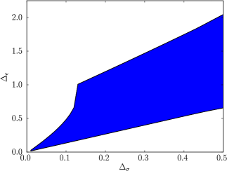
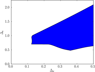
where c𝑐c is the central charge. The power of this infinite-dimensional symmetry was perhaps most famously demonstrated in [1] with the discovery of the minimal models. In addition to providing an exact solution, representation theory of the Virasoro algebra enabled [2, 3, 4, 5] to show that these models are the only unitary CFTs in two dimensions with c<1𝑐1c<1. However, it has become known more recently that one can see hints of the special role played by minimal models without exploiting Virasoro symmetry at all [6, 7, 8, 9, 10, 11, 12, 13]. The method in question is the numerical bootstrap, which uses only the global conformal transformations — two copies of 𝔰𝔩(2)𝔰𝔩2\mathfrak{sl}(2) in this case. Exclusion plots, based on crossing symmetry and unitarity, are shown in Figure 1 where a straight line containing the minimal models is clearly visible.111The algorithm used to generate Figure 1 will become important in section 4. These details are summarized in Appendix B. A kink is present at the Ising point (Δσ,Δϵ)=(18,1)subscriptΔ𝜎subscriptΔitalic-ϵ181(\Delta_{\sigma},\Delta_{\epsilon})=\left(\frac{1}{8},1\right) but, unlike in the three-dimensional case [14, 15, 16], this kink does not sharpen into an island when three correlators are used to restrict the number of relevant operators. Following [17], it is worthwhile to see which features of the 18Δσ1218subscriptΔ𝜎12\frac{1}{8}\leq\Delta_{\sigma}\leq\frac{1}{2} solution can be predicted analytically. The goal of this work is to put the one-correlator upper bound on a more rigorous footing and to explain why the three-correlator upper bound is unchanged.
Refer to caption
(a)
Refer to caption
(b)
Figure 1: Allowed regions for the dimensions of σ𝜎\sigma and ϵitalic-ϵ\epsilon — the 2subscript2\mathbb{Z}_{2}-odd scalar of smallest dimension and the 2subscript2\mathbb{Z}_{2}-even scalar of smallest dimension respectively. The left plot follows from the constraints of crossing symmetry and unitarity on the four-point function σσσσdelimited-⟨⟩𝜎𝜎𝜎𝜎\left<\sigma\sigma\sigma\sigma\right>. The right plot comes from the same constraints on σσσσdelimited-⟨⟩𝜎𝜎𝜎𝜎\left<\sigma\sigma\sigma\sigma\right>, σσϵϵdelimited-⟨⟩𝜎𝜎italic-ϵitalic-ϵ\left<\sigma\sigma\epsilon\epsilon\right> and ϵϵϵϵdelimited-⟨⟩italic-ϵitalic-ϵitalic-ϵitalic-ϵ\left<\epsilon\epsilon\epsilon\epsilon\right>. In both cases, all OPEs are restricted to contain only one relevant scalar.

In order to have a unitary 2D CFT with c<1𝑐1c<1, it is necessary that all primary operators have conformal weights equal to Kac’s formula hr,s(c)subscript𝑟𝑠𝑐h_{r,s}(c) for some (r,s)𝑟𝑠(r,s). The Kac table of degenerate weights is given by

c𝑐\displaystyle c =\displaystyle= 16m(m+1)m>216𝑚𝑚1𝑚2\displaystyle 1-\frac{6}{m(m+1)}\;\;\;\;\;\;\;\;\;\;\;\;\;\;m>2
hr,ssubscript𝑟𝑠\displaystyle h_{r,s} =\displaystyle= [(m+1)rms]214m(m+1)r,s>0.superscriptdelimited-[]𝑚1𝑟𝑚𝑠214𝑚𝑚1𝑟𝑠subscriptabsent0\displaystyle\frac{[(m+1)r-ms]^{2}-1}{4m(m+1)}\;\;\;r,s\in\mathbb{Z}_{>0}\;. (1.2)

Each of these Verma modules has a null state at level rs𝑟𝑠rs. In the operator product expansion (OPE) of primary operators ϕr,ssubscriptitalic-ϕ𝑟𝑠\phi_{r,s} and ϕr,ssubscriptitalic-ϕsuperscript𝑟superscript𝑠\phi_{r^{\prime},s^{\prime}}, the new conformal families that appear are captured in the fusion rule

ϕr,s×ϕr,s=k=0r+r|rr|22l=0s+s|ss|22ϕ|rr|+2k+1,|ss|+2l+1.subscriptitalic-ϕ𝑟𝑠subscriptitalic-ϕsuperscript𝑟superscript𝑠superscriptsubscript𝑘0𝑟superscript𝑟𝑟superscript𝑟22superscriptsubscript𝑙0𝑠superscript𝑠𝑠superscript𝑠22subscriptitalic-ϕ𝑟superscript𝑟2𝑘1𝑠superscript𝑠2𝑙1\phi_{r,s}\times\phi_{r^{\prime},s^{\prime}}=\sum_{k=0}^{\left\lfloor\frac{r+r^{\prime}-|r-r^{\prime}|-2}{2}\right\rfloor}\sum_{l=0}^{\left\lfloor\frac{s+s^{\prime}-|s-s^{\prime}|-2}{2}\right\rfloor}\phi_{|r-r^{\prime}|+2k+1,|s-s^{\prime}|+2l+1}\;. (1.3)

For generic values of m𝑚m, this leads to an infinite discrete spectrum. All OPEs are finite, but as we raise the values of r𝑟r and s𝑠s, these sums become arbitrarily long. A special situation occurs when m𝑚m is an integer. This precisely describes a central charge for which hr,s(c)=hmr,m+1s(c)subscript𝑟𝑠𝑐subscript𝑚𝑟𝑚1𝑠𝑐h_{r,s}(c)=h_{m-r,m+1-s}(c). The Kac table for these doubly degenerate weights can be shown to truncate, allowing us to consider only 0<r<m0𝑟𝑚0<r<m and 0<s<m+10𝑠𝑚10<s<m+1. This leads to a finite number of primary operators and, as it turns out, a unitary theory. This theory, called a (unitary) minimal model, is often denoted (m+1,m)𝑚1𝑚\mathcal{M}(m+1,m). Since Figure 1 only shows a kink for m=3𝑚3m=3, it is evident that non-integer values of m𝑚m are still important for the bootstrap. Analytically continuing the unitary minimal models in this way is not new. In [18, 19], the generic (m+1,m)𝑚1𝑚\mathcal{M}(m+1,m) was found to be a solvable consistent theory and referred to as a generalized minimal model.222This should not be confused with non-unitary minimal model, which describes a non-unitary c<1𝑐1c<1 theory with finitely many primaries. This discrete set is denoted (p,q)𝑝𝑞\mathcal{M}(p,q) with p𝑝p and q𝑞q relatively prime. It obeys the 2D CFT axioms of associativity and Virasoro symmetry but not unitary [20]. The upper bound from the bootstrap

Δϵ=13(8Δσ+2),subscriptΔitalic-ϵ138subscriptΔ𝜎2\Delta_{\epsilon}=\frac{1}{3}(8\Delta_{\sigma}+2)\;, (1.4)

is realized by the generalized minimal model four-point function σσσσdelimited-⟨⟩𝜎𝜎𝜎𝜎\left<\sigma\sigma\sigma\sigma\right> if we identify σϕ1,2𝜎subscriptitalic-ϕ12\sigma\equiv\phi_{1,2} and ϵϕ1,3italic-ϵsubscriptitalic-ϕ13\epsilon\equiv\phi_{1,3}.333This notation differs from the statistical physics literature in which it is natural to regard ϕ2,2subscriptitalic-ϕ22\phi_{2,2} as the spin-field. The authors of [17] observed squared OPE coefficients of quasiprimaries in this correlator that were all positive. If this conjecture is correct, we must conclude that in an arbitrary (m+1,m)𝑚1𝑚\mathcal{M}(m+1,m) theory, the non-unitarity is mild enough that it cannot be diagnosed from the correlator of four σ𝜎\sigma operators. What this means is that for a non-degenerate 𝒪𝒪\mathcal{O} appearing in the σ×σ𝜎𝜎\sigma\times\sigma OPE, the state 𝒪(x1)σ(x2)σ(x3)|0𝒪subscript𝑥1𝜎subscript𝑥2𝜎subscript𝑥3ket0\mathcal{O}(x_{1})\sigma(x_{2})\sigma(x_{3})\left|0\right> on the cylinder will have a positive norm. Similarly, within a degenerate subspace, all such norms will sum to a positive number. We use the terminology that σσσσdelimited-⟨⟩𝜎𝜎𝜎𝜎\left<\sigma\sigma\sigma\sigma\right> comprises a unitary subsector of the theory since other OPEs, e.g. σ×ϵ𝜎italic-ϵ\sigma\times\epsilon, are needed to construct negative norms. As we will show, the conjecture can indeed be proven with the help of a new formalism in [21, 22] for deriving 𝔰𝔩(2)𝔰𝔩2\mathfrak{sl}(2) block expansions. This proof, along with a systematic look at the other two correlators, forms the main result of this work.444Looking ahead, the decompositions (3.21) and (3.26) are essential for the positivity proof. We have learned that they were previously obtained, through a slightly different method, in unpublished work by Mikhail Isachenkov and Volker Schomerus.

Correlator 3<m<43𝑚43<m<4 4<m<4𝑚4<m<\infty
σσσσdelimited-⟨⟩𝜎𝜎𝜎𝜎\left<\sigma\sigma\sigma\sigma\right> All coefficients 0absent0\geq 0 All coefficients 0absent0\geq 0
σσϵϵdelimited-⟨⟩𝜎𝜎italic-ϵitalic-ϵ\left<\sigma\sigma\epsilon\epsilon\right> One checked coefficient <0absent0<0 All checked coefficients 0absent0\geq 0
ϵϵϵϵdelimited-⟨⟩italic-ϵitalic-ϵitalic-ϵitalic-ϵ\left<\epsilon\epsilon\epsilon\epsilon\right> Infinitely many coefficients <0absent0<0 All checked coefficients 0absent0\geq 0
Table 1: The status of three-correlator 𝔰𝔩(2)𝔰𝔩2\mathfrak{sl}(2) block coefficients in the generalized minimal models. Statements about σσσσdelimited-⟨⟩𝜎𝜎𝜎𝜎\left<\sigma\sigma\sigma\sigma\right> apply rigorously to the full set of coefficients. For the other two correlators, we have manually decomposed them up to order 151515.

The summary of results in Table 1 shows that for 3<m<43𝑚43<m<4, σσσσdelimited-⟨⟩𝜎𝜎𝜎𝜎\left<\sigma\sigma\sigma\sigma\right> is the only unitary subsector we have found in the sense described above. However, it appears that the generalized minimal models with m>4𝑚4m>4 have larger unitary subsectors that include the other two four-point functions. The last line shows a surprising tension with Figure 1. Despite the fact that ϵϵϵϵdelimited-⟨⟩italic-ϵitalic-ϵitalic-ϵitalic-ϵ\left<\epsilon\epsilon\epsilon\epsilon\right> displays significant unitarity violation for m<4𝑚4m<4, the line (1.4) in the three-correlator exclusion plot is uninterrupted. The numerics are telling us that there is a partial solution to crossing, other than (m+1,m)𝑚1𝑚\mathcal{M}(m+1,m), which fills in this region. Using the properties of minimal models, we will show that the existence of this solution can be concluded from a simpler numerical setup. It would be nice to eventually find a fully analytic construction.

Before deriving the results in Table 1, it is instructive to consider the lower bound

Δϵ=43Δσ,subscriptΔitalic-ϵ43subscriptΔ𝜎\Delta_{\epsilon}=\frac{4}{3}\Delta_{\sigma}\;, (1.5)

which appears on the left side of Figure 1. This gives us a more straightforward opportunity to use the techniques in [21, 22]. The explicit solution for σσσσdelimited-⟨⟩𝜎𝜎𝜎𝜎\left<\sigma\sigma\sigma\sigma\right> along this line was found in [23], which focused on its special role in the non-unitary (severe truncation) bootstrap of [24, 25, 26].555The fact that it also appears in the unitary bootstrap has not received much attention. In [27], it was mentioned that the lower bound at Δσ=18subscriptΔ𝜎18\Delta_{\sigma}=\frac{1}{8} was somewhat close to Δϵ=16subscriptΔitalic-ϵ16\Delta_{\epsilon}=\frac{1}{6}. Interestingly, the region below the bound coincides with the region where standard OPE maximization techniques cannot constrain the central charge [28]. This solution exhibits Virasoro symmetry with a central charge given by

c=1+16Δσ𝑐116subscriptΔ𝜎c=1+16\Delta_{\sigma} (1.6)

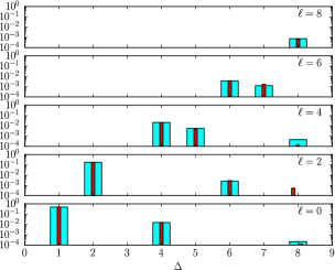
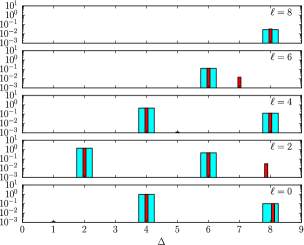
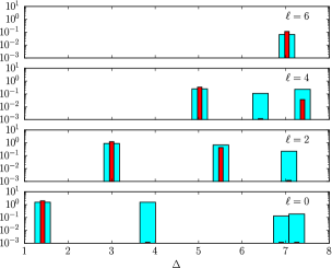
but no Virasoro identity block. To find an analytic explanation for why this four-point function appears in the unitary bootstrap, one must be able to show that this vacuum decoupling is the only sign of non-unitarity that appears at the level of a single correlator. In other words, one must be able to repeat the logic of [17] and find positive squared OPE coefficients for all of the quasiprimaries that do appear. These will be seen as very large coefficients by the numerics because the algorithm used for Figure 1 fixes λσσI=1subscript𝜆𝜎𝜎𝐼1\lambda_{\sigma\sigma I}=1. This is indeed what we find from the extremal functional method of [29].

This paper is organized as follows. In section 2, we study the lower bound (1.5) as a warm-up. In this case, it is particularly easy to invert the OPE and find that all 𝔰𝔩(2)𝔰𝔩2\mathfrak{sl}(2) block coefficients are positive. The methods involved prepare us for our main interest, which is the upper bound (1.4). Turning to this upper bound in section 3, we calculate the global block coefficients summarized in Table 1. In the case of σσσσdelimited-⟨⟩𝜎𝜎𝜎𝜎\left<\sigma\sigma\sigma\sigma\right>, we find closed-form expressions. In showing that they are positive, we prove the conjecture made in the appendix of [17]. For the other two correlators, we expand them to high order recursively and conjecture that the 𝔰𝔩(2)𝔰𝔩2\mathfrak{sl}(2) block coefficients are positive again when 4<m<4𝑚4<m<\infty. Even though the Virasoro blocks in ϵϵϵϵdelimited-⟨⟩italic-ϵitalic-ϵitalic-ϵitalic-ϵ\left<\epsilon\epsilon\epsilon\epsilon\right> appear to have positive 𝔰𝔩(2)𝔰𝔩2\mathfrak{sl}(2) expansions everywhere, the unitarity violation for 3<m<43𝑚43<m<4 arises because of the coefficients multiplying the Virasoro blocks themselves. In section 4, we go back to the bootstrap and discuss what these patterns in the OPE coefficients mean for the results in Figure 1. In particular, we perform a semi-analytic treatment of the problematic correlator. The result is that one does not need to perform a three-correlator bootstrap to predict that (1.4) survives — the search for an upper bound may be reduced to a one-correlator problem. Before concluding, in section 5, we discuss other 2D theories which might be possible to study using more correlators or more assumptions on the spectrum.

2 The lower line: A warm-up

The four-point function along the line (1.5) consists of a single Virasoro block V(hi,h,c;z)𝑉subscript𝑖𝑐𝑧V(h_{i},h,c;z). It was found in [23] via the Coulomb gas formalism which writes the central charge as c=124α02𝑐124superscriptsubscript𝛼02c=1-24\alpha_{0}^{2} and places a background charge of 2α02subscript𝛼02\alpha_{0} at infinity. This allows a number of four-point functions to be realized as correlators of vertex operators with additional insertions of screening charges. The simplest of these is a correlator of four scalars that all have charge α02subscript𝛼02\frac{\alpha_{0}}{2}. Since the neutrality condition for this is satisfied without any screening charges, one finds the manifestly crossing symmetric

σ(0)σ(z,z¯)σ(1)σ()delimited-⟨⟩𝜎0𝜎𝑧¯𝑧𝜎1𝜎\displaystyle\left<\sigma(0)\sigma(z,\bar{z})\sigma(1)\sigma(\infty)\right> =\displaystyle= V(34α02,α02,124α02;z)V(34α02,α02,124α02;z¯)𝑉34superscriptsubscript𝛼02superscriptsubscript𝛼02124superscriptsubscript𝛼02𝑧𝑉34superscriptsubscript𝛼02superscriptsubscript𝛼02124superscriptsubscript𝛼02¯𝑧\displaystyle V\left(-\frac{3}{4}\alpha_{0}^{2},-\alpha_{0}^{2},1-24\alpha_{0}^{2};z\right)V\left(-\frac{3}{4}\alpha_{0}^{2},-\alpha_{0}^{2},1-24\alpha_{0}^{2};\bar{z}\right) (2.1)
=\displaystyle= |z(1z)|α02,superscript𝑧1𝑧superscriptsubscript𝛼02\displaystyle|z(1-z)|^{\alpha_{0}^{2}}\;,

where we have used h=α(α2α0)𝛼𝛼2subscript𝛼0h=\alpha(\alpha-2\alpha_{0}). Expressing (2.1) in terms of ΔσsubscriptΔ𝜎\Delta_{\sigma},

σ(0)σ(z,z¯)σ(1)σ()delimited-⟨⟩𝜎0𝜎𝑧¯𝑧𝜎1𝜎\displaystyle\left<\sigma(0)\sigma(z,\bar{z})\sigma(1)\sigma(\infty)\right> =\displaystyle= g(z)g(z¯)|z|2Δσ𝑔𝑧𝑔¯𝑧superscript𝑧2subscriptΔ𝜎\displaystyle\frac{g(z)g(\bar{z})}{|z|^{2\Delta_{\sigma}}}
g(z)𝑔𝑧\displaystyle g(z) =\displaystyle= z23Δσ(1z)13Δσ.superscript𝑧23subscriptΔ𝜎superscript1𝑧13subscriptΔ𝜎\displaystyle z^{\frac{2}{3}\Delta_{\sigma}}(1-z)^{-\frac{1}{3}\Delta_{\sigma}}\;. (2.2)

Our task now is to expand g(z)𝑔𝑧g(z) into 𝔰𝔩(2)𝔰𝔩2\mathfrak{sl}(2) blocks:

g(z)𝑔𝑧\displaystyle g(z) =\displaystyle= n=0cnK23Δσ+n(z)superscriptsubscript𝑛0subscript𝑐𝑛subscript𝐾23subscriptΔ𝜎𝑛𝑧\displaystyle\sum_{n=0}^{\infty}c_{n}K_{\frac{2}{3}\Delta_{\sigma}+n}(z)
Kh(z)subscript𝐾𝑧\displaystyle K_{h}(z) \displaystyle\equiv zhF12(h,h;2h;z).superscript𝑧subscriptsubscript𝐹122𝑧\displaystyle z^{h}{}_{2}F_{1}(h,h;2h;z)\;. (2.3)

This is guaranteed to be an expansion in even integers due to the Bose symmetry of the σ×σ𝜎𝜎\sigma\times\sigma OPE. To proceed by the brute-force approach, we expand the hypergeometric function and switch the order of two sums.

g(z)𝑔𝑧\displaystyle g(z) =\displaystyle= n=0m=0cn(23Δσ+n)m2(43Δσ+2n)mz23Δσ+n+mm!superscriptsubscript𝑛0superscriptsubscript𝑚0subscript𝑐𝑛superscriptsubscript23subscriptΔ𝜎𝑛𝑚2subscript43subscriptΔ𝜎2𝑛𝑚superscript𝑧23subscriptΔ𝜎𝑛𝑚𝑚\displaystyle\sum_{n=0}^{\infty}\sum_{m=0}^{\infty}c_{n}\frac{\left(\frac{2}{3}\Delta_{\sigma}+n\right)_{m}^{2}}{\left(\frac{4}{3}\Delta_{\sigma}+2n\right)_{m}}\frac{z^{\frac{2}{3}\Delta_{\sigma}+n+m}}{m!} (2.4)
=\displaystyle= k=0n=0kcn(23Δσ+n)kn2(43Δσ+2n)knz23Δσ+k(kn)!superscriptsubscript𝑘0superscriptsubscript𝑛0𝑘subscript𝑐𝑛superscriptsubscript23subscriptΔ𝜎𝑛𝑘𝑛2subscript43subscriptΔ𝜎2𝑛𝑘𝑛superscript𝑧23subscriptΔ𝜎𝑘𝑘𝑛\displaystyle\sum_{k=0}^{\infty}\sum_{n=0}^{k}c_{n}\frac{\left(\frac{2}{3}\Delta_{\sigma}+n\right)_{k-n}^{2}}{\left(\frac{4}{3}\Delta_{\sigma}+2n\right)_{k-n}}\frac{z^{\frac{2}{3}\Delta_{\sigma}+k}}{(k-n)!}

We may now compare the inner finite sums to the Taylor coefficients of (2.2), given by bk=(13Δσ)kk!subscript𝑏𝑘subscript13subscriptΔ𝜎𝑘𝑘b_{k}=\frac{(\frac{1}{3}\Delta_{\sigma})_{k}}{k!}. Since the lower triangular system for cnsubscript𝑐𝑛c_{n} yields to back-substitution,

c2k=b2kn=0k1c2n(23Δσ+2n)2(kn)2(43Δσ+4n)2(kn)1(2k2n)!.subscript𝑐2𝑘subscript𝑏2𝑘superscriptsubscript𝑛0𝑘1subscript𝑐2𝑛superscriptsubscript23subscriptΔ𝜎2𝑛2𝑘𝑛2subscript43subscriptΔ𝜎4𝑛2𝑘𝑛12𝑘2𝑛c_{2k}=b_{2k}-\sum_{n=0}^{k-1}c_{2n}\frac{\left(\frac{2}{3}\Delta_{\sigma}+2n\right)_{2(k-n)}^{2}}{\left(\frac{4}{3}\Delta_{\sigma}+4n\right)_{2(k-n)}}\frac{1}{(2k-2n)!}\;. (2.5)

Rather than using this recursive procedure, we will now review a method for computing the cnsubscript𝑐𝑛c_{n} directly. The blocks, defined in (2.3), are eigenfunctions of the conformal Casimir

DKh(z)𝐷subscript𝐾𝑧\displaystyle DK_{h}(z) =\displaystyle= h(h1)Kh(z)1subscript𝐾𝑧\displaystyle h(h-1)K_{h}(z)
D𝐷\displaystyle D =\displaystyle= z2(1z)2z2z2z.superscript𝑧21𝑧superscript2superscript𝑧2superscript𝑧2𝑧\displaystyle z^{2}(1-z)\frac{\partial^{2}}{\partial z^{2}}-z^{2}\frac{\partial}{\partial z}\;. (2.6)

It is well known that D𝐷D is self-adjoint on [0,1]01[0,1] with respect to the measure z2superscript𝑧2z^{-2}. The authors of [21] used this fact to develop the Sturm-Liouville theory of this operator and construct the orthogonal eigenfunctions

Ψh(z)=Γ(12h)Γ(1h)2Kh(z)+(h1h).\Psi_{h}(z)=\frac{\Gamma(1-2h)}{\Gamma(1-h)^{2}}K_{h}(z)+(h\leftrightarrow 1-h)\;. (2.7)

It is convenient to set h=12+α12𝛼h=\frac{1}{2}+\alpha in which case (2.7) becomes a function Ψα(z)subscriptΨ𝛼𝑧\Psi_{\alpha}(z) which is even in α𝛼\alpha. In order for it to have a finite norm, α𝛼\alpha cannot be real. We must go to imaginary dimension space and take αi𝛼𝑖\alpha\in i\mathbb{R}.666There is another name for this space as evidenced by the title of [21]. The result is that to any four-point function f(z)𝑓𝑧f(z), we may associate a density f^(α)=f^(α)^𝑓𝛼^𝑓𝛼\hat{f}(\alpha)=\hat{f}(-\alpha) via the invertible transform

f(z)𝑓𝑧\displaystyle f(z) =\displaystyle= 12πiiif^(α)Ψα(z)dαN(α)12𝜋𝑖superscriptsubscript𝑖𝑖^𝑓𝛼subscriptΨ𝛼𝑧d𝛼𝑁𝛼\displaystyle\frac{1}{2\pi i}\int_{-i\infty}^{i\infty}\hat{f}(\alpha)\Psi_{\alpha}(z)\frac{\textup{d}\alpha}{N(\alpha)}
N(α)𝑁𝛼\displaystyle N(\alpha) \displaystyle\equiv Γ(α)Γ(α)2πΓ(12+α)Γ(12α).Γ𝛼Γ𝛼2𝜋Γ12𝛼Γ12𝛼\displaystyle\frac{\Gamma(\alpha)\Gamma(-\alpha)}{2\pi\Gamma(\frac{1}{2}+\alpha)\Gamma(\frac{1}{2}-\alpha)}\;. (2.8)

It is now clear that OPE coefficients may be read off from the residues of f^(α)^𝑓𝛼\hat{f}(\alpha) whenever its poles are on the real axis. A formula that [21, 22] derived using this method is

zp(1z)q=n=0(p)n2(2p+n1)nn!F23(n,2p+n1,pqp,p;1)Kp+n(z).superscript𝑧𝑝superscript1𝑧𝑞superscriptsubscript𝑛0superscriptsubscript𝑝𝑛2subscript2𝑝𝑛1𝑛𝑛subscriptsubscript𝐹23fragmentsn,2pn1,pqfragmentsp,p1subscript𝐾𝑝𝑛𝑧z^{p}(1-z)^{-q}=\sum_{n=0}^{\infty}\frac{(p)_{n}^{2}}{(2p+n-1)_{n}n!}{}_{3}F_{2}\left(\begin{tabular}[]{c}$-n,2p+n-1,p-q$\\ $p,p$\end{tabular};1\right)K_{p+n}(z)\;. (2.9)

We will use this in the current section and the next one.

Specializing (2.9) to the four-point function (2.2), we immediately find

cn=(23Δσ)n2(43Δσ+n1)nn!F23(n,43Δσ+n1,13Δσ23Δσ,23Δσ;1).subscript𝑐𝑛superscriptsubscript23subscriptΔ𝜎𝑛2subscript43subscriptΔ𝜎𝑛1𝑛𝑛subscriptsubscript𝐹23fragmentsn,43Δ𝜎n1,13Δ𝜎fragments23Δ𝜎,23Δ𝜎1c_{n}=\frac{\left(\frac{2}{3}\Delta_{\sigma}\right)_{n}^{2}}{\left(\frac{4}{3}\Delta_{\sigma}+n-1\right)_{n}n!}{}_{3}F_{2}\left(\begin{tabular}[]{c}$-n,\frac{4}{3}\Delta_{\sigma}+n-1,\frac{1}{3}\Delta_{\sigma}$\\ $\frac{2}{3}\Delta_{\sigma},\frac{2}{3}\Delta_{\sigma}$\end{tabular};1\right)\;. (2.10)

There are two ways to assess the positivity of (2.10). The first is to recall the definition of a continuous Hahn polynomial [30].

P~n(a,b,c,d;x)=F23(n,n+a+b+c+d1,a+xa+c,a+d;1)subscript~𝑃𝑛𝑎𝑏𝑐𝑑𝑥subscriptsubscript𝐹23fragmentsn,nabcd1,axfragmentsac,ad1\tilde{P}_{n}(a,b,c,d;x)={}_{3}F_{2}\left(\begin{tabular}[]{c}$-n,n+a+b+c+d-1,a+x$\\ $a+c,a+d$\end{tabular};1\right) (2.11)

Clearly,

cn=(23Δσ)n2(43Δσ+n1)nn!P~n(23Δσ,23Δσ,0,0;13Δσ),subscript𝑐𝑛superscriptsubscript23subscriptΔ𝜎𝑛2subscript43subscriptΔ𝜎𝑛1𝑛𝑛subscript~𝑃𝑛23subscriptΔ𝜎23subscriptΔ𝜎0013subscriptΔ𝜎c_{n}=\frac{\left(\frac{2}{3}\Delta_{\sigma}\right)_{n}^{2}}{\left(\frac{4}{3}\Delta_{\sigma}+n-1\right)_{n}n!}\tilde{P}_{n}\left(\frac{2}{3}\Delta_{\sigma},\frac{2}{3}\Delta_{\sigma},0,0;-\frac{1}{3}\Delta_{\sigma}\right)\;, (2.12)

is a valid rewriting of (2.10).777In the notation of [31], we would write cn=2nn!Qn,043Δσ+n(13Δσ)subscript𝑐𝑛superscript2𝑛𝑛superscriptsubscript𝑄𝑛043subscriptΔ𝜎𝑛13subscriptΔ𝜎c_{n}=\frac{2^{-n}}{n!}Q_{n,0}^{\frac{4}{3}\Delta_{\sigma}+n}\left(-\frac{1}{3}\Delta_{\sigma}\right). Suppressing their parameters, the polynomials P~n(a,b,c,d;x)subscript~𝑃𝑛𝑎𝑏𝑐𝑑𝑥\tilde{P}_{n}(a,b,c,d;x) satisfy the following recurrence relation:

(x+a)P~n(x)𝑥𝑎subscript~𝑃𝑛𝑥\displaystyle(x+a)\tilde{P}_{n}(x) =\displaystyle= AnP~n+1(x)(An+Bn)P~n(x)+BnP~n1(x)subscript𝐴𝑛subscript~𝑃𝑛1𝑥subscript𝐴𝑛subscript𝐵𝑛subscript~𝑃𝑛𝑥subscript𝐵𝑛subscript~𝑃𝑛1𝑥\displaystyle A_{n}\tilde{P}_{n+1}(x)-(A_{n}+B_{n})\tilde{P}_{n}(x)+B_{n}\tilde{P}_{n-1}(x)
Ansubscript𝐴𝑛\displaystyle A_{n} \displaystyle\equiv (n+a+b+c+d1)(n+a+c)(n+a+d)(2n+a+b+c+d1)(2n+a+b+c+d)𝑛𝑎𝑏𝑐𝑑1𝑛𝑎𝑐𝑛𝑎𝑑2𝑛𝑎𝑏𝑐𝑑12𝑛𝑎𝑏𝑐𝑑\displaystyle-\frac{(n+a+b+c+d-1)(n+a+c)(n+a+d)}{(2n+a+b+c+d-1)(2n+a+b+c+d)}
Bnsubscript𝐵𝑛\displaystyle B_{n} \displaystyle\equiv n(n+b+c1)(n+b+d1)(2n+a+b+c+d2)(2n+a+b+c+d1).𝑛𝑛𝑏𝑐1𝑛𝑏𝑑12𝑛𝑎𝑏𝑐𝑑22𝑛𝑎𝑏𝑐𝑑1\displaystyle\frac{n(n+b+c-1)(n+b+d-1)}{(2n+a+b+c+d-2)(2n+a+b+c+d-1)}\;. (2.13)

For our parameters, we may easily check that An+Bn+a+x=0subscript𝐴𝑛subscript𝐵𝑛𝑎𝑥0A_{n}+B_{n}+a+x=0. It then follows by induction that all c2k+1subscript𝑐2𝑘1c_{2k+1} vanish. Once we know this, (2.13) is effectively a two-term recursion. Seeing a positive constant of proportionality in

P~2k(13Δσ)subscript~𝑃2𝑘13subscriptΔ𝜎\displaystyle\tilde{P}_{2k}\left(-\frac{1}{3}\Delta_{\sigma}\right) =\displaystyle= B2k1A2k1P~2k2(13Δσ)subscript𝐵2𝑘1subscript𝐴2𝑘1subscript~𝑃2𝑘213subscriptΔ𝜎\displaystyle-\frac{B_{2k-1}}{A_{2k-1}}\tilde{P}_{2k-2}\left(-\frac{1}{3}\Delta_{\sigma}\right) (2.14)
=\displaystyle= 3(2k1)(Δσ+3k3)(2Δσ+3k3)(2Δσ+6k3)P~2k2(13Δσ),32𝑘1subscriptΔ𝜎3𝑘32subscriptΔ𝜎3𝑘32subscriptΔ𝜎6𝑘3subscript~𝑃2𝑘213subscriptΔ𝜎\displaystyle\frac{3(2k-1)(\Delta_{\sigma}+3k-3)}{(2\Delta_{\sigma}+3k-3)(2\Delta_{\sigma}+6k-3)}\tilde{P}_{2k-2}\left(-\frac{1}{3}\Delta_{\sigma}\right)\;,

we conclude that the sequence c2ksubscript𝑐2𝑘c_{2k} decays to zero monotonically from above. It is therefore imperative that the bootstrap single out a region that includes (1.5). To derive this without referring to continuous Hahn polynomials, one may instead express cnsubscript𝑐𝑛c_{n} in terms of gamma functions. This is possible because Watson’s theorem [32],

F23(a,b,ca+b+12,2c;1)=Γ(12)Γ(1+a+b2)Γ(12+c)Γ(1ab2+c)Γ(1+a2)Γ(1+b2)Γ(1a2+c)Γ(1b2+c)subscriptsubscript𝐹23fragmentsa,b,cfragments𝑎𝑏12,2c1Γ12Γ1𝑎𝑏2Γ12𝑐Γ1𝑎𝑏2𝑐Γ1𝑎2Γ1𝑏2Γ1𝑎2𝑐Γ1𝑏2𝑐{}_{3}F_{2}\left(\begin{tabular}[]{c}$a,b,c$\\ $\frac{a+b+1}{2},2c$\end{tabular};1\right)=\frac{\Gamma(\frac{1}{2})\Gamma(\frac{1+a+b}{2})\Gamma(\frac{1}{2}+c)\Gamma(\frac{1-a-b}{2}+c)}{\Gamma(\frac{1+a}{2})\Gamma(\frac{1+b}{2})\Gamma(\frac{1-a}{2}+c)\Gamma(\frac{1-b}{2}+c)} (2.15)

applies whenever p=2q𝑝2𝑞p=2q in (2.9). Although (a+b2c)<1𝑎𝑏2𝑐1\Re(a+b-2c)<1 is usually needed for convergence, we may drop this requirement for a hypergeometric function that terminates.

This analysis does not explain why (1.5) saturates the lower bound in the one-correlator result of Figure 1. However, it is encouraging that bounds of this form in one dimension have been proven in [33]. The Coulomb gas formalism does not yield an obvious way to solve for the correlators σσϵϵdelimited-⟨⟩𝜎𝜎italic-ϵitalic-ϵ\left<\sigma\sigma\epsilon\epsilon\right>, ϵϵϵϵdelimited-⟨⟩italic-ϵitalic-ϵitalic-ϵitalic-ϵ\left<\epsilon\epsilon\epsilon\epsilon\right> or even to verify that they exist. Because the three-correlator plot in Figure 1 excludes this line, any theory to which σσσσdelimited-⟨⟩𝜎𝜎𝜎𝜎\left<\sigma\sigma\sigma\sigma\right> could extend would have to be highly non-unitary.

In this section, we have seen two methods for proving that global block coefficients in (2.2) are positive. One uses Watson’s theorem and the other uses a recurrence relation for orthogonal polynomials. We will need both of these methods when we prove positivity in the generalized minimal models. Before moving on, there is an interesting way to check our results in a spacetime with Minkowski signature. Even though (2.2) is not strictly a correlation function in a unitary theory, it is still bounded in the Regge limit. Its 𝔰𝔩(2)𝔰𝔩2\mathfrak{sl}(2) block expansion should therefore be calculable with the conformal Froissart-Gribov formula [34] which in our case reads

c(Δ,)𝑐Δ\displaystyle c(\Delta,\ell) =\displaystyle= κΔ+0101KΔ+2(z)KΔ+22(z¯)dDisc[|z|2Δσσ(0)σ(z,z¯)σ(1)σ()]dzz2dz¯z¯2subscript𝜅Δsuperscriptsubscript01superscriptsubscript01subscript𝐾Δ2𝑧subscript𝐾Δ22¯𝑧dDiscdelimited-[]superscript𝑧2subscriptΔ𝜎delimited-⟨⟩𝜎0𝜎𝑧¯𝑧𝜎1𝜎d𝑧superscript𝑧2d¯𝑧superscript¯𝑧2\displaystyle\kappa_{\Delta+\ell}\int_{0}^{1}\int_{0}^{1}K_{\frac{\Delta+\ell}{2}}(z)K_{\frac{\ell-\Delta+2}{2}}(\bar{z})\mathrm{dDisc}[|z|^{2\Delta_{\sigma}}\left<\sigma(0)\sigma(z,\bar{z})\sigma(1)\sigma(\infty)\right>]\frac{\textup{d}z}{z^{2}}\frac{\textup{d}\bar{z}}{\bar{z}^{2}}
κβsubscript𝜅𝛽\displaystyle\kappa_{\beta} \displaystyle\equiv Γ(β2)42π2Γ(β1)Γ(β).Γsuperscript𝛽242superscript𝜋2Γ𝛽1Γ𝛽\displaystyle\frac{\Gamma(\frac{\beta}{2})^{4}}{2\pi^{2}\Gamma(\beta-1)\Gamma(\beta)}\;. (2.16)

To define the double-discontinuity, we must treat z,z¯𝑧¯𝑧z,\bar{z} as independent variables and rotate around the z¯=1¯𝑧1\bar{z}=1 branch point. Since this can be done in two ways, we subtract the average from our four-point function to find

dDisc[g(z)g(z¯)]=2sin2(πΔσ3)(zz¯)23Δσ[(1z)(1z¯)]13Δσ.dDiscdelimited-[]𝑔𝑧𝑔¯𝑧2superscript2𝜋subscriptΔ𝜎3superscript𝑧¯𝑧23subscriptΔ𝜎superscriptdelimited-[]1𝑧1¯𝑧13subscriptΔ𝜎\mathrm{dDisc}\left[g(z)g(\bar{z})\right]=2\sin^{2}\left(\frac{\pi\Delta_{\sigma}}{3}\right)(z\bar{z})^{\frac{2}{3}\Delta_{\sigma}}[(1-z)(1-\bar{z})]^{-\frac{1}{3}\Delta_{\sigma}}\;. (2.17)

Performing the factored integrals yields a spectral density given by

c(Δ,)Γ(113Δσ)22sin2(πΔσ3)κΔ+𝑐ΔΓsuperscript113subscriptΔ𝜎22superscript2𝜋subscriptΔ𝜎3subscript𝜅Δ\displaystyle\frac{c(\Delta,\ell)\Gamma(1-\frac{1}{3}\Delta_{\sigma})^{-2}}{2\sin^{2}\left(\frac{\pi\Delta_{\sigma}}{3}\right)\kappa_{\Delta+\ell}} =\displaystyle= Γ(23Δσ+Δ2)Γ(13Δσ+Δ+22)F23(Δ+22,Δ+22,23Δσ+Δ2Δ+2,13Δσ+Δ+22;1)Γ23subscriptΔ𝜎Δ2Γ13subscriptΔ𝜎Δ22subscriptsubscript𝐹23fragmentsΔ22,Δ22,23Δ𝜎Δ2fragmentsΔ2,13Δ𝜎Δ221\displaystyle\frac{\Gamma(\frac{2}{3}\Delta_{\sigma}+\frac{\ell-\Delta}{2})}{\Gamma(\frac{1}{3}\Delta_{\sigma}+\frac{\ell-\Delta+2}{2})}{}_{3}F_{2}\left(\begin{tabular}[]{c}$\frac{\ell-\Delta+2}{2},\frac{\ell-\Delta+2}{2},\frac{2}{3}\Delta_{\sigma}+\frac{\ell-\Delta}{2}$\\ $\ell-\Delta+2,\frac{1}{3}\Delta_{\sigma}+\frac{\ell-\Delta+2}{2}$\end{tabular};1\right) (2.23)
Γ(23Δσ+Δ+22)Γ(13Δσ+Δ+2)F23(Δ+2,Δ+2,23Δσ+Δ+22Δ+,13Δσ+Δ+2;1)Γ23subscriptΔ𝜎Δ22Γ13subscriptΔ𝜎Δ2subscriptsubscript𝐹23fragmentsΔ2,Δ2,23Δ𝜎Δ22fragmentsΔ,13Δ𝜎Δ21\displaystyle\frac{\Gamma(\frac{2}{3}\Delta_{\sigma}+\frac{\Delta+\ell-2}{2})}{\Gamma(\frac{1}{3}\Delta_{\sigma}+\frac{\Delta+\ell}{2})}{}_{3}F_{2}\left(\begin{tabular}[]{c}$\frac{\Delta+\ell}{2},\frac{\Delta+\ell}{2},\frac{2}{3}\Delta_{\sigma}+\frac{\Delta+\ell-2}{2}$\\ $\Delta+\ell,\frac{1}{3}\Delta_{\sigma}+\frac{\Delta+\ell}{2}$\end{tabular};1\right)

with poles at Δ=43Δσ+2nΔ43subscriptΔ𝜎2𝑛\Delta-\ell=\frac{4}{3}\Delta_{\sigma}+2n. As none of these are integers, the correct prescription for finding OPE coefficients is to simply take the residue [34].

Res(c(Δ,),n)Res𝑐Δ𝑛\displaystyle-\mathrm{Res}\left(c(\Delta,\ell),n\right) =\displaystyle= (1)nn!8sin2(πΔσ3)κ43Δσ+2+2nΓ(113Δσ)2Γ(43Δσ+n+1)Γ(Δσ++n)Γ(113Δσn)superscript1𝑛𝑛8superscript2𝜋subscriptΔ𝜎3subscript𝜅43subscriptΔ𝜎22𝑛Γsuperscript113subscriptΔ𝜎2Γ43subscriptΔ𝜎𝑛1ΓsubscriptΔ𝜎𝑛Γ113subscriptΔ𝜎𝑛\displaystyle\frac{(-1)^{n}}{n!}\frac{8\sin^{2}\left(\frac{\pi\Delta_{\sigma}}{3}\right)\kappa_{\frac{4}{3}\Delta_{\sigma}+2\ell+2n}\Gamma(1-\frac{1}{3}\Delta_{\sigma})^{2}\Gamma(\frac{4}{3}\Delta_{\sigma}+n+\ell-1)}{\Gamma(\Delta_{\sigma}+\ell+n)\Gamma(1-\frac{1}{3}\Delta_{\sigma}-n)} (2.29)
F23(43Δσ++n1,23Δσ++n,23Δσ++nΔσ++n,43Δσ+2+2n;1)subscriptsubscript𝐹23fragments43Δ𝜎n1,23Δ𝜎n,23Δ𝜎nfragmentsΔ𝜎n,43Δ𝜎22n1\displaystyle{}_{3}F_{2}\left(\begin{tabular}[]{c}$\frac{4}{3}\Delta_{\sigma}+\ell+n-1,\frac{2}{3}\Delta_{\sigma}+\ell+n,\frac{2}{3}\Delta_{\sigma}+\ell+n$\\ $\Delta_{\sigma}+\ell+n,\frac{4}{3}\Delta_{\sigma}+2\ell+2n$\end{tabular};1\right)
F23(n,1n23Δσ,1n23Δσ1n13Δσ,22n43Δσ;1)subscriptsubscript𝐹23fragmentsn,1n23Δ𝜎,1n23Δ𝜎fragments1n13Δ𝜎,22n43Δ𝜎1\displaystyle{}_{3}F_{2}\left(\begin{tabular}[]{c}$-n,1-n-\frac{2}{3}\Delta_{\sigma},1-n-\frac{2}{3}\Delta_{\sigma}$\\ $1-n-\frac{1}{3}\Delta_{\sigma},2-2n-\frac{4}{3}\Delta_{\sigma}$\end{tabular};1\right)

Although it is not obvious, we have checked that (2.29) is equal to cncn+subscript𝑐𝑛subscript𝑐𝑛c_{n}c_{n+\ell} by using Watson’s theorem twice.

3 The upper line: One and three correlators

Each state |hr,sketsubscript𝑟𝑠\left|h_{r,s}\right> dual to a degenerate operator in a generalized minimal model has a null descendant |χr,sketsubscript𝜒𝑟𝑠\left|\chi_{r,s}\right> at level rs𝑟𝑠rs called a singular vector. Four-point functions may be calculated once the necessary singular vectors are known. We simply convert χr,ssubscript𝜒𝑟𝑠\chi_{r,s} to a differential operator with the Ward identities

Lnnmaps-tosubscript𝐿𝑛subscript𝑛\displaystyle L_{-n}\mapsto\mathcal{L}_{-n} =\displaystyle= i1hi(n1)(ziz1)ni(ziz1)n1subscript𝑖1subscript𝑖𝑛1superscriptsubscript𝑧𝑖subscript𝑧1𝑛subscript𝑖superscriptsubscript𝑧𝑖subscript𝑧1𝑛1\displaystyle\sum_{i\neq 1}\frac{h_{i}(n-1)}{(z_{i}-z_{1})^{n}}-\frac{\partial_{i}}{(z_{i}-z_{1})^{n-1}}
L11maps-tosubscript𝐿1subscript1\displaystyle L_{-1}\mapsto\mathcal{L}_{-1} =\displaystyle= 1,subscript1\displaystyle\partial_{1}\;, (3.1)

and use the fact that this operator must annihilate any correlation function involving ϕr,ssubscriptitalic-ϕ𝑟𝑠\phi_{r,s} in the first position. The resulting equation, known as a BPZ differential equation [1], has rs𝑟𝑠rs linearly independent solutions representing the exchanged multiplets. One may read off their dimensions by looking at the O(zh)𝑂superscript𝑧O(z^{h}) behaviour as z0𝑧0z\rightarrow 0. While expressions for singular vectors are generally non-trivial, with some appearing only recently [35, 36, 37], the ones we need are relatively simple:

|χ1,sketsubscript𝜒1𝑠\displaystyle\left|\chi_{1,s}\right> =\displaystyle= p1++pk=s(t)sk[(s1)!]2i=1k1(p1++pi)(sp1pi)Lp1Lpk|h1,ssubscriptsubscript𝑝1subscript𝑝𝑘𝑠superscript𝑡𝑠𝑘superscriptdelimited-[]𝑠12superscriptsubscriptproduct𝑖1𝑘1subscript𝑝1subscript𝑝𝑖𝑠subscript𝑝1subscript𝑝𝑖subscript𝐿𝑝1subscript𝐿subscript𝑝𝑘ketsubscript1𝑠\displaystyle\sum_{p_{1}+\dots+p_{k}=s}\frac{(-t)^{s-k}[(s-1)!]^{2}}{\prod_{i=1}^{k-1}(p_{1}+\dots+p_{i})(s-p_{1}-\dots-p_{i})}L_{-p1}\dots L_{-p_{k}}\left|h_{1,s}\right>
t𝑡\displaystyle t \displaystyle\equiv mm+1.𝑚𝑚1\displaystyle\frac{m}{m+1}\;. (3.2)
Fusion rules Weights
ϕ1,2×ϕ1,2=ϕ1,1+ϕ1,3subscriptitalic-ϕ12subscriptitalic-ϕ12subscriptitalic-ϕ11subscriptitalic-ϕ13\phi_{1,2}\times\phi_{1,2}=\phi_{1,1}+\phi_{1,3} h1,1=0subscript110h_{1,1}=0
ϕ1,2×ϕ1,3=ϕ1,2+ϕ1,4subscriptitalic-ϕ12subscriptitalic-ϕ13subscriptitalic-ϕ12subscriptitalic-ϕ14\phi_{1,2}\times\phi_{1,3}=\phi_{1,2}+\phi_{1,4} h1,2=Δσ2subscript12subscriptΔ𝜎2h_{1,2}=\frac{\Delta_{\sigma}}{2}
ϕ1,3×ϕ1,3=ϕ1,1+ϕ1,3+ϕ1,5subscriptitalic-ϕ13subscriptitalic-ϕ13subscriptitalic-ϕ11subscriptitalic-ϕ13subscriptitalic-ϕ15\phi_{1,3}\times\phi_{1,3}=\phi_{1,1}+\phi_{1,3}+\phi_{1,5} h1,3=4Δσ+13Δϵ2subscript134subscriptΔ𝜎13subscriptΔitalic-ϵ2h_{1,3}=\frac{4\Delta_{\sigma}+1}{3}\equiv\frac{\Delta_{\epsilon}}{2}
h1,4=5Δσ+22subscript145subscriptΔ𝜎22h_{1,4}=\frac{5\Delta_{\sigma}+2}{2}
h1,5=4Δσ+2subscript154subscriptΔ𝜎2h_{1,5}=4\Delta_{\sigma}+2
Table 2: Operators that can appear in σσσσdelimited-⟨⟩𝜎𝜎𝜎𝜎\left<\sigma\sigma\sigma\sigma\right>, σσϵϵdelimited-⟨⟩𝜎𝜎italic-ϵitalic-ϵ\left<\sigma\sigma\epsilon\epsilon\right>, ϵϵϵϵdelimited-⟨⟩italic-ϵitalic-ϵitalic-ϵitalic-ϵ\left<\epsilon\epsilon\epsilon\epsilon\right> and their holomorphic weights. The fusion rules would shorten e.g. in the Ising model m=3𝑚3m=3 and tricritical Ising model m=4𝑚4m=4, but we are interested in (m+1,m)𝑚1𝑚\mathcal{M}(m+1,m) for real m𝑚m.

It is clear that we may confine ourselves to the border of the Kac table when studying correlators of σϕ1,2𝜎subscriptitalic-ϕ12\sigma\equiv\phi_{1,2} and ϵϕ1,3italic-ϵsubscriptitalic-ϕ13\epsilon\equiv\phi_{1,3}. The set of operators ϕ1,ssubscriptitalic-ϕ1𝑠\phi_{1,s} which closes under fusion is called the Verlinde subalgebra. We will continue to parametrize the generalized minimal model by ΔσsubscriptΔ𝜎\Delta_{\sigma} — the horizontal axis of Figure 1. For convenience, Table 2 summarizes the OPEs that are important for the simplest mixed correlator system.

3.1 All global block coefficients in the simplest correlator

We will now derive new expressions for the squared OPE coefficients in σσσσdelimited-⟨⟩𝜎𝜎𝜎𝜎\left<\sigma\sigma\sigma\sigma\right> along (1.4). Positivity, as predicted by [17], will then follow from methods analogous to those in the last section. Since this correlator solves a second-order BPZ equation, we may write it as

σ(z1,z¯1)σ(z2,z¯2)σ(z3,z¯3)σ(z4,z¯4)=G(z,z¯)|z12z34|2Δσdelimited-⟨⟩𝜎subscript𝑧1subscript¯𝑧1𝜎subscript𝑧2subscript¯𝑧2𝜎subscript𝑧3subscript¯𝑧3𝜎subscript𝑧4subscript¯𝑧4𝐺𝑧¯𝑧superscriptsubscript𝑧12subscript𝑧342subscriptΔ𝜎\displaystyle\left<\sigma(z_{1},\bar{z}_{1})\sigma(z_{2},\bar{z}_{2})\sigma(z_{3},\bar{z}_{3})\sigma(z_{4},\bar{z}_{4})\right>=\frac{G(z,\bar{z})}{|z_{12}z_{34}|^{2\Delta_{\sigma}}}
G(z,z¯)=G(1,1)σσσσ(z)G(1,1)σσσσ(z¯)+C(1,2)(1,2)(1,3)G(1,3)σσσσ(z)G(1,3)σσσσ(z¯),𝐺𝑧¯𝑧subscriptsuperscript𝐺𝜎𝜎𝜎𝜎11𝑧subscriptsuperscript𝐺𝜎𝜎𝜎𝜎11¯𝑧subscriptsuperscript𝐶131212subscriptsuperscript𝐺𝜎𝜎𝜎𝜎13𝑧subscriptsuperscript𝐺𝜎𝜎𝜎𝜎13¯𝑧\displaystyle G(z,\bar{z})=G^{\sigma\sigma\sigma\sigma}_{(1,1)}(z)G^{\sigma\sigma\sigma\sigma}_{(1,1)}(\bar{z})+C^{(1,3)}_{(1,2)(1,2)}G^{\sigma\sigma\sigma\sigma}_{(1,3)}(z)G^{\sigma\sigma\sigma\sigma}_{(1,3)}(\bar{z})\;, (3.3)

where the functions of z𝑧z are Virasoro blocks.888For the moment, we will be concerned with the global OPE coefficients contained within each one. The overall coefficients C(r1,s1)(r2,s2)(r3,s3)superscriptsubscript𝐶subscript𝑟1subscript𝑠1subscript𝑟2subscript𝑠2subscript𝑟3subscript𝑠3C_{(r_{1},s_{1})(r_{2},s_{2})}^{(r_{3},s_{3})} are the generalized minimal model structure constants that were obtained with the Coulomb gas formalism in [38, 39, 40]. The specific operator, read off from (3.2), is

32(Δσ+1)122.32subscriptΔ𝜎1superscriptsubscript12subscript2\frac{3}{2(\Delta_{\sigma}+1)}\mathcal{L}_{-1}^{2}-\mathcal{L}_{-2}\;. (3.4)

Acting on (3.3) with (3.4), we arrive at a PDE in terms of (z1,z2,z3,z4)subscript𝑧1subscript𝑧2subscript𝑧3subscript𝑧4(z_{1},z_{2},z_{3},z_{4}). To reduce it to an ODE, we map these points to (0,z,1,)0𝑧1(0,z,1,\infty) by a global conformal transformation:

32z(z1)22Gz2+(z1)[(2Δσ)z+2Δσ1]Gz12Δσ(Δσ+1)zG=0.32𝑧superscript𝑧12superscript2𝐺superscript𝑧2𝑧1delimited-[]2subscriptΔ𝜎𝑧2subscriptΔ𝜎1𝐺𝑧12subscriptΔ𝜎subscriptΔ𝜎1𝑧𝐺0\frac{3}{2}z(z-1)^{2}\frac{\partial^{2}G}{\partial z^{2}}+(z-1)[(2-\Delta_{\sigma})z+2\Delta_{\sigma}-1]\frac{\partial G}{\partial z}-\frac{1}{2}\Delta_{\sigma}(\Delta_{\sigma}+1)zG=0\;. (3.5)

Well known solutions, which have the expected asymptotic behaviour, are

G(1,1)σσσσ(z)subscriptsuperscript𝐺𝜎𝜎𝜎𝜎11𝑧\displaystyle G^{\sigma\sigma\sigma\sigma}_{(1,1)}(z) =\displaystyle= (1z)ΔσF12(2Δσ,12Δσ3;24Δσ3;z)superscript1𝑧subscriptΔ𝜎subscriptsubscript𝐹122subscriptΔ𝜎12subscriptΔ𝜎324subscriptΔ𝜎3𝑧\displaystyle(1-z)^{-\Delta_{\sigma}}{}_{2}F_{1}\left(-2\Delta_{\sigma},\frac{1-2\Delta_{\sigma}}{3};\frac{2-4\Delta_{\sigma}}{3};z\right)
G(1,3)σσσσ(z)subscriptsuperscript𝐺𝜎𝜎𝜎𝜎13𝑧\displaystyle G^{\sigma\sigma\sigma\sigma}_{(1,3)}(z) =\displaystyle= z1+4Δσ3(1z)ΔσF12(12Δσ3,2+2Δσ3;4+4Δσ3;z).superscript𝑧14subscriptΔ𝜎3superscript1𝑧subscriptΔ𝜎subscriptsubscript𝐹1212subscriptΔ𝜎322subscriptΔ𝜎344subscriptΔ𝜎3𝑧\displaystyle z^{\frac{1+4\Delta_{\sigma}}{3}}(1-z)^{-\Delta_{\sigma}}{}_{2}F_{1}\left(\frac{1-2\Delta_{\sigma}}{3},\frac{2+2\Delta_{\sigma}}{3};\frac{4+4\Delta_{\sigma}}{3};z\right)\;. (3.6)

First, let us look at the identity block. After a quadratic transformation, the hypergeometric function becomes a series in z24z4superscript𝑧24𝑧4\frac{z^{2}}{4z-4}. This makes the formula (2.9) applicable if we set p=2n𝑝2𝑛p=2n and q=n𝑞𝑛q=n.

G(1,1)σσσσ(z)=F12(Δσ,1+Δσ3;54Δσ6;14z2z1)subscriptsuperscript𝐺𝜎𝜎𝜎𝜎11𝑧subscriptsubscript𝐹12subscriptΔ𝜎1subscriptΔ𝜎354subscriptΔ𝜎614superscript𝑧2𝑧1\displaystyle G^{\sigma\sigma\sigma\sigma}_{(1,1)}(z)={}_{2}F_{1}\left(-\Delta_{\sigma},\frac{1+\Delta_{\sigma}}{3};\frac{5-4\Delta_{\sigma}}{6};\frac{1}{4}\frac{z^{2}}{z-1}\right) (3.7)
=n=0(14)n(Δσ)n(1+Δσ3)n(54Δσ6)nn!m=0(2n)m2(4n+m1)mm!F23(m,4n+m1,n2n,2n;1)K2n+m(z)absentsuperscriptsubscript𝑛0superscript14𝑛subscriptsubscriptΔ𝜎𝑛subscript1subscriptΔ𝜎3𝑛subscript54subscriptΔ𝜎6𝑛𝑛superscriptsubscript𝑚0superscriptsubscript2𝑛𝑚2subscript4𝑛𝑚1𝑚𝑚subscriptsubscript𝐹23fragmentsm,4nm1,nfragments2n,2n1subscript𝐾2𝑛𝑚𝑧\displaystyle=\sum_{n=0}^{\infty}\left(-\frac{1}{4}\right)^{n}\frac{(-\Delta_{\sigma})_{n}\left(\frac{1+\Delta_{\sigma}}{3}\right)_{n}}{\left(\frac{5-4\Delta_{\sigma}}{6}\right)_{n}n!}\sum_{m=0}^{\infty}\frac{(2n)_{m}^{2}}{(4n+m-1)_{m}m!}{}_{3}F_{2}\left(\begin{tabular}[]{c}$-m,4n+m-1,n$\\ $2n,2n$\end{tabular};1\right)K_{2n+m}(z) (3.10)

Exchanging the two sums, we find

c2k=n=0k(14)n(Δσ)n(1+Δσ3)n(54Δσ6)nn!(2n)2k2n2(2n+2k1)2k2n(2k2n)!F23(2n2k,2n+2k1,n2n,2n;1)subscript𝑐2𝑘superscriptsubscript𝑛0𝑘superscript14𝑛subscriptsubscriptΔ𝜎𝑛subscript1subscriptΔ𝜎3𝑛subscript54subscriptΔ𝜎6𝑛𝑛subscriptsuperscript2𝑛22𝑘2𝑛subscript2𝑛2𝑘12𝑘2𝑛2𝑘2𝑛subscriptsubscript𝐹23fragments2n2k,2n2k1,nfragments2n,2n1c_{2k}=\sum_{n=0}^{k}\left(-\frac{1}{4}\right)^{n}\frac{(-\Delta_{\sigma})_{n}\left(\frac{1+\Delta_{\sigma}}{3}\right)_{n}}{\left(\frac{5-4\Delta_{\sigma}}{6}\right)_{n}n!}\frac{(2n)^{2}_{2k-2n}}{(2n+2k-1)_{2k-2n}(2k-2n)!}{}_{3}F_{2}\left(\begin{tabular}[]{c}$2n-2k,2n+2k-1,n$\\ $2n,2n$\end{tabular};1\right) (3.11)

for the non-vanishing global block coefficients.999We derived this by applying a quadratic transformation to (3.6) which makes the Bose symmetry manifest. By leaving the function in its original form, or by applying Euler / Pfaff transformations, we can derive other sums that are non-trivially equivalent to (3.11). Since p=2q𝑝2𝑞p=2q, this hypergeometric is in a form that can be treated with Watson’s theorem. When we apply this to the c2ksubscript𝑐2𝑘c_{2k}, one pole in the numerator cancels another in the denominator.101010Because we have not allowed for other poles, our expression for c2ksubscript𝑐2𝑘c_{2k} will not be correct for k=0𝑘0k=0. There is no need to treat this case separately as it is already clear that c0=1subscript𝑐01c_{0}=1.

F23(2n2k,2n+2k1,n2n,2n;1)subscriptsubscript𝐹23fragments2n2k,2n2k1,nfragments2n,2n1\displaystyle{}_{3}F_{2}\left(\begin{tabular}[]{c}$2n-2k,2n+2k-1,n$\\ $2n,2n$\end{tabular};1\right) =\displaystyle= (1)n+kΓ(12)Γ(n+12)Γ(2n)Γ(n)Γ(nk+12)Γ(2n+2k1)(k1)!(n1)!superscript1𝑛𝑘Γ12Γ𝑛12Γ2𝑛Γ𝑛Γ𝑛𝑘12Γ2𝑛2𝑘1𝑘1𝑛1\displaystyle\frac{(-1)^{n+k}\Gamma(\frac{1}{2})\Gamma(n+\frac{1}{2})\Gamma(2n)}{\Gamma(n)\Gamma(n-k+\frac{1}{2})\Gamma(2n+2k-1)}\frac{(k-1)!}{(n-1)!}
=\displaystyle= (1)n+kΓ(2n)2Γ(2n+2k1)Γ(n+k12)Γ(12)Γ(nk+12)Γ(k+12)limδ022k1(k1)![Γ(δ)(δ)n]2superscript1𝑛𝑘Γsuperscript2𝑛2Γ2𝑛2𝑘1Γ𝑛𝑘12Γ12Γ𝑛𝑘12Γ𝑘12subscript𝛿0superscript22𝑘1𝑘1superscriptdelimited-[]Γ𝛿subscript𝛿𝑛2\displaystyle\frac{(-1)^{n+k}\Gamma(2n)^{2}}{\Gamma(2n+2k-1)}\frac{\Gamma(n+k-\frac{1}{2})\Gamma(\frac{1}{2})}{\Gamma(n-k+\frac{1}{2})\Gamma(k+\frac{1}{2})}\lim_{\delta\rightarrow 0}\frac{2^{2k-1}(k-1)!}{[\Gamma(\delta)(\delta)_{n}]^{2}}

Above, we can easily see three gamma functions that will cancel when we multiply by (2n)2k2n2(2n+2k1)2k2n(2k2n)!subscriptsuperscript2𝑛22𝑘2𝑛subscript2𝑛2𝑘12𝑘2𝑛2𝑘2𝑛\frac{(2n)^{2}_{2k-2n}}{(2n+2k-1)_{2k-2n}(2k-2n)!}. We have also written 1Γ(n)21Γsuperscript𝑛2\frac{1}{\Gamma(n)^{2}} in a limiting form for later convenience. After substituting (3.1), one must use the identities

Γ(x+n)=Γ(x)(x)n,Γ(xn)=(1)nΓ(x)(1x)nformulae-sequenceΓ𝑥𝑛Γ𝑥subscript𝑥𝑛Γ𝑥𝑛superscript1𝑛Γ𝑥subscript1𝑥𝑛\Gamma(x+n)=\Gamma(x)(x)_{n}\;\;\;,\;\;\;\Gamma(x-n)=(-1)^{n}\frac{\Gamma(x)}{(1-x)_{n}} (3.15)

until each term of (3.11) only depends on n𝑛n through the Pochhammer symbol. This leads to

c2ksubscript𝑐2𝑘\displaystyle c_{2k} =\displaystyle= (4k22k1)1limδ01k(2k1)Γ(δ)2F34(k,k12,Δσ,1+Δσ3δ,δ,54Δσ6;1)superscriptbinomial4𝑘22𝑘11subscript𝛿01𝑘2𝑘1Γsuperscript𝛿2subscriptsubscript𝐹34fragmentsk,k12,Δ𝜎,1subscriptΔ𝜎3fragmentsδ,δ,54subscriptΔ𝜎61\displaystyle\binom{4k-2}{2k-1}^{-1}\lim_{\delta\rightarrow 0}\frac{1}{k(2k-1)\Gamma(\delta)^{2}}{}_{4}F_{3}\left(\begin{tabular}[]{c}$-k,k-\frac{1}{2},-\Delta_{\sigma},\frac{1+\Delta_{\sigma}}{3}$\\ $\delta,\delta,\frac{5-4\Delta_{\sigma}}{6}$\end{tabular};1\right) (3.18)
=\displaystyle= (4k22k1)1Δσ(1+Δσ)54ΔσF34(1k,k+12,1Δσ,4+Δσ31,2,114Δσ6;1).superscriptbinomial4𝑘22𝑘11subscriptΔ𝜎1subscriptΔ𝜎54subscriptΔ𝜎subscriptsubscript𝐹34fragments1k,k12,1Δ𝜎,4subscriptΔ𝜎3fragments1,2,114subscriptΔ𝜎61\displaystyle\binom{4k-2}{2k-1}^{-1}\frac{\Delta_{\sigma}(1+\Delta_{\sigma})}{5-4\Delta_{\sigma}}{}_{4}F_{3}\left(\begin{tabular}[]{c}$1-k,k+\frac{1}{2},1-\Delta_{\sigma},\frac{4+\Delta_{\sigma}}{3}$\\ $1,2,\frac{11-4\Delta_{\sigma}}{6}$\end{tabular};1\right)\;. (3.21)

The ϵitalic-ϵ\epsilon block can be analyzed in the same way. Doing so will in fact be easier since we will not have to pass to the δ0𝛿0\delta\rightarrow 0 limit. Starting from

G(1,3)σσσσ(z)=z1+4Δσ3(1z)1+4Δσ6F12(1+2Δσ2,12Δσ6;7+4Δσ6;14z2z1),subscriptsuperscript𝐺𝜎𝜎𝜎𝜎13𝑧superscript𝑧14subscriptΔ𝜎3superscript1𝑧14subscriptΔ𝜎6subscriptsubscript𝐹1212subscriptΔ𝜎212subscriptΔ𝜎674subscriptΔ𝜎614superscript𝑧2𝑧1G^{\sigma\sigma\sigma\sigma}_{(1,3)}(z)=z^{\frac{1+4\Delta_{\sigma}}{3}}(1-z)^{-\frac{1+4\Delta_{\sigma}}{6}}{}_{2}F_{1}\left(\frac{1+2\Delta_{\sigma}}{2},\frac{1-2\Delta_{\sigma}}{6};\frac{7+4\Delta_{\sigma}}{6};\frac{1}{4}\frac{z^{2}}{z-1}\right)\;, (3.22)

we may use (2.9) with p=1+4Δσ3+2n𝑝14subscriptΔ𝜎32𝑛p=\frac{1+4\Delta_{\sigma}}{3}+2n and q=1+4Δσ6+n𝑞14subscriptΔ𝜎6𝑛q=\frac{1+4\Delta_{\sigma}}{6}+n. This leads to

c2ksubscript𝑐2𝑘\displaystyle c_{2k} =\displaystyle= n=0k(14)n(1+2Δσ6)n(1+2Δσ2)n(7+4Δσ6)nn!(1+4Δσ3+2n)2k2n2(2+8Δσ3+2n+2k1)2k2n(2k2n)!superscriptsubscript𝑛0𝑘superscript14𝑛subscript12subscriptΔ𝜎6𝑛subscript12subscriptΔ𝜎2𝑛subscript74subscriptΔ𝜎6𝑛𝑛subscriptsuperscript14subscriptΔ𝜎32𝑛22𝑘2𝑛subscript28subscriptΔ𝜎32𝑛2𝑘12𝑘2𝑛2𝑘2𝑛\displaystyle\sum_{n=0}^{k}\left(-\frac{1}{4}\right)^{n}\frac{\left(\frac{1+2\Delta_{\sigma}}{6}\right)_{n}\left(\frac{1+2\Delta_{\sigma}}{2}\right)_{n}}{\left(\frac{7+4\Delta_{\sigma}}{6}\right)_{n}n!}\frac{\left(\frac{1+4\Delta_{\sigma}}{3}+2n\right)^{2}_{2k-2n}}{\left(\frac{2+8\Delta_{\sigma}}{3}+2n+2k-1\right)_{2k-2n}(2k-2n)!} (3.25)
F23(2n2k,2+8Δσ3+2n+2k1,1+4Δσ6+n1+4Δσ3+2n,1+4Δσ3+2n;1)subscriptsubscript𝐹23fragments2n2k,28subscriptΔ𝜎32n2k1,14subscriptΔ𝜎6nfragments14subscriptΔ𝜎32n,14subscriptΔ𝜎32n1\displaystyle{}_{3}F_{2}\left(\begin{tabular}[]{c}$2n-2k,\frac{2+8\Delta_{\sigma}}{3}+2n+2k-1,\frac{1+4\Delta_{\sigma}}{6}+n$\\ $\frac{1+4\Delta_{\sigma}}{3}+2n,\frac{1+4\Delta_{\sigma}}{3}+2n$\end{tabular};1\right)

which again allows us to use Watson’s theorem. Employing (3.15) to perform the sum, we arrive at

c2k=14kk!(1+4Δσ6)k2(1+4Δσ3+k12)kF34(k,1+4Δσ3+k12,Δσ+12,12Δσ61+4Δσ6,1+4Δσ6,7+4Δσ6;1).subscript𝑐2𝑘1superscript4𝑘𝑘subscriptsuperscript14subscriptΔ𝜎62𝑘subscript14subscriptΔ𝜎3𝑘12𝑘subscriptsubscript𝐹34fragmentsk,14subscriptΔ𝜎3k12,Δ𝜎12,12subscriptΔ𝜎6fragments14subscriptΔ𝜎6,14subscriptΔ𝜎6,74subscriptΔ𝜎61c_{2k}=\frac{1}{4^{k}k!}\frac{\left(\frac{1+4\Delta_{\sigma}}{6}\right)^{2}_{k}}{\left(\frac{1+4\Delta_{\sigma}}{3}+k-\frac{1}{2}\right)_{k}}{}_{4}F_{3}\left(\begin{tabular}[]{c}$-k,\frac{1+4\Delta_{\sigma}}{3}+k-\frac{1}{2},\Delta_{\sigma}+\frac{1}{2},\frac{1-2\Delta_{\sigma}}{6}$\\ $\frac{1+4\Delta_{\sigma}}{6},\frac{1+4\Delta_{\sigma}}{6},\frac{7+4\Delta_{\sigma}}{6}$\end{tabular};1\right)\;. (3.26)

A useful observation about the hypergeometric functions in (3.21) and (3.26) is that they both have a parameter excess of 1. This means that they are Wilson polynomials [30].111111Note that we are using the normalization in [41]. There is another common normalization that makes the Wilson polynomial symmetric in (a,b,c,d)𝑎𝑏𝑐𝑑(a,b,c,d).

Pn(a,b,c,d;x)=F34(n,n+a+b+c+d1,a+x,axa+b,a+c,a+d;1)subscript𝑃𝑛𝑎𝑏𝑐𝑑𝑥subscriptsubscript𝐹34fragmentsn,nabcd1,ax,axfragmentsab,ac,ad1P_{n}(a,b,c,d;x)={}_{4}F_{3}\left(\begin{tabular}[]{c}$-n,n+a+b+c+d-1,a+x,a-x$\\ $a+b,a+c,a+d$\end{tabular};1\right) (3.27)

Invoking this notation, our results are

c2nσσ(1,1)σσsubscriptsuperscript𝑐𝜎𝜎11𝜎𝜎2𝑛\displaystyle c^{\sigma\sigma(1,1)\sigma\sigma}_{2n} =(4n22n1)1Δσ(1+Δσ)54ΔσPn1(72Δσ6,42Δσ6,12Δσ6,5+2Δσ6;1+4Δσ6)absentsuperscriptbinomial4𝑛22𝑛11subscriptΔ𝜎1subscriptΔ𝜎54subscriptΔ𝜎subscript𝑃𝑛172subscriptΔ𝜎642subscriptΔ𝜎612subscriptΔ𝜎652subscriptΔ𝜎614subscriptΔ𝜎6\displaystyle=\binom{4n-2}{2n-1}^{-1}\frac{\Delta_{\sigma}(1+\Delta_{\sigma})}{5-4\Delta_{\sigma}}P_{n-1}\left(\frac{7-2\Delta_{\sigma}}{6},\frac{4-2\Delta_{\sigma}}{6},-\frac{1-2\Delta_{\sigma}}{6},\frac{5+2\Delta_{\sigma}}{6};\frac{1+4\Delta_{\sigma}}{6}\right)
c2nσσ(1,3)σσsubscriptsuperscript𝑐𝜎𝜎13𝜎𝜎2𝑛\displaystyle c^{\sigma\sigma(1,3)\sigma\sigma}_{2n} =14nn!(1+4Δσ6)n2(1+4Δσ3+n12)nPn(1+Δσ3,5+2Δσ6,12Δσ6,12Δσ6;1+4Δσ6).absent1superscript4𝑛𝑛subscriptsuperscript14subscriptΔ𝜎62𝑛subscript14subscriptΔ𝜎3𝑛12𝑛subscript𝑃𝑛1subscriptΔ𝜎352subscriptΔ𝜎612subscriptΔ𝜎612subscriptΔ𝜎614subscriptΔ𝜎6\displaystyle=\frac{1}{4^{n}n!}\frac{\left(\frac{1+4\Delta_{\sigma}}{6}\right)^{2}_{n}}{\left(\frac{1+4\Delta_{\sigma}}{3}+n-\frac{1}{2}\right)_{n}}P_{n}\left(\frac{1+\Delta_{\sigma}}{3},\frac{5+2\Delta_{\sigma}}{6},-\frac{1-2\Delta_{\sigma}}{6},-\frac{1-2\Delta_{\sigma}}{6};\frac{1+4\Delta_{\sigma}}{6}\right)\;. (3.28)

As with continuous Hahn polynomials, there is a recurrence relation that the Wilson polynomials satisfy.

(x2a2)Pn(x)superscript𝑥2superscript𝑎2subscript𝑃𝑛𝑥\displaystyle(x^{2}-a^{2})P_{n}(x) =\displaystyle= AnPn+1(x)(An+Bn)Pn(x)+BnPn1(x)subscript𝐴𝑛subscript𝑃𝑛1𝑥subscript𝐴𝑛subscript𝐵𝑛subscript𝑃𝑛𝑥subscript𝐵𝑛subscript𝑃𝑛1𝑥\displaystyle A_{n}P_{n+1}(x)-(A_{n}+B_{n})P_{n}(x)+B_{n}P_{n-1}(x)
Ansubscript𝐴𝑛\displaystyle A_{n} \displaystyle\equiv (n+a+b+c+d1)(n+a+b)(n+a+c)(n+a+d)(2n+a+b+c+d1)(2n+a+b+c+d)𝑛𝑎𝑏𝑐𝑑1𝑛𝑎𝑏𝑛𝑎𝑐𝑛𝑎𝑑2𝑛𝑎𝑏𝑐𝑑12𝑛𝑎𝑏𝑐𝑑\displaystyle\frac{(n+a+b+c+d-1)(n+a+b)(n+a+c)(n+a+d)}{(2n+a+b+c+d-1)(2n+a+b+c+d)}
Bnsubscript𝐵𝑛\displaystyle B_{n} \displaystyle\equiv n(n+b+c1)(n+b+d1)(n+c+d1)(2n+a+b+c+d2)(2n+a+b+c+d1)𝑛𝑛𝑏𝑐1𝑛𝑏𝑑1𝑛𝑐𝑑12𝑛𝑎𝑏𝑐𝑑22𝑛𝑎𝑏𝑐𝑑1\displaystyle\frac{n(n+b+c-1)(n+b+d-1)(n+c+d-1)}{(2n+a+b+c+d-2)(2n+a+b+c+d-1)} (3.29)

Appendix A uses this recursion to solve for the asymptotic behaviour of Wilson polynomials and prove that the ones in (3.28) are positive.

3.2 Some global block coefficients in the other correlators

Given our success at explaining the one-correlator results, the next logical step is to find the global block decompositions applicable to three correlators. We will start with ϵϵϵϵdelimited-⟨⟩italic-ϵitalic-ϵitalic-ϵitalic-ϵ\left<\epsilon\epsilon\epsilon\epsilon\right>. Although this is another four-point function of identical scalars, the main difference compared to σσσσdelimited-⟨⟩𝜎𝜎𝜎𝜎\left<\sigma\sigma\sigma\sigma\right> is the lack of a closed-form Virasoro block. Because a generic ϵitalic-ϵ\epsilon only has a null descendant at level 3, we will have to work with a third-order BPZ equation which does not have simple solutions analogous to (3.6). This makes the formula (2.5) important for finding low-lying OPE coefficients. The singular vector that must annihilate

ϵ(z1,z¯1)ϵ(z2,z¯2)ϵ(z3,z¯3)ϵ(z4,z¯4)=G(z,z¯)|z12z34|2Δϵdelimited-⟨⟩italic-ϵsubscript𝑧1subscript¯𝑧1italic-ϵsubscript𝑧2subscript¯𝑧2italic-ϵsubscript𝑧3subscript¯𝑧3italic-ϵsubscript𝑧4subscript¯𝑧4𝐺𝑧¯𝑧superscriptsubscript𝑧12subscript𝑧342subscriptΔitalic-ϵ\displaystyle\left<\epsilon(z_{1},\bar{z}_{1})\epsilon(z_{2},\bar{z}_{2})\epsilon(z_{3},\bar{z}_{3})\epsilon(z_{4},\bar{z}_{4})\right>=\frac{G(z,\bar{z})}{|z_{12}z_{34}|^{2\Delta_{\epsilon}}} (3.30)
G(z,z¯)=G(1,1)ϵϵϵϵ(z)G(1,1)ϵϵϵϵ(z¯)+C(1,3)(1,3)(1,3)G(1,3)ϵϵϵϵ(z)G(1,3)ϵϵϵϵ(z¯)+C(1,3)(1,3)(1,5)G(1,5)ϵϵϵϵ(z)G(1,5)ϵϵϵϵ(z¯)𝐺𝑧¯𝑧subscriptsuperscript𝐺italic-ϵitalic-ϵitalic-ϵitalic-ϵ11𝑧subscriptsuperscript𝐺italic-ϵitalic-ϵitalic-ϵitalic-ϵ11¯𝑧subscriptsuperscript𝐶131313subscriptsuperscript𝐺italic-ϵitalic-ϵitalic-ϵitalic-ϵ13𝑧subscriptsuperscript𝐺italic-ϵitalic-ϵitalic-ϵitalic-ϵ13¯𝑧subscriptsuperscript𝐶151313subscriptsuperscript𝐺italic-ϵitalic-ϵitalic-ϵitalic-ϵ15𝑧subscriptsuperscript𝐺italic-ϵitalic-ϵitalic-ϵitalic-ϵ15¯𝑧\displaystyle G(z,\bar{z})=G^{\epsilon\epsilon\epsilon\epsilon}_{(1,1)}(z)G^{\epsilon\epsilon\epsilon\epsilon}_{(1,1)}(\bar{z})+C^{(1,3)}_{(1,3)(1,3)}G^{\epsilon\epsilon\epsilon\epsilon}_{(1,3)}(z)G^{\epsilon\epsilon\epsilon\epsilon}_{(1,3)}(\bar{z})+C^{(1,5)}_{(1,3)(1,3)}G^{\epsilon\epsilon\epsilon\epsilon}_{(1,5)}(z)G^{\epsilon\epsilon\epsilon\epsilon}_{(1,5)}(\bar{z})

has four terms that can be read off from (3.2). The Virasoro commutation relations reduce it to the three term expression

4Δϵ(Δϵ+2)134Δϵ21+3.4subscriptΔitalic-ϵsubscriptΔitalic-ϵ2superscriptsubscript134subscriptΔitalic-ϵsubscript2subscript1subscript3\frac{4}{\Delta_{\epsilon}(\Delta_{\epsilon}+2)}\mathcal{L}_{-1}^{3}-\frac{4}{\Delta_{\epsilon}}\mathcal{L}_{-2}\mathcal{L}_{-1}+\mathcal{L}_{-3}\;. (3.31)
Refer to caption
(a)
Refer to caption
(b)
Refer to caption
(c)
Refer to caption
(d)
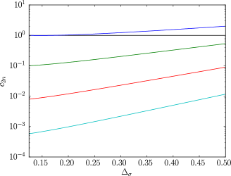
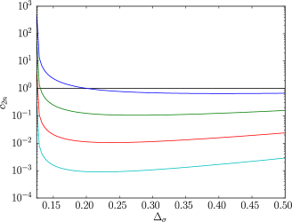
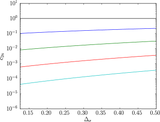
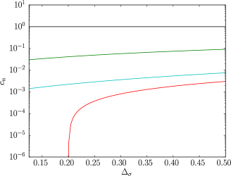
Figure 2: Log-scale plots of c2nϵϵ(1,s)ϵϵsubscriptsuperscript𝑐italic-ϵitalic-ϵ1𝑠italic-ϵitalic-ϵ2𝑛c^{\epsilon\epsilon(1,s)\epsilon\epsilon}_{2n} showing that the first five are all positive on the interval 18Δσ1218subscriptΔ𝜎12\frac{1}{8}\leq\Delta_{\sigma}\leq\frac{1}{2}.

The null state condition that follows from (3.30) and (3.31) is

4z2(z1)33Gz3+4z(z1)2[(4Δϵ)z+2Δϵ2]2Gz24superscript𝑧2superscript𝑧13superscript3𝐺superscript𝑧34𝑧superscript𝑧12delimited-[]4subscriptΔitalic-ϵ𝑧2subscriptΔitalic-ϵ2superscript2𝐺superscript𝑧2\displaystyle 4z^{2}(z-1)^{3}\frac{\partial^{3}G}{\partial z^{3}}+4z(z-1)^{2}[(4-\Delta_{\epsilon})z+2\Delta_{\epsilon}-2]\frac{\partial^{2}G}{\partial z^{2}}
(z1)[(Δϵ2+10Δϵ8)z2+(3Δϵ214Δϵ+8)z3Δϵ(Δϵ2)]Gz𝑧1delimited-[]superscriptsubscriptΔitalic-ϵ210subscriptΔitalic-ϵ8superscript𝑧23superscriptsubscriptΔitalic-ϵ214subscriptΔitalic-ϵ8𝑧3subscriptΔitalic-ϵsubscriptΔitalic-ϵ2𝐺𝑧\displaystyle-(z-1)[(\Delta_{\epsilon}^{2}+10\Delta_{\epsilon}-8)z^{2}+(3\Delta_{\epsilon}^{2}-14\Delta_{\epsilon}+8)z-3\Delta_{\epsilon}(\Delta_{\epsilon}-2)]\frac{\partial G}{\partial z}
+Δϵ2(Δϵ+2)z(z2)G=0.superscriptsubscriptΔitalic-ϵ2subscriptΔitalic-ϵ2𝑧𝑧2𝐺0\displaystyle+\Delta_{\epsilon}^{2}(\Delta_{\epsilon}+2)z(z-2)G=0\;. (3.32)

To approximate the Virasoro blocks that solve this, it will be helpful to use the Frobenius method.121212Even though they describe exchanged weights of h1,1subscript11h_{1,1} and h1,3subscript13h_{1,3}, we cannot reuse either of the expressions in (3.6). Unlike global blocks which only see dimension differences, Virasoro blocks depend on the external weights individually [42]. Inserting the ansatz G(z)=k=bkzr+k𝐺𝑧superscriptsubscript𝑘subscript𝑏𝑘superscript𝑧𝑟𝑘G(z)=\sum_{k=-\infty}^{\infty}b_{k}z^{r+k}, we may reindex the sum so that all terms carry the same power of z𝑧z. This gives a recurrence relation for the coefficients.

[4(k+r)(k+r1)+8(Δϵ1)(k+r)+3Δϵ(2Δϵ)](k+r+1)bk+1delimited-[]4𝑘𝑟𝑘𝑟18subscriptΔitalic-ϵ1𝑘𝑟3subscriptΔitalic-ϵ2subscriptΔitalic-ϵ𝑘𝑟1subscript𝑏𝑘1\displaystyle[-4(k+r)(k+r-1)+8(\Delta_{\epsilon}-1)(k+r)+3\Delta_{\epsilon}(2-\Delta_{\epsilon})](k+r+1)b_{k+1}
+2[6(k+r1)(k+r2)+2(85Δϵ)(k+r1)+3Δϵ210Δϵ+4](k+r)bk2delimited-[]6𝑘𝑟1𝑘𝑟2285subscriptΔitalic-ϵ𝑘𝑟13superscriptsubscriptΔitalic-ϵ210subscriptΔitalic-ϵ4𝑘𝑟subscript𝑏𝑘\displaystyle+2[6(k+r-1)(k+r-2)+2(8-5\Delta_{\epsilon})(k+r-1)+3\Delta_{\epsilon}^{2}-10\Delta_{\epsilon}+4](k+r)b_{k}
2[6(k+r1)(k+r2)(k+r3)4(2Δϵ5)(k+r1)(k+r2)\displaystyle-2\left[6(k+r-1)(k+r-2)(k+r-3)-4(2\Delta_{\epsilon}-5)(k+r-1)(k+r-2)\right.
+(Δϵ212Δϵ+8)(k+r1)+Δϵ2(Δϵ+2)]bk1\displaystyle\left.+(\Delta_{\epsilon}^{2}-12\Delta_{\epsilon}+8)(k+r-1)+\Delta_{\epsilon}^{2}(\Delta_{\epsilon}+2)\right]b_{k-1}
+[4(k+r2)(k+r3)(k+r4)+4(4Δϵ)(k+r2)(k+r3)\displaystyle+\left[4(k+r-2)(k+r-3)(k+r-4)+4(4-\Delta_{\epsilon})(k+r-2)(k+r-3)\right.
(Δϵ2+10Δϵ8)(k+r2)+Δϵ2(Δϵ+2)]bk2=0\displaystyle\left.-(\Delta_{\epsilon}^{2}+10\Delta_{\epsilon}-8)(k+r-2)+\Delta_{\epsilon}^{2}(\Delta_{\epsilon}+2)\right]b_{k-2}=0 (3.33)

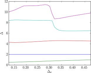
We will set b0=1subscript𝑏01b_{0}=1 and bk=0subscript𝑏𝑘0b_{k}=0 for all k<0𝑘0k<0. The values of r𝑟r that make this consistent (called roots of the indicial equation) are h1,1subscript11h_{1,1}, h1,3subscript13h_{1,3} and h1,5subscript15h_{1,5} as expected. We find them by demanding that b0subscript𝑏0b_{0} drop out of (3.33) when k=1𝑘1k=-1. For each value of r𝑟r, it is straightforward to iterate (3.33) and then feed the results into (2.5). Some of the OPE coefficients that follow from this are written in Table 3. Due to the appearance of the upper bound (1.4) in the three-correlator bootstrap, we expect the coefficients to be positive when 1Δϵ21subscriptΔitalic-ϵ21\leq\Delta_{\epsilon}\leq 2, at least up to some high order. Figure 2 shows that this is indeed the case.

n𝑛n c2nϵϵ(1,1)ϵϵsuperscriptsubscript𝑐2𝑛italic-ϵitalic-ϵ11italic-ϵitalic-ϵc_{2n}^{\epsilon\epsilon(1,1)\epsilon\epsilon}
00 111
111 Δϵ2(Δϵ+2)(Δϵ4)(3Δϵ2)superscriptsubscriptΔitalic-ϵ2subscriptΔitalic-ϵ2subscriptΔitalic-ϵ43subscriptΔitalic-ϵ2-\frac{\Delta_{\epsilon}^{2}(\Delta_{\epsilon}+2)}{(\Delta_{\epsilon}-4)(3\Delta_{\epsilon}-2)}
222 Δϵ2(Δϵ+2)2[5Δϵ+2]30(Δϵ8)(Δϵ4)(3Δϵ2)superscriptsubscriptΔitalic-ϵ2superscriptsubscriptΔitalic-ϵ22delimited-[]5subscriptΔitalic-ϵ230subscriptΔitalic-ϵ8subscriptΔitalic-ϵ43subscriptΔitalic-ϵ2\frac{\Delta_{\epsilon}^{2}(\Delta_{\epsilon}+2)^{2}[5\Delta_{\epsilon}+2]}{30(\Delta_{\epsilon}-8)(\Delta_{\epsilon}-4)(3\Delta_{\epsilon}-2)}
n𝑛n c2nϵϵ(3,1)ϵϵsuperscriptsubscript𝑐2𝑛italic-ϵitalic-ϵ31italic-ϵitalic-ϵc_{2n}^{\epsilon\epsilon(3,1)\epsilon\epsilon}
00 111
111 Δϵ2(Δϵ+2)[5Δϵ+2]16(Δϵ1)(Δϵ+1)(Δϵ+4)superscriptsubscriptΔitalic-ϵ2subscriptΔitalic-ϵ2delimited-[]5subscriptΔitalic-ϵ216subscriptΔitalic-ϵ1subscriptΔitalic-ϵ1subscriptΔitalic-ϵ4\frac{\Delta_{\epsilon}^{2}(\Delta_{\epsilon}+2)[5\Delta_{\epsilon}+2]}{16(\Delta_{\epsilon}-1)(\Delta_{\epsilon}+1)(\Delta_{\epsilon}+4)}
222 Δϵ2(Δϵ+2)[25Δϵ5+167Δϵ466Δϵ31904Δϵ22752Δϵ384]512(Δϵ3)(Δϵ1)(Δϵ+3)(Δϵ+4)(Δϵ+5)(Δϵ+8)superscriptsubscriptΔitalic-ϵ2subscriptΔitalic-ϵ2delimited-[]25superscriptsubscriptΔitalic-ϵ5167superscriptsubscriptΔitalic-ϵ466superscriptsubscriptΔitalic-ϵ31904superscriptsubscriptΔitalic-ϵ22752subscriptΔitalic-ϵ384512subscriptΔitalic-ϵ3subscriptΔitalic-ϵ1subscriptΔitalic-ϵ3subscriptΔitalic-ϵ4subscriptΔitalic-ϵ5subscriptΔitalic-ϵ8\frac{\Delta_{\epsilon}^{2}(\Delta_{\epsilon}+2)[25\Delta_{\epsilon}^{5}+167\Delta_{\epsilon}^{4}-66\Delta_{\epsilon}^{3}-1904\Delta_{\epsilon}^{2}-2752\Delta_{\epsilon}-384]}{512(\Delta_{\epsilon}-3)(\Delta_{\epsilon}-1)(\Delta_{\epsilon}+3)(\Delta_{\epsilon}+4)(\Delta_{\epsilon}+5)(\Delta_{\epsilon}+8)}
n𝑛n c2nϵϵ(5,1)ϵϵsuperscriptsubscript𝑐2𝑛italic-ϵitalic-ϵ51italic-ϵitalic-ϵc_{2n}^{\epsilon\epsilon(5,1)\epsilon\epsilon}
00 111
111 Δϵ(Δϵ+2)[7Δϵ+6]48(Δϵ+1)(Δϵ+3)subscriptΔitalic-ϵsubscriptΔitalic-ϵ2delimited-[]7subscriptΔitalic-ϵ648subscriptΔitalic-ϵ1subscriptΔitalic-ϵ3\frac{\Delta_{\epsilon}(\Delta_{\epsilon}+2)[7\Delta_{\epsilon}+6]}{48(\Delta_{\epsilon}+1)(\Delta_{\epsilon}+3)}
222 Δϵ(Δϵ+2)[441Δϵ5+5121Δϵ4+20732Δϵ3+37796Δϵ2+31056Δϵ+8640]1536(Δϵ+3)(Δϵ+5)(3Δϵ+5)(3Δϵ+7)(3Δϵ+10)subscriptΔitalic-ϵsubscriptΔitalic-ϵ2delimited-[]441superscriptsubscriptΔitalic-ϵ55121superscriptsubscriptΔitalic-ϵ420732superscriptsubscriptΔitalic-ϵ337796superscriptsubscriptΔitalic-ϵ231056subscriptΔitalic-ϵ86401536subscriptΔitalic-ϵ3subscriptΔitalic-ϵ53subscriptΔitalic-ϵ53subscriptΔitalic-ϵ73subscriptΔitalic-ϵ10\frac{\Delta_{\epsilon}(\Delta_{\epsilon}+2)[441\Delta_{\epsilon}^{5}+5121\Delta_{\epsilon}^{4}+20732\Delta_{\epsilon}^{3}+37796\Delta_{\epsilon}^{2}+31056\Delta_{\epsilon}+8640]}{1536(\Delta_{\epsilon}+3)(\Delta_{\epsilon}+5)(3\Delta_{\epsilon}+5)(3\Delta_{\epsilon}+7)(3\Delta_{\epsilon}+10)}
Table 3: The first three global block coefficients in the (1,1)11(1,1), (1,3)13(1,3) and (1,5)15(1,5) contributions found by taking the ϵ×ϵitalic-ϵitalic-ϵ\epsilon\times\epsilon OPE twice.

We should also be able to find positive squared OPE coefficients in the mixed correlator. The four-point function

σ(z1,z¯1)ϵ(z2,z¯2)σ(z3,z¯3)ϵ(z4,z¯4)=(|z24||z13|)ΔσϵG(z,z¯)|z12|Δσ+Δϵ|z34|Δσ+Δϵdelimited-⟨⟩𝜎subscript𝑧1subscript¯𝑧1italic-ϵsubscript𝑧2subscript¯𝑧2𝜎subscript𝑧3subscript¯𝑧3italic-ϵsubscript𝑧4subscript¯𝑧4superscriptsubscript𝑧24subscript𝑧13subscriptΔ𝜎italic-ϵ𝐺𝑧¯𝑧superscriptsubscript𝑧12subscriptΔ𝜎subscriptΔitalic-ϵsuperscriptsubscript𝑧34subscriptΔ𝜎subscriptΔitalic-ϵ\displaystyle\left<\sigma(z_{1},\bar{z}_{1})\epsilon(z_{2},\bar{z}_{2})\sigma(z_{3},\bar{z}_{3})\epsilon(z_{4},\bar{z}_{4})\right>=\left(\frac{|z_{24}|}{|z_{13}|}\right)^{\Delta_{\sigma\epsilon}}\frac{G(z,\bar{z})}{|z_{12}|^{\Delta_{\sigma}+\Delta_{\epsilon}}|z_{34}|^{\Delta_{\sigma}+\Delta_{\epsilon}}}
G(z,z¯)=C(1,2)(1,3)(1,2)G(1,2)σϵσϵ(z)G(1,2)σϵσϵ(z¯)+C(1,2)(1,3)(1,4)G(1,4)σϵσϵ(z)G(1,4)σϵσϵ(z¯)𝐺𝑧¯𝑧subscriptsuperscript𝐶121213subscriptsuperscript𝐺𝜎italic-ϵ𝜎italic-ϵ12𝑧subscriptsuperscript𝐺𝜎italic-ϵ𝜎italic-ϵ12¯𝑧subscriptsuperscript𝐶141213subscriptsuperscript𝐺𝜎italic-ϵ𝜎italic-ϵ14𝑧subscriptsuperscript𝐺𝜎italic-ϵ𝜎italic-ϵ14¯𝑧\displaystyle G(z,\bar{z})=C^{(1,2)}_{(1,2)(1,3)}G^{\sigma\epsilon\sigma\epsilon}_{(1,2)}(z)G^{\sigma\epsilon\sigma\epsilon}_{(1,2)}(\bar{z})+C^{(1,4)}_{(1,2)(1,3)}G^{\sigma\epsilon\sigma\epsilon}_{(1,4)}(z)G^{\sigma\epsilon\sigma\epsilon}_{(1,4)}(\bar{z}) (3.34)

satisfies second-order and third-order BPZ equations.
Refer to caption
(a)
Refer to caption
(b)
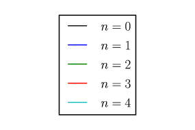
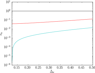
Figure 3: Log-scale plots of the cnσϵ(1,s)σϵsubscriptsuperscript𝑐𝜎italic-ϵ1𝑠𝜎italic-ϵ𝑛c^{\sigma\epsilon(1,s)\sigma\epsilon}_{n} that are non-zero. The legend is the same as that of Figure 2.

For simplicity, we will consider the second-order equation

32z2(z1)22Gz2+12z(z1)[(27Δσ)z+9Δσ]Gz32superscript𝑧2superscript𝑧12superscript2𝐺superscript𝑧212𝑧𝑧1delimited-[]27subscriptΔ𝜎𝑧9subscriptΔ𝜎𝐺𝑧\displaystyle\frac{3}{2}z^{2}(z-1)^{2}\frac{\partial^{2}G}{\partial z^{2}}+\frac{1}{2}z(z-1)[(2-7\Delta_{\sigma})z+9\Delta_{\sigma}]\frac{\partial G}{\partial z}
+124[3Δσ(11Δσ+2)z22(5Δσ+2)(11Δσ+2)z+9Δσ(5Δσ+2)]G=0124delimited-[]3subscriptΔ𝜎11subscriptΔ𝜎2superscript𝑧225subscriptΔ𝜎211subscriptΔ𝜎2𝑧9subscriptΔ𝜎5subscriptΔ𝜎2𝐺0\displaystyle+\frac{1}{24}[3\Delta_{\sigma}(11\Delta_{\sigma}+2)z^{2}-2(5\Delta_{\sigma}+2)(11\Delta_{\sigma}+2)z+9\Delta_{\sigma}(5\Delta_{\sigma}+2)]G=0 (3.35)

which has the recurrence relation

9[4(k+r+1)(k+r)12Δσ(k+r+1)+Δσ(5Δσ+2)]bk+19delimited-[]4𝑘𝑟1𝑘𝑟12subscriptΔ𝜎𝑘𝑟1subscriptΔ𝜎5subscriptΔ𝜎2subscript𝑏𝑘1\displaystyle 9[4(k+r+1)(k+r)-12\Delta_{\sigma}(k+r+1)+\Delta_{\sigma}(5\Delta_{\sigma}+2)]b_{k+1} (3.36)
2[36(k+r)(k+r1)12(8Δσ1)(k+r)+(5Δσ+2)(11Δσ+2)]bk2delimited-[]36𝑘𝑟𝑘𝑟1128subscriptΔ𝜎1𝑘𝑟5subscriptΔ𝜎211subscriptΔ𝜎2subscript𝑏𝑘\displaystyle-2[36(k+r)(k+r-1)-12(8\Delta_{\sigma}-1)(k+r)+(5\Delta_{\sigma}+2)(11\Delta_{\sigma}+2)]b_{k}
+3[12(k+r1)(k+r2)+4(27Δσ)(k+r1)+Δσ(11Δσ+2)]bk1=0.3delimited-[]12𝑘𝑟1𝑘𝑟2427subscriptΔ𝜎𝑘𝑟1subscriptΔ𝜎11subscriptΔ𝜎2subscript𝑏𝑘10\displaystyle+3[12(k+r-1)(k+r-2)+4(2-7\Delta_{\sigma})(k+r-1)+\Delta_{\sigma}(11\Delta_{\sigma}+2)]b_{k-1}=0\;.

It is easily seen that r{h1,2,h1,4}𝑟subscript12subscript14r\in\{h_{1,2},h_{1,4}\} is the solution of the indicial equation for (3.36). Because the product σ×ϵ𝜎italic-ϵ\sigma\times\epsilon no longer has Bose symmetry, the procedure by which we extract the conformal block expansion this time is somewhat different. We must include dimension differences in the hypergeometric function and sum over all integers whether even or odd.

G(z)𝐺𝑧\displaystyle G(z) =\displaystyle= n=0(1)ncnzr+nF12(r+n12Δσϵ,r+n+12Δσϵ;2(r+n);z)superscriptsubscript𝑛0superscript1𝑛subscript𝑐𝑛superscript𝑧𝑟𝑛subscriptsubscript𝐹12𝑟𝑛12subscriptΔ𝜎italic-ϵ𝑟𝑛12subscriptΔ𝜎italic-ϵ2𝑟𝑛𝑧\displaystyle\sum_{n=0}^{\infty}(-1)^{n}c_{n}z^{r+n}{}_{2}F_{1}\left(r+n-\frac{1}{2}\Delta_{\sigma\epsilon},r+n+\frac{1}{2}\Delta_{\sigma\epsilon};2(r+n);z\right) (3.37)
=\displaystyle= n=0m=0(1)ncn(r+n12Δσϵ)m(r+n+12Δσϵ)m(2r+2n)mzr+n+mm!superscriptsubscript𝑛0superscriptsubscript𝑚0superscript1𝑛subscript𝑐𝑛subscript𝑟𝑛12subscriptΔ𝜎italic-ϵ𝑚subscript𝑟𝑛12subscriptΔ𝜎italic-ϵ𝑚subscript2𝑟2𝑛𝑚superscript𝑧𝑟𝑛𝑚𝑚\displaystyle\sum_{n=0}^{\infty}\sum_{m=0}^{\infty}(-1)^{n}c_{n}\frac{\left(r+n-\frac{1}{2}\Delta_{\sigma\epsilon}\right)_{m}\left(r+n+\frac{1}{2}\Delta_{\sigma\epsilon}\right)_{m}}{(2r+2n)_{m}}\frac{z^{r+n+m}}{m!}
=\displaystyle= k=0n=0k(1)ncn(r+n12Δσϵ)kn(r+n+12Δσϵ)kn(2r+2n)knzr+k(kn)!superscriptsubscript𝑘0superscriptsubscript𝑛0𝑘superscript1𝑛subscript𝑐𝑛subscript𝑟𝑛12subscriptΔ𝜎italic-ϵ𝑘𝑛subscript𝑟𝑛12subscriptΔ𝜎italic-ϵ𝑘𝑛subscript2𝑟2𝑛𝑘𝑛superscript𝑧𝑟𝑘𝑘𝑛\displaystyle\sum_{k=0}^{\infty}\sum_{n=0}^{k}(-1)^{n}c_{n}\frac{\left(r+n-\frac{1}{2}\Delta_{\sigma\epsilon}\right)_{k-n}\left(r+n+\frac{1}{2}\Delta_{\sigma\epsilon}\right)_{k-n}}{(2r+2n)_{k-n}}\frac{z^{r+k}}{(k-n)!}

The lower triangular system from this leads to the recursion

(1)kck=bkn=0k1(1)ncn(r+n12Δσϵ)kn(r+n+12Δσϵ)kn(2r+2n)kn(kn)!.superscript1𝑘subscript𝑐𝑘subscript𝑏𝑘superscriptsubscript𝑛0𝑘1superscript1𝑛subscript𝑐𝑛subscript𝑟𝑛12subscriptΔ𝜎italic-ϵ𝑘𝑛subscript𝑟𝑛12subscriptΔ𝜎italic-ϵ𝑘𝑛subscript2𝑟2𝑛𝑘𝑛𝑘𝑛(-1)^{k}c_{k}=b_{k}-\sum_{n=0}^{k-1}(-1)^{n}c_{n}\frac{\left(r+n-\frac{1}{2}\Delta_{\sigma\epsilon}\right)_{k-n}\left(r+n+\frac{1}{2}\Delta_{\sigma\epsilon}\right)_{k-n}}{(2r+2n)_{k-n}(k-n)!}\;. (3.38)
n𝑛n cnσϵ(1,2)σϵsuperscriptsubscript𝑐𝑛𝜎italic-ϵ12𝜎italic-ϵc_{n}^{\sigma\epsilon(1,2)\sigma\epsilon}
00 111
111 00
222 00
333 (Δσ+1)(4Δσ+1)2729Δσ(Δσ1)(Δσ+2)(5Δσ+2)subscriptΔ𝜎1superscript4subscriptΔ𝜎12729subscriptΔ𝜎subscriptΔ𝜎1subscriptΔ𝜎25subscriptΔ𝜎2-\frac{(\Delta_{\sigma}+1)(4\Delta_{\sigma}+1)^{2}}{729\Delta_{\sigma}(\Delta_{\sigma}-1)(\Delta_{\sigma}+2)}(5\Delta_{\sigma}+2)
444 4(Δσ+1)2(4Δσ+1)2729Δσ(Δσ+3)(Δσ+6)(2Δσ3)(8Δσ1)4superscriptsubscriptΔ𝜎12superscript4subscriptΔ𝜎12729subscriptΔ𝜎subscriptΔ𝜎3subscriptΔ𝜎62subscriptΔ𝜎38subscriptΔ𝜎1-\frac{4(\Delta_{\sigma}+1)^{2}(4\Delta_{\sigma}+1)^{2}}{729\Delta_{\sigma}(\Delta_{\sigma}+3)(\Delta_{\sigma}+6)(2\Delta_{\sigma}-3)}(8\Delta_{\sigma}-1)
n𝑛n cnσϵ(1,4)σϵsuperscriptsubscript𝑐𝑛𝜎italic-ϵ14𝜎italic-ϵc_{n}^{\sigma\epsilon(1,4)\sigma\epsilon}
00 111
111 00
222 Δσ+19(2Δσ+3)(5Δσ+3)(2Δσ+1)(10Δσ+1)subscriptΔ𝜎192subscriptΔ𝜎35subscriptΔ𝜎32subscriptΔ𝜎110subscriptΔ𝜎1\frac{\Delta_{\sigma}+1}{9(2\Delta_{\sigma}+3)(5\Delta_{\sigma}+3)}(2\Delta_{\sigma}+1)(10\Delta_{\sigma}+1)
333 4(Δσ+1)(5Δσ+2)729(Δσ+2)(5Δσ+4)(5Δσ+6)(5Δσ1)(7Δσ+4)4subscriptΔ𝜎15subscriptΔ𝜎2729subscriptΔ𝜎25subscriptΔ𝜎45subscriptΔ𝜎65subscriptΔ𝜎17subscriptΔ𝜎4\frac{4(\Delta_{\sigma}+1)(5\Delta_{\sigma}+2)}{729(\Delta_{\sigma}+2)(5\Delta_{\sigma}+4)(5\Delta_{\sigma}+6)}(5\Delta_{\sigma}-1)(7\Delta_{\sigma}+4)
444 (Δσ+1)2(5Δσ+2)81(5Δσ+7)(5Δσ+8)(10Δσ+1)superscriptsubscriptΔ𝜎125subscriptΔ𝜎2815subscriptΔ𝜎75subscriptΔ𝜎810subscriptΔ𝜎1\frac{(\Delta_{\sigma}+1)^{2}(5\Delta_{\sigma}+2)}{81(5\Delta_{\sigma}+7)(5\Delta_{\sigma}+8)}(10\Delta_{\sigma}+1)
Table 4: The first five global block coefficients in the (1,2)12(1,2) and (1,4)14(1,4) contributions found by taking the σ×ϵ𝜎italic-ϵ\sigma\times\epsilon OPE twice.

Some low-lying global block coefficients found with (3.38) are listed in Table 4. While all of them are non-negative above the tricritical Ising value Δσ=15subscriptΔ𝜎15\Delta_{\sigma}=\frac{1}{5}, there is actually one that takes on negative values for 18<Δσ<1518subscriptΔ𝜎15\frac{1}{8}<\Delta_{\sigma}<\frac{1}{5} as shown in Figure 3. We may explain this by noticing that ϕ1,4subscriptitalic-ϕ14\phi_{1,4} is also ϕ3,1subscriptitalic-ϕ31\phi_{3,1} in the minimal model (5,4)54\mathcal{M}(5,4). This field has exactly one quasiprimary descendant at level 3. The presence of a null state is therefore enough to conclude that c3σϵ(1,4)σϵ=0subscriptsuperscript𝑐𝜎italic-ϵ14𝜎italic-ϵ30c^{\sigma\epsilon(1,4)\sigma\epsilon}_{3}=0.

n𝑛n c2nσσ(1,1)ϵϵsuperscriptsubscript𝑐2𝑛𝜎𝜎11italic-ϵitalic-ϵc_{2n}^{\sigma\sigma(1,1)\epsilon\epsilon}
00 111
111 (Δσ+1)(4Δσ+1)3(54Δσ)subscriptΔ𝜎14subscriptΔ𝜎1354subscriptΔ𝜎\frac{(\Delta_{\sigma}+1)(4\Delta_{\sigma}+1)}{3(5-4\Delta_{\sigma})}
222 2(Δσ+1)2(4Δσ+1)[5Δσ+2]45(54Δσ)(114Δσ)2superscriptsubscriptΔ𝜎124subscriptΔ𝜎1delimited-[]5subscriptΔ𝜎24554subscriptΔ𝜎114subscriptΔ𝜎\frac{2(\Delta_{\sigma}+1)^{2}(4\Delta_{\sigma}+1)[5\Delta_{\sigma}+2]}{45(5-4\Delta_{\sigma})(11-4\Delta_{\sigma})}
n𝑛n c2nσσ(1,3)ϵϵsuperscriptsubscript𝑐2𝑛𝜎𝜎13italic-ϵitalic-ϵc_{2n}^{\sigma\sigma(1,3)\epsilon\epsilon}
00 111
111 2(Δσ+1)(4Δσ+1)[5Δσ+2]3(7+4Δσ)(5+8Δσ)2subscriptΔ𝜎14subscriptΔ𝜎1delimited-[]5subscriptΔ𝜎2374subscriptΔ𝜎58subscriptΔ𝜎\frac{2(\Delta_{\sigma}+1)(4\Delta_{\sigma}+1)[5\Delta_{\sigma}+2]}{3(7+4\Delta_{\sigma})(5+8\Delta_{\sigma})}
222 (Δσ+1)2(4Δσ+1)[400Δσ3+1548Δσ2+1644Δσ+361]18(7+4Δσ)(13+4Δσ)(11+8Δσ)(17+8Δσ)superscriptsubscriptΔ𝜎124subscriptΔ𝜎1delimited-[]400superscriptsubscriptΔ𝜎31548superscriptsubscriptΔ𝜎21644subscriptΔ𝜎3611874subscriptΔ𝜎134subscriptΔ𝜎118subscriptΔ𝜎178subscriptΔ𝜎\frac{(\Delta_{\sigma}+1)^{2}(4\Delta_{\sigma}+1)[400\Delta_{\sigma}^{3}+1548\Delta_{\sigma}^{2}+1644\Delta_{\sigma}+361]}{18(7+4\Delta_{\sigma})(13+4\Delta_{\sigma})(11+8\Delta_{\sigma})(17+8\Delta_{\sigma})}
Table 5: The first three global block coefficients in the (1,1)11(1,1) and (1,3)13(1,3) contributions found by taking the σ×σ𝜎𝜎\sigma\times\sigma and ϵ×ϵitalic-ϵitalic-ϵ\epsilon\times\epsilon OPEs.

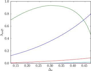
Alternatively, we can take the OPE in the other channel by permuting operator positions in (3.34). This yields the global block coefficients in Table 5 which are related to the λσσ𝒪λϵϵ𝒪subscript𝜆𝜎𝜎𝒪subscript𝜆italic-ϵitalic-ϵ𝒪\lambda_{\sigma\sigma\mathcal{O}}\lambda_{\epsilon\epsilon\mathcal{O}} CFT data. There is no reason for these numbers to be positive, but we expect

c2nσσ(1,s)σσc2nϵϵ(1,s)ϵϵ(c2nσσ(1,s)ϵϵ)2subscriptsuperscript𝑐𝜎𝜎1𝑠𝜎𝜎2𝑛subscriptsuperscript𝑐italic-ϵitalic-ϵ1𝑠italic-ϵitalic-ϵ2𝑛superscriptsubscriptsuperscript𝑐𝜎𝜎1𝑠italic-ϵitalic-ϵ2𝑛2c^{\sigma\sigma(1,s)\sigma\sigma}_{2n}c^{\epsilon\epsilon(1,s)\epsilon\epsilon}_{2n}\geq\left(c^{\sigma\sigma(1,s)\epsilon\epsilon}_{2n}\right)^{2} (3.39)

to be obeyed.131313For another quick check of our results, Δϵ2c0σσ(1,1)σσc2σσ(1,1)σσ=Δσ2c0ϵϵ(1,1)ϵϵc2ϵϵ(1,1)ϵϵsuperscriptsubscriptΔitalic-ϵ2subscriptsuperscript𝑐𝜎𝜎11𝜎𝜎0subscriptsuperscript𝑐𝜎𝜎11𝜎𝜎2superscriptsubscriptΔ𝜎2subscriptsuperscript𝑐italic-ϵitalic-ϵ11italic-ϵitalic-ϵ0subscriptsuperscript𝑐italic-ϵitalic-ϵ11italic-ϵitalic-ϵ2\Delta_{\epsilon}^{2}c^{\sigma\sigma(1,1)\sigma\sigma}_{0}c^{\sigma\sigma(1,1)\sigma\sigma}_{2}=\Delta_{\sigma}^{2}c^{\epsilon\epsilon(1,1)\epsilon\epsilon}_{0}c^{\epsilon\epsilon(1,1)\epsilon\epsilon}_{2} holds as it must by the Ward identity. When σ×σ𝜎𝜎\sigma\times\sigma and ϵ×ϵitalic-ϵitalic-ϵ\epsilon\times\epsilon share a set of operators 𝒮𝒮\mathcal{S} with the same quantum numbers, the left-hand side is a product of sums. The right-hand side is a sum of products and therefore smaller by the arithmetic-geometric mean inequality. A departure from (3.39) would be a violation of unitarity since the matrix

𝒪𝒮[λσσ𝒪λϵϵ𝒪][λσσ𝒪λϵϵ𝒪]=[cσσ(1,s)σσ2ncσσ(1,s)ϵϵ2ncσσ(1,s)ϵϵ2ncϵϵ(1,s)ϵϵ2n]subscript𝒪𝒮delimited-[]subscript𝜆𝜎𝜎𝒪subscript𝜆italic-ϵitalic-ϵ𝒪delimited-[]fragmentsλ𝜎𝜎𝒪fragmentsλitalic-ϵitalic-ϵ𝒪delimited-[]fragmentsc𝜎𝜎1𝑠𝜎𝜎2𝑛fragmentsc𝜎𝜎1𝑠italic-ϵitalic-ϵ2𝑛fragmentsc𝜎𝜎1𝑠italic-ϵitalic-ϵ2𝑛fragmentscitalic-ϵitalic-ϵ1𝑠italic-ϵitalic-ϵ2𝑛\sum_{\mathcal{O}\in\mathcal{S}}\left[\lambda_{\sigma\sigma\mathcal{O}}\;\lambda_{\epsilon\epsilon\mathcal{O}}\right]\left[\begin{tabular}[]{c}$\lambda_{\sigma\sigma\mathcal{O}}$\\ $\lambda_{\epsilon\epsilon\mathcal{O}}$\end{tabular}\right]=\left[\begin{tabular}[]{cc}$c^{\sigma\sigma(1,s)\sigma\sigma}_{2n}$&$c^{\sigma\sigma(1,s)\epsilon\epsilon}_{2n}$\\ $c^{\sigma\sigma(1,s)\epsilon\epsilon}_{2n}$&$c^{\epsilon\epsilon(1,s)\epsilon\epsilon}_{2n}$\end{tabular}\right] (3.40)

would not be positive-definite.

3.3 Virasoro block coefficients

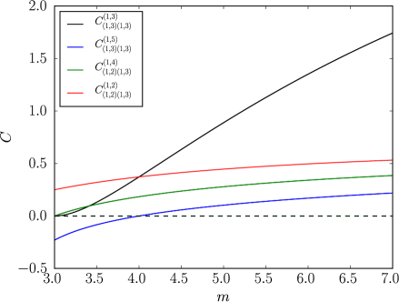
Our analysis so far has been focused on c2nσσ(1,s)σσsubscriptsuperscript𝑐𝜎𝜎1𝑠𝜎𝜎2𝑛c^{\sigma\sigma(1,s)\sigma\sigma}_{2n}, c2nϵϵ(1,s)ϵϵsubscriptsuperscript𝑐italic-ϵitalic-ϵ1𝑠italic-ϵitalic-ϵ2𝑛c^{\epsilon\epsilon(1,s)\epsilon\epsilon}_{2n} and cnσϵ(1,s)σϵsubscriptsuperscript𝑐𝜎italic-ϵ1𝑠𝜎italic-ϵ𝑛c^{\sigma\epsilon(1,s)\sigma\epsilon}_{n}, which encode the decomposition of a Virasoro block into 𝔰𝔩(2)𝔰𝔩2\mathfrak{sl}(2) blocks. With the sole exception of c3σϵ(1,4)σϵsubscriptsuperscript𝑐𝜎italic-ϵ14𝜎italic-ϵ3c^{\sigma\epsilon(1,4)\sigma\epsilon}_{3}, which we could imagine to have a small effect, we have found that these coefficients are non-negative when 18Δσ1218subscriptΔ𝜎12\frac{1}{8}\leq\Delta_{\sigma}\leq\frac{1}{2}. However, this is only meaningful if the same property holds for the structure constants that unite holomorphic and anti-holomorphic halves of a four-point function. A single C(r1,s1)(r2,s2)(r3,s3)<0superscriptsubscript𝐶subscript𝑟1subscript𝑠1subscript𝑟2subscript𝑠2subscript𝑟3subscript𝑠30C_{(r_{1},s_{1})(r_{2},s_{2})}^{(r_{3},s_{3})}<0 for instance would give rise to an infintie number of negative contributions in ϕr1,s1ϕr2,s2ϕr1,s1ϕr2,s2delimited-⟨⟩subscriptitalic-ϕsubscript𝑟1subscript𝑠1subscriptitalic-ϕsubscript𝑟2subscript𝑠2subscriptitalic-ϕsubscript𝑟1subscript𝑠1subscriptitalic-ϕsubscript𝑟2subscript𝑠2\left<\phi_{r_{1},s_{1}}\phi_{r_{2},s_{2}}\phi_{r_{1},s_{1}}\phi_{r_{2},s_{2}}\right>, severely complicating the interpretation of Figure 1.

In a given correlation function, the Virasoro block coefficients that appear must be compatible with crossing symmetry and single-valuedness. By briefly reviewing the method of [38, 39, 40], we will show that this condition is enough to fix them uniquely. For definiteness, consider the ϵϵϵϵdelimited-⟨⟩italic-ϵitalic-ϵitalic-ϵitalic-ϵ\left<\epsilon\epsilon\epsilon\epsilon\right> correlator in the generalized minimal model with central charge 13211321\frac{13}{21}. The holomorphic part of this function comes from the kernel of the operator (3.31), which is three-dimensional. Solving (3.33) has given us a basis for this kernel in which each function vanishes at z=0𝑧0z=0. We could equally well have chosen any of the regular singular points 00, 111 and \infty, corresponding to the s𝑠s, t𝑡t and u𝑢u channels for Virasoro blocks. When going from z=0𝑧0z=0 to z=1𝑧1z=1, there is a special matrix F𝐹F called the crossing matrix (or fusion matrix) that accomplishes Ga(z)=FbaGb(1z)superscript𝐺𝑎𝑧subscriptsuperscript𝐹𝑎𝑏superscript𝐺𝑏1𝑧G^{a}(z)=F^{a}_{\;\;\;b}G^{b}(1-z). It is a special case of the crossing kernel which applies to theories with a continuous spectrum.141414Several interchangeable terms have proliferated over the years. When replacing the z1zmaps-to𝑧1𝑧z\mapsto 1-z map with z1zmaps-to𝑧1𝑧z\mapsto\frac{1}{z}, the words crossing and fusion become exchange and braiding. Outside the CFT context, one says that a linear ODE has a monodromy matrix or connection matrix. For ODEs that have less structure than a BPZ equation, finding this matrix is often a difficult problem. Since it represents a change of basis, the expression for F𝐹F is unique. In this case, it is given by

F=[0.74220.31240.15632.37621.87951.44051.87602.27332.1372],𝐹delimited-[]0.74220.3124fragments0.15632.3762fragments1.87951.44051.8760fragments2.27332.1372F=\left[\begin{tabular}[]{ccc}$0.7422$&$0.3124$&$-0.1563$\\ $2.3762$&$-1.8795$&$1.4405$\\ $1.8760$&$-2.2733$&$2.1372$\end{tabular}\right]\;, (3.41)

which was obtained in [43] via the Coulomb gas formalism. Later reviews are [44, 23]. In the following, we will use G1superscript𝐺1G^{1}, G2superscript𝐺2G^{2} and G3superscript𝐺3G^{3} to denote G(1,1)ϵϵϵϵsubscriptsuperscript𝐺italic-ϵitalic-ϵitalic-ϵitalic-ϵ11G^{\epsilon\epsilon\epsilon\epsilon}_{(1,1)}, G(1,3)ϵϵϵϵsubscriptsuperscript𝐺italic-ϵitalic-ϵitalic-ϵitalic-ϵ13G^{\epsilon\epsilon\epsilon\epsilon}_{(1,3)} and G(1,5)ϵϵϵϵsubscriptsuperscript𝐺italic-ϵitalic-ϵitalic-ϵitalic-ϵ15G^{\epsilon\epsilon\epsilon\epsilon}_{(1,5)} respectively.

The constraints from (3.41) are best phrased in terms of a metric on the space of conformal blocks; G(z,z¯)=WabGa(z)Gb(z¯)𝐺𝑧¯𝑧subscript𝑊𝑎𝑏superscript𝐺𝑎𝑧superscript𝐺𝑏¯𝑧G(z,\bar{z})=W_{ab}G^{a}(z)G^{b}(\bar{z}). We have three conditions that Wabsubscript𝑊𝑎𝑏W_{ab} must satisfy:

  1. 1.

    W11=1subscript𝑊111W_{11}=1

  2. 2.

    Wcd=WabFcaFdbsubscript𝑊𝑐𝑑subscript𝑊𝑎𝑏subscriptsuperscript𝐹𝑎𝑐subscriptsuperscript𝐹𝑏𝑑W_{cd}=W_{ab}F^{a}_{\;\;\;c}F^{b}_{\;\;\;d}

  3. 3.

    Wab=0subscript𝑊𝑎𝑏0W_{ab}=0 for ab𝑎𝑏a\neq b

The first of these is an obvious consequence of having unit-normalized operators. The second comes from writing G(1z,1z¯)=WabGa(1z)Gb(1z¯)𝐺1𝑧1¯𝑧subscript𝑊𝑎𝑏superscript𝐺𝑎1𝑧superscript𝐺𝑏1¯𝑧G(1-z,1-\bar{z})=W_{ab}G^{a}(1-z)G^{b}(1-\bar{z}) in terms of s𝑠s-channel blocks and setting it equal to G(z,z¯)𝐺𝑧¯𝑧G(z,\bar{z}). The third ensures that the four-point function has trivial monodromy under ze2πizmaps-to𝑧superscript𝑒2𝜋𝑖𝑧z\mapsto e^{2\pi i}z, z¯e2πiz¯maps-to¯𝑧superscript𝑒2𝜋𝑖¯𝑧\bar{z}\mapsto e^{-2\pi i}\bar{z}. This rules out a non-diagonal metric since we only find hr,ssubscript𝑟𝑠h_{r,s} weights that differ by integers at special values of m𝑚m.151515It is well known that this happens in discrete minimal models. Some of the non-diagonal theories so constructed also satisfy the stronger requirement of modular invariance. We build solutions out of the left eigenvectors of F𝐹F,

v1=[0.95370.11570.2776],v2=[0.98050.17580.0879],v3=[0.59380.71960.3600],formulae-sequencesuperscript𝑣1delimited-[]0.9537fragments0.11570.2776formulae-sequencesuperscript𝑣2delimited-[]0.98050.1758fragments0.0879superscript𝑣3delimited-[]0.5938fragments0.71960.3600v^{1}=\left[\begin{tabular}[]{c}$0.9537$\\ $-0.1157$\\ $0.2776$\end{tabular}\right]\;,\;v^{2}=\left[\begin{tabular}[]{c}$0.9805$\\ $0.1758$\\ $-0.0879$\end{tabular}\right]\;,\;v^{3}=\left[\begin{tabular}[]{c}$0.5938$\\ $-0.7196$\\ $0.3600$\end{tabular}\right]\;, (3.42)

which have eigenvalues of 111, 111 and 11-1 respectively. Clearly F2=1superscript𝐹21F^{2}=1, which follows from z1z𝑧1𝑧z\leftrightarrow 1-z being an involution, requires all eigenvalues to be ±1plus-or-minus1\pm 1. The following form is invariant under two multiplications by F𝐹F:

Wab=c11va1vb1+c12va1vb2+c21va2vb1+c22va2vb2+c33va3vb3.subscript𝑊𝑎𝑏subscript𝑐11subscriptsuperscript𝑣1𝑎subscriptsuperscript𝑣1𝑏subscript𝑐12subscriptsuperscript𝑣1𝑎subscriptsuperscript𝑣2𝑏subscript𝑐21subscriptsuperscript𝑣2𝑎subscriptsuperscript𝑣1𝑏subscript𝑐22subscriptsuperscript𝑣2𝑎subscriptsuperscript𝑣2𝑏subscript𝑐33subscriptsuperscript𝑣3𝑎subscriptsuperscript𝑣3𝑏W_{ab}=c_{11}v^{1}_{a}v^{1}_{b}+c_{12}v^{1}_{a}v^{2}_{b}+c_{21}v^{2}_{a}v^{1}_{b}+c_{22}v^{2}_{a}v^{2}_{b}+c_{33}v^{3}_{a}v^{3}_{b}\;. (3.43)

There are six off-diagonal components of W𝑊W that need to vanish. If we set c21=c12subscript𝑐21subscript𝑐12c_{21}=c_{12}, (3.43) becomes manifestly symmetric and we can use three more parameters, c11subscript𝑐11c_{11}, c12subscript𝑐12c_{12} and c22subscript𝑐22c_{22}, to make W𝑊W diagonal. As the single remaining parameter, c33subscript𝑐33c_{33} is used to rescale W𝑊W so that its leading component is 111.

Refer to caption
Figure 4: Low-lying squared OPE coefficients for Virasoro primaries in the generalized minimal models. Between the Ising model at m=3𝑚3m=3 (Δσ=18subscriptΔ𝜎18\Delta_{\sigma}=\frac{1}{8}) and the tricritical Ising model at m=4𝑚4m=4 (Δσ=15subscriptΔ𝜎15\Delta_{\sigma}=\frac{1}{5}), there is one that becomes negative.

We may summarize this discussion by stating that there is no freedom in the three-correlator bootstrap equations once the Virasoro blocks involving σ𝜎\sigma and ϵitalic-ϵ\epsilon are specified. Knowledge of these blocks fully determines σσσσdelimited-⟨⟩𝜎𝜎𝜎𝜎\left<\sigma\sigma\sigma\sigma\right>, σσϵϵdelimited-⟨⟩𝜎𝜎italic-ϵitalic-ϵ\left<\sigma\sigma\epsilon\epsilon\right> and ϵϵϵϵdelimited-⟨⟩italic-ϵitalic-ϵitalic-ϵitalic-ϵ\left<\epsilon\epsilon\epsilon\epsilon\right>, whether or not we demand consistency conditions for other correlators. This means that the generalized minimal model structure constants are the only valid choices for the coefficients in (3.3), (3.30) and (3.34). Defining γ(x)=Γ(x)/Γ(1x)𝛾𝑥Γ𝑥Γ1𝑥\gamma(x)=\Gamma(x)/\Gamma(1-x) and t=mm+1𝑡𝑚𝑚1t=\frac{m}{m+1}, the expressions we need are

C(1,3)(1,3)(1,3)subscriptsuperscript𝐶131313\displaystyle C^{(1,3)}_{(1,3)(1,3)} =\displaystyle= γ(t)3γ(4t1)2γ(12t)3γ(22t)γ(23t)𝛾superscript𝑡3𝛾superscript4𝑡12𝛾superscript12𝑡3𝛾22𝑡𝛾23𝑡\displaystyle\gamma(t)^{3}\gamma(4t-1)^{2}\gamma(1-2t)^{3}\gamma(2-2t)\gamma(2-3t)
C(1,3)(1,3)(1,5)subscriptsuperscript𝐶151313\displaystyle C^{(1,5)}_{(1,3)(1,3)} =\displaystyle= γ(t)γ(2t)γ(4t1)γ(5t1)γ(13t)γ(14t)γ(22t)γ(23t)𝛾𝑡𝛾2𝑡𝛾4𝑡1𝛾5𝑡1𝛾13𝑡𝛾14𝑡𝛾22𝑡𝛾23𝑡\displaystyle\gamma(t)\gamma(2t)\gamma(4t-1)\gamma(5t-1)\gamma(1-3t)\gamma(1-4t)\gamma(2-2t)\gamma(2-3t)
C(1,2)(1,3)(1,4)subscriptsuperscript𝐶141213\displaystyle C^{(1,4)}_{(1,2)(1,3)} =\displaystyle= γ(t)γ(4t1)γ(13t)γ(22t)𝛾𝑡𝛾4𝑡1𝛾13𝑡𝛾22𝑡\displaystyle\gamma(t)\gamma(4t-1)\gamma(1-3t)\gamma(2-2t)
C(1,2)(1,3)(1,2)subscriptsuperscript𝐶121213\displaystyle C^{(1,2)}_{(1,2)(1,3)} =\displaystyle= C(1,2)(1,2)(1,3)=γ(t)γ(3t1)γ(12t)γ(22t).subscriptsuperscript𝐶131212𝛾𝑡𝛾3𝑡1𝛾12𝑡𝛾22𝑡\displaystyle C^{(1,3)}_{(1,2)(1,2)}=\gamma(t)\gamma(3t-1)\gamma(1-2t)\gamma(2-2t)\;. (3.44)

The last coefficient in (3.44) is clearly the one that was rederived in [17]. Plotting these in Figure 4, we see that C(1,3)(1,3)(1,5)<0subscriptsuperscript𝐶1513130C^{(1,5)}_{(1,3)(1,3)}<0 for the generalized minimal models between (4,3)43\mathcal{M}(4,3) and (5,4)54\mathcal{M}(5,4). This reveals a problem with our strategy for proving that the allowed region in Figure 1 must be large enough to include (1.4). Constructing the generalized minimal model solution to crossing symmetry only accomplishes this in the one-correlator case. We must therefore conclude that there is at least one other way to extend the unitary subsector σσσσdelimited-⟨⟩𝜎𝜎𝜎𝜎\left<\sigma\sigma\sigma\sigma\right> into a consistent three-correlator system. This solution to crossing should have positive squared OPE coefficients wherever it exists, not just in 15Δσ1215subscriptΔ𝜎12\frac{1}{5}\leq\Delta_{\sigma}\leq\frac{1}{2}. As the solution might be very different from the theories discussed above, it is worth using the numerical bootstrap to see what else can be learned about it.

4 Lessons for the bootstrap

We saw in the last section that above central charge 710710\frac{7}{10}, the generalized minimal models exhibit the restricted notion of unitarity that allows them to appear in Figure 1. On the other hand, for 12<c<71012𝑐710\frac{1}{2}<c<\frac{7}{10}, they are highly non-unitary at the level of three correlators; the global coefficient c3σϵ(1,4)σϵsubscriptsuperscript𝑐𝜎italic-ϵ14𝜎italic-ϵ3c^{\sigma\epsilon(1,4)\sigma\epsilon}_{3} and the Virasoro coefficient C(1,3)(1,3)(1,5)subscriptsuperscript𝐶151313C^{(1,5)}_{(1,3)(1,3)} both become negative in this region. Working around this problem, the machinery of the bootstrap has filled in this region with another solution whose σ×σ𝜎𝜎\sigma\times\sigma OPE agrees with that of a generalized minimal model. In this section, we will give an intuitive argument for why this should be possible. Beyond this, we will discuss two issues related to the replacement solution.

This first is whether it can be found uniquely. A technique called the extremal functional method is often used to extract a unique solution to crossing symmetry and unitarity whenever a dimension gap or OPE coefficient is extremized [29, 45, 46, 47, 48, 49, 50]. Based on this, we might expect to find a single line of exotic solutions that smoothly joins the (m+1,m)𝑚1𝑚\mathcal{M}(m+1,m) line at Δσ=15subscriptΔ𝜎15\Delta_{\sigma}=\frac{1}{5}. We will actually find the opposite — a boundary of Figure 1 that has many possible choices for the local CFT data outside σ×σ𝜎𝜎\sigma\times\sigma. To reconcile this with the standard lore about extremality, one has to remember that the bootstrap equations take on a more intricate form when there are multiple correlators.

The second is the prospect of excluding the above solution with further numerics. One reason for doing this with global conformal blocks is simply the technical challenge posed by Virasoro conformal blocks. There has indeed been recent progress in using the full Virasoro symmetry to carve out c>1𝑐1c>1 CFTs [51]. However, tractable four-point functions with extended supersymmetry appear to be limited to those of BPS operators [52, 53]. Global blocks were therefore a necessary ingredient of [54], a program which aims to constrain the space of superconformal theories using external operators in long multiplets. There has also been recent interest in conformal theories that have no locality and therefore no Virasoro algebra [55, 56, 57]. These provide a different motivation for shrinking the regions in Figure 1.

4.1 Reduction to one correlator

The well known bootstrap constraints for three correlators with 2subscript2\mathbb{Z}_{2} symmetry take the form of five crossing equations. As reviewed in Appendix B, the vector of equations has one component for σσσσdelimited-⟨⟩𝜎𝜎𝜎𝜎\left<\sigma\sigma\sigma\sigma\right>, one component for ϵϵϵϵdelimited-⟨⟩italic-ϵitalic-ϵitalic-ϵitalic-ϵ\left<\epsilon\epsilon\epsilon\epsilon\right> and three components for σσϵϵdelimited-⟨⟩𝜎𝜎italic-ϵitalic-ϵ\left<\sigma\sigma\epsilon\epsilon\right>. Given a generic solution to crossing, it is easy to see that four (three) sum rules will break when an even (odd) operator is removed from the theory. However, there is a pleasing non-generic property that holds for generalized minimal models; ϵ×ϵitalic-ϵitalic-ϵ\epsilon\times\epsilon contains more operators than σ×σ𝜎𝜎\sigma\times\sigma. Because of this, only one crossing equation is disturbed when we remove the ϕ1,5subscriptitalic-ϕ15\phi_{1,5} conformal family. This is the source of almost all unitarity violation in the system built from ϕ1,2subscriptitalic-ϕ12\phi_{1,2} and ϕ1,3subscriptitalic-ϕ13\phi_{1,3}. Since negativity of c3σϵ(1,4)σϵsubscriptsuperscript𝑐𝜎italic-ϵ14𝜎italic-ϵ3c^{\sigma\epsilon(1,4)\sigma\epsilon}_{3} only affects spinning operators with Δ>458Δ458\Delta>\frac{45}{8}, it is possible that the numerics are largely insensitive to it [58]. Assuming that problems with the mixed correlator are negligible, we will focus on

𝒪λϵϵ𝒪2F,𝒪ϵϵ;ϵϵ(u,v)=0subscript𝒪subscriptsuperscript𝜆2italic-ϵitalic-ϵ𝒪subscriptsuperscript𝐹italic-ϵitalic-ϵitalic-ϵitalic-ϵ𝒪𝑢𝑣0\displaystyle\sum_{\mathcal{O}}\lambda^{2}_{\epsilon\epsilon\mathcal{O}}F^{\epsilon\epsilon;\epsilon\epsilon}_{-,\mathcal{O}}(u,v)=0
F,Δ,ϵϵ;ϵϵ(u,v)vΔϵgΔ,0,0(u,v)uΔϵgΔ,0,0(v,u)subscriptsuperscript𝐹italic-ϵitalic-ϵitalic-ϵitalic-ϵΔ𝑢𝑣superscript𝑣subscriptΔitalic-ϵsubscriptsuperscript𝑔00Δ𝑢𝑣superscript𝑢subscriptΔitalic-ϵsubscriptsuperscript𝑔00Δ𝑣𝑢\displaystyle F^{\epsilon\epsilon;\epsilon\epsilon}_{-,\Delta,\ell}(u,v)\equiv v^{\Delta_{\epsilon}}g^{0,0}_{\Delta,\ell}(u,v)-u^{\Delta_{\epsilon}}g^{0,0}_{\Delta,\ell}(v,u) (4.1)

as the single condition that needs to be restored. Once a solution to (4.1) is found, one can incorporate it into the three-correlator problem by choosing λσσ𝒪=0subscript𝜆𝜎𝜎𝒪0\lambda_{\sigma\sigma\mathcal{O}}=0 for new operators.161616We are using four crossing equations to derive (1.4) analytically and then claiming that the fifth crossing equation can be satisfied for free. This is different from what happens in three dimensions. We have checked that the island in [14] merges with the rest of the allowed region once the fifth crossing equation is dropped.
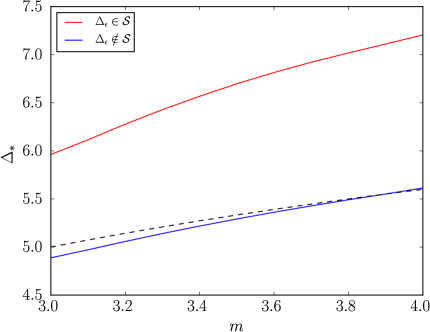
Refer to caption
Figure 5: Dimension bounds for irrelevant operators in (4.2). The dotted line shows the dimension of the primary scalar ϕ1,5subscriptitalic-ϕ15\phi_{1,5} whose multiplet needs to be replaced for 3<m<43𝑚43<m<4.

Checking the solvability of (4.1) for real λϵϵ𝒪subscript𝜆italic-ϵitalic-ϵ𝒪\lambda_{\epsilon\epsilon\mathcal{O}} is the simplest numerical bootstrap problem. Emphasizing the contributions of operators that are already present, we may write

𝒪λϵϵ𝒪2F,𝒪ϵϵ;ϵϵ(u,v)=F1,1(u,v)C(1,3)(1,3)(1,3)F1,3(u,v)subscript𝒪subscriptsuperscript𝜆2italic-ϵitalic-ϵ𝒪subscriptsuperscript𝐹italic-ϵitalic-ϵitalic-ϵitalic-ϵ𝒪𝑢𝑣subscript𝐹11𝑢𝑣subscriptsuperscript𝐶131313subscript𝐹13𝑢𝑣\displaystyle\sum_{\mathcal{O}}\lambda^{2}_{\epsilon\epsilon\mathcal{O}}F^{\epsilon\epsilon;\epsilon\epsilon}_{-,\mathcal{O}}(u,v)=-F_{1,1}(u,v)-C^{(1,3)}_{(1,3)(1,3)}F_{1,3}(u,v)
F1,1(u,v)n,n¯cnϵϵ(1,1)ϵϵcn¯ϵϵ(1,1)ϵϵF,n+n¯,|nn¯|ϵϵ;ϵϵ(u,v)subscript𝐹11𝑢𝑣subscript𝑛¯𝑛subscriptsuperscript𝑐italic-ϵitalic-ϵ11italic-ϵitalic-ϵ𝑛subscriptsuperscript𝑐italic-ϵitalic-ϵ11italic-ϵitalic-ϵ¯𝑛subscriptsuperscript𝐹italic-ϵitalic-ϵitalic-ϵitalic-ϵ𝑛¯𝑛𝑛¯𝑛𝑢𝑣\displaystyle F_{1,1}(u,v)\equiv\sum_{n,\bar{n}}c^{\epsilon\epsilon(1,1)\epsilon\epsilon}_{n}c^{\epsilon\epsilon(1,1)\epsilon\epsilon}_{\bar{n}}F^{\epsilon\epsilon;\epsilon\epsilon}_{-,n+\bar{n},|n-\bar{n}|}(u,v)
F1,3(u,v)n,n¯cnϵϵ(1,3)ϵϵcn¯ϵϵ(1,3)ϵϵF,Δϵ+n+n¯,|nn¯|ϵϵ;ϵϵ(u,v).subscript𝐹13𝑢𝑣subscript𝑛¯𝑛subscriptsuperscript𝑐italic-ϵitalic-ϵ13italic-ϵitalic-ϵ𝑛subscriptsuperscript𝑐italic-ϵitalic-ϵ13italic-ϵitalic-ϵ¯𝑛subscriptsuperscript𝐹italic-ϵitalic-ϵitalic-ϵitalic-ϵsubscriptΔitalic-ϵ𝑛¯𝑛𝑛¯𝑛𝑢𝑣\displaystyle F_{1,3}(u,v)\equiv\sum_{n,\bar{n}}c^{\epsilon\epsilon(1,3)\epsilon\epsilon}_{n}c^{\epsilon\epsilon(1,3)\epsilon\epsilon}_{\bar{n}}F^{\epsilon\epsilon;\epsilon\epsilon}_{-,\Delta_{\epsilon}+n+\bar{n},|n-\bar{n}|}(u,v)\;. (4.2)

Keeping operators with Δ30Δ30\Delta\leq 30, we have used the results of the last section to approximate the right-hand side of (4.2). In the sum over operators, there will be a continuum of irrelevant scalars not in ϕ1,1ϕ1,3subscriptitalic-ϕ11subscriptitalic-ϕ13\phi_{1,1}\cup\phi_{1,3} which begins at some gap Δ>2subscriptΔ2\Delta_{*}>2. If this is the only set of scalars on the left-hand side of (4.2), we are dealing with the set 𝒮={Δ>Δ}𝒮ΔsubscriptΔ\mathcal{S}=\{\Delta>\Delta_{*}\}. Alternatively, we could allow the dimension ΔϵsubscriptΔitalic-ϵ\Delta_{\epsilon} to appear again and enlarge it to 𝒮={Δ>Δ}{Δ=Δϵ}𝒮ΔsubscriptΔΔsubscriptΔitalic-ϵ\mathcal{S}=\{\Delta>\Delta_{*}\}\cup\{\Delta=\Delta_{\epsilon}\}. The second choice is the one applicable to Figure 1. However, in Figure 5, we consider the first choice as well. This is because it is possible to rederive Figure 1 under the requirement that ϵitalic-ϵ\epsilon is non-degenerate [16]. As numerical accuracy is improved, we expect the blue line to precisely meet the dotted line at m=4𝑚4m=4.171717Varying the spatial dimension provides one indication that numerical errors have a large effect. Evaluating conformal blocks at d=2.01𝑑2.01d=2.01 instead of d=2𝑑2d=2 results in a much smaller bound on ΔsubscriptΔ\Delta_{*}.

In Figure 5, the red curve tells us that (1.4) is admissible whenever we treat (Δσ,Δϵ)subscriptΔ𝜎subscriptΔitalic-ϵ(\Delta_{\sigma},\Delta_{\epsilon}) as allowed dimensions and perform a two-parameter scan. The blue curve tells us that (1.4) will still be admissible when we fix ϵitalic-ϵ\epsilon as a single operator at angle θ=arctan(λσσϵλϵϵϵ)𝜃arctansubscript𝜆𝜎𝜎italic-ϵsubscript𝜆italic-ϵitalic-ϵitalic-ϵ\theta=\mathrm{arctan}\left(\frac{\lambda_{\sigma\sigma\epsilon}}{\lambda_{\epsilon\epsilon\epsilon}}\right) and scan over (Δσ,Δϵ,θ)subscriptΔ𝜎subscriptΔitalic-ϵ𝜃(\Delta_{\sigma},\Delta_{\epsilon},\theta). Finally, one may contemplate the effect of imposing θ=π2𝜃𝜋2\theta=\frac{\pi}{2} which is one consequence of Kramers-Wannier duality in the Ising model. Although this question cannot be answered with Figure 5, we have found that (1.4) persists yet again. In all three cases, (1.4) is not just an allowed line — it is the maximal allowed line. From this, we must conclude that many solutions to crossing, labelled by values of ΔsubscriptΔ\Delta_{*} between the red and blue lines, lie along the bound on the left side of Figure 1. This signals the presence of a flat direction, e.g. a bound in (Δσ,Δϵ,θ)subscriptΔ𝜎subscriptΔitalic-ϵ𝜃(\Delta_{\sigma},\Delta_{\epsilon},\theta) space which is independent of θ𝜃\theta. A flat direction in the modular bootstrap was previously seen in [59]. The main argument for unique extremal functionals comes from [46], in which the multi-correlator bootstrap equations were augmented with angles for each operator in OPE space. To extract a spectrum in this formulation, one would have to look for zeros of these functionals on the entire (Δ,θ)Δ𝜃(\Delta,\theta) plane. We suspect that the flat direction here corresponds to a zero being achieved on a codimension-one locus.
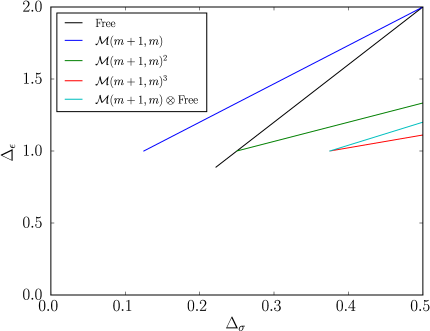
Refer to caption
Figure 6: Tensor product theories that are allowed in both sides of Figure 1. Since we must have Δϵ1subscriptΔitalic-ϵ1\Delta_{\epsilon}\geq 1, all other tensor products involving the free field vertex operators necessarily lie to the right.

Because the generalized minimal model line (1.4) is allowed by the bootstrap, there are several lines in the interior of Figure 1 that must be allowed as well. These can be constructed through one or more tensor products. If we multiply two generalized minimal models for instance, the only non-trivial operator whose dimension lies to the left of Δσ=12subscriptΔ𝜎12\Delta_{\sigma}=\frac{1}{2} is σσtensor-product𝜎𝜎\sigma\otimes\sigma. Writing its OPE schematically,

(σσ)×(σσ)=(II)+(Iϵ)+(ϵI)+(ϵϵ)+tensor-product𝜎𝜎tensor-product𝜎𝜎tensor-product𝐼𝐼tensor-product𝐼italic-ϵtensor-productitalic-ϵ𝐼tensor-productitalic-ϵitalic-ϵ(\sigma\otimes\sigma)\times(\sigma\otimes\sigma)=(I\otimes I)+(I\otimes\epsilon)+(\epsilon\otimes I)+(\epsilon\otimes\epsilon)+\dots (4.3)

includes two relevant operators. In order for these to have the same scaling dimension, the (m+1,m)(m+1,m)tensor-product𝑚1𝑚superscript𝑚1superscript𝑚\mathcal{M}(m+1,m)\otimes\mathcal{M}(m^{\prime}+1,m^{\prime}) product must have m=m𝑚superscript𝑚m=m^{\prime}. Expanding the search to include free theories and generalized free theories, it is a simple exercise to check that the lines in Figure 6 all have one relevant 2subscript2\mathbb{Z}_{2}-odd scaling dimension and one relevant 2subscript2\mathbb{Z}_{2}-even scaling dimension.

Evidently, it is not possible to isolate particular minimal models in a three-correlator bootstrap by specifying the number of relevant operators. One has to consider more stringent assumptions or add more correlators. The former approach was discussed already in [60], where it was found that the one-correlator Ising kink sharpens considerably when scalars are restricted to lie in 𝒮={Δ>3}{Δ=Δϵ}𝒮Δ3ΔsubscriptΔitalic-ϵ\mathcal{S}=\{\Delta>3\}\cup\{\Delta=\Delta_{\epsilon}\}. This kink becomes an island when a similar restriction is made for a three-correlator system. Following [61], it is likely that one can obtain this island from a single correlator by imposing large gaps in the spin-0 and spin-2 sectors.

Coefficients Signs
C(1,4)(1,4)(1,3)subscriptsuperscript𝐶131414C^{(1,3)}_{(1,4)(1,4)} Positive
C(1,4)(1,4)(1,5)subscriptsuperscript𝐶151414C^{(1,5)}_{(1,4)(1,4)} Negative for m<4𝑚4m<4
C(1,4)(1,4)(1,7)subscriptsuperscript𝐶171414C^{(1,7)}_{(1,4)(1,4)} Negative for m<6𝑚6m<6
C(1,3)(1,4)(1,6)subscriptsuperscript𝐶161314C^{(1,6)}_{(1,3)(1,4)} Negative for m<5𝑚5m<5
C(1,2)(1,4)(1,5)subscriptsuperscript𝐶151214C^{(1,5)}_{(1,2)(1,4)} Negative for m<4𝑚4m<4
Table 6: Virasoro block coefficients (other than the ones in Figure 4) appearing in four-point functions made from σ𝜎\sigma, ϵitalic-ϵ\epsilon and σsuperscript𝜎\sigma^{\prime}. Only one is non-negative for all m3𝑚3m\geq 3.

A more ambitious goal is to produce islands under minimal assumptions by introducing a third external scalar. Taking this external scalar to be odd, plots along the lines of Figure 4 offer some preliminary insight.181818The lightest 2subscript2\mathbb{Z}_{2}-odd scalar after σ𝜎\sigma is σϕ1,4superscript𝜎subscriptitalic-ϕ14\sigma^{\prime}\equiv\phi_{1,4}. The lightest 2subscript2\mathbb{Z}_{2}-even scalar after ϵitalic-ϵ\epsilon is ϵ[L2L¯2,ϕ1,1]superscriptitalic-ϵsubscript𝐿2subscript¯𝐿2subscriptitalic-ϕ11\epsilon^{\prime}\equiv[L_{-2}\bar{L}_{-2},\phi_{1,1}]. We have made the choice in which all operator fusions are between Virasoro primaries. Regions where all C(r1,s1)(r2,s2)(r3,s3)>0superscriptsubscript𝐶subscript𝑟1subscript𝑠1subscript𝑟2subscript𝑠2subscript𝑟3subscript𝑠30C_{(r_{1},s_{1})(r_{2},s_{2})}^{(r_{3},s_{3})}>0 are likely to survive, but as Table 6 shows, there can be several negative structure constants with more than three correlators. We have seen that the negative constant C(1,3)(1,3)(1,5)subscriptsuperscript𝐶151313C^{(1,5)}_{(1,3)(1,3)} in the three-correlator system was innocuous because it did not appear in any mixed correlators. It is therefore encouraging that the coefficients C(1,2)(1,4)(1,5)subscriptsuperscript𝐶151214C^{(1,5)}_{(1,2)(1,4)} and C(1,3)(1,4)(1,6)subscriptsuperscript𝐶161314C^{(1,6)}_{(1,3)(1,4)}, which have first-order zeros, participate in σσσσdelimited-⟨⟩𝜎𝜎superscript𝜎superscript𝜎\left<\sigma\sigma\sigma^{\prime}\sigma^{\prime}\right> and ϵϵσσdelimited-⟨⟩italic-ϵitalic-ϵsuperscript𝜎superscript𝜎\left<\epsilon\epsilon\sigma^{\prime}\sigma^{\prime}\right> respectively. Lest we become too encouraged, it is important to note that ΔσsubscriptΔsuperscript𝜎\Delta_{\sigma^{\prime}} is defined as the starting point for a continuum of irrelevant operators. This represents a fundamental difference as compared to the one-correlator and three-correlator analysis. It remains to be seen whether we can still derive strong bounds from a scan over two isolated scaling dimensions and one non-isolated scaling dimension.

4.2 Conformal manifolds

Even though the tensor product lines above all have Δσ>14subscriptΔ𝜎14\Delta_{\sigma}>\frac{1}{4}, there could be other CFTs in 18<Δσ<1518subscriptΔ𝜎15\frac{1}{8}<\Delta_{\sigma}<\frac{1}{5} with sufficiently few relevant operators to survive the constraints of σ𝜎\sigma, ϵitalic-ϵ\epsilon and σsuperscript𝜎\sigma^{\prime}. An interesting possibility, that would complicate the search for islands, is a continuous line of theories ending somewhere close to the Ising model. We may search for an example by using the extremal functional method on solutions to crossing that involve a scalar ΦΦ\Phi of dimension 2.191919The idea of building up a previously unknown conformal manifold was discussed in [62]. Their method uses large-N𝑁N perturbation theory to construct the holographic dual of a bulk action with shift-symmetric couplings. For a recent bootstrap study of a known conformal manifold, see [63]. This provides another opportunity to predict a mixed correlator result without actually bootstrapping more than one correlator.

The first step is to maximize λσσΦ2subscriptsuperscript𝜆2𝜎𝜎Φ\lambda^{2}_{\sigma\sigma\Phi} in the range 18<Δσ<1218subscriptΔ𝜎12\frac{1}{8}<\Delta_{\sigma}<\frac{1}{2} with the constraint that all scalar dimensions are above 2Δσ2subscriptΔ𝜎2\Delta_{\sigma}. Each point saturating the bound yields a spectrum with the marginal deformation ΦΦ\Phi. To see that this set of solutions is not a conformal manifold, we may check that the central charge varies with ΔσsubscriptΔ𝜎\Delta_{\sigma}. Specifically, it reaches a minimum value of c1.12𝑐1.12c\approx 1.12. It is then straightforward to force our putative theories to have this central charge (or any larger value) by taking

F,0,0σσ;σσ(u,v)F,0,0σσ;σσ(u,v)+Δσ2cF,2,2σσ;σσ(u,v)maps-tosubscriptsuperscript𝐹𝜎𝜎𝜎𝜎00𝑢𝑣subscriptsuperscript𝐹𝜎𝜎𝜎𝜎00𝑢𝑣superscriptsubscriptΔ𝜎2𝑐subscriptsuperscript𝐹𝜎𝜎𝜎𝜎22𝑢𝑣F^{\sigma\sigma;\sigma\sigma}_{-,0,0}(u,v)\mapsto F^{\sigma\sigma;\sigma\sigma}_{-,0,0}(u,v)+\frac{\Delta_{\sigma}^{2}}{c}F^{\sigma\sigma;\sigma\sigma}_{-,2,2}(u,v) (4.4)

in the usual one-correlator crossing equation. To prevent (4.4) from being undone by a second copy of the stress tensor, we have imposed the gap ΔT>2.1subscriptΔ𝑇2.1\Delta_{T}>2.1 on spin-2 operators. Performing a second pass in this way, we have found low-lying dimensions and OPE coefficients with examples plotted in Figure 7. With constant c𝑐c and ΔΦsubscriptΔΦ\Delta_{\Phi}, these CFT data appear to satisfy all constraints of a conformal manifold that are directly accessible to σσσσdelimited-⟨⟩𝜎𝜎𝜎𝜎\left<\sigma\sigma\sigma\sigma\right>. Despite this, there is a method from [29] that can be revived to gain indirect information about the next four-point function, which we will call ϵϵϵϵdelimited-⟨⟩italic-ϵitalic-ϵitalic-ϵitalic-ϵ\left<\epsilon\epsilon\epsilon\epsilon\right>.

Refer to caption
(a)
Refer to caption
(b)
Figure 7: Dimensions and OPE coefficients for scalars in the spectrum maximizing λσσΦ2subscriptsuperscript𝜆2𝜎𝜎Φ\lambda^{2}_{\sigma\sigma\Phi}. The green and blue lines are ϵitalic-ϵ\epsilon and ΦΦ\Phi respectively.

The key is that the dimensions in σ×σ𝜎𝜎\sigma\times\sigma are also the dimensions in any OPE between identical scalars. Given a sufficiently long list of scaling dimensions, there is no reason why a search for optimal OPE coefficients has to be done for σ×σ𝜎𝜎\sigma\times\sigma rather than ϵ×ϵitalic-ϵitalic-ϵ\epsilon\times\epsilon. We confirm this in Appendix B, by taking an approximate Ising model spectrum and performing the same type of fit that was done in [29]. Our results show that the estimation of λσσ𝒪2subscriptsuperscript𝜆2𝜎𝜎𝒪\lambda^{2}_{\sigma\sigma\mathcal{O}} could have been extended to λϵϵ𝒪2subscriptsuperscript𝜆2italic-ϵitalic-ϵ𝒪\lambda^{2}_{\epsilon\epsilon\mathcal{O}} without the three-correlator crossing equations. The fitting procedure therefore differs from the primal method of [45], which is more accurate but limited to the direct correlators under study. Assuming that the method can be trusted, at least for 2D theories, we now have access to ϵ×ϵitalic-ϵitalic-ϵ\epsilon\times\epsilon coefficients including λϵϵΦsubscript𝜆italic-ϵitalic-ϵΦ\lambda_{\epsilon\epsilon\Phi}. This allows another property of conformal manifolds to be tested.
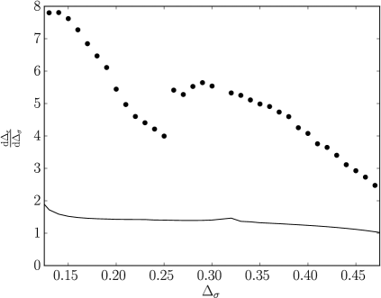
Refer to caption
Figure 8: The slope of ΔϵsubscriptΔitalic-ϵ\Delta_{\epsilon} as one goes through the artificial spectra parameterized by ΔσsubscriptΔ𝜎\Delta_{\sigma}. The points, predicted by (4.5), would have to match if these operators were to come from a genuine theory with a dimensionless coupling.

When CFTs are parameterized by an exactly marginal operator with coupling g𝑔g, there is a complicated set of differential equations that their local data must satisfy [64, 65]. The simplest of these is dΔidg=Sd1λiiΦdsubscriptΔ𝑖d𝑔subscript𝑆𝑑1subscript𝜆𝑖𝑖Φ\frac{\textup{d}\Delta_{i}}{\textup{d}g}=-S_{d-1}\lambda_{ii\Phi} which reads dΔidg=2πλiiΦdsubscriptΔ𝑖d𝑔2𝜋subscript𝜆𝑖𝑖Φ\frac{\textup{d}\Delta_{i}}{\textup{d}g}=-2\pi\lambda_{ii\Phi} in two dimensions. The constraint

dΔϵdΔσ=λϵϵΦλσσΦdsubscriptΔitalic-ϵdsubscriptΔ𝜎subscript𝜆italic-ϵitalic-ϵΦsubscript𝜆𝜎𝜎Φ\frac{\textup{d}\Delta_{\epsilon}}{\textup{d}\Delta_{\sigma}}=\frac{\lambda_{\epsilon\epsilon\Phi}}{\lambda_{\sigma\sigma\Phi}} (4.5)

immediately follows. The two sides of this equation have been plotted in Figure 8. Even though λϵϵΦsubscript𝜆italic-ϵitalic-ϵΦ\lambda_{\epsilon\epsilon\Phi} is not known with high precision, the noise in the data seems much too small to explain the violation of (4.5). We must conclude that if a conformal manifold in 18<Δσ<1218subscriptΔ𝜎12\frac{1}{8}<\Delta_{\sigma}<\frac{1}{2} allowed by Figure 1 exists, it is not privileged enough to be found by this one-correlator exercise.

It would be very interesting to find other applications for the dual method in [29]. Unfortunately, Appendix B shows that results become much less reliable above d=2𝑑2d=2. A possible reason for this was given in [47] which noticed a surprising preference for double-twist operators in the 3D numerical bootstrap. To review, double-twist families have the following schematic form for \ell\rightarrow\infty:

[ϕϕ]nsubscriptdelimited-[]italic-ϕitalic-ϕ𝑛\displaystyle[\phi\phi]_{n} =\displaystyle= ϕμ1μnϕitalic-ϕsuperscriptsubscript𝜇1superscriptsubscript𝜇superscript𝑛italic-ϕ\displaystyle\phi\partial^{\mu_{1}}\dots\partial^{\mu_{\ell}}\Box^{n}\phi
τ𝜏\displaystyle\tau =\displaystyle= 2τϕ+2n+O(1).2subscript𝜏italic-ϕ2𝑛𝑂superscript1\displaystyle 2\tau_{\phi}+2n+O(\ell^{-1})\;. (4.6)

The lightcone bootstrap requires them to appear in any CFT with a twist gap [66, 67]. When d>2𝑑2d>2, every operator except the identity has positive twist and the extremal functional method is able to find spectra dominated by (4.6). The absence of other operators interferes with our ability to fit OPE coefficients. Convsersely, 2D theories have no need for double-twist operators as the identity, stress tensor and higher-spin currents all have τ=0𝜏0\tau=0. The quality of our fit suggests that this resolves the main source of bias in the extremal spectrum.

4.3 Supersymmetric minimal models

So far, we have been concerned with finding the necessary correlators to single out theories that are minimal with respect to the Virasoro algebra. However, the unitary representations of the 𝒩=1𝒩1\mathcal{N}=1 super-Virasoro algebra also admit a discrete series for central charges below that of the free field. In analogy with (m+1,m)𝑚1𝑚\mathcal{M}(m+1,m), we can continue them to 𝒮(m+2,m)𝒮𝑚2𝑚\mathcal{SM}(m+2,m) where non-integer m𝑚m breaks unitarity but preserves crossing symmetry. Studying these solved theories offers another route toward understanding the systematics of the bootstrap. It could also be interesting to compare results for the tricritical Ising model since this is the lowest model of 𝒮(m+2,m)𝒮𝑚2𝑚\mathcal{SM}(m+2,m) but the second lowest model of (m+1,m)𝑚1𝑚\mathcal{M}(m+1,m).

The super-Virasoro graded commutation relations

[Lm,Ln]subscript𝐿𝑚subscript𝐿𝑛\displaystyle\left[L_{m},L_{n}\right] =\displaystyle= (mn)Lm+n+c12m(m1)(m+1)δm+n,0𝑚𝑛subscript𝐿𝑚𝑛𝑐12𝑚𝑚1𝑚1subscript𝛿𝑚𝑛0\displaystyle(m-n)L_{m+n}+\frac{c}{12}m(m-1)(m+1)\delta_{m+n,0}
[Lm,Gr]subscript𝐿𝑚subscript𝐺𝑟\displaystyle\left[L_{m},G_{r}\right] =\displaystyle= (m2r)Gm+r𝑚2𝑟subscript𝐺𝑚𝑟\displaystyle\left(\frac{m}{2}-r\right)G_{m+r}
{Gr,Gs}subscript𝐺𝑟subscript𝐺𝑠\displaystyle\{G_{r},G_{s}\} =\displaystyle= 2Lr+s+c3(r12)(r+12)δr+s,02subscript𝐿𝑟𝑠𝑐3𝑟12𝑟12subscript𝛿𝑟𝑠0\displaystyle 2L_{r+s}+\frac{c}{3}\left(r-\frac{1}{2}\right)\left(r+\frac{1}{2}\right)\delta_{r+s,0} (4.7)

actually describe two algebras since fermions do not have to be periodic in radial quantization. When the indices on Grsubscript𝐺𝑟G_{r} are integers, (4.7) is the Ramond superalgebra, otherwise it is the Neveu-Schwarz superalgebra. The super-Virasoro minimal models, which contain representations of each, have a Kac formula given by

c𝑐\displaystyle c =\displaystyle= 3212m(m+2)m>23212𝑚𝑚2𝑚2\displaystyle\frac{3}{2}-\frac{12}{m(m+2)}\;\;\;\;\;\;\;\;\;\;\;\;\;\;\;\;\;\;\;\;\;\;\;\;\;\;\;\;\;\;\;\;\;\;\;\;\;\;\;\;\;\;m>2
hr,ssubscript𝑟𝑠\displaystyle h_{r,s} =\displaystyle= [(m+2)rms]248m(m+2)+132[1(1)rs]r,s>0.superscriptdelimited-[]𝑚2𝑟𝑚𝑠248𝑚𝑚2132delimited-[]1superscript1𝑟𝑠𝑟𝑠subscriptabsent0\displaystyle\frac{[(m+2)r-ms]^{2}-4}{8m(m+2)}+\frac{1}{32}[1-(-1)^{r-s}]\;\;\;r,s\in\mathbb{Z}_{>0}\;. (4.8)

If rs𝑟𝑠r-s is even (odd), this is a Neveu-Schwarz (Ramond) degenerate weight [68]. In either case, it is degenerate at level rs/2𝑟𝑠2rs/2. It is clear by inspection that G±12subscript𝐺plus-or-minus12G_{\pm\frac{1}{2}} generate a subalgebra of (4.7) that is independent of c𝑐c. For integer indices, on the other hand, no global subalgebra exists. A numerical bootstrap approach is therefore most readily accessible for the Neveu-Schwarz sectors of 𝒩=(1,1)𝒩11\mathcal{N}=(1,1) theories.

In the global algebra, which is 𝔬𝔰𝔭(2|1)𝔬𝔰𝔭conditional21\mathfrak{osp}(2|1), primary operators may be written as superfields; Φ(z,θ)=ϕ(z)+θψ(z)Φ𝑧𝜃italic-ϕ𝑧𝜃𝜓𝑧\Phi(z,\theta)=\phi(z)+\theta\psi(z). The superspace distance, which enters in correlation functions, is Zijzizjθiθjsubscript𝑍𝑖𝑗subscript𝑧𝑖subscript𝑧𝑗subscript𝜃𝑖subscript𝜃𝑗Z_{ij}\equiv z_{i}-z_{j}-\theta_{i}\theta_{j}. Even though cross-ratios in dsuperscript𝑑\mathbb{R}^{d} all involve at least four points, invariant combinations in superspace may be built using three points as well. The quantity

η=θ1Z23+θ2Z31+θ3Z12+θ1θ2θ3Z12Z23Z31𝜂subscript𝜃1subscript𝑍23subscript𝜃2subscript𝑍31subscript𝜃3subscript𝑍12subscript𝜃1subscript𝜃2subscript𝜃3subscript𝑍12subscript𝑍23subscript𝑍31\eta=\frac{\theta_{1}Z_{23}+\theta_{2}Z_{31}+\theta_{3}Z_{12}+\theta_{1}\theta_{2}\theta_{3}}{\sqrt{Z_{12}Z_{23}Z_{31}}} (4.9)

is invariant under 𝔬𝔰𝔭(2|1)𝔬𝔰𝔭conditional21\mathfrak{osp}(2|1) [69]. As a result, the three-point function depends on more than just an OPE coefficient. The general expression for the chiral half is

Φ1(z1,θ1)Φ2(z2,θ2)Φ3(z3,θ3)=λ123(1+ζη)Z12h1+h2h3Z23h2+h3h1Z31h3+h1h2delimited-⟨⟩subscriptΦ1subscript𝑧1subscript𝜃1subscriptΦ2subscript𝑧2subscript𝜃2subscriptΦ3subscript𝑧3subscript𝜃3subscript𝜆1231𝜁𝜂superscriptsubscript𝑍12subscript1subscript2subscript3superscriptsubscript𝑍23subscript2subscript3subscript1superscriptsubscript𝑍31subscript3subscript1subscript2\left<\Phi_{1}(z_{1},\theta_{1})\Phi_{2}(z_{2},\theta_{2})\Phi_{3}(z_{3},\theta_{3})\right>=\frac{\lambda_{123}(1+\zeta\eta)}{Z_{12}^{h_{1}+h_{2}-h_{3}}Z_{23}^{h_{2}+h_{3}-h_{1}}Z_{31}^{h_{3}+h_{1}-h_{2}}} (4.10)

where ζ𝜁\zeta is an arbitrary Grassman number. Until recently, such extra parameters were eliminated by restricting the superconformal bootstrap to correlators of BPS operators [12, 13]. We may indeed impose shortening conditions on (4.10), but due to the small amount of supersymmetry, this would require us to give up a lot. To be annihilated by a supercharge, each external operator would have to be the identity in at least one of the 𝔬𝔰𝔭(2|1)𝔬𝔰𝔭conditional21\mathfrak{osp}(2|1) factors. It is therefore preferable to leave (4.10) in its most general form and use superconformal blocks that include unknown coefficients reflecting the presence of ζ𝜁\zeta.

The authors of [54] computed some of the necessary blocks and introduced a framework that still allows the bootstrap to proceed. Their idea is to consider an entire multiplet at once, with the external correlators involving all combinations of a primary and its super-descendants. When this is carried out for 𝒩=(1,1)𝒩11\mathcal{N}=(1,1), the allowed regions will have to include all points corresponding to the 𝒮(m+2,m)𝒮𝑚2𝑚\mathcal{SM}(m+2,m). The strongest statement we can make from this is that the line

Δϵ=83ΔσsubscriptΔitalic-ϵ83subscriptΔ𝜎\Delta_{\epsilon}=\frac{8}{3}\Delta_{\sigma} (4.11)

must be inside the bound for Δσ<18subscriptΔ𝜎18\Delta_{\sigma}<\frac{1}{8}. This comes from choosing the Neveu-Schwarz fields σϕ2,2𝜎subscriptitalic-ϕ22\sigma\equiv\phi_{2,2} and ϵϕ3,3italic-ϵsubscriptitalic-ϕ33\epsilon\equiv\phi_{3,3}. Right at Δσ=18subscriptΔ𝜎18\Delta_{\sigma}=\frac{1}{8}, we find ourselves in the c=1𝑐1c=1 model where ϕ3,3=ϕ1,3subscriptitalic-ϕ33subscriptitalic-ϕ13\phi_{3,3}=\phi_{1,3} and the entire level-3232\frac{3}{2} subspace decouples. To see this, we may check that

|χ=[G3222h+1L1G12]|hket𝜒delimited-[]subscript𝐺32221subscript𝐿1subscript𝐺12ket\left|\chi\right>=\left[G_{-\frac{3}{2}}-\frac{2}{2h+1}L_{-1}G_{-\frac{1}{2}}\right]\left|h\right> (4.12)

is the unique quasiprimary state. Computing the norm and setting hh3,3maps-tosubscript33h\mapsto h_{3,3}, we find

χ|χinner-product𝜒𝜒\displaystyle\left<\chi|\chi\right> =\displaystyle= 2(2ch+c+6h29h)3(2h+1)22𝑐𝑐6superscript29321\displaystyle\frac{2(2ch+c+6h^{2}-9h)}{3(2h+1)} (4.13)
maps-to\displaystyle\mapsto (m4)(m+6)m2+2m+8𝑚4𝑚6superscript𝑚22𝑚8\displaystyle\frac{(m-4)(m+6)}{m^{2}+2m+8}

with a first-order zero. This is the behaviour that we saw for m=3𝑚3m=3 in the bosonic case, but now it occurs for m=4𝑚4m=4. The tricritical Ising model, which has no ϕ3,3subscriptitalic-ϕ33\phi_{3,3} operator, lives at the point (Δσ,Δϵ)=(110,110)subscriptΔ𝜎subscriptΔitalic-ϵ110110(\Delta_{\sigma},\Delta_{\epsilon})=\left(\frac{1}{10},\frac{1}{10}\right).

The above calculation shows that a global block coefficient in the supersymmetric generalized minimal model line becomes negative for m<4𝑚4m<4. If we are to see an associated kink, this line must saturate the bound on operator dimensions from the long multiplet bootstrap. This brings us to a crucial difference between (m+1,m)𝑚1𝑚\mathcal{M}(m+1,m) and the Neveu-Schwarz sector of 𝒮(m+2,m)𝒮𝑚2𝑚\mathcal{SM}(m+2,m). In the former case, we saw the correct saturation with (1.4). The same cannot hold for (4.11) because it is strictly below the line for vertex operators. Writing a CFT vertex operator as eiqϕ(z)superscript𝑒𝑖𝑞italic-ϕ𝑧e^{iq\phi(z)} and an SCFT vertex operator as eiqΦ(z,θ)superscript𝑒𝑖𝑞Φ𝑧𝜃e^{iq\Phi(z,\theta)}, the two important properties are Δq2proportional-toΔsuperscript𝑞2\Delta\propto q^{2} and additivity of q𝑞q. These lead to Δϵ=4ΔσsubscriptΔitalic-ϵ4subscriptΔ𝜎\Delta_{\epsilon}=4\Delta_{\sigma} which is allowed by the one-correlator region of Figure 1. Due to the restriction on the number of relevant operators, the three-correlator region omits this line until Δσ=29subscriptΔ𝜎29\Delta_{\sigma}=\frac{2}{9}. It is therefore clear that treating four copies of the same multiplet with the methods of [54] is not enough. If our goal is to see a minimal model kink, the 𝒩=(1,1)𝒩11\mathcal{N}=(1,1) bootstrap will require multiple correlators at the superspace level. Since each of these must separately expand to a mixed correlator system, the resulting problem is likely to be numerically intensive.

5 Conclusion

Through a combination of analytic techniques and one-correlator numerics, we have explained an important aspect of Figure 1 — we have shown that the constraints on four-point functions of relevant operators are not strong enough to exclude the generalized minimal models. Constraints that are strong enough may be used in the conformal or superconformal bootstrap, but only when the number of four-point functions exceeds the maximum system size that has been tested to date.

Our analysis proceeded correlator-by-correlator. For σσσσdelimited-⟨⟩𝜎𝜎𝜎𝜎\left<\sigma\sigma\sigma\sigma\right>, the results were exact. The expressions (3.21) and (3.26) ensured that the global block coefficients involved were all positive. For σσϵϵdelimited-⟨⟩𝜎𝜎italic-ϵitalic-ϵ\left<\sigma\sigma\epsilon\epsilon\right>, all but one coefficient appeared to be positive upon using the approach of [17] — we simply expanded in 𝔰𝔩(2)𝔰𝔩2\mathfrak{sl}(2) blocks to high order and conjectured that the pattern continues to hold. For ϵϵϵϵdelimited-⟨⟩italic-ϵitalic-ϵitalic-ϵitalic-ϵ\left<\epsilon\epsilon\epsilon\epsilon\right>, two pieces of the (m+1,m)𝑚1𝑚\mathcal{M}(m+1,m) line had to be treated separately. In 4<m<4𝑚4<m<\infty, it was enough to compute coefficients again and see that there were no obvious signs of unitarity violation. However, 3<m<43𝑚43<m<4 required an exotic solution having only partial overlap with the CFT data of a generalized minimal model. It was possible to see evidence of this in the one-correlator bootstrap because of a special property of ϕ1,5subscriptitalic-ϕ15\phi_{1,5} operators, namely their absence from the superselection sector σ×σ𝜎𝜎\sigma\times\sigma. This had interesting implications for the uniqueness results in [46].

A possible future endeavour is to put all correlators on the same footing as σσσσdelimited-⟨⟩𝜎𝜎𝜎𝜎\left<\sigma\sigma\sigma\sigma\right>. In order to do this, one does not necessarily have to solve for c2nϵϵ(1,s)ϵϵsubscriptsuperscript𝑐italic-ϵitalic-ϵ1𝑠italic-ϵitalic-ϵ2𝑛c^{\epsilon\epsilon(1,s)\epsilon\epsilon}_{2n} as a known special function. The c2nσσ(1,s)σσsubscriptsuperscript𝑐𝜎𝜎1𝑠𝜎𝜎2𝑛c^{\sigma\sigma(1,s)\sigma\sigma}_{2n} were ultimately shown to be positive using only the recursion for Wilson polynomials. Instead, the main challenge in extending the positivity proof is expressing global block coefficients as solutions of one recurrence relation instead of two. Our current approach, based on the BPZ equation, is awkward in this respect. It uses the Frobenius method to evaluate Taylor coefficients and then feeds these into a second recursion to obtain global block coefficients. It is worth checking if hypergeometric identities can be used to derive a recursion that operates on global block coefficients directly. It would also be interesting to take a closer look at super-BPZ equations. Our discussion surrounding the vanishing norm (4.13) can be made more systematic if we also check how other 𝔬𝔰𝔭(2|1)𝔬𝔰𝔭conditional21\mathfrak{osp}(2|1) blocks appear. BPZ differential equations in superspace have been studied in [68, 69] and some of them are second-order. This is exactly what we need to go beyond recurrence relations and apply the decompositions in [21, 22]. Additionally, these methods could be applicable to the KZ equations associated with extended chiral algebras. A realistic hope is using them to explain a numerical bound in [70] which interpolates between 𝒲3subscript𝒲3\mathcal{W}_{3}-minimal models.

The last possibility we have discussed is an extension of the extremal functional method — reviving the fit in [29] to estimate more OPE coefficients than the ones that are known to high precision. While we only used this to demonstrate a null result, it would be interesting to find a further use for it in two dimensions. Complications in higher dimensions arise due to the privileged role of double-twist operators in the numerical bootstrap; a result that is not fully understood [47]. One should be able to get a sense of how robust it is by studying alternative bootstrap algorithms such as the one in [71].

Acknowledgements

This work was partially supported by the Natural Sciences and Engineering Research Council of Canada. Numerical results in this paper were obtained using the high-performance computing system at the Institute for Advanced Computational Science at Stony Brook University. I am grateful for discussions with Shai Chester, Liam Fitzpatrick, Anton de la Fuente, Matthijs Hogvervorst, Jaehoon Lee, Madalena Lemos, Dalimil Mazáč, Miguel Paulos, Leonardo Rastelli, Slava Rychkov, David Simmons-Duffin, Balt van Rees and Alessandro Vichi. Most of these took place at various meetings of the Simons Collaboration on the Nonperturbative Bootstrap.

Appendix A Linear difference equations

We have regularly encountered linear recursions with three terms such as (2.13) and (3.29). Asymptotic analysis of sequences obeying these relations is a well understood subject, going by the name Birkhoff-Trjitzinsky theory. The following theorem summarizes a number of results from it [72].

Theorem 1.

Let y1(n)subscript𝑦1𝑛y_{1}(n) and y2(n)subscript𝑦2𝑛y_{2}(n) be the two linearly independent solutions of the difference equation

y(n+2)+a(n)y(n+1)+b(n)y(n)=0𝑦𝑛2𝑎𝑛𝑦𝑛1𝑏𝑛𝑦𝑛0y(n+2)+a(n)y(n+1)+b(n)y(n)=0 (A.1)

where the coefficients have asymptotic expansions a(n)s=0asnssimilar-to𝑎𝑛superscriptsubscript𝑠0subscript𝑎𝑠superscript𝑛𝑠a(n)\sim\sum_{s=0}^{\infty}\frac{a_{s}}{n^{s}} and b(n)s=0bsnssimilar-to𝑏𝑛superscriptsubscript𝑠0subscript𝑏𝑠superscript𝑛𝑠b(n)\sim\sum_{s=0}^{\infty}\frac{b_{s}}{n^{s}}.

  1. 1.

    If the characteristic equation ρ2+a0ρ+b0=0superscript𝜌2subscript𝑎0𝜌subscript𝑏00\rho^{2}+a_{0}\rho+b_{0}=0 has two distinct roots ρ1subscript𝜌1\rho_{1} and ρ2subscript𝜌2\rho_{2}, the solutions satisfy yj(n)ρjnnαjs=0cs,jnssimilar-tosubscript𝑦𝑗𝑛superscriptsubscript𝜌𝑗𝑛superscript𝑛subscript𝛼𝑗superscriptsubscript𝑠0subscript𝑐𝑠𝑗superscript𝑛𝑠y_{j}(n)\sim\rho_{j}^{n}n^{\alpha_{j}}\sum_{s=0}^{\infty}\frac{c_{s,j}}{n^{s}} where αj=a1ρj+b1a0ρj+2b0subscript𝛼𝑗subscript𝑎1subscript𝜌𝑗subscript𝑏1subscript𝑎0subscript𝜌𝑗2subscript𝑏0\alpha_{j}=\frac{a_{1}\rho_{j}+b_{1}}{a_{0}\rho_{j}+2b_{0}}.

  2. 2.

    Otherwise, consider the double root ρ𝜌\rho. If the auxiliary equation a1ρ+b1=0subscript𝑎1𝜌subscript𝑏10a_{1}\rho+b_{1}=0 is not satisfied, the solutions satisfy yj(n)ρne(1)jβnnαs=0(1)jscsns/2similar-tosubscript𝑦𝑗𝑛superscript𝜌𝑛superscript𝑒superscript1𝑗𝛽𝑛superscript𝑛𝛼superscriptsubscript𝑠0superscript1𝑗𝑠subscript𝑐𝑠superscript𝑛𝑠2y_{j}(n)\sim\rho^{n}e^{(-1)^{j}\beta\sqrt{n}}n^{\alpha}\sum_{s=0}^{\infty}(-1)^{js}\frac{c_{s}}{n^{s/2}} where α=14+b12b0𝛼14subscript𝑏12subscript𝑏0\alpha=\frac{1}{4}+\frac{b_{1}}{2b_{0}} and β=2a0a12b12b0𝛽2subscript𝑎0subscript𝑎12subscript𝑏12subscript𝑏0\beta=2\sqrt{\frac{a_{0}a_{1}-2b_{1}}{2b_{0}}}.

  3. 3.

    Otherwise, consider the roots α1subscript𝛼1\alpha_{1} and α2subscript𝛼2\alpha_{2} of the indicial equation α(α1)ρ2+(a1α+a2)ρ+b2=0𝛼𝛼1superscript𝜌2subscript𝑎1𝛼subscript𝑎2𝜌subscript𝑏20\alpha(\alpha-1)\rho^{2}+(a_{1}\alpha+a_{2})\rho+b_{2}=0, ordered according to α2α1subscript𝛼2subscript𝛼1\Re\alpha_{2}\geq\Re\alpha_{1}. If α2α10subscript𝛼2subscript𝛼1subscriptabsent0\alpha_{2}-\alpha_{1}\notin\mathbb{Z}_{\geq 0}, the solutions satisfy yj(n)ρnnαjs=0cs,jnssimilar-tosubscript𝑦𝑗𝑛superscript𝜌𝑛superscript𝑛subscript𝛼𝑗superscriptsubscript𝑠0subscript𝑐𝑠𝑗superscript𝑛𝑠y_{j}(n)\sim\rho^{n}n^{\alpha_{j}}\sum_{s=0}^{\infty}\frac{c_{s,j}}{n^{s}}.

  4. 4.

    Otherwise, let m=α2α1𝑚subscript𝛼2subscript𝛼1m=\alpha_{2}-\alpha_{1}. The asymptotic expansion for the first solution is unchanged from the previous case but for the second solution we must use y2(n)ρnnα2(s=0dsnsdmnm)+clog(n)y1(n)similar-tosubscript𝑦2𝑛superscript𝜌𝑛superscript𝑛subscript𝛼2superscriptsubscript𝑠0subscript𝑑𝑠superscript𝑛𝑠subscript𝑑𝑚superscript𝑛𝑚𝑐𝑛subscript𝑦1𝑛y_{2}(n)\sim\rho^{n}n^{\alpha_{2}}\left(\sum_{s=0}^{\infty}\frac{d_{s}}{n^{s}}-\frac{d_{m}}{n^{m}}\right)+c\log(n)y_{1}(n).

Taking (A.1) to be the recurrence relation for Wilson polynomials, we find the roots ρ=1𝜌1\rho=1, α1=2(a+x)subscript𝛼12𝑎𝑥\alpha_{1}=-2(a+x) and α2=2(ax)subscript𝛼22𝑎𝑥\alpha_{2}=-2(a-x) in the third case of the theorem. Each coefficient in (3.28) can then be written as a linear combination of two functions asymptotic to power laws. As seen in Table 7, all of them decay to zero. When comparing to the results of [73, 74], one must remember that c2nσσ(1,1)σσsubscriptsuperscript𝑐𝜎𝜎11𝜎𝜎2𝑛c^{\sigma\sigma(1,1)\sigma\sigma}_{2n} and c2nσσ(1,3)σσsubscriptsuperscript𝑐𝜎𝜎13𝜎𝜎2𝑛c^{\sigma\sigma(1,3)\sigma\sigma}_{2n} include many squared OPE coefficients due to the increasing amount of degeneracy at each level of a Verma module.

Coefficient Leading rates
c2nσσ(1,1)σσsubscriptsuperscript𝑐𝜎𝜎11𝜎𝜎2𝑛c^{\sigma\sigma(1,1)\sigma\sigma}_{2n} n8+2Δσ3superscript𝑛82subscriptΔ𝜎3n^{-\frac{8+2\Delta_{\sigma}}{3}} and n2Δσ2superscript𝑛2subscriptΔ𝜎2n^{2\Delta_{\sigma}-2}
c2nσσ(1,3)σσsubscriptsuperscript𝑐𝜎𝜎13𝜎𝜎2𝑛c^{\sigma\sigma(1,3)\sigma\sigma}_{2n} n12Δσ3superscript𝑛12subscriptΔ𝜎3n^{-\frac{1-2\Delta_{\sigma}}{3}} and n2Δσ1superscript𝑛2subscriptΔ𝜎1n^{-2\Delta_{\sigma}-1}
Table 7: Decay rates of the fundamental solutions that comprise two of our main results. We have not included the prefactors in (3.28). These will make the convergence much faster, namely (1/16)nsuperscript116𝑛(1/16)^{n}, which can be predicted from the growth rate of K2n(1)subscript𝐾2𝑛1K_{2n}(1).

Our main claim about c2nσσ(1,1)σσsubscriptsuperscript𝑐𝜎𝜎11𝜎𝜎2𝑛c^{\sigma\sigma(1,1)\sigma\sigma}_{2n} and c2nσσ(1,3)σσsubscriptsuperscript𝑐𝜎𝜎13𝜎𝜎2𝑛c^{\sigma\sigma(1,3)\sigma\sigma}_{2n} — that they are positive for finite n𝑛n — cannot be proven with asymptotics. Instead, we will use a theorem from [75] which bounds the ratio between neighbouring terms in a sequence.

Theorem 2.

Let x(n)𝑥𝑛x(n) be a solution of

x(n)a(n)b(n)x(n1)c(n)d(n)x(n2)𝑥𝑛𝑎𝑛𝑏𝑛𝑥𝑛1𝑐𝑛𝑑𝑛𝑥𝑛2x(n)\geq\frac{a(n)}{b(n)}x(n-1)-\frac{c(n)}{d(n)}x(n-2) (A.2)

where a(n)𝑎𝑛a(n), b(n)𝑏𝑛b(n), c(n)𝑐𝑛c(n) and d(n)𝑑𝑛d(n) are degree-k𝑘k polynomials with positive leading terms. Also define f(n)=a(n+1)d(n+1)2bkakb(n+1)c(n+1)ak2bkb(n+1)d(n+1)𝑓𝑛𝑎𝑛1𝑑𝑛12subscript𝑏𝑘subscript𝑎𝑘𝑏𝑛1𝑐𝑛1subscript𝑎𝑘2subscript𝑏𝑘𝑏𝑛1𝑑𝑛1f(n)=a(n+1)d(n+1)-\frac{2b_{k}}{a_{k}}b(n+1)c(n+1)-\frac{a_{k}}{2b_{k}}b(n+1)d(n+1). Finally, let m𝑚m be an integer large enough to guarantee that b(n)𝑏𝑛b(n), c(n)𝑐𝑛c(n), d(n)𝑑𝑛d(n) and f(n)𝑓𝑛f(n) have positive values for nm𝑛𝑚n\geq m. If x(m)x(m1)>ak2bk𝑥𝑚𝑥𝑚1subscript𝑎𝑘2subscript𝑏𝑘\frac{x(m)}{x(m-1)}>\frac{a_{k}}{2b_{k}} then x(n)x(n1)>ak2bk𝑥𝑛𝑥𝑛1subscript𝑎𝑘2subscript𝑏𝑘\frac{x(n)}{x(n-1)}>\frac{a_{k}}{2b_{k}} for nm𝑛𝑚n\geq m.

Proposition 1.

The sequences y1(n)=Pn(72Δσ6,42Δσ6,12Δσ6,5+2Δσ6;1+4Δσ6)subscript𝑦1𝑛subscript𝑃𝑛72subscriptΔ𝜎642subscriptΔ𝜎612subscriptΔ𝜎652subscriptΔ𝜎614subscriptΔ𝜎6y_{1}(n)=P_{n}\left(\frac{7-2\Delta_{\sigma}}{6},\frac{4-2\Delta_{\sigma}}{6},-\frac{1-2\Delta_{\sigma}}{6},\frac{5+2\Delta_{\sigma}}{6};\frac{1+4\Delta_{\sigma}}{6}\right) and y2(n)=Pn(1+Δσ3,5+2Δσ6,12Δσ6,12Δσ6;1+4Δσ6)subscript𝑦2𝑛subscript𝑃𝑛1subscriptΔ𝜎352subscriptΔ𝜎612subscriptΔ𝜎612subscriptΔ𝜎614subscriptΔ𝜎6y_{2}(n)=P_{n}\left(\frac{1+\Delta_{\sigma}}{3},\frac{5+2\Delta_{\sigma}}{6},-\frac{1-2\Delta_{\sigma}}{6},-\frac{1-2\Delta_{\sigma}}{6};\frac{1+4\Delta_{\sigma}}{6}\right) of Wilson polynomials are positive for 18Δσ1218subscriptΔ𝜎12\frac{1}{8}\leq\Delta_{\sigma}\leq\frac{1}{2}.

Proof.

The theorem above is more effective at identifying increasing sequences than ruling out changes of sign directly. Therefore, we will work with x1(n)=n2y1(n)subscript𝑥1𝑛superscript𝑛2subscript𝑦1𝑛x_{1}(n)=n^{2}y_{1}(n) and x2(n)=ny2(n)subscript𝑥2𝑛𝑛subscript𝑦2𝑛x_{2}(n)=ny_{2}(n) — expressions that have been guided by the asymptotics in Table 7.

Looking at the more difficult case first, x1(n)subscript𝑥1𝑛x_{1}(n) satisfies (A.2) with

b(n)𝑏𝑛\displaystyle b(n) =\displaystyle= (n1)2(n+1)(2n+1)(4n3)(6n4Δσ+5)superscript𝑛12𝑛12𝑛14𝑛36𝑛4subscriptΔ𝜎5\displaystyle(n-1)^{2}(n+1)(2n+1)(4n-3)(6n-4\Delta_{\sigma}+5)
c(n)𝑐𝑛\displaystyle c(n) =\displaystyle= n(n1)(2n1)(2n3)(4n+1)(3n+2Δσ4)𝑛𝑛12𝑛12𝑛34𝑛13𝑛2subscriptΔ𝜎4\displaystyle n(n-1)(2n-1)(2n-3)(4n+1)(3n+2\Delta_{\sigma}-4)
d(n)𝑑𝑛\displaystyle d(n) =\displaystyle= (n2)2(n+1)(2n+1)(4n3)(6n4Δσ+5).superscript𝑛22𝑛12𝑛14𝑛36𝑛4subscriptΔ𝜎5\displaystyle(n-2)^{2}(n+1)(2n+1)(4n-3)(6n-4\Delta_{\sigma}+5)\;. (A.3)

These are clearly positive for n>2𝑛2n>2. Also, by writing out the polynomial for a(n)𝑎𝑛a(n), we find a leading coefficient of a6=2b6=96subscript𝑎62subscript𝑏696a_{6}=2b_{6}=96. It remains to check f(n)𝑓𝑛f(n) or equivalently (n+2)1(2n+3)1(4n+1)1(6n4Δσ+11)1f(n)superscript𝑛21superscript2𝑛31superscript4𝑛11superscript6𝑛4subscriptΔ𝜎111𝑓𝑛(n+2)^{-1}(2n+3)^{-1}(4n+1)^{-1}(6n-4\Delta_{\sigma}+11)^{-1}f(n). This is a sixth degree polynomial in which 64Δσ(Δσ+1)n664subscriptΔ𝜎subscriptΔ𝜎1superscript𝑛664\Delta_{\sigma}(\Delta_{\sigma}+1)n^{6} is followed immediately by negative coefficients. From this we see that the critical value of n𝑛n, beyond which f(n)>0𝑓𝑛0f(n)>0, increases without bound as Δσ0subscriptΔ𝜎0\Delta_{\sigma}\rightarrow 0. This reflects the fact that the n2superscript𝑛2n^{2} we introduced is only able to overpower n2Δσ2superscript𝑛2subscriptΔ𝜎2n^{2\Delta_{\sigma}-2} for strictly positive ΔσsubscriptΔ𝜎\Delta_{\sigma}. Fortunately, the smallest value of ΔσsubscriptΔ𝜎\Delta_{\sigma} that we consider is 1818\frac{1}{8} leading to a critical value of n=44𝑛44n=44. Since x1(44)>x1(43)subscript𝑥144subscript𝑥143x_{1}(44)>x_{1}(43), we establish positivity of the entire sequence x1(n)subscript𝑥1𝑛x_{1}(n) by checking its first 44 terms.

Things will be easier for x2(n)subscript𝑥2𝑛x_{2}(n) which satisfies (A.2) for

b(n)𝑏𝑛\displaystyle b(n) =\displaystyle= (n1)(6n+4Δσ5)2(6n+4Δσ+1)(6n+8Δσ7)(12n+8Δσ19)𝑛1superscript6𝑛4subscriptΔ𝜎526𝑛4subscriptΔ𝜎16𝑛8subscriptΔ𝜎712𝑛8subscriptΔ𝜎19\displaystyle(n-1)(6n+4\Delta_{\sigma}-5)^{2}(6n+4\Delta_{\sigma}+1)(6n+8\Delta_{\sigma}-7)(12n+8\Delta_{\sigma}-19)
c(n)𝑐𝑛\displaystyle c(n) =\displaystyle= 48n(n1)(3n+2Δσ7)(3n+2Δσ4)2(12n+8Δσ7)48𝑛𝑛13𝑛2subscriptΔ𝜎7superscript3𝑛2subscriptΔ𝜎4212𝑛8subscriptΔ𝜎7\displaystyle 48n(n-1)(3n+2\Delta_{\sigma}-7)(3n+2\Delta_{\sigma}-4)^{2}(12n+8\Delta_{\sigma}-7) (A.4)
d(n)𝑑𝑛\displaystyle d(n) =\displaystyle= (n2)(6n+4Δσ5)2(6n+4Δσ+1)(6n+8Δσ7)(12n+8Δσ19).𝑛2superscript6𝑛4subscriptΔ𝜎526𝑛4subscriptΔ𝜎16𝑛8subscriptΔ𝜎712𝑛8subscriptΔ𝜎19\displaystyle(n-2)(6n+4\Delta_{\sigma}-5)^{2}(6n+4\Delta_{\sigma}+1)(6n+8\Delta_{\sigma}-7)(12n+8\Delta_{\sigma}-19)\;.

Additionally, we find a6=2b6=31104subscript𝑎62subscript𝑏631104a_{6}=2b_{6}=31104 and an f(n)𝑓𝑛f(n) proportional to (6n+4Δσ+1)2(6n+4Δσ+7)(6n+8Δσ1)(12n+8Δσ7)superscript6𝑛4subscriptΔ𝜎126𝑛4subscriptΔ𝜎76𝑛8subscriptΔ𝜎112𝑛8subscriptΔ𝜎7(6n+4\Delta_{\sigma}+1)^{2}(6n+4\Delta_{\sigma}+7)(6n+8\Delta_{\sigma}-1)(12n+8\Delta_{\sigma}-7). The non-trivial factor of f(n)𝑓𝑛f(n) begins with 20736Δσ(Δσ+1)n520736subscriptΔ𝜎subscriptΔ𝜎1superscript𝑛520736\Delta_{\sigma}(\Delta_{\sigma}+1)n^{5} which is strictly positive in the considered range. From looking at the next coefficients, we find that f(n)𝑓𝑛f(n) is positive for n>3𝑛3n>3 just like the polynomials above. Checking that x2(3)>x2(2)>x2(1)>0subscript𝑥23subscript𝑥22subscript𝑥210x_{2}(3)>x_{2}(2)>x_{2}(1)>0, positivity of x2(n)subscript𝑥2𝑛x_{2}(n) has been proven as well. ∎

Although we do not have closed-form solutions for them, it is possible that c2nϵϵ(1,1)ϵϵsubscriptsuperscript𝑐italic-ϵitalic-ϵ11italic-ϵitalic-ϵ2𝑛c^{\epsilon\epsilon(1,1)\epsilon\epsilon}_{2n}, c2nϵϵ(1,3)ϵϵsubscriptsuperscript𝑐italic-ϵitalic-ϵ13italic-ϵitalic-ϵ2𝑛c^{\epsilon\epsilon(1,3)\epsilon\epsilon}_{2n} and c2nϵϵ(1,5)ϵϵsubscriptsuperscript𝑐italic-ϵitalic-ϵ15italic-ϵitalic-ϵ2𝑛c^{\epsilon\epsilon(1,5)\epsilon\epsilon}_{2n} are positive as well. The main hint of this, which we now prove, is that the Virasoro blocks containing them have positive Taylor coefficients around z=0𝑧0z=0. The fact that this is a necessary condition follows trivially from expanding g(z)=n=0c2nKr+2n(z)𝑔𝑧superscriptsubscript𝑛0subscript𝑐2𝑛subscript𝐾𝑟2𝑛𝑧g(z)=\sum_{n=0}^{\infty}c_{2n}K_{r+2n}(z). The analogous statement in higher dimensions was proven in [76].

Proposition 2.

Let bksubscript𝑏𝑘b_{k} be a sequence starting at b0=1subscript𝑏01b_{0}=1 with the rest of the terms given by (3.33). If Δϵ>1subscriptΔitalic-ϵ1\Delta_{\epsilon}>1, the sequence monotonically increases.

Proof.

Defining K=k+r𝐾𝑘𝑟K=k+r for brevity, we have

[4K3+8(1Δϵ)K2+(3Δϵ214Δϵ+4)K+3Δϵ(Δϵ2)]bk+1=delimited-[]4superscript𝐾381subscriptΔitalic-ϵsuperscript𝐾23superscriptsubscriptΔitalic-ϵ214subscriptΔitalic-ϵ4𝐾3subscriptΔitalic-ϵsubscriptΔitalic-ϵ2subscript𝑏𝑘1absent\displaystyle[4K^{3}+8(1-\Delta_{\epsilon})K^{2}+(3\Delta_{\epsilon}^{2}-14\Delta_{\epsilon}+4)K+3\Delta_{\epsilon}(\Delta_{\epsilon}-2)]b_{k+1}= (A.5)
[12K24(5Δϵ+1)K+6Δϵ2]Kbkdelimited-[]12superscript𝐾245subscriptΔitalic-ϵ1𝐾6superscriptsubscriptΔitalic-ϵ2𝐾subscript𝑏𝑘\displaystyle[12K^{2}-4(5\Delta_{\epsilon}+1)K+6\Delta_{\epsilon}^{2}]Kb_{k}
[12K316(Δϵ+2)K2+2(Δϵ2+12Δϵ+14)K+2(Δϵ2)(Δϵ+1)(Δϵ+2)]bk1delimited-[]12superscript𝐾316subscriptΔitalic-ϵ2superscript𝐾22superscriptsubscriptΔitalic-ϵ212subscriptΔitalic-ϵ14𝐾2subscriptΔitalic-ϵ2subscriptΔitalic-ϵ1subscriptΔitalic-ϵ2subscript𝑏𝑘1\displaystyle-[12K^{3}-16(\Delta_{\epsilon}+2)K^{2}+2(\Delta_{\epsilon}^{2}+12\Delta_{\epsilon}+14)K+2(\Delta_{\epsilon}-2)(\Delta_{\epsilon}+1)(\Delta_{\epsilon}+2)]b_{k-1}
+[4K34(Δϵ+5)K2(Δϵ210Δϵ32)K+(Δϵ2)(Δϵ+2)(Δϵ+4)]bk2.delimited-[]4superscript𝐾34subscriptΔitalic-ϵ5superscript𝐾2superscriptsubscriptΔitalic-ϵ210subscriptΔitalic-ϵ32𝐾subscriptΔitalic-ϵ2subscriptΔitalic-ϵ2subscriptΔitalic-ϵ4subscript𝑏𝑘2\displaystyle+[4K^{3}-4(\Delta_{\epsilon}+5)K^{2}-(\Delta_{\epsilon}^{2}-10\Delta_{\epsilon}-32)K+(\Delta_{\epsilon}-2)(\Delta_{\epsilon}+2)(\Delta_{\epsilon}+4)]b_{k-2}\;.

Although this has four terms, we will convert it to a simpler recursion having only three. We do this by assuming that the piece with bk1subscript𝑏𝑘1b_{k-1} and bk2subscript𝑏𝑘2b_{k-2} is bounded by some function of bksubscript𝑏𝑘b_{k} and bk1subscript𝑏𝑘1b_{k-1}. Our ansatz for this function is [4K212(Δϵ+1)K+M]Kbk+4K3bk1delimited-[]4superscript𝐾212subscriptΔitalic-ϵ1𝐾𝑀𝐾subscript𝑏𝑘4superscript𝐾3subscript𝑏𝑘1[4K^{2}-12(\Delta_{\epsilon}+1)K+M]Kb_{k}+4K^{3}b_{k-1}. In other words, we need to show that

[4K212(Δϵ+1)K+M]Kbk>delimited-[]4superscript𝐾212subscriptΔitalic-ϵ1𝐾𝑀𝐾subscript𝑏𝑘absent\displaystyle[4K^{2}-12(\Delta_{\epsilon}+1)K+M]Kb_{k}> (A.6)
[8K316(Δϵ+2)K2+2(Δϵ2+12Δϵ+14)K+2(Δϵ2)(Δϵ+1)(Δϵ+2)]bk1delimited-[]8superscript𝐾316subscriptΔitalic-ϵ2superscript𝐾22superscriptsubscriptΔitalic-ϵ212subscriptΔitalic-ϵ14𝐾2subscriptΔitalic-ϵ2subscriptΔitalic-ϵ1subscriptΔitalic-ϵ2subscript𝑏𝑘1\displaystyle[8K^{3}-16(\Delta_{\epsilon}+2)K^{2}+2(\Delta_{\epsilon}^{2}+12\Delta_{\epsilon}+14)K+2(\Delta_{\epsilon}-2)(\Delta_{\epsilon}+1)(\Delta_{\epsilon}+2)]b_{k-1}
[4K34(Δϵ+5)K2(Δϵ210Δϵ32)K+(Δϵ2)(Δϵ+2)(Δϵ+4)]bk2.delimited-[]4superscript𝐾34subscriptΔitalic-ϵ5superscript𝐾2superscriptsubscriptΔitalic-ϵ210subscriptΔitalic-ϵ32𝐾subscriptΔitalic-ϵ2subscriptΔitalic-ϵ2subscriptΔitalic-ϵ4subscript𝑏𝑘2\displaystyle-[4K^{3}-4(\Delta_{\epsilon}+5)K^{2}-(\Delta_{\epsilon}^{2}-10\Delta_{\epsilon}-32)K+(\Delta_{\epsilon}-2)(\Delta_{\epsilon}+2)(\Delta_{\epsilon}+4)]b_{k-2}\;.

Using (A.6) in (A.5), we find an expression of the form R+(K)bk+1>R0(K)bk+R(K)bk1subscript𝑅𝐾subscript𝑏𝑘1subscript𝑅0𝐾subscript𝑏𝑘subscript𝑅𝐾subscript𝑏𝑘1R_{+}(K)b_{k+1}>R_{0}(K)b_{k}+R_{-}(K)b_{k-1}. We will perform a rescaling to instead write this as

S+(K)bk+1subscript𝑆𝐾subscript𝑏𝑘1\displaystyle S_{+}(K)b_{k+1} >\displaystyle> S0(K)bk+S(K)bk1subscript𝑆0𝐾subscript𝑏𝑘subscript𝑆𝐾subscript𝑏𝑘1\displaystyle S_{0}(K)b_{k}+S_{-}(K)b_{k-1} (A.7)
Si(K)subscript𝑆𝑖𝐾\displaystyle S_{i}(K) \displaystyle\equiv [4(K+1)212(Δϵ+1)(K+1)+M](K+1)R+(K)1Ri(K).delimited-[]4superscript𝐾1212subscriptΔitalic-ϵ1𝐾1𝑀𝐾1subscript𝑅superscript𝐾1subscript𝑅𝑖𝐾\displaystyle[4(K+1)^{2}-12(\Delta_{\epsilon}+1)(K+1)+M](K+1)R_{+}(K)^{-1}R_{i}(K)\;.

For our assumption to be true, the fractional coefficients in (A.7) must exceed the KK+1maps-to𝐾𝐾1K\mapsto K+1 versions of the ones in (A.6). These two conditions each give one side of an inequality for M𝑀M. The result is 10Δϵ2+20Δϵ+4<M<10Δϵ2+29Δϵ+410superscriptsubscriptΔitalic-ϵ220subscriptΔitalic-ϵ4𝑀10superscriptsubscriptΔitalic-ϵ229subscriptΔitalic-ϵ410\Delta_{\epsilon}^{2}+20\Delta_{\epsilon}+4<M<10\Delta_{\epsilon}^{2}+29\Delta_{\epsilon}+4 which may be satisfied for any Δϵ>0subscriptΔitalic-ϵ0\Delta_{\epsilon}>0. Having chosen M𝑀M appropriately, we have moved the problem into the domain of the theorem above. The monotonicity proof for bksubscript𝑏𝑘b_{k} is now identical to the one for n2c2nσσ(1,1)σσsuperscript𝑛2subscriptsuperscript𝑐𝜎𝜎11𝜎𝜎2𝑛n^{2}c^{\sigma\sigma(1,1)\sigma\sigma}_{2n} and n2c2nσσ(1,3)σσsuperscript𝑛2subscriptsuperscript𝑐𝜎𝜎13𝜎𝜎2𝑛n^{2}c^{\sigma\sigma(1,3)\sigma\sigma}_{2n}. ∎

Appendix B Implementation details

B.1 The semidefinite program

The conformal bootstrap is any technique for demanding that crossing symmetry and unitarity hold for the four-point function:

ϕi(x1)ϕj(x2)ϕk(x3)ϕl(x4)=(|x24||x14|)Δij(|x14||x13|)Δkl𝒪λij𝒪λkl𝒪g𝒪Δij,Δkl(u,v)|x12|Δi+Δj|x34|Δk+Δl.delimited-⟨⟩subscriptitalic-ϕ𝑖subscript𝑥1subscriptitalic-ϕ𝑗subscript𝑥2subscriptitalic-ϕ𝑘subscript𝑥3subscriptitalic-ϕ𝑙subscript𝑥4superscriptsubscript𝑥24subscript𝑥14subscriptΔ𝑖𝑗superscriptsubscript𝑥14subscript𝑥13subscriptΔ𝑘𝑙subscript𝒪subscript𝜆𝑖𝑗𝒪subscript𝜆𝑘𝑙𝒪subscriptsuperscript𝑔subscriptΔ𝑖𝑗subscriptΔ𝑘𝑙𝒪𝑢𝑣superscriptsubscript𝑥12subscriptΔ𝑖subscriptΔ𝑗superscriptsubscript𝑥34subscriptΔ𝑘subscriptΔ𝑙\left<\phi_{i}(x_{1})\phi_{j}(x_{2})\phi_{k}(x_{3})\phi_{l}(x_{4})\right>=\left(\frac{|x_{24}|}{|x_{14}|}\right)^{\Delta_{ij}}\left(\frac{|x_{14}|}{|x_{13}|}\right)^{\Delta_{kl}}\frac{\sum_{\mathcal{O}}\lambda_{ij\mathcal{O}}\lambda_{kl\mathcal{O}}g^{\Delta_{ij},\Delta_{kl}}_{\mathcal{O}}(u,v)}{|x_{12}|^{\Delta_{i}+\Delta_{j}}|x_{34}|^{\Delta_{k}+\Delta_{l}}}\;. (B.1)

The conformal blocks g𝒪Δij,Δkl(u,v)subscriptsuperscript𝑔subscriptΔ𝑖𝑗subscriptΔ𝑘𝑙𝒪𝑢𝑣g^{\Delta_{ij},\Delta_{kl}}_{\mathcal{O}}(u,v) are functions of the cross-ratios u=x122x342x132x242𝑢superscriptsubscript𝑥122superscriptsubscript𝑥342superscriptsubscript𝑥132superscriptsubscript𝑥242u=\frac{x_{12}^{2}x_{34}^{2}}{x_{13}^{2}x_{24}^{2}} and v=x142x232x132x242𝑣superscriptsubscript𝑥142superscriptsubscript𝑥232superscriptsubscript𝑥132superscriptsubscript𝑥242v=\frac{x_{14}^{2}x_{23}^{2}}{x_{13}^{2}x_{24}^{2}}. Invariance under (1,i)(3,k)1𝑖3𝑘(1,i)\leftrightarrow(3,k), which relates two channels of crossing symmetry, leads to the following sum rule [14].

𝒪[λij𝒪λkl𝒪F,𝒪ij;kl(u,v)±λkj𝒪λil𝒪F,𝒪kj;il(u,v)]=0subscript𝒪delimited-[]plus-or-minussubscript𝜆𝑖𝑗𝒪subscript𝜆𝑘𝑙𝒪subscriptsuperscript𝐹𝑖𝑗𝑘𝑙minus-or-plus𝒪𝑢𝑣subscript𝜆𝑘𝑗𝒪subscript𝜆𝑖𝑙𝒪subscriptsuperscript𝐹𝑘𝑗𝑖𝑙minus-or-plus𝒪𝑢𝑣0\displaystyle\sum_{\mathcal{O}}\left[\lambda_{ij\mathcal{O}}\lambda_{kl\mathcal{O}}F^{ij;kl}_{\mp,\mathcal{O}}(u,v)\pm\lambda_{kj\mathcal{O}}\lambda_{il\mathcal{O}}F^{kj;il}_{\mp,\mathcal{O}}(u,v)\right]=0 (B.2)
F±,𝒪ij;klvΔk+Δj2g𝒪Δij,Δkl(u,v)±uΔk+Δj2g𝒪Δij,Δkl(v,u)subscriptsuperscript𝐹𝑖𝑗𝑘𝑙plus-or-minus𝒪plus-or-minussuperscript𝑣subscriptΔ𝑘subscriptΔ𝑗2subscriptsuperscript𝑔subscriptΔ𝑖𝑗subscriptΔ𝑘𝑙𝒪𝑢𝑣superscript𝑢subscriptΔ𝑘subscriptΔ𝑗2subscriptsuperscript𝑔subscriptΔ𝑖𝑗subscriptΔ𝑘𝑙𝒪𝑣𝑢\displaystyle F^{ij;kl}_{\pm,\mathcal{O}}\equiv v^{\frac{\Delta_{k}+\Delta_{j}}{2}}g^{\Delta_{ij},\Delta_{kl}}_{\mathcal{O}}(u,v)\pm u^{\frac{\Delta_{k}+\Delta_{j}}{2}}g^{\Delta_{ij},\Delta_{kl}}_{\mathcal{O}}(v,u)

To apply this rule, we choose an odd scalar σ𝜎\sigma and an even scalar ϵitalic-ϵ\epsilon and let our external operators run over all admissible combinations of these. Using λσϵ𝒪=(1)λϵσ𝒪subscript𝜆𝜎italic-ϵ𝒪superscript1subscript𝜆italic-ϵ𝜎𝒪\lambda_{\sigma\epsilon\mathcal{O}}=(-1)^{\ell}\lambda_{\epsilon\sigma\mathcal{O}}, this yields

𝒪,2|(λσσ𝒪λϵϵ𝒪)V+,Δ,(λσσ𝒪λϵϵ𝒪)+𝒪λσϵ𝒪2V,Δ,=0subscript𝒪conditional2subscript𝜆𝜎𝜎𝒪subscript𝜆italic-ϵitalic-ϵ𝒪subscript𝑉Δfragmentsλ𝜎𝜎𝒪fragmentsλitalic-ϵitalic-ϵ𝒪subscript𝒪subscriptsuperscript𝜆2𝜎italic-ϵ𝒪subscript𝑉Δ0\sum_{\mathcal{O},2|\ell}\left(\lambda_{\sigma\sigma\mathcal{O}}\;\lambda_{\epsilon\epsilon\mathcal{O}}\right)V_{+,\Delta,\ell}\left(\begin{tabular}[]{c}$\lambda_{\sigma\sigma\mathcal{O}}$\\ $\lambda_{\epsilon\epsilon\mathcal{O}}$\end{tabular}\right)+\sum_{\mathcal{O}}\lambda^{2}_{\sigma\epsilon\mathcal{O}}V_{-,\Delta,\ell}=0 (B.3)

where

F,Δ,σϵ;σϵ(1)F,Δ,ϵσ;σϵ(1)F+,Δ,ϵσ;σϵ].formulae-sequencesubscript𝑉Δdelimited-[]fragments(fragmentsFΔ𝜎𝜎𝜎𝜎000)fragments(000fragmentsFΔitalic-ϵitalic-ϵitalic-ϵitalic-ϵ)fragments(0000)fragments(0fragments12FΔ𝜎𝜎italic-ϵitalic-ϵfragments12FΔ𝜎𝜎italic-ϵitalic-ϵ0)fragments(0fragments12FΔ𝜎𝜎italic-ϵitalic-ϵfragments12FΔ𝜎𝜎italic-ϵitalic-ϵ0)subscript𝑉Δdelimited-[] fragmentsFΔ𝜎italic-ϵ𝜎italic-ϵfragments(1)FΔitalic-ϵ𝜎𝜎italic-ϵfragments(1)FΔitalic-ϵ𝜎𝜎italic-ϵV_{+,\Delta,\ell}=\left[\begin{tabular}[]{c}$\left(\begin{tabular}[]{cc}$F_{-,\Delta,\ell}^{\sigma\sigma;\sigma\sigma}$&$0$\\ $0$&$0$\end{tabular}\right)$\\ $\left(\begin{tabular}[]{cc}$0$&$0$\\ $0$&$F_{-,\Delta,\ell}^{\epsilon\epsilon;\epsilon\epsilon}$\end{tabular}\right)$\\ $\left(\begin{tabular}[]{cc}$0$&$0$\\ $0$&$0$\end{tabular}\right)$\\ $\left(\begin{tabular}[]{cc}$0$&$\frac{1}{2}F_{-,\Delta,\ell}^{\sigma\sigma;\epsilon\epsilon}$\\ $\frac{1}{2}F_{-,\Delta,\ell}^{\sigma\sigma;\epsilon\epsilon}$&$0$\end{tabular}\right)$\\ $\left(\begin{tabular}[]{cc}$0$&$\frac{1}{2}F_{+,\Delta,\ell}^{\sigma\sigma;\epsilon\epsilon}$\\ $\frac{1}{2}F_{+,\Delta,\ell}^{\sigma\sigma;\epsilon\epsilon}$&$0$\end{tabular}\right)$\end{tabular}\right]\;,\;V_{-,\Delta,\ell}=\left[\begin{tabular}[]{c}$0$\\ $0$\\ $F_{-,\Delta,\ell}^{\sigma\epsilon;\sigma\epsilon}$\\ $(-1)^{\ell}F_{-,\Delta,\ell}^{\epsilon\sigma;\sigma\epsilon}$\\ $-(-1)^{\ell}F_{+,\Delta,\ell}^{\epsilon\sigma;\sigma\epsilon}$\end{tabular}\right]\;.
V+,Δ,=[(F,Δ,σσ;σσ000)(000F,Δ,ϵϵ;ϵϵ)(0000)(012F,Δ,σσ;ϵϵ12F,Δ,σσ;ϵϵ0)(012F+,Δ,σσ;ϵϵ12F+,Δ,σσ;ϵϵ0)],V,Δ,=[ 0000 (B.4)

In ruling out solutions to (B.3), which is a set of five functional equations, we must approximate each row as a finite-dimensional vector. The standard way to do this is to expand around the point (u,v)=(14,14)𝑢𝑣1414(u,v)=\left(\frac{1}{4},\frac{1}{4}\right). We may either take derivatives with respect to z,z¯𝑧¯𝑧z,\bar{z}, defined by u=|z|2,v=|1z|2formulae-sequence𝑢superscript𝑧2𝑣superscript1𝑧2u=|z|^{2},v=|1-z|^{2}, or the diagonal / off-diagonal variables a=z+z¯,b=(zz¯)2formulae-sequence𝑎𝑧¯𝑧𝑏superscript𝑧¯𝑧2a=z+\bar{z},b=(z-\bar{z})^{2} [29]. We choose a,b𝑎𝑏a,b and control the order of our derivatives m+ngΔ,ambnsuperscript𝑚𝑛subscript𝑔Δsuperscript𝑎𝑚superscript𝑏𝑛\frac{\partial^{m+n}g_{\Delta,\ell}}{\partial a^{m}\partial b^{n}} with two parameters mmaxsubscript𝑚maxm_{\mathrm{max}} and nmaxsubscript𝑛maxn_{\mathrm{max}}:

n𝑛\displaystyle n \displaystyle\in {0,,nmax}0subscript𝑛max\displaystyle\{0,\dots,n_{\mathrm{max}}\}
m𝑚\displaystyle m \displaystyle\in {0,,2(nmaxn)+mmax}.02subscript𝑛max𝑛subscript𝑚max\displaystyle\{0,\dots,2(n_{\mathrm{max}}-n)+m_{\mathrm{max}}\}\;. (B.5)

Since half of the derivatives vanish when our conformal blocks are added or subtracted, the resulting number of components is

N=(nmax+1)(mmax+nmax+1)/2.𝑁subscript𝑛max1subscript𝑚maxsubscript𝑛max12N=\lfloor(n_{\mathrm{max}}+1)(m_{\mathrm{max}}+n_{\mathrm{max}}+1)/2\rfloor\;. (B.6)

The three-correlator plot in this work was obtained with (mmax,nmax)=(3,5)subscript𝑚maxsubscript𝑛max35(m_{\mathrm{max}},n_{\mathrm{max}})=(3,5). All one-correlator results, on the other hand, use (mmax,nmax)=(5,10)subscript𝑚maxsubscript𝑛max510(m_{\mathrm{max}},n_{\mathrm{max}})=(5,10). There are two additional parameters needed to turn (B.3) into a concrete bootstrapping problem. One is a cutoff on the number of spins, which we take to be max=30subscriptmax30\ell_{\mathrm{max}}=30. The other is the accuracy parameter for a single conformal block, which we take to be kmax=40subscript𝑘max40k_{\mathrm{max}}=40. This controls how many poles from the triple series

Δ1()=1ksubscriptΔ11𝑘\Delta_{1}(\ell)=1-\ell-k k=1,2,𝑘12k=1,2,\dots
Δ2()=d2ksubscriptΔ2𝑑2𝑘\Delta_{2}(\ell)=\frac{d}{2}-k k=1,2,𝑘12k=1,2,\dots
Δ3()=d1+ksubscriptΔ3𝑑1𝑘\Delta_{3}(\ell)=d-1+\ell-k k=1,2,,𝑘12k=1,2,\dots,\ell
(B.7)

appear in the function

χ(Δ)subscript𝜒Δ\displaystyle\chi_{\ell}(\Delta) =\displaystyle= rΔΠi(ΔΔi())superscriptsubscript𝑟ΔsubscriptΠ𝑖ΔsubscriptΔ𝑖\displaystyle\frac{r_{*}^{\Delta}}{\Pi_{i}(\Delta-\Delta_{i}(\ell))} (B.8)
rsubscript𝑟\displaystyle r_{*} \displaystyle\equiv 322.322\displaystyle 3-2\sqrt{2}\;.

As explained in [77, 78, 14], there are algorithms for explicitly constructing each conformal block derivative as a rational approximation:

m+nambnF±,Δ,ij;kl(a=1,b=0)=χ(Δ)P±,ij;kl;mn(Δ).superscript𝑚𝑛superscript𝑎𝑚superscript𝑏𝑛subscriptsuperscript𝐹𝑖𝑗𝑘𝑙plus-or-minusΔformulae-sequence𝑎1𝑏0subscript𝜒Δsubscriptsuperscript𝑃𝑖𝑗𝑘𝑙𝑚𝑛plus-or-minusΔ\frac{\partial^{m+n}}{\partial a^{m}\partial b^{n}}F^{ij;kl}_{\pm,\Delta,\ell}(a=1,b=0)=\chi_{\ell}(\Delta)P^{ij;kl;mn}_{\pm,\ell}(\Delta)\;. (B.9)

Here, P±,ij;kl;mnsubscriptsuperscript𝑃𝑖𝑗𝑘𝑙𝑚𝑛plus-or-minusP^{ij;kl;mn}_{\pm,\ell} is a polynomial with the same degree as χsubscript𝜒\chi_{\ell} for m=n=0𝑚𝑛0m=n=0. Its degree goes up by one whenever the derivative order is increased. Our task of inputting (kmax,max,mmax,nmax)subscript𝑘maxsubscriptmaxsubscript𝑚maxsubscript𝑛max(k_{\mathrm{max}},\ell_{\mathrm{max}},m_{\mathrm{max}},n_{\mathrm{max}}) and computing a table suitable for approximating (B.3) is accomplished with the program PyCFTBoot [79].

With the truncations described above, problems of this form are tractable with semidefinite programming [15]. In the dual formulation, one wishes to find a linear functional y which sends each term of (B.3) to a positive-definite matrix, thereby certifying that no solution to crossing symmetry exists. For illustrative purposes, we consider a single correlator problem which allows us to drop the ij;kl𝑖𝑗𝑘𝑙ij;kl and ±plus-or-minus\pm labels on P±,ij;kl;mnsubscriptsuperscript𝑃𝑖𝑗𝑘𝑙𝑚𝑛plus-or-minusP^{ij;kl;mn}_{\pm,\ell}. We will also drop mn𝑚𝑛mn through our understanding that PsubscriptP\textbf{P}_{\ell} is a vector with components Pisubscriptsuperscript𝑃𝑖P^{i}_{\ell}. If we single out the contribution of the identity operator as n, we arrive at the polynomial matrix program (PMP) where we include an objective b for generality.

maximizebTyovernTy=1maximizesuperscriptbTyoversuperscriptnTy1\displaystyle\mathrm{maximize}\;\textbf{b}^{\mathrm{T}}\textbf{y}\;\mathrm{over}\;\textbf{n}^{\mathrm{T}}\textbf{y}=1
suchthatP(Δ)Ty0forallmax,ΔΔminformulae-sequencesuchthatsubscriptPsuperscriptΔTy0forallsubscriptmaxΔsubscriptΔmin\displaystyle\mathrm{such\;that}\;\textbf{P}_{\ell}(\Delta)^{\mathrm{T}}\textbf{y}\geq 0\;\mathrm{for\;all}\;\ell\leq\ell_{\mathrm{max}},\Delta\geq\Delta_{\mathrm{min}} (B.10)

After all, the crossing equation

k,λk,2P(Δk)=nsubscript𝑘subscriptsuperscript𝜆2𝑘subscriptPsubscriptΔ𝑘n\sum_{k,\ell}\lambda^{2}_{k,\ell}\textbf{P}_{\ell}(\Delta_{k})=\textbf{n} (B.11)

becomes a contradiction when y solving the above conditions is applied to both sides. If we reshuffle each vector according to

P~0subscriptsuperscript~𝑃0\displaystyle\tilde{P}^{0}_{\ell} =\displaystyle= 1n0P01superscript𝑛0subscriptsuperscript𝑃0\displaystyle\frac{1}{n^{0}}P^{0}_{\ell}
P~isubscriptsuperscript~𝑃𝑖\displaystyle\tilde{P}^{i}_{\ell} =\displaystyle= Pinin0P0,subscriptsuperscript𝑃𝑖superscript𝑛𝑖superscript𝑛0subscriptsuperscript𝑃0\displaystyle P^{i}_{\ell}-\frac{n^{i}}{n^{0}}P^{0}_{\ell}\;, (B.12)

dotting PsubscriptP\textbf{P}_{\ell} with a functional whose action on n is 1 becomes the same as dotting P~subscript~P\tilde{\textbf{P}}_{\ell} with a functional whose leading component is 1. This is precisely the choice to work with crossing equations projectively as (B.11) becomes

k,λk,2[P~0(Δk)P~i(Δk)]=[10]subscript𝑘subscriptsuperscript𝜆2𝑘delimited-[]fragments~𝑃0(Δ𝑘)fragments~𝑃𝑖(Δ𝑘)delimited-[]10\sum_{k,\ell}\lambda^{2}_{k,\ell}\left[\begin{tabular}[]{c}$\tilde{P}^{0}_{\ell}(\Delta_{k})$\\ $\tilde{P}^{i}_{\ell}(\Delta_{k})$\end{tabular}\right]=\left[\begin{tabular}[]{c}$1$\\ $0$\end{tabular}\right] (B.13)

after reshuffling both sides. Any spectrum satisfying the bottom row can automatically be made to satisfy the top row through a rescaling. From now on, we will denote the polynomial vector in the bottom row of (B.13) by PsubscriptP\textbf{P}_{\ell} to rewrite the PMP.

maximizebTymaximizesuperscriptbTy\displaystyle\mathrm{maximize}\;\textbf{b}^{\mathrm{T}}\textbf{y}
suchthatP0(x)+P(x)Ty0forallmax,x0formulae-sequencesuchthatsubscriptsuperscript𝑃0𝑥subscriptPsuperscript𝑥Ty0forallsubscriptmax𝑥0\displaystyle\mathrm{such\;that}\;P^{0}_{\ell}(x)+\textbf{P}_{\ell}(x)^{\mathrm{T}}\textbf{y}\geq 0\;\mathrm{for\;all}\;\ell\leq\ell_{\mathrm{max}},x\geq 0 (B.14)

Here, x=ΔΔmin𝑥ΔsubscriptΔminx=\Delta-\Delta_{\mathrm{min}}. To solve this type of problem efficiently, we use the program SDPB [15]. Because we will see an alternative choice shortly, we briefly review the process by which SDPB translates (B.14) into a semidefinite program (SDP).

Positivity of P0(x)+P(x)Tysubscriptsuperscript𝑃0𝑥subscriptPsuperscript𝑥TyP^{0}_{\ell}(x)+\textbf{P}_{\ell}(x)^{\mathrm{T}}\textbf{y} on the half-line is equivalent to the requirement that it be equal to

Tr([q(x)qT(x)00xq(x)qT(x)]Y)Trdelimited-[]fragmentsq(x)qT(x)00fragmentsxq(x)qT(x)subscript𝑌\mathrm{Tr}\left(\left[\begin{tabular}[]{cc}$\textbf{q}_{\ell}(x)\textbf{q}_{\ell}^{\mathrm{T}}(x)$&$0$\\ $0$&$x\textbf{q}_{\ell}(x)\textbf{q}_{\ell}^{\mathrm{T}}(x)$\end{tabular}\right]Y_{\ell}\right) (B.15)

where Ysubscript𝑌Y_{\ell} is positive-definite and qsubscriptq\textbf{q}_{\ell} is a vector of orthogonal polynomials. We have abused notation slightly since the maximum power of x𝑥x that (B.15) needs to express may be even or odd. Because of this, the first qsubscriptq\textbf{q}_{\ell} might have one more component than the second qsubscriptq\textbf{q}_{\ell}. It is sufficient to demand this equality on a set of sample points which we denote xksubscript𝑥𝑘x_{k}. It is also possible to combine all Y(k,)subscript𝑌𝑘Y_{(k,\ell)} into a single matrix Y𝑌Y. Making the identifications

A(k,)subscript𝐴𝑘\displaystyle A_{(k,\ell)} =\displaystyle= diag(0,,0,[q(xk)qT(xk)00xkq(xk)qT(xk)],0,,0)diag00delimited-[]fragmentsq(x𝑘)qT(x𝑘)00fragmentsx𝑘q(x𝑘)qT(x𝑘)00\displaystyle\mathrm{diag}\left(0,\dots,0,\left[\begin{tabular}[]{cc}$\textbf{q}_{\ell}(x_{k})\textbf{q}_{\ell}^{\mathrm{T}}(x_{k})$&$0$\\ $0$&$x_{k}\textbf{q}_{\ell}(x_{k})\textbf{q}_{\ell}^{\mathrm{T}}(x_{k})$\end{tabular}\right],0,\dots,0\right) (B.18)
B(k,),isubscript𝐵𝑘𝑖\displaystyle B_{(k,\ell),i} =\displaystyle= Pi(xk)superscriptsubscript𝑃𝑖subscript𝑥𝑘\displaystyle-P_{\ell}^{i}(x_{k}) (B.19)
c(k,)subscript𝑐𝑘\displaystyle c_{(k,\ell)} =\displaystyle= P0(xk)superscriptsubscript𝑃0subscript𝑥𝑘\displaystyle P_{\ell}^{0}(x_{k})
C𝐶\displaystyle C =\displaystyle= 0,0\displaystyle 0\;,

(B.14) becomes

maximizeTr(CY)+bTyoverY0succeeds-or-equalsmaximizeTr𝐶𝑌superscriptbTyover𝑌0\displaystyle\mathrm{maximize}\;\mathrm{Tr}(CY)+\textbf{b}^{\mathrm{T}}\textbf{y}\;\mathrm{over}\;Y\succeq 0
suchthatTr(AY)+By=c.suchthatTrsubscript𝐴𝑌𝐵yc\displaystyle\mathrm{such\;that}\;\mathrm{Tr}(A_{*}Y)+B\textbf{y}=\textbf{c}. (B.20)

In the numerical bootstrap, (B.20) and the primal problem corresponding to it are typically solved together, in order to see which one becomes feasible first [15].

B.2 The extremal functional method

It was shown in [29] that solutions to crossing symmetry may be built by locating the zeros of y. This functional may be found either by ruling out CFTs just outside the allowed region or by maximizing an OPE coefficient just inside it. Ideally, elements of the spin-\ell spectrum are dimensions ΔksubscriptΔ𝑘\Delta_{k} such that

det(yT[(P(Δk))0,0(P(Δk))0,n(P(Δk))n,0(P(Δk))n,n])=0detsuperscriptyTdelimited-[]fragments(P(Δ𝑘))00fragments(P(Δ𝑘))0𝑛fragments(P(Δ𝑘))𝑛0fragments(P(Δ𝑘))𝑛𝑛0\mathrm{det}\left(\textbf{y}^{\mathrm{T}}\left[\begin{tabular}[]{ccc}$(\textbf{P}_{\ell}(\Delta_{k}))_{0,0}$&$\dots$&$(\textbf{P}_{\ell}(\Delta_{k}))_{0,n}$\\ $\vdots$&$\ddots$&$\vdots$\\ $(\textbf{P}_{\ell}(\Delta_{k}))_{n,0}$&$\dots$&$(\textbf{P}_{\ell}(\Delta_{k}))_{n,n}$\end{tabular}\right]\right)=0 (B.21)

where PsubscriptP\textbf{P}_{\ell} is one of the polynomial vectors appearing in (B.9). On the other hand, numerical errors usually prevent this polynomial from ever reaching zero for real ΔΔ\Delta. There are two approaches, both based on the spectrum.py script [47], which make it easy to account for this. The first is to run the script as written after spending several iterations to bring the primal and dual solutions close together. A highly converged functional is needed since spectrum.py assumes that the would-be zeros are close to the local minima of (B.21) which uses only the polynomial numerator. The second is to modify the script to use a non-polynomial function minimizer, allowing us to multiply (B.21) by the prefactor χsubscript𝜒\chi_{\ell} from (B.9). The advantage is that when y acts on a full convolved block, the local minima are closer to the physical ΔksubscriptΔ𝑘\Delta_{k}. As a result, punishing SDPB parameters are no longer required. For the data in Figure 7, we have used the first approach and specified

--precision=660
--dualityGapThreshold=1e-75

as the non-default parameters. The rest of the script obtains high precision OPE coefficients directly from the primal solution.202020For an implementation with linear programming, see [45]. The semidefinite programming version first appeared in [80] which uses opposite conventions for what the primal and dual problems are.

To plot the points in Figure 8, we have used an older method which minimizes the error in a set of crossing equations with known scaling dimensions.212121An analogous approach to the severely truncated bootstrap — fitting operator dimensions and OPE coefficients at the same time — was recently explored in [81]. Once a set of Z𝑍Z stable operators has been found, we may consider a truncated crossing equation of the form

k=1ZakFk=n.superscriptsubscript𝑘1𝑍subscript𝑎𝑘subscriptF𝑘n\sum_{k=1}^{Z}a_{k}\textbf{F}_{k}=\textbf{n}\;. (B.22)

When studying a single correlator involving 2subscript2\mathbb{Z}_{2}-even operators, we make the identifications

aksubscript𝑎𝑘\displaystyle a_{k} =\displaystyle= λϕϕ𝒪k2subscriptsuperscript𝜆2italic-ϕitalic-ϕsubscript𝒪𝑘\displaystyle\lambda^{2}_{\phi\phi\mathcal{O}_{k}}
FksubscriptF𝑘\displaystyle\textbf{F}_{k} =\displaystyle= F,Δk,kϕϕ;ϕϕsubscriptsuperscriptFitalic-ϕitalic-ϕitalic-ϕitalic-ϕsubscriptΔ𝑘subscript𝑘\displaystyle\textbf{F}^{\phi\phi;\phi\phi}_{-,\Delta_{k},\ell_{k}}
n =\displaystyle= F,0,0ϕϕ;ϕϕ.subscriptsuperscriptFitalic-ϕitalic-ϕitalic-ϕitalic-ϕ00\displaystyle-\textbf{F}^{\phi\phi;\phi\phi}_{-,0,0}\;. (B.23)

The point is that ϕitalic-ϕ\phi may denote σ𝜎\sigma, ϵitalic-ϵ\epsilon or indeed any scalar whose self-OPE is well approximated by the Z𝑍Z operators in our set. We regard (B.22) as a set of N>Z𝑁𝑍N>Z linear equations with N𝑁N given by (B.6). A naive approach is to remove rows corresponding to high derivatives bringing the number of equations down to Z𝑍Z. This often leads to aksubscript𝑎𝑘a_{k} coefficients that are negative, even when we use dimensions that are accurate to four digits. To overcome this, we follow [29] and leave one extra equation so that N=Z+1𝑁𝑍1N=Z+1. With this overdetermined system, we will not be able to find aksubscript𝑎𝑘a_{k} that satisfy (B.22) exactly. Rather, we find the aksubscript𝑎𝑘a_{k} that minimize the distance between the left and right sides of (B.22). In this fit, the constraint ak0subscript𝑎𝑘0a_{k}\geq 0 may be specified by hand. If our norm for this is the 1-norm, it is convenient to introduce a vector of positive entries t such that

tnk=1ZakFkttnsuperscriptsubscript𝑘1𝑍subscript𝑎𝑘subscriptF𝑘t\displaystyle-\textbf{t}\leq\textbf{n}-\sum_{k=1}^{Z}a_{k}\textbf{F}_{k}\leq\textbf{t}
nk=1ZakFkk=1Z+1tk.normnsuperscriptsubscript𝑘1𝑍subscript𝑎𝑘subscriptF𝑘superscriptsubscript𝑘1𝑍1subscript𝑡𝑘\displaystyle\left\|\textbf{n}-\sum_{k=1}^{Z}a_{k}\textbf{F}_{k}\right\|\leq\sum_{k=1}^{Z+1}t_{k}\;. (B.24)

We may now concatenate t and a into a vector y and recognize that the norm (B.24) is bTysuperscriptbTy\textbf{b}^{\mathrm{T}}\textbf{y} with the objective bT=[1,,1,0,,0]superscriptbT1100\textbf{b}^{\mathrm{T}}=[1,\dots,1,0,\dots,0]. Under the identifications

B𝐵\displaystyle B =\displaystyle= [IZ+1F1FZIZ+1F1FZ]delimited-[]fragmentsI𝑍1fragmentsF1fragmentsF𝑍fragmentsI𝑍1fragmentsF1fragmentsF𝑍\displaystyle\left[\begin{tabular}[]{rrrr}$-I_{Z+1}$&$\textbf{F}_{1}$&$\dots$&$\textbf{F}_{Z}$\\ $-I_{Z+1}$&$-\textbf{F}_{1}$&$\dots$&$-\textbf{F}_{Z}$\end{tabular}\right] (B.27)
c =\displaystyle= [nn],delimited-[]nfragmentsn\displaystyle\left[\begin{tabular}[]{r}$\textbf{n}$\\ $-\textbf{n}$\end{tabular}\right]\;, (B.30)

this becomes the linear program (LP):

minimizebTyovery0minimizesuperscriptbTyovery0\displaystyle\mathrm{minimize}\;\textbf{b}^{\mathrm{T}}\textbf{y}\;\mathrm{over}\;\textbf{y}\geq 0
suchthatByc.suchthat𝐵yc\displaystyle\mathrm{such\;that}\;B\textbf{y}\leq\textbf{c}. (B.31)

It is amusing to point out that a reader using SDPB may continue to use it for solving (B.31) because every linear program is also a semidefinite program. To do this, the (2Z+2)×(2Z+1)2𝑍22𝑍1(2Z+2)\times(2Z+1) and (2Z+2)×12𝑍21(2Z+2)\times 1 matrices B𝐵B and c must be enlarged to (4Z+3)×(2Z+1)4𝑍32𝑍1(4Z+3)\times(2Z+1) and (4Z+3)×14𝑍31(4Z+3)\times 1 so that they encode component-wise positivity of y in addition to (B.24). The next necessary step is replacing b with bb-\textbf{b} (and prepending an arbitrary number) as SDPB’s objective is maximized instead of minimized. Finally, the orthogonal polynomials should all be 111. With this choice, constraint matrices in (B.20) simply pull off a diagonal component of Y𝑌Y and cBy=Tr(AY)c𝐵yTrsubscript𝐴𝑌\textbf{c}-B\textbf{y}=\mathrm{Tr}(A_{*}Y) reads cBy0c𝐵y0\textbf{c}-B\textbf{y}\geq 0. In any case, whether (B.31) is solved as an LP or SDP, it is clear that the returned y will give us the OPE coefficients λϕϕ𝒪k2subscriptsuperscript𝜆2italic-ϕitalic-ϕsubscript𝒪𝑘\lambda^{2}_{\phi\phi\mathcal{O}_{k}}.

Refer to caption
(a)
Refer to caption
(b)
Figure 9: OPE coefficients in the 2D Ising model for operators with Δ8Δ8\Delta\leq 8. Wide blue bars show exact values and narrow red bars show estimates from the fit used in [29].

To verify that this gives reliable values for aksubscript𝑎𝑘a_{k} in two dimensions, we have compared exact and approximate results in the Ising model where ϵ×ϵitalic-ϵitalic-ϵ\epsilon\times\epsilon operators are also in σ×σ𝜎𝜎\sigma\times\sigma. Starting with Δϕ=ΔσsubscriptΔitalic-ϕsubscriptΔ𝜎\Delta_{\phi}=\Delta_{\sigma}, the λσσ𝒪2subscriptsuperscript𝜆2𝜎𝜎𝒪\lambda^{2}_{\sigma\sigma\mathcal{O}} coefficients are very close to the ones found in [29]. Changing the external dimension to Δϕ=ΔϵsubscriptΔitalic-ϕsubscriptΔitalic-ϵ\Delta_{\phi}=\Delta_{\epsilon}, the same algorithm produces accurate λϵϵ𝒪2subscriptsuperscript𝜆2italic-ϵitalic-ϵ𝒪\lambda^{2}_{\epsilon\epsilon\mathcal{O}} coefficients as well. These are shown in Figure 9.
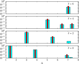
Refer to caption
(a)
Refer to caption
(b)
Figure 10: The analogue of Figure 9 for the 3D Ising model. In the fit, we have used the 2subscript2\mathbb{Z}_{2}-even operator dimensions from [47]. This is already a longer list than anything that is likely to come from a one-correlator bootstrap. Due to a remaining bias in the spectrum, there is strong disagreement between the primal and dual methods.

Turning to three dimensions, exact Ising CFT data are not available, but the tables in [47] have negligible error for our purposes. Despite all the progress in isolating this model, it appears that several spin-\ell operators are still missing from these spectra: the ones that do not fall into [σσ]nsubscriptdelimited-[]𝜎𝜎𝑛[\sigma\sigma]_{n}, [ϵϵ]nsubscriptdelimited-[]italic-ϵitalic-ϵ𝑛[\epsilon\epsilon]_{n} and [σϵ]nsubscriptdelimited-[]𝜎italic-ϵ𝑛[\sigma\epsilon]_{n} twist families. As evidence of this, Figure 10 shows that OPE coefficients fit with the dual method differ greatly from the ones returned by spectrum.py. To guess where the first missing operator appears, we can take the naive view that twist families exist all the way down to =00\ell=0. Constructing one out of an irrelevant operator ΦΦ\Phi, we have Δ2ΔΦ+2n+>2dΔ2subscriptΔΦ2𝑛2𝑑\Delta\approx 2\Delta_{\Phi}+2n+\ell>2d. Four-point functions approximated by bootstrap data have already proven useful for conformal perturbation theory and measuring non-Gaussianity [82, 83]. As it is significantly affected by the incompleteness of the spectrum above Δ2dsubscriptΔ2𝑑\Delta_{*}\approx 2d, a fit to the crossing equations must be a less forgiving problem.

Although we have not done so in this work, it should also be possible to fit mixed OPE coefficients in a 2D theory. The last two rows of (B.3) would lead to coupled quadratic equations which rapidly become impractical to solve as our system grows. Therefore, we will focus on the third row. If only the identity has been singled out, this is a homogenous equation and its parameters are ambiguous up to a rescaling. This is why it helps to find OPE coefficients in a prescribed order. As long as λϕϕϕ2subscript𝜆italic-ϕitalic-ϕsuperscriptitalic-ϕ2\lambda_{\phi\phi\phi^{2}} has been found from the ϕ×ϕitalic-ϕitalic-ϕ\phi\times\phi fit described above, permutation symmetry of this coefficient may be used to make our equation inhomogeneous. In this case, it takes the form of (B.22) but now with

aksubscript𝑎𝑘\displaystyle a_{k} =\displaystyle= λϕϕ2𝒪k2subscriptsuperscript𝜆2italic-ϕsuperscriptitalic-ϕ2subscript𝒪𝑘\displaystyle\lambda^{2}_{\phi\phi^{2}\mathcal{O}_{k}}
FksubscriptF𝑘\displaystyle\textbf{F}_{k} =\displaystyle= F,Δk,kϕϕ2;ϕϕ2subscriptsuperscriptFitalic-ϕsuperscriptitalic-ϕ2italic-ϕsuperscriptitalic-ϕ2subscriptΔ𝑘subscript𝑘\displaystyle\textbf{F}^{\phi\phi^{2};\phi\phi^{2}}_{-,\Delta_{k},\ell_{k}}
n =\displaystyle= λϕϕ2ϕ2F,Δϕ,0ϕϕ2;ϕϕ2.subscriptsuperscript𝜆2italic-ϕsuperscriptitalic-ϕ2italic-ϕsubscriptsuperscriptFitalic-ϕsuperscriptitalic-ϕ2italic-ϕsuperscriptitalic-ϕ2subscriptΔitalic-ϕ0\displaystyle-\lambda^{2}_{\phi\phi^{2}\phi}\textbf{F}^{\phi\phi^{2};\phi\phi^{2}}_{-,\Delta_{\phi},0}\;. (B.32)

Essentially, ϕitalic-ϕ\phi plays the same role that the identity operator played before.

References

  • [1] A. A. Belavin; A. M. Polyakov; A. B. Zamolodchikov. Infinite conformal symmetry in two-dimensional quantum field theory. Nuclear Physics B, 241:333–380, 1984.
  • [2] D. Friedan; Z. Qiu; S. Shenker. Conformal invariance, unitarity, and critical exponents in two dimensions. Physical Review Letters, 52(18):1575–1578, 1984.
  • [3] D. Friedan; Z. Qiu; S. Shenker. Details of the non-unitarity proof for highest weight representations of the Virasoro algebra. Communications in Mathematical Physics, 107:535–542, 1986.
  • [4] P. Goddard; A. Kent; D. Olive. Virasoro algebras and coset space models. Physics Letters B, 152(88), 1985.
  • [5] P. Goddard; A. Kent; D. Olive. Unitary representations of the Virasor and super-Virasoro algebras. Communications in Mathematical Physics, 103:105–119, 1986.
  • [6] R. Rattazzi; S. Rychkov; E. Tonni; A. Vichi. Bounding scalar operator dimensions in 4D CFT. Journal of High Energy Physics, 12(31), 2008. arXiv:0807.0004.
  • [7] S. Rychkov; A. Vichi. Universal constraints on conformal operator dimensions. Physical Review D, 80(4), 2009. arXiv:0905.2211.
  • [8] F. Caracciolo; S. Rychkov. Rigorous limits on the interaction strength in quantum field theory. Physical Review D, 81(8), 2010. arXiv:0912.2726.
  • [9] R. Rattazzil S. Rychkov; A. Vichi. Central charge bounds in 4D conformal field theory. Physical Review D, 83(4), 2011. arXiv:1009.2725.
  • [10] R. Rattazzil S. Rychkov; A. Vichi. Bounds in 4D conformal field theories with global symmetry. Journal of Physics A, 44(3), 2011. arXiv:1009.5985.
  • [11] A. Vichi. Improved bounds for CFTs with global symmetries. Journal of High Energy Physics, 1(162), 2012. arXiv:1106.4037.
  • [12] D. Poland; D. Simmons-Duffin. Bounds on 4D conformal and superconformal field theories. Journal of High Energy Physics, 5(17), 2010. arXiv:1009.2087.
  • [13] D. Poland; D. Simmons-Duffin; A. Vichi. Carving out the space of 4D CFTs. Journal of High Energy Physics, 5(110), 2012. arXiv:1109.5176.
  • [14] F. Kos; D. Poland; D. Simmons-Duffin. Bootstrapping mixed correlators in the 3D Ising model. Journal of High Energy Phyiscs, 11(109), 2014. arXiv:1406.4858.
  • [15] D. Simmons-Duffin. A semidefinite program solver for the conformal bootstrap. Journal of High Energy Physics, 6(174), 2015. arXiv:1502.02033.
  • [16] F. Kos; D. Poland; D. Simmons-Duffin; A. Vichi. Precision islands in the Ising and O(N) models. Journal of High Energy Physics, 8(36), 2016. arXiv:1603.04436.
  • [17] P. Liendo; L. Rastelli; B. C. van Rees. The bootstrap program for boundary CFTd. Journal of High Energy Physics, 7(113), 2013. arXiv:1210.4258.
  • [18] Al. B. Zamolodchikov. Three-point function in the minimal Liouville gravity. Theoretical and Mathematical Physics, 142(2):183–196, 2005.
  • [19] A. A. Belavin; A. B. Zamolodchikov. Moduli integrals and ground ring in minimal Liouville gravity. Journal of Experimental and Theoretical Physics Letters, 82(1):7–13, 2005.
  • [20] S. Ribault. Conformal field theory on the plane. 2014. arXiv:1406.4290.
  • [21] M. Hogervorst; B. C. van Rees. Crossing symmetry in alpha space. Journal of High Energy Physics, 11(193), 2017. arXiv:1702.08471.
  • [22] M. Hogervorst. Crossing kernels for boundary and crosscap CFTs. 2017. arXiv:1703.08159.
  • [23] I. Esterlis; A. L. Fitzpatrick; D. Ramirez. Closure of the operator product expansion in the non-unitary bootstrap. Journal of High Energy Physics, 11(30), 2016. arXiv:1606.07458.
  • [24] F. Gliozzi. More constraining conformal bootstrap. Physical Review Letters, 111:161602, 2013. arXiv:1307.3111.
  • [25] F. Gliozzi; A. Rago. Critical exponents of the 3d Ising and related models from the conformal bootstrap. Journal of High Energy Physics, 10(42), 2014. arXiv:1403.6003.
  • [26] F. Gliozzi; P. Liendo; M. Meineri; A. Rago. Boundary and interface CFTs from the conformal bootstrap. Journal of High Energy Physics, 5(36), 2015. arXiv:1502.07217.
  • [27] D. Simmons-Duffin. TASI lectures on the conformal bootstrap. 2016. arXiv:1602.07982.
  • [28] A. Vichi. A new method to explore conformal field theories in any dimension. PhD thesis, École Polytechnique Fédérale de Lausanne, 2011.
  • [29] S. El-Showk; M. F. Paulos. Bootstrapping conformal field theories with the extremal functional method. Physical Review Letters, 111:241601, 2013. arXiv:1211.2810.
  • [30] R. Koekoek; R. F. Swarttouw. The Askey-scheme of hypergeometric orthogonal polynomials and its q-analogue. Reports of the Faculty of Technical Mathematics and Informatics, 94(5), 1996. math/9602214.
  • [31] R. Gopakumar; A. Kaviraj; K. Sen; A. Sinha. A Mellin space approach to the conformal bootstrap. Journal of High Energy Physics, 5(27), 2017. arXiv:1611.08407.
  • [32] W. Chu. Analytical formulae for extended F23subscriptsubscript𝐹23{}_{3}{F}_{2}-series of Watson-Whipple-Dixon with two extra integer parameters. Mathematics of Computation, 81(277):467–479, 2012.
  • [33] D. Mazáč. Analytic bounds and emergence of AdS2 physics from the conformal bootstrap. Journal of High Energy Physics, 4(146), 2017. arXiv:1611.10060.
  • [34] S. Caron-Huot. Analyticity in spin in conformal theories. Journal of High Energy Physics, 9(78), 2017. arXiv:1703.00278.
  • [35] P. Desrosiers; L. Lapointe; P. Mathieu. Superconformal field theory and Jack superpolynomials. Journal of High Energy Physics, 9(37), 2012. arXiv:1205.0784.
  • [36] A. A. Belavin; M. A. Bershtein; G. M. Tarnopolsky. Bases in coset conformal field theory from AGT correspondence and Macdonald polynomials at the roots of unity. Journal of High Energy Physics, 3(19), 2013. arXiv:1211.2788.
  • [37] L. Alarie-Vezina; P. Desrosiers; P. Mathieu. Ramond singular vectors and Jack superpolynomials. Journal of Physics A, 47(3), 2013. arXiv:1309.7965.
  • [38] V. S. Dotsenko; V. A. Fateev. Conformal algebra and multipoint correlation functions in 2D statistical models. Nulear Physics B, 240:312–348, 1984.
  • [39] V. S. Dotsenko; V. A. Fateev. Four point correlation functions and the operator algebra in the two-dimensional conformal invariant theories with central charge c1𝑐1c\leq 1. Nulear Physics B, 251:691–734, 1985.
  • [40] V. S. Dotsenko; V. A. Fateev. Operator algebra of two-dimensional conformal theories with central charge c1𝑐1c\leq 1. Physics Letters B, 154:291–295, 1985.
  • [41] J. A. Wilson. Three term contiguous relations and some new orthogonal polynomials. In E. Saff; R. Varga, editor, Pade and Rational Approximations, pages 227–232. Academic Press, 1977.
  • [42] P. Suchanek. Recursive methods of determination of 4-point blocks in N=1𝑁1N=1 superconformal field theories. PhD thesis, Jagiellonian University, 2009.
  • [43] P. Furlan; A. C. Ganchev; V. B. Petkova. Fusion matrices and c<1𝑐1c<1 (quasi) local conformal theories. International Journal of Modern Physics, A5(14):2721–2735, 1990.
  • [44] M. Pawelkiewicz; V. Schomerus; P. Suchanek. The universal Racah-Wigner symbol for Uq(OSp(1|2))subscript𝑈𝑞𝑂𝑆𝑝conditional12{U_{q}}({OSp}(1|2)). Journal of High Energy Physics, 4(79), 2014. arXiv:1307.6866.
  • [45] S. El-Showk; M. F. Paulos; D. Poland; S. Rychkov; D. Simmons-Duffin; A. Vichi. Solving the 3D Ising model with the conformal bootstrap II: c-minimization and precise critical exponents. Journal of Statistical Physics, 157:869–914, 2014. arXiv:1403.4545.
  • [46] S. El-Showk; M. F. Paulos. Extremal bootstrapping: go with the flow. 2016. arXiv:1605.08087.
  • [47] D. Simmons-Duffin. The lightcone bootstrap and the spectrum of the 3d Ising CFT. Journal of High Energy Physics, 3(86), 2017. arXiv:1612.08471.
  • [48] C.-M. Chang; Y.-H. Lin. Carving out the end of the world or (superconformal bootstrap in six dimensions). Journal of High Energy Physics, 8(128), 2017. arXiv:1705.05392.
  • [49] C.-M. Chang; M. Fluder; Y.-H. Lin; Y. Wang. Spheres, charges, instantons and bootstrap: A five-dimensional odyssey. 2017. arXiv:1710.08418.
  • [50] M. Cornagliotto; M. Lemos; P. Liendo. Bootstrapping the (A1,A2)subscript𝐴1subscript𝐴2({A}_{1},{A}_{2}) Argyres-Douglas theory. Journal of High Energy Physics, 3(33), 2018. arXiv:1711.00016.
  • [51] S. Collier; P. Kravchuk; Y.-H. Lin; X. Yin. Bootstrapping the spectral function: On the uniqueness of Liouville theory and the universality of BPZ. 2017. arXiv:1702.00423.
  • [52] Y.-H. Lin; S.-H. Shao; D. Simmons-Duffin; Y. Wang; X. Yin. N=4 superconformal bootstrap of the K3 CFT. Journal of High Energy Physics, 5(126), 2017. arXiv:1511.04065.
  • [53] Y.-H. Lin; S.-H Shao; Y. Wang; X. Yin. (2,2)22(2,2) superconformal bootstrap in two dimensions. Journal of High Energy Physics, 5(112), 2017. arXiv:1610.05371.
  • [54] M. Cornagliotto; M. Lemos; V. Schomerus. Long multiplet bootstrap. Journal of High Energy Physics, 10(119), 2017. arXiv:1702.05101.
  • [55] M. F. Paulos; S. Rychkov; B. C. van Rees; B. Zan. Conformal invariance in the long-range Ising model. Nuclear Physics B, 902:296–291, 2016. arXiv:1509.00008.
  • [56] C. Behan; L. Rastelli; S. Rychkov; B. Zan. A scaling theory for the long-range to short-range crossover and an infrared duality. Journal of Physics A, 50(35), 2017. arXiv:1703.05325.
  • [57] C. Behan; L. Rastelli; S. Rychkov; B. Zan. Long-range critical exponents near the short-range crossover. Physical Review Letters, 118:241601, 2017. arXiv:1703.03430.
  • [58] M. Hogervorst; S. Rychkov; B. C. van Rees. Unitarity violation at the Wilson-Fisher fixed point in 4-epsilon dimensions. Physical Review D, 93(12), 2016. arXiv:1512.00013.
  • [59] E. Dyer; A. L. Fitzpatrick; Y. Xin. Constraints on flavored 2d CFT partition functions. Journal of High Energy Physics, 2(148), 2018. arXiv:1709.01533.
  • [60] S. Rychkov. Conformal bootstrap in three dimensions? 2011. arXiv:1111.2115.
  • [61] Z. Li; N. Su. 3D CFT archipelago from single correlator bootstrap. 2017. arXiv:1706.06960.
  • [62] V. Bashmakov; M. Bertolini; H. Raj. On non-supersymmetric conformal manifolds: field theory and holography. Journal of High Energy Physics, 11(167), 2017. arXiv:1709.01749.
  • [63] M. Baggio; N. Bobev; S. M. Chester; E. Lauria; S. S. Pufu. Decoding a three-dimensional conformal manifold. Journal of High Energy Physics, 2(62), 2018. arXiv:1712.02698.
  • [64] C. Behan. Conformal manifolds: ODEs from OPEs. 2017. arXiv:1709.03967.
  • [65] S. Hollands. Action principle for OPE. Nuclear Physics B, 926:614–638, 2018. arXiv:1710.05601.
  • [66] A. L. Fitzpatrick; J. Kaplan; D. Poland; D. Simmons-Duffin. The analytic bootstrap and AdS superhorizon locality. Journal of High Energy Physics, 12(4), 2013. arXiv:1212.3616.
  • [67] Z. Komargodski; A. Zhiboedov. Convexity and liberation at large spin. Journal of High Energy Physics, 11(140), 2013. arXiv:1212.4103.
  • [68] D. Friedan; Z. Qiu; S. Shenker. Superconformal invariance in two dimensions and the tricritical Ising model. Physics Letters B, 151:37–43, 1985.
  • [69] Z. Qiu. Supersymmetry, two-dimensional critical phenomena and the tricritical Ising model. Nuclear Physics B, 270:205–234, 1986.
  • [70] J. Rong; N. Su. Scalar CFTs and their large N limits. 2017. arXiv:1712.00985.
  • [71] A. C. Echeverri; B. von Harling; M. Serone. The effective bootstrap. Journal of High Energy Physics, 9(97), 2016. arXiv:1606.02771.
  • [72] R. Wong. Five lectures on asymptotic theory. In Z. Hua; R. Wong, editor, Differential equations and asymptotic theory in mathematical physics, pages 189–263. World Scientific, 2004.
  • [73] D. Pappadopulo; S. Rychkov; J. Espin; R. Rattazzi. OPE convergence in conformal field theory. Physical Review D, 86(10), 2012. arXiv:1208.6449.
  • [74] S. Rychkov; P. Yvernay. Remarks on the convergence properties of the conformal block expansion. Physics Letters B, 753:682–686, 2015. arXiv:1510.08486.
  • [75] E. X. W. Xia; X. M. Yao. The signs of three-term recurrence sequences. Discrete Applied Mathematics, 159:2290–2296, 2011.
  • [76] T. Hartman; S. Jain; S. Kundu. Causality constraints in conformal field theory. Journal of High Energy Physics, 5(99), 2016. arXiv:1509.00014.
  • [77] M. Hogervorst; S. Rychkov. Radial coordinates for conformal blocks. Physical Review D, 87(10), 2013. arXiv:1303.1111.
  • [78] M. Hogervorst; H. Osborn; S. Rychkov. Diagonal limit for conformal blocks in d𝑑d dimensions. Journal of High Energy Physics, 8(14), 2013. arXiv:1305.1321.
  • [79] C. Behan. PyCFTBoot: A flexible interface for the conformal bootstrap. Communications in Computational Physics, 22(1), 2017. arXiv:1602.02810.
  • [80] C. Beem; M. Lemos; P. Liendo; L. Rastelli; B. C. van Rees. The 𝒩=2𝒩2\mathcal{N}=2 superconformal bootstrap. Journal of High Energy Physics, 3(183), 2016. arXiv:1412.7541.
  • [81] W. Li. New method for conformal bootstrap with OPE truncations. 2017. arXiv:1711.09075.
  • [82] Z. Komargodski; D. Simmons-Duffin. The random-bond Ising model in 2.01 and 3 dimensions. Journal of Physics A, 50(15), 2017. arXiv:1603.04444.
  • [83] S. Rychkov; D. Simmons-Duffin; B. Zan. Non-gaussianity of the critical 3d Ising model. SciPost Physics, 2(1), 2017. arXiv:1612.02436.