Solving satisfiability using inclusion-exclusion
Abstract
Using Maple, we implement a SAT solver based on the principle of inclusion-exclusion and the Bonferroni inequalities. Using randomly generated input, we investigate the performance of our solver as a function of the number of variables and number of clauses. We also test it against Maple’s built-in tautology procedure. Finally, we implement the Lovász local lemma with Maple and discuss its applicability to SAT.
1 Introduction to SAT
First, some terminology. A Boolean variable is a variable which can take on values in , or, equivalently, (e.g. ). A literal is a Boolean variable or its negation (e.g. ). Disjunction means “or” () and conjunction means “and” (). A disjunctive clause is a disjunction of literals (e.g. ); similarly, we can define the conjunctive clause. A conjunctive normal form (CNF) is a conjunction of disjunctive clauses (e.g. ); similarly, we can define the disjunctive normal form (DNF).
We say that a CNF in the variables is satisfiable iff there exists an assignment of truth values to that makes true. For example, the CNF in the previous paragraph is satisfiable: the first clause forces ; then the second forces ; and the third forces , giving us a valid assignment. On the other hand, the CNF is, of course, not satisfiable.
Given a CNF in variables, one obvious way to determine its satisfiability is to check all assignments to the variables. There is an ongoing effort to develop more efficient algorithms to determine satisfiability. We call these algorithms “SAT solvers.” Currently, even the most efficient SAT solvers are exponential time; one can always construct worst-case scenarios that take long for the algorithm to analyze. In fact, SAT has been shown to be NP-complete, so a polynomial time SAT solver would indeed be breaking news.
Here, we shall certainly not present a polynomial-time algorithm, or even one that is practically more competent than current solvers. Rather, we wish to outline a simple, novel approach to solving SAT, analyze its strengths and weaknesses, and discuss how it might be used as the basis for a more powerful solver.
2 SAT and inclusion-exclusion
Suppose is a CNF with clauses and variables . Then, is satisfiable iff is not a tautology. So SAT can be rephrased as “given an arbitrary DNF, determine if it is a tautology.” We shall use this formulation in our approach.
Thus, let be a DNF with clauses and variables . We wish to determine if all possible assignments to the variables result in being true. We can interpret this probabilistically: If we pick a uniform random assignment, is ? Equivalently, letting be the event that is satisfied, is ?
Recall that we can compute the probability of such a union using the following:
Proposition 2.1 (Principle of Inclusion-Exclusion).
Let be events in a finite probability space. For , define
Then,
So our problem amounts to finding for arbitrary , which is easy: Let be the set of literals appearing in the clauses ; then, if contains a variable and its negation, and otherwise.
This idea is easily implemented to produce a simple SAT solver which always terminates with a correct answer. Such a solver, along with some test results, is briefly outlined in [GC].
However, notice that the sums in Proposition 2.1 grow with the number of clauses. Luckily, we have the Bonferroni inequalities, which tell us that we can compute the outer sum partially and still get a bound on the probability we are after:
Proposition 2.2 (Bonferroni Inequalities).
With the notation of Proposition 2.1, let . Then,
where means if is odd and if is even.
Using the Bonferroni inequalities and looping over , we can get a sequence of upper and lower bounds on . If at some point we find that or , then we can exit the loop and determine that is not a tautology or a tautology, respectively. In the worst case, we have to go up to , but (hopefully) we arrive at a decision after significantly less steps.
2.1 Details of the algorithm
The method outlined above is implemented in the Maple package sat.txt; see Section 5 for instructions to obtain the package.
We encode a DNF as a set of sets of integers: For example, {{1,-2},{3}} corresponds to . The Merge procedure is the equivalent of conjunction: Merge({-1,2},{2,3}) returns {-1,2,3}, while Merge({1,2},{-2,3}) returns false since these two clauses are “incompatible,” i.e., not simultaneously satisfiable.
The main procedure is Taut. It inputs a DNF S and threshold K. We initialize P=0 and N=nops(S), the number of clauses. For k from 1 to K, we compute the kth term in the inclusion-exclusion sum and add it to P. For the sake of efficiency, a table is used to keep track of all compatible conjunctions of k clauses in S, so that at the kth stage, the table has at most
N choose k entries. If we obtain a conclusive bound at some point in the loop, we return [ans,k], where the first entry is true or false, depending on whether we found S to be a tautology. If we complete the whole loop without coming to a conclusion, we return [P,k].
3 Testing the solver
To test our solver, we use the procedure RandNF(n,N,M), which generates a random DNF with N clauses in n variables, each containing M uniform random literals. By default, M=3, which we shall assume from now on.
The procedure MetaTaut(n,N,K,M) runs Taut on M random DNFs with n variables and N clauses and threshold K, and it records the run time and output of each trial.
The procedure MetaTaut(n,N,K,M) does the same, but instead of our solver, it uses Maple’s built-in tautology procedure.
3.1 Runtimes
As one would expect, our solver seems to perform most competently when there are lots of variables but not too many clauses.
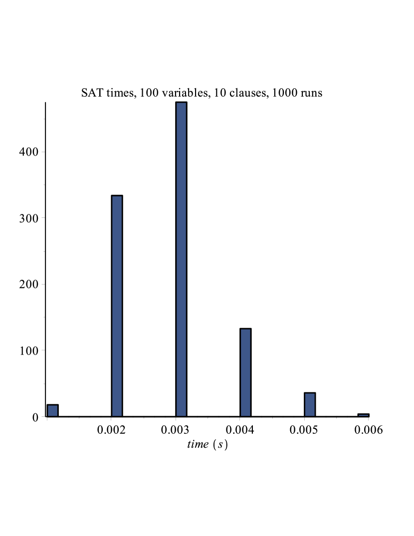
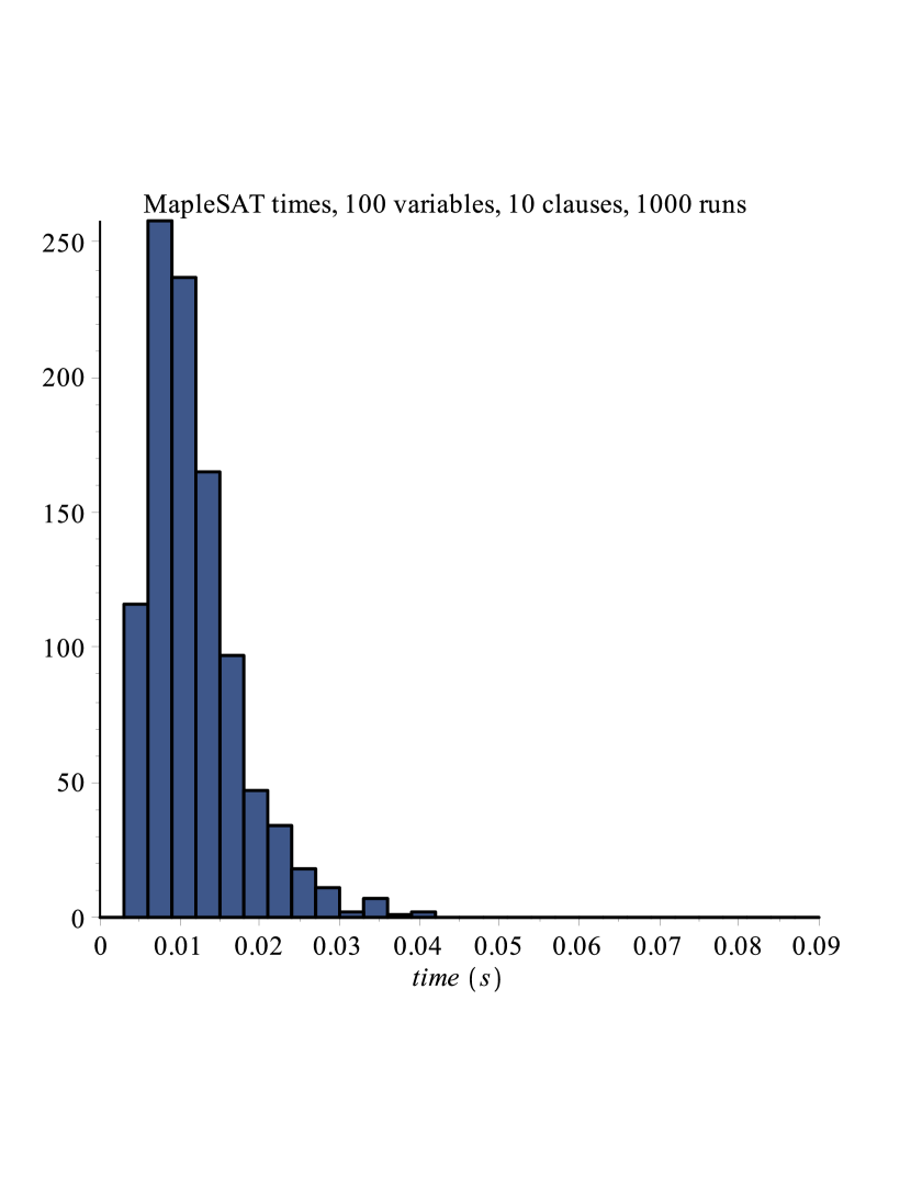
For example, Figure 1 shows a histogram of runtimes resulting from using Taut on 1000 random DNFs generated by RandNF(100,10). In all of these cases, our solver arrived at the correct answer by the third step of the loop, and the longest runtime was .006s. As Figure 1 shows, the Maple solver performed slower in this case.
Further, we tested Taut on 10 random DNFs generated by RandNF(1000,20), and it decided each of them was not a tautology by the seventh inclusion-exclusion step. The runtimes ranged from 2-58 minutes, with an average of 19. In this case, using MapleTaut resulted in an overflow error.
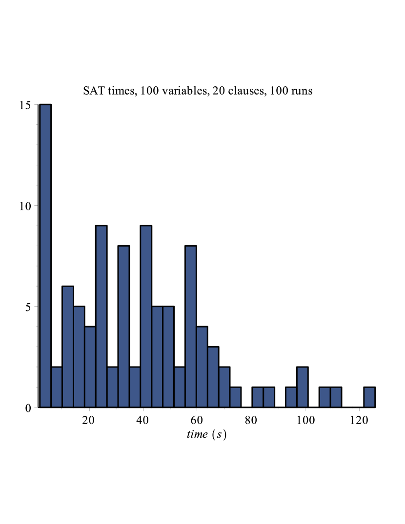
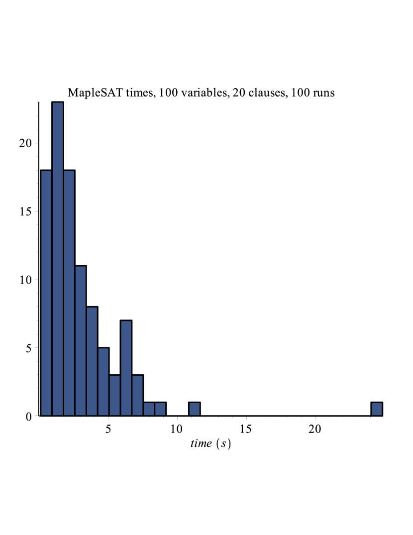
On the other hand, Figure 2 shows the results when 100 random DNFs generated by RandTaut(100,20) are used. Already, the number of clauses is enough to make our solver slower than Maple. In fact, in this case, only fifteen of the 100 random DNFs are solvable by Taut with threshold .
Also, we should point out that, in the situations where our method does seem promising, it seems that it almost always returns false. So, as it is, it probably has little practical use. Further, we are only testing it against a na ive built-in Maple tautology function, rather than a sophisticated SAT solver.
3.2 Thresholds
Recall that, in Taut(S,k), the argument k is the threshold, that is, the number of inclusion-exclusion summands computed before the procedure quits. Now, we investigate how the required threshold is related to the number of variables n and number of clauses N.
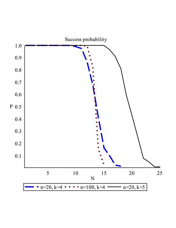
The procedure HowManyFinished(n,N,k,M) runs Taut with threshold k on M random DNFs generated by RandNF(n,N), and it outputs the proportion of conclusive runs. In other words, it estimates success probability that a DNF generated by RandNF(n,N) is solvable by our algorithm with threshold k.
Empirical evidence shows a phase shift behavior in the success probability If we fix and and vary . Namely, there appears to be a critical number of clauses at which the graph of the success probability has an inflection point. Of course, we have , with increasing in .
Some plots exhibiting this phase shift are shown in Figure 3. Note that this behavior is reminiscent of the satisfiability phase shift studied in [XW], where the behavior of the probability of a random CNF being satisfiable as a function of the ratio of the number of variables and clauses is studied.
4 SAT and the Lovász local lemma
4.1 Computerizing the local lemma
Given some “bad events” , the Lovász local lemma can be used to verify that there is a positive probability that none of them occurs. Suppose is a dependency graph on the vertex set : That is, events in are mutually independent of their non-neighbors in . Let denote the neighborhood of in . Then the following holds:
Proposition 4.1 (Asymmetric Lovász local lemma).
Suppose there exists a weight function such that
Then .
In applications, the weight function is usually found ad hoc. If we assume each vertex of the dependency graph has degree and set , we obtain the following:
Proposition 4.2 (Symmetric Lovász local lemma).
Suppose each event satisfies and is independent of all but at most of the other events. If
then .
The procedure LLLs(P,G) in the Maple package checks if the events satisfy the symmetric local lemma, where the lists and satisfy and .
Computerizing the asymmetric local lemma is harder, since, as far as we know, there is no systematic and efficient way to look for a valid weight function . Somewhat arbitrarily, the procedure LLL(P,G) uses the weight function . The motivation for this choice is that, when the dependency graph is uniform, it reduces to the symmetric local lemma.
4.2 Applying the local lemma to SAT
The article [G] addresses a theoretical application of the local lemma to SAT, focusing on using it to derive combinatorial conditions for the satisfiability of CNFs. Here, present a computer application of the local lemma to SAT.
Let us return to the setup in Section 2. We have a DNF with variables , which are assigned true/false values uniformly at random. We let be the event that is true. Then is not a tautology iff there is a positive probability that none of the events occurs. So we can apply the local lemma.
We form a dependency graph by joining and iff the clauses and have common variables. Also, , where is the number of literals in ; for example, for 3-SAT, .
The procedure DNFtoPG(S) converts the DNF to a pair , which can be passed to one of the LLL procedures. If the procedure returns true, then we can conclude that was not a tautology; otherwise, this method is inconclusive.
Unfortunately, LLLs rarely succeeds at detecting a non-tautology, and LLL is only slightly better. For example, out of 100 non-tautologies generated by RandNF(100,10), only 26 were detected by LLLs and 37 by LLL. Out of 100 non-tautologies generated by RandNF(100,15), only 2 were detected by LLLs and 3 by LLL. We expect that this is due to the behavior of the dependency graph. It would be interesting to develop a “clever” asymmetric local lemma algorithm that tailors the weight function to work for the given dependency graph.
5 Using the Maple package
The Maple package sat.txt accompanying this paper may be found at the following URL:
http://www.math.rutgers.edu/~az202/Z.
To use the Maple package, place sat.txt in the working directory and execute read(‘sat.txt‘);.
To see the main procedures, execute Help();. For help on a specific procedure, use Help(<procedure name>);.
Here are some things to try:
-
•
Taut({{-3,1,4},{-2,-1,4}},2);determines if is a tautology using inclusion-exclusion with threshold 2. -
•
MapleTaut({{-3,1,4},{-2,-1,4}});determines if is a tautology using Maple’stautologyprocedure. -
•
RandNF(10,4);generates a random DNF with approximately 10 variables and 4 clauses. -
•
MetaTaut(5,25,8,10);runsTaut(RandNF(5,25),8)10 times. -
•
LLL(DNFtoPG({{-3,1,4},{-2,-1,4}}));determines if the LLL applies to the given DNF (if true is returned, then it is not a tautology). -
•
MetaLLL(100,10,100);applies the local lemma to 100 DNFs generated byRandNF(100,10)and outputs the proportion of non-tautologies detected byLLLand the actual proportion of non-tautologies.
Acknowledgement
The author thanks Dr. Doron Zeilberger for introducing this project to him and guiding his research in the right direction.
6 References
-
[G]
Heidi Gebauer, Robin A. Moser, Dominik Scheder, and Emo Welzl, The Lovász Local Lemma and Satisfiability, in: Efficient Algorithms, Part I, pp. 30-54, Susanne Albers, Helmut Alt, and Stefan N aher (eds.). Heidelberg: Springer-Verlag, 2009.
-
[GC]
Gábor Kusper and Csaba Biró, Solving SAT by an Iterative Version of the Inclusion-Exclusion Principle, 2015 17th International Symposium on Symbolic and Numeric Algorithms for Scientific Computing (SYNASC), Timisoara, 2015, pp. 189-190.
-
[XW]
Ke Xu and Wei Li, The SAT phase transition,
http://www.math.ucsd.edu/~sbuss/CourseWeb/Math268_2007WS/satphase.pdf