Combinatorics of chemical reaction systems

Nicolas Behra, Gérard H. E. Duchampb and Karol A. Pensonc

We propose a concise stochastic mechanics framework for chemical reaction systems that allows to formulate evolution equations for three general types of data: the probability generating functions, the exponential moment generating functions and the factorial moment generating functions. This formulation constitutes an intimate synergy between techniques of statistical physics and of combinatorics. We demonstrate how to analytically solve the evolution equations for all six elementary types of single-species chemical reactions by either combinatorial normal-ordering techniques, or, for the binary reactions, by means of Sobolev-Jacobi orthogonal polynomials. The former set of results in particular highlights the relationship between infinitesimal generators of stochastic evolution and parametric transformations of probability distributions.

footnotetext: a Institut de Recherche en Informatique Fondamentale (IRIF), Université Paris-Diderot (Paris 07), France; E-Mail: nicolas.behr@irif.frfootnotetext: b Université Paris 13, Sorbonne Paris Cité, LIPN, CNRS UMR 7030, F-93430 Villetaneuse, France; E-Mail: ghed@lipn.univ-paris13.frfootnotetext: c Laboratoire de Physique Theorique de la Matière Condensée (LPTMC), CNRS UMR 7600, Sorbonne Universités, Université Pierre et Marie Curie (Paris 06), France; E-Mail: penson@lptl.jussieu.fr

1 Introduction

Intended as an invitation to interdisciplinary researchers and in particular to combinatorists, we present in this work an extension of the early work of Delbrück [1] on probability generating functions for chemical reaction systems to a so-called stochastic mechanics framework. While the idea to study chemical reaction systems in terms of probability generating functions is thus not new, and on the contrary constitutes one of the standard techniques of this field (see e.g. [2] for a historical compendium), we believe that the reformulation of these techniques in terms of the stochastic mechanics formalism could lead to fruitful interaction of a broader audience. In the spirit of the ideas presented by M. Doi in his seminal paper [3], the main motivation for such a reformulation lies in a clear conceptual separation of (i) the state space of the system and (ii) the linear operators implementing the evolution of the system. Combined with insights obtained in a recent study of stochastic graph rewriting systems [4, 5, 6], one may add to this list (iii) the linear operators that implement observable quantities. It is only through combining this Ansatz with the standard notions of combinatorial generating functions that we find the true strengths of the stochastic mechanics approach: providing an avenue to obtain exact solutions to dynamical evolution equations. Combinatorists will recognize in our formulation of evolution equations intrinsic notions of normal-ordering problems, and indeed certain semi-linear normal-ordering techniques [7, 8, 9, 10] will prove immensely fruitful in this direction. Chemists and other practitioners might appreciate that our solutions not only provide asymptotic information on the time-evolution of the reaction systems, but also provide full information on the evolution of reaction systems from any initial state at time t=0𝑡0t=0 to any desired time t=T𝑡𝑇t=T (with T>0𝑇0T>0). While many individual results on such time-evolutions are known in the literature [2, 11], we hope that our concise formalism may help to consolidate the knowledge on the mathematical methods involved in deriving such exact results, and in some cases even extend the current knowledge. Amongst the novel technical results in this paper we present an exact solution to single-species binary chemical reaction systems. This result is obtained via a necessary modification of an Ansatz by McQuarrie [12] via so-called Sobolev-Jacobi orthogonal polynomials, which have been introduced in the work of Kwon and Littlejohn [13, 14, 15, 16].

For clarity of exposition, we will first present the general theory of so-called continuous-time Markov chains (CTMCs) [17] in our framework of stochastic mechanics. This approach to the theory of CTMCs has the advantage of giving clear intuitions as familiar from the general theory of statistical physics to the types of computations that arise. It moreover admits an entry point to non-specialists that we think is somewhat more accessible than the vast standard literature on the topic. We will then present a derivation of a framework to describe chemical reaction systems, and illustrate how to obtain exact closed-form solutions to the evolution equations of certain types of reaction systems.

2 The stochastic mechanics formalism

As a preparation for the main part of this paper, we begin with a short survey of some of the standard notions of continuous time Markov chain (CTMC) theory [17] and related notions of probability theory. Due to a certain (albeit superficial) similarity of many of the formulae of interest to those of quantum mechanics, following [18] we will refer to this framework as stochastic mechanics. In particular, some of the notations we will use are inspired by those common in quantum mechanics.

We will be concerned with the study of systems whose space of pure states (i.e. of concrete configurations) is described in the following manner:

Definition 1.

For a stochastic dynamical system, let S𝑆S denote the vector space (over \mathbb{R}) spanned by the pure states (basis vectors) |sSket𝑠𝑆\left|s\right\rangle\in S. Typically, S𝑆S is countably infinite dimensional. A mixed state |ΨProb(S)ketΨ𝑃𝑟𝑜𝑏𝑆\left|\Psi\right\rangle\in Prob(S) of the system is a probability distribution over S𝑆S, with Prob(S)𝑃𝑟𝑜𝑏𝑆Prob(S) defined as

Prob(S)𝑃𝑟𝑜𝑏𝑆\displaystyle Prob(S) :={|Ψ=sψs|s,\displaystyle:=\bigg{\{}\left|\Psi\right\rangle=\sum_{s}\psi_{s}\left|s\right\rangle\,, (1)
ψs0andsψs=1}.\displaystyle\qquad\qquad\psi_{s}\in\mathbb{R}_{\geq 0}\;\text{and}\;\sum_{s}\psi_{s}=1\bigg{\}}\,.

Elements of Prob(S)𝑃𝑟𝑜𝑏𝑆Prob(S) may thus in particular be seen as special elements of the space 1(S)subscriptsuperscript1𝑆\ell^{1}_{\mathbb{R}}(S) (absolutely 1subscriptsuperscript1\ell^{1}_{\mathbb{R}}-summable series over S𝑆S),

1(S)subscriptsuperscript1𝑆\displaystyle\ell^{1}_{\mathbb{R}}(S) :={|Ψ=sψs|s,\displaystyle:=\bigg{\{}\left|\Psi\right\rangle=\sum_{s}\psi_{s}\left|s\right\rangle\,, (2)
ψsands|ψs|<}.\displaystyle\qquad\quad\psi_{s}\in\mathbb{R}\;\text{and}\;\sum_{s}|\psi_{s}|<\infty\bigg{\}}\,.

For later convenience, we introduce an operation |bra\left\langle\mathcal{R}\right| via its action on basis vectors,

|s:=1for all |sS,formulae-sequenceassigninner-product𝑠1for all ket𝑠𝑆\left\langle\left.\mathcal{R}\right|s\right\rangle:=1\quad\text{for all }\left|s\right\rangle\in S\,, (3)

which extends by linearity to

|Ψ=sψs|s=sψs.inner-productΨsubscript𝑠subscript𝜓𝑠inner-product𝑠subscript𝑠subscript𝜓𝑠\left\langle\left.\mathcal{R}\right|\Psi\right\rangle=\sum_{s}\psi_{s}\left\langle\left.\mathcal{R}\right|s\right\rangle=\sum_{s}\psi_{s}\,. (4)

In other words, |bra\left\langle\mathcal{R}\right| implements the summation of coefficients when applied to a distribution |ΨketΨ\left|\Psi\right\rangle over S𝑆S.

The reader is cautioned not to take the analogy to the notations of quantum mechanics too far in interpreting the notation |sinner-product𝑠\left\langle\left.\mathcal{R}\right|s\right\rangle as a form of scalar product. In fact, since this is a rather crucial point, we provide in Appendix A a direct comparison of the notions of stochastic mechanics as opposed to the notions of quantum mechanics. For the purposes of stochastic mechanics, we thus merely treat |bra\left\langle\mathcal{R}\right| as a convenient (and standard***Some alternative notations frequently encountered in the literature [3, 19, 20] include ||P||.\left\langle\mathcal{R}\right|\equiv\left\langle\right|\equiv\left\langle P\right|\equiv\left\langle-\right|\,. ) shorthand notation.

We now turn to one of the core concepts of the stochastic mechanics framework:

Definition 2 (cf. e.g. [17]).

Let S𝑆S denote a vector space of pure states, and let Prob(S)𝑃𝑟𝑜𝑏𝑆Prob(S) denote the space of probability distributions over S𝑆S (cf. Definition 1). Then a continuous time Markov chain (CTMC) over S𝑆S is defined in terms of providing an input state

|Ψ(0)Prob(S)ketΨ0𝑃𝑟𝑜𝑏𝑆\left|\Psi(0)\right\rangle\in Prob(S) (5)

and a one-parameter evolution semi-group (t)𝑡\mathcal{E}(t), where t[0,)𝑡0t\in[0,\infty). (t)𝑡\mathcal{E}(t) possesses the following defining properties (for all non-negative real parameters s,t0𝑠𝑡subscriptabsent0s,t\in\mathbb{R}_{\geq 0}):

(0)0\displaystyle\mathcal{E}(0) =𝟙absentdouble-struck-𝟙\displaystyle=\mathbb{1} (6a)
(s+t)𝑠𝑡\displaystyle\mathcal{E}(s+t) =(s)(t)=(t)(s)absent𝑠𝑡𝑡𝑠\displaystyle=\mathcal{E}(s)\mathcal{E}(t)=\mathcal{E}(t)\mathcal{E}(s) (6b)
ddt(t)𝑑𝑑𝑡𝑡\displaystyle\frac{d}{dt}\mathcal{E}(t) =H(t)=(t)H.absent𝐻𝑡𝑡𝐻\displaystyle=H\mathcal{E}(t)=\mathcal{E}(t)H\,. (6c)

Here, the first two equations express the semi-group property of \mathcal{E}, while (6c) expresses the Markov property (i.e. memorylessness) itself, with H𝐻H the infinitesimal generator of \mathcal{E}. Then the time-dependent state |Ψ(t)Prob(S)ketΨ𝑡𝑃𝑟𝑜𝑏𝑆\left|\Psi(t)\right\rangle\in Prob(S) of the CTMC𝐶𝑇𝑀𝐶CTMC is given by

|Ψ(t)=(t)|Ψ(0).ketΨ𝑡𝑡ketΨ0\left|\Psi(t)\right\rangle=\mathcal{E}(t)\left|\Psi(0)\right\rangle\,. (7)

Owing to (6c), |Ψ(t)ketΨ𝑡\left|\Psi(t)\right\rangle satisfies the so-called Master equation or Kolmogorov backwards equation,

ddt|Ψ(t)=H|Ψ(t).𝑑𝑑𝑡ketΨ𝑡𝐻ketΨ𝑡\frac{d}{dt}\left|\Psi(t)\right\rangle=H\left|\Psi(t)\right\rangle\,. (8)

Since the infinitesimal generator H𝐻H thus bears a certain formal resemblance in its role to the Hamiltonian in the quantum mechanics setting, we will (by an abuse of terminology as illustrated in Appendix A) refer to it as Hamiltonian also in the stochastic mechanics setting.

The definition of a continuous-time Markov chain thus comprises the information on what are the pure states of the stochastic dynamical system, and on what are the possible transitions of the system. The transitions in turn would typically implement the notions of, say, chemical reactions or other changes of configurations of states. In practice, the precise nature of these transitions will determine the structure of the infinitesimal generator H𝐻H. We will provide an in-detail discussion of the infinitesimal generators in the case of chemical reaction systems in the main part of this paper.

It might be worth pointing out that the systems thus defined are in a certain sense dimensionless, i.e. there is no notion of physical space implied by the definitions. However, as for example realized in the famous Doi-Peliti formalism [3, 20], it is possible to extend the concept of pure states to include a notion of space e.g. in the form of configurations over a lattice of positions in physical space, and even to consider taking a certain limit of zero lattice spacing to recover a notion of continuous space.

As we will see in the sequel, the Hamiltonian H𝐻H of a CTMC can in general turn out to be an unbounded operator acting on a countably infinite-dimensional space, whence considerable care is necessary in order to understand the precise mathematical meaning of the CTMC definitions and of the evolution semigroup. While in the case of a finite state-space we simply find the relation (see e.g. [21] and references therein)

(t)=etH,𝑡superscript𝑒𝑡𝐻\mathcal{E}(t)=e^{tH}\,, (9)

for unbounded operators H𝐻H such an expression would quite possibly not be mathematically well-posed. In the general cases, one therefore needs to resort to more intricate concepts such as the Hille-Yosida theory of functional analysis. We refer the interested readers to the standard literature on the subject (see e.g. [22, 23, 24]) for the full mathematical details. Here, we content ourselves with stating a number of abstract properties of the infinitesimal generators H𝐻H that will prove useful to our framework in the following.

Lemma 1.

Given a CTMC over some state space S𝑆S with initial state |Ψ(0)Prob(S)ketΨ0𝑃𝑟𝑜𝑏𝑆\left|\Psi(0)\right\rangle\in Prob(S), evolution semi-group \mathcal{E} and infinitesimal generator H𝐻H, we have that

|H=0.bra𝐻0\left\langle\mathcal{R}\right|H=0\,. (10)
Proof.

Recall that since for all t0𝑡0t\geq 0 the state |Ψ(t)ketΨ𝑡\left|\Psi(t)\right\rangle of the CTMC is a probability distribution, it satisfies

|Ψ(t)=sψs=1.inner-productΨ𝑡subscript𝑠subscript𝜓𝑠1\left\langle\left.\mathcal{R}\right|\Psi(t)\right\rangle=\sum_{s}\psi_{s}=1\,.

This entails in particular that

0=ddt|Ψ(t)0𝑑𝑑𝑡inner-productΨ𝑡\displaystyle 0=\frac{d}{dt}\left\langle\left.\mathcal{R}\right|\Psi(t)\right\rangle =ddt|(t)|Ψ(0)absent𝑑𝑑𝑡quantum-operator-product𝑡Ψ0\displaystyle=\frac{d}{dt}\left\langle\mathcal{R}\right|\mathcal{E}(t)\left|\Psi(0)\right\rangle
=(6c)|H(t)|Ψ(0).italic-(6citalic-)quantum-operator-product𝐻𝑡Ψ0\displaystyle\overset{\eqref{eq:CTMCdiff}}{=}\left\langle\mathcal{R}\right|H\mathcal{E}(t)\left|\Psi(0)\right\rangle\,.

But since this must hold for arbitrary times t0𝑡0t\geq 0, the claim (10) follows. ∎

2.1 Advantages of the stochastic mechanics formulation

We will now present some of the key strengths of the formulation of CTMCs in terms of the stochastic mechanics formalism, a point which we will elaborate further when entering the discussion of chemical reaction systems.

One of the main advantages of the formalism is the ability to compute naturally (and in many cases even in closed form) quantities of interest in practical applications, namely the moments of observables. Since part of the computations for chemical reactions will involve additional mathematical structures, we choose to first present some of the general concepts here.

Suppose then that we are studying a continuous-time Markov chain (CTMC) with space of pure states S𝑆S, initial state |Ψ(0)Prob(S)ketΨ0𝑃𝑟𝑜𝑏𝑆\left|\Psi(0)\right\rangle\in Prob(S), evolution semi-group (t)𝑡\mathcal{E}(t) and infinitesimal generator H𝐻H as before.

Definition 3.

An observable O𝑂O for a CTMC is a diagonal linear operator on S𝑆S, whence for all pure states |sSket𝑠𝑆\left|s\right\rangle\in S

O|s=ωs(O)|s(ωs(O)).𝑂ket𝑠subscript𝜔𝑠𝑂ket𝑠subscript𝜔𝑠𝑂O\left|s\right\rangle=\omega_{s}(O)\left|s\right\rangle\quad(\omega_{s}(O)\in\mathbb{R})\,. (11)

We denote the space of observables on S𝑆S by 𝒪(S)𝒪𝑆\mathcal{O}(S).

Since the observables are thus by definition diagonal in the basis of pure states, any two observables O1,O2𝒪(S)subscript𝑂1subscript𝑂2𝒪𝑆O_{1},O_{2}\in\mathcal{O}(S) commute:

[O1,O2]=O1O2O2O1=0.subscript𝑂1subscript𝑂2subscript𝑂1subscript𝑂2subscript𝑂2subscript𝑂10[O_{1},O_{2}]=O_{1}O_{2}-O_{2}O_{1}=0\,. (12)

Consider now a fixed (finite) set of observables {O1,,On}subscript𝑂1subscript𝑂𝑛\{O_{1},\dotsc,O_{n}\}, with Oi𝒪(S)subscript𝑂𝑖𝒪𝑆O_{i}\in\mathcal{O}(S). Let us introduce the convenient multi-index notation

x¯:=(x1,,xn)assign¯𝑥subscript𝑥1subscript𝑥𝑛\underline{x}:=(x_{1},\dotsc,x_{n})

for vectors and

λ¯O¯:=i=1nλiOiassign¯𝜆¯𝑂superscriptsubscript𝑖1𝑛subscript𝜆𝑖subscript𝑂𝑖\underline{\lambda}\cdot\underline{O}:=\sum_{i=1}^{n}\lambda_{i}O_{i} (13)

for linear combinations of observables. Here, we will either consider real coefficients λisubscript𝜆𝑖\lambda_{i}\in\mathbb{R} or formal coefficients (such as e.g. in Definition 5). We will also make use of the shorthand notation

O¯m¯:=i=1nOimi,assignsuperscript¯𝑂¯𝑚superscriptsubscriptproduct𝑖1𝑛superscriptsubscript𝑂𝑖subscript𝑚𝑖\underline{O}^{\underline{m}}:=\prod_{i=1}^{n}O_{i}^{m_{i}}\,, (14)

with (finite) non-negative integer exponents misubscript𝑚𝑖m_{i}.

Denoting by |Ψ(t)=(t)|Ψ(0)ketΨ𝑡𝑡ketΨ0\left|\Psi(t)\right\rangle=\mathcal{E}(t)\left|\Psi(0)\right\rangle the time-dependent state of the system, we may now define in complete analogy to standard probability theory the concept of expectation values of observables, commonly referred to as moments:

Definition 4.

For a given choice of exponents m1,,mnsubscript𝑚1subscript𝑚𝑛m_{1},\dotsc,m_{n}, we define

O¯m¯(t):=|O1m1Onmn|Ψ(t).assigndelimited-⟨⟩superscript¯𝑂¯𝑚𝑡quantum-operator-productsuperscriptsubscript𝑂1subscript𝑚1superscriptsubscript𝑂𝑛subscript𝑚𝑛Ψ𝑡\left\langle\underline{O}^{\underline{m}}\right\rangle(t):=\left\langle\mathcal{R}\right|O_{1}^{m_{1}}\cdots\dotsc\cdots O_{n}^{m_{n}}\left|\Psi(t)\right\rangle\,. (15)

For example, the expectation value of a single observable Oisubscript𝑂𝑖O_{i} in state |Ψ(t)ketΨ𝑡\left|\Psi(t)\right\rangle, in the traditional probability theory literature sometimes denoted 𝔼|Ψ(t)(Oi)subscript𝔼ketΨ𝑡subscript𝑂𝑖\mathbb{E}_{\left|\Psi(t)\right\rangle}(O_{i}), would thus read

𝔼|Ψ(t)(Oi)subscript𝔼ketΨ𝑡subscript𝑂𝑖\displaystyle\mathbb{E}_{\left|\Psi(t)\right\rangle}(O_{i}) Oi(t)=|𝒪i|Ψ(t)absentdelimited-⟨⟩subscript𝑂𝑖𝑡quantum-operator-productsubscript𝒪𝑖Ψ𝑡\displaystyle\equiv\langle O_{i}\rangle(t)=\left\langle\mathcal{R}\right|\mathcal{O}_{i}\left|\Psi(t)\right\rangle
=sψs(t)|Oi|sabsentsubscript𝑠subscript𝜓𝑠𝑡quantum-operator-productsubscript𝑂𝑖𝑠\displaystyle=\sum_{s}\psi_{s}(t)\left\langle\mathcal{R}\right|O_{i}\left|s\right\rangle
=(11)sψs(t)ωs(Oi)|sitalic-(11italic-)subscript𝑠subscript𝜓𝑠𝑡subscript𝜔𝑠subscript𝑂𝑖inner-product𝑠\displaystyle\overset{\eqref{eq:ObsDef}}{=}\sum_{s}\psi_{s}(t)\omega_{s}(O_{i})\left\langle\left.\mathcal{R}\right|s\right\rangle
=sψs(t)ωs(Oi).absentsubscript𝑠subscript𝜓𝑠𝑡subscript𝜔𝑠subscript𝑂𝑖\displaystyle=\sum_{s}\psi_{s}(t)\omega_{s}(O_{i})\,.
Definition 5.

With notations as above, the exponential generating function (EGF) (t;λ¯)𝑡¯𝜆\mathcal{M}(t;\underline{\lambda}) for the moments of the set of observables {O1,,Om}subscript𝑂1subscript𝑂𝑚\{O_{1},\dotsc,O_{m}\} of the system with time-dependent state |Ψ(t)ketΨ𝑡\left|\Psi(t)\right\rangle is defined as

(t;λ¯)𝑡¯𝜆\displaystyle\mathcal{M}(t;\underline{\lambda}) :=eλ¯O¯(t)assignabsentdelimited-⟨⟩superscript𝑒¯𝜆¯𝑂𝑡\displaystyle:=\left\langle e^{\underline{\lambda}\cdot\underline{O}}\right\rangle(t) (16)
=m01m!|(λ¯O¯)m|Ψ(t).absentsubscript𝑚01𝑚quantum-operator-productsuperscript¯𝜆¯𝑂𝑚Ψ𝑡\displaystyle=\sum_{m\geq 0}\frac{1}{m!}\left\langle\mathcal{R}\right|(\underline{\lambda}\cdot\underline{O})^{m}\left|\Psi(t)\right\rangle\,.

Arbitrary moments may be computed from (t;λ¯)𝑡¯𝜆\mathcal{M}(t;\underline{\lambda}) according to

O1m1Onmn(t)delimited-⟨⟩superscriptsubscript𝑂1subscript𝑚1superscriptsubscript𝑂𝑛subscript𝑚𝑛𝑡\displaystyle\left\langle O_{1}^{m_{1}}\cdots\dotsc\cdots O_{n}^{m_{n}}\right\rangle(t) (17)
=[m1λ1m1mnλ1mn(t;λ¯)]|λ¯0¯.absentevaluated-atdelimited-[]superscriptsubscript𝑚1superscriptsubscript𝜆1subscript𝑚1superscriptsubscript𝑚𝑛superscriptsubscript𝜆1subscript𝑚𝑛𝑡¯𝜆¯𝜆¯0\displaystyle\qquad=\left[\frac{\partial^{m_{1}}}{\partial\lambda_{1}^{m_{1}}}\dotsc\frac{\partial^{m_{n}}}{\partial\lambda_{1}^{m_{n}}}\mathcal{M}(t;\underline{\lambda})\right]\bigg{|}_{\underline{\lambda}\to\underline{0}}\,.

In other words, knowing the exponential moment-generating function (t;λ¯)𝑡¯𝜆\mathcal{M}(t;\underline{\lambda}) for the observables of interest in a given system amounts typically to knowing all relevant stochastic dynamical properties of the system.

Finally, we are now in a position to assemble all concepts introduced thus far into one of the cornerstones of this paper (see [4] for the original version of this result, formulated in the framework of rule algebras invented by the first named author, and [6] for its most general variant):

Theorem 1.

For a CTMC with space of pure states S𝑆S, initial state |Ψ(0)Prob(S)ketΨ0𝑃𝑟𝑜𝑏𝑆\left|\Psi(0)\right\rangle\in Prob(S), evolution semi-group (t)𝑡\mathcal{E}(t) and infinitesimal generator H𝐻H, the exponential moment-generating function (t;λ¯)𝑡¯𝜆\mathcal{M}(t;\underline{\lambda}) for a given (finite) set of observables {O1,,On}subscript𝑂1subscript𝑂𝑛\{O_{1},\dotsc,O_{n}\} (with Oi𝒪(S)subscript𝑂𝑖𝒪𝑆O_{i}\in\mathcal{O}(S)) fulfills the evolution equation

t(t;λ¯)=q11q!|(ad(λ¯O¯)qH)eλ¯O¯|Ψ(t).𝑡𝑡¯𝜆subscript𝑞11𝑞quantum-operator-product𝑎superscriptsubscript𝑑¯𝜆¯𝑂absent𝑞𝐻superscript𝑒¯𝜆¯𝑂Ψ𝑡\tfrac{\partial}{\partial t}\mathcal{M}(t;\underline{\lambda})=\sum_{q\geq 1}\frac{1}{q!}\,\left\langle\mathcal{R}\right|\left(ad_{(\underline{\lambda}\cdot\underline{O})}^{\circ\>q}\>H\right)e^{\underline{\lambda}\cdot\underline{O}}\left|\Psi(t)\right\rangle\,. (18)

Here, for two linear operators A𝐴A and B𝐵B the notation adAB𝑎subscript𝑑𝐴𝐵ad_{A}B stands for the adjoint action (commutator),

adAB:=[A,B]=ABBA,assign𝑎subscript𝑑𝐴𝐵𝐴𝐵𝐴𝐵𝐵𝐴ad_{A}B:=[A,B]=AB-BA\,,

while adAqB𝑎superscriptsubscript𝑑𝐴absent𝑞𝐵ad_{A}^{\circ\>q}\>B denotes the q𝑞q-fold commutator (q>1𝑞1q>1),

adAqB𝑎superscriptsubscript𝑑𝐴absent𝑞𝐵\displaystyle ad_{A}^{\circ\>q}\>B :=(adAadA)q times(B)assignabsentsubscript𝑎subscript𝑑𝐴𝑎subscript𝑑𝐴q times𝐵\displaystyle:=\underbrace{(ad_{A}\circ\dotsc\circ ad_{A})}_{\text{$q$ times}}(B)
=[A,[A,,[A,B]]]q times.absentsubscript𝐴𝐴𝐴𝐵q times\displaystyle=\underbrace{[A,[A,\dotsc,[A,B]\dotsc]]}_{\text{$q$ times}}\,.
Proof.

See Appendix C.1. ∎

3 Chemical reaction systems of one species

According to the standard literature on chemical reaction systems [25, 2, 1, 26, 27, 12, 28] (see in particular [2] for a historical review of the early work on the subject), a chemical reaction system of one species of particles is a stochastic transition system whose basic (“one-step”) transitions are of the form

iAri,ooA.subscript𝑟𝑖𝑜𝑖𝐴𝑜𝐴i\>A\xrightharpoonup{\;r_{i,o}\;}\>oA\,. (19)

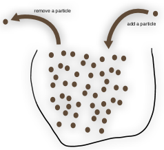
The notation encodes a transition in which i𝑖i copies of a particle of species A𝐴A are transformed into o𝑜o copies of the same species, whileThe SI unit of base rates is in fact [s1]delimited-[]superscript𝑠1[s^{-1}], but we will work throughout with dimensionless units due to the fact that rates are always multiplied by the system’s time parameter t𝑡t in our applications. ri,o0subscript𝑟𝑖𝑜subscriptabsent0r_{i,o}\in\mathbb{R}_{\geq 0} denotes the transition’s base rate. As sketched in Figure 1, one should think of the physical system to consist of a finite number of indistinguishable particles of type A𝐴A, with the transitions implementing operations of removing and adding particles to the system. In this standard description, the positions and impulses of the individual particles are completely neglected, and all physical parameters such as temperature, pressure, volume, chemical potentials etc. are collected into the values of the base rates.
Refer to caption
Fig.  1:  Sketch of the action of the creation operator asuperscript𝑎a^{{\dagger}} (adding a particle) and of the annihilation operator a𝑎a (removing a particle, in all possible ways) on an urn with a precise number n𝑛n of particles (i.e. a pure state |nket𝑛\left|n\right\rangle). See equation (27) below for the concrete definitions.

The precise details of the dynamics of the system include of course the way in which transitions occur. Following the general principles of stochastic mechanics introduced in the previous section, we would like to know how a transition influences the time-dependent state |Ψ(t)ketΨ𝑡\left|\Psi(t)\right\rangle of the system. We identify in the single-species case as pure states configurations with a precise (and finite) number of particles n𝑛n, which we denote by |nket𝑛\left|n\right\rangle. Then according to the general formalism, |Ψ(t)ketΨ𝑡\left|\Psi(t)\right\rangle is a probability distribution over these pure states with time-dependent coefficients ψn(t)subscript𝜓𝑛𝑡\psi_{n}(t),

|Ψ(t)=n0ψn(t)|n.ketΨ𝑡subscript𝑛0subscript𝜓𝑛𝑡ket𝑛\left|\Psi(t)\right\rangle=\sum_{n\geq 0}\psi_{n}(t)\left|n\right\rangle\,. (20)

We quote from the literature (see e.g. [2]) the following result: for a reaction such as in (19) that consumes i𝑖i particles and produces o𝑜o particles at rate ri,osubscript𝑟𝑖𝑜r_{i,o}, the change to the coefficient ψn(t)subscript𝜓𝑛𝑡\psi_{n}(t) in |Ψ(t)ketΨ𝑡\left|\Psi(t)\right\rangle obeys

ddtψn(t)=ri,o((n+io)iψn+io(t)(n)iψn(t)),𝑑𝑑𝑡subscript𝜓𝑛𝑡subscript𝑟𝑖𝑜subscript𝑛𝑖𝑜𝑖subscript𝜓𝑛𝑖𝑜𝑡subscript𝑛𝑖subscript𝜓𝑛𝑡\frac{d}{dt}\psi_{n}(t)=r_{i,o}\bigg{(}(n+i-o)_{i}\psi_{n+i-o}(t)-(n)_{i}\psi_{n}(t)\bigg{)}\,, (21)

where we use the notational conventionWe define Θ(x)Θ𝑥\Theta(x) as (a variant of) the Heaviside step function Θ(x):={1if x00else.assignΘ𝑥cases1if 𝑥00else.\Theta(x):=\begin{cases}1\quad&\text{if }x\geq 0\\ 0\quad&\text{else.}\end{cases}

(n)i:=i!(ni)Θ(ni)n!(ni)!,assignsubscript𝑛𝑖𝑖binomial𝑛𝑖Θ𝑛𝑖𝑛𝑛𝑖(n)_{i}:=i!\binom{n}{i}\equiv\Theta(n-i)\frac{n!}{(n-i)!}\,, (22)

whence (n)i=0subscript𝑛𝑖0(n)_{i}=0 for n<i𝑛𝑖n<i.

Before proceeding with the analysis, it is interesting to note that the coefficient (n)isubscript𝑛𝑖(n)_{i} has in fact a natural combinatorial interpretation: since we consider all particles as indistinguishable, (n)isubscript𝑛𝑖(n)_{i} may be interpreted as the number of ways to pick i𝑖i particles out of a pool of n𝑛n particles without replacement.

As standard in the literature and pioneered by M. Delbrück [1], (21) may be expressed in a more tractable form via the introduction of the concept of probability generating functions: given the formula for the time-dependent state |Ψ(t)ketΨ𝑡\left|\Psi(t)\right\rangle of the system as in (20), one may construct the formal power series P(t;x)𝑃𝑡𝑥P(t;x) (with formal variable x𝑥x):

P(t;x):=n0ψn(t)xn.assign𝑃𝑡𝑥subscript𝑛0subscript𝜓𝑛𝑡superscript𝑥𝑛P(t;x):=\sum_{n\geq 0}\psi_{n}(t)x^{n}\,. (23)

We further introduce the linear operators xsubscript𝑥\partial_{x} and x^^𝑥\hat{x}, defined to act on arbitrary formal power series f(x)𝑓𝑥f(x) according to

xf(x):=xf(x),x^f(x):=xf(x).formulae-sequenceassignsubscript𝑥𝑓𝑥𝑥𝑓𝑥assign^𝑥𝑓𝑥𝑥𝑓𝑥\partial_{x}f(x):=\tfrac{\partial}{\partial x}f(x)\,,\quad\hat{x}f(x):=xf(x)\,. (24)

Since in particular

(x)ixn=(n)ixni,superscriptsubscript𝑥𝑖superscript𝑥𝑛subscript𝑛𝑖superscript𝑥𝑛𝑖\left(\partial_{x}\right)^{i}x^{n}=(n)_{i}\>x^{n-i}\,,

this allows us to recast the information encoded in (21) in the form of an evolution equation for P(t;x)𝑃𝑡𝑥P(t;x):

tP(t;x)=ri,o(x^ox^i)(x)iP(t;x).𝑡𝑃𝑡𝑥subscript𝑟𝑖𝑜superscript^𝑥𝑜superscript^𝑥𝑖superscriptsubscript𝑥𝑖𝑃𝑡𝑥\frac{\partial}{\partial t}P(t;x)=r_{i,o}\big{(}\hat{x}^{o}-\hat{x}^{i}\big{)}\left(\partial_{x}\right)^{i}\>P(t;x)\,. (25)

The readers familiar with the theory of the Heisenberg-Weyl (HW) algebra (see e.g. [10]) will recognize the operators x^^𝑥\hat{x} and xsubscript𝑥\partial_{x} as the generators of the HW algebra in the Bargmann-Fock representation, whose defining relation is computed (for f(x)𝑓𝑥f(x) an arbitrary formal power series) from

[x,x^]f(x)=f(x).subscript𝑥^𝑥𝑓𝑥𝑓𝑥[\partial_{x},\hat{x}]f(x)=f(x)\,. (26)

Contact with the standard notations of stochastic mechanics is made by employing instead the isomorphic so-called canonical representation of the HW algebra, via the one-to-one correspondence

xnsuperscript𝑥𝑛\displaystyle x^{n} |nket𝑛\displaystyle\quad\leftrightarrow\quad\left|n\right\rangle (27)
x^^𝑥\displaystyle\hat{x} asuperscript𝑎\displaystyle\quad\leftrightarrow\quad a^{{\dagger}}
xsubscript𝑥\displaystyle\partial_{x} a,𝑎\displaystyle\quad\leftrightarrow\quad a\,,

with |nket𝑛\left|n\right\rangle the pure state of n𝑛n particles as before. The operator asuperscript𝑎a^{{\dagger}} is called the creation operator and a𝑎a the annihilation operator. One obtains via the one-to-one correspondence (27) the following concrete properties of this representation§§§Note that this particular normalization is sometimes referred to in the literature as the “mathematics variant” [29, 30] of bosons, as opposed to the “physics variant”, in which the normalization is chosen more symmetrically.

a|n=|n+1,a|n=(n)1|n1.formulae-sequencesuperscript𝑎ket𝑛ket𝑛1𝑎ket𝑛subscript𝑛1ket𝑛1a^{{\dagger}}\left|n\right\rangle=\left|n+1\right\rangle\,,\quad a\left|n\right\rangle=(n)_{1}\left|n-1\right\rangle\,. (28)

We are now finally in a position to formulate the Hamiltonian H𝐻H of a chemical reaction system in the form proposed by M. Doi [3]:

Definition 6.

Consider a chemical reaction system of one species, specified in terms of an initial state,

|Ψ(0)=n0ψn(0)|n,ketΨ0subscript𝑛0subscript𝜓𝑛0ket𝑛\left|\Psi(0)\right\rangle=\sum_{n\geq 0}\psi_{n}(0)\left|n\right\rangle,

and a set of one-species reactions,

iAri,ooA.superscriptsubscript𝑟𝑖𝑜𝑖𝐴𝑜𝐴i\>A\stackrel{{\scriptstyle r_{i,o}}}{{\rightharpoonup}}o\>A\,.

Then this data induces a notion of stochastic transition system, namely a continuous-time Markov chain on the space of probability distributions over the number vectors and with infinitesimal generator

H=i,o0ri,o((a)o(a)i)ai.𝐻subscript𝑖𝑜0subscript𝑟𝑖𝑜superscriptsuperscript𝑎𝑜superscriptsuperscript𝑎𝑖superscript𝑎𝑖H=\sum_{i,o\geq 0}r_{i,o}\left(\left(a^{{\dagger}}\right)^{o}-\left(a^{{\dagger}}\right)^{i}\right)a^{i}\,. (29)

We emphasize that i𝑖i and o𝑜o in the above formula take non-negative integer values, such that for example

(a)o=aao times.superscriptsuperscript𝑎𝑜subscriptsuperscript𝑎superscript𝑎o times\left(a^{{\dagger}}\right)^{o}=\underbrace{a^{{\dagger}}\cdots a^{{\dagger}}}_{\text{$o$ times}}\,.

Referring to the standard chemistry literature (see e.g. [2]) for the precise details, in practice only reactions with at most two input or output particles and a total number of at most three particles have to be considered, whence

0i,o2, 1i+o3.formulae-sequence0𝑖formulae-sequence𝑜21𝑖𝑜30\leq i,o\leq 2\,,\;1\leq i+o\leq 3\,.

The corresponding formulae are presented in the first column of Table 1.

Following the stochastic mechanics formalism, it then remains to construct a dual reference state |bra\left\langle\mathcal{R}\right| and to identify observables.

Definition 7.

The dual number vectorsNote that “dual” is to be understood as “formal dual”, i.e. via action on basis vectors; we have to resort to this technicality since 1(S)superscriptsubscript1𝑆\ell_{1}^{\mathbb{R}}(S) does not admit a proper topological dual. m|bra𝑚\left\langle m\right| (for non-negative integers m𝑚m) are defined via their actions on basis vectors,

m|n:=δm,nn!.assigninner-product𝑚𝑛subscript𝛿𝑚𝑛𝑛\left\langle\left.m\right|n\right\rangle:=\delta_{m,n}\>n!\,. (30)

One may then define the resolution of the identity,

𝟙=n01n!|nn|,double-struck-𝟙subscript𝑛01𝑛ket𝑛bra𝑛\mathbb{1}=\sum_{n\geq 0}\frac{1}{n!}\left|n\right\rangle\left\langle n\right|\,, (31)

as well as the concrete realization of the dual reference vector |bra\left\langle\mathcal{R}\right| on the state space spanned by the number vectors,

|n01n!n|=0|ea.brasubscript𝑛01𝑛bra𝑛bra0superscript𝑒𝑎\left\langle\mathcal{R}\right|\equiv\sum_{n\geq 0}\frac{1}{n!}\left\langle n\right|=\left\langle 0\right|e^{a}\,. (32)

We refer the reader to Appendix A.1 for a comparison of these conventions to the analogous concepts in quantum mechanics (and in particular for a comparison of the definition of |bra\left\langle\mathcal{R}\right| to that of coherent states).

The dual reference vector |bra\left\langle\mathcal{R}\right| is thus in particular a left eigenvector with eigenvalue 111 of the creation operator asuperscript𝑎a^{{\dagger}} ,

|a=|,brasuperscript𝑎bra\left\langle\mathcal{R}\right|a^{{\dagger}}=\left\langle\mathcal{R}\right|\,, (33)

which may be seen as follows:

|abrasuperscript𝑎\displaystyle\left\langle\mathcal{R}\right|a^{{\dagger}} =0|eaa=m01m!0|amaabsentbra0superscript𝑒𝑎superscript𝑎subscript𝑚01𝑚bra0superscript𝑎𝑚superscript𝑎\displaystyle=\left\langle 0\right|e^{a}a^{{\dagger}}=\sum_{m\geq 0}\frac{1}{m!}\left\langle 0\right|a^{m}a^{{\dagger}}
=m1(m)1m!0|am1=|.absentsubscript𝑚1subscript𝑚1𝑚bra0superscript𝑎𝑚1bra\displaystyle=\sum_{m\geq 1}\frac{(m)_{1}}{m!}\left\langle 0\right|a^{m-1}=\left\langle\mathcal{R}\right|\,.

It remains finally to identify a realization of observables for single-species chemical reaction systems. It is straightforward to identify the number operator

n^:=aaassign^𝑛superscript𝑎𝑎\hat{n}:=a^{{\dagger}}a (34)

as an observable, since due to

n^|n=n|n^𝑛ket𝑛𝑛ket𝑛\hat{n}\left|n\right\rangle=n\left|n\right\rangle (35)

every pure state |nket𝑛\left|n\right\rangle is an eigenvector of n^^𝑛\hat{n} as required for n^^𝑛\hat{n} to qualify as an observable according to Definition 3. Referring to equation (152) in Appendix A.3 for the precise details, every element of the Heisenberg-Weyl algebra may be expressed as a linear combination of so-called normal-ordered terms arassuperscript𝑎absent𝑟superscript𝑎𝑠a^{{\dagger}\>r}a^{s}. Amongst such terms, there exists a whole family of operators of the form akaksuperscript𝑎absent𝑘superscript𝑎𝑘a^{{\dagger}\>k}a^{k} (with k𝑘k a non-negative integer) that are diagonal in the basis spanned by the vectors |nket𝑛\left|n\right\rangle:

akak|n=(n)k|n.superscript𝑎absent𝑘superscript𝑎𝑘ket𝑛subscript𝑛𝑘ket𝑛a^{{\dagger}\>k}a^{k}\left|n\right\rangle=(n)_{k}\left|n\right\rangle\,. (36)

However, there is an important relationship well-known from the combinatorics literature between powers of n^^𝑛\hat{n} and members of the above family:

Theorem 2.

For arbitrary k,0𝑘subscriptabsent0k,\ell\in\mathbb{Z}_{\geq 0}, we have that

akak==0ks1(k,)n^,n^=k=0S2(,k)akak,formulae-sequencesuperscript𝑎absent𝑘superscript𝑎𝑘superscriptsubscript0𝑘subscript𝑠1𝑘superscript^𝑛superscript^𝑛superscriptsubscript𝑘0subscript𝑆2𝑘superscript𝑎absent𝑘superscript𝑎𝑘a^{{\dagger}\>k}a^{k}=\sum_{\ell=0}^{k}s_{1}(k,\ell)\hat{n}^{\ell}\,,\quad\hat{n}^{\ell}=\sum_{k=0}^{\ell}S_{2}(\ell,k)a^{{\dagger}\>k}a^{k}\,, (37)

where s1(k,)subscript𝑠1𝑘s_{1}(k,\ell) are the Stirling numbers of the first kind, while S2(,k)subscript𝑆2𝑘S_{2}(\ell,k) denotes the Stirling numbers of the second kind (see Appendix B for the explicit definitions).

Proof.

See for example [8]. ∎

What this theorem entails is that for single-species reaction systems we may describe the entire statistics in terms of either the expectation value and higher order moments of the number operator n^^𝑛\hat{n}, or alternatively in terms of the expectation values of the operators akaksuperscript𝑎absent𝑘superscript𝑎𝑘a^{{\dagger}\>k}a^{k}. The latter are referred to in the statistics literature as factorial moments.

With these preparations, it becomes evident that the combinatorics of normal ordering and related techniques can be of use in the study of chemical reaction systems in two main ways: either to explicitly compute the time-dependent state |Ψ(t)ketΨ𝑡\left|\Psi(t)\right\rangle (see Section 6), or alternatively in order to formulate and solve evolution equations for observable generating functions. The former can be accomplished in a concise way:

Theorem 3.

Given a one-species chemical reaction system according to Definition 6, the exponential moment generating function (t;λ)𝑡𝜆\mathcal{M}(t;\lambda) of the number operator n^^𝑛\hat{n},

(t;λ):=|eλn^|Ψ(t),assign𝑡𝜆quantum-operator-productsuperscript𝑒𝜆^𝑛Ψ𝑡\mathcal{M}(t;\lambda):=\left.\left\langle\mathcal{R}\left|e^{\lambda\hat{n}}\right|\Psi(t)\right\rangle\right.\,, (38)

fulfills the evolution equation

t(t;λ)𝑡𝑡𝜆\displaystyle\tfrac{\partial}{\partial t}\mathcal{M}(t;\lambda) =𝔻(λ,λ)(t;λ)absent𝔻𝜆subscript𝜆𝑡𝜆\displaystyle=\mathbb{D}(\lambda,\partial_{\lambda})\mathcal{M}(t;\lambda) (39)
𝔻(λ,λ)𝔻𝜆subscript𝜆\displaystyle\mathbb{D}(\lambda,\partial_{\lambda}) =i,ori,o𝔻(i,o)absentsubscript𝑖𝑜subscript𝑟𝑖𝑜subscript𝔻𝑖𝑜\displaystyle=\sum_{i,o}r_{i,o}\mathbb{D}_{(i,o)}
𝔻(i,o)subscript𝔻𝑖𝑜\displaystyle\mathbb{D}_{(i,o)} =(eλ(oi)1)=0is1(i,)(λ).absentsuperscript𝑒𝜆𝑜𝑖1superscriptsubscript0𝑖subscript𝑠1𝑖superscript𝜆\displaystyle=\left(e^{\lambda(o-i)}-1\right)\sum_{\ell=0}^{i}s_{1}(i,\ell)\left(\tfrac{\partial}{\partial\lambda}\right)^{\ell}\,.
Proof.

See Appendix C.2

Another interesting variant of generating function evolution equations is provided upon considering the factorial moment generating function (t;ν)𝑡𝜈\mathcal{F}(t;\nu), defined as

(t;ν):=n0νnn!|anan|Ψ(t).assign𝑡𝜈subscript𝑛0superscript𝜈𝑛𝑛quantum-operator-productsuperscript𝑎absent𝑛superscript𝑎𝑛Ψ𝑡\mathcal{F}(t;\nu):=\sum_{n\geq 0}\frac{\nu^{n}}{n!}\left.\left\langle\mathcal{R}\left|a^{{\dagger}\>n}a^{n}\right|\Psi(t)\right\rangle\right.\,. (40)

Because the operation ||Ψ(t)quantum-operator-productΨ𝑡\left\langle\mathcal{R}\right|\dotsc\left|\Psi(t)\right\rangle of taking the expectation value in the state |Ψ(t)ketΨ𝑡\left|\Psi(t)\right\rangle is linear in its argument, (t;ν)𝑡𝜈\mathcal{F}(t;\nu) may be seen as a kind of “change of basis” for the observables of the stochastic system, i.e. from moments of the number operator to factorial moments.

Theorem 4.

The generating function (t;ν)𝑡𝜈\mathcal{F}(t;\nu) obeys the following evolution equation:

t(t;ν)𝑡𝑡𝜈\displaystyle\tfrac{\partial}{\partial t}\mathcal{F}(t;\nu) =𝕕(ν,ν)(t;ν)absent𝕕𝜈subscript𝜈𝑡𝜈\displaystyle=\mathbb{d}(\nu,\partial_{\nu})\mathcal{F}(t;\nu) (41)
𝕕(ν,ν)𝕕𝜈subscript𝜈\displaystyle\mathbb{d}(\nu,\partial_{\nu}) =i,ori,o𝕕(i,o)absentsubscript𝑖𝑜subscript𝑟𝑖𝑜subscript𝕕𝑖𝑜\displaystyle=\sum_{i,o}r_{i,o}\mathbb{d}_{(i,o)}
𝕕(i,o)subscript𝕕𝑖𝑜\displaystyle\mathbb{d}_{(i,o)} =((ν+1)o(ν+1)i)(ν)i.absentsuperscript𝜈1𝑜superscript𝜈1𝑖superscript𝜈𝑖\displaystyle=\left((\nu+1)^{o}-(\nu+1)^{i}\right)\left(\tfrac{\partial}{\partial\nu}\right)^{i}\,.
Proof.

See Appendix C.3

In summary, chemical reaction systems of one species may be described equivalently in terms of either of the three formulae:

  • (i)

    the explicit formula for the probability distribution,

    |Ψ(t)=(t)|Ψ(0),ketΨ𝑡𝑡ketΨ0\left|\Psi(t)\right\rangle=\mathcal{E}(t)\left|\Psi(0)\right\rangle\,,
  • (ii)

    the evolution equation for the exponential moment generating function (t;λ)𝑡𝜆\mathcal{M}(t;\lambda) of the number operator n^^𝑛\hat{n},

    t(t;λ)=𝔻(λ,λ)(t;λ),𝑡𝑡𝜆𝔻𝜆subscript𝜆𝑡𝜆\tfrac{\partial}{\partial t}\mathcal{M}(t;\lambda)=\mathbb{D}(\lambda,\partial_{\lambda})\mathcal{M}(t;\lambda)\,,
  • (iii)

    the evolution equation for the factorial moment generating function (t;ν)𝑡𝜈\mathcal{F}(t;\nu),

    t(t;ν)=𝕕(ν,ν)(t;ν).𝑡𝑡𝜈𝕕𝜈subscript𝜈𝑡𝜈\tfrac{\partial}{\partial t}\mathcal{F}(t;\nu)=\mathbb{d}(\nu,\partial_{\nu})\mathcal{F}(t;\nu)\,.

We summarize the explicit formulae for individual transitions iAri,ooAsuperscriptsubscript𝑟𝑖𝑜𝑖𝐴𝑜𝐴i\>A\stackrel{{\scriptstyle r_{i,o}}}{{\rightharpoonup}}o\>A in Table 1, both for generic transitions and for the ones of empirical relevance in the theory of chemical reaction systems (cf. the remarks after equation (29)).

Table 1:  Contributions H(i,o)subscript𝐻𝑖𝑜H_{(i,o)} to the evolution operator H𝐻H (cf. (29)), 𝔻(i,o)subscript𝔻𝑖𝑜\mathbb{D}_{(i,o)} to the differential operator 𝔻𝔻(λ,λ)𝔻𝔻𝜆subscript𝜆\mathbb{D}\equiv\mathbb{D}(\lambda,\partial_{\lambda}) (cf. (39)) and 𝕕(i,o)subscript𝕕𝑖𝑜\mathbb{d}_{(i,o)} to 𝕕𝕕(ν,ν)𝕕𝕕𝜈subscript𝜈\mathbb{d}\equiv\mathbb{d}(\nu,\partial_{\nu}) (cf. (41)) of individual chemical reactions iAri,ooAsubscript𝑟𝑖𝑜𝑖𝐴𝑜𝐴i\>A\xrightharpoonup{\;r_{i,o}\;}o\>A
Parameters H(i,o)subscript𝐻𝑖𝑜H_{(i,o)} 𝔻(i,o)subscript𝔻𝑖𝑜\mathbb{D}_{(i,o)} 𝕕(i,o)subscript𝕕𝑖𝑜\mathbb{d}_{(i,o)}
(i,o)𝑖𝑜(i,o) ri,o(aoai)aisubscript𝑟𝑖𝑜superscript𝑎absent𝑜superscript𝑎absent𝑖superscript𝑎𝑖r_{i,o}\left(a^{{\dagger}\>o}-a^{{\dagger}\>i}\right)a^{i} ri,o(eλ(oi)1)=0is1(i,)(λ)subscript𝑟𝑖𝑜superscript𝑒𝜆𝑜𝑖1superscriptsubscript0𝑖subscript𝑠1𝑖superscript𝜆r_{i,o}\left(e^{\lambda(o-i)}-1\right)\sum_{\ell=0}^{i}s_{1}(i,\ell)\left(\tfrac{\partial}{\partial\lambda}\right)^{\ell} ri,o((ν+1)o(ν+1)i)(ν)isubscript𝑟𝑖𝑜superscript𝜈1𝑜superscript𝜈1𝑖superscript𝜈𝑖r_{i,o}\left((\nu+1)^{o}-(\nu+1)^{i}\right)\left(\tfrac{\partial}{\partial\nu}\right)^{i}
(0,2)02(0,2) r0,2(a 21)subscript𝑟02superscript𝑎absent21r_{0,2}\left(a^{{\dagger}\>2}-1\right) r0,2(e2λ1)subscript𝑟02superscript𝑒2𝜆1r_{0,2}\left(e^{2\lambda}-1\right) r0,2(ν2+2ν)subscript𝑟02superscript𝜈22𝜈r_{0,2}\left(\nu^{2}+2\nu\right)
(0,1)01(0,1) r0,1(a1)subscript𝑟01superscript𝑎1r_{0,1}(a^{{\dagger}}-1) r0,1(eλ1)subscript𝑟01superscript𝑒𝜆1r_{0,1}\left(e^{\lambda}-1\right) r0,1νsubscript𝑟01𝜈r_{0,1}\nu
(1,2)12(1,2) r1,2(a 2a)asubscript𝑟12superscript𝑎absent2superscript𝑎𝑎r_{1,2}\left(a^{{\dagger}\>2}-a^{{\dagger}}\right)a r1,2(eλ1)λsubscript𝑟12superscript𝑒𝜆1𝜆r_{1,2}\left(e^{\lambda}-1\right)\frac{\partial}{\partial\lambda} r1,2(ν2+ν)νsubscript𝑟12superscript𝜈2𝜈𝜈r_{1,2}(\nu^{2}+\nu)\frac{\partial}{\partial\nu}
(1,0)10(1,0) r1,0(1a)asubscript𝑟101superscript𝑎𝑎r_{1,0}\left(1-a^{{\dagger}}\right)a r1,0(eλ1)λλsubscript𝑟10superscript𝑒𝜆1𝜆𝜆r_{1,0}\left(e^{-\lambda}-1\right)\frac{\lambda}{\partial\lambda} r1,0ννsubscript𝑟10𝜈𝜈-r_{1,0}\nu\frac{\partial}{\partial\nu}
(2,1)21(2,1) r2,1(aa 2)a2subscript𝑟21superscript𝑎superscript𝑎absent2superscript𝑎2r_{2,1}\left(a^{{\dagger}}-a^{{\dagger}\>2}\right)a^{2} r2,1(eλ1)(2λ2λ)subscript𝑟21superscript𝑒𝜆1superscript2superscript𝜆2𝜆r_{2,1}\left(e^{-\lambda}-1\right)\left(\frac{\partial^{2}}{\partial\lambda^{2}}-\frac{\partial}{\partial\lambda}\right) r2,1(ν2+ν)2ν2subscript𝑟21superscript𝜈2𝜈superscript2superscript𝜈2-r_{2,1}(\nu^{2}+\nu)\frac{\partial^{2}}{\partial\nu^{2}}
(2,0)20(2,0) r2,0(1a 2)a2subscript𝑟201superscript𝑎absent2superscript𝑎2r_{2,0}\left(1-a^{{\dagger}\>2}\right)a^{2} r2,0(e2λ1)(2λ2λ)subscript𝑟20superscript𝑒2𝜆1superscript2superscript𝜆2𝜆r_{2,0}\left(e^{-2\lambda}-1\right)\left(\frac{\partial^{2}}{\partial\lambda^{2}}-\frac{\partial}{\partial\lambda}\right) r2,0(ν2+2ν)2ν2subscript𝑟20superscript𝜈22𝜈superscript2superscript𝜈2-r_{2,0}(\nu^{2}+2\nu)\frac{\partial^{2}}{\partial\nu^{2}}

4 Multi-species reaction systems

The key ingredient will be the canonical representation of the multi-species Heisenberg-Weyl (HW) algebra (over the real numbers):

Definition 8.

Let 𝐒𝐒\mathbf{S} be a set of species (i.e. in general a denumerable set). Define a set of basis vectors

|n¯|ni1,ni2,,ket¯𝑛ketsubscript𝑛subscript𝑖1subscript𝑛subscript𝑖2\left|\underline{n}\right\rangle\equiv\left|n_{i_{1}},n_{i_{2}},\dotsc\right\rangle\,, (42)

called the multi-species number vectors. Since each of these vectors will be interpreted to represent a pure state, whence a realizable configuration of the system, we require in addition that all nisubscript𝑛𝑖n_{i} must be non-negative integers, and that only finitely many of the nisubscript𝑛𝑖n_{i} are non-zero. Then the canonical representation of the multi-species Heisenberg-Weyl algebra is defined via

ai|n¯superscriptsubscript𝑎𝑖ket¯𝑛\displaystyle a_{i}^{{\dagger}}\left|\underline{n}\right\rangle :=|n¯+Δ¯iassignabsentket¯𝑛subscript¯Δ𝑖\displaystyle:=\left|\underline{n}+\underline{\Delta}_{i}\right\rangle (43)
aj|n¯subscript𝑎𝑗ket¯𝑛\displaystyle a_{j}\left|\underline{n}\right\rangle :=(nj)1|n¯Δ¯j,assignabsentsubscriptsubscript𝑛𝑗1ket¯𝑛subscript¯Δ𝑗\displaystyle:=(n_{j})_{1}\left|\underline{n}-\underline{\Delta}_{j}\right\rangle\,,

with (nj)1subscriptsubscript𝑛𝑗1(n_{j})_{1} denoting the falling factorials

(nj)1=Θ(nj1)(nj)!(nj1)!.subscriptsubscript𝑛𝑗1Θsubscript𝑛𝑗1subscript𝑛𝑗subscript𝑛𝑗1(n_{j})_{1}=\Theta(n_{j}-1)\frac{(n_{j})!}{(n_{j}-1)!}\,.

We have moreover introduced the convenient shorthand notation Δ¯isubscript¯Δ𝑖\underline{\Delta}_{i} for a vector of non-negative integers whose only non-zero coordinate is ni=1subscript𝑛𝑖1n_{i}=1.

The fact that these linear operators foster a representation of the multi-species HW algebra is confirmed by noting that the following canonical commutation relationsMore precisely, each of the relations in (44) is an equation on linear operators, whose validity may be verified by acting on generic basis vectors |n¯ket¯𝑛\left|\underline{n}\right\rangle. hold true:

[ai,aj]=δi,j,[ai,aj]=0=[ai,aj].formulae-sequencesubscript𝑎𝑖subscriptsuperscript𝑎𝑗subscript𝛿𝑖𝑗subscript𝑎𝑖subscript𝑎𝑗0superscriptsubscript𝑎𝑖superscriptsubscript𝑎𝑗[a_{i},a^{{\dagger}}_{j}]=\delta_{i,j}\,,\quad[a_{i},a_{j}]=0=[a_{i}^{{\dagger}},a_{j}^{{\dagger}}]\,. (44)

The following additional multi-index notations will prove convenient throughout this section:

n¯!¯𝑛\displaystyle\underline{n}! i𝐒(ni)!,x¯y¯i𝐒(xiyi),ex¯i𝐒exiformulae-sequenceabsentsubscriptproduct𝑖𝐒subscript𝑛𝑖formulae-sequencesuperscript¯𝑥¯𝑦subscriptproduct𝑖𝐒superscriptsubscript𝑥𝑖subscript𝑦𝑖superscript𝑒¯𝑥subscriptproduct𝑖𝐒superscript𝑒subscript𝑥𝑖\displaystyle\equiv\prod_{i\in\mathbf{S}}(n_{i})!\,,\;\underline{x}^{\underline{y}}\equiv\prod_{i\in\mathbf{S}}\left(x_{i}^{y_{i}}\right)\,,\;e^{\underline{x}}\equiv\prod_{i\in\mathbf{S}}e^{x_{i}} (45)
(m¯)n¯subscript¯𝑚¯𝑛\displaystyle(\underline{m})_{\underline{n}} i𝐒((mi)ni):=i𝐒((mi)!(mini)!)absentsubscriptproduct𝑖𝐒subscriptsubscript𝑚𝑖subscript𝑛𝑖assignsubscriptproduct𝑖𝐒subscript𝑚𝑖subscript𝑚𝑖subscript𝑛𝑖\displaystyle\equiv\prod_{i\in\mathbf{S}}\left((m_{i})_{n_{i}}\right):=\prod_{i\in\mathbf{S}}\left(\frac{(m_{i})!}{(m_{i}-n_{i})!}\right)
(m¯n¯)binomial¯𝑚¯𝑛\displaystyle\binom{\underline{m}}{\underline{n}} =i𝐒(mini),δm¯,n¯i𝐒δmi,ni.formulae-sequenceabsentsubscriptproduct𝑖𝐒binomialsubscript𝑚𝑖subscript𝑛𝑖subscript𝛿¯𝑚¯𝑛subscriptproduct𝑖𝐒subscript𝛿subscript𝑚𝑖subscript𝑛𝑖\displaystyle=\prod_{i\in\mathbf{S}}\binom{m_{i}}{n_{i}}\,,\;\delta_{\underline{m},\underline{n}}\equiv\prod_{i\in\mathbf{S}}\delta_{m_{i},n_{i}}\,.

An immediate consequence of (44) is that we can express any element of the multi-species HW algebra in terms of linear combinations of normal-ordered expressions of the form a¯r¯a¯s¯superscript¯𝑎absent¯𝑟superscript¯𝑎¯𝑠\underline{a}^{{\dagger}\>\underline{r}}\underline{a}^{\underline{s}} (with r¯,s¯¯𝑟¯𝑠\underline{r},\underline{s} vectors of non-negative integers), which is a consequence of the well-known normal ordering formula (cf. e.g. [8])

a¯m¯a¯n¯a¯r¯a¯s¯=k¯0¯k¯!(n¯k¯)(r¯k¯)a¯(m¯+r¯k¯)a¯(n¯+s¯k¯).superscript¯𝑎absent¯𝑚superscript¯𝑎¯𝑛superscript¯𝑎absent¯𝑟superscript¯𝑎¯𝑠subscript¯𝑘¯0¯𝑘binomial¯𝑛¯𝑘binomial¯𝑟¯𝑘superscript¯𝑎absent¯𝑚¯𝑟¯𝑘superscript¯𝑎¯𝑛¯𝑠¯𝑘\displaystyle\underline{a}^{{\dagger}\>\underline{m}}\underline{a}^{\underline{n}}\underline{a}^{{\dagger}\>\underline{r}}\underline{a}^{\underline{s}}=\sum_{\underline{k}\geq\underline{0}}\underline{k}!\binom{\underline{n}}{\underline{k}}\binom{\underline{r}}{\underline{k}}\underline{a}^{{\dagger}\>(\underline{m}+\underline{r}-\underline{k})}\underline{a}^{(\underline{n}+\underline{s}-\underline{k})}\,. (46)

Here, we have made use of the standard convention (xy)=0binomial𝑥𝑦0\binom{x}{y}=0 whenever y>x𝑦𝑥y>x.

We will use the following normalization for the (formal) dual vectors m¯|bra¯𝑚\left\langle\underline{m}\right|:

m¯|n¯:=n¯!δm¯,n¯.assigninner-product¯𝑚¯𝑛¯𝑛𝛿¯𝑚¯𝑛\left\langle\left.\underline{m}\right|\underline{n}\right\rangle:=\underline{n}!\delta{\underline{m},\underline{n}}\,. (47)

The multi-species version ¯|bra¯\left\langle\underline{\mathcal{R}}\right| of the reference dual vector is defined as

¯|:=m¯0¯1m¯!m¯|.assignbra¯subscript¯𝑚¯01¯𝑚bra¯𝑚\left\langle\underline{\mathcal{R}}\right|:=\sum_{\underline{m}\geq\underline{0}}\frac{1}{\underline{m}!}\left\langle\underline{m}\right|\,. (48)

With the relations

|n¯=a¯n¯|0¯,m¯|=(a¯m¯|0¯)=0¯|a¯m¯,formulae-sequenceket¯𝑛superscript¯𝑎absent¯𝑛ket¯0bra¯𝑚superscriptsuperscript¯𝑎¯𝑚ket¯0bra¯0superscript¯𝑎¯𝑚\left|\underline{n}\right\rangle=\underline{a}^{{\dagger}\>\underline{n}}\left|\underline{0}\right\rangle\,,\;\left\langle\underline{m}\right|=\left(\underline{a}^{\underline{m}}\left|\underline{0}\right\rangle\right)^{{\dagger}}=\left\langle\underline{0}\right|\underline{a}^{\underline{m}}\,, (49)

which are compatible with m¯|n¯=n¯!δm¯,n¯inner-product¯𝑚¯𝑛¯𝑛subscript𝛿¯𝑚¯𝑛\left\langle\left.\underline{m}\right|\underline{n}\right\rangle=\underline{n}!\>\delta_{\underline{m},\underline{n}}, we may identify ¯|bra¯\left\langle\underline{\mathcal{R}}\right| as a simultaneous left eigenvector of the creation operators aisubscriptsuperscript𝑎𝑖a^{{\dagger}}_{i} (i𝐒𝑖𝐒i\in\mathbf{S}) of eigenvalue 111:

¯|ai=0¯|ea¯ai=0¯|(ai+1)ea¯=¯|.bra¯superscriptsubscript𝑎𝑖bra¯0superscript𝑒¯𝑎superscriptsubscript𝑎𝑖bra¯0superscriptsubscript𝑎𝑖1superscript𝑒¯𝑎bra¯\left\langle\underline{\mathcal{R}}\right|a_{i}^{{\dagger}}=\left\langle\underline{0}\right|e^{\underline{a}}a_{i}^{{\dagger}}=\left\langle\underline{0}\right|(a_{i}^{{\dagger}}+1)e^{\underline{a}}=\left\langle\underline{\mathcal{R}}\right|\,. (50)

Here, we have made use of the following very useful general formula (which played a pivotal role in the derivation of several analytical combinatorics formulae, see Section 6):

Proposition 1.

For all real vectors α¯,β¯¯𝛼¯𝛽\underline{\alpha},\underline{\beta}, and for all Taylor-expandable functions f(a¯,a¯)𝑓superscript¯𝑎¯𝑎f(\underline{a}^{{\dagger}},\underline{a}), we have that

eα¯a¯f(a¯,a¯)eβ¯a¯=eα¯β¯eβ¯a¯f(a¯+α¯,a¯+β¯)eα¯a¯.superscript𝑒¯𝛼¯𝑎𝑓superscript¯𝑎¯𝑎superscript𝑒¯𝛽superscript¯𝑎superscript𝑒¯𝛼¯𝛽superscript𝑒¯𝛽superscript¯𝑎𝑓superscript¯𝑎¯𝛼¯𝑎¯𝛽superscript𝑒¯𝛼¯𝑎e^{\underline{\alpha}\cdot\underline{a}}f(\underline{a}^{{\dagger}},\underline{a})e^{\underline{\beta}\cdot\underline{a}^{{\dagger}}}=e^{\underline{\alpha}\cdot\underline{\beta}}e^{\underline{\beta}\cdot\underline{a}^{{\dagger}}}f\left(\underline{a}^{{\dagger}}+\underline{\alpha},\underline{a}+\underline{\beta}\right)e^{\underline{\alpha}\cdot\underline{a}}\,. (51)
Proof.

See Appendix C.4. ∎

Noticing that the multi-species number vectors are simultaneous eigenstates of the number operators n^i:=aiaiassignsubscript^𝑛𝑖superscriptsubscript𝑎𝑖subscript𝑎𝑖\hat{n}_{i}:=a_{i}^{{\dagger}}a_{i} (i𝐒𝑖𝐒i\in\mathbf{S}),

n^i|n¯=(ni)1|n¯,subscript^𝑛𝑖ket¯𝑛subscriptsubscript𝑛𝑖1ket¯𝑛\hat{n}_{i}\left|\underline{n}\right\rangle=(n_{i})_{1}\left|\underline{n}\right\rangle\,, (52)

we have all preparations in place to state the multi-species generalization of the stochastic mechanics framework for chemical reaction systems:

Definition 9.

Consider a chemical reaction system with reactions of the form

i¯A¯ri¯,o¯o¯A¯,subscript𝑟¯𝑖¯𝑜¯𝑖¯𝐴¯𝑜¯𝐴\underline{i}\cdot\underline{A}\xrightharpoonup{\;r_{\underline{i},\underline{o}}\;}\underline{o}\cdot\underline{A}\,, (53)

where i¯,o¯¯𝑖¯𝑜\underline{i},\underline{o} are vectors of non-negative integers (encoding the numbers of particles of each type on input and output of the transition, respectively), and with the reaction rates******We use this convention in order to be able to specify a compact formula for H𝐻H, i.e. only the reactions for parameter pairs (i¯,o¯)¯𝑖¯𝑜(\underline{i},\underline{o}) for ri¯,o¯>0subscript𝑟¯𝑖¯𝑜0r_{\underline{i},\underline{o}}>0 contribute to H𝐻H. ri¯,o¯0subscript𝑟¯𝑖¯𝑜subscriptabsent0r_{\underline{i},\underline{o}}\in\mathbb{R}_{\geq 0}. Then together with an input state

|Ψ(0)Prob(𝒩)ketΨ0𝑃𝑟𝑜𝑏𝒩\left|\Psi(0)\right\rangle\in Prob(\mathcal{N}) (54)

over the state space 𝒩𝒩\mathcal{N} of multi-species number vectors,

Prob(𝒩)|Ψ(0)n¯0¯ψn¯(0)|n¯,contains𝑃𝑟𝑜𝑏𝒩ketΨ0subscript¯𝑛¯0subscript𝜓¯𝑛0ket¯𝑛Prob(\mathcal{N})\ni\left|\Psi(0)\right\rangle\equiv\sum_{\underline{n}\geq\underline{0}}\psi_{\underline{n}}(0)\left|\underline{n}\right\rangle\,, (55)

this data specifies a continuous-time Markov chain with evolution operator

H:=i¯,o¯0¯ri¯,o¯((a¯)o¯(a¯)i¯)a¯i¯.assign𝐻subscript¯𝑖¯𝑜¯0subscript𝑟¯𝑖¯𝑜superscriptsuperscript¯𝑎¯𝑜superscriptsuperscript¯𝑎¯𝑖superscript¯𝑎¯𝑖H:=\sum_{\underline{i},\underline{o}\geq\underline{0}}r_{\underline{i},\underline{o}}\left(\left(\underline{a}^{{\dagger}}\right)^{\underline{o}}-\left(\underline{a}^{{\dagger}}\right)^{\underline{i}}\right)\underline{a}^{\underline{i}}\,. (56)

The main general result on the dynamics of generic chemical reaction systems are the following two generalizations of the moment and factorial moment generating function evolution equations from the previous section. As in the single-species setting, knowing all eigenvalues nisubscript𝑛𝑖n_{i} of a given pure state |n¯ket¯𝑛\left|\underline{n}\right\rangle completely characterizes the eigenstate, such that the moments of the number operators n^isubscript^𝑛𝑖\hat{n}_{i} or the respective factorial moments are providing equivalent knowledge about a system state |Ψ(t)ketΨ𝑡\left|\Psi(t)\right\rangle as the probability distribution itself:

Theorem 5.

For a multi-species chemical reaction system as specified in Definition 9, let the exponential moment generating function (t;λ¯)𝑡¯𝜆\mathcal{M}(t;\underline{\lambda}) of the number operators n^isubscript^𝑛𝑖\hat{n}_{i} and the factorial moment generating function (t;ν¯)𝑡¯𝜈\mathcal{F}(t;\underline{\nu}) be defined as

(t;λ¯)𝑡¯𝜆\displaystyle\mathcal{M}(t;\underline{\lambda}) :=¯|eλ¯n¯^|Ψ(t)assignabsentquantum-operator-product¯superscript𝑒¯𝜆¯^𝑛Ψ𝑡\displaystyle:=\left.\left\langle\underline{\mathcal{R}}\left|e^{\underline{\lambda}\cdot\underline{\hat{n}}}\right|\Psi(t)\right\rangle\right. (57)
(t;ν¯)𝑡¯𝜈\displaystyle\mathcal{F}(t;\underline{\nu}) :=k¯0¯ν¯k¯n¯!¯|a¯k¯a¯k¯|Ψ(t).assignabsentsubscript¯𝑘¯0superscript¯𝜈¯𝑘¯𝑛quantum-operator-product¯superscript¯𝑎absent¯𝑘superscript¯𝑎¯𝑘Ψ𝑡\displaystyle:=\sum_{\underline{k}\geq\underline{0}}\frac{\underline{\nu}^{\underline{k}}}{\underline{n}!}\left.\left\langle\underline{\mathcal{R}}\left|\underline{a}^{{\dagger}\>\underline{k}}\underline{a}^{\underline{k}}\right|\Psi(t)\right\rangle\right.\,.

Then the generating functions satisfy the evolution equations

t(t;λ¯)𝑡𝑡¯𝜆\displaystyle\tfrac{\partial}{\partial t}\mathcal{M}(t;\underline{\lambda}) =𝔻(λ¯,λ¯)(t;λ¯)absent𝔻¯𝜆subscript¯𝜆𝑡¯𝜆\displaystyle=\mathbb{D}(\underline{\lambda},\partial_{\underline{\lambda}})\mathcal{M}(t;\underline{\lambda}) (58)
𝔻(λ¯,λ¯)𝔻¯𝜆subscript¯𝜆\displaystyle\mathbb{D}(\underline{\lambda},\partial_{\underline{\lambda}}) =i¯,o¯𝔻(i¯,o¯)absentsubscript¯𝑖¯𝑜subscript𝔻¯𝑖¯𝑜\displaystyle=\sum_{\underline{i},\underline{o}}\mathbb{D}_{(\underline{i},\underline{o})}
𝔻(i¯,o¯)subscript𝔻¯𝑖¯𝑜\displaystyle\mathbb{D}_{(\underline{i},\underline{o})} =ri¯,o¯(eλ¯(o¯i¯)1)\displaystyle=r_{\underline{i},\underline{o}}\left(e^{\underline{\lambda}\cdot(\underline{o}-\underline{i})}-1\right)\cdot
k¯=0¯i¯s¯1(i¯,k¯)(λ¯)k¯\displaystyle\quad\qquad\cdot\sum_{\underline{k}=\underline{0}}^{\underline{i}}\underline{s}_{1}(\underline{i},\underline{k})\left(\tfrac{\partial}{\partial\underline{\lambda}}\right)^{\underline{k}}
s¯1(i¯,k¯)subscript¯𝑠1¯𝑖¯𝑘\displaystyle\underline{s}_{1}(\underline{i},\underline{k}) :=j𝐒s1(ij,kj),assignabsentsubscriptproduct𝑗𝐒subscript𝑠1subscript𝑖𝑗subscript𝑘𝑗\displaystyle:=\prod_{j\in\mathbf{S}}s_{1}(i_{j},k_{j})\,,

with s1(i,j)subscript𝑠1𝑖𝑗s_{1}(i,j) denoting the Stirling numbers of the first kind, and

t(t;ν¯)𝑡𝑡¯𝜈\displaystyle\tfrac{\partial}{\partial t}\mathcal{F}(t;\underline{\nu}) =𝕕(ν¯,ν¯)(t;ν¯)absent𝕕¯𝜈subscript¯𝜈𝑡¯𝜈\displaystyle=\mathbb{d}(\underline{\nu},\partial_{\underline{\nu}})\mathcal{F}(t;\underline{\nu}) (59)
𝕕(ν¯,ν¯)𝕕¯𝜈subscript¯𝜈\displaystyle\mathbb{d}(\underline{\nu},\partial_{\underline{\nu}}) =i¯,o¯𝕕(i¯,o¯)absentsubscript¯𝑖¯𝑜subscript𝕕¯𝑖¯𝑜\displaystyle=\sum_{\underline{i},\underline{o}}\mathbb{d}_{(\underline{i},\underline{o})}
𝕕(i¯,o¯)subscript𝕕¯𝑖¯𝑜\displaystyle\mathbb{d}_{(\underline{i},\underline{o})} =ri¯,o¯((ν¯+1¯)o¯(ν¯+1¯)i¯)(ν¯)i¯.absentsubscript𝑟¯𝑖¯𝑜superscript¯𝜈¯1¯𝑜superscript¯𝜈¯1¯𝑖superscript¯𝜈¯𝑖\displaystyle=r_{\underline{i},\underline{o}}\left((\underline{\nu}+\underline{1})^{\underline{o}}-(\underline{\nu}+\underline{1})^{\underline{i}}\right)\left(\tfrac{\partial}{\partial\underline{\nu}}\right)^{\underline{i}}\,.
Proof.

See Appendix C.5. ∎

We summarize both these statements as well as explicit formulae for all chemical reactions of practical interest (i.e. for transitions with 1j𝐒(ij+oj)31subscript𝑗𝐒subscript𝑖𝑗subscript𝑜𝑗31\leq\sum_{j\in\mathbf{S}}(i_{j}+o_{j})\leq 3) in Table 2.

Table 2:  Contributions H(i¯,o¯)subscript𝐻¯𝑖¯𝑜H_{(\underline{i},\underline{o})} to the evolution operator H𝐻H (cf. (56)), 𝔻(i¯,o¯)subscript𝔻¯𝑖¯𝑜\mathbb{D}_{(\underline{i},\underline{o})} to the differential operator 𝔻𝔻(λ¯,λ¯)𝔻𝔻¯𝜆subscript¯𝜆\mathbb{D}\equiv\mathbb{D}(\underline{\lambda},\partial_{\underline{\lambda}}) (cf. (58)) and 𝕕(i¯,o¯)subscript𝕕¯𝑖¯𝑜\mathbb{d}_{(\underline{i},\underline{o})} to 𝕕𝕕(ν¯,ν¯)𝕕𝕕¯𝜈subscript¯𝜈\mathbb{d}\equiv\mathbb{d}(\underline{\nu},\partial_{\underline{\nu}}) (cf. (59)) of individual multi-species chemical reactions i¯A¯ri¯,o¯o¯A¯subscript𝑟¯𝑖¯𝑜¯𝑖¯𝐴¯𝑜¯𝐴\underline{i}\cdot\underline{A}\xrightharpoonup{\;r_{\underline{i},\underline{o}}\;}\underline{o}\cdot\underline{A}; concrete values for i¯¯𝑖\underline{i} and o¯¯𝑜\underline{o} are encoded using the notation Δ¯αsubscript¯Δ𝛼\underline{\Delta}_{\alpha} for the vector with all entries equal to zero, except for the α𝛼\alpha-th entry, which is 111 (i.e. Δ¯αsubscript¯Δ𝛼\underline{\Delta}_{\alpha} is the α𝛼\alpha-th unit basis vector)
Parameters H(i¯,o¯)/ri¯,o¯subscript𝐻¯𝑖¯𝑜subscript𝑟¯𝑖¯𝑜H_{(\underline{i},\underline{o})}/r_{\underline{i},\underline{o}} 𝔻(i¯,o¯)/ri¯,o¯subscript𝔻¯𝑖¯𝑜subscript𝑟¯𝑖¯𝑜\mathbb{D}_{(\underline{i},\underline{o})}/r_{\underline{i},\underline{o}} 𝕕(i¯,o¯)/ri¯,o¯subscript𝕕¯𝑖¯𝑜subscript𝑟¯𝑖¯𝑜\mathbb{d}_{(\underline{i},\underline{o})}/r_{\underline{i},\underline{o}}
(o¯,i¯)¯𝑜¯𝑖(\underline{o},\underline{i}) (a¯o¯a¯i¯)a¯i¯superscript¯𝑎absent¯𝑜superscript¯𝑎absent¯𝑖superscript¯𝑎¯𝑖\left(\underline{a}^{{\dagger}\>\underline{o}}-\underline{a}^{{\dagger}\>\underline{i}}\right)\underline{a}^{\underline{i}} (eλ¯(o¯i¯)1)¯=0¯i¯s¯1(i¯,¯)(λ¯)¯superscript𝑒¯𝜆¯𝑜¯𝑖1superscriptsubscript¯¯0¯𝑖subscript¯𝑠1¯𝑖¯superscript¯𝜆¯\left(e^{\underline{\lambda}\cdot(\underline{o}-\underline{i})}-1\right)\sum_{\underline{\ell}=\underline{0}}^{\underline{i}}\underline{s}_{1}(\underline{i},\underline{\ell})\left(\frac{\partial}{\partial\underline{\lambda}}\right)^{\underline{\ell}} ((ν¯+1¯)o¯(ν¯+1¯)i¯)(ν¯)i¯superscript¯𝜈¯1¯𝑜superscript¯𝜈¯1¯𝑖superscript¯𝜈¯𝑖\left((\underline{\nu}+\underline{1})^{\underline{o}}-(\underline{\nu}+\underline{1})^{\underline{i}}\right)\left(\frac{\partial}{\partial\underline{\nu}}\right)^{\underline{i}}
(Δ¯α+Δ¯β,0¯)subscript¯Δ𝛼subscript¯Δ𝛽¯0(\underline{\Delta}_{\alpha}+\underline{\Delta}_{\beta},\underline{0}) (aαaβ1)superscriptsubscript𝑎𝛼superscriptsubscript𝑎𝛽1\left(a_{\alpha}^{{\dagger}}a_{\beta}^{{\dagger}}-1\right) (eλα+λβ1)superscript𝑒subscript𝜆𝛼subscript𝜆𝛽1\left(e^{\lambda_{\alpha}+\lambda_{\beta}}-1\right) νανβ+να+νβsubscript𝜈𝛼subscript𝜈𝛽subscript𝜈𝛼subscript𝜈𝛽\nu_{\alpha}\nu_{\beta}+\nu_{\alpha}+\nu_{\beta}
(Δ¯α,0¯)subscript¯Δ𝛼¯0(\underline{\Delta}_{\alpha},\underline{0}) aα1superscriptsubscript𝑎𝛼1a_{\alpha}^{{\dagger}}-1 eλα1superscript𝑒subscript𝜆𝛼1e^{\lambda_{\alpha}}-1 ναsubscript𝜈𝛼\nu_{\alpha}
(0¯,Δ¯γ)¯0subscript¯Δ𝛾(\underline{0},\underline{\Delta}_{\gamma}) (1aγ)aγ1superscriptsubscript𝑎𝛾subscript𝑎𝛾\left(1-a_{\gamma}^{{\dagger}}\right)a_{\gamma} (eλγ1)λγsuperscript𝑒subscript𝜆𝛾1subscript𝜆𝛾\left(e^{-\lambda_{\gamma}}-1\right)\frac{\partial}{\partial\lambda_{\gamma}} νγνγsubscript𝜈𝛾subscript𝜈𝛾-\nu_{\gamma}\frac{\partial}{\partial\nu_{\gamma}}
(Δ¯α,Δ¯β)subscript¯Δ𝛼subscript¯Δ𝛽(\underline{\Delta}_{\alpha},\underline{\Delta}_{\beta}) (aαaβ)aβsubscriptsuperscript𝑎𝛼subscriptsuperscript𝑎𝛽subscript𝑎𝛽\left(a^{{\dagger}}_{\alpha}-a^{{\dagger}}_{\beta}\right)a_{\beta} (eλαλβ1)λβsuperscript𝑒subscript𝜆𝛼subscript𝜆𝛽1subscript𝜆𝛽\left(e^{\lambda_{\alpha}-\lambda_{\beta}}-1\right)\frac{\partial}{\partial\lambda_{\beta}} (νανβ)νβsubscript𝜈𝛼subscript𝜈𝛽subscript𝜈𝛽(\nu_{\alpha}-\nu_{\beta})\frac{\partial}{\partial\nu_{\beta}}
(Δ¯α+Δ¯β,Δ¯γ)subscript¯Δ𝛼subscript¯Δ𝛽subscript¯Δ𝛾(\underline{\Delta}_{\alpha}+\underline{\Delta}_{\beta},\underline{\Delta}_{\gamma}) (aαaβaγ)aγsuperscriptsubscript𝑎𝛼superscriptsubscript𝑎𝛽superscriptsubscript𝑎𝛾subscript𝑎𝛾\left(a_{\alpha}^{{\dagger}}a_{\beta}^{{\dagger}}-a_{\gamma}^{{\dagger}}\right)a_{\gamma} (eλα+λβλγ1)λγsuperscript𝑒subscript𝜆𝛼subscript𝜆𝛽subscript𝜆𝛾1subscript𝜆𝛾\left(e^{\lambda_{\alpha}+\lambda_{\beta}-\lambda_{\gamma}}-1\right)\frac{\partial}{\partial\lambda_{\gamma}} (νανβ+να+νβνγ)νγsubscript𝜈𝛼subscript𝜈𝛽subscript𝜈𝛼subscript𝜈𝛽subscript𝜈𝛾subscript𝜈𝛾(\nu_{\alpha}\nu_{\beta}+\nu_{\alpha}+\nu_{\beta}-\nu_{\gamma})\frac{\partial}{\partial\nu_{\gamma}}
(0¯,Δ¯β+Δ¯γ)¯0subscript¯Δ𝛽subscript¯Δ𝛾(\underline{0},\underline{\Delta}_{\beta}+\underline{\Delta}_{\gamma}) (1aβaγ)aβaγ1superscriptsubscript𝑎𝛽superscriptsubscript𝑎𝛾subscript𝑎𝛽subscript𝑎𝛾\left(1-a_{\beta}^{{\dagger}}a_{\gamma}^{{\dagger}}\right)a_{\beta}a_{\gamma} (eλβλγ1)(2λβλγδβ,γλγ)superscript𝑒subscript𝜆𝛽subscript𝜆𝛾1superscript2subscript𝜆𝛽subscript𝜆𝛾subscript𝛿𝛽𝛾subscript𝜆𝛾\left(e^{-\lambda_{\beta}-\lambda_{\gamma}}-1\right)\left(\frac{\partial^{2}}{\partial\lambda_{\beta}\partial\lambda_{\gamma}}-\delta_{\beta,\gamma}\frac{\partial}{\partial\lambda_{\gamma}}\right) (νβνγ+νβ+νγ)2νβνγsubscript𝜈𝛽subscript𝜈𝛾subscript𝜈𝛽subscript𝜈𝛾superscript2subscript𝜈𝛽subscript𝜈𝛾-\left(\nu_{\beta}\nu_{\gamma}+\nu_{\beta}+\nu_{\gamma}\right)\frac{\partial^{2}}{\partial\nu_{\beta}\partial\nu_{\gamma}}
(Δ¯α,Δ¯β+Δ¯γ)subscript¯Δ𝛼subscript¯Δ𝛽subscript¯Δ𝛾(\underline{\Delta}_{\alpha},\underline{\Delta}_{\beta}+\underline{\Delta}_{\gamma}) (aαaβaγ)aβaγsuperscriptsubscript𝑎𝛼superscriptsubscript𝑎𝛽superscriptsubscript𝑎𝛾subscript𝑎𝛽subscript𝑎𝛾\left(a_{\alpha}^{{\dagger}}-a_{\beta}^{{\dagger}}a_{\gamma}^{{\dagger}}\right)a_{\beta}a_{\gamma} (eλαλβλγ1)(2λβλγδβ,γλγ)superscript𝑒subscript𝜆𝛼subscript𝜆𝛽subscript𝜆𝛾1superscript2subscript𝜆𝛽subscript𝜆𝛾subscript𝛿𝛽𝛾subscript𝜆𝛾\left(e^{\lambda_{\alpha}-\lambda_{\beta}-\lambda_{\gamma}}-1\right)\left(\frac{\partial^{2}}{\partial\lambda_{\beta}\partial\lambda_{\gamma}}-\delta_{\beta,\gamma}\frac{\partial}{\partial\lambda_{\gamma}}\right) (νανβνγνβνγ)2νβνγsubscript𝜈𝛼subscript𝜈𝛽subscript𝜈𝛾subscript𝜈𝛽subscript𝜈𝛾superscript2subscript𝜈𝛽subscript𝜈𝛾\left(\nu_{\alpha}-\nu_{\beta}\nu_{\gamma}-\nu_{\beta}-\nu_{\gamma}\right)\frac{\partial^{2}}{\partial\nu_{\beta}\partial\nu_{\gamma}}

As an aside and to conclude the discussion of this general framework, it may be worthwhile noting that while as in the single-species cases only a very limited number of reaction parameters (i¯,o¯)¯𝑖¯𝑜(\underline{i},\underline{o}) is realized in realistic chemical reaction systems, the multi-species formulae presented thus far in fact can describe generic discrete transition systems, whence discrete graph rewriting systems (compare [4, 6]). Interesting special cases would for example include branching processes such as

Airi,o¯o¯A¯.subscript𝑟𝑖¯𝑜subscript𝐴𝑖¯𝑜¯𝐴A_{i}\xrightharpoonup{\;r_{i,\underline{o}}\;}\underline{o}\cdot\underline{A}\,. (60)

Since branching processes constitute a class of semi-linear transition systems, one could in principle envision to provide exact closed-form formulae for the respective time-dependent states |Ψ(t)ketΨ𝑡\left|\Psi(t)\right\rangle as well as for the generating functions (t;λ¯)𝑡¯𝜆\mathcal{M}(t;\underline{\lambda}) and (t;ν¯)𝑡¯𝜈\mathcal{F}(t;\underline{\nu}) along the lines presented in Section 6.

5 Reaction systems with first order moment closure

The stochastic mechanics framework in its “threefold view” of chemical reaction systems in terms of time-dependent state |Ψ(t)ketΨ𝑡\left|\Psi(t)\right\rangle, exponential moment generating function (t;λ¯)𝑡¯𝜆\mathcal{M}(t;\underline{\lambda}) and factorial moment generating function (t;ν¯)𝑡¯𝜈\mathcal{F}(t;\underline{\nu}), offers a number of very interesting insights into the combinatorics that govern chemical transitions. While in Section 6 techniques will be presented to derive explicit formulae for |Ψ(t)ketΨ𝑡\left|\Psi(t)\right\rangle, in this section we will focus on some general properties of moment evolution equations.

In practical applications, amongst the simplest to analyze reaction systems are those that possess the property of first order moment closure, whence for which the evolution equations for the first moments of the number operators n^isubscript^𝑛𝑖\hat{n}_{i} read

ddt¯|n^i|Ψ(t)=j𝐒μij¯|n^j|Ψ(t),𝑑𝑑𝑡quantum-operator-product¯subscript^𝑛𝑖Ψ𝑡subscript𝑗𝐒subscript𝜇𝑖𝑗quantum-operator-product¯subscript^𝑛𝑗Ψ𝑡\tfrac{d}{dt}\left\langle\underline{\mathcal{R}}\right|\hat{n}_{i}\left|\Psi(t)\right\rangle=\sum_{j\in\mathbf{S}}\mu_{ij}\left\langle\underline{\mathcal{R}}\right|\hat{n}_{j}\left|\Psi(t)\right\rangle\,, (61)

with (μij)subscript𝜇𝑖𝑗(\mu_{ij}) a matrix of coefficients. In other words, the special property encoded in (61) is that the time-derivatives of the expectation values of the number operators only depend on the expectation values of the number operators, and not on any higher moments thereof. It is straightforward to derive the class of reaction systems with this property from the evolution equation for the factorial moments (noting that n^i=aiaisubscript^𝑛𝑖subscriptsuperscript𝑎𝑖subscript𝑎𝑖\hat{n}_{i}=a^{{\dagger}}_{i}a_{i}, whence that the first moments and first factorial moments coincide). To this end, let us expand the factorial moment generating function (t;ν¯)𝑡¯𝜈\mathcal{F}(t;\underline{\nu}) more explicitly (compare (57)):

(t;ν¯)𝑡¯𝜈\displaystyle\mathcal{F}(t;\underline{\nu}) =n¯0¯ν¯n¯n¯!¯|a¯n¯a¯n¯|Ψ(t)absentsubscript¯𝑛¯0superscript¯𝜈¯𝑛¯𝑛quantum-operator-product¯superscript¯𝑎absent¯𝑛superscript¯𝑎¯𝑛Ψ𝑡\displaystyle=\sum_{\underline{n}\geq\underline{0}}\frac{\underline{\nu}^{\underline{n}}}{\underline{n}!}\left\langle\underline{\mathcal{R}}\right|\underline{a}^{{\dagger}\>\underline{n}}\underline{a}^{\underline{n}}\left|\Psi(t)\right\rangle (62)
n¯0¯ν¯n¯n¯!fn¯(t).absentsubscript¯𝑛¯0superscript¯𝜈¯𝑛¯𝑛subscript𝑓¯𝑛𝑡\displaystyle\equiv\sum_{\underline{n}\geq\underline{0}}\frac{\underline{\nu}^{\underline{n}}}{\underline{n}!}f_{\underline{n}}(t)\,.

Then by expanding the evolution equation for (t;n¯)𝑡¯𝑛\mathcal{F}(t;\underline{n}) and collecting terms contributing to ddtfn¯(t)𝑑𝑑𝑡subscript𝑓¯𝑛𝑡\frac{d}{dt}f_{\underline{n}}(t), we obtain the following:

Theorem 6.

Consider a multi-species chemical reaction system as specified in Definition 9. Then the evolution equations for the factorial moments fn¯(t)subscript𝑓¯𝑛𝑡f_{\underline{n}}(t) read

ddtfn¯(t)𝑑𝑑𝑡subscript𝑓¯𝑛𝑡\displaystyle\tfrac{d}{dt}f_{\underline{n}}(t) =i¯,o¯ri¯,o¯k¯ϕk¯(n¯;i¯,o¯)fn¯+i¯k¯(t)absentsubscript¯𝑖¯𝑜subscript𝑟¯𝑖¯𝑜subscript¯𝑘subscriptitalic-ϕ¯𝑘¯𝑛¯𝑖¯𝑜subscript𝑓¯𝑛¯𝑖¯𝑘𝑡\displaystyle=\sum_{\underline{i},\underline{o}}r_{\underline{i},\underline{o}}\sum_{\underline{k}}\phi_{\underline{k}}(\underline{n};\underline{i},\underline{o})f_{\underline{n}+\underline{i}-\underline{k}}(t) (63)
ϕk¯(n¯;i¯,o¯)subscriptitalic-ϕ¯𝑘¯𝑛¯𝑖¯𝑜\displaystyle\phi_{\underline{k}}(\underline{n};\underline{i},\underline{o}) =[(o¯)k¯(i¯)k¯](n¯k¯).absentdelimited-[]subscript¯𝑜¯𝑘subscript¯𝑖¯𝑘binomial¯𝑛¯𝑘\displaystyle=\bigg{[}(\underline{o})_{\underline{k}}-(\underline{i})_{\underline{k}}\bigg{]}\binom{\underline{n}}{\underline{k}}\,.

Here, we have made use of the standard conventions (xy)=0binomial𝑥𝑦0\binom{x}{y}=0 and (x)y=0subscript𝑥𝑦0(x)_{y}=0 whenever y>x𝑦𝑥y>x.

Specializing to n¯=Δ¯α¯𝑛subscript¯Δ𝛼\underline{n}=\underline{\Delta}_{\alpha}, i.e. to fΔ¯αsubscript𝑓subscript¯Δ𝛼f_{\underline{\Delta}_{\alpha}} denoting the first moment of the number vector n^αsubscript^𝑛𝛼\hat{n}_{\alpha}, one obtains the evolution equations for the first moments as

ddtfΔ¯α(t)=i¯,o¯ri¯,o¯(oαiα)fi¯(t).𝑑𝑑𝑡subscript𝑓subscript¯Δ𝛼𝑡subscript¯𝑖¯𝑜subscript𝑟¯𝑖¯𝑜subscript𝑜𝛼subscript𝑖𝛼subscript𝑓¯𝑖𝑡\frac{d}{dt}f_{\underline{\Delta}_{\alpha}}(t)=\sum_{\underline{i},\underline{o}}r_{\underline{i},\underline{o}}(o_{\alpha}-i_{\alpha})f_{\underline{i}}(t)\,. (64)

Therefore, the only reaction systems for which we have first order moment closure are semi-linear reaction systems, i.e. systems for which for all (i¯,o¯)¯𝑖¯𝑜(\underline{i},\underline{o}) with rates ri¯,o¯>0subscript𝑟¯𝑖¯𝑜0r_{\underline{i},\underline{o}}>0 we have that, for i¯(i1,i2,)¯𝑖subscript𝑖1subscript𝑖2\underline{i}\equiv(i_{1},i_{2},\dotsc),

j𝐒ij1.subscript𝑗𝐒subscript𝑖𝑗1\sum_{j\in\mathbf{S}}i_{j}\leq 1\,. (65)

In other words, the condition is satisfied for choices of i¯¯𝑖\underline{i} where either all entries i1,i2,subscript𝑖1subscript𝑖2i_{1},i_{2},\dotsc are zero, or where only one of the ijsubscript𝑖𝑗i_{j} is non-zero and equal to 111.

The fact that semi-linear reaction (and branching) systems are the only systems with first order moment closure already indicates that they are somewhat simpler in their dynamical structure than generic systems. In Section 6 we will demonstrate in fact that all of them can be solved analytically. In view of practical applications, the following no-go corollary is important to note:

Corollary 1.

The factorial moment evolution equation (63) entails that there are no factorial moment closures beyond semi-linear reaction systems. Because of the relationship between moments of the number operators and the factorial moments as presented in Theorem 2, the same statement holds true for the moments of the number operators.

In other words, we will in particular not be able to rely on a simple matrix exponential in order to solve the evolution equations for generic reaction systems. Nonetheless, there still exist interesting cases in which one encounters a form of a higher-order factorial moment closure, namely when we consider catalytic reaction systems (or other systems in which the numbers of certain types of particles are conserved): suppose that the reaction system leaves the number nisubscript𝑛𝑖n_{i} of a certain species of particles constrained in the range 0niNi0subscript𝑛𝑖subscript𝑁𝑖0\leq n_{i}\leq N_{i} when initialized on a state |Ψ(0)ketΨ0\left|\Psi(0)\right\rangle that satisfies this constraint. Then the factorial moments of n^isubscript^𝑛𝑖\hat{n}_{i} of orders greater than Nisubscript𝑁𝑖N_{i} will vanish identically, which may in certain cases provide some interesting computation strategies. We refer the interested readers to the standard literature (such as the review paper [2]) for explicit examples and further technical details.

6 Analytical solution strategies for probability generating functions

For the material presented in this section, it will prove most convenient to work in the Bargmann-Fock representation of the Heisenberg-Weyl algebra. This entails to focus on the dynamical evolution properties of the probability generating function

P(t;x)=n¯0¯pn¯(t)x¯n¯𝑃𝑡𝑥subscript¯𝑛¯0subscript𝑝¯𝑛𝑡superscript¯𝑥¯𝑛P(t;x)=\sum_{\underline{n}\geq\underline{0}}p_{\underline{n}}(t)\underline{x}^{\underline{n}} (66)

of the state

|Ψ(t)=n¯0¯pn¯(t)|n¯ketΨ𝑡subscript¯𝑛¯0subscript𝑝¯𝑛𝑡ket¯𝑛\left|\Psi(t)\right\rangle=\sum_{\underline{n}\geq\underline{0}}p_{\underline{n}}(t)\left|\underline{n}\right\rangle (67)

of the chemical reaction system. We will employ two rather different strategies to make progress: the first one involves the use of a result on boson normal-ordering [7, 10, 31] for the special case of reactions that are not binary (i.e. that consume at most one particle per elementary transition), while the second method, applicable precisely to said binary reactions, involves the use of (Sobolev-) orthogonal polynomials.

6.1 Solving non-binary reactions via semilinear boson normal-ordering

Our main technical tool will be a normal-ordering formula developed by some of the authors [7] (presented here in the multi-variate version as e.g. described in [10]; see also Dattoli et al. [31] for an account of the original versions and uses of this approach in the realm of formal power series):

Theorem 7.

Consider an N𝑁N-species Heisenberg-Weyl algebra, whose generators read in the Bargmann-Fock representation x^isubscript^𝑥𝑖\hat{x}_{i} (multiplication by xisubscript𝑥𝑖x_{i}) and xjsubscriptsubscript𝑥𝑗\partial_{x_{j}} (partial derivation by xjsubscript𝑥𝑗x_{j}) for 1i,jNformulae-sequence1𝑖𝑗𝑁1\leq i,j\leq N. Let \mathcal{H} (i.e. the Hamiltonian HH(a¯,a¯)𝐻𝐻superscript¯𝑎¯𝑎H\equiv H(\underline{a}^{{\dagger}},\underline{a}) according to (56) expressed in the Bargmann-Fock basis following (27)) be a semi-linear expression in the generators,

=v(x¯^)+i=0Nqi(x¯^)xi,𝑣^¯𝑥superscriptsubscript𝑖0𝑁subscript𝑞𝑖¯^𝑥subscriptsubscript𝑥𝑖\mathcal{H}=v(\hat{\underline{x}})+\sum_{i=0}^{N}q_{i}(\underline{\hat{x}})\>\partial_{x_{i}}\,, (68)

with qi(x¯^)subscript𝑞𝑖¯^𝑥q_{i}(\underline{\hat{x}}) and v(x¯^)𝑣^¯𝑥v(\hat{\underline{x}}) some functions in the operators x^isubscript^𝑥𝑖\hat{x}_{i}. Let F(0;x¯)𝐹0¯𝑥F(0;\underline{x}) be an entire function in the indeterminates xisubscript𝑥𝑖x_{i}. Define the formal power series

F(λ;x¯):=eλF(0;x¯)assign𝐹𝜆¯𝑥superscript𝑒𝜆𝐹0¯𝑥F(\lambda;\underline{x}):=e^{\lambda\mathcal{H}}\>F(0;\underline{x}) (69)

with formal variable λ𝜆\lambda, which is the exponential generating function for terms of the form

nF(0;x¯),superscript𝑛𝐹0¯𝑥\mathcal{H}^{n}F(0;\underline{x})\,,

thus describing the n𝑛n-fold application of \mathcal{H} to F(0;x¯)𝐹0¯𝑥F(0;\underline{x}). Then F(λ;x¯)𝐹𝜆¯𝑥F(\lambda;\underline{x}) may be expressed in closed form as follows:††††††Equation (70c) is sometimes expressed (see e.g. [7]) in the alternative form λln(g(λ;x¯))=v(T¯(λ;x¯)),g(0;x¯)=1.formulae-sequence𝜆𝑔𝜆¯𝑥𝑣¯𝑇𝜆¯𝑥𝑔0¯𝑥1\tfrac{\partial}{\partial\lambda}\ln(g(\lambda;\underline{x}))=v(\underline{T}(\lambda;\underline{x}))\,,\quad g(0;\underline{x})=1\,.

F(λ;x¯)𝐹𝜆¯𝑥\displaystyle F(\lambda;\underline{x}) =g(λ;x¯)F(0;T¯(λ;x¯))absent𝑔𝜆¯𝑥𝐹0¯𝑇𝜆¯𝑥\displaystyle=g(\lambda;\underline{x})F\big{(}0;\underline{T}(\lambda;\underline{x})\big{)} (70a)
λTi(λ;x¯)𝜆subscript𝑇𝑖𝜆¯𝑥\displaystyle\tfrac{\partial}{\partial\lambda}T_{i}(\lambda;\underline{x}) =qi(T¯(λ;x¯)),Ti(0;x¯)=xiformulae-sequenceabsentsubscript𝑞𝑖¯𝑇𝜆¯𝑥subscript𝑇𝑖0¯𝑥subscript𝑥𝑖\displaystyle=q_{i}(\underline{T}(\lambda;\underline{x}))\,,\quad T_{i}(0;\underline{x})=x_{i} (70b)
lng(λ;x¯)𝑔𝜆¯𝑥\displaystyle\ln g(\lambda;\underline{x}) =0λv(T¯(κ;x¯))𝑑κ.absentsuperscriptsubscript0𝜆𝑣¯𝑇𝜅¯𝑥differential-d𝜅\displaystyle=\int_{0}^{\lambda}v(\underline{T}(\kappa;\underline{x}))d\kappa\,. (70c)

Moreover, we have the relations

T¯(λ+μ;x¯)¯𝑇𝜆𝜇¯𝑥\displaystyle\underline{T}(\lambda+\mu;\underline{x}) =T¯(μ;T¯(λ;x¯))absent¯𝑇𝜇¯𝑇𝜆¯𝑥\displaystyle=\underline{T}(\mu;\underline{T}(\lambda;\underline{x})) (71)
g(λ+μ;x¯)𝑔𝜆𝜇¯𝑥\displaystyle g(\lambda+\mu;\underline{x}) =g(λ;x¯)g(μ;T¯(λ;x¯)),absent𝑔𝜆¯𝑥𝑔𝜇¯𝑇𝜆¯𝑥\displaystyle=g(\lambda;\underline{x})g(\mu;\underline{T}(\lambda;\underline{x}))\,,

which in turn implies that eλsuperscript𝑒𝜆e^{\lambda\mathcal{H}} induces a one-parameter group of transformations.

Note that in the above formulation, we understand the notion of integration as a notion of formal integration, whence as the operation on formal power series induced by the action of formal integration on monomials in the formal variables,

𝑑xixini=xini+1(ni+1).differential-dsubscript𝑥𝑖superscriptsubscript𝑥𝑖subscript𝑛𝑖superscriptsubscript𝑥𝑖subscript𝑛𝑖1subscript𝑛𝑖1\int dx_{i}\;x_{i}^{n_{i}}=\frac{x_{i}^{n_{i}+1}}{(n_{i}+1)}\,.

As might not be immediately evident to the non-combinatorists, this result in fact provides a closed-form solution to a vast class of normal-ordering problems. Recall that in the HW algebra every element may be presented as a linear combination in normal-ordered terms, i.e. in terms of the form x¯^r¯x¯s¯superscript^¯𝑥¯𝑟superscriptsubscript¯𝑥¯𝑠\hat{\underline{x}}^{\underline{r}}\partial_{\underline{x}}^{\underline{s}} (for multi-indices r¯,s¯0¯¯𝑟¯𝑠¯0\underline{r},\underline{s}\geq\underline{0}). To illustrate the practical value of Equation (70a), consider for example computing the term 2superscript2\mathcal{H}^{2} explicitly:

2superscript2\displaystyle\mathcal{H}^{2} =(v(x¯^)+i=1nqi(x¯^)xi)2absentsuperscript𝑣¯^𝑥superscriptsubscript𝑖1𝑛subscript𝑞𝑖¯^𝑥subscriptsubscript𝑥𝑖2\displaystyle=\left(v(\underline{\hat{x}})+\sum_{i=1}^{n}q_{i}(\underline{\hat{x}})\partial_{x_{i}}\right)^{2}
=:(v+q¯x¯)2:\displaystyle=\colon\left(v+\underline{q}\cdot\partial_{\underline{x}}\right)^{2}\colon
+i=1nqixi+i,j=1nqi(qjxi)xj.superscriptsubscript𝑖1𝑛subscript𝑞𝑖subscriptsubscript𝑥𝑖superscriptsubscript𝑖𝑗1𝑛subscript𝑞𝑖subscript𝑞𝑗subscript𝑥𝑖subscriptsubscript𝑥𝑗\displaystyle\quad+\sum_{i=1}^{n}q_{i}\>\partial_{x_{i}}+\sum_{i,j=1}^{n}q_{i}\left(\tfrac{\partial q_{j}}{\partial x_{i}}\right)\partial_{x_{j}}\,.

Here, the notation ::\colon\dotsc\colon stands for the forgetful normal-ordering operation (c.f. e.g. [9]) , defined as bringing the expression \dotsc into normal-ordered form ignoring the commutation relations

[x^i,xj]=δi,j.subscript^𝑥𝑖subscriptsubscript𝑥𝑗subscript𝛿𝑖𝑗[\hat{x}_{i},\partial_{x_{j}}]=\delta_{i,j}\,.

Thus, in the example above we find concretely

:(v+q¯x¯)2:=v2+2vq¯x¯+i,j=1nqiqjxixj.:absentassignsuperscript𝑣¯𝑞subscript¯𝑥2superscript𝑣22𝑣¯𝑞subscript¯𝑥superscriptsubscript𝑖𝑗1𝑛subscript𝑞𝑖subscript𝑞𝑗subscriptsubscript𝑥𝑖subscriptsubscript𝑥𝑗\colon\left(v+\underline{q}\cdot\partial_{\underline{x}}\right)^{2}\colon=v^{2}+2v\underline{q}\cdot\partial_{\underline{x}}+\sum_{i,j=1}^{n}q_{i}q_{j}\partial_{x_{i}}\partial_{x_{j}}\,.

As this example computation demonstrates, finding closed-form solutions to the normal-ordering problem is a highly intricate task, whence it is convenient that for the semi-linear operators Theorem 7 provides such a practicable solution.

Returning to the main topic of the present paper, we are now in a position to formulate one of our key results. The argument employs some standard notions and results from the theory of probability distributions and of probability generating functions (see e.g. the modern textbooks [32, 33]), presented for convenience in the following proposition:

Proposition 2.

For a discrete random variable X𝑋X, i.e. for a random variable taking values in the non-negative integers, denote by FX(x)subscript𝐹𝑋𝑥F_{X}(x) its probability generating function (PGF),

FX(x):=n0Pr(X=n)xn.assignsubscript𝐹𝑋𝑥subscript𝑛0𝑃𝑟𝑋𝑛superscript𝑥𝑛F_{X}(x):=\sum_{n\geq 0}Pr(X=n)x^{n}\,. (72)

The following two operations on PGFs of discrete random variables yield well-defined PGFs of random variables:

  • (i)

    (Multiplication theorem) Let X1,,XNsubscript𝑋1subscript𝑋𝑁X_{1},\dotsc,X_{N} be independent discrete random variables, with PGFs F1(x),,FN(x)subscript𝐹1𝑥subscript𝐹𝑁𝑥F_{1}(x),\dotsc,F_{N}(x), respectively. Then

    Z=X1++XN𝑍subscript𝑋1subscript𝑋𝑁Z=X_{1}+\dotsc+X_{N}

    is a discrete random variable with PGF

    FZ(x)=i=1NFi(x).subscript𝐹𝑍𝑥superscriptsubscriptproduct𝑖1𝑁subscript𝐹𝑖𝑥F_{Z}(x)=\prod_{i=1}^{N}F_{i}(x)\,. (73)

    On the level of discrete probability distributions, this amounts to computing the convolution of the distributions of the random variables Xisubscript𝑋𝑖X_{i}.

  • (ii)

    Let M𝑀M be a discrete random variable with PGF FM(x)subscript𝐹𝑀𝑥F_{M}(x), and denote by {Xi}isubscriptsubscript𝑋𝑖𝑖\{X_{i}\}_{i\in\mathbb{N}} a family of independent identically distributed discrete random variables, i.e. with common PGF FX(x)subscript𝐹𝑋𝑥F_{X}(x). Then the compound distribution of the discrete random variable

    Y=X1++XM𝑌subscript𝑋1subscript𝑋𝑀Y=X_{1}+\dotsc+X_{M}

    has the probability generating function

    FY(x)=FM(FX(x)).subscript𝐹𝑌𝑥subscript𝐹𝑀subscript𝐹𝑋𝑥F_{Y}(x)=F_{M}(F_{X}(x))\,. (74)

Moreover, both concepts generalize in a straightforward fashion to multivariate generating functions.

With these preparations, we find:

Theorem 8.

Consider an N𝑁N-species chemical reaction system specified according to Definition 9. Let P(0;x¯)𝑃0¯𝑥P(0;\underline{x}) be the generating function of a probability distribution of a random variable taking values in N𝑁N-tuples of non-negative integers, whence

P(0;x¯)=n¯0¯pn¯(0)x¯n¯,P(0;1¯)=n¯0¯pn¯(0)=1,formulae-sequence𝑃0¯𝑥subscript¯𝑛¯0subscript𝑝¯𝑛0superscript¯𝑥¯𝑛𝑃0¯1subscript¯𝑛¯0subscript𝑝¯𝑛01P(0;\underline{x})=\sum_{\underline{n}\geq\underline{0}}p_{\underline{n}}(0)\underline{x}^{\underline{n}}\,,\;P(0;\underline{1})=\sum_{\underline{n}\geq\underline{0}}p_{\underline{n}}(0)=1\,, (75)

and with all coefficients pn¯(0)subscript𝑝¯𝑛0p_{\underline{n}}(0) non-negative real numbers. Let \mathcal{H} be the infinitesimal generator of the system (whence the operator H𝐻H of Definition 9 expressed in the Bargmann-Fock basis). Then for each of the non-binary elementary chemical reactions, acting with eλsuperscript𝑒𝜆e^{\lambda\mathcal{H}} on the initial state’s probability generating function P(0;x¯)𝑃0¯𝑥P(0;\underline{x}) results in a new generating function P(λ;x¯)𝑃𝜆¯𝑥P(\lambda;\underline{x}),

P(λ;x¯)𝑃𝜆¯𝑥\displaystyle P(\lambda;\underline{x}) =eλP(0;x¯)absentsuperscript𝑒𝜆𝑃0¯𝑥\displaystyle=e^{\lambda\mathcal{H}}P(0;\underline{x}) (76)
=g(λ;x¯)P(0;T¯(λ;x¯)),absent𝑔𝜆¯𝑥𝑃0¯𝑇𝜆¯𝑥\displaystyle=g(\lambda;\underline{x})P\big{(}0;\underline{T}(\lambda;\underline{x})\big{)}\,,

with g(λ;x¯)𝑔𝜆¯𝑥g(\lambda;\underline{x}) and T¯(λ;x¯)¯𝑇𝜆¯𝑥\underline{T}(\lambda;\underline{x}) computed according to (70a) of Theorem 7. The resulting formal power series P(λ;x¯)𝑃𝜆¯𝑥P(\lambda;\underline{x}) is a well-posed probability distribution for all (finite) values of λ0𝜆subscriptabsent0\lambda\in\mathbb{R}_{\geq 0}.

Proof.

Referring to the concrete results of applying Theorem 7 as listed in Table 3, in all cases we have that g(λ;x¯)𝑔𝜆¯𝑥g(\lambda;\underline{x}) as well as T¯(λ;x¯)¯𝑇𝜆¯𝑥\underline{T}(\lambda;\underline{x}) are in fact themselves probability generating functions of certain discrete N𝑁N-multivariate random variables. Therefore, by a combination of equations (73) and (74), the formula for P(λ;x¯)𝑃𝜆¯𝑥P(\lambda;\underline{x}) as stated identifies P(λ;x¯)𝑃𝜆¯𝑥P(\lambda;\underline{x}) as the PGF of the convolution of the distribution encoded in g(λ;x¯)𝑔𝜆¯𝑥g(\lambda;\underline{x}) with the compound distribution encoded in P(0;T¯(λ;x¯))𝑃0¯𝑇𝜆¯𝑥P(0;\underline{T}(\lambda;\underline{x})) whenever λ0𝜆subscriptabsent0\lambda\in\mathbb{R}_{\geq 0}. ∎

Interestingly, according to the results as presented in Table 3, the probability generating function P(t;x¯)𝑃𝑡¯𝑥P(t;\underline{x}) for a given reaction system with an individual non-binary chemical reaction may in all cases be expressed in terms of convolutions and formation of compound distributions involving some standard probability laws (Poisson, Bernoulli, and geometric). However, as we will present in Section 6.3, the situation is somewhat more involved when considering reaction systems of more than one non-binary reaction.

It is important to note that while for arbitrary generating functions F(λ;x¯)𝐹𝜆¯𝑥F(\lambda;\underline{x}) such as those mentioned in Theorem 7 we find one-parameter groups of transformations‡‡‡‡‡‡Note that this statement refers to a statement on formal parameters, for which addition and subtraction are well-defined operations., specializing to generating functions that are PGFs we have to also comply with the requirement that all coefficients of the generating functions must be non-negative real numbers. Upon closer inspection of the concrete formulae provided for P(λ;x¯)𝑃𝜆¯𝑥P(\lambda;\underline{x}), one can verify that P(λ;x¯)𝑃𝜆¯𝑥P(\lambda;\underline{x}) with the formal parameter λ𝜆\lambda set to a real number value will yield a proper PGF if and only if λ𝜆\lambda is a non-negative real number. Therefore, truncating the parameter space to λ0𝜆subscriptabsent0\lambda\in\mathbb{R}_{\geq 0} entails that the one-parameter group described by Theorem 7 specializes to a one-parameter semi-group (of real parameter λ𝜆\lambda): denote by (λ)𝜆\mathcal{E}(\lambda) the operator

(λ):=eλ.assign𝜆superscript𝑒𝜆\mathcal{E}(\lambda):=e^{\lambda\mathcal{H}}\,. (77)

Then we have for all λ,μ0𝜆𝜇subscriptabsent0\lambda,\mu\in\mathbb{R}_{\geq 0}

(λ)P(μ;x¯)𝜆𝑃𝜇¯𝑥\displaystyle\mathcal{E}(\lambda)P(\mu;\underline{x}) (78)
=(λ)(μ)P(0;x¯)absent𝜆𝜇𝑃0¯𝑥\displaystyle\;=\mathcal{E}(\lambda)\mathcal{E}(\mu)P(0;\underline{x})
=(λ)g(μ,x¯)P(0;T¯(μ,x¯))absent𝜆𝑔𝜇¯𝑥𝑃0¯𝑇𝜇¯𝑥\displaystyle\;=\mathcal{E}(\lambda)g(\mu,\underline{x})P(0;\underline{T}(\mu,\underline{x}))
=g(λ,x¯)g(μ,T¯(λ,x¯))P(0;T¯(μ;T¯(λ;x¯)))absent𝑔𝜆¯𝑥𝑔𝜇¯𝑇𝜆¯𝑥𝑃0¯𝑇𝜇¯𝑇𝜆¯𝑥\displaystyle\;=g(\lambda,\underline{x})g(\mu,\underline{T}(\lambda,\underline{x}))P(0;\underline{T}(\mu;\underline{T}(\lambda;\underline{x})))
=(71)g(λ+μ,x¯)P(0;T¯(λ+μ;x¯))italic-(71italic-)𝑔𝜆𝜇¯𝑥𝑃0¯𝑇𝜆𝜇¯𝑥\displaystyle\overset{\eqref{eq:groupSeminalTG}}{=}g(\lambda+\mu,\underline{x})P(0;\underline{T}(\lambda+\mu;\underline{x}))
=(λ+μ)P(0;x¯)=P(λ+μ;x¯).absent𝜆𝜇𝑃0¯𝑥𝑃𝜆𝜇¯𝑥\displaystyle=\mathcal{E}(\lambda+\mu)P(0;\underline{x})=P(\lambda+\mu;\underline{x})\,.

This finally allows us to make the following statement:

Corollary 2.

Consider an N𝑁N-species chemical reaction system with a single non-binary chemical reaction. Then the action of the evolution semi-group (t)𝑡\mathcal{E}(t) on the initial state’s PGF P(0;x¯)𝑃0¯𝑥P(0;\underline{x}) is completely described in terms of the action of the evolution semi-group at the level of probability generating functions, whence the PGF of |Ψ(t)ketΨ𝑡\left|\Psi(t)\right\rangle is given for all t0𝑡subscriptabsent0t\in\mathbb{R}_{\geq 0} by

P(t;x¯)=(t)P(0;x¯)=g(t;x¯)P(0;T¯(t;x¯)).𝑃𝑡¯𝑥𝑡𝑃0¯𝑥𝑔𝑡¯𝑥𝑃0¯𝑇𝑡¯𝑥P(t;\underline{x})=\mathcal{E}(t)P(0;\underline{x})=g(t;\underline{x})P(0;\underline{T}(t;\underline{x}))\,. (79)
Table 3:  Closed-form results for the time-dependent probability generating functions P(t;x¯)𝑃𝑡¯𝑥P(t;\underline{x}) for reaction systems of N𝑁N species with a single non-binary elementary reaction; here, S1,,SNsubscript𝑆1subscript𝑆𝑁S_{1},\dotsc,S_{N} denote the N𝑁N different species, while Δ¯isubscript¯Δ𝑖\underline{\Delta}_{i} (i{1,,N}𝑖1𝑁i\in\{1,\dotsc,N\}) denotes the N𝑁N-vector with coordinates (Δ¯i)j=δi,jsubscriptsubscript¯Δ𝑖𝑗subscript𝛿𝑖𝑗(\underline{\Delta}_{i})_{j}=\delta_{i,j}.
reaction =q¯(x¯)x¯+v(x¯)¯𝑞¯𝑥subscript¯𝑥𝑣¯𝑥\mathcal{H}=\underline{q}(\underline{x})\cdot\partial_{\underline{x}}+v(\underline{x}) P(t;x¯)=g(t;x¯)P(0;T¯(t;x¯)P(t;\underline{x})=g(t;\underline{x})P(0;\underline{T}(t;\underline{x}) comments
αSisuperscript𝛼subscript𝑆𝑖\emptyset\stackrel{{\scriptstyle\alpha}}{{\rightharpoonup}}S_{i} α(x^i1)𝛼subscript^𝑥𝑖1\alpha\left(\hat{x}_{i}-1\right) Pois(αt;xi)P(0;x¯)𝑃𝑜𝑖𝑠𝛼𝑡subscript𝑥𝑖𝑃0¯𝑥Pois(\alpha t;x_{i})\cdot P(0;\underline{x}) Pois(μ;x):=eμ(x1)assign𝑃𝑜𝑖𝑠𝜇𝑥superscript𝑒𝜇𝑥1Pois(\mu;x):=e^{\mu(x-1)}
αSi+Sjsuperscript𝛼subscript𝑆𝑖subscript𝑆𝑗\emptyset\stackrel{{\scriptstyle\alpha}}{{\rightharpoonup}}S_{i}+S_{j} α(x^ix^j1)𝛼subscript^𝑥𝑖subscript^𝑥𝑗1\alpha\left(\hat{x}_{i}\hat{x}_{j}-1\right) (eαt(xixj1))P(0;x¯)superscript𝑒𝛼𝑡subscript𝑥𝑖subscript𝑥𝑗1𝑃0¯𝑥\left(e^{\alpha t(x_{i}x_{j}-1)}\right)\cdot P(0;\underline{x}) (Poisson distribution, 0μ<0𝜇0\leq\mu<\infty)
Siαsuperscript𝛼subscript𝑆𝑖S_{i}\stackrel{{\scriptstyle\alpha}}{{\rightharpoonup}}\emptyset α(1x^i)xi𝛼1subscript^𝑥𝑖subscript𝑥𝑖\alpha\left(1-\hat{x}_{i}\right)\frac{\partial}{\partial x_{i}} P(0;x¯+(xi+Bern(eαt;xi))Δ¯i)𝑃0¯𝑥subscript𝑥𝑖𝐵𝑒𝑟𝑛superscript𝑒𝛼𝑡subscript𝑥𝑖subscript¯Δ𝑖P(0;\underline{x}+\left(-x_{i}+Bern(e^{-\alpha t};x_{i})\right)\underline{\Delta}_{i}) Bern(μ;x):=(1μ)+xμassign𝐵𝑒𝑟𝑛𝜇𝑥1𝜇𝑥𝜇Bern(\mu;x):=(1-\mu)+x\mu
SiαSj(ij)superscript𝛼subscript𝑆𝑖subscript𝑆𝑗𝑖𝑗S_{i}\stackrel{{\scriptstyle\alpha}}{{\rightharpoonup}}S_{j}\quad(i\neq j) α(x^jx^i)xi𝛼subscript^𝑥𝑗subscript^𝑥𝑖subscript𝑥𝑖\alpha\left(\hat{x}_{j}-\hat{x}_{i}\right)\frac{\partial}{\partial x_{i}} P(0;x¯+(xi+(xj(1eαt)+xieαt)Δ¯i)P(0;\underline{x}+\left(-x_{i}+(x_{j}(1-e^{-\alpha t})+x_{i}e^{-\alpha t}\right)\underline{\Delta}_{i}) (Bernoulli distribution, 0μ10𝜇10\leq\mu\leq 1)
Siα2Sisuperscript𝛼subscript𝑆𝑖2subscript𝑆𝑖S_{i}\stackrel{{\scriptstyle\alpha}}{{\rightharpoonup}}2S_{i} α(x^i2x^i)xi𝛼superscriptsubscript^𝑥𝑖2subscript^𝑥𝑖subscript𝑥𝑖\alpha\left(\hat{x}_{i}^{2}-\hat{x}_{i}\right)\frac{\partial}{\partial x_{i}} P(0;x¯+(xi+Geom(eαt;xi))Δ¯i)𝑃0¯𝑥subscript𝑥𝑖𝐺𝑒𝑜𝑚superscript𝑒𝛼𝑡subscript𝑥𝑖subscript¯Δ𝑖P(0;\underline{x}+\left(-x_{i}+Geom(e^{-\alpha t};x_{i})\right)\underline{\Delta}_{i}) Geom(μ;x):=xμ1x(1μ)assign𝐺𝑒𝑜𝑚𝜇𝑥𝑥𝜇1𝑥1𝜇Geom(\mu;x):=\frac{x\mu}{1-x(1-\mu)}
SiαSi+Sj(ij)superscript𝛼subscript𝑆𝑖subscript𝑆𝑖subscript𝑆𝑗𝑖𝑗S_{i}\stackrel{{\scriptstyle\alpha}}{{\rightharpoonup}}S_{i}+S_{j}\quad(i\neq j) α(x^ix^jx^i)xi𝛼subscript^𝑥𝑖subscript^𝑥𝑗subscript^𝑥𝑖subscript𝑥𝑖\alpha\left(\hat{x}_{i}\hat{x}_{j}-\hat{x}_{i}\right)\frac{\partial}{\partial x_{i}} P(0;x¯+(xi+xiPois(αt;xj)))Δ¯i)P(0;\underline{x}+\left(-x_{i}+x_{i}Pois(\alpha t;x_{j}))\right)\underline{\Delta}_{i}) (Geometric distribution, 0<μ10𝜇10<\mu\leq 1)
SiαSj+Sk(ijk)superscript𝛼subscript𝑆𝑖subscript𝑆𝑗subscript𝑆𝑘𝑖𝑗𝑘S_{i}\stackrel{{\scriptstyle\alpha}}{{\rightharpoonup}}S_{j}+S_{k}\quad(i\neq j\neq k) α(x^jx^kx^i)xi𝛼subscript^𝑥𝑗subscript^𝑥𝑘subscript^𝑥𝑖subscript𝑥𝑖\alpha\left(\hat{x}_{j}\hat{x}_{k}-\hat{x}_{i}\right)\frac{\partial}{\partial x_{i}} P(0;x¯+(xi+xjxk(1eαt)+xieαt)Δ¯i)𝑃0¯𝑥subscript𝑥𝑖subscript𝑥𝑗subscript𝑥𝑘1superscript𝑒𝛼𝑡subscript𝑥𝑖superscript𝑒𝛼𝑡subscript¯Δ𝑖P(0;\underline{x}+\left(-x_{i}+x_{j}x_{k}(1-e^{-\alpha t})+x_{i}e^{-\alpha t}\right)\underline{\Delta}_{i})

6.2 Comments on elementary non-binary reactions

In principle, for the cases covered in Table 3, one could also compute the exponential or the factorial moment generating functions (t;λ¯)𝑡¯𝜆\mathcal{M}(t;\underline{\lambda}) and (t;nu¯)𝑡¯𝑛𝑢\mathcal{F}(t;\underline{nu}), employing the techniques of Theorem 7 to solve the evolution equations (58) and (59), respectively. However, since we have already computed the probability generating functions, we may alternatively make use of the well-known relationship

(t;λ)=P(t;eλ)𝑡𝜆𝑃𝑡superscript𝑒𝜆\mathcal{M}(t;\lambda)=P(t;e^{\lambda}) (80)

as well as of the Stirling transform (cf. Appendix B)

(t;ν)=(t;ln(ν+1))=P(t;ν+1).𝑡𝜈𝑡𝜈1𝑃𝑡𝜈1\mathcal{F}(t;\nu)=\mathcal{M}(t;\ln(\nu+1))=P(t;\nu+1)\,. (81)

For practical applications, it is often also of interest to consider the cumulant generating function 𝒞(t;λ)𝒞𝑡𝜆\mathcal{C}(t;\lambda), defined as

𝒞(t;λ):=ln((t;λ))=ln(P(t;eλ)).assign𝒞𝑡𝜆𝑡𝜆𝑃𝑡superscript𝑒𝜆\mathcal{C}(t;\lambda):=\ln(\mathcal{M}(t;\lambda))=\ln(P(t;e^{\lambda}))\,. (82)

In order to illustrate the results as presented in Theorems 7 and 8 graphically, one may extract from the probability generating functions P(t;x)𝑃𝑡𝑥P(t;x) the time-dependent probabilities pn(t)subscript𝑝𝑛𝑡p_{n}(t) according to

pn(t)=1n![nxnP(t;x)]|x0.subscript𝑝𝑛𝑡evaluated-at1𝑛delimited-[]superscript𝑛superscript𝑥𝑛𝑃𝑡𝑥𝑥0p_{n}(t)=\tfrac{1}{n!}\left[\tfrac{\partial^{n}}{\partial x^{n}}P(t;x)\right]|_{x\to 0}\,. (83)

We present in Figures 2a, 2b, 2c and 2d the probabilities pn(t)subscript𝑝𝑛𝑡p_{n}(t) for the four types of non-binary reactions as a function of n𝑛n and for a number of different times. The initial state was chosen******Note in particular that the probability distributions for systems consisting of an individual reaction 0A𝛾2A𝛾0𝐴2𝐴0A\xrightharpoonup{\;\gamma\>}2A or 2A𝜅0A𝜅2𝐴0𝐴2A\xrightharpoonup{\;\kappa\>}0A, respectively, can evidently only evolve taking non-zero values on the even integer particle numbers when initialized on a pure state |Ψ(0)=|100ketΨ0ket100\left|\Psi(0)\right\rangle=\left|100\right\rangle. for all four cases as |Ψ(0)=|100ketΨ0ket100\left|\Psi(0)\right\rangle=\left|100\right\rangle (i.e, P(0;x)=x100𝑃0𝑥superscript𝑥100P(0;x)=x^{100} or pn(0)=δn,100subscript𝑝𝑛0subscript𝛿𝑛100p_{n}(0)=\delta_{n,100}). The choices for the reaction rates α,β,γ,τ𝛼𝛽𝛾𝜏\alpha,\beta,\gamma,\tau was taken purely for aesthetic reasons, such as to keep the time evolutions for the chosen time steps within the window of presentation for all four types of reactions. Note that Figures 2e and  2f present distributions for elementary binary reactions, the computation of which will be presented in Sections 6.4. Reaction systems consisting of more than one individual reaction will be treated in the next section, where we will provide an exact result on the probability generating functions for systems consisting of all four types of non-binary chemical reactions (cf. Theorem 9).
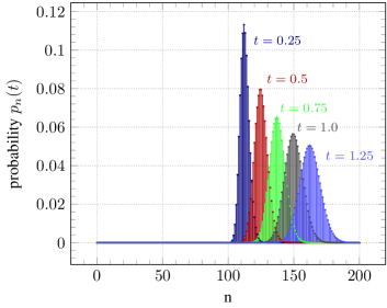
Refer to caption
(a) birth reaction 0Aβ=501A𝛽500𝐴1𝐴0A\xrightharpoonup{\;\beta=50\;}1A
Refer to caption
(b) pair creation reaction 0Aγ=252A𝛾250𝐴2𝐴0A\xrightharpoonup{\;\gamma=25\;}2A
Refer to caption
(c) decay reaction 1Aτ=40A𝜏41𝐴0𝐴1A\xrightharpoonup{\;\tau=4\;}0A
Refer to caption
(d) autocatalysis reaction 1Aα=122A𝛼121𝐴2𝐴1A\xrightharpoonup{\;\alpha=\tfrac{1}{2}\;}2A
Refer to caption
(e) pair annihilation reaction 2Aκ=1400A𝜅1402𝐴0𝐴2A\xrightharpoonup{\;\kappa=\tfrac{1}{40}\;}0A
Refer to caption
(f) catalytic decay reaction 2Aλ=1101A𝜆1102𝐴1𝐴2A\xrightharpoonup{\;\lambda=\tfrac{1}{10}\;}1A
Fig.  2: Discrete probability distributions for initial state |Ψ(0)=|100ketΨ0ket100\left|\Psi(0)\right\rangle=\left|100\right\rangle and for individual elementary reactions.

6.3 On compositionality of elementary non-binary reactions

Even though the results presented in Table 3 constitute a complete list of evolution formulae for individual non-binary chemical reactions, this does not yet provide a full answer to the question of which form the evolution of reaction systems composed of multiple non-binary chemical reactions would take. While the techniques of Theorem 7 remain applicable for such a generic non-binary reaction system, one would a priori have to compute the functions g(λ;x¯)𝑔𝜆¯𝑥g(\lambda;\underline{x}) and T¯(λ;x¯)¯𝑇𝜆¯𝑥\underline{T}(\lambda;\underline{x}) anew for each possible such reaction system. It would thus be desirable to find a technique that allows to simplify this computation via providing a form of composition law for solutions to chemical reaction systems assembled from elementary reactions. As a first step in this direction, we present a result for a reaction system composed of all four possible one-species non-binary elementary reactions:

Theorem 9.

Consider a 111-species reaction system with reactions

\displaystyle\emptyset 𝛽S,𝛾2Sformulae-sequence𝛽absent𝑆𝛾2𝑆\displaystyle\xrightharpoonup{\;\beta\;}S\,,\quad\emptyset\xrightharpoonup{\;\gamma\;}2S
S𝑆\displaystyle S 𝜏,S𝛼2S,formulae-sequence𝜏absent𝛼𝑆2𝑆\displaystyle\xrightharpoonup{\;\tau\;}\emptyset\,,\quad S\xrightharpoonup{\;\alpha\;}2S\,,

with parameters α,β,γ,τ0𝛼𝛽𝛾𝜏subscriptabsent0\alpha,\beta,\gamma,\tau\in\mathbb{R}_{\geq 0}. The reactions describe birth (B)𝐵(B), pair creation (C)𝐶(C), death (D)𝐷(D) and autocatalysis (A)𝐴(A) transitions. Then the probability generating function P(t;x)𝑃𝑡𝑥P(t;x), given P(0;x)𝑃0𝑥P(0;x), reads

P(t;x)𝑃𝑡𝑥\displaystyle P(t;x) =gBDA(t;x)gCDA(t;x)P(0;TDA(t;x)),absentsubscript𝑔𝐵𝐷𝐴𝑡𝑥subscript𝑔𝐶𝐷𝐴𝑡𝑥𝑃0subscript𝑇𝐷𝐴𝑡𝑥\displaystyle=g_{BDA}(t;x)g_{CDA}(t;x)P(0;T_{DA}(t;x))\,, (84)

where the concrete formulae differ slightly for the various possible choices of parameters. Let us for convenience introduce the notations (cf. Table 3)

TD(t;x)subscript𝑇𝐷𝑡𝑥\displaystyle T_{D}(t;x) :=Bern(etτ;x)assignabsent𝐵𝑒𝑟𝑛superscript𝑒𝑡𝜏𝑥\displaystyle:=Bern(e^{-t\tau};x) (85)
TA(t;x)subscript𝑇𝐴𝑡𝑥\displaystyle T_{A}(t;x) :=Geom(etα;x),assignabsent𝐺𝑒𝑜𝑚superscript𝑒𝑡𝛼𝑥\displaystyle:=Geom(e^{-t\alpha};x)\,,

and the following formulae for some standard probability generating functions (i.e. the alternative geometric, the Poisson and the 222-aerated Poisson distributions’ PGFs) [32, 33, 34]:

Geom2(p;x)𝐺𝑒𝑜subscript𝑚2𝑝𝑥\displaystyle Geom_{2}(p;x) :=p1x(1p)assignabsent𝑝1𝑥1𝑝\displaystyle:=\frac{p}{1-x(1-p)} (0<p1)0𝑝1\displaystyle(0<p\leq 1) (86)
Pois(p,x)𝑃𝑜𝑖𝑠𝑝𝑥\displaystyle Pois(p,x) :=ep(x1)assignabsentsuperscript𝑒𝑝𝑥1\displaystyle:=e^{p(x-1)}\quad (0p)0𝑝\displaystyle(0\leq p)
A2Pois(p,x)subscript𝐴2𝑃𝑜𝑖𝑠𝑝𝑥\displaystyle A_{2}Pois(p,x) :=ep(x21)assignabsentsuperscript𝑒𝑝superscript𝑥21\displaystyle:=e^{p(x^{2}-1)}\quad (0p).0𝑝\displaystyle(0\leq p)\,.

Case α=τ=0𝛼𝜏0\alpha=\tau=0:

TDAα=τ=0(t;x)superscriptsubscript𝑇𝐷𝐴𝛼𝜏0𝑡𝑥\displaystyle T_{DA}^{\alpha=\tau=0}(t;x) =xabsent𝑥\displaystyle=x (87)
gBDAα=τ=0(t;x)superscriptsubscript𝑔𝐵𝐷𝐴𝛼𝜏0𝑡𝑥\displaystyle g_{BDA}^{\alpha=\tau=0}(t;x) =Pois(βt;x)absent𝑃𝑜𝑖𝑠𝛽𝑡𝑥\displaystyle=Pois(\beta t;x)
gCDAα=τ=0(t;x)subscriptsuperscript𝑔𝛼𝜏0𝐶𝐷𝐴𝑡𝑥\displaystyle g^{\alpha=\tau=0}_{CDA}(t;x) =A2Pois(γt;x).absentsubscript𝐴2𝑃𝑜𝑖𝑠𝛾𝑡𝑥\displaystyle=A_{2}Pois(\gamma t;x)\,.

Case α=τ0𝛼𝜏0\alpha=\tau\neq 0:

TDAα=τ>0(t;x)superscriptsubscript𝑇𝐷𝐴𝛼𝜏0𝑡𝑥\displaystyle T_{DA}^{\alpha=\tau>0}(t;x) =TD(s(t);TA(s(t);x))absentsubscript𝑇𝐷𝑠𝑡subscript𝑇𝐴𝑠𝑡𝑥\displaystyle=T_{D}(s(t);T_{A}(s(t);x)) (88)
gBDAα=τ>0(t;x)superscriptsubscript𝑔𝐵𝐷𝐴𝛼𝜏0𝑡𝑥\displaystyle g_{BDA}^{\alpha=\tau>0}(t;x) =(Geom2(eαs(t);x))β/αabsentsuperscript𝐺𝑒𝑜subscript𝑚2superscript𝑒𝛼𝑠𝑡𝑥𝛽𝛼\displaystyle=\left(Geom_{2}\left(e^{-\alpha s(t)};x\right)\right)^{\beta/\alpha}
gCDAα=τ>0(t;x)superscriptsubscript𝑔𝐶𝐷𝐴𝛼𝜏0𝑡𝑥\displaystyle g_{CDA}^{\alpha=\tau>0}(t;x) =(Geom2(eαs(t);x))2γ/αabsentsuperscript𝐺𝑒𝑜subscript𝑚2superscript𝑒𝛼𝑠𝑡𝑥2𝛾𝛼\displaystyle=\left(Geom_{2}\left(e^{-\alpha s(t)};x\right)\right)^{2\gamma/\alpha}
eγt(x1)2Geom2(eαs(t);x)absentsuperscript𝑒𝛾𝑡superscript𝑥12𝐺𝑒𝑜subscript𝑚2superscript𝑒𝛼𝑠𝑡𝑥\displaystyle\qquad\cdot e^{\gamma t(x-1)^{2}Geom_{2}(e^{-\alpha s(t)};x)}
s(t)𝑠𝑡\displaystyle s(t) :=1αln(1+αt).assignabsent1𝛼1𝛼𝑡\displaystyle:=\frac{1}{\alpha}\ln(1+\alpha t)\,.

Case ατ𝛼𝜏\alpha\neq\tau and α>0,τ0formulae-sequence𝛼0𝜏0\alpha>0,\tau\geq 0:

TDAατ(t;x)superscriptsubscript𝑇𝐷𝐴𝛼𝜏𝑡𝑥\displaystyle T_{DA}^{\alpha\neq\tau}(t;x) =TD(sD(t);TA(sA(t);x))absentsubscript𝑇𝐷subscript𝑠𝐷𝑡subscript𝑇𝐴subscript𝑠𝐴𝑡𝑥\displaystyle=T_{D}(s_{D}(t);T_{A}(s_{A}(t);x)) (89)
gBDAατ(t;x)superscriptsubscript𝑔𝐵𝐷𝐴𝛼𝜏𝑡𝑥\displaystyle g_{BDA}^{\alpha\neq\tau}(t;x) =(Geom2(eαsA(t);x))β/αabsentsuperscript𝐺𝑒𝑜subscript𝑚2superscript𝑒𝛼subscript𝑠𝐴𝑡𝑥𝛽𝛼\displaystyle=\left(Geom_{2}\left(e^{-\alpha s_{A}(t)};x\right)\right)^{\beta/\alpha}
gCDAατ(t;x)superscriptsubscript𝑔𝐶𝐷𝐴𝛼𝜏𝑡𝑥\displaystyle g_{CDA}^{\alpha\neq\tau}(t;x) =(Geom2(eαsA(t);x))γ(α+τ)/α2absentsuperscript𝐺𝑒𝑜subscript𝑚2superscript𝑒𝛼subscript𝑠𝐴𝑡𝑥𝛾𝛼𝜏superscript𝛼2\displaystyle=\left(Geom_{2}\left(e^{-\alpha s_{A}(t)};x\right)\right)^{\gamma(\alpha+\tau)/\alpha^{2}}
efCDA(t;x)Geom2(eαsA(t);x)absentsuperscript𝑒subscript𝑓𝐶𝐷𝐴𝑡𝑥𝐺𝑒𝑜subscript𝑚2superscript𝑒𝛼subscript𝑠𝐴𝑡𝑥\displaystyle\qquad\cdot e^{f_{CDA}(t;x)Geom_{2}(e^{-\alpha s_{A}(t)};x)}
fCDA(t;x)subscript𝑓𝐶𝐷𝐴𝑡𝑥\displaystyle f_{CDA}(t;x) =γα+τ((x1)2(et(ατ)1)\displaystyle=\frac{\gamma}{\alpha+\tau}\bigg{(}(x-1)^{2}\left(e^{t(\alpha-\tau)}-1\right)
+(x1)(1+τα)(1et(ατ)))\displaystyle\qquad+(x-1)(1+\tfrac{\tau}{\alpha})\left(1-e^{t(\alpha-\tau)}\right)\bigg{)}
τsD(t)𝜏subscript𝑠𝐷𝑡\displaystyle\tau s_{D}(t) :=ln(ατe(τα)tατ)assignabsent𝛼𝜏superscript𝑒𝜏𝛼𝑡𝛼𝜏\displaystyle:=\ln\left(\frac{\alpha-\tau e^{(\tau-\alpha)t}}{\alpha-\tau}\right)
αsA(t)𝛼subscript𝑠𝐴𝑡\displaystyle\alpha s_{A}(t) :=ln(αe(ατ)tτατ).assignabsent𝛼superscript𝑒𝛼𝜏𝑡𝜏𝛼𝜏\displaystyle:=\ln\left(\frac{\alpha e^{(\alpha-\tau)t}-\tau}{\alpha-\tau}\right)\,.

Case α=0𝛼0\alpha=0 and τ>0𝜏0\tau>0:

TDAα=0,τ>0(t;x)superscriptsubscript𝑇𝐷𝐴formulae-sequence𝛼0𝜏0𝑡𝑥\displaystyle T_{DA}^{\alpha=0,\tau>0}(t;x) =TD(t;x)absentsubscript𝑇𝐷𝑡𝑥\displaystyle=T_{D}(t;x) (90)
gBDAα=0,τ>0(t;x)superscriptsubscript𝑔𝐵𝐷𝐴formulae-sequence𝛼0𝜏0𝑡𝑥\displaystyle g_{BDA}^{\alpha=0,\tau>0}(t;x) =Pois(βτ(1etτ);x)absent𝑃𝑜𝑖𝑠𝛽𝜏1superscript𝑒𝑡𝜏𝑥\displaystyle=Pois(\tfrac{\beta}{\tau}\left(1-e^{-t\tau});x\right)
gCDAα=0,τ>0(t;x)superscriptsubscript𝑔𝐶𝐷𝐴formulae-sequence𝛼0𝜏0𝑡𝑥\displaystyle g_{CDA}^{\alpha=0,\tau>0}(t;x) =Pois(γτ(1etτ)2;x)\displaystyle=Pois(\tfrac{\gamma}{\tau}\left(1-e^{-t\tau})^{2};x\right)\cdot
A2Pois(γ2τ(1e2tτ);x).absentsubscript𝐴2𝑃𝑜𝑖𝑠𝛾2𝜏1superscript𝑒2𝑡𝜏𝑥\displaystyle\;\cdot A_{2}Pois(\tfrac{\gamma}{2\tau}\left(1-e^{-2t\tau});x\right)\,.
Proof.

Via applying Theorem 7, one obtains formulae for P(t;x)𝑃𝑡𝑥P(t;x) in the various cases of interest that may then be brought into the forms as presented by an elementary, if somewhat tedious “factorization” of the formulae into compounds and convolutions of probability generating functions. See Appendix D for further details. ∎

It might be worthwhile to consider the following auxiliary formula, which expresses the fact that taking a power of the Geom2(p;x)𝐺𝑒𝑜subscript𝑚2𝑝𝑥Geom_{2}(p;x) PGF with a positive real exponent μ𝜇\mu results in a well-posed PGF*†*†*†For the case 0<μ<10𝜇10<\mu<1, we find (k+μ1k)=Γ(μ+k)k!Γ(μ)=1k!(μ)(k),binomial𝑘𝜇1𝑘Γ𝜇𝑘𝑘Γ𝜇1𝑘superscript𝜇𝑘\binom{k+\mu-1}{k}=\frac{\Gamma(\mu+k)}{k!\Gamma(\mu)}=\frac{1}{k!}(\mu)^{(k)}\,, with (x)(k)superscript𝑥𝑘(x)^{(k)} the rising factorial, i.e. (x)(0)=1superscript𝑥01(x)^{(0)}=1 and x(k)=x(x+1)(x+k1)superscript𝑥𝑘𝑥𝑥1𝑥𝑘1x^{(k)}=x(x+1)\dotsc(x+k-1) for k>0𝑘0k>0.:

(Geom2(p;x))μ=(p1x(1p))μsuperscript𝐺𝑒𝑜subscript𝑚2𝑝𝑥𝜇superscript𝑝1𝑥1𝑝𝜇\displaystyle\left(Geom_{2}(p;x)\right)^{\mu}=\left(\frac{p}{1-x(1-p)}\right)^{\mu} (91)
=δμ,0+δμ>0pμn0(n+μ1n)(1p)nxn.absentsubscript𝛿𝜇0subscript𝛿𝜇0superscript𝑝𝜇subscript𝑛0binomial𝑛𝜇1𝑛superscript1𝑝𝑛superscript𝑥𝑛\displaystyle\quad=\delta_{\mu,0}+\delta_{\mu>0}p^{\mu}\sum_{n\geq 0}\binom{n+\mu-1}{n}(1-p)^{n}x^{n}\,.

For the permissible paramter range of the Geom2(p;x)𝐺𝑒𝑜subscript𝑚2𝑝𝑥Geom_{2}(p;x) (0<p10𝑝10<p\leq 1), we thus observe that all coefficients of xnsuperscript𝑥𝑛x^{n} for all n0𝑛0n\geq 0 are non-negative real numbers, and evidently Geom2(p;1)μ=1𝐺𝑒𝑜subscript𝑚2superscript𝑝1𝜇1Geom_{2}(p;1)^{\mu}=1.

Since admittedly the results of Theorem 9 are somewhat hard to interpret from the presentation in terms of generating functions, we exhibit in Figure 3 a set of illustrative examples of parameter choices and their respective effects on the first three cumulants and on the probability distributions. Moreover, in Figure 4 we provide ternary data plots for the effects of relative parameter choices for reaction systems of three of the four possible semi-linear reactions for illustration.

A particularly interesting effect concerns the example of the reaction system

1Aα=1/32A,0Aγ=1/32A,1Aτ=1/30A,formulae-sequence𝛼131𝐴2𝐴formulae-sequence𝛾130𝐴2𝐴𝜏131𝐴0𝐴1A\xrightharpoonup{\;\alpha=1/3\;}2A\,,\quad 0A\xrightharpoonup{\;\gamma=1/3\;}2A\,,\quad 1A\xrightharpoonup{\;\tau=1/3\;}0A\,, (92)

for which we depict the evolution of the first three cumulants in Figure 3a as well as the evolution of the probability distribution in Figure 3b. Notably, the mean (i.e. the first cumulant) remains fixed at the initial value (in this case c1(0)=100subscript𝑐10100c_{1}(0)=100), and throughout the evolution the probability distribution effectively undergoes a progressive broadening of the distribution around this mean value.

In Figures 3c and 3d, we depict cumulant and probability distribution evolutions for a variant of a birth-death system, namely a system with also a pair creation reaction,

0Aβ=1/51A,0Aγ=3/52A,1Aτ=1/50A.formulae-sequence𝛽150𝐴1𝐴formulae-sequence𝛾350𝐴2𝐴𝜏151𝐴0𝐴0A\xrightharpoonup{\;\beta=1/5\;}1A\,,\quad 0A\xrightharpoonup{\;\gamma=3/5\;}2A\,,\quad 1A\xrightharpoonup{\;\tau=1/5\;}0A\,. (93)

It is instructive to consider the exact formula for the probability generating function of this system (cf. (90)), which for an initial state |Ψ(0)=|MketΨ0ket𝑀\left|\Psi(0)\right\rangle=\left|M\right\rangle of precisely M𝑀M particles (i.e. for P(0;x)=xM𝑃0𝑥superscript𝑥𝑀P(0;x)=x^{M}) reads

P(t;x)𝑃𝑡𝑥\displaystyle P(t;x) =eγ2τ(1e2tτ)(x21)absentsuperscript𝑒𝛾2𝜏1superscript𝑒2𝑡𝜏superscript𝑥21\displaystyle=e^{\tfrac{\gamma}{2\tau}\left(1-e^{-2t\tau}\right)(x^{2}-1)} (94)
e[γτ(1etτ)2+βτ(1etτ)](x1)absentsuperscript𝑒delimited-[]𝛾𝜏superscript1superscript𝑒𝑡𝜏2𝛽𝜏1superscript𝑒𝑡𝜏𝑥1\displaystyle\quad\cdot e^{\left[\tfrac{\gamma}{\tau}\left(1-e^{-t\tau}\right)^{2}+\tfrac{\beta}{\tau}\left(1-e^{-t\tau}\right)\right](x-1)}
(Bern(etτ;x))M.absentsuperscript𝐵𝑒𝑟𝑛superscript𝑒𝑡𝜏𝑥𝑀\displaystyle\qquad\cdot(Bern(e^{-t\tau};x))^{M}\,.

Taking the limit t𝑡t\to\infty and noting that

limtBern(etτ;x)=1,subscript𝑡𝐵𝑒𝑟𝑛superscript𝑒𝑡𝜏𝑥1\lim\limits_{t\to\infty}Bern(e^{-t\tau};x)=1\,,

we find the limit distribution

limtP(t;x)=eγ2τ(x21)+β+γτ(x1).subscript𝑡𝑃𝑡𝑥superscript𝑒𝛾2𝜏superscript𝑥21𝛽𝛾𝜏𝑥1\lim\limits_{t\to\infty}P(t;x)=e^{\tfrac{\gamma}{2\tau}(x^{2}-1)+\tfrac{\beta+\gamma}{\tau}(x-1)}\,. (95)

We present in Figure 4 a number of ternary data plots the evolution of first and second cumulants for this reaction system for illustration.

As a final example, we depict in Figures 3e and 3f the evolution of a reaction system with all four types of non-binary one-species reactions. Depending on the choices of the four reaction rates involved, we find that the system evolves in a fashion either similar to the reaction system (92) or to the reaction system (93). A representative example for a choice of parameters that leads to dynamical behaviour akin to that of the reaction system (93) is depicted in Figures 3e and 3f.

To conclude our treatment of non-binary chemical reaction systems, it is worthwhile noting that there exists previous work in the mathematical chemistry literature [11] on closed-form exact solutions for probability generating functions of multi-species non-binary reactions except for the autocatalytic reaction types. Since our formulae cover an arbitrary single-species non-binary reaction system, it appears worthwhile to consider the generalization of our Theorem 9 to the multi-species cases. We plan to present such results in future work.
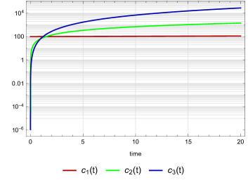
Refer to caption
(a) 1Aα=1/32A𝛼131𝐴2𝐴1A\xrightharpoonup{\;\alpha=1/3\;}2A, 0Aγ=1/32A𝛾130𝐴2𝐴0A\xrightharpoonup{\;\gamma=1/3\;}2A, 1Aτ=1/30A𝜏131𝐴0𝐴1A\xrightharpoonup{\;\tau=1/3\;}0A
Refer to caption
(b) distributions |Ψ(t)ketΨ𝑡\left|\Psi(t)\right\rangle for a)
Refer to caption
(c) 0Aβ=0.21A𝛽0.20𝐴1𝐴0A\xrightharpoonup{\;\beta=0.2\;}1A, 0Aγ=0.62A𝛾0.60𝐴2𝐴0A\xrightharpoonup{\;\gamma=0.6\;}2A, 1Aτ=0.20A𝜏0.21𝐴0𝐴1A\xrightharpoonup{\;\tau=0.2\;}0A
Refer to caption
(d) distributions |Ψ(t)ketΨ𝑡\left|\Psi(t)\right\rangle for c)
Refer to caption
(e) 0A0.41A0.40𝐴1𝐴0A\xrightharpoonup{0.4\;}1A, 0A0.22A0.20𝐴2𝐴0A\xrightharpoonup{0.2\;}2A, 1A0.30A0.31𝐴0𝐴1A\xrightharpoonup{0.3\;}0A, 1A0.12A0.11𝐴2𝐴1A\xrightharpoonup{0.1\;}2A
Refer to caption
(f) distributions |Ψ(t)ketΨ𝑡\left|\Psi(t)\right\rangle for e)
Fig.  3: First three cumulants ci(t)subscript𝑐𝑖𝑡c_{i}(t) (i=1,2,3𝑖123i=1,2,3) and discrete probability distributions |Ψ(t)=n0pn(t)|nketΨ𝑡subscript𝑛0subscript𝑝𝑛𝑡ket𝑛\left|\Psi(t)\right\rangle=\sum_{n\geq 0}p_{n}(t)\left|n\right\rangle for systems of non-binary reactions with initial state |Ψ(0)=|100ketΨ0ket100\left|\Psi(0)\right\rangle=\left|100\right\rangle.
Refer to caption
(a) Mean number of particles at time t=1𝑡1t=1
Refer to caption
(b) Variance of number of particles at time t=1𝑡1t=1
Refer to caption
(c) Mean number of particles at time t=4𝑡4t=4
Refer to caption
(d) Variance of number of particles at time t=4𝑡4t=4
Refer to caption
(e) Mean number of particles at time t=16𝑡16t=16
Refer to caption
(f) Variance of number of particles at time t=16𝑡16t=16
Fig.  4: Ternary parameter dependence plot (β+γ+τ=1𝛽𝛾𝜏1\beta+\gamma+\tau=1) of the first and second cumulants (mean c1(t)subscript𝑐1𝑡c_{1}(t) and variance c2(t)subscript𝑐2𝑡c_{2}(t)) for a reaction system composed of birth, pair creation and decay reactions, with initial state |Ψ(0)=|100ketΨ0ket100\left|\Psi(0)\right\rangle=\left|100\right\rangle. In a)a), c)c) and e)e), we observe that with increasing decay rate τ𝜏\tau the mean particle number decreases over time, while the relative strengths of β𝛽\beta and γ𝛾\gamma have little influence on the dynamics. In contrast, the time evolution of the variance as depicted in b)b), d)d) and f)f) is more sensitive to the ratio of β𝛽\beta and γ𝛾\gamma, as are all higher cumulants (not presented).

6.4 Closed-form solutions for probability generating functions of single-species binary reactions

In the 1960’s, McQuarrie [12, 2] suggested to solve the problem of finding the probability generating functions for single-species binary chemical reaction systems and for a deterministic initial state |Ψ(0)=|MketΨ0ket𝑀\left|\Psi(0)\right\rangle=\left|M\right\rangle, whence for P(0;x)=xM𝑃0𝑥superscript𝑥𝑀P(0;x)=x^{M}, via a separation of variables Ansatz of the form

P(t;x)=n0AM;nTn(t)Xn(x).𝑃𝑡𝑥subscript𝑛0subscript𝐴𝑀𝑛subscript𝑇𝑛𝑡subscript𝑋𝑛𝑥P(t;x)=\sum_{n\geq 0}A_{M;n}T_{n}(t)X_{n}(x)\,. (96)

Here, the functions Xn(x)subscript𝑋𝑛𝑥X_{n}(x) are polynomials, with degree(Xn)=n𝑑𝑒𝑔𝑟𝑒𝑒subscript𝑋𝑛𝑛degree(X_{n})=n. The time-dependent functions Tn(t)subscript𝑇𝑛𝑡T_{n}(t) read

Tn(t)=eλnt,subscript𝑇𝑛𝑡superscript𝑒subscript𝜆𝑛𝑡T_{n}(t)=e^{\lambda_{n}t}\,, (97)

while the constant coefficients AM;nsubscript𝐴𝑀𝑛A_{M;n}\in\mathbb{R} are determined by the initial condition P(0;x)=xM𝑃0𝑥superscript𝑥𝑀P(0;x)=x^{M},

xM=n0AM;nXn(x)=n=0MAM;nXn(x).superscript𝑥𝑀subscript𝑛0subscript𝐴𝑀𝑛subscript𝑋𝑛𝑥superscriptsubscript𝑛0𝑀subscript𝐴𝑀𝑛subscript𝑋𝑛𝑥x^{M}=\sum_{n\geq 0}A_{M;n}X_{n}(x)=\sum_{n=0}^{M}A_{M;n}X_{n}(x)\,. (98)

In order for McQuarrie’s Ansatz to be consistent, it is thus strictly necessary that the polynomials Xn(x)subscript𝑋𝑛𝑥X_{n}(x) form a complete system of eigenfunctions of the Hamiltonian (x^,x)^𝑥subscript𝑥\mathcal{H}\equiv\mathcal{H}(\hat{x},\partial_{x}) in the Bargmann-Fock basis (compare (56) for the one-species case upon invoking the one-to-one correspondence described in (27)):

Xn(x)=λnXn(x).subscript𝑋𝑛𝑥subscript𝜆𝑛subscript𝑋𝑛𝑥\mathcal{H}X_{n}(x)=\lambda_{n}X_{n}(x)\,. (99)

In other words, it must be the case that precisely one degree n𝑛n polynomial Xn(x)subscript𝑋𝑛𝑥X_{n}(x) is available for each non-negative integer value n𝑛n.

McQuarrie suggests the following approach: the functions Xn(x)subscript𝑋𝑛𝑥X_{n}(x) should be found as certain orthogonal polynomials of the Jacobi type. Let us briefly review some of the necessary background material on this mathematical structure.

6.5 Classical Jacobi polynomials and orthogonality

The Jacobi-type second-order differential operator*‡*‡*‡In this section, for notational coherence with the cited standard reference we temporarily denote the variables by z𝑧z and drop the notation z^^𝑧\hat{z} in favor of just z𝑧z for the linear operator of multiplication by z𝑧z. (cf. the standard reference book [34], chapter 18, p. 445, Table 18.8.1)

DJacα,βsubscriptsuperscript𝐷𝛼𝛽𝐽𝑎𝑐\displaystyle D^{\alpha,\beta}_{Jac} :=(1z2)2z2+q(α,β)(z)zassignabsent1superscript𝑧2superscript2superscript𝑧2superscript𝑞𝛼𝛽𝑧𝑧\displaystyle:=(1-z^{2})\tfrac{\partial^{2}}{\partial z^{2}}+q^{(\alpha,\beta)}(z)\tfrac{\partial}{\partial z} (100)
q(α,β)(z)superscript𝑞𝛼𝛽𝑧\displaystyle q^{(\alpha,\beta)}(z) =(βα(α+β+2)z)absent𝛽𝛼𝛼𝛽2𝑧\displaystyle=(\beta-\alpha-(\alpha+\beta+2)z)

with real parameters

α,β>1𝛼𝛽1\alpha,\beta>-1 (101)

is known to possess a system of orthogonal polynomials {Pn(α,β)(z)}n0subscriptsubscriptsuperscript𝑃𝛼𝛽𝑛𝑧𝑛0\{P^{(\alpha,\beta)}_{n}(z)\}_{n\geq 0}, the so-called classical Jacobi polynomials, as its complete basis of eigenfunctions. More explicitly (cf. e.g. [34], Equation 18.5.8),

Pn(α,β)(z)subscriptsuperscript𝑃𝛼𝛽𝑛𝑧\displaystyle P^{(\alpha,\beta)}_{n}(z) (102)
=2n=0n(n+α)(n+βn)(z1)n(z+1),absentsuperscript2𝑛superscriptsubscript0𝑛binomial𝑛𝛼binomial𝑛𝛽𝑛superscript𝑧1𝑛superscript𝑧1\displaystyle\quad=2^{-n}\sum_{\ell=0}^{n}\binom{n+\alpha}{\ell}\binom{n+\beta}{n-\ell}(z-1)^{n-\ell}(z+1)^{\ell}\,,

satisfying the eigenequation

DJacα,βPn(α,β)(z)=n(n+α+β+1)Pn(α,β)(z).subscriptsuperscript𝐷𝛼𝛽𝐽𝑎𝑐superscriptsubscript𝑃𝑛𝛼𝛽𝑧𝑛𝑛𝛼𝛽1superscriptsubscript𝑃𝑛𝛼𝛽𝑧D^{\alpha,\beta}_{Jac}P_{n}^{(\alpha,\beta)}(z)=-n(n+\alpha+\beta+1)P_{n}^{(\alpha,\beta)}(z)\,. (103)

The orthogonality property is found by defining for each admissible choice of parameters α,β>1𝛼𝛽1\alpha,\beta>-1 an inner product Φα,βsubscriptΦ𝛼𝛽\Phi_{\alpha,\beta} on the space of polynomials,

Φα,β(p(z),q(z))subscriptΦ𝛼𝛽𝑝𝑧𝑞𝑧\displaystyle\Phi_{\alpha,\beta}(p(z),q(z)) :=1+1𝑑zwα,β(z)p(z)q(z)assignabsentsuperscriptsubscript11differential-d𝑧subscript𝑤𝛼𝛽𝑧𝑝𝑧𝑞𝑧\displaystyle:=\int_{-1}^{+1}dz\;w_{\alpha,\beta}(z)p(z)q(z) (104)
wα,β(z)subscript𝑤𝛼𝛽𝑧\displaystyle w_{\alpha,\beta}(z) :=(1z)α(1+z)β.assignabsentsuperscript1𝑧𝛼superscript1𝑧𝛽\displaystyle:=(1-z)^{\alpha}(1+z)^{\beta}\,.

It is one of the classical results of the theory of orthogonal polynomials that for all n0𝑛0n\geq 0

Pn(α,β)(z)Lα,β2([1,1]).superscriptsubscript𝑃𝑛𝛼𝛽𝑧subscriptsuperscript𝐿2𝛼𝛽11P_{n}^{(\alpha,\beta)}(z)\in L^{2}_{\alpha,\beta}([-1,1])\,. (105)

Here, Lα,β2([1,1])subscriptsuperscript𝐿2𝛼𝛽11L^{2}_{\alpha,\beta}([-1,1]) denotes the space of functions on the interval [1,1]11[-1,1] which are square-integrable w.r.t. the integral against the weight function wα,β(z)subscript𝑤𝛼𝛽𝑧w_{\alpha,\beta}(z). Moreover, orthogonality manifests itself as

Φα,β(Pm(α,β)(z),Pn(α,β)(z))=δm,nϕα,β(n),subscriptΦ𝛼𝛽superscriptsubscript𝑃𝑚𝛼𝛽𝑧superscriptsubscript𝑃𝑛𝛼𝛽𝑧subscript𝛿𝑚𝑛subscriptitalic-ϕ𝛼𝛽𝑛\Phi_{\alpha,\beta}\left(P_{m}^{(\alpha,\beta)}(z),P_{n}^{(\alpha,\beta)}(z)\right)=\delta_{m,n}\phi_{\alpha,\beta}(n)\,, (106)

with ϕα,β(n)>0subscriptitalic-ϕ𝛼𝛽𝑛subscriptabsent0\phi_{\alpha,\beta}(n)\in\mathbb{R}_{>0} some non-zero real numbers.

6.6 The case of binary reactions and a technical problem

As we shall see momentarily, the type of differential operators we are interested in when studying chemical reaction systems, while superficially of the structure of the Jacobi-type differential operators, is precisely not fulfilling the parameter constraint (101). The problem presents itself as follows:

Lemma 2.

Consider a chemical reaction system of one species of particles and the reactions

Ard,2Ark,2ArA,formulae-sequencesubscript𝑟𝑑𝐴formulae-sequencesubscript𝑟𝑘2𝐴subscript𝑟2𝐴𝐴\displaystyle A\xrightharpoonup{\;r_{d}\;}\emptyset\,,\quad 2\>A\xrightharpoonup{\;r_{k}\;}\emptyset\,,\quad 2\>A\xrightharpoonup{\;r_{\ell}\;}A\,, (107)

where rk+r>0subscript𝑟𝑘subscript𝑟0r_{k}+r_{\ell}>0 (i.e. the system involves at least one binary reaction), and where we assume for simplicity and without loss of generalityNote that generic values of rksubscript𝑟𝑘r_{k} and rsubscript𝑟r_{\ell} may be achieved via appropriately rescaling t𝑡t. See Proposition 6 for the precise details.

rk+r=1.subscript𝑟𝑘subscript𝑟1r_{k}+r_{\ell}=1\,.

The corresponding Hamiltonian reads in the Bargmann-Fock basis

\displaystyle\mathcal{H} =rd(1x^)xabsentsubscript𝑟𝑑1^𝑥𝑥\displaystyle=r_{d}(1-\hat{x})\tfrac{\partial}{\partial x} (108)
rk(1x^2)(x)2+r(x^x^2)(x)2.subscript𝑟𝑘1superscript^𝑥2superscript𝑥2subscript𝑟^𝑥superscript^𝑥2superscript𝑥2\displaystyle\quad r_{k}(1-\hat{x}^{2})\left(\tfrac{\partial}{\partial x}\right)^{2}+r_{\ell}(\hat{x}-\hat{x}^{2})\left(\tfrac{\partial}{\partial x}\right)^{2}\,.

Then one can bring the Jacobi-type differential operator DJacα,βsuperscriptsubscript𝐷𝐽𝑎𝑐𝛼𝛽D_{Jac}^{\alpha,\beta} as presented in (100) via the affine transformation

x(z)=r2+(1r2)z𝑥𝑧subscript𝑟21subscript𝑟2𝑧x(z)=\frac{r_{\ell}}{2}+\left(1-\frac{r_{\ell}}{2}\right)z (109)

into the form of \mathcal{H}, which entails that

(+n(n+rd1))Pn(1;rd1)(xr21r2)=0.𝑛𝑛subscript𝑟𝑑1subscriptsuperscript𝑃1subscript𝑟𝑑1𝑛𝑥subscript𝑟21subscript𝑟20\left(\mathcal{H}+n(n+r_{d}-1)\right)P^{(-1;r_{d}-1)}_{n}\left(\frac{x-\frac{r_{\ell}}{2}}{1-\frac{r_{\ell}}{2}}\right)=0\,. (110)

Unfortunately, we thus encounter for all of the interesting reaction rate choices yielding binary chemical reaction systems the “illegal” parameter ranges, since we are interested specifically in the cases

(i) α=1,β=rd1>1formulae-sequence𝛼1𝛽subscript𝑟𝑑11\displaystyle\alpha=-1,\;\beta=r_{d}-1>-1 (111)
(ii) α=1,β=1(i.e. rd=0).formulae-sequence𝛼1𝛽1i.e. subscript𝑟𝑑0\displaystyle\alpha=-1,\;\beta=-1\quad(\text{i.e.\ }r_{d}=0)\,.

We encounter the following technical problems for these two types of parameter choices:

  • (i)𝑖(i)

    Case α=1,β>1formulae-sequence𝛼1𝛽1\alpha=-1,\beta>-1: With respect to the inner product Φ1,βsubscriptΦ1𝛽\Phi_{-1,\beta} as defined in (104) (with the variable named x𝑥x from hereon), we find that the degree zero polynomial

    P0(1,β)(x)=1subscriptsuperscript𝑃1𝛽0𝑥1P^{(-1,\beta)}_{0}(x)=1

    is not square-integrable,

    P0(1,β)(x)L1,β2([1,1]).subscriptsuperscript𝑃1𝛽0𝑥subscriptsuperscript𝐿21𝛽11P^{(-1,\beta)}_{0}(x)\not\in L^{2}_{-1,\beta}([-1,1])\,.

    Therefore, the set {Pn(1,β)(x)}n0subscriptsubscriptsuperscript𝑃1𝛽𝑛𝑥𝑛0\{P^{(-1,\beta)}_{n}(x)\}_{n\geq 0} fails to constitute a complete set of eigenfunctions of the operator \mathcal{H}.

  • (ii)𝑖𝑖(ii)

    Case α=1,β=1formulae-sequence𝛼1𝛽1\alpha=-1,\beta=-1: In addition to the failure of P0(1,1)(x)subscriptsuperscript𝑃110𝑥P^{(-1,-1)}_{0}(x) to be square-integrable w.r.t. the inner product Φ1,1subscriptΦ11\Phi_{-1,-1}, we moreover find from the explicit formula (LABEL:eq:JacExpl) for the Jacobi polynomials that

    P1(1,1)(x)=0.subscriptsuperscript𝑃111𝑥0P^{(-1,-1)}_{1}(x)=0\,. (112)

    In other words, in this case we lack the degree zero and the degree one eigenfunctions, and thus again do not obtain a complete system of eigenfunctions.

As it stands, one would thus have to conclude that McQuarrie’s approach to binary chemical reaction systems is ill-conceived.

A resolution of the problem of incompleteness of the eigenbasis has been provided by Kwon and Littlejohn [13, 15, 14, 16] (see also their survey article [35]). They observe first that any constant function and any linear function are solutions to the Jacobi type differential equation, and that moreover the family {Pn(α,β)(x)}n2subscriptsubscriptsuperscript𝑃𝛼𝛽𝑛𝑥𝑛2\{P^{(\alpha,\beta)}_{n}(x)\}_{n\geq 2} even at the problematic parameter values α=1𝛼1\alpha=-1 and β1𝛽1\beta\geq-1 remains an orthogonal family of eigenfunctions. Their key insight is then to consider an alternative notion of orthogonality, so-called Sobolev-orthogonality, which admits to construct a family {P~n(α,β)}n0subscriptsubscriptsuperscript~𝑃𝛼𝛽𝑛𝑛0\{\tilde{P}^{(\alpha,\beta)}_{n}\}_{n\geq 0} that is a complete system of eigenfunctions and orthogonal w.r.t. a Sobolev-type inner product.

We quote from [16] the relevant material (cf. Propositions 4.2 and 4.3 of loc cit):

Proposition 3.

Let the Sobolev inner products ΦA,B(1,1)subscriptsuperscriptΦ11𝐴𝐵\Phi^{(-1,-1)}_{A,B} and ΦC(1,β)superscriptsubscriptΦ𝐶1𝛽\Phi_{C}^{(-1,\beta)} (for β>1𝛽1\beta>-1) be defined as follows (for p,q[x]𝑝𝑞delimited-[]𝑥p,q\in\mathbb{R}[x] some polynomials with real coefficients)

ΦA,B(1,1)(p,q)subscriptsuperscriptΦ11𝐴𝐵𝑝𝑞\displaystyle\Phi^{(-1,-1)}_{A,B}(p,q) :=Ap(1)q(1)+Bp(1)q(1)assignabsent𝐴𝑝1𝑞1𝐵𝑝1𝑞1\displaystyle:=Ap(1)q(1)+Bp(-1)q(-1) (113)
+1+1𝑑xp(x)q(x)superscriptsubscript11differential-d𝑥superscript𝑝𝑥superscript𝑞𝑥\displaystyle\quad+\int_{-1}^{+1}dx\;p^{\prime}(x)q^{\prime}(x)
ΦC(1,β)(p,q)subscriptsuperscriptΦ1𝛽𝐶𝑝𝑞\displaystyle\Phi^{(-1,\beta)}_{C}(p,q) :=Cp(1)q(1)(β>1)assignabsent𝐶𝑝1𝑞1𝛽1\displaystyle:=Cp(1)q(1)\quad\qquad(\beta>-1)
+1+1𝑑x(x+1)β+1p(x)q(x).superscriptsubscript11differential-d𝑥superscript𝑥1𝛽1superscript𝑝𝑥superscript𝑞𝑥\displaystyle\quad+\int_{-1}^{+1}dx\;(x+1)^{\beta+1}p^{\prime}(x)q^{\prime}(x)\,.

Here, p(x)superscript𝑝𝑥p^{\prime}(x) and q(x)superscript𝑞𝑥q^{\prime}(x) denote the first derivatives of the polynomials, and A,B,C𝐴𝐵𝐶A,B,C\in\mathbb{R} are some parameters, which have to satisfy the following conditions: for ΦA,B(1,1)subscriptsuperscriptΦ11𝐴𝐵\Phi^{(-1,-1)}_{A,B}, A𝐴A and B𝐵B must verify

A+B>0,A(γ+1)2+B(γ1)2+20formulae-sequence𝐴𝐵0𝐴superscript𝛾12𝐵superscript𝛾1220\displaystyle A+B>0\,,\quad A(\gamma+1)^{2}+B(\gamma-1)^{2}+2\neq 0 (114)
A(γ+1)+B(γ1)=0𝐴𝛾1𝐵𝛾10\displaystyle\quad A(\gamma+1)+B(\gamma-1)=0
γ:=(BA)/(A+B),assign𝛾𝐵𝐴𝐴𝐵\displaystyle\quad\gamma:=(B-A)/(A+B)\,,

while for ΦC(1,β)superscriptsubscriptΦ𝐶1𝛽\Phi_{C}^{(-1,\beta)} the parameter C𝐶C must verify

C>0.𝐶0C>0\,. (115)

Then the Sobolev-Jacobi orthogonal polynomials P~n(α,β)(x)subscriptsuperscript~𝑃𝛼𝛽𝑛𝑥\tilde{P}^{(\alpha,\beta)}_{n}(x) are defined for α=1,β=1formulae-sequence𝛼1𝛽1\alpha=-1,\beta=-1 as

P~0(1,1)(x):=1assignsubscriptsuperscript~𝑃110𝑥1\displaystyle\tilde{P}^{(-1,-1)}_{0}(x):=1 (116)
P~1(1,1)(x):=x+γassignsubscriptsuperscript~𝑃111𝑥𝑥𝛾\displaystyle\tilde{P}^{(-1,-1)}_{1}(x):=x+\gamma
P~n2(1,1)(x):=(2n2n)1\displaystyle\tilde{P}^{(-1,-1)}_{n\geq 2}(x):=\binom{2n-2}{n}^{-1}\cdot
k=1n1(n1k)(n1nk)(x1)nk(x+1)k,\displaystyle\;\cdot\sum_{k=1}^{n-1}\binom{n-1}{k}\binom{n-1}{n-k}(x-1)^{n-k}(x+1)^{k}\,,

where γ=(BA)/(A+B)𝛾𝐵𝐴𝐴𝐵\gamma=(B-A)/(A+B), while for the parameters α=1,β>1formulae-sequence𝛼1𝛽1\alpha=-1,\beta>-1 one defines

P~0(1,β)(x):=1assignsuperscriptsubscript~𝑃01𝛽𝑥1\displaystyle\tilde{P}_{0}^{(-1,\beta)}(x):=1 (117)
P~1(1,β)(x):=x1assignsuperscriptsubscript~𝑃11𝛽𝑥𝑥1\displaystyle\tilde{P}_{1}^{(-1,\beta)}(x):=x-1
P~n2(1,β)(x):=(2n+β1n)1assignsuperscriptsubscript~𝑃𝑛21𝛽𝑥superscriptbinomial2𝑛𝛽1𝑛1\displaystyle\tilde{P}_{n\geq 2}^{(-1,\beta)}(x):=\binom{2n+\beta-1}{n}^{-1}
k=0n(n1k)(n+βnk)(x1)nk(x+1)k.\displaystyle\;\cdot\sum_{k=0}^{n}\binom{n-1}{k}\binom{n+\beta}{n-k}(x-1)^{n-k}(x+1)^{k}\,.

Then the P~n(α,β)(x)subscriptsuperscript~𝑃𝛼𝛽𝑛𝑥\tilde{P}^{(\alpha,\beta)}_{n}(x) form a complete orthogonal system of polynomial eigenfunctions of the Jacobi differential operator at parameters in the aforementioned parameter ranges.

The readers may have noticed that indeed the Sobolev-Jacobi polynomials P~n(α,β)(x)subscriptsuperscript~𝑃𝛼𝛽𝑛𝑥\tilde{P}^{(\alpha,\beta)}_{n}(x) as defined above coincide for n2𝑛2n\geq 2 with the monic versions of the classical Jacobi polynomials (i.e. a different normalization choice where in each polynomial of degree n𝑛n the coefficient of xnsuperscript𝑥𝑛x^{n} is normalized to be 111).

In other words, while the strategy of using systems of classical orthogonal polynomial eigenfunctions of the Jacobi-operator as originally suggested by McQuarrie fails, one can “repair” the Ansatz by working with the Sobolev-orthogonal polynomials of Kwon and Littlejohn instead. These polynomials are orthogonal over the weighted Hilbert spaces defined via the inner products ΦA,B(1,1)subscriptsuperscriptΦ11𝐴𝐵\Phi^{(-1,-1)}_{A,B} and ΦC(1,β)subscriptsuperscriptΦ1𝛽𝐶\Phi^{(-1,\beta)}_{C}, respectively. This application of their framework to the study of binary chemical reactions appears to be new.

6.7 Intermezzo: how to fix the free parameters in the inner products

In a remarkable series of papers [36, 37, 38, 39, 40, 41], N. Gurappa and P.K. Panigrahi developed a novel method to construct polynomial eigenfunctions of second and higher order differential operators. If such a differential operator is givenIn this subsection, in order to be compatible in notation with the material presented in [36, 37, 38, 39, 40, 41], we will temporarily employ the notational conventions xx^𝑥^𝑥x\equiv\hat{x} and ddxx𝑑𝑑𝑥subscript𝑥\tfrac{d}{dx}\equiv\partial_{x}. as a polynomial in x𝑥x and ddx𝑑𝑑𝑥\frac{d}{dx}, they observe that one can always uniquely express the equation for the eigenfunctions y(x)𝑦𝑥y(x) of the operator in the form

(F(D)+P(x,ddx))y(x)=0.𝐹𝐷𝑃𝑥𝑑𝑑𝑥𝑦𝑥0\left(F(D)+P(x,\tfrac{d}{dx})\right)y(x)=0\,. (118)

Here, D=xddx𝐷𝑥𝑑𝑑𝑥D=x\frac{d}{dx} is the Euler operator (which the readers may recognize as the number operator in the Bargmann-Fock basis). For instance, given a generic second order differential operator (see [36, 37, 38, 39, 40, 41] for more general cases), the term F(D)𝐹𝐷F(D) reads

F(D)=a2D2+a1D+a0,𝐹𝐷subscript𝑎2superscript𝐷2subscript𝑎1𝐷subscript𝑎0F(D)=a_{2}D^{2}+a_{1}D+a_{0}\,, (119)

with aisubscript𝑎𝑖a_{i}\in\mathbb{R} some constant coefficients. Crucially, F(D)𝐹𝐷F(D) is a diagonal operator on the space of monomials, due to

Dxn=nxn.𝐷superscript𝑥𝑛𝑛superscript𝑥𝑛Dx^{n}=nx^{n}\,. (120)

The operator PP(x,ddx)𝑃𝑃𝑥𝑑𝑑𝑥P\equiv P(x,\frac{d}{dx}) on the other hand contains all terms not expressible via polynomials in D𝐷D, whence P𝑃P contains all “off-diagonal” contributions to the differential operator. The authors of [36, 37, 38, 39, 40, 41] then construct the polynomial eigenfunctions via the Ansatz

F(D)xλ𝐹𝐷superscript𝑥𝜆\displaystyle F(D)x^{\lambda} =0yλ(x)=cλG^λxλabsent0subscript𝑦𝜆𝑥subscript𝑐𝜆subscript^𝐺𝜆superscript𝑥𝜆\displaystyle=0\;\Rightarrow\;y_{\lambda}(x)=c_{\lambda}\hat{G}_{\lambda}x^{\lambda} (121)
G^λsubscript^𝐺𝜆\displaystyle\hat{G}_{\lambda} :=m0(1)m[1F(D)P(x,ddx)]m.assignabsentsubscript𝑚0superscript1𝑚superscriptdelimited-[]1𝐹𝐷𝑃𝑥𝑑𝑑𝑥𝑚\displaystyle:=\sum_{m\geq 0}(-1)^{m}\left[\frac{1}{F(D)}P(x,\tfrac{d}{dx})\right]^{m}\,.

Here, λ𝜆\lambda\in\mathbb{Z} is an integer parameter and cλsubscript𝑐𝜆c_{\lambda}\in\mathbb{R} a normalization constant.

Specializing the approach of [36, 37, 38, 39, 40, 41] to the case of the Jacobi-type differential operator DJacα,βsuperscriptsubscript𝐷𝐽𝑎𝑐𝛼𝛽D_{Jac}^{\alpha,\beta} for parameters α=1𝛼1\alpha=-1 and β1𝛽1\beta\geq-1, we first compute the decomposition of the operator into “diagonal” and “off-diagonal” parts. After some elementary manipulations, we find the following results:

Proposition 4.

For β1𝛽1\beta\geq-1, the Sobolev-Jacobi polynomials P~n(1,β)(x)subscriptsuperscript~𝑃1𝛽𝑛𝑥\tilde{P}^{(-1,\beta)}_{n}(x) have the presentation

P~n(1,β)(x)subscriptsuperscript~𝑃1𝛽𝑛𝑥\displaystyle\tilde{P}^{(-1,\beta)}_{n}(x) =G^β,nxnabsentsubscript^𝐺𝛽𝑛superscript𝑥𝑛\displaystyle=\hat{G}_{\beta,n}\>x^{n} (122)
G^β,nsubscript^𝐺𝛽𝑛\displaystyle\hat{G}_{\beta,n} =m0[1(Dn)(D+n+β)\displaystyle=\sum_{m\geq 0}\bigg{[}\frac{1}{(D-n)(D+n+\beta)}\cdot
(d2dx2+(β+1)ddx)]m.\displaystyle\qquad\quad\cdot\left(\tfrac{d^{2}}{dx^{2}}+(\beta+1)\tfrac{d}{dx}\right)\bigg{]}^{m}\,.

More explicitly, since by virtue of this definition

P~1(1,β)(x)=x1+δβ,1,subscriptsuperscript~𝑃1𝛽1𝑥𝑥1subscript𝛿𝛽1\tilde{P}^{(-1,\beta)}_{1}(x)=x-1+\delta_{\beta,-1}\,, (123)

the polynomials P~n(1,β)(x)subscriptsuperscript~𝑃1𝛽𝑛𝑥\tilde{P}^{(-1,\beta)}_{n}(x) are identified as Sobolev-Jacobi polynomials w.r.t. the inner products ΦA,A(1,1)superscriptsubscriptΦ𝐴𝐴11\Phi_{A,A}^{(-1,-1)} and ΦC(1,β)superscriptsubscriptΦ𝐶1𝛽\Phi_{C}^{(-1,\beta)}, respectively. Moreover, for the case β=1𝛽1\beta=-1 one may simplify the expression for P~n(1,1)(x)subscriptsuperscript~𝑃11𝑛𝑥\tilde{P}^{(-1,-1)}_{n}(x) into the form

P~n(1,1)(x)=e121D+n1d2dx2xn.subscriptsuperscript~𝑃11𝑛𝑥superscript𝑒121𝐷𝑛1superscript𝑑2𝑑superscript𝑥2superscript𝑥𝑛\tilde{P}^{(-1,-1)}_{n}(x)=e^{-\tfrac{1}{2}\frac{1}{D+n-1}\tfrac{d^{2}}{dx^{2}}}x^{n}\,. (124)
Proof.

See Appendix E.1. ∎

It is via these novel techniques that one may hope to tackle the cases of multi-species binary chemical reaction systems, which we plan to elaborate upon in future work. For the present paper, we merely note that this approach suggests a particular choice for the parameters A𝐴A and B𝐵B of the inner product ΦA,B(1,1)subscriptsuperscriptΦ11𝐴𝐵\Phi^{(-1,-1)}_{A,B}, which we will adopt from hereon in all of the ensuing computations: the “canonical” choice of parameters is according to Proposition 4 to set A=B𝐴𝐵A=B, which yields indeed

γ=(BA)/(A+B)=0.𝛾𝐵𝐴𝐴𝐵0\gamma=(B-A)/(A+B)=0\,.

For later convenience, we further choose to fix the remaining free parameters to A=1𝐴1A=1 and C=1𝐶1C=1.

6.8 Solving binary chemical reaction systems via Sobolev-orthogonal polynomials

It remains to provide a formula for computing the linear combination coefficients AM;nsubscript𝐴𝑀𝑛A_{M;n} in the separation of variables Ansatz (96) for the time-dependent probability generating function P(t;x)𝑃𝑡𝑥P(t;x). Let us then assume as before that we are given the PGF of the initial state of the form

P(0;x)=xM,𝑃0𝑥superscript𝑥𝑀P(0;x)=x^{M}\,,

whence the PGF of a pure state with M0𝑀0M\geq 0 particles. We will follow the ideas of McQuarrie, modified via the usage of Sobolev-Jacobi polynomials. In order to clearly distinguish the coefficients AM,nsubscript𝐴𝑀𝑛A_{M,n} from those in the present Ansatz, we choose to introduce the notations

AβM,nand BβM,nsubscriptsuperscript𝐴𝑀𝑛𝛽and subscriptsuperscript𝐵𝑀𝑛𝛽A^{M,n}_{\beta}\;\text{and }B^{M,n}_{\beta}

for the coefficients in the ensuing formulae. Adapting the Ansatz presented in Lemma 2 according to

P(t;x)=𝑃𝑡𝑥absent\displaystyle P(t;x)= (125)
n=0MA(rd1)M,nen(n+rd1)tP~n(1,rd1)(xr21r2),superscriptsubscript𝑛0𝑀subscriptsuperscript𝐴𝑀𝑛subscript𝑟𝑑1superscript𝑒𝑛𝑛subscript𝑟𝑑1𝑡superscriptsubscript~𝑃𝑛1subscript𝑟𝑑1𝑥subscript𝑟21subscript𝑟2\displaystyle\quad\sum_{n=0}^{M}A^{M,n}_{(r_{d}-1)}e^{-n(n+r_{d}-1)t}\tilde{P}_{n}^{(-1,r_{d}-1)}\left(\frac{x-\frac{r_{\ell}}{2}}{1-\frac{r_{\ell}}{2}}\right)\,,

it remains to solve the following equation:

xM=n=0MA(rd1)M,nP~n(1,rd1)(xr21r2).superscript𝑥𝑀superscriptsubscript𝑛0𝑀subscriptsuperscript𝐴𝑀𝑛subscript𝑟𝑑1superscriptsubscript~𝑃𝑛1subscript𝑟𝑑1𝑥subscript𝑟21subscript𝑟2x^{M}=\sum_{n=0}^{M}A^{M,n}_{(r_{d}-1)}\tilde{P}_{n}^{(-1,r_{d}-1)}\left(\frac{x-\frac{r_{\ell}}{2}}{1-\frac{r_{\ell}}{2}}\right)\,. (126)

For the purpose of simplicity of the presentation, it is more economical to focus instead on the equation

xM=n=0MBβM,nP~n(1,β)(x),superscript𝑥𝑀superscriptsubscript𝑛0𝑀subscriptsuperscript𝐵𝑀𝑛𝛽subscriptsuperscript~𝑃1𝛽𝑛𝑥x^{M}=\sum_{n=0}^{M}B^{M,n}_{\beta}\tilde{P}^{(-1,\beta)}_{n}(x)\,, (127)

which then allows to extract the coefficients A(rd1)M,nsubscriptsuperscript𝐴𝑀𝑛subscript𝑟𝑑1A^{M,n}_{(r_{d}-1)} via performing a suitable change of variables in (126) (see Appendix E.2 for further details):

A(rd1)M,n=subscriptsuperscript𝐴𝑀𝑛subscript𝑟𝑑1absent\displaystyle A^{M,n}_{(r_{d}-1)}= (128)
P=nM(MP)(r2)MP(1r2)PB(rd1)P,n.superscriptsubscript𝑃𝑛𝑀binomial𝑀𝑃superscriptsubscript𝑟2𝑀𝑃superscript1subscript𝑟2𝑃subscriptsuperscript𝐵𝑃𝑛subscript𝑟𝑑1\displaystyle\quad\sum_{P=n}^{M}\binom{M}{P}(\tfrac{r_{\ell}}{2})^{M-P}(1-\tfrac{r_{\ell}}{2})^{P}B^{P,n}_{(r_{d}-1)}\,.

According to Proposition 3 and relying in addition on the results of the previous section, for both of the cases β=1𝛽1\beta=-1 and β>1𝛽1\beta>-1 we have appropriate inner products Φ1,1(1,1)superscriptsubscriptΦ1111\Phi_{1,1}^{(-1,-1)} and Φ1(1,β)superscriptsubscriptΦ11𝛽\Phi_{1}^{(-1,\beta)} available with respect to which the Sobolev-Jacobi polynomials are orthogonal. Therefore, one can compute the coefficients BβM,nsubscriptsuperscript𝐵𝑀𝑛𝛽B^{M,n}_{\beta} as follows:

  • Case β=1𝛽1\beta=-1:

    B1M,n=Φ1,1(1,1)(xM,P~n(1,1)(x))Φ1,1(1,1)(P~n(1,1)(x),P~n(1,1)(x)).subscriptsuperscript𝐵𝑀𝑛1superscriptsubscriptΦ1111superscript𝑥𝑀subscriptsuperscript~𝑃11𝑛𝑥superscriptsubscriptΦ1111subscriptsuperscript~𝑃11𝑛𝑥subscriptsuperscript~𝑃11𝑛𝑥B^{M,n}_{-1}=\tfrac{\Phi_{1,1}^{(-1,-1)}\left(x^{M},\tilde{P}^{(-1,-1)}_{n}(x)\right)}{\Phi_{1,1}^{(-1,-1)}\left(\tilde{P}^{(-1,-1)}_{n}(x),\tilde{P}^{(-1,-1)}_{n}(x)\right)}\,. (129)
  • Case β>1𝛽1\beta>-1:

    BβM,n=Φ1(1,β)(xM,P~n(1,β)(x))Φ1(1,β)(P~n(1,β)(x),P~n(1,β)(x)).subscriptsuperscript𝐵𝑀𝑛𝛽superscriptsubscriptΦ11𝛽superscript𝑥𝑀subscriptsuperscript~𝑃1𝛽𝑛𝑥superscriptsubscriptΦ11𝛽subscriptsuperscript~𝑃1𝛽𝑛𝑥subscriptsuperscript~𝑃1𝛽𝑛𝑥B^{M,n}_{\beta}=\tfrac{\Phi_{1}^{(-1,\beta)}\left(x^{M},\tilde{P}^{(-1,\beta)}_{n}(x)\right)}{\Phi_{1}^{(-1,\beta)}\left(\tilde{P}^{(-1,\beta)}_{n}(x),\tilde{P}^{(-1,\beta)}_{n}(x)\right)}\,. (130)

We may yet again rely on the results of Kwon and Littlejohn for the values of the denominators (cf. Propositions 4.2 and 4.3 in [16]):

Φ1,1(1,1)(P~n(1,1)(x),P~n(1,1)(x))superscriptsubscriptΦ1111subscriptsuperscript~𝑃11𝑛𝑥subscriptsuperscript~𝑃11𝑛𝑥\displaystyle\Phi_{1,1}^{(-1,-1)}\left(\tilde{P}^{(-1,-1)}_{n}(x),\tilde{P}^{(-1,-1)}_{n}(x)\right) (131)
={2if n=04if n=1n2Kn1else.absentcases2if 𝑛04if 𝑛1superscript𝑛2subscript𝐾𝑛1else.\displaystyle\quad=\begin{cases}2\quad&\text{if }n=0\\ 4\quad&\text{if }n=1\\ n^{2}K_{n-1}&\text{else.}\end{cases}
Kn1=22n1((n1)!)4(2n2)!(2n1)!(n2)subscript𝐾𝑛1superscript22𝑛1superscript𝑛142𝑛22𝑛1𝑛2\displaystyle K_{n-1}=\frac{2^{2n-1}((n-1)!)^{4}}{(2n-2)!(2n-1)!}\quad(n\geq 2)
Φ1(1,β)(P~n(1,β)(x),P~n(1,β)(x))superscriptsubscriptΦ11𝛽subscriptsuperscript~𝑃1𝛽𝑛𝑥subscriptsuperscript~𝑃1𝛽𝑛𝑥\displaystyle\Phi_{1}^{(-1,\beta)}\left(\tilde{P}^{(-1,\beta)}_{n}(x),\tilde{P}^{(-1,\beta)}_{n}(x)\right) (132)
={1if n=0n2κn1(0,β+1)else.absentcases1if 𝑛0superscript𝑛2subscript𝜅𝑛10𝛽1else.\displaystyle\quad=\begin{cases}1\quad&\text{if }n=0\\ n^{2}\kappa_{n-1}(0,\beta+1)&\text{else.}\end{cases}
κn1(0,β+1)=22n+β((n1)!(n+β+1)!)2(2n+β1)!(2n+β)!subscript𝜅𝑛10𝛽1superscript22𝑛𝛽superscript𝑛1𝑛𝛽122𝑛𝛽12𝑛𝛽\displaystyle\kappa_{n-1}(0,\beta+1)=\frac{2^{2n+\beta}((n-1)!(n+\beta+1)!)^{2}}{(2n+\beta-1)!(2n+\beta)!}
(n1).𝑛1\displaystyle\qquad\qquad(n\geq 1)\,.

However, the computation of the numerators of the formulae for BβM,nsubscriptsuperscript𝐵𝑀𝑛𝛽B^{M,n}_{\beta} appears to not have been performed in the literature before, and thus necessitates a considerable amount of additional work. Referring to Appendix E.2 for some of the technical details of this derivation, suffice it to report here the final results for the coefficients BβM,nsubscriptsuperscript𝐵𝑀𝑛𝛽B^{M,n}_{\beta}:

Proposition 5.

For the case β=1𝛽1\beta=-1, the coefficients BβM,nsubscriptsuperscript𝐵𝑀𝑛𝛽B^{M,n}_{\beta} read:

B1M,nsubscriptsuperscript𝐵𝑀𝑛1\displaystyle B^{M,n}_{-1} ={(2nn)m!(M+n2)!(M+n)!(Mn2)!,if M+n2and nM0,else.absentcasesbinomial2𝑛𝑛𝑚𝑀𝑛2𝑀𝑛𝑀𝑛2if 𝑀𝑛2otherwiseand 𝑛𝑀0else.\displaystyle=\begin{cases}\binom{2n}{n}\frac{m!\left(\frac{M+n}{2}\right)!}{(M+n)!\left(\frac{M-n}{2}\right)!},\quad&\text{if }M+n\in 2\mathbb{Z}\\ &\quad\text{and }n\leq M\\ 0,&\text{else.}\end{cases} (133)

For the case β>1𝛽1\beta>-1, we find

BβM,nsubscriptsuperscript𝐵𝑀𝑛𝛽\displaystyle B^{M,n}_{\beta} ={δn,0if M=01if n=0bβM,nif M,n1 and nM0else,absentcasessubscript𝛿𝑛0if 𝑀01if 𝑛0subscriptsuperscript𝑏𝑀𝑛𝛽if 𝑀𝑛1 and 𝑛𝑀0else\displaystyle=\begin{cases}\delta_{n,0}\quad&\text{if }M=0\\ 1&\text{if }n=0\\ b^{M,n}_{\beta}&\text{if }M,n\geq 1\text{ and }n\leq M\\ 0&\text{else}\end{cases}\,, (134)

where

bβM,nsubscriptsuperscript𝑏𝑀𝑛𝛽\displaystyle b^{M,n}_{\beta} =M(2n+β)!2n1n!(n+β+1)!\displaystyle=\frac{M(2n+\beta)!}{2^{n-1}n!(n+\beta+1)!}\cdot (135)
k=0n1[(n1k)(1)n1k\displaystyle\cdot\sum_{k=0}^{n-1}\bigg{[}\binom{n-1}{k}(-1)^{n-1-k}
F12(1M,nk;β+n+2;2)].\displaystyle\qquad\qquad{}_{2}F_{1}(1-M,n-k;\beta+n+2;2)\bigg{]}\,.
Proof.

See Appendix E.2. ∎

While we thus do not find a closed-form solution for the coefficients BβM,nsubscriptsuperscript𝐵𝑀𝑛𝛽B^{M,n}_{\beta} for the case β>1𝛽1\beta>-1, the result may be easily and efficiently implemented with the help of a modern computer algebra software such as e.g. Mathematica, Maple or Sage.

In summary, we find the following analytic solutions to binary chemical reaction systems of the type related to Sobolev-Jacobi polynomials:

Proposition 6.

Consider a chemical reaction system with Hamiltonian (for arbitrary rd,rk,r0subscript𝑟𝑑subscript𝑟𝑘subscript𝑟subscriptabsent0r_{d},r_{k},r_{\ell}\in\mathbb{R}_{\geq 0})

\displaystyle\mathcal{H} =rd(1x^)xabsentsubscript𝑟𝑑1^𝑥𝑥\displaystyle=r_{d}\left(1-\hat{x}\right)\tfrac{\partial}{\partial x} (136)
+rk(1x^2)(x)2+r(x^x^2)(x)2subscript𝑟𝑘1superscript^𝑥2superscript𝑥2subscript𝑟^𝑥superscript^𝑥2superscript𝑥2\displaystyle\quad+r_{k}\left(1-\hat{x}^{2}\right)\left(\tfrac{\partial}{\partial x}\right)^{2}+r_{\ell}\left(\hat{x}-\hat{x}^{2}\right)\left(\tfrac{\partial}{\partial x}\right)^{2}

Let PM(0;x):=xMassignsubscript𝑃𝑀0𝑥superscript𝑥𝑀P_{M}(0;x):=x^{M} denote the PGF of an input state that contains exactly M0𝑀0M\geq 0 particles. Then the analytic solution to the PGF PM(t;x)subscript𝑃𝑀𝑡𝑥P_{M}(t;x) for t0𝑡0t\geq 0 reads for the case rk=r=0subscript𝑟𝑘subscript𝑟0r_{k}=r_{\ell}=0

PM(t;x)=Bern(erdt;x),subscript𝑃𝑀𝑡𝑥𝐵𝑒𝑟𝑛superscript𝑒subscript𝑟𝑑𝑡𝑥P_{M}(t;x)=Bern(e^{-r_{d}t};x)\,, (137)

and for the case rk+r>0subscript𝑟𝑘subscript𝑟0r_{k}+r_{\ell}>0

PM(t;x)subscript𝑃𝑀𝑡𝑥\displaystyle P_{M}(t;x) =n=0M[A(r¯d1)M,nen(n+r¯d1)σt\displaystyle=\sum_{n=0}^{M}\bigg{[}A^{M,n}_{(\bar{r}_{d}-1)}e^{-n(n+\bar{r}_{d}-1)\sigma t}\cdot (138)
P~n(1,r¯d1)(xr¯21r¯2)],\displaystyle\qquad\qquad\cdot\tilde{P}^{(-1,\bar{r}_{d}-1)}_{n}\left(\tfrac{x-\tfrac{\bar{r}_{\ell}}{2}}{1-\tfrac{\bar{r}_{\ell}}{2}}\right)\bigg{]}\,,

where

σ𝜎\displaystyle\sigma :=rk+r,r¯d=rdσ,r¯=rσformulae-sequenceassignabsentsubscript𝑟𝑘subscript𝑟formulae-sequencesubscript¯𝑟𝑑subscript𝑟𝑑𝜎subscript¯𝑟subscript𝑟𝜎\displaystyle:=r_{k}+r_{\ell}\,,\;\bar{r}_{d}=\tfrac{r_{d}}{\sigma}\,,\;\bar{r}_{\ell}=\tfrac{r_{\ell}}{\sigma} (139)
A(r¯d1)M,nsubscriptsuperscript𝐴𝑀𝑛subscript¯𝑟𝑑1\displaystyle A^{M,n}_{(\bar{r}_{d}-1)} =P=nM(MP)(r¯2)MP(1r¯2)PB(r¯d1)P,n.absentsuperscriptsubscript𝑃𝑛𝑀binomial𝑀𝑃superscriptsubscript¯𝑟2𝑀𝑃superscript1subscript¯𝑟2𝑃subscriptsuperscript𝐵𝑃𝑛subscript¯𝑟𝑑1\displaystyle=\sum_{P=n}^{M}\binom{M}{P}(\tfrac{\bar{r}_{\ell}}{2})^{M-P}(1-\tfrac{\bar{r}_{\ell}}{2})^{P}B^{P,n}_{(\bar{r}_{d}-1)}\,.
Proof.

For the case rk=r=0subscript𝑟𝑘subscript𝑟0r_{k}=r_{\ell}=0, we simply recover our previous result for the pure decay reaction. For the case rk+r>0subscript𝑟𝑘subscript𝑟0r_{k}+r_{\ell}>0, one may bring \mathcal{H} into the form compatible with the assumptions of Lemma 2 via

=σ~,𝜎~\mathcal{H}=\sigma\tilde{\mathcal{H}}\,, (140)

where σ=rk+r𝜎subscript𝑟𝑘subscript𝑟\sigma=r_{k}+r_{\ell}. It then remains to apply the results presented above in order to derive the formula for PM(t;x)subscript𝑃𝑀𝑡𝑥P_{M}(t;x). ∎

The present formulation permits thus to complete the tableau of analytically tractable elementary one-species reactions to all six elementary types, see Figure 2 for graphical illustration. Despite the deceptive simplicity of the appearance of the distributional dynamics even for the binary reaction cases presented in Figures 2e and 2f, there is in fact an important conceptual divide present between these reactions and the non-binary reactions presented in Figures 2a to 2d. More precisely, while the examples presented in Figure 2 describe individual elementary reactions, our analytical techniques only permit to describe composite reaction systems of either of the two following forms: either the system is only composed of non-binary reactions (cf. Theorem 9), or alternatively it is composed of the decay reaction 1A𝜏0A𝜏1𝐴0𝐴1A\xrightharpoonup{\;\tau\;}0A and the two types of elementary binary reactions (cf. Proposition 6). Finding an analytical description of the dynamics of the other possible classes of chemical reaction systems remains the subject of further ongoing research.

Conclusion and outlook

Our goal in this work consisted in developing a framework within which the combinatorial properties and stochastic dynamics of chemical reaction systems may be discovered and analyzed. To this end, it proved fruitful to consider first a slightly more general theoretical setting, namely that of continuous-time Markov chains (CTMCs) [17] over discrete state spaces, and to construct a suitable stochastic mechanics framework for such theories (Section 2). It is interesting to note that while some concepts well-known from the study of quantum mechanical theories might provide a certain level of intuition in understanding the stochastic mechanics setup, the analogy is in fact not a particularly close one (see Appendix A). We then specialized our framework to the main focus of interest in this paper, namely to chemical reaction systems (Sections 3 and 4). Our approach highlights a rather fruitful synergy between the ideas of Delbrück [1], Doi [3] and the techniques based on generating functions (for probability distributions and their various types of moments) known from the combinatorics literature. We provide a concise derivation of three different types of evolution equations for analyzing chemical reaction systems, namely for the time-dependent states, for the exponential moment generating functions and for the factorial moment generating functions (Tables 1 and 2). On the level of general results, our framework then permits to derive a precise statement specifying which reaction systems possess the special dynamical feature of first-order moment closure (Section 5).

The second main contribution of our paper consists in a set of exact, closed-form results for the time-evolution of probability distributions of chemical reaction systems (Section 6). For chemical reactions of the non-binary type, we identify the problem of finding a solution to the evolution equations as a special case of a so-called semi-linear normal-ordering problem (Section 6.3). Combining a powerful result from the combinatorics literature [7, 10] (cf. Theorem 7) with some elementary notions on constructions of convolutions and compound probability distributions, we are able to derive not only exact solutions for individual elementary non-binary chemical reactions (Table 3), but also for arbitrarily composed non-binary reaction systems (Section 6.3). While there exists a large body of work in the standard chemistry literature (see [2] and in particular [11]) on such non-binary reactions, our approach itself and some of our exact results appear to be new. It would be interesting to also consider multi-species non-binary reaction systems (such as those already treated in [11] for reaction systems not involving autocatalytic reactions) in our novel framework, but in this paper we focussed on the single-species systems for brevity. Some examples for the dynamics of non-binary reaction systems are illustrated in Figures 3 and 4.

Finally, it has been an open problem in the literature to analytically describe the evolution of chemical reaction systems involving binary chemical reactions. We highlight in Sections 6.4 to 6.8 how the traditionally employed Ansatz due to McQuarrie [12] is ill-conceived due to an inconsistency in his choice of basis of eigenfunctions, and how the Ansatz may be repaired via modifying the relevant eigenbasis to so-called Sobolev-Jacobi orthogonal polynomials, which were originally introduced by Kwon and Littlejohn in the 1990s [13, 15, 14, 16, 35]. We present in Section 6.8 an analytic solution to the time-evolution of the probability distributions for binary chemical reaction systems of one species (Proposition 6), which is illustrated for individual binary reactions in Figures 2e and 2f. We also present an interesting alternative definition of the Sobolev-Jacobi polynomials in terms of a remarkable framework due to Gurappa and Panigrahi  [36, 37, 38, 39, 40, 41] (Section 6.7), which provides intriguing perspectives in terms of extending our analytical results from single- to multi-species binary chemical reaction systems.

Two main avenues of future research suggest themselves as a result of our work: firstly, as already realized by one of the authors in a long-standing research project [4, 5, 6], chemical reactions may alternatively be considered as a particular class of stochastic transition systems, so-called discrete transition systems. More precisely, the pure states of a chemical system are fully characterized in terms of the respective numbers of particles of each of the chemical species in the pure state. In contrast, it is possible to formulate a full stochastic mechanics framework (based on the concept of the so-called rule algebras [4, 5]) for more general types of stochastic transition systems, whose state spaces consist of certain isomorphism classes of graphs, and whose transitions consist of graph rewriting rules. Without going into much further detail on these systems here, it is worthwhile to mention that the results presented in this paper on the three types of evolution equations for the moments and factorial moments of generic multi-species chemical reaction systems (Table 2) may not only be generalized to the setting of generic transition systems, but in some cases conversely even arise as the evolution equations for certain observables in the generic systems. These results will be presented in [6].

Finally, while we are well aware that of course the examples presented do not reflect the complexity of reaction systems typically encountered in applications, we hope that our techniques may provide a starting point for the development of novel approximation schemes and algorithms for computing the time-dependent states of realistically complex reaction systems. We believe that it is of the utmost importance in this endeavor to take into account the combinatorics of the infinitesimal generators of chemical reaction systems, such as highlighted for example in the semi-linear normal-ordering techniques, and that it will prove paramount to understand in further detail why there appears to exist a clear structural divide between non-binary and binary reactions in terms of their evolution semi-groups. Referring to classification schemes for ODEs of second order such as in the work of Zhang [42], already the appearance of Sobolev-Jacobi orthogonal polynomials as eigenbasis appears to be a new development, and it would be rather interesting to understand in which way these polynomials interact with the infinitesimal generators of generic reaction systems in order to potentially provide a general closed-form solution for at least the single-species cases.

Acknowledgements

The work of NB was supported by the European Union’s Horizon 2020 research and innovation programme in form of a Marie Skłodowska-Curie Actions Individual Fellowship (Grant Agreement No. 753750 – RaSiR), and in an earlier phase by Vincent Danos via his ERC Advanced Fellowship (Grant Agreement No. 320823 – RULE). We would like to thank S. Abbes, V. Danos, I. Garnier and the participants of the IHÉS workshop “Combinatorics and Arithmetic for Physics: special days” in November 2017 for fruitful discussions. NB would like to thank the Équipe Antique at DI-ENS Paris and the LPTMC (Paris 06) for warm hospitality.

References

  • [1] Max Delbrück. Statistical fluctuations in autocatalytic reactions. The Journal of Chemical Physics, 8(1):120–124, 1940.
  • [2] Donald A McQuarrie. Stochastic approach to chemical kinetics. Journal of applied probability, 4(3):413–478, 1967.
  • [3] Masao Doi. Second quantization representation for classical many-particle system. Journal of Physics A: Mathematical and General, 9(9):1465, 1976.
  • [4] Nicolas Behr, Vincent Danos, and Ilias Garnier. Stochastic mechanics of graph rewriting. Proceedings of the 31st Annual ACM-IEEE Symposium on Logic in Computer Science (LICS 2016), pages 46–55, 2016.
  • [5] Nicolas Behr, Vincent Danos, Ilias Garnier, and Tobias Heindel. The algebras of graph rewriting. arXiv:1612.06240, 2016.
  • [6] Nicolas Behr, Vincent Danos, and Ilias Garnier. Combinatorial conversion and disassociator dynamics for stochastic rewriting systems (in preparation).
  • [7] Pawel Blasiak, Andrzej Horzela, Karol A Penson, Gérard HE Duchamp, and Allan I Solomon. Boson normal ordering via substitutions and Sheffer-Type Polynomials. Physics Letters A, 338(2):108–116, 2005.
  • [8] Pawel Blasiak. Combinatorics of boson normal ordering and some applications. arXiv preprint quant-ph/0507206, 2005 (PhD thesis).
  • [9] Pawel Blasiak, Andrzej Horzela, Karol A Penson, Allan I Solomon, and Gérard HE Duchamp. Combinatorics and boson normal ordering: A gentle introduction. American Journal of Physics, 75(7):639–646, 2007.
  • [10] Pawel Blasiak and Philippe Flajolet. Combinatorial models of creation-annihilation. Séminaire Lotharingien de Combinatoire, 65(B65c):1–78, 2011.
  • [11] Tobias Jahnke and Wilhelm Huisinga. Solving the chemical master equation for monomolecular reaction systems analytically. Journal of mathematical biology, 54(1):1–26, 2007.
  • [12] Donald A McQuarrie, CJ Jachimowski, and ME Russell. Kinetics of small systems II. The Journal of Chemical Physics, 40(10):2914–2921, 1964.
  • [13] KH Kwon, LL Littlejohn, and BH Yoo. Characterizations of orthogonal polynomials satisfying differential equations. SIAM Journal on Mathematical Analysis, 25(3):976–990, 1994.
  • [14] Kil H Kwon, LL Littlejohn, and BH Yoo. New characterizations of classical orthogonal polynomials. Indagationes Mathematicae, 7(2):199–213, 1996.
  • [15] Kil H Kwon and Lance L Littlejohn. Classification of classical orthogonal polynomials. J. Korean Math. Soc, 34(4):973–1008, 1997.
  • [16] Kil H Kwon and LL Littlejohn. Sobolev orthogonal polynomials and second-order differential equations. The Rocky Mountain journal of mathematics, pages 547–594, 1998.
  • [17] James R. Norris. Markov Chains. Cambridge Series in Statistical and Probabilistic Mathematics. Cambridge University Press, 1998.
  • [18] John C Baez and Jacob Biamonte. Quantum techniques for stochastic mechanics. arXiv:1209.3632, 2012.
  • [19] Masao Doi. Stochastic theory of diffusion-controlled reaction. Journal of Physics A: Mathematical and General, 9(9):1479, 1976.
  • [20] Luca Peliti. Path integral approach to birth-death processes on a lattice. Journal de Physique, 46(9):1469–1483, 1985.
  • [21] Ludwig Gauckler and Harry Yserentant. Regularity and approximability of the solutions to the chemical master equation. ESAIM: Mathematical Modelling and Numerical Analysis, 48(6):1757–1775, 2014.
  • [22] Gerd Edzard Harry Reuter. Denumerable Markov processes and the associated contraction semigroups. Acta Mathematica, 97(1-4):1, 1957.
  • [23] Evgeniĭ Borisovich Dynkin. Markov processes. In Markov Processes, pages 77–104. Springer, 1965.
  • [24] Klaus-Jochen Engel and Rainer Nagel. One-parameter semigroups for linear evolution equations, volume 194. Springer Science & Business Media, 1999.
  • [25] Anthony F Bartholomay. Enzymatic reaction-rate theory: A stochastic approach. Annals of the New York Academy of Sciences, 96(1):897–912, 1962.
  • [26] Kenji Ishida. The stochastic model for unimolecular gas reaction. Bulletin of the Chemical Society of Japan, 33(8):1030–1036, 1960.
  • [27] Donald A McQuarrie. Kinetics of small systems I. The journal of chemical physics, 38(2):433–436, 1963.
  • [28] K Singer. Application of the theory of stochastic processes to the study of irreproducible chemical reactions and nucleation processes. Journal of the Royal Statistical Society. Series B (Methodological), pages 92–106, 1953.
  • [29] Allan I Solomon and Jacob Katriel. Multi-mode q-coherent states. Journal of Physics A: Mathematical and General, 26(20):5443, 1993.
  • [30] Jacob Katriel and Gérard HE Duchamp. Ordering relations for q-boson operators, continued fraction techniques and the q-cbh enigma. Journal of Physics A: Mathematical and General, 28(24):7209, 1995.
  • [31] G. Dattoli, P. L. Ottaviani, A. Torre, and L. Vazquez. Evolution operator equations: Integration with algebraic and finite-difference methods: Applications to physical problems in classical and quantum mechanics and quantum field theory. Riv. Nuovo Cim., 20N2:1–133, 1997.
  • [32] Allan Gut. Probability: a graduate course, volume 75. Springer Science & Business Media, 2012.
  • [33] Achim Klenke. Probability theory: a comprehensive course. Springer Science & Business Media, 2013.
  • [34] Frank WJ Olver. NIST handbook of mathematical functions hardback and CD-ROM. Cambridge University Press, 2010.
  • [35] WN Everitt, KH Kwon, LL Littlejohn, and R Wellman. Orthogonal polynomial solutions of linear ordinary differential equations. Journal of computational and applied mathematics, 133(1):85–109, 2001.
  • [36] N Gurappa, C Nagaraja Kumar, and Prasanta K Panigrahi. New exactly and conditionally exactly solvable n-body problems in one dimension. Modern Physics Letters A, 11(21):1737–1744, 1996.
  • [37] N Gurappa and Prasanta K Panigrahi. Equivalence of the Sutherland model to free particles on a circle. arXiv preprint hep-th/9908127, 1999.
  • [38] N Gurappa, Prasanta K Panigrahi, T Shreecharan, and S Sree Ranjani. A novel method to solve familiar differential equations and its applications. In Frontiers of Fundamental Physics 4, pages 269–277. Springer, 2001.
  • [39] N Gurappa, Prasanta K Panigrahi, and T Shreecharan. Linear differential equations and orthogonal polynomials: A novel approach. arXiv preprint math-ph/0203015, 2002.
  • [40] PK Panigrahi, T Shreecharan, J Banerji, and V Sundaram. Coherent states: A general approach. arXiv preprint quant-ph/0302171, 2003.
  • [41] N Gurappa and Prasanta K Panigrahi. On polynomial solutions of the Heun equation. Journal of Physics A: Mathematical and General, 37(46):L605, 2004.
  • [42] Yao-Zhong Zhang. Exact polynomial solutions of second order differential equations and their applications. Journal of Physics A: Mathematical and Theoretical, 45(6):065206, 2012.
  • [43] Pawel Blasiak, Gérard HE Duchamp, Allan I Solomon, Andrzej Horzela, Karol A Penson, et al. Combinatorial algebra for second-quantized quantum theory. Advances in Theoretical and Mathematical Physics, 14(4):1209–1243, 2010.
  • [44] OEIS Foundation Inc. (2018), The On-Line Encyclopedia of Integer Sequences, https://oeis.org.
  • [45] Louis Comtet. Advanced Combinatorics: The art of finite and infinite expansions. Springer Science & Business Media, 2012.
  • [46] Mira Bernstein and Neil JA Sloane. Some canonical sequences of integers. Linear Algebra and its Applications, 226:57–72, 1995.
  • [47] Brian C Hall. Lie groups, Lie algebras, and representations: an elementary introduction, volume 222. Springer, 2015.

Appendix A Comparison of stochastic and quantum mechanics formalism

Since this constitutes a rather crucial aspect of our formalism, we review here the key differences between stochastic and quantum mechanics. We will focus on the scenarios most directly comparable, namely the cases where the space of pure states is some denumerable space of configurations (for simplicity considered in 00 spacial dimensions), as e.g. in the case of a chemical reaction system vs. the case of a quantum mechanical harmonic oscillator. Our aim is not so much to perform an in-depth analysis, but rather allow the interested readers to sharpen their intuition about the mathematical and conceptual properties of stochastic mechanics. Finally, for the experts, we note that in the following comparison we only consider the case of time-independent infinitesimal generators H𝐻H and Hamiltonians \mathcal{H} (where the latter is not to be confused with the expression of the infinitesimal generator H𝐻H in the Bargmann-Fock basis as used in the main text). We refer the interested readers to the excellent review [18] for references and further technical details.

A.1 Explanation of conventions in definitions of stochastic mechanics

In quantum mechanics, one would tend to normalize the basis and dual vectors differently, namely instead of m|n=δm,nn!inner-product𝑚𝑛subscript𝛿𝑚𝑛𝑛\left\langle\left.m\right|n\right\rangle=\delta_{m,n}n! one would rather define the inner product such as to have orthonormal basis vectors. However, the present choice is motivated by the following combinatorial interpretation:

Lemma 3.

From the canonical commutation relation [a,a]=𝟙𝑎superscript𝑎double-struck-𝟙[a,a^{{\dagger}}]=\mathbb{1}, it follows by applying the Hermitean conjugation {\dagger} to this equation that

(a)=a,(a)=a.formulae-sequencesuperscript𝑎superscript𝑎superscriptsuperscript𝑎𝑎(a)^{{\dagger}}=a^{{\dagger}}\,,\quad\left(a^{{\dagger}}\right)^{{\dagger}}=a\,. (141)

Fixing the normalization of 0|bra0\left\langle 0\right| to

0|0:=1assigninner-product001\left\langle\left.0\right|0\right\rangle:=1 (142)

and using the defining relations of the canonical representation of the HW algebra to infer that

|n=an|0,m|=(|m)=0|am,formulae-sequenceket𝑛superscript𝑎absent𝑛ket0bra𝑚superscriptket𝑚bra0superscript𝑎𝑚\left|n\right\rangle=a^{{\dagger}\>n}\left|0\right\rangle\,,\quad\left\langle m\right|=\left(\left|m\right\rangle\right)^{{\dagger}}=\left\langle 0\right|a^{m}\,, (143)

this implies the stochastic mechanics choice of inner product,

m|n=δm,nn!.inner-product𝑚𝑛subscript𝛿𝑚𝑛𝑛\left\langle\left.m\right|n\right\rangle=\delta_{m,n}n!\,. (144)
Proof.

The claim follows from a direct application of (152). It follows from the definition of the canonical representation of the HW algebra that

am|nsuperscript𝑎𝑚ket𝑛\displaystyle a^{m}\left|n\right\rangle =aman|0=k=0min(m,n)k!(mk)(nk)a(nk)a(mk)|0=Θ(nm)(n)m|nm,absentsuperscript𝑎𝑚superscript𝑎absent𝑛ket0superscriptsubscript𝑘0𝑚𝑖𝑛𝑚𝑛𝑘binomial𝑚𝑘binomial𝑛𝑘superscript𝑎absent𝑛𝑘superscript𝑎𝑚𝑘ket0Θ𝑛𝑚subscript𝑛𝑚ket𝑛𝑚\displaystyle=a^{m}a^{{\dagger}\>n}\left|0\right\rangle=\sum_{k=0}^{min(m,n)}k!\binom{m}{k}\binom{n}{k}a^{{\dagger}\>(n-k)}a^{(m-k)}\left|0\right\rangle=\Theta(n-m)(n)_{m}\left|n-m\right\rangle\,,

where

Θ(x)={1if x00elseΘ𝑥cases1if 𝑥00else\Theta(x)=\begin{cases}1\quad&\text{if }x\geq 0\\ 0&\text{else}\end{cases}

is (a variant of) the Heaviside step function, and where (n)m:=n!/(nm)!assignsubscript𝑛𝑚𝑛𝑛𝑚(n)_{m}:=n!/(n-m)! is a falling factorial. Together with

(ar|0)=0=n|an,superscriptsuperscript𝑎𝑟ket00bra𝑛superscript𝑎absent𝑛\left(a^{r}\left|0\right\rangle\right)^{{\dagger}}=0=\left\langle n\right|a^{{\dagger}\>n}\,,

the claim follows then from

m|ninner-product𝑚𝑛\displaystyle\left\langle\left.m\right|n\right\rangle =0|aman|0=(n)m0|a(nm)|0=n!δm,n.absentquantum-operator-product0superscript𝑎𝑚superscript𝑎absent𝑛0subscript𝑛𝑚quantum-operator-product0superscript𝑎absent𝑛𝑚0𝑛subscript𝛿𝑚𝑛\displaystyle=\left\langle 0\right|a^{m}a^{{\dagger}\>n}\left|0\right\rangle=(n)_{m}\left\langle 0\right|a^{{\dagger}\>(n-m)}\left|0\right\rangle=n!\delta_{m,n}\,.

Another consequence of the definition of the dual number vectors m|bra𝑚\left\langle m\right| is that the dual reference vector |bra\left\langle\mathcal{R}\right| is in fact analogous to a coherent state in quantum mechanics:

Lemma 4.

The dual reference vector |bra\left\langle\mathcal{R}\right| as defined above may equivalently be defined as*∥*∥*∥In comparison to the standard definitions of (dual) coherent states, |z:=e|z|22eza|0,z|:=e|z|220|ez¯a(z),formulae-sequenceassignket𝑧superscript𝑒superscript𝑧22superscript𝑒𝑧superscript𝑎ket0assignbra𝑧superscript𝑒superscript𝑧22bra0superscript𝑒¯𝑧𝑎𝑧\left|z\right\rangle:=e^{-\frac{|z|^{2}}{2}}e^{za^{{\dagger}}}\left|0\right\rangle\,,\;\left\langle z\right|:=e^{-\frac{|z|^{2}}{2}}\left\langle 0\right|e^{\bar{z}a}\quad(z\in\mathbb{C})\,, the dual reference vector |bra\left\langle\mathcal{R}\right| is proportional to a dual coherent state with z=1𝑧1z=1.

|=0|ea,brabra0superscript𝑒𝑎\left\langle\mathcal{R}\right|=\left\langle 0\right|e^{a}\,, (145)

which implies that it is a left eigenvector with eigenvalue 111 of the creation operator asuperscript𝑎a^{{\dagger}} ,

|a=|.brasuperscript𝑎bra\left\langle\mathcal{R}\right|a^{{\dagger}}=\left\langle\mathcal{R}\right|\,. (146)
Proof.

By direct computation:

|abrasuperscript𝑎\displaystyle\left\langle\mathcal{R}\right|a^{{\dagger}} =0|eaa=m=01m!0|ama=m=1(m)1m!0|am1=|.absentbra0superscript𝑒𝑎superscript𝑎superscriptsubscript𝑚01𝑚bra0superscript𝑎𝑚superscript𝑎superscriptsubscript𝑚1subscript𝑚1𝑚bra0superscript𝑎𝑚1bra\displaystyle=\left\langle 0\right|e^{a}a^{{\dagger}}=\sum_{m=0}^{\infty}\frac{1}{m!}\left\langle 0\right|a^{m}a^{{\dagger}}=\sum_{m=1}^{\infty}\frac{(m)_{1}}{m!}\left\langle 0\right|a^{m-1}=\left\langle\mathcal{R}\right|\,.

Table 4:  Comparison of mathematical concepts of stochastic and of quantum mechanics.
concept stochastic mechanics quantum mechanics
pure states |sSket𝑠𝑆\left|s\right\rangle\in S |sSket𝑠𝑆\left|s\right\rangle\in S
state space
Prob(S)𝑃𝑟𝑜𝑏𝑆Prob(S) :=assign:= {|Ψ=sψs|s|\bigg{\{}\left|\Psi\right\rangle=\sum_{s}\psi_{s}\left|s\right\rangle\bigg{|}
ψs0 and sψs=1}\psi_{s}\in\mathbb{R}_{\geq 0}\text{ and }\sum_{s}\psi_{s}=1\bigg{\}}
(probability distributions)
Wave(S)𝑊𝑎𝑣𝑒𝑆Wave(S) :=assign:= {|Ψ=sψs|s|\bigg{\{}\left|\Psi\right\rangle=\sum_{s}\psi_{s}\left|s\right\rangle\bigg{|}
ψs and s|ψs|2=1}\psi_{s}\in\mathbb{C}\text{ and }\sum_{s}|\psi_{s}|^{2}=1\bigg{\}}
(wave functions)
comments Prob(S)𝑃𝑟𝑜𝑏𝑆Prob(S) is not a Hilbert space! 2(S)subscriptsuperscript2𝑆\ell^{2}_{\mathbb{C}}(S) is a Hilbert space, with dual space \cong 2(S)subscriptsuperscript2𝑆\ell^{2}_{\mathbb{C}}(S)
ambient space 1(S)subscriptsuperscript1𝑆\ell^{1}_{\mathbb{R}}(S) 2(S)subscriptsuperscript2𝑆\ell^{2}_{\mathbb{C}}(S)
time-dependent state
|Ψ(t)ketΨ𝑡\left|\Psi(t)\right\rangle == (t)|Ψ(0)𝑡ketΨ0\mathcal{E}(t)\left|\Psi(0)\right\rangle
(0)0\mathcal{E}(0) == 𝟙double-struck-𝟙\mathbb{1}
(s+t)𝑠𝑡\mathcal{E}(s+t) == (s)(t)=(t)(s)𝑠𝑡𝑡𝑠\mathcal{E}(s)\mathcal{E}(t)=\mathcal{E}(t)\mathcal{E}(s)
(t)𝑡\mathcal{E}(t) evolution semi-group
|Φ(t)ketΦ𝑡\left|\Phi(t)\right\rangle == U^(t)|Φ(0)^𝑈𝑡ketΦ0\hat{U}(t)\left|\Phi(0)\right\rangle
U^(0)^𝑈0\hat{U}(0) == 𝟙double-struck-𝟙\mathbb{1}
U^(s+t)^𝑈𝑠𝑡\hat{U}(s+t) == U^(s)U^(t)=U^(t)U^(s)^𝑈𝑠^𝑈𝑡^𝑈𝑡^𝑈𝑠\hat{U}(s)\hat{U}(t)=\hat{U}(t)\hat{U}(s)
U^(t)^𝑈𝑡\hat{U}(t) unitary evolution operator aka propagator
evolution equations
ddt(t)𝑑𝑑𝑡𝑡\frac{d}{dt}\mathcal{E}(t) == H(t)𝐻𝑡H\mathcal{E}(t)
ddt|Ψ(t)𝑑𝑑𝑡ketΨ𝑡\frac{d}{dt}\left|\Psi(t)\right\rangle == H|Ψ(t)𝐻ketΨ𝑡H\left|\Psi(t)\right\rangle (Master equation)
iddtU^(t)𝑖Planck-constant-over-2-pi𝑑𝑑𝑡^𝑈𝑡i\hbar\frac{d}{dt}\hat{U}(t) == U^(t)^𝑈𝑡\mathcal{H}\hat{U}(t)
iddt|Φ(t)𝑖Planck-constant-over-2-pi𝑑𝑑𝑡ketΦ𝑡i\hbar\frac{d}{dt}\left|\Phi(t)\right\rangle == |Φ(t)ketΦ𝑡\mathcal{H}\left|\Phi(t)\right\rangle (Schrödinger equation)
properties of H𝐻H vs. \mathcal{H}
|Hbra𝐻\left\langle\mathcal{R}\right|H == 00
superscript\mathcal{H}^{{\dagger}} == \mathcal{H}
structure of (t)𝑡\mathcal{E}(t) vs. U^(t)^𝑈𝑡\hat{U}(t)
(t)𝑡\mathcal{E}(t) \neq etHsuperscript𝑒𝑡𝐻e^{tH}
U^(t)^𝑈𝑡\hat{U}(t) == eti^superscript𝑒𝑡𝑖Planck-constant-over-2-pi^e^{\frac{t}{i\hbar}\hat{\mathcal{H}}}
(Stone-von-Neumann theorem)
observables
O𝑂O diagonal linear operators:
O|s𝑂ket𝑠O\left|s\right\rangle == ωs|sfor all |sSsubscript𝜔𝑠ket𝑠for all |sS\omega_{s}\left|s\right\rangle\;\text{for all $\left|s\right\rangle\in S$}
𝒪^^𝒪\hat{\mathcal{O}} Hermitian operators:
𝒪^superscript^𝒪\hat{\mathcal{O}}^{{\dagger}} == 𝒪^^𝒪\hat{\mathcal{O}}
expectation values of observables
𝔼|Ψ(O)subscript𝔼ketΨ𝑂\mathbb{E}_{\left|\Psi\right\rangle}(O) \equiv O|Ψsubscriptdelimited-⟨⟩𝑂ketΨ\langle O\rangle_{\left|\Psi\right\rangle}
:=assign:= |O|Ψquantum-operator-product𝑂Ψ\left\langle\mathcal{R}\right|O\left|\Psi\right\rangle
O^|Φsubscriptdelimited-⟨⟩^𝑂ketΦ\langle\hat{O}\rangle_{\left|\Phi\right\rangle} :=assign:= Φ|O|Φquantum-operator-productΦ𝑂Φ\left\langle\Phi\right|O\left|\Phi\right\rangle
evolution of observables
ddtO(t)𝑑𝑑𝑡delimited-⟨⟩𝑂𝑡\frac{d}{dt}\left\langle O\right\rangle(t) == [O,H](t)delimited-⟨⟩𝑂𝐻𝑡\left\langle[O,H]\right\rangle(t)
== |[O,H]|Ψ(t)quantum-operator-product𝑂𝐻Ψ𝑡\left\langle\mathcal{R}\right|[O,H]\left|\Psi(t)\right\rangle
ddtO^(t)𝑑𝑑𝑡delimited-⟨⟩^𝑂𝑡\frac{d}{dt}\left\langle\hat{O}\right\rangle(t) == [O,H](t)delimited-⟨⟩𝑂𝐻𝑡\left\langle[O,H]\right\rangle(t)
== Φ(t)|[O,H]|Φ(t)quantum-operator-productΦ𝑡𝑂𝐻Φ𝑡\left\langle\Phi(t)\right|[O,H]\left|\Phi(t)\right\rangle

A.2 Comparison of stochastic and quantum mechanics

Notably, one of the crucial differences concerns the nature of the ambient spaces the two types of theory are formulated in: for quantum mechanics, since the space of 2superscript2\ell^{2}-summable sequences with complex coefficients may be equipped with the structure of a Hilbert space whose dual is isomorphic to the space itself, and in contrast to the stochastic mechanics case there exists a rather precise construction known as the Stone-von Neumann theorem that uniquely relates Hermitean operators \mathcal{H} to unitary evolution semigroups U^(t)^𝑈𝑡\hat{U}(t),

U^(t)=eti.^𝑈𝑡superscript𝑒𝑡𝑖Planck-constant-over-2-pi\hat{U}(t)=e^{\frac{t}{i\hbar}\mathcal{H}}\,. (147)

Moreover, the existence of a proper sesqui-linear inner product ,\langle,\rangle renders expressions such as the expectation value

O^|Φ=Φ|O^|Φsubscriptdelimited-⟨⟩^𝑂ketΦquantum-operator-productΦ^𝑂Φ\langle\hat{O}\rangle_{\left|\Phi\right\rangle}=\left\langle\Phi\right|\hat{O}\left|\Phi\right\rangle (148)

of a quantum mechanical observable O^^𝑂\hat{O} well-posed.

In stark contrast, no such mathematical elegance is available in the general case in the setting of stochastic mechanics in general. While in the case of a finite state space one has the rather similar relationship

(t)=etH𝑡superscript𝑒𝑡𝐻\mathcal{E}(t)=e^{tH} (149)

between infinitesimal generator H𝐻H and evolution semi-group (t)𝑡\mathcal{E}(t), one in general is confronted with denumerable aka countably infinite-dimensional spaces and unbounded infinitesimal generators H𝐻H. In this general setting, while the evolution equation

ddt(t)=H(t)𝑑𝑑𝑡𝑡𝐻𝑡\frac{d}{dt}\mathcal{E}(t)=H\mathcal{E}(t) (150)

remains valid, one needs to employ the intricate functional analysis techniques of the Hille-Yosida theory in order to interpret the precise relationship between H𝐻H and (t)𝑡\mathcal{E}(t) further. Note also that the interpretation of observables and expectation values is far more direct than in the quantum mechanical case, since they amount to the standard respective notions of probability theory. For example,

𝔼|Ψ(O)subscript𝔼ketΨ𝑂\displaystyle\mathbb{E}_{\left|\Psi\right\rangle}(O) =|O|Ψ=sψs|O|sabsentquantum-operator-product𝑂Ψsubscript𝑠subscript𝜓𝑠quantum-operator-product𝑂𝑠\displaystyle=\left\langle\mathcal{R}\right|O\left|\Psi\right\rangle=\sum_{s}\psi_{s}\left\langle\mathcal{R}\right|O\left|s\right\rangle (151)
=sψsωs|s=sψsωs,absentsubscript𝑠subscript𝜓𝑠subscript𝜔𝑠inner-product𝑠subscript𝑠subscript𝜓𝑠subscript𝜔𝑠\displaystyle=\sum_{s}\psi_{s}\omega_{s}\left\langle\left.\mathcal{R}\right|s\right\rangle=\sum_{s}\psi_{s}\omega_{s}\,,

which amounts to the conventional definition of the expectation value of an observable. It is therefore rather remarkable that the evolution equations for the expectation values of observables take such analogous looking forms (bearing in mind the entirely different meanings of expectation values in stochastic and quantum mechanics of course). In fact, these formal similarities motivated the moniker “stochastic mechanics” for this particular flavor of stochastic theories.

A.3 Normal-ordering in the HW algebra

The combinatorics encoded in the HW algebra is conveniently encoded in the well-known normal ordering formula, giving the structure constants of the HW algebra:

amanaras=k=0min(n,r)k!(nk)(rk)a(m+rk)a(n+sk).superscript𝑎absent𝑚superscript𝑎𝑛superscript𝑎absent𝑟superscript𝑎𝑠superscriptsubscript𝑘0𝑚𝑖𝑛𝑛𝑟𝑘binomial𝑛𝑘binomial𝑟𝑘superscript𝑎absent𝑚𝑟𝑘superscript𝑎𝑛𝑠𝑘a^{{\dagger}\>m}a^{n}a^{{\dagger}\>r}a^{s}=\sum_{k=0}^{min(n,r)}k!\binom{n}{k}\binom{r}{k}a^{{\dagger}\>(m+r-k)}a^{(n+s-k)}\,. (152)

This formula may be derived in a number of ways, including inductive application of [a,a]=1𝑎superscript𝑎1[a,a^{{\dagger}}]=1, using the Bargmann-Fock representation azsuperscript𝑎𝑧a^{{\dagger}}\equiv z, az𝑎subscript𝑧a\equiv\partial_{z}, or more intuitively via using diagram algebraic reasoning [43, 5]. It plays a crucial role in our framework, since it allows to represent any operator constructed from an arbitrary word in a𝑎a and asuperscript𝑎a^{{\dagger}} in terms of its normal-ordered form, either by inductively applying (152) or via more sophisticated techniques from the combinatorics literature.

Appendix B Definitions and identities involving Stirling numbers

Denote by s1(k,)subscript𝑠1𝑘s_{1}(k,\ell) the Stirling numbers of the first kind, and by S2(,k)subscript𝑆2𝑘S_{2}(\ell,k) the Stirling numbers of the second kind (sequences A008275 and A008277 in the OEIS [44], respectively; see also [45]):

s1(k,)subscript𝑠1𝑘\displaystyle s_{1}(k,\ell) :=δk,0δ0,+Θ(k1)(1)k[k],[k]assignabsentsubscript𝛿𝑘0subscript𝛿0Θ𝑘1superscript1𝑘delimited-[]𝑘delimited-[]𝑘\displaystyle:=\delta_{k,0}\delta_{0,\ell}+\Theta(k-1)(-1)^{k-\ell}\left[\begin{array}[]{c}k\\ \ell\end{array}\right]\,,\quad\left[\begin{array}[]{c}k\\ \ell\end{array}\right] :=1i1<<i1<k(k1)!i1i1assignabsentsubscript1subscript𝑖1subscript𝑖1𝑘𝑘1subscript𝑖1subscript𝑖1\displaystyle:=\sum_{1\leq i_{1}<\dotsc<i_{\ell-1}<k}\frac{(k-1)!}{i_{1}\cdots i_{\ell-1}} (153)
S2(,k)subscript𝑆2𝑘\displaystyle S_{2}(\ell,k) =1k!j=0k(1)kj(kj)j.absent1𝑘superscriptsubscript𝑗0𝑘superscript1𝑘𝑗binomial𝑘𝑗superscript𝑗\displaystyle=\frac{1}{k!}\sum_{j=0}^{k}(-1)^{k-j}\binom{k}{j}j^{\ell}\,.

Some useful identities involving the two kinds of Stirling numbers are (n>0for-all𝑛0\forall n>0)

s1(n,0)subscript𝑠1𝑛0\displaystyle s_{1}(n,0) =s1(0,n)=0,s1(n,1)=(1)n1(n1)!s1(n,n)=1,s1(n,n1)=(n2)formulae-sequenceabsentsubscript𝑠10𝑛0subscript𝑠1𝑛1superscript1𝑛1𝑛1subscript𝑠1𝑛𝑛1subscript𝑠1𝑛𝑛1binomial𝑛2\displaystyle=s_{1}(0,n)=0\,,\;s_{1}(n,1)=(-1)^{n-1}(n-1)!\,\;s_{1}(n,n)=1\,,\;s_{1}(n,n-1)=-\binom{n}{2} (154)
S2(0,k)subscript𝑆20𝑘\displaystyle S_{2}(0,k) =δk,0,S2(,1)=Θ(1),S2(,)=1.formulae-sequenceabsentsubscript𝛿𝑘0formulae-sequencesubscript𝑆21Θ1subscript𝑆21\displaystyle=\delta_{k,0}\,,\;S_{2}(\ell,1)=\Theta(\ell-1)\,,\;S_{2}(\ell,\ell)=1\,.

and for all n>k𝑛𝑘n>k we have that s1(k,n)=S2(k,n)=0subscript𝑠1𝑘𝑛subscript𝑆2𝑘𝑛0s_{1}(k,n)=S_{2}(k,n)=0. We also note the well-known orthogonality relations

n=ks1(k,n)S2(n,)superscriptsubscript𝑛𝑘subscript𝑠1𝑘𝑛subscript𝑆2𝑛\displaystyle\sum_{n=\ell}^{k}s_{1}(k,n)S_{2}(n,\ell) =n=0ks1(k,n)S2(n,)=δk,absentsuperscriptsubscript𝑛0𝑘subscript𝑠1𝑘𝑛subscript𝑆2𝑛subscript𝛿𝑘\displaystyle=\sum_{n=0}^{k}s_{1}(k,n)S_{2}(n,\ell)=\delta_{k,\ell} (155)
n=kS2(,n)s1(n,k)superscriptsubscript𝑛𝑘subscript𝑆2𝑛subscript𝑠1𝑛𝑘\displaystyle\sum_{n=k}^{\ell}S_{2}(\ell,n)s_{1}(n,k) =n=0S2(,n)s1(n,k)=δk,,absentsuperscriptsubscript𝑛0subscript𝑆2𝑛subscript𝑠1𝑛𝑘subscript𝛿𝑘\displaystyle=\sum_{n=0}^{\ell}S_{2}(\ell,n)s_{1}(n,k)=\delta_{k,\ell}\,,

where equality of the respective two variants follows from s1(k,)=S2(k,)=0subscript𝑠1𝑘subscript𝑆2𝑘0s_{1}(k,\ell)=S_{2}(k,\ell)=0 for >k𝑘\ell>k. The orthogonality relations are straightforward to derive from the exponential generating functions for the Stirling numbers,

=0S2(,k)x!superscriptsubscript0subscript𝑆2𝑘superscript𝑥\displaystyle\sum_{\ell=0}^{\infty}S_{2}(\ell,k)\frac{x^{\ell}}{\ell!} =(ex1)kk!,=0s1(,k)x!=(ln(1+x))kk!.formulae-sequenceabsentsuperscriptsuperscript𝑒𝑥1𝑘𝑘superscriptsubscript0subscript𝑠1𝑘superscript𝑥superscript1𝑥𝑘𝑘\displaystyle=\frac{(e^{x}-1)^{k}}{k!}\,,\quad\sum_{\ell=0}^{\infty}s_{1}(\ell,k)\frac{x^{\ell}}{\ell!}=\frac{(\ln(1+x))^{k}}{k!}\,. (156)

The essential step in the derivation of the orthogonality relations consists in noticing that the functions f(x)=ex1𝑓𝑥superscript𝑒𝑥1f(x)=e^{x}-1 and g(x)=ln(1+x)𝑔𝑥1𝑥g(x)=\ln(1+x) are compositional inverses of one another, i.e. f(g(x))=g(f(x))=x𝑓𝑔𝑥𝑔𝑓𝑥𝑥f(g(x))=g(f(x))=x.

Of particular importance in the present paper is the concept of Stirling transforms [46]. Given two sequences {an}n0subscriptsuperscriptsubscript𝑎𝑛𝑛0\{a_{n}\}^{\infty}_{n\geq 0} and {bk}k0subscriptsuperscriptsubscript𝑏𝑘𝑘0\{b_{k}\}^{\infty}_{k\geq 0} that are related by

bn=k=0nS2(n,k)ak,ak=n=0ks1(k,n)bn,formulae-sequencesubscript𝑏𝑛superscriptsubscript𝑘0𝑛subscript𝑆2𝑛𝑘subscript𝑎𝑘subscript𝑎𝑘superscriptsubscript𝑛0𝑘subscript𝑠1𝑘𝑛subscript𝑏𝑛b_{n}=\sum_{k=0}^{n}S_{2}(n,k)a_{k}\,,\;a_{k}=\sum_{n=0}^{k}s_{1}(k,n)b_{n}\,, (157)

then their exponential generating functions 𝒜(x)=k=0akxkk!𝒜𝑥superscriptsubscript𝑘0subscript𝑎𝑘superscript𝑥𝑘𝑘\mathcal{A}(x)=\sum_{k=0}^{\infty}a_{k}\frac{x^{k}}{k!} and (x)=k=0bkxkk!𝑥superscriptsubscript𝑘0subscript𝑏𝑘superscript𝑥𝑘𝑘\mathcal{B}(x)=\sum_{k=0}^{\infty}b_{k}\frac{x^{k}}{k!} are related via

(x)=𝒜(ex1),𝒜(x)=(ln(x+1)).formulae-sequence𝑥𝒜superscript𝑒𝑥1𝒜𝑥𝑥1\mathcal{B}(x)=\mathcal{A}\left(e^{x}-1\right)\,,\quad\mathcal{A}(x)=\mathcal{B}\left(\ln(x+1)\right)\,. (158)

Appendix C Proofs

C.1 Proof of the EGF evolution equation in its most general form

In preparation of the proof, let us state the following useful corollary of the Baker-Campbell-Hausdorff formula:

Proposition 7 (Cf. [47], Prop. 3.35).

For two linear operators A,B𝐴𝐵A,B and a formal variable λ𝜆\lambda, we obtain the following formal power-series result:

eλABeλA=eλadAB,superscript𝑒𝜆𝐴𝐵superscript𝑒𝜆𝐴superscript𝑒𝜆𝑎subscript𝑑𝐴𝐵e^{\lambda A}Be^{-\lambda A}=e^{\lambda ad_{A}}B\,, (159)

where

adAB:=[A,B]=ABBA,adA0B:=B,adAqB:=adAadAq>0 timesB.formulae-sequenceassign𝑎subscript𝑑𝐴𝐵𝐴𝐵𝐴𝐵𝐵𝐴formulae-sequenceassign𝑎subscriptsuperscript𝑑0𝐴𝐵𝐵assign𝑎subscriptsuperscript𝑑𝑞𝐴𝐵subscript𝑎subscript𝑑𝐴𝑎subscript𝑑𝐴q>0 times𝐵ad_{A}B:=[A,B]=AB-BA\,,\;ad^{0}_{A}B:=B\,,\;ad^{q}_{A}B:=\underbrace{ad_{A}\circ\dotsc\circ ad_{A}}_{\text{$q>0$ times}}B\,. (160)
Proof.

Noting that at this point we do not make any statement whatsoever about the convergence of the power-series involved in the above formula, we simply proceed completely analogously to [47] (p. 74, Ex. 14) and expand both exponentials into their Taylor series, followed by collecting terms:

eλABeλAsuperscript𝑒𝜆𝐴𝐵superscript𝑒𝜆𝐴\displaystyle e^{\lambda A}Be^{-\lambda A} =m,n0λm+n(1)nm!n!AmBAnabsentsubscript𝑚𝑛0superscript𝜆𝑚𝑛superscript1𝑛𝑚𝑛superscript𝐴𝑚𝐵superscript𝐴𝑛\displaystyle=\sum_{m,n\geq 0}\frac{\lambda^{m+n}(-1)^{n}}{m!n!}A^{m}BA^{n}
=p0λpm,n0δm+n,p(1)nm!n!AmBAnabsentsubscript𝑝0superscript𝜆𝑝subscript𝑚𝑛0subscript𝛿𝑚𝑛𝑝superscript1𝑛𝑚𝑛superscript𝐴𝑚𝐵superscript𝐴𝑛\displaystyle=\sum_{p\geq 0}\lambda^{p}\sum_{m,n\geq 0}\delta_{m+n,p}\frac{(-1)^{n}}{m!n!}A^{m}BA^{n}
=p0λpp!k=0p(pk)AkB(A)pk.absentsubscript𝑝0superscript𝜆𝑝𝑝superscriptsubscript𝑘0𝑝binomial𝑝𝑘superscript𝐴𝑘𝐵superscript𝐴𝑝𝑘\displaystyle=\sum_{p\geq 0}\frac{\lambda^{p}}{p!}\sum_{k=0}^{p}\binom{p}{k}A^{k}B(-A)^{p-k}\,.

Finally, using the standard auxiliary formula

adXpY=k=0p(pk)XkY(X)pk,𝑎superscriptsubscript𝑑𝑋𝑝𝑌superscriptsubscript𝑘0𝑝binomial𝑝𝑘superscript𝑋𝑘𝑌superscript𝑋𝑝𝑘ad_{X}^{p}Y=\sum_{k=0}^{p}\binom{p}{k}X^{k}Y(-X)^{p-k}\,,

we obtain the statement. ∎

The following material is a variation on material by the first-named author as presented in [4, 6]:

See 1

Proof.

Recall first the following crucial properties of the evolution semi-group (t)𝑡\mathcal{E}(t) and of the infinitesimal generator H𝐻H:

ddt(t)𝑑𝑑𝑡𝑡\displaystyle\frac{d}{dt}\mathcal{E}(t) =H(t),|H=0.formulae-sequenceabsent𝐻𝑡bra𝐻0\displaystyle=H\mathcal{E}(t)\,,\quad\left\langle\mathcal{R}\right|H=0\,.

Then the claim of the theorem follows from a judicious application of these properties and of Proposition 7:

ddt(t;λ¯)𝑑𝑑𝑡𝑡¯𝜆\displaystyle\frac{d}{dt}\mathcal{M}(t;\underline{\lambda}) =ddt|eλ¯O¯(t)|Ψ(0)absent𝑑𝑑𝑡quantum-operator-productsuperscript𝑒¯𝜆¯𝑂𝑡Ψ0\displaystyle=\frac{d}{dt}\left\langle\mathcal{R}\right|e^{\underline{\lambda}\cdot\underline{O}}\mathcal{E}(t)\left|\Psi(0)\right\rangle
=|eλ¯O¯H(t)|Ψ(0)absentquantum-operator-productsuperscript𝑒¯𝜆¯𝑂𝐻𝑡Ψ0\displaystyle=\left\langle\mathcal{R}\right|e^{\underline{\lambda}\cdot\underline{O}}H\mathcal{E}(t)\left|\Psi(0)\right\rangle
=|(eλ¯O¯Heλ¯O¯)eλ¯O¯(t)|Ψ(0)absentquantum-operator-productsuperscript𝑒¯𝜆¯𝑂𝐻superscript𝑒¯𝜆¯𝑂superscript𝑒¯𝜆¯𝑂𝑡Ψ0\displaystyle=\left\langle\mathcal{R}\right|\left(e^{\underline{\lambda}\cdot\underline{O}}He^{-\underline{\lambda}\cdot\underline{O}}\right)e^{\underline{\lambda}\cdot\underline{O}}\mathcal{E}(t)\left|\Psi(0)\right\rangle
=|(eadλ¯O¯H)eλ¯O¯|Ψ(t)absentquantum-operator-productsuperscript𝑒𝑎subscript𝑑¯𝜆¯𝑂𝐻superscript𝑒¯𝜆¯𝑂Ψ𝑡\displaystyle=\left\langle\mathcal{R}\right|\left(e^{ad_{\underline{\lambda}\cdot\underline{O}}}H\right)e^{\underline{\lambda}\cdot\underline{O}}\left|\Psi(t)\right\rangle
=|Heλ¯O¯|Ψ(t)+q11q!|(adλ¯O¯qH)eλ¯O¯|Ψ(t),absentquantum-operator-product𝐻superscript𝑒¯𝜆¯𝑂Ψ𝑡subscript𝑞11𝑞quantum-operator-product𝑎superscriptsubscript𝑑¯𝜆¯𝑂absent𝑞𝐻superscript𝑒¯𝜆¯𝑂Ψ𝑡\displaystyle=\left\langle\mathcal{R}\right|He^{\underline{\lambda}\cdot\underline{O}}\left|\Psi(t)\right\rangle+\sum_{q\geq 1}\frac{1}{q!}\left\langle\mathcal{R}\right|\left(ad_{\underline{\lambda}\cdot\underline{O}}^{\circ\>q}\>H\right)e^{\underline{\lambda}\cdot\underline{O}}\left|\Psi(t)\right\rangle\,,

from which the claim follows by noting that the first term vanishes due to |H=0bra𝐻0\left\langle\mathcal{R}\right|H=0. ∎

C.2 Proof of the evolution equation Theorem 2

We need the following auxiliary formula:

adλn^aoai𝑎subscript𝑑𝜆^𝑛superscript𝑎absent𝑜superscript𝑎𝑖\displaystyle ad_{\lambda\hat{n}}a^{{\dagger}\>o}a^{i} =λ[aa,aoai]=λ[k=0min(1,o)k!(1k)(ok)k=0min(i,1)k!(1k)(ik)]a(o+1k)a(i+1k)absent𝜆superscript𝑎𝑎superscript𝑎absent𝑜superscript𝑎𝑖𝜆delimited-[]superscriptsubscript𝑘0𝑚𝑖𝑛1𝑜𝑘binomial1𝑘binomial𝑜𝑘superscriptsubscript𝑘0𝑚𝑖𝑛𝑖1𝑘binomial1𝑘binomial𝑖𝑘superscript𝑎absent𝑜1𝑘superscript𝑎𝑖1𝑘\displaystyle=\lambda[a^{{\dagger}}a,a^{{\dagger}\>o}a^{i}]=\lambda\bigg{[}\sum_{k=0}^{min(1,o)}k!\binom{1}{k}\binom{o}{k}-\sum_{k=0}^{min(i,1)}k!\binom{1}{k}\binom{i}{k}\bigg{]}a^{{\dagger}\>(o+1-k)}a^{(i+1-k)} (161)
=λ(oi)aoai.absent𝜆𝑜𝑖superscript𝑎absent𝑜superscript𝑎𝑖\displaystyle=\lambda(o-i)a^{{\dagger}\>o}a^{i}\,.

Consequently,

adλn^qaoai=λq(oi)qaoai.𝑎subscriptsuperscript𝑑absent𝑞𝜆^𝑛superscript𝑎absent𝑜superscript𝑎𝑖superscript𝜆𝑞superscript𝑜𝑖𝑞superscript𝑎absent𝑜superscript𝑎𝑖ad^{\circ\>q}_{\lambda\hat{n}}a^{{\dagger}\>o}a^{i}=\lambda^{q}(o-i)^{q}a^{{\dagger}\>o}a^{i}\,. (162)

The claim of the theorem then follows by a direct computation:

ddt(t;λ)𝑑𝑑𝑡𝑡𝜆\displaystyle\frac{d}{dt}\mathcal{M}(t;\lambda) =eλn^H(t)=(eλn^Heλn^)eλn^(t)=()q=11q!(adλn^qH^)eλn^(t)absentdelimited-⟨⟩superscript𝑒𝜆^𝑛𝐻𝑡delimited-⟨⟩superscript𝑒𝜆^𝑛𝐻superscript𝑒𝜆^𝑛superscript𝑒𝜆^𝑛𝑡superscriptsubscript𝑞11𝑞delimited-⟨⟩𝑎superscriptsubscript𝑑𝜆^𝑛absent𝑞^𝐻superscript𝑒𝜆^𝑛𝑡\displaystyle=\left\langle e^{\lambda\hat{n}}H\right\rangle(t)=\left\langle\left(e^{\lambda\hat{n}}He^{-\lambda\hat{n}}\right)e^{\lambda\hat{n}}\right\rangle(t)\overset{(*)}{=}\sum_{q=1}^{\infty}\frac{1}{q!}\left\langle\left(ad_{\lambda\hat{n}}^{\circ\>q}\hat{H}\right)e^{\lambda\hat{n}}\right\rangle(t) (163)
=(i,o)ri,o(eλ(oi)1)aoaieλn^(t)=()𝔻(λ,λ)(t;λ).\displaystyle=\sum_{(i,o)}r_{i,o}\left(e^{\lambda(o-i)}-1\right)\left\langle a^{{\dagger}\>o}a^{i}e^{\lambda\hat{n}}\right\rangle(t)\overset{(**)}{=}\mathbb{D}(\lambda,\partial_{\lambda})\mathcal{M}(t;\lambda)\,.

Here, in the step marked ()(*) we have used that |H=0bra𝐻0\left\langle\mathcal{R}\right|H=0 as well as the auxiliary relation

[aa,H]=[aa,H^],superscript𝑎𝑎𝐻superscript𝑎𝑎^𝐻[a^{{\dagger}}a,H]=[a^{{\dagger}}a,\hat{H}]\,, (164)

while in the step marked ()(**) we have used that |a=|brasuperscript𝑎bra\left\langle\mathcal{R}\right|a^{{\dagger}}=\left\langle\mathcal{R}\right|, and consequently

aoaieλn^(t)=aieλn^(t)=aiaieλn^(t)==0is1(i,)n^eλn^(t)=[=0is1(i,)λ](t;λ).delimited-⟨⟩superscript𝑎absent𝑜superscript𝑎𝑖superscript𝑒𝜆^𝑛𝑡delimited-⟨⟩superscript𝑎𝑖superscript𝑒𝜆^𝑛𝑡delimited-⟨⟩superscript𝑎absent𝑖superscript𝑎𝑖superscript𝑒𝜆^𝑛𝑡superscriptsubscript0𝑖subscript𝑠1𝑖delimited-⟨⟩superscript^𝑛superscript𝑒𝜆^𝑛𝑡delimited-[]superscriptsubscript0𝑖subscript𝑠1𝑖superscriptsuperscript𝜆𝑡𝜆\left\langle a^{{\dagger}\>o}a^{i}e^{\lambda\hat{n}}\right\rangle(t)=\left\langle a^{i}e^{\lambda\hat{n}}\right\rangle(t)=\left\langle a^{{\dagger}\>i}a^{i}e^{\lambda\hat{n}}\right\rangle(t)=\sum_{\ell=0}^{i}s_{1}(i,\ell)\left\langle\hat{n}^{\ell}e^{\lambda\hat{n}}\right\rangle(t)=\left[\sum_{\ell=0}^{i}s_{1}(i,\ell)\frac{\partial^{\ell}}{\partial\lambda^{\ell}}\right]\mathcal{M}(t;\lambda)\,. (165)

C.3 Proof of the factorial moment EGF evolution Theorem 3

The proof is a straightforward application of a Stirling transform followed by a change of variables (cf. Appendix B). According to Theorem 2, the exponential generating function (t;λ)𝑡𝜆\mathcal{M}(t;\lambda) of the moments of the number operator n^=aa^𝑛superscript𝑎𝑎\hat{n}=a^{{\dagger}}a and the EGF (t;ν)𝑡𝜈\mathcal{F}(t;\nu) of the factorial moments akaksuperscript𝑎absent𝑘superscript𝑎𝑘a^{{\dagger}\>k}a^{k} are related via the Stirling transform

(t;λ)=(t;eλ1).𝑡𝜆𝑡superscript𝑒𝜆1\mathcal{M}(t;\lambda)=\mathcal{F}(t;e^{\lambda}-1)\,. (166)

Therefore,

ddt(t;λ)=ddt(t;eλ1)=𝔻(λ,λ)(t;λ)=𝔻(λ,λ)(t;eλ1).𝑑𝑑𝑡𝑡𝜆𝑑𝑑𝑡𝑡superscript𝑒𝜆1𝔻𝜆subscript𝜆𝑡𝜆𝔻𝜆subscript𝜆𝑡superscript𝑒𝜆1\frac{d}{dt}\mathcal{M}(t;\lambda)=\frac{d}{dt}\mathcal{F}(t;e^{\lambda}-1)=\mathbb{D}(\lambda,\partial_{\lambda})\mathcal{M}(t;\lambda)=\mathbb{D}(\lambda,\partial_{\lambda})\mathcal{F}(t;e^{\lambda}-1)\,. (167)

Performing a change of variables

ν:=eλ1λ=ln(ν+1),assign𝜈superscript𝑒𝜆1𝜆𝜈1\nu:=e^{\lambda}-1\Rightarrow\lambda=\ln(\nu+1)\,, (168)

which in particular entails that

nλn=k=0nS2(n,k)(ν+1)kkνk,superscript𝑛superscript𝜆𝑛superscriptsubscript𝑘0𝑛subscript𝑆2𝑛𝑘superscript𝜈1𝑘superscript𝑘superscript𝜈𝑘\frac{\partial^{n}}{\partial\lambda^{n}}=\sum_{k=0}^{n}S_{2}(n,k)(\nu+1)^{k}\frac{\partial^{k}}{\partial\nu^{k}}\,, (169)

the claim of the theorem follows from the formula (39) for 𝔻(λ,λ)𝔻𝜆subscript𝜆\mathbb{D}(\lambda,\partial_{\lambda}) (together with the orthogonality relation of the Stirling numbers as presented in Appendix B):

𝕕(ν,ν)𝕕𝜈subscript𝜈\displaystyle\mathbb{d}(\nu,\partial_{\nu}) =[𝔻(λ,λ)]λν:=eλ1=(i,o)ri,o((ν+1)(oi)1)=0is1(i,)λabsentsubscriptdelimited-[]𝔻𝜆subscript𝜆maps-to𝜆𝜈assignsuperscript𝑒𝜆1subscript𝑖𝑜subscript𝑟𝑖𝑜superscript𝜈1𝑜𝑖1superscriptsubscript0𝑖subscript𝑠1𝑖superscriptsuperscript𝜆\displaystyle=\bigg{[}\mathbb{D}(\lambda,\partial_{\lambda})\bigg{]}_{\lambda\mapsto\nu:=e^{\lambda}-1}=\sum_{(i,o)}r_{i,o}\left((\nu+1)^{(o-i)}-1\right)\sum_{\ell=0}^{i}s_{1}(i,\ell)\frac{\partial^{\ell}}{\partial\lambda^{\ell}} (170)
=(i,o)ri,o((ν+1)(oi)1)=0is1(i,)k=0S2(,k)(ν+1)kkνk=(155)(ν+1)iiνi.absentsubscript𝑖𝑜subscript𝑟𝑖𝑜superscript𝜈1𝑜𝑖1subscriptsuperscriptsubscript0𝑖subscript𝑠1𝑖superscriptsubscript𝑘0subscript𝑆2𝑘superscript𝜈1𝑘superscript𝑘superscript𝜈𝑘italic-(155italic-)superscript𝜈1𝑖superscript𝑖superscript𝜈𝑖\displaystyle=\sum_{(i,o)}r_{i,o}\left((\nu+1)^{(o-i)}-1\right)\underbrace{\sum_{\ell=0}^{i}s_{1}(i,\ell)\sum_{k=0}^{\ell}S_{2}(\ell,k)(\nu+1)^{k}\frac{\partial^{k}}{\partial\nu^{k}}}_{\overset{\eqref{eq:StirlingOrth}}{=}(\nu+1)^{i}\frac{\partial^{i}}{\partial\nu^{i}}}\,.

This concludes the proof.

C.4 Proof of the multi-species HW algebra auxiliary formula

In order to prove that

eα¯a¯f(a¯,a¯)eβ¯a¯=eα¯β¯eβ¯a¯f(a¯+α¯,a¯+β¯)eα¯a¯,superscript𝑒¯𝛼¯𝑎𝑓superscript¯𝑎¯𝑎superscript𝑒¯𝛽superscript¯𝑎superscript𝑒¯𝛼¯𝛽superscript𝑒¯𝛽superscript¯𝑎𝑓superscript¯𝑎¯𝛼¯𝑎¯𝛽superscript𝑒¯𝛼¯𝑎e^{\underline{\alpha}\cdot\underline{a}}f(\underline{a}^{{\dagger}},\underline{a})e^{\underline{\beta}\cdot\underline{a}^{{\dagger}}}=e^{\underline{\alpha}\cdot\underline{\beta}}e^{\underline{\beta}\cdot\underline{a}^{{\dagger}}}f\left(\underline{a}^{{\dagger}}+\underline{\alpha},\underline{a}+\underline{\beta}\right)e^{\underline{\alpha}\cdot\underline{a}}\,, (171)

it suffices to prove the equation for an elementary normal ordered term f=a¯r¯a¯s¯𝑓superscript¯𝑎absent¯𝑟superscript¯𝑎¯𝑠f=\underline{a}^{{\dagger}\>\underline{r}}\underline{a}^{\underline{s}}, namely via using the formula for the adjoint action of linear operators on one another,

eABeA=eadAB.superscript𝑒𝐴𝐵superscript𝑒𝐴superscript𝑒𝑎subscript𝑑𝐴𝐵e^{A}Be^{-A}=e^{ad_{A}}B\,. (172)

We begin with the proof for a single species:

eαaar=(eαaareαa)eαa=(n=0αnn!ada(ar))eαa.superscript𝑒𝛼𝑎superscript𝑎absent𝑟superscript𝑒𝛼𝑎superscript𝑎absent𝑟superscript𝑒𝛼𝑎superscript𝑒𝛼𝑎superscriptsubscript𝑛0superscript𝛼𝑛𝑛𝑎subscript𝑑𝑎superscript𝑎absent𝑟superscript𝑒𝛼𝑎e^{\alpha a}a^{{\dagger}\>r}=\left(e^{\alpha a}a^{{\dagger}\>r}e^{-\alpha a}\right)e^{\alpha a}=\left(\sum_{n=0}^{\infty}\frac{\alpha^{n}}{n!}ad_{a}\left(a^{{\dagger}\>r}\right)\right)e^{\alpha a}\,. (173)

It follows from the general normal ordering formula that

ada(ar)=[a,ar]=Θ(r)ra(r1),𝑎subscript𝑑𝑎superscript𝑎absent𝑟𝑎superscript𝑎absent𝑟Θ𝑟𝑟superscript𝑎absent𝑟1ad_{a}\left(a^{{\dagger}\>r}\right)=[a,a^{{\dagger}\>r}]=\Theta(r)ra^{{\dagger}\>(r-1)}\,, (174)

and by induction

adan(ar)=Θ(rn)(r)ba(rn).𝑎superscriptsubscript𝑑𝑎absent𝑛superscript𝑎absent𝑟Θ𝑟𝑛subscript𝑟𝑏superscript𝑎absent𝑟𝑛ad_{a}^{\circ\>n}\left(a^{{\dagger}\>r}\right)=\Theta(r-n)(r)_{b}a^{{\dagger}\>(r-n)}\,. (175)

This implies that

eαaar=(n=0r(rn)αna(rn))eαa=(a+α)reαa.superscript𝑒𝛼𝑎superscript𝑎absent𝑟superscriptsubscript𝑛0𝑟binomial𝑟𝑛superscript𝛼𝑛superscript𝑎absent𝑟𝑛superscript𝑒𝛼𝑎superscriptsuperscript𝑎𝛼𝑟superscript𝑒𝛼𝑎e^{\alpha a}a^{{\dagger}\>r}=\left(\sum_{n=0}^{r}\binom{r}{n}\alpha^{n}a^{{\dagger}\>(r-n)}\right)e^{\alpha a}=(a^{{\dagger}}+\alpha)^{r}e^{\alpha a}\,. (176)

It follows thus (with the second formula obtained by Hermitean conjugation)

eα¯a¯a¯r¯=(a¯+α¯)r¯eα¯a¯,a¯s¯eβ¯a¯=eβ¯a¯(a¯+β¯)s¯.formulae-sequencesuperscript𝑒¯𝛼¯𝑎superscript¯𝑎absent¯𝑟superscriptsuperscript¯𝑎¯𝛼¯𝑟superscript𝑒¯𝛼¯𝑎superscript¯𝑎¯𝑠superscript𝑒¯𝛽superscript¯𝑎superscript𝑒¯𝛽superscript¯𝑎superscript¯𝑎¯𝛽¯𝑠e^{\underline{\alpha}\cdot\underline{a}}\underline{a}^{{\dagger}\>\underline{r}}=\left(\underline{a}^{{\dagger}}+\underline{\alpha}\right)^{\underline{r}}e^{\underline{\alpha}\cdot\underline{a}}\,,\quad\underline{a}^{\underline{s}}e^{\underline{\beta}\cdot\underline{a}^{{\dagger}}}=e^{\underline{\beta}\cdot\underline{a}^{{\dagger}}}\left(\underline{a}+\underline{\beta}\right)^{\underline{s}}\,. (177)

The claim of the proposition then follows by repeated application of these two identities.

C.5 Proofs of the multi-species generating function evolution equation theorem

To derive the evolution equation for the exponential moment generating function (t;λ¯)𝑡¯𝜆\mathcal{M}(t;\underline{\lambda}), we first use the normal ordering formula (46) to demonstrate that

[n^i,a¯r¯a¯s¯]=[aiai,airiaisi]a¯(r¯riδ¯i)a¯(s¯siδ¯i)=(risi)a¯r¯a¯s¯adλ¯n¯^q(a¯r¯a¯s¯)=[λ¯(r¯s¯)]qa¯r¯a¯s¯.subscript^𝑛𝑖superscript¯𝑎absent¯𝑟superscript¯𝑎¯𝑠superscriptsubscript𝑎𝑖subscript𝑎𝑖superscriptsubscript𝑎𝑖absentsubscript𝑟𝑖superscriptsubscript𝑎𝑖subscript𝑠𝑖superscript¯𝑎absent¯𝑟subscript𝑟𝑖subscript¯𝛿𝑖superscript¯𝑎¯𝑠subscript𝑠𝑖subscript¯𝛿𝑖subscript𝑟𝑖subscript𝑠𝑖superscript¯𝑎absent¯𝑟superscript¯𝑎¯𝑠𝑎superscriptsubscript𝑑¯𝜆¯^𝑛absent𝑞superscript¯𝑎absent¯𝑟superscript¯𝑎¯𝑠superscriptdelimited-[]¯𝜆¯𝑟¯𝑠𝑞superscript¯𝑎absent¯𝑟superscript¯𝑎¯𝑠[\hat{n}_{i},\underline{a}^{{\dagger}\>\underline{r}}\underline{a}^{\underline{s}}]=[a_{i}^{{\dagger}}a_{i},a_{i}^{{\dagger}\>r_{i}}a_{i}^{s_{i}}]\underline{a}^{{\dagger}\>(\underline{r}-r_{i}\underline{\delta}_{i})}\underline{a}^{(\underline{s}-s_{i}\underline{\delta}_{i})}=(r_{i}-s_{i})\underline{a}^{{\dagger}\>\underline{r}}\underline{a}^{\underline{s}}\quad\Rightarrow\quad ad_{\underline{\lambda}\cdot\underline{\hat{n}}}^{\circ\>q}\left(\underline{a}^{{\dagger}\>\underline{r}}\underline{a}^{\underline{s}}\right)=\left[\underline{\lambda}\cdot(\underline{r}-\underline{s})\right]^{q}\underline{a}^{{\dagger}\>\underline{r}}\underline{a}^{\underline{s}}\,. (178)

The remaining part of the proof is then entirely analogous to the single-species case.

In order to prove the validity of the evolution equation for the multi-species factorial moment generating function (t;ν¯)𝑡¯𝜈\mathcal{F}(t;\underline{\nu}), observe first that the canonical commutation relations (44) entail that for all i,j𝐒𝑖𝑗𝐒i,j\in\mathbf{S} (with 𝐒𝐒\mathbf{S} the set of species) and for all k,0𝑘0k,\ell\geq 0,

[aikaik,ajaj]=0.superscriptsubscript𝑎𝑖absent𝑘superscriptsubscript𝑎𝑖𝑘superscriptsubscript𝑎𝑗absentsuperscriptsubscript𝑎𝑗0\displaystyle\left[a_{i}^{{\dagger}\>k}a_{i}^{k},a_{j}^{{\dagger}\>\ell}a_{j}^{\ell}\right]=0\,. (179)

Therefore, the orthogonality relations (155) for the Stirling numbers s1(k,n)subscript𝑠1𝑘𝑛s_{1}(k,n) and S2(n,k)subscript𝑆2𝑛𝑘S_{2}(n,k) generalize to the following multi-species variants:

n¯=¯k¯s¯1(k¯,n¯)S¯2(n¯,¯)superscriptsubscript¯𝑛¯¯𝑘subscript¯𝑠1¯𝑘¯𝑛subscript¯𝑆2¯𝑛¯\displaystyle\sum_{\underline{n}=\underline{\ell}}^{\underline{k}}\underline{s}_{1}(\underline{k},\underline{n})\underline{S}_{2}(\underline{n},\underline{\ell}) =n¯=0¯k¯s¯1(k¯,n¯)S¯2(n¯,¯)=δk¯,¯,n¯=k¯¯S¯2(¯,n¯)s¯1(n¯,k¯)=n¯=0¯¯S¯2(¯,n¯)s¯1(n¯,k¯)=δk¯,¯formulae-sequenceabsentsuperscriptsubscript¯𝑛¯0¯𝑘subscript¯𝑠1¯𝑘¯𝑛subscript¯𝑆2¯𝑛¯subscript𝛿¯𝑘¯superscriptsubscript¯𝑛¯𝑘¯subscript¯𝑆2¯¯𝑛subscript¯𝑠1¯𝑛¯𝑘superscriptsubscript¯𝑛¯0¯subscript¯𝑆2¯¯𝑛subscript¯𝑠1¯𝑛¯𝑘subscript𝛿¯𝑘¯\displaystyle=\sum_{\underline{n}=\underline{0}}^{\underline{k}}\underline{s}_{1}(\underline{k},\underline{n})\underline{S}_{2}(\underline{n},\underline{\ell})=\delta_{\underline{k},\underline{\ell}}\,,\quad\sum_{\underline{n}=\underline{k}}^{\underline{\ell}}\underline{S}_{2}(\underline{\ell},\underline{n})\underline{s}_{1}(\underline{n},\underline{k})=\sum_{\underline{n}=\underline{0}}^{\underline{\ell}}\underline{S}_{2}(\underline{\ell},\underline{n})\underline{s}_{1}(\underline{n},\underline{k})=\delta_{\underline{k},\underline{\ell}} (180)
s¯1(x¯,y¯)subscript¯𝑠1¯𝑥¯𝑦\displaystyle\underline{s}_{1}(\underline{x},\underline{y}) :=i𝐒(s1(xi,yi)),S¯2(x¯,y¯):=i𝐒(S2(xi,yi)).formulae-sequenceassignabsentsubscriptproduct𝑖𝐒subscript𝑠1subscript𝑥𝑖subscript𝑦𝑖assignsubscript¯𝑆2¯𝑥¯𝑦subscriptproduct𝑖𝐒subscript𝑆2subscript𝑥𝑖subscript𝑦𝑖\displaystyle:=\prod_{i\in\mathbf{S}}\left(s_{1}(x_{i},y_{i})\right)\,,\quad\underline{S}_{2}(\underline{x},\underline{y}):=\prod_{i\in\mathbf{S}}\left(S_{2}(x_{i},y_{i})\right)\,.

For precisely the same reason, the relationships between the moments of the number operators n^isubscript^𝑛𝑖\hat{n}_{i} (i𝐒𝑖𝐒i\in\mathbf{S}) and the factorial moments are entirely analogous to the single species case presented in Theorem 2:

(n¯^)k¯=¯=0¯k¯S¯2(k¯,¯)a¯¯a¯¯,a¯¯a¯¯=k¯=0¯¯s¯1(¯,k¯)(n¯^)k¯.formulae-sequencesuperscript^¯𝑛¯𝑘superscriptsubscript¯¯0¯𝑘subscript¯𝑆2¯𝑘¯superscript¯𝑎absent¯superscript¯𝑎¯superscript¯𝑎absent¯superscript¯𝑎¯superscriptsubscript¯𝑘¯0¯subscript¯𝑠1¯¯𝑘superscript¯^𝑛¯𝑘\left(\hat{\underline{n}}\right)^{\underline{k}}=\sum_{\underline{\ell}=\underline{0}}^{\underline{k}}\underline{S}_{2}(\underline{k},\underline{\ell})\underline{a}^{{\dagger}\>\underline{\ell}}\underline{a}^{\underline{\ell}}\,,\quad\underline{a}^{{\dagger}\>\underline{\ell}}\underline{a}^{\underline{\ell}}=\sum_{\underline{k}=\underline{0}}^{\underline{\ell}}\underline{s}_{1}(\underline{\ell},\underline{k})\left(\underline{\hat{n}}\right)^{\underline{k}}\,. (181)

Therefore, it is the case also for the multi-species variant of the generating functions that (t;nu¯)𝑡¯𝑛𝑢\mathcal{F}(t;\underline{nu}) is a (multi-species) Stirling transform of (t;λ¯)𝑡¯𝜆\mathcal{M}(t;\underline{\lambda}):

(t;λ¯)=(t;η¯),ηi:=eλi1.formulae-sequence𝑡¯𝜆𝑡¯𝜂assignsubscript𝜂𝑖superscript𝑒subscript𝜆𝑖1\mathcal{M}(t;\underline{\lambda})=\mathcal{F}(t;\underline{\eta})\,,\quad\eta_{i}:=e^{\lambda_{i}}-1\,. (182)

Performing the change of variables

νi:=eλi1λi=ln(νi+1),p¯λ¯p¯=i𝐒(ki=0piS2(pi,ki)(νi+1)kikiνiki),formulae-sequenceassignsubscript𝜈𝑖superscript𝑒subscript𝜆𝑖1subscript𝜆𝑖subscript𝜈𝑖1superscript¯𝑝superscript¯𝜆¯𝑝subscriptproduct𝑖𝐒superscriptsubscriptsubscript𝑘𝑖0subscript𝑝𝑖subscript𝑆2subscript𝑝𝑖subscript𝑘𝑖superscriptsubscript𝜈𝑖1subscript𝑘𝑖superscriptsubscript𝑘𝑖superscriptsubscript𝜈𝑖subscript𝑘𝑖\nu_{i}:=e^{\lambda_{i}}-1\;\Rightarrow\;\lambda_{i}=\ln(\nu_{i}+1)\,,\;\frac{\partial^{\underline{p}}}{\partial\underline{\lambda}^{\underline{p}}}=\prod_{i\in\mathbf{S}}\left(\sum_{k_{i}=0}^{p_{i}}S_{2}(p_{i},k_{i})(\nu_{i}+1)^{k_{i}}\frac{\partial^{k_{i}}}{\partial\nu_{i}^{k_{i}}}\right)\,, (183)

the derivation of the evolution equation for (t;ν¯)𝑡¯𝜈\mathcal{F}(t;\underline{\nu}) is then entirely analogous to the single-species case (where the multi-species orthogonality relations (180) are to be used).

Appendix D Details of the derivation of the PGFs for composite non-binary reaction systems

For a reaction system consisting of non-binary one-species reactions,

\displaystyle\emptyset 𝛽S,𝛾2S,S𝜏,S𝛼2S,formulae-sequence𝛽absent𝑆formulae-sequence𝛾2𝑆formulae-sequence𝜏𝑆𝛼𝑆2𝑆\displaystyle\xrightharpoonup{\;\beta\;}S\,,\quad\emptyset\xrightharpoonup{\;\gamma\;}2S\,,\quad S\xrightharpoonup{\;\tau\;}\emptyset\,,\quad S\xrightharpoonup{\;\alpha\;}2S\,,

we find according to (25) the following Hamiltonian in the Bargmann-Fock basis:

\displaystyle\mathcal{H} =β(x^1)+γ(x^21)+τ(1x^)x+α(x^2x^)x.absent𝛽^𝑥1𝛾superscript^𝑥21𝜏1^𝑥subscript𝑥𝛼superscript^𝑥2^𝑥subscript𝑥\displaystyle=\beta(\hat{x}-1)+\gamma(\hat{x}^{2}-1)+\tau(1-\hat{x})\partial_{x}+\alpha(\hat{x}^{2}-\hat{x})\partial_{x}\,. (184)

We thus recognize that \mathcal{H} is of the semi-linear form,

=q(x^)x+v(x^),q(x^)=τ(1x^)+α(x^2x^),v(x^)=β(x^1)+γ(x^21),formulae-sequence𝑞^𝑥subscript𝑥𝑣^𝑥formulae-sequence𝑞^𝑥𝜏1^𝑥𝛼superscript^𝑥2^𝑥𝑣^𝑥𝛽^𝑥1𝛾superscript^𝑥21\mathcal{H}=q(\hat{x})\partial_{x}+v(\hat{x})\,,\quad q(\hat{x})=\tau(1-\hat{x})+\alpha(\hat{x}^{2}-\hat{x})\,,\quad v(\hat{x})=\beta(\hat{x}-1)+\gamma(\hat{x}^{2}-1)\,, (185)

where in particular the birth and pair creation reactions yield contributions to the polynomial v(x^)𝑣^𝑥v(\hat{x}) only. According to Theorem 7, acting with eλsuperscript𝑒𝜆e^{\lambda\mathcal{H}} on a formal power series F(0;x)𝐹0𝑥F(0;x) yields a λ𝜆\lambda-dependent formal power series F(λ;x)𝐹𝜆𝑥F(\lambda;x) computable as

F(λ;x)𝐹𝜆𝑥\displaystyle F(\lambda;x) =eλF(0;x)=g(λ;x)F(0;T(λ;x))absentsuperscript𝑒𝜆𝐹0𝑥𝑔𝜆𝑥𝐹0𝑇𝜆𝑥\displaystyle=e^{\lambda\mathcal{H}}F(0;x)=g(\lambda;x)F\big{(}0;T(\lambda;x)\big{)} (186a)
λT(λ;x)𝜆𝑇𝜆𝑥\displaystyle\tfrac{\partial}{\partial\lambda}T(\lambda;x) =q(T(λ;x)),T(0;x)=xformulae-sequenceabsent𝑞𝑇𝜆𝑥𝑇0𝑥𝑥\displaystyle=q(T(\lambda;x))\,,\quad T(0;x)=x (186b)
lng(λ;x)𝑔𝜆𝑥\displaystyle\ln g(\lambda;x) =0λv(T(κ;x))𝑑κ.absentsuperscriptsubscript0𝜆𝑣𝑇𝜅𝑥differential-d𝜅\displaystyle=\int_{0}^{\lambda}v(T(\kappa;x))d\kappa\,. (186c)

This implies in particular that upon specializing F(0;x)𝐹0𝑥F(0;x) to a probability generating function P(0;x)=n0pn(0)xn𝑃0𝑥subscript𝑛0subscript𝑝𝑛0superscript𝑥𝑛P(0;x)=\sum_{n\geq 0}p_{n}(0)x^{n} and the formal parameter λ𝜆\lambda to a non-negative real parameter t𝑡t, the resulting time-dependent PGF P(t;x)𝑃𝑡𝑥P(t;x) may be written in the form

P(t;x)𝑃𝑡𝑥\displaystyle P(t;x) =gBDA(t;x)gCDA(t;x)P(0;TDA(t;x))absentsubscript𝑔𝐵𝐷𝐴𝑡𝑥subscript𝑔𝐶𝐷𝐴𝑡𝑥𝑃0subscript𝑇𝐷𝐴𝑡𝑥\displaystyle=g_{BDA}(t;x)g_{CDA}(t;x)P(0;T_{DA}(t;x)) (187)
tTDA(t;x)𝑡subscript𝑇𝐷𝐴𝑡𝑥\displaystyle\tfrac{\partial}{\partial t}T_{DA}(t;x) =q(TDA(t;x))=τ(1TDA(t;x))+α((TDA(t;x))2TDA(t;x)),TDA(0;x)=xformulae-sequenceabsent𝑞subscript𝑇𝐷𝐴𝑡𝑥𝜏1subscript𝑇𝐷𝐴𝑡𝑥𝛼superscriptsubscript𝑇𝐷𝐴𝑡𝑥2subscript𝑇𝐷𝐴𝑡𝑥subscript𝑇𝐷𝐴0𝑥𝑥\displaystyle=q(T_{DA}(t;x))=\tau(1-T_{DA}(t;x))+\alpha\left(\big{(}T_{DA}(t;x)\big{)}^{2}-T_{DA}(t;x)\right)\,,\quad T_{DA}(0;x)=x
lngBDA(t;x)subscript𝑔𝐵𝐷𝐴𝑡𝑥\displaystyle\ln g_{BDA}(t;x) =β0t(TDA(κ;x)1)𝑑κabsent𝛽superscriptsubscript0𝑡subscript𝑇𝐷𝐴𝜅𝑥1differential-d𝜅\displaystyle=\beta\int_{0}^{t}(T_{DA}(\kappa;x)-1)d\kappa
lngCDA(t;x)subscript𝑔𝐶𝐷𝐴𝑡𝑥\displaystyle\ln g_{CDA}(t;x) =γ0t((TDA(κ;x))21)𝑑κ.absent𝛾superscriptsubscript0𝑡superscriptsubscript𝑇𝐷𝐴𝜅𝑥21differential-d𝜅\displaystyle=\gamma\int_{0}^{t}\left(\big{(}T_{DA}(\kappa;x)\big{)}^{2}-1\right)d\kappa\,.

This entails that the concrete computations are strongly dependent on the particular values of the parameters τ𝜏\tau and α𝛼\alpha (which determine the form of TDA(t;x)subscript𝑇𝐷𝐴𝑡𝑥T_{DA}(t;x)), and of β𝛽\beta and γ𝛾\gamma (which determine together with the result for TDA(t;x)subscript𝑇𝐷𝐴𝑡𝑥T_{DA}(t;x) the form of gBDA(t;x)subscript𝑔𝐵𝐷𝐴𝑡𝑥g_{BDA}(t;x) and gCDA(t;x)subscript𝑔𝐶𝐷𝐴𝑡𝑥g_{CDA}(t;x), respectively).

The simplest scenario is given for α=τ=0𝛼𝜏0\alpha=\tau=0, in which case according to (187)

TDAα=τ=0(t;x)=xgBDAα=τ=0(t;x)=eβt(x1),gCDAα=τ=0(t;x)=eγt(x21).formulae-sequencesubscriptsuperscript𝑇𝛼𝜏0𝐷𝐴𝑡𝑥𝑥subscriptsuperscript𝑔𝛼𝜏0𝐵𝐷𝐴𝑡𝑥superscript𝑒𝛽𝑡𝑥1subscriptsuperscript𝑔𝛼𝜏0𝐶𝐷𝐴𝑡𝑥superscript𝑒𝛾𝑡superscript𝑥21T^{\alpha=\tau=0}_{DA}(t;x)=x\quad\Rightarrow\quad g^{\alpha=\tau=0}_{BDA}(t;x)=e^{\beta t(x-1)}\,,\quad g^{\alpha=\tau=0}_{CDA}(t;x)=e^{\gamma t(x^{2}-1)}\,. (188)

In all other cases, one first needs to compute the formula for TDA(t;x)subscript𝑇𝐷𝐴𝑡𝑥T_{DA}(t;x), upon which the formulae for gBDA(t;x)subscript𝑔𝐵𝐷𝐴𝑡𝑥g_{BDA}(t;x) and gCDA(t;x)subscript𝑔𝐶𝐷𝐴𝑡𝑥g_{CDA}(t;x) have to be computed via integration according to (187). Unlike in the simplest scenario presented before, moreover additional work is necessary in order to identify the resulting PGF P(t;x)𝑃𝑡𝑥P(t;x) as convolution and/or compound distribution of discrete distributions.

We exemplify this procedure for the representative special case α=τ>0𝛼𝜏0\alpha=\tau>0. In the first step, T(t;x)TDAα=τ>0(t;x)𝑇𝑡𝑥subscriptsuperscript𝑇𝛼𝜏0𝐷𝐴𝑡𝑥T(t;x)\equiv T^{\alpha=\tau>0}_{DA}(t;x) is computed as follows:

tT(t;x)𝑡𝑇𝑡𝑥\displaystyle\tfrac{\partial}{\partial t}T(t;x) =α(1T(t;x))+α((T(t;x))2T(t;x))=α(1T(t;x))2,T(0;x)=xformulae-sequenceabsent𝛼1𝑇𝑡𝑥𝛼superscript𝑇𝑡𝑥2𝑇𝑡𝑥𝛼superscript1𝑇𝑡𝑥2𝑇0𝑥𝑥\displaystyle=\alpha\left(1-T(t;x)\right)+\alpha\left(\big{(}T(t;x)\big{)}^{2}-T(t;x)\right)=\alpha\left(1-T(t;x)\right)^{2}\,,\quad T(0;x)=x (189)
T(t;x)absent𝑇𝑡𝑥\displaystyle\Rightarrow\quad T(t;x) =1xαt(x1)1+1.absent1𝑥𝛼𝑡𝑥111\displaystyle=\frac{1-x}{\alpha t(x-1)-1}+1\,.

Comparing this result to the formulae for TD(t;x)subscript𝑇𝐷𝑡𝑥T_{D}(t;x) and TA(t;x)subscript𝑇𝐴𝑡𝑥T_{A}(t;x) as computed for individual elementary non-binary reactions (cf. Table 3),

TD(t;x)=Bern(etτ,x)=(1etτ)+xetτ,TA(t;x)=Geom(etα;x)=xetα1x(1etα),formulae-sequencesubscript𝑇𝐷𝑡𝑥𝐵𝑒𝑟𝑛superscript𝑒𝑡𝜏𝑥1superscript𝑒𝑡𝜏𝑥superscript𝑒𝑡𝜏subscript𝑇𝐴𝑡𝑥𝐺𝑒𝑜𝑚superscript𝑒𝑡𝛼𝑥𝑥superscript𝑒𝑡𝛼1𝑥1superscript𝑒𝑡𝛼T_{D}(t;x)=Bern(e^{-t\tau},x)=(1-e^{-t\tau})+xe^{-t\tau}\,,\quad T_{A}(t;x)=Geom(e^{-t\alpha};x)=\frac{xe^{-t\alpha}}{1-x(1-e^{-t\alpha})}\,, (190)

one may recognize the result for T(t;x)TDAα=τ>0(t;x)𝑇𝑡𝑥superscriptsubscript𝑇𝐷𝐴𝛼𝜏0𝑡𝑥T(t;x)\equiv T_{DA}^{\alpha=\tau>0}(t;x) as presented in (189) as a compound distribution of the form

TDAα=τ>0(t;x)superscriptsubscript𝑇𝐷𝐴𝛼𝜏0𝑡𝑥\displaystyle T_{DA}^{\alpha=\tau>0}(t;x) =TD(s(t);TA(s(t);x))=(1es(t)α)+(xes(t)α1x(1es(t)α))es(t)αabsentsubscript𝑇𝐷𝑠𝑡subscript𝑇𝐴𝑠𝑡𝑥1superscript𝑒𝑠𝑡𝛼𝑥superscript𝑒𝑠𝑡𝛼1𝑥1superscript𝑒𝑠𝑡𝛼superscript𝑒𝑠𝑡𝛼\displaystyle=T_{D}(s(t);{\color[rgb]{0,0,1}\definecolor[named]{pgfstrokecolor}{rgb}{0,0,1}T_{A}(s(t);x)})=(1-e^{-s(t)\alpha})+{\color[rgb]{0,0,1}\definecolor[named]{pgfstrokecolor}{rgb}{0,0,1}\left(\frac{xe^{-s(t)\alpha}}{1-x(1-e^{-s(t)\alpha})}\right)}e^{-s(t)\alpha} (191)
=(11(1+αt))+(x1(1+αt)1x(11(1+αt)))1(1+αt)absent111𝛼𝑡𝑥11𝛼𝑡1𝑥111𝛼𝑡11𝛼𝑡\displaystyle=\left(1-\tfrac{1}{(1+\alpha t)}\right)+{\color[rgb]{0,0,1}\definecolor[named]{pgfstrokecolor}{rgb}{0,0,1}\left(\frac{x\tfrac{1}{(1+\alpha t)}}{1-x(1-\tfrac{1}{(1+\alpha t)})}\right)}\tfrac{1}{(1+\alpha t)}
=1+((x1)(1+αt)1αt(x1))1(1+αt)=1xαt(x1)1+1.absent1𝑥11𝛼𝑡1𝛼𝑡𝑥111𝛼𝑡1𝑥𝛼𝑡𝑥111\displaystyle=1+\left(\frac{(x-1)(1+\alpha t)}{1-\alpha t(x-1)}\right)\tfrac{1}{(1+\alpha t)}=\frac{1-x}{\alpha t(x-1)-1}+1\,.
s(t)𝑠𝑡\displaystyle s(t) =1αln(1+αt)absent1𝛼1𝛼𝑡\displaystyle=\frac{1}{\alpha}\ln(1+\alpha t)

The remaining formulae as presented in Theorem 9 may be derived in a similar fashion.

Appendix E Details of the derivation of the Sobolev-Jacobi polynomial formulae

E.1 On the Gurappa-Panigrahi type formulae for the Sobolev-Jacobi polynomials

To complement the material presented in Section 6.7, we review here some of the details of the approach of [36, 37, 38, 39, 40, 41]. Consider the eigenfunction equation for the Jacobi-type second-order differential operator,

(DJacα,β+n(n+α+β+1))f(x)=0subscriptsuperscript𝐷𝛼𝛽𝐽𝑎𝑐𝑛𝑛𝛼𝛽1𝑓𝑥0\displaystyle(D^{\alpha,\beta}_{Jac}+n(n+\alpha+\beta+1))f(x)=0 (192)
DJacα,β:=(1x2)d2dx2+(βα(α+β+2)x)ddx.assignsubscriptsuperscript𝐷𝛼𝛽𝐽𝑎𝑐1superscript𝑥2superscript𝑑2𝑑superscript𝑥2𝛽𝛼𝛼𝛽2𝑥𝑑𝑑𝑥\displaystyle\quad D^{\alpha,\beta}_{Jac}:=(1-x^{2})\tfrac{d^{2}}{dx^{2}}+(\beta-\alpha-(\alpha+\beta+2)x)\tfrac{d}{dx}\,.

Employing the auxiliary relation

x2d2dx2=(xddx)2(xddx)=D2D(D=xddx),formulae-sequencesuperscript𝑥2superscript𝑑2𝑑superscript𝑥2superscript𝑥𝑑𝑑𝑥2𝑥𝑑𝑑𝑥superscript𝐷2𝐷𝐷𝑥𝑑𝑑𝑥x^{2}\tfrac{d^{2}}{dx^{2}}=\left(x\tfrac{d}{dx}\right)^{2}-\left(x\tfrac{d}{dx}\right)=D^{2}-D\qquad(D=x\tfrac{d}{dx})\,, (193)

we may express the eigenfunction equation for DJacα,βsubscriptsuperscript𝐷𝛼𝛽𝐽𝑎𝑐D^{\alpha,\beta}_{Jac} in the alternative form

(Fn(D)+P(x,ddx))fn(x)=0subscript𝐹𝑛𝐷𝑃𝑥𝑑𝑑𝑥subscript𝑓𝑛𝑥0\displaystyle(F_{n}(D)+P(x,\tfrac{d}{dx}))f_{n}(x)=0 (194)
Fn(D)=D2(α+β+1)D+n(n+α+β+1)=(Dn)(D+n+α+β+1)subscript𝐹𝑛𝐷superscript𝐷2𝛼𝛽1𝐷𝑛𝑛𝛼𝛽1𝐷𝑛𝐷𝑛𝛼𝛽1\displaystyle\quad F_{n}(D)=-D^{2}-(\alpha+\beta+1)D+n(n+\alpha+\beta+1)=-(D-n)(D+n+\alpha+\beta+1)
P(x,ddx)=d2dx2+(βα)ddx.𝑃𝑥𝑑𝑑𝑥superscript𝑑2𝑑superscript𝑥2𝛽𝛼𝑑𝑑𝑥\displaystyle\quad P(x,\tfrac{d}{dx})=\tfrac{d^{2}}{dx^{2}}+(\beta-\alpha)\tfrac{d}{dx}\,.

Specializing to α=1𝛼1\alpha=-1 and employing the Ansatz (121)

Fλ(D)xλsubscript𝐹𝜆𝐷superscript𝑥𝜆\displaystyle F_{\lambda}(D)x^{\lambda} =0yλ(x)=cλG^λxλ,G^λ:=m0(1)m[1F(D)P(x,ddx)]mformulae-sequenceabsent0subscript𝑦𝜆𝑥subscript𝑐𝜆subscript^𝐺𝜆superscript𝑥𝜆assignsubscript^𝐺𝜆subscript𝑚0superscript1𝑚superscriptdelimited-[]1𝐹𝐷𝑃𝑥𝑑𝑑𝑥𝑚\displaystyle=0\;\Rightarrow\;y_{\lambda}(x)=c_{\lambda}\hat{G}_{\lambda}x^{\lambda}\,,\quad\hat{G}_{\lambda}:=\sum_{m\geq 0}(-1)^{m}\left[\frac{1}{F(D)}P(x,\tfrac{d}{dx})\right]^{m} (195)

of Gurappa and Panigrahi, we may recover the formula for the Sobolev-Jacobi polynomials as presented in (122),

P~n(1,β)(x)subscriptsuperscript~𝑃1𝛽𝑛𝑥\displaystyle\tilde{P}^{(-1,\beta)}_{n}(x) =G^β,nxn,G^β,n=m0[1(Dn)(D+n+β)(d2dx2+(β+1)ddx)]m.formulae-sequenceabsentsubscript^𝐺𝛽𝑛superscript𝑥𝑛subscript^𝐺𝛽𝑛subscript𝑚0superscriptdelimited-[]1𝐷𝑛𝐷𝑛𝛽superscript𝑑2𝑑superscript𝑥2𝛽1𝑑𝑑𝑥𝑚\displaystyle=\hat{G}_{\beta,n}\>x^{n}\,,\quad\hat{G}_{\beta,n}=\sum_{m\geq 0}\bigg{[}\frac{1}{(D-n)(D+n+\beta)}\left(\tfrac{d^{2}}{dx^{2}}+(\beta+1)\tfrac{d}{dx}\right)\bigg{]}^{m}\,. (196)

Finally, in order to prove the alternative formula (124) for the case α=1𝛼1\alpha=-1, we have to employ the relation

1(Dn)(D+n1)d2dx2xn1𝐷𝑛𝐷𝑛1superscript𝑑2𝑑superscript𝑥2superscript𝑥𝑛\displaystyle\frac{1}{(D-n)(D+n-1)}\tfrac{d^{2}}{dx^{2}}x^{n} =1(D+n1)d2dx21(Dn2)xn=12(D+n1)d2dx2xnabsent1𝐷𝑛1superscript𝑑2𝑑superscript𝑥21𝐷𝑛2superscript𝑥𝑛12𝐷𝑛1superscript𝑑2𝑑superscript𝑥2superscript𝑥𝑛\displaystyle=\frac{1}{(D+n-1)}\tfrac{d^{2}}{dx^{2}}\frac{1}{(D-n-2)}x^{n}=-\frac{1}{2(D+n-1)}\tfrac{d^{2}}{dx^{2}}x^{n} (197)
(1(Dn)(D+n1)d2dx2)mxnabsentsuperscript1𝐷𝑛𝐷𝑛1superscript𝑑2𝑑superscript𝑥2𝑚superscript𝑥𝑛\displaystyle\Rightarrow\quad\left(\frac{1}{(D-n)(D+n-1)}\tfrac{d^{2}}{dx^{2}}\right)^{m}\;x^{n} =1m!(12(D+n1)d2dx2)mxn,absent1𝑚superscript12𝐷𝑛1superscript𝑑2𝑑superscript𝑥2𝑚superscript𝑥𝑛\displaystyle=\frac{1}{m!}\left(-\frac{1}{2(D+n-1)}\tfrac{d^{2}}{dx^{2}}\right)^{m}\>x^{n}\,,

where the latter statement may be derived from the former by induction on m𝑚m. This concludes the proof of the alternative formula

P~n(1,1)(x)=e121D+n1d2dx2xn.subscriptsuperscript~𝑃11𝑛𝑥superscript𝑒121𝐷𝑛1superscript𝑑2𝑑superscript𝑥2superscript𝑥𝑛\tilde{P}^{(-1,-1)}_{n}(x)=e^{-\tfrac{1}{2}\frac{1}{D+n-1}\tfrac{d^{2}}{dx^{2}}}x^{n}\,. (198)

E.2 Decomposition coefficients

The linear combination coefficient formula (126),

xM=n=0MAβM,nP~n(1,β)(xr21r2),superscript𝑥𝑀superscriptsubscript𝑛0𝑀subscriptsuperscript𝐴𝑀𝑛𝛽superscriptsubscript~𝑃𝑛1𝛽𝑥subscript𝑟21subscript𝑟2x^{M}=\sum_{n=0}^{M}A^{M,n}_{\beta}\tilde{P}_{n}^{(-1,\beta)}\left(\frac{x-\frac{r_{\ell}}{2}}{1-\frac{r_{\ell}}{2}}\right)\,, (199)

may be transformed into a more tractable form as follows: via the change of variables

y(x)=xr21r2,x(y)=r2+y(1r2),y(x)=\frac{x-\frac{r_{\ell}}{2}}{1-\frac{r_{\ell}}{2}}\,,\quad\Rightarrow\quad x(y)=\tfrac{r_{\ell}}{2}+y\left(1-\tfrac{r_{\ell}}{2}\right)\,, (200)

which entails in particular that

xM=P=0M(MP)(r2)MP(1r2)PyP.superscript𝑥𝑀superscriptsubscript𝑃0𝑀binomial𝑀𝑃superscriptsubscript𝑟2𝑀𝑃superscript1subscript𝑟2𝑃superscript𝑦𝑃x^{M}=\sum_{P=0}^{M}\binom{M}{P}\left(\tfrac{r_{\ell}}{2}\right)^{M-P}\left(1-\tfrac{r_{\ell}}{2}\right)^{P}y^{P}\,. (201)

Using the decomposition formula

yP=n=0PBβP,nP~n(1,β)(y),superscript𝑦𝑃superscriptsubscript𝑛0𝑃subscriptsuperscript𝐵𝑃𝑛𝛽subscriptsuperscript~𝑃1𝛽𝑛𝑦y^{P}=\sum_{n=0}^{P}B^{P,n}_{\beta}\tilde{P}^{(-1,\beta)}_{n}(y)\,, (202)

one may obtain an expression of the coefficients AβM,nsubscriptsuperscript𝐴𝑀𝑛𝛽A^{M,n}_{\beta} in terms of the coefficients BβM,nsubscriptsuperscript𝐵𝑀𝑛𝛽B^{M,n}_{\beta} as follows:

xMsuperscript𝑥𝑀\displaystyle x^{M} =n=0MAβM,nP~n(1,β)(y)=P=0M(MP)(r2)MP(1r2)Pn=0PBβP,nP~n(1,β)(y)absentsuperscriptsubscript𝑛0𝑀subscriptsuperscript𝐴𝑀𝑛𝛽superscriptsubscript~𝑃𝑛1𝛽𝑦superscriptsubscript𝑃0𝑀binomial𝑀𝑃superscriptsubscript𝑟2𝑀𝑃superscript1subscript𝑟2𝑃superscriptsubscript𝑛0𝑃subscriptsuperscript𝐵𝑃𝑛𝛽subscriptsuperscript~𝑃1𝛽𝑛𝑦\displaystyle=\sum_{n=0}^{M}A^{M,n}_{\beta}\tilde{P}_{n}^{(-1,\beta)}\left(y\right)=\sum_{P=0}^{M}\binom{M}{P}\left(\tfrac{r_{\ell}}{2}\right)^{M-P}\left(1-\tfrac{r_{\ell}}{2}\right)^{P}\sum_{n=0}^{P}B^{P,n}_{\beta}\tilde{P}^{(-1,\beta)}_{n}(y) (203)
=n=0M(P=nM(MP)(r2)MP(1r2)PBβP,n)P~n(1,β)(y)absentsuperscriptsubscript𝑛0𝑀superscriptsubscript𝑃𝑛𝑀binomial𝑀𝑃superscriptsubscript𝑟2𝑀𝑃superscript1subscript𝑟2𝑃subscriptsuperscript𝐵𝑃𝑛𝛽subscriptsuperscript~𝑃1𝛽𝑛𝑦\displaystyle=\sum_{n=0}^{M}\left(\sum_{P=n}^{M}\binom{M}{P}\left(\tfrac{r_{\ell}}{2}\right)^{M-P}\left(1-\tfrac{r_{\ell}}{2}\right)^{P}B^{P,n}_{\beta}\right)\tilde{P}^{(-1,\beta)}_{n}(y)
AβM,nabsentsubscriptsuperscript𝐴𝑀𝑛𝛽\displaystyle\Rightarrow\quad A^{M,n}_{\beta} =P=nM(MP)(r2)MP(1r2)PBβP,n.absentsuperscriptsubscript𝑃𝑛𝑀binomial𝑀𝑃superscriptsubscript𝑟2𝑀𝑃superscript1subscript𝑟2𝑃subscriptsuperscript𝐵𝑃𝑛𝛽\displaystyle=\sum_{P=n}^{M}\binom{M}{P}\left(\tfrac{r_{\ell}}{2}\right)^{M-P}\left(1-\tfrac{r_{\ell}}{2}\right)^{P}B^{P,n}_{\beta}\,.

In order to compute the decomposition coefficients BβM,nsubscriptsuperscript𝐵𝑀𝑛𝛽B^{M,n}_{\beta} for the two cases of interest, the following auxiliary formula proves quintessential:

Lemma 5.

Let A0𝐴subscriptabsent0A\in\mathbb{Z}_{\geq 0} and B0𝐵subscriptabsent0B\in\mathbb{R}_{\geq 0} be two parameters of the integral expression

A,B:=1+1𝑑x(x1)A(x+1)B.assignsubscript𝐴𝐵superscriptsubscript11differential-d𝑥superscript𝑥1𝐴superscript𝑥1𝐵\mathcal{I}_{A,B}:=\int_{-1}^{+1}dx\>(x-1)^{A}(x+1)^{B}\,. (204)

Then the explicit formula for A,Bsubscript𝐴𝐵\mathcal{I}_{A,B} reads

A,B=(1)AA!Γ(B+1)2A+B+1Γ(A+B+2).subscript𝐴𝐵superscript1𝐴𝐴Γ𝐵1superscript2𝐴𝐵1Γ𝐴𝐵2\mathcal{I}_{A,B}=\frac{(-1)^{A}A!\Gamma(B+1)2^{A+B+1}}{\Gamma(A+B+2)}\,. (205)
Proof.

Via partial integration and induction – since by assumption A0𝐴subscriptabsent0A\in\mathbb{Z}_{\geq 0} is an integer, we may use partial integration in order to reduce the exponent of the term (x1)Asuperscript𝑥1𝐴(x-1)^{A} to zero, with a typical step of the reduction reading

P,Qsubscript𝑃𝑄\displaystyle\mathcal{I}_{P,Q} =1+1𝑑x(x1)P(x+1)Q=1(Q+1)1+1𝑑x(x1)P(ddx(x+1)Q+1)absentsuperscriptsubscript11differential-d𝑥superscript𝑥1𝑃superscript𝑥1𝑄1𝑄1superscriptsubscript11differential-d𝑥superscript𝑥1𝑃𝑑𝑑𝑥superscript𝑥1𝑄1\displaystyle=\int_{-1}^{+1}dx\;(x-1)^{P}(x+1)^{Q}=\frac{1}{(Q+1)}\int_{-1}^{+1}dx\;(x-1)^{P}\left(\frac{d}{dx}(x+1)^{Q+1}\right)
=[(x1)P(x+1)Q+1(Q+1)]1+1Θ(P1)P(Q+1)1+1(x1)P1(x+1)Q+1absentsuperscriptsubscriptdelimited-[]superscript𝑥1𝑃superscript𝑥1𝑄1𝑄111Θ𝑃1𝑃𝑄1superscriptsubscript11superscript𝑥1𝑃1superscript𝑥1𝑄1\displaystyle=\left[\frac{(x-1)^{P}(x+1)^{Q+1}}{(Q+1)}\right]_{-1}^{+1}-\Theta(P-1)\frac{P}{(Q+1)}\int_{-1}^{+1}(x-1)^{P-1}(x+1)^{Q+1}
P,Qabsentsubscript𝑃𝑄\displaystyle\Leftrightarrow\quad\mathcal{I}_{P,Q} =δP,02Q+1Γ(Q+1)Γ(Q+2)Θ(P1)P(Q+1)P1,Q+1.absentsubscript𝛿𝑃0superscript2𝑄1Γ𝑄1Γ𝑄2Θ𝑃1𝑃𝑄1subscript𝑃1𝑄1\displaystyle=\delta_{P,0}\tfrac{2^{Q+1}\Gamma(Q+1)}{\Gamma(Q+2)}-\Theta(P-1)\tfrac{P}{(Q+1)}\mathcal{I}_{P-1,Q+1}\,.

Considering now the definitions of the Sobolev-type inner products Φ1,1(1,1)subscriptsuperscriptΦ1111\Phi^{(-1,-1)}_{1,1} and Φ1(1,β)subscriptsuperscriptΦ1𝛽1\Phi^{(-1,\beta)}_{1}, respectively, we first need to compute the derivatives of the Sobolev-Jacobi polynomials P~n(1,β)(x)subscriptsuperscript~𝑃1𝛽𝑛𝑥\tilde{P}^{(-1,\beta)}_{n}(x):

ddxP~n(1,β)(x):=δn,1+Θ(n2)(2n2n)1k=1n1(n1k)(n1nk)[(nk)(x1)n1k(x+1)k+k(x1)nk(x+1)k1]assign𝑑𝑑𝑥subscriptsuperscript~𝑃1𝛽𝑛𝑥subscript𝛿𝑛1Θ𝑛2superscriptbinomial2𝑛2𝑛1superscriptsubscript𝑘1𝑛1binomial𝑛1𝑘binomial𝑛1𝑛𝑘delimited-[]𝑛𝑘superscript𝑥1𝑛1𝑘superscript𝑥1𝑘𝑘superscript𝑥1𝑛𝑘superscript𝑥1𝑘1\tfrac{d}{dx}\tilde{P}^{(-1,\beta)}_{n}(x):=\delta_{n,1}+\Theta(n-2)\binom{2n-2}{n}^{-1}\sum_{k=1}^{n-1}\binom{n-1}{k}\binom{n-1}{n-k}\left[(n-k)(x-1)^{n-1-k}(x+1)^{k}+k(x-1)^{n-k}(x+1)^{k-1}\right] (206)

With these preparations, and noting that

P~n2(1,1)(1)=P~n2(1,1)(1)=0,subscriptsuperscript~𝑃11𝑛21subscriptsuperscript~𝑃11𝑛210\tilde{P}^{(-1,-1)}_{n\geq 2}(-1)=\tilde{P}^{(-1,-1)}_{n\geq 2}(1)=0\,, (207)

the formulae for the coefficients may be derived. Using Mathematica to simplify the resulting summation formulae, the coefficients B1M,nsubscriptsuperscript𝐵𝑀𝑛1B^{M,n}_{-1} for the Sobolev-Jacobi polynomials P~n(1,1)(x)subscriptsuperscript~𝑃11𝑛𝑥\tilde{P}^{(-1,-1)}_{n}(x) and M>0,n>0formulae-sequence𝑀0𝑛0M>0,n>0 (with M+n2𝑀𝑛2M+n\in 2\mathbb{Z}) are computed as

B1M,nsubscriptsuperscript𝐵𝑀𝑛1\displaystyle B^{M,n}_{-1} =M!Γ(n+12)2Mnn!Γ(M+n+12)Γ(1+Mn2).absent𝑀Γ𝑛12superscript2𝑀𝑛𝑛Γ𝑀𝑛12Γ1𝑀𝑛2\displaystyle=\frac{M!\Gamma(n+\tfrac{1}{2})}{2^{M-n}n!\Gamma(\tfrac{M+n+1}{2})\Gamma(1+\tfrac{M-n}{2})}\,. (208)

The final form as presented in (133) may be obtained via using the identities

Γ(p+12)Γ𝑝12\displaystyle\Gamma(p+\tfrac{1}{2}) =(2p1)!!2pπ,(2p1)!!=(2p)!2pp!.formulae-sequenceabsentdouble-factorial2𝑝1superscript2𝑝𝜋double-factorial2𝑝12𝑝superscript2𝑝𝑝\displaystyle=\frac{(2p-1)!!}{2^{p}}\sqrt{\pi}\,,\quad(2p-1)!!=\frac{(2p)!}{2^{p}p!}\,. (209)

The computations for the case β>1𝛽1\beta>-1 are entirely analogous, and are thus omitted here for brevity.