Quantum State Transfer between Distant Cavity-Optomechanics Connected via Fiber

Abstract

We propose a scheme for high quantum state transfer efficiency between two distant mechanical oscillators. Through coupling separately to two optical cavities connected by an optical fiber, two distant mechanical oscillators achieve a transfer efficiency closing to unity. In the process of analysis, we employed time-varying optomechanical coupling strength as a Gaussian pulse.

In recent years, the cavity-optomechanical system has drawn a lot of interest both in theoretical and experimental research. On the one hand, it is because the optomechanical system has high optical detection sensitivity, on the other hand, quantum optomechanical system can use light to detect the mechanical movement in quantum system, and generate nonclassical state light and mechanical movement. A general resonant cavity is formed by an optical cavity coupling with a nano mechanical oscillator. The principle is letting the radiation pressure of the light field intra cavity actting on the mechanical oscillator, so that the mechanical oscillator can vibrate freely near the eigenfrequency, and the vibration will, in turn, modulate the frequency of the light field. This optomechanical system has ultra high sensitivity, ultra light effective mass, ultra high quality factor, and ultra high frequency. It is also based on these characteristics, the optomechanical system has very high application value in precision detection and the measurement of force and displacement ^[1-3]. With the progress of nanotechnology and the semiconductor industry advances in materials and processes, the size of mechanical vibrators can reach micrometer or even nanometer. With the constantly tending to miniaturization and low dissipation, the model of optomechanical system will provide a feasible scheme for the detection of micromechanical vibrators, both in technical and basic science. It will no longer be used solely for precise measurement, but will also become a new technology for controlling cooling ^[4-8] and amplifying ^[9,10]. In addition, the mixing optomechanical system coupling with atoms, electrons or quantum dots is favourable to control the optomechanical system, check the basic quantum laws and study the quantum effects of mesoscopic or macroscopic objects ^[11-13], such as the preparation of mechanical oscillators' squeezed state, entanglement state and superposition state ^[14]. At the same time, the realization of controlling quantum optomechanical system has great application value in the processing of quantum information, and it will greatly promote the development of quantum information ^[15,16].

In this paper, we consider the transfer of a quantum state between two distant mechanical oscillators which are coupled to two optical cavities separately.High efficient transmission of quantum state is achieved by using experimental parameters ^[16,17] and controlling Gaussian coupling strength between the mechanical oscillators and cavity.

The theoretical model used in this paper is consisted by two optical cavities and two mechanical oscillators. Each mechanical oscillator is coupled to an optical cavity via radiation pressure. One cavity is connected with another optical cavity which is coupled to the second mechanical oscillator via optical fiber(Fig. 1). At the initial moment, we consider a quantum state encoded onto the first mechanical oscillator and transfer it to the second mechanical oscillator through two middle optical cavities that are connected by fiber. Under the current system, we can realize the energy transfer from mechanical energy to mechanical energy in quantum way.

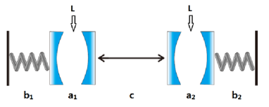
Figure 1: (Color online) Schematic setup of the model. The quantum state initially encoded on the mechanical mode 1 coupled to cavity 1 via radiation pressure is transferred to the mechanical mode 2 coupled to cavity 2 via radiation pressure. The state can be transferred completely without considering leakage rates $\kappa_{j}$ and ${\gamma_{j}}$.

In the interaction picture, the Hamiltonian of the system can be written as ^[18-21],

$$H{\rm{=}} {\omega_{\rm{m_{1}}}}b_{1}^{\dagger}{b_{1}}+{\omega_{\rm{m_{2}}}}b_{2}^{\dagger}{b_{2}}-{\Delta_{1}}a_{1}^{\dagger}{a_{1}}-{\Delta_{2}}a_{2}^{\dagger}{a_{2}}+{\omega_{c}}{c^{\dagger}}c$$ (1)

$$+g\left({a_{1}^{\dagger}c+a_{2}^{\dagger}c+{a_{1}}{c^{\dagger}}+{a_{2}}{c^{\dagger}}}\right)$$ (2)

$$+{G_{1}}\left({{a_{1}}b_{1}^{\dagger}+a_{1}^{\dagger}{b_{1}}}\right)+{G_{2}}\left({{a_{2}}b_{2}^{\dagger}+a_{2}^{\dagger}{b_{2}}}\right)\$$ (3)

where ${\omega_{\rm{m_{j}}}}$ is the frequency of the mechanical mode j, $b_{j}$ is the annihilation operator for the mechanical mode j, $a_{j}$ is the annihilation operator for the cavity mode j, ${\Delta_{j}}$ is the detuning of the optical drive applied to the cavity mode j, g is the coupling strength between the cavity and optical fiber, and $G_{j}$ is the coupling strength between the mechanical mode j and cavity j. Through the unitary transformation, we get the effective Hamiltonian of the system,

$$H^{\prime}{\rm{=}} {\omega_{\rm{m}}}b_{1}^{\dagger}{b_{1}}+{\omega_{\rm{m}}}b_{2}^{\dagger}{b_{2}}-\left({{\Delta_{1}}-\frac{{2{g^{2}}}}{\Delta}}\right)a_{1}^{\dagger}{a_{1}}$$ (4)

$$-\left({{\Delta_{2}}-\frac{{2{g^{2}}}}{\Delta}}\right)a_{2}^{\dagger}{a_{2}}+\left({{\omega_{c}}-\frac{{4{g^{2}}}}{\Delta}}\right){c^{\dagger}}c$$ (5)

$$+\frac{{2{g^{2}}}}{\Delta}\left({a_{1}^{\dagger}{a_{2}}+{a_{1}}a_{2}^{\dagger}}\right)+{G_{1}}\left({{a_{1}}b_{1}^{\dagger}+a_{1}^{\dagger}{b_{1}}}\right)$$ (6)

$$+{G_{2}}\left({{a_{2}}b_{2}^{\dagger}+a_{2}^{\dagger}{b_{2}}}\right)\$$ (7)

here we choose $U={e^{\frac{g}{\Delta}\left({a_{1}^{\dagger}c+a_{2}^{\dagger}c-{a_{1}}{c^{\dagger}}-{a_{2}}{c^{\dagger}}}\right)}}$, and $H^{\prime}=UH{U^{\dagger}}$. For easier calculation, we can choose ${\Delta_{1}}={\Delta_{2}}=-\Delta-{\omega_{c}}$, at the same time it's under the case of large detuning conditions, $\Delta>>g$. In the Heisenberg picture, using input-output theory, we obtain the quantum Langevin equations for the cavity and mechanical mode operators

$${{\dot{a}}_{1}}= i\left({{\Delta_{1}}-\frac{{2{g^{2}}}}{\Delta}}\right){a_{1}}-i{G_{1}}{b_{1}}-i\frac{{2{g^{2}}}}{\Delta}{a_{2}}-\frac{{{\kappa_{1}}}}{2}{a_{1}}$$ (8)

$$+\sqrt{{\kappa_{1}}}{a_{in,1}}$$ (9)

$${{\dot{a}}_{2}}= i\left({{\Delta_{2}}-\frac{{2{g^{2}}}}{\Delta}}\right){a_{2}}-i{G_{2}}{b_{2}}-i\frac{{2{g^{2}}}}{\Delta}{a_{1}}-\frac{{{\kappa_{2}}}}{2}{a_{2}}$$ (10)

$$+\sqrt{{\kappa_{2}}}{a_{in,2}}$$ (11)

$${{{\dot{b}}_{1}}=-i{\omega_{\rm{m}}}{b_{1}}-i{G_{1}}{a_{1}}-\frac{{{\gamma_{1}}}}{2}{b_{1}}+\sqrt{{\gamma_{1}}}{f_{1}}}$$ (12)

$${{{\dot{b}}_{2}}=-i{\omega_{\rm{m}}}{b_{2}}-i{G_{2}}{a_{2}}-\frac{{{\gamma_{2}}}}{2}{b_{2}}+\sqrt{{\gamma_{2}}}{f_{2}}}$$ (13)

where ${\kappa_{j}}$ is the damping rate of the cavity mode j, ${\gamma_{j}}$ is the damping rate of the mechanical oscillator mode j, ${f_{j}}$ is the noise operator for the mechanical oscillator bath j, while ${a_{in,j}}$ describes the quantum noise of the vacuum field incident on the cavity mode j. Under ideal conditions, we can choose ${\kappa_{1}}={\kappa_{2}}={\gamma_{1}}={\gamma_{2}}=0$. And only considering the interaction terms, we get the Langevin equations without dissipative terms.

$${{{\dot{a}}_{1}}=-i{G_{1}}{b_{1}}-i\frac{{2{g^{2}}}}{\Delta}{a_{2}}}$$ (14)

$${{{\dot{a}}_{2}}=-i{G_{2}}{b_{2}}-i\frac{{2{g^{2}}}}{\Delta}{a_{1}}}$$ (15)

$${{{\dot{b}}_{1}}=-i{G_{1}}{a_{1}}}$$ (16)

$${{{\dot{b}}_{2}}=-i{G_{2}}{a_{2}}}$$ (17)

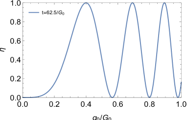
Figure 2: (Color online) The state transfer efficiency ${\eta}$ as a function of ${G_{0}}/{g_{0}}$ and for procedure time $t={20}/{g_{0}}$.

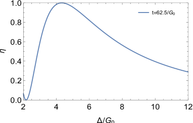
Figure 3: (Color online) The state transfer efficiency ${\eta}$ as a function of ${\Delta}/{g_{0}}$ and also for the time $t={20}/{g_{0}}$.

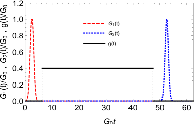
Figure 4: (Color online) The time profiles of the optomechanical coupling ${G_{1}}$ (red dashed curve), ${G_{2}}$ (blue dashed curve), and the coupling between cavity and optical fiber $g$ (black solid curve).

To analyze the quantum state transfer from mechanical oscillator mode 1 to mechanical oscillator mode 2, we use the corresponding classical equations for Eqs. (7)-(10):

$${{\alpha_{1}}=-i{G_{1}}{\beta_{1}}-i\frac{{2{g^{2}}}}{\Delta}{\alpha_{2}}}$$ (18)

$${{\alpha_{2}}=-i{G_{2}}{\beta_{2}}-i\frac{{2{g^{2}}}}{\Delta}{\alpha_{1}}}$$ (19)

$${{\beta_{1}}=-i{G_{1}}{\alpha_{1}}}$$ (20)

$${{\beta_{2}}=-i{G_{2}}{\alpha_{2}}}$$ (21)

We assume that only the mechanical oscillator mode 1 has excitation phonon at the initial moment. To solve the above equations numerically, we assume ${\beta_{1}}\left(0\right)=1,{\alpha_{1}}\left(0\right)=0,{\alpha_{2}}\left(0\right)=0$, ${\beta_{2}}\left(0\right)=0$, and the transfer efficiency of quantum state as $\eta={{{{\left|{{\beta_{2}}\left(t\right)}\right|}^{2}}}\mathord{\left/{\vphantom{{{{\left|{{\beta_{2}}\left(t\right)}\right|}^{2}}}{{{\left|{{\beta_{1}}\left(0\right)}\right|}^{2}}}}}\right.\kern-1.2pt}{{{\left|{{\beta_{1}}\left(0\right)}\right|}^{2}}}}$.

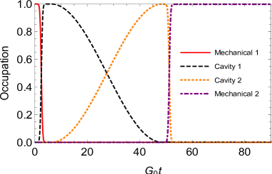
Figure 5: (Color online) Occupation number for the four modes. The quantum state is encoded on the first mechanical mode (red solid curve) and then transfer to the cavity 1 (black solid curve) and cavity 2 (blue dashed curve). At last, the quantum state is transferred to the mechanical mode 2 (purple solid curve) In the process, we make the center of Gaussian pulse at ${t_{1}}={1}/{g_{0}}$, ${t_{2}}={10}/{g_{0}}$ and $s=0.25/{g_{0}}$.

Before simulating evolution, we choose a Gaussian pulsed optomechanical coupling strength of the form ${G_{1}}\left(t\right)={G_{0}}{e^{{{-{{\left({t-{t_{1}}}\right)}^{2}}}\mathord{\left/{\vphantom{{-{{\left({t-{t_{1}}}\right)}^{2}}}{2{s^{2}}}}}\right.\kern-1.2pt}{2{s^{2}}}}}}$, ${G_{2}}\left(t\right)={G_{0}}{e^{{{-{{\left({t-{t_{2}}}\right)}^{2}}}\mathord{\left/{\vphantom{{-{{\left({t-{t_{2}}}\right)}^{2}}}{2{s^{2}}}}}\right.\kern-1.2pt}{2{s^{2}}}}}}$, where ${G_{0}}$ is the maximum optomechanical coupling strength, s is the width of the Gaussian pulses, and ${t_{i}}$ are the time at which the optomechanical coupling strength is maximum and the quantum state transfer from one mode to the other occurs. In addition, the form of the coupling strength between cavity and optical fiber is $g={g_{0}}$ when $t<9{g_{0}}$, and if ${t\geq 9{g_{0}}}$, then $g=0$.

From Fig.2-4, we obtain the procedure values of the maximum optomechanical coupling strength ${G_{0}}$ and detuning ${\Delta}$ which maximize the transfer efficiency ${\eta}$. The values are ${G_{0}}=2.5{g_{0}}$, $\Delta=10.5{g_{0}}$. In such a case, we can get a high transfer efficiency, just as shown in Fig. 5. When considering the dissipation ${\kappa}$ and ${\gamma}$, we get FIG. 6. Here the value of dissipations are ${\kappa_{1}}={\kappa_{2}}={\gamma_{1}}={\gamma_{2}}=0.01{g_{0}}$.

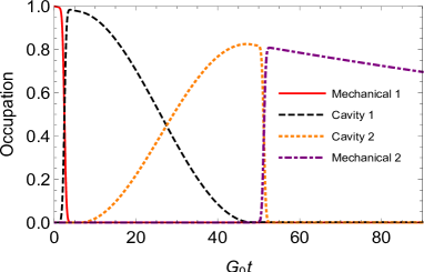
Figure 6: (Color online) Occupation number for the four modes. The quantum state is encoded on the first mechanical mode (red solid curve) and then transfer to the cavity 1 (black solid curve) and cavity 2 (blue dashed curve). At last, the quantum state is transferred to the mechanical mode 2 (purple solid curve) In the process, we also make the center of Gaussian pulse at ${t_{1}}={1}/{g_{0}}$, ${t_{2}}={10}/{g_{0}}$ and $s=0.25/{g_{0}}$.

Through analyzing the transfer of a quantum state between two distant mechanical oscillators which are separately coupled to two optical cavities, we get the optimal parameter solution for maximizing the transfer efficiency. In the process of analysis, we employed time-varying optomechanical coupling strength as a Gaussian pulsed. Choosing appropriate parameters, we got a high transfer efficiency, which is very closing to unity.

This work is supported by NSF of China under Grant No. 11305021 and the Fundamental Research Funds for the Central Universities under Grant Nos 3132015149 and 3032017072.

References

- (1) M. D. La Haye, O. Buu, B. Camarota, . Approaching the Quantum Limit of a Nanomechanical Resonator[J]. Science, 2004, 304(5667):74-77.
- (2) K. L. Ekinci, Y. T. Yang, M. L. Roukes. Ultimate limits to inertial mass sensing based upon nanoelectromechanical systems[J]. J. Appl. Phys. 2004, 95(5):2682.
- (3) K. C. Schwab, M. L. Roukes. Putting mechanics into quantum mechanics[J]. Phys.Today,2005, 58(7): 36-42.
- (4) D. Kleckner, D. Bouwmeester. Sub-kelvin optical cooling of a micromechanical resonator[J].Nature, 2006, 444(2):75-78.
- (5) O. Arcizet, P.-F. Cohadon, T. Briant, . Radiation-pressure cooling and optomechanical instability of a micromirror[J].Nature,2006, 444(2):71-74.
- (6) M. Poggio, C. L. Degen, H. J. Mamin, . Feedback cooling of a cantilever's fundamentalmode below 5 Mk[J]. Phys. Rev. Lett, 2007, 99(1):017201-017205.
- (7) M. Bhattacharya, P. Meystre. Trapping and Cooling a Mirror to Its Quantum Mechanical Ground State[J]. Phys. Rev. Lett. 2007, 99(7):073601(4).
- (8) T. Kazuyuki, N. Kentaro, N. Atsushi, Y. Rekishu, N. Yasunobu, I. Eiji, M. Jacob Taylor, U. Koji. Electro-mechano-optical NMR Detection. 2017, arXiv:1706.00532.
- (9) F. Massel, T. T. Heikkila, J. M. Pirkkalainen, S. U. Cho, H. Saloniemi, P. J. Hakonen, and M. A. Sillanpaa. Microwave ampli-fication with nanomechanical resonators. Nature (London), 2011, 480, 351.
- (10) X. Zhou, F. Hocke, A. Schliesser, A. Marx, H. Huebl, R. Gross and T. J. Kippenberg. Slowing, advancing and switching of microwave signals using circuit nanoelectromechanics, Nat. Phys. 2013, 9, 179.
- (11) A. J. Leggett. Testing the limits of quantum mechanics: motivation, state of play,prospects[J]. J. Phys: Condens. Matter, 2002, 14(15):R415.
- (12) W. Marshall, C. Simon, R. Penrose, . Towards Quantum Superpositions of a Mirror[J].Phys. Rev. Lett. 2003, 91(13): 130401(4).
- (13) T. J. Kippenberg, K. J. Vahala. Cavity Optomechanics:Back-Action at the Mesoscale[J].Science, 2008, 321(5893):1172-1176.
- (14) J. H. Teng. Theoretical Study of the Quantum Properties in Cavity Optomechanical System (Dalian University of Technology, 2014).
- (15) Wen-Zhao Zhang, Jiong Cheng and Ling Zhou. Quantum control gate in cavity optomechanical system. J. Phys. B: At. Mol. Opt. Phys. 2015, 48, 015502.
- (16) E. A. Sete and H. Eleuch. High-efficiency Quantum State Transfer and Quantum Memory Using a Mechanical Oscillator. Phy. Rev. A. 2015, 91, 032309.
- (17) K. Stannigel, P. Rabl, S. Rensen, . Optomechanical Transducers for Long-Distance Quantum Communication[J]. Phys. Rev. Lett, 2010, 105: 220501.
- (18) E. A. Sete and H. Eleuch. Interaction of a quantum well with squeezed light: Quantum-statistical properties. Phys. Rev. A. 2010, 82, 043810.
- (19) E. A. Sete, H. Eleuch, and S. Das. Semiconductor cavity QED with squeezed light: Nonlinear regime. Phys. Rev. A. 2011, 84, 053817.
- (20) E. A. Sete and H. Eleuch. Controllable nonlinear effects in an optomechanical resonator containing a quantum well. Phys. Rev. A. 2012, 85, 043824.
- (21) E. A. Sete and H. Eleuch. Light-to-matter entanglement transfer in optomechanics. J. Opt. Soc. Am. B. 2014, 31, 2821.