Assessment of the GLLB-SC potential for solid-state properties and attempts for improvement

Abstract

Based on the work of Gritsenko et al. (GLLB) [Phys. Rev. A 51, 1944 (1995)], the method of Kuisma et al. [Phys. Rev. B 82, 115106 (2010)] to calculate the band gap in solids was shown to be much more accurate than the common local density approximation (LDA) and generalized gradient approximation (GGA). The main feature of the GLLB-SC potential (SC stands for solid and correlation) is to lead to a nonzero derivative discontinuity that can be conveniently calculated and then added to the Kohn-Sham band gap for a comparison with the experimental band gap. In this work, a thorough comparison of GLLB-SC with other methods, e.g., the modified Becke-Johnson (mBJ) potential [F. Tran and P. Blaha, Phys. Rev. Lett. 102, 226401 (2009)], for electronic, magnetic, and density-related properties is presented. It is shown that for the band gap, GLLB-SC does not perform as well as mBJ for systems with a small band gap and strongly correlated systems, but is on average of similar accuracy as hybrid functionals. The results on itinerant metals indicate that GLLB-SC overestimates significantly the magnetic moment (much more than mBJ does), but leads to excellent results for the electric field gradient, for which mBJ is in general not recommended. In the aim of improving the results, variants of the GLLB-SC potential are also tested.

I Introduction

The great success of the Kohn-Sham (KS) density functional theory (DFT) method Hohenberg and Kohn (1964); Kohn and Sham (1965) for the calculation of properties of electronic systems is due to the fact that in many circumstances, results of sufficient accuracy can be obtained at much lower cost compared to the supposedly more reliable post-Hartree-FockJensen (2007) or Green’s function based methods.Bechstedt (2015) However, in KS-DFT the exchange (x) and correlation (c) effects are approximated and among the hundreds of approximations available,Marques et al. (2012) one has to choose an appropriate one for the system at hand. This choice is crucial when the trends in the results may depend significantly on the approximation, but the main problem is that it is by far not always obvious which approximation to choose. Therefore, the search for approximations that are more broadly accurate is a very active research topic, Kümmel and Kronik (2008); Cohen et al. (2012); Burke (2012); Becke (2014) in particular since KS-DFT is used in many areas of science.

The focus of the present work is on the properties which depend directly on the xc potential $v_{\text{xc},\sigma}$ ($\sigma$ is the spin index) in the KS equations, namely, the electronic structure, magnetic moment, and electron density. Given an xc energy functional $E_{\text{xc}}$, the variational principle requires $v_{\text{xc},\sigma}$ to be the functional derivative of $E_{\text{xc}}$. Depending on the type of approximation chosen for $E_{\text{xc}}$ and the way the functional derivative is taken (with respect to the electron density $\rho_{\sigma}$ or the orbitals $\psi_{i\sigma}$), the potential $v_{\text{xc},\sigma}$ can be of different nature: multiplicative or nonmultiplicative.Kümmel and Kronik (2008); Yang et al. (2012) Strictly speaking, the potential $v_{\text{xc},\sigma}$ in the KS method is multiplicative, while the generalized KS frameworkSeidl et al. (1996) (gKS) includes also nonmultiplicative potentials.

It is well-known that with the exact multiplicative potential, the KS band gap $E_{\text{g}}^{\text{KS}}$, defined as the conduction band minimum (CBM) minus the valence band maximum (VBM), is not equal to the true experimental (i.e., quasi-particle) band gap $E_{\text{g}}=I-A$ (ionization potential $I$ minus electron affinity $A$) since they differ by the so-called xc derivative discontinuity $\Delta_{\text{xc}}$,Perdew et al. (1982); Sham and Schlüter (1983)

$$E_{\text{g}}=E_{\text{g}}^{\text{KS}}+\Delta_{\text{xc}},$$ (1)

which can be of the same order of magnitude as the gap.Godby et al. (1986); Grüning et al. (2006, 2006); Klimeš and Kresse (2014) Since $\Delta_{\text{xc}}$ is positive, the exact KS gap $E_{\text{g}}^{\text{KS}}$ is (much) smaller than $E_{\text{g}}$. Therefore, within the KS framework a comparison with the experimental gap should formally be done only when $\Delta_{\text{xc}}$ is added to the KS band gap. With the functionals of the local density approximation (LDA) and generalized gradient approximation (GGA) that are commonly used for structure optimization or binding energy calculation (e.g., PBEPerdew et al. (1996)), $E_{\text{g}}^{\text{KS}}$ is usually much smaller than $E_{\text{g}}$ (see, e.g., Ref. Heyd et al., 2005), while adding $\Delta_{\text{xc}}$ (calculated in some way, which is possible for finite systemsAndrade and Aspuru-Guzik (2011); Chai and Chen (2013); Kraisler and Kronik (2014)) improves the agreement with experiment. Note that interestingly, the LDA and standard GGA methods lead to KS band gaps that do not differ that much from accurate KS band gaps.Godby et al. (1986); Grüning et al. (2006, 2006); Klimeš and Kresse (2014)

Semilocal multiplicative xc potentials that are more useful for band gap calculation have been proposed, Engel and Vosko (1993); Zhao et al. (1999); Becke and Johnson (2006); Tran et al. (2007); Ferreira et al. (2008); Tran and Blaha (2009); Armiento and Kümmel (2013); Singh et al. (2016); Finzel and Baranov (2017); Verma and Truhlar (2017); Morales-García et al. (2017) however since usually this is still $E_{\text{g}}^{\text{KS}}$ that is compared to the experimental value of $E_{\text{g}}$ (no $\Delta_{\text{xc}}$ added to $E_{\text{g}}^{\text{KS}}$), the better agreement is achieved at the cost of having a potential $v_{\text{xc}}$ that may show features that are most likely unphysical and not present in the exact KS potential (see, e.g., Fig. 2 of Ref. Tran and Blaha, 2017). Then, this may possibly lead to a bad description of properties other than the band gap. For instance, the modified Becke-Johnson (mBJ) potential,Tran and Blaha (2009) which has been very successful for band gap prediction,Singh (2010); Botana et al. (2012); Zhu and Schwingenschlögl (2012); Koller et al. (2012); Camargo-Martínez and Baquero (2012); Jiang (2013); Dixit et al. (2012); Waroquiers et al. (2013); Tran and Blaha (2017) has also shown to be sometimes rather inaccurate for other properties, e.g., band widthsWaroquiers et al. (2013) or the magnetic moment of itinerant metals.Koller et al. (2011) This is the consequence of constructing a potential that is not well-founded from the physical point of view.

Thus, when using a multiplicative potential the proper calculation of $E_{\text{g}}=I-A$ should consist of a nonzero derivative discontinuity that is added to $E_{\text{g}}^{\text{KS}}$ [Eq. (1)]. In Refs. Kuisma et al., 2010; Andrade and Aspuru-Guzik, 2011; Chai and Chen, 2013; Kraisler and Kronik, 2014, methods to calculate the derivative discontinuity were proposed, however among these works only the one from Kuisma et al.Kuisma et al. (2010) can be used for solids. They showed how to calculate the exchange part $\Delta_{\text{x}}$ of the derivative discontinuity from quantities that are obtained from a standard ground-state KS calculation. $\Delta_{\text{x}}$ is nonzero since they used a xc potential that is based on the one proposed by Gritsenko et al. (GLLB),Gritsenko et al. (1995, 1997) which exhibits a jump (step structure) when the lowest unoccupied orbital starts to be occupied. The GLLB potential is a simplified version of the Krieger-Li-Iafrate (KLI) approximation Krieger et al. (1992) to the optimized effective potential (OEP).Sharp and Horton (1953) The potential of Kuisma et al.,Kuisma et al. (2010) called GLLB-SC (SC for solid and correlation), has been shown to be much more accurate than LDA and standard GGA for the calculation of band gaps in solids (see Refs. Castelli et al., 2012; Yan et al., 2012; Hüser et al., 2013; Miró et al., 2014; Pilania et al., 2016; Kim et al., 2016; Pandey et al., 2017 for extensive tests) and to reach an accuracy similar to the $GW$ methods.Yan et al. (2012); Hüser et al. (2013)

Very recently,Pandey et al. (2017) GLLB-SC and mBJ band gaps of the chalcopyrite, kesterite, and wurtzite polymorphs of II-IV-V₂ and III-III-V₂ semiconductors were compared. It was shown that in most cases the GLLB-SC and mBJ band gaps are rather similar, however, in a few cases rather large differences were obtained. The experimental values were not known for a sufficient number of systems to draw a clear conclusion about the relative accuracy of the GLLB-SC and mBJ methods. To our knowledge, this is the only work which reports a direct comparison between the GLLB-SC method and other semilocal potentials that were also shown to be useful for band gap calculation in solids. The aim of the present work is to provide such a comparison, and for the band gap the large test set of 76 solids considered in our recent workTran and Blaha (2017) has been chosen. Since the band gap is obviously not the only interesting property of a solid to consider, results for ground-state quantities like electron densities, electric field gradients, and magnetic moments will also be shown and discussed.

The paper is organized as follows. In Sec. II, a description of the methods and the computational details are given. In Sec. III, the results are presented and discussed, and in Sec. IV the summary of the work is given.

II Methodology

We begin by describing briefly the GLLB method and its slightly modified version GLLB-SC. More details can be found in the original worksGritsenko et al. (1995, 1997); Kuisma et al. (2010) or in a recent review.Baerends (2017) The xc energy $E_{\text{xc}}$ can be expressed with the pair-correlation function and this leads naturally to the following partitioning for the functional derivative $v_{\text{xc},\sigma}=\delta E_{\text{xc}}/\delta\rho_{\sigma}$:

$$v_{\text{xc},\sigma}(\bm{r})=v_{\text{xc,hole},\sigma}(\bm{r})+v_{\text{xc,resp},\sigma}(\bm{r}),$$ (2)

where the first term is twice the xc energy density per particle, $v_{\text{xc,hole},\sigma}=2\varepsilon_{\text{xc},\sigma}=2\left(\varepsilon_{\text{x},\sigma}+\varepsilon_{\text{c}}\right)$ with $\varepsilon_{\text{x},\sigma}$ and $\varepsilon_{\text{c}}$ defined as

$$E_{\text{xc}}=\sum_{\sigma}\int\varepsilon_{\text{x},\sigma}(\bm{r})\rho_{\sigma}(\bm{r})d^{3}r+\int\varepsilon_{\text{c}}(\bm{r})\rho(\bm{r})d^{3}r,$$ (3)

and is called the hole term since it is the Coulomb potential produced by the xc hole. $v_{\text{xc,resp},\sigma}$ is the response term which accounts for the response of the pair correlation function to a variation in the electron density. The exchange part $v_{\text{x,hole},\sigma}$ of the hole term is the Slater potential,Slater (1951) i.e., twice the Hartree-Fock (HF) exchange energy density, which reduces to $\left(3/2\right)v_{\text{x},\sigma}^{\text{LDA}}$ for a constant electron density, where $v_{\text{x},\sigma}^{\text{LDA}}$ is the exchange potential for constant density [$v_{\text{x,resp},\sigma}$ reduces to $-\left(1/2\right)v_{\text{x},\sigma}^{\text{LDA}}$ such that overall Eq. (2) recovers the LDA limit for constant density].

Neglecting correlation, Gritsenko et al.Gritsenko et al. (1995) proposed two exchange potentials based on the partitioning given by Eq. (2) which differ by the hole term. Their first potential uses the exact (i.e., Slater) hole term, while the second one uses the exchange energy density of the B88 GGA functionalBecke (1988) ($v_{\text{x,hole},\sigma}^{\text{B88}}=2\varepsilon_{\text{x},\sigma}^{\text{B88}}$). For both potentials the exchange response term is given by

$$v_{\text{x,resp},\sigma}^{\text{GLLB}}(\bm{r})=K_{\text{x}}\sum_{i=1}^{N_{\sigma}}\sqrt{\epsilon_{\text{H}}-\epsilon_{i\sigma}}\frac{\left|\psi_{i\sigma}(\bm{r})\right|^{2}}{\rho_{\sigma}(\bm{r})},$$ (4)

where the sum runs over the $N_{\sigma}$ occupied orbitals of spin $\sigma$, $\epsilon_{\text{H}}$ is the highest (H) occupied orbital, and $K_{\text{x}}$ was either chosen to be $K_{\text{x}}^{\text{LDA}}=8\sqrt{2}/\left(3\pi^{2}\right)$ in order to satisfy the correct LDA limit for constant electron density or determined to satisfy the virial relation for exchange.Levy and Perdew (1985) Eq. (4) is a simplified and computationally faster version of the KLIKrieger et al. (1992) response term.Gritsenko et al. (1995); Kohut et al. (2014) In a subsequent work,Gritsenko et al. (1997) correlation was also included in the GLLB potential. For the hole term this was done by adding $v_{\text{c,hole}}^{\text{PW91}}=2\varepsilon_{\text{c}}^{\text{PW91}}$ (PW91 is the GGA from Perdew and WangPerdew et al. (1992)), while for the response term $K_{\text{x}}$ was replaced by $K_{\text{xc}}$ that was determined from different schemes, e.g., satisfying the virial relation for exchange and correlation.

The GLLB-SC potentialKuisma et al. (2010) uses the GGA PBEsolPerdew et al. (2008) for the exchange hole term, but also for the total (hole plus response) correlation:

$$v_{\text{xc},\sigma}^{\text{GLLB-SC}}(\bm{r}) = 2\varepsilon_{\text{x},\sigma}^{\text{PBEsol}}(\bm{r})$$ (5)

$$+K_{\text{x}}^{\text{LDA}}\sum_{i=1}^{N_{\sigma}}\sqrt{\epsilon_{\text{H}}-\epsilon_{i\sigma}}\frac{\left|\psi_{i\sigma}(\bm{r})\right|^{2}}{\rho_{\sigma}(\bm{r})}$$

$$+v_{\text{c},\sigma}^{\text{PBEsol}}(\bm{r}),$$

where $v_{\text{c},\sigma}^{\text{PBEsol}}=\delta E_{\text{c}}^{\text{PBEsol}}/\delta\rho_{\sigma}$ is the total (hole plus response) correlation potential.

The most important feature of the GLLB(-SC) potentials is to vary abruptly when the lowest (L) unoccupied orbital ($\psi_{\text{L}}$) starts to be occupied by an infinitesimal amount $\delta$ and leads to the replacement of $\epsilon_{\text{H}}$ by $\epsilon_{\text{L}}$ in Eq. (4). This is the so-called step structure that is also exhibited by the exact xc potential, but not by most LDA and GGA potentials. The BJ Becke and Johnson (2006); Armiento et al. (2008) and Armiento-KümmelArmiento and Kümmel (2013) potentials are examples of semilocal potentials that show such step structure. Kuisma et al.Kuisma et al. (2010) showed that the step structure of the GLLB(-SC) potential leads to an expression for the exchange component of the derivative discontinuity that is given by (see Ref. Baerends, 2017 for a detailed derivation)

$$\Delta_{\text{x}}^{\text{GLLB(-SC)}} = \int\psi_{\text{L}}^{*}(\bm{r})\left[\sum_{i=1}^{N_{\sigma_{\text{L}}}}K_{\text{x}}^{(\text{LDA})}\left(\sqrt{\epsilon_{\text{L}}-\epsilon_{i\sigma_{\text{L}}}}\right.\right.$$

$$-\left.\left.\sqrt{\epsilon_{\text{H}}-\epsilon_{i\sigma_{\text{L}}}}\right)\frac{\left|\psi_{i\sigma_{\text{L}}}(\bm{r})\right|^{2}}{\rho_{\sigma_{\text{L}}}(\bm{r})}\right]\psi_{\text{L}}(\bm{r})d^{3}r,$$

(6)

where $\sigma_{\text{L}}$ is the spin of $\psi_{\text{L}}$ and the integration is performed in the unit cell. It should be noted that in the case of metals, i.e., when $\epsilon_{\text{H}}=\epsilon_{\text{L}}$, Eq. (6) is zero, and therefore if Eq. (5) falsely predicts a system to be metallic (e.g., for InSb or FeO, see Sec. III), then Eq. (6) is of no use.

As underlined in Sec. I, the formally correct way to calculate the true band gap within the KS theory is to add a discontinuity to the KS band gap, and this is what is done with the GLLB(-SC) method. This is the very nice feature of GLLB(-SC), but it is also clear that this method is only half satisfying since the discontinuity is calculated only for exchange. In principle correlation effects should be much smaller than exchange, however it was shown that the xc discontinuity $\Delta_{\text{xc}}$ calculated in the random phase (RPA) OEP approximation for correlationGrüning et al. (2006); Klimeš and Kresse (2014) is much smaller (by at least 50%) than $\Delta_{\text{x}}$ calculated with exact exchange (EXX) OEP. Therefore, agreement with experiment for the band gap can still not be fully justified from the formal point of view with GLLB(-SC).

For the present work, the GLLB-SC potential and its associated derivative discontinuity, Eqs. (5) and (6), have been implemented in WIEN2k,Blaha et al. (2001) which is an all-electron code based on the linearized augmented plane-wave method.Andersen (1975); Singh and Nordström (2006) From the technical point of view, we only mention that the sums in Eqs. (5) and (6) include both the band and core electrons. The results of calculations with the GLLB-SC potential on various properties will be compared to those obtained with other multiplicative potentials of the LDA, GGA, or meta-GGA (MGGA) type, which are the following. The LDAKohn and Sham (1965); Perdew and Wang (1992) is exact for the homogenous electron gas, while Sloc (abbreviation for local Slater potentialFinzel and Baranov (2017)) consists of an enhanced exchange LDA (compare $v_{\text{x},\sigma}^{\text{Sloc}}=-1.67\left(2\rho_{\sigma}\right)^{0.3}$ to $v_{\text{x},\sigma}^{\text{LDA}}\simeq-0.7386\left(2\rho_{\sigma}\right)^{1/3}$) with no correlation added. The GGAs are the xc PBE from Perdew et al.,Perdew et al. (1996) the exchange of Engel and Vosko Engel and Vosko (1993) (EV93PW91, combined with PW91 correlationPerdew et al. (1992) as done previously in Ref. Tran et al., 2007), the exchange from Armiento and KümmelArmiento and Kümmel (2013); Vlček et al. (2015); Lindmaa and Armiento (2016) (AK13, no correlation added as done in Refs. Armiento and Kümmel, 2013; Vlček et al., 2015), and HLE16Verma and Truhlar (2017) which is a modification of HCTH/407Boese and Handy (2001) (the exchange and correlation components are multiplied by 1.25 and 0.5, respectively). Note that all GGA potentials depend on $\rho_{\sigma}$ and its first two derivatives, while the xc potential LB94 of van Leeuwen and Baerends,van Leeuwen and Baerends (1994) also considered in the present work, depends only on $\rho_{\sigma}$ and its first derivative. Therefore, LB94 is neither a LDA nor a GGA, but lies in between (note that correlation in LB94 is LDAPerdew and Wang (1992)). The tested MGGA are the aforementioned BJBecke and Johnson (2006) and mBJTran and Blaha (2009) potentials that are both combined with LDA for correlationPerdew and Wang (1992) (BJLDA and mBJLDA). Note that the LDA and GGA potentials are obtained as functional derivative $v_{\text{xc},\sigma}=\delta E_{\text{xc}}/\delta\rho_{\sigma}$ of energy functionals, while this is not the case for the GLLB-SC, LB94, and (m)BJLDA potentials.Karolewski et al. (2009); Gaiduk and Staroverov (2009); Karolewski et al. (2013) We also mention that among these potentials, (m)BJLDA, AK13, and LB94 were recently shown to lead to severe numerical problems in finite systems.Aschebrock et al. (2017a, b)

For completeness, calculations with a hybrid functional, YS-PBE0,Tran and Blaha (2011) were also done. In YS-PBE0 (YS stands for Yukawa screened), the Coulomb operator in the HF exchange is exponentially screened (i.e., Yukawa potential) and it was shownTran and Blaha (2011) (see also Ref. Shimazaki and Asai, 2008) that YS-PBE0 leads to the same band gaps as the popular HSE06 from Heyd, Scuseria, and ErnzerhofHeyd et al. (2003); Krukau et al. (2006) which uses an error-function for the screening of the HF exchange. In the following, the acronym HSE06 will be used for all results that were obtained with YS-PBE0. Since hybrid functionals contain a fraction of HF exchange,Becke (1993) (25% in YS-PBE0/HSE06) that is usually implemented in the gKS framework (as done in WIEN2kTran and Blaha (2011)), the potential is nonmultiplicative. With nonmultiplicative potentials (a part of) the discontinuity $\Delta_{\text{xc}}$ is included in the orbital energies,Yang et al. (2012); Perdew et al. (2017) which means that the gap CBM minus VBM should in principle be in better agreement with the experimental gap $E_{\text{g}}$. However, note that hybrid functionals are much more expensive than semilocal functionals such that they can not be applied routinely to very large systems, in particular with codes based on plane-waves basis functions.

All calculations presented in this work were done with WIEN2k and the convergence parameters of the calculations, like the size of the basis set or the number of $\bm{k}$-points for the integrations in the Brillouin zone, were chosen such that the results are well converged (e.g., within $\sim 0.03$ eV for the band gap). The solids of the test sets are listed in Table S1 of the Supplemental Material,SM_ along with their space group and experimental geometry that was used for the calculations. For most calculations, the deep-lying core states (those which are below the Fermi energy by at least $\sim 6$ Ry) were treated fully relativistically, i.e., by including spin-orbit coupling (SOC), while the band states (semicore, valence, and unoccupied) were treated at the scalar-relativistic level. The only exceptions are the results for the effective masses of III-V semiconductors, which were obtained with SOC included also for the band electrons in a second-variational step.Koelling and Harmon (1977); MacDonald et al. (1980)

III Results and discussion

III.1 Electronic structure

Table 1: Summary statistics for the error in the calculated band gaps in Table S2 of the Supplemental MaterialSM_ for the set of 76 solids. M(R)E, MA(R)E, and STD(R)E denote the mean (relative) error, the mean absolute (relative) error, and the standard deviation of the (relative) error, respectively. The calculations were done at the experimental geometry specified in Table S1 of the Supplemental Material.SM_ All results except those obtained with the BJLDA, LB94, and GLLB-SC methods are taken from Ref. Tran and Blaha, 2017.

	LDA	PBE	EV93PW91	AK13	Sloc	HLE16	BJLDA	mBJLDA	LB94	GLLB-SC	HSE06
ME (eV)	-2.17	-1.99	-1.55	-0.28	-0.76	-0.82	-1.53	-0.30	-1.87	0.20	-0.68
MAE (eV)	2.17	1.99	1.55	0.75	0.90	0.90	1.53	0.47	1.88	0.64	0.82
STDE (eV)	1.63	1.56	1.55	0.89	0.93	1.07	1.24	0.57	1.23	0.81	1.21
MRE (%)	-58	-53	-35	-6	-21	-20	-41	-5	-54	-4	-7
MARE (%)	58	53	36	24	30	25	41	15	55	24	17
STDRE (%)	23	23	23	31	37	28	22	22	29	34	22

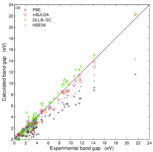
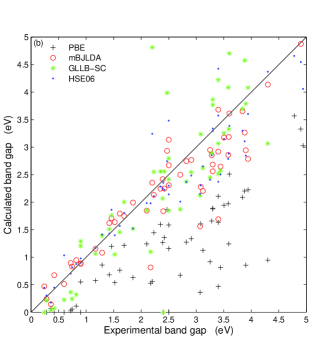
Figure 1: Calculated versus experimental fundamental band gaps for the set of 76 solids. The values are given in Table S2 of the Supplemental Material.SM_ The lower panel is a zoom of the upper panel focusing on band gaps smaller than 5 eV.

We start the discussion of the results with the fundamental band gap, whose values are shown in Table S2 of the Supplemental MaterialSM_ for the 76 solids of our test set, which are of various types: $sp$-semiconductors, ionic insulators, rare gases, and strongly correlated solids. The contribution of the exchange discontinuity $\Delta_{\text{x}}$ to the GLLB-SC band gap is indicated in parenthesis. The summary statistics for the error is given in Table 1. Note that the results obtained with all methods except BJLDA, LB94, and GLLB-SC are from Ref. Tran and Blaha, 2017. The worst agreements with experiment are obtained with the standard LDA and PBE, as well as with LB94 (LB94$\alpha$Schipper et al. (2000) leads to quite similar results on average), which strongly underestimate the band gap and lead to MAE and MARE around 2 eV and $55\%$, respectively, while EV93PW91 and BJLDA are slightly more accurate. Much better results are obtained with the other methods, since the MAE (MARE) of AK13, Sloc, HLE16, GLLB-SC, and the hybrid HSE06 are in the range 0.64-0.90 eV (17-30%). However, the best agreement with experiment is obtained with the mBJLDA potential, which leads to the smallest MAE (0.47 eV) and MARE (15%). As discussed in Refs. Tran and Blaha, 2009; Koller et al., 2011; Tran and Blaha, 2017, the very good performance of the mBJLDA potential can be attributed to its dependency on two ingredients: the kinetic-energy density $t_{\sigma}=\left(1/2\right)\sum_{i=1}^{N_{\sigma}}\nabla\psi_{i\sigma}^{*}\cdot\nabla\psi_{i\sigma}$, which seems particularly important for solids with strongly correlated $3d$-electrons, and the average of $\nabla\rho/\rho$ in the unit cell that is able to somehow account for screening effects (see the discussion on metals in Sec. III).

The band gaps calculated with the GLLB-SC method, which consist of the sum of the KS band gap (CBM minus VBM) and the exchange discontinuity [Eq. (6)] are pretty accurate in most cases. Indeed, the MAE of 0.64 eV is smaller than the value for the hybrid functional HSE06 (and also B3PW91 which leads to 0.73 eVTran and Blaha (2017)), and only mBJLDA has a smaller MAE. The MARE is 24%, which is a rather fair value in comparison to the other methods, since it is similar to the values for the GGAs AK13 and HLE16, but larger than what mBJLDA and HSE06 give. The ME and MRE, which are the smallest among all tested methods, indicate that GLLB-SC shows the least pronounced tendency to underestimate or overestimate the band gaps on average. However, by looking at Fig. 1, which shows graphically the band gaps for a few selected methods, we can see that there is a noticeable tendency to underestimate many of the band gaps smaller than 3 eV, while an overestimation is observed for band gaps larger than 4 eV. This is more or less the opposite of what is observed for mBJLDA, as seen in Fig. 1.

The main conclusion from the statistics in Table 1 for the band gap is that mBJLDA is more accurate than GLLB-SC, since the most important quantities, the MAE and MARE, are the smallest, which is also the case for the STDE and STDRE. The GLLB-SC results should also be considered as very good since the overall performance is very similar to hybrid functionals. However, note that there are some cases where GLLB-SC gives a band gap that is clearly too small, and from Fig. 1 and Table S2 we can see that this concerns mainly band gaps that are (experimentally) below 1 eV and FeO. The worst cases are InAs, InSb, SnTe, and FeO that are described as (nearly) metallic by GLLB-SC, which is in contradiction with experiment, while mBJLDA leads to reasonably good results.

Concerning the strongly correlated solids, which are known to be very difficult cases for the standard functionals,Terakura et al. (1984) the GLLB-SC results seem to be particularly disparate. For Cr₂O₃, MnO, and CoO the agreement with experiment is very good. However, as mentioned above, GLLB-SC leads to no gap in FeO (from experiment it should be around 2.4 eV) and in NiO there is an underestimation of more than 1 eV. On the other hand, the gap is 4.81 eV in Fe₂O₃, which is too large by 2.6 eV and should be the consequence of an exchange splitting that is too large (as shown in Sec. III.2, the magnetic moments of metals are by far overestimated). The mBJLDA potential leads to much more consistent results, since the largest discrepancy is an underestimation of about 1 eV for MnO. As mentioned in Ref. Tran and Blaha, 2017, all LDA and GGA methods lead to severely underestimated band gaps for the strongly correlated solids, the only exception being Sloc for MnO. LB94 is even worse since no band gap is obtained for most strongly correlated solids.

On the other hand, in Ref. Tran and Blaha, 2017 we underlined that mBJLDA underestimates by a rather large amount (1-1.7 eV, see Table S2) the band gap of the Cu¹⁺ compounds, with CuCl being one of the worst case. For these systems, the GLLB-SC band gaps are, with respect to mBJLDA, larger by 0.3-1.3 eV such that the agreement with experiment is improved. However, with the exception of CuSCN, a sizeable underestimation is still obtained.

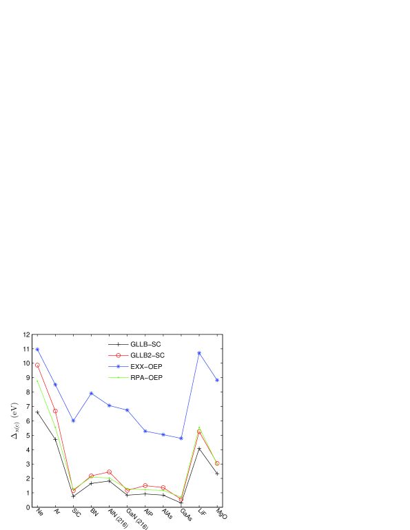
Figure 2: GLLB-SC and GLLB2-SC derivative discontinuities compared to the values calculated in the framework of the EXX-OEP and RPA-OEP methods.Klimeš and Kresse (2014)

Discussing now the derivative discontinuity $\Delta_{\text{x}}^{\text{GLLB-SC}}$, Table S2 shows that its contribution to the total GLLB-SC band gap is in the range 25-35% for most solids, which is rather substantial. Without $\Delta_{\text{x}}^{\text{GLLB-SC}}$, the GLLB-SC band gaps would be still larger than the PBE band gaps, but clearly smaller than experiment. In Ref. Klimeš and Kresse, 2014, discontinuities were calculated in the framework of the EXX-OEP and RPA-OEP methods, and it was shown that the sum of the RPA-OEP KS band gap and $\Delta_{\text{xc}}^{\text{RPA-OEP}}$ is in relatively fair agreement with the experimental band gap for many of the solids that were considered. Thus, the order of magnitude of $\Delta_{\text{xc}}^{\text{RPA-OEP}}$ should be similar to the exact one in those cases where agreement with experiment is good. Figure 2 compares the discontinuities calculated with the GLLB-SC and OEP methods, and one can clearly see that the GLLB-SC values are much closer to RPA-OEP than to EXX-OEP, despite the fact that $\Delta_{\text{x}}^{\text{GLLB-SC}}$ is supposed to be only for exchange. We can also see that $\Delta_{\text{x}}^{\text{GLLB-SC}}$ is smaller than $\Delta_{\text{xc}}^{\text{RPA-OEP}}$ by 0.2-2 eV. For the sake of consistency, it would be more preferable to have agreement with $\Delta_{\text{xc}}^{\text{RPA-OEP}}$ with a GLLB-type discontinuity which also includes correlation. As mentioned in the introduction, a (conveniently easy) way to do it was proposed in Ref. Gritsenko et al., 1997, and we followed a similar strategy for the construction of a potential, called GLLB2-SC, that also includes correlation in the discontinuity (see Sec. III.5.2 for details). The values of $\Delta_{\text{xc}}^{\text{GLLB2-SC}}$, also shown in Fig. 2, show a surprisingly nice agreement with the RPA-OEP values for most solids. The largest difference between $\Delta_{\text{xc}}^{\text{GLLB2-SC}}$ and $\Delta_{\text{xc}}^{\text{RPA-OEP}}$ are found for Ne and Ar, and are about 1 eV. Nevertheless, we do not expect such a good agreement for strongly correlated systems, since in the case of FeO, for instance, the KS band gap, and therefore the discontinuity, is still zero with GLLB2-SC. Furthermore, as discussed later in Sec. III.5.2, the band gaps with GLLB2-SC are much less accurate than with the original GLLB-SC potential, such that GLLB2-SC is not really interesting for band gap calculation.

Table 2: Effective hole and electron masses at the $\Gamma$ point in units of the electron rest mass ${m_{e}}$ calculated along the $\Gamma$X [100] direction. The calculations were done at the experimental geometry (see Table S1 of the Supplemental MaterialSM_ ) and include SOC. The experimental values were calculated from the Luttinger parameters tabulated in Ref. Vurgaftman et al., 2001. The values which agree the best (worst) with experiment are in bold (underlined). In some cases, because the shape of the band at $\Gamma$ is of nonparabolic type, the effective mass can not be calculated.

Solid	Method	$\left|m^{*}_{\text{split-off}}/m_{e}\right|$	$\left|m^{*}_{\text{light-hole}}/m_{e}\right|$	$\left|m^{*}_{\text{heavy-hole}}/m_{e}\right|$	$\left|m^{*}_{\text{electron}}/m_{e}\right|$
InP	LDA	0.095	0.051	0.404	0.036
	PBE	0.127	0.073	0.418	0.052
	EV93PW91	0.200	0.128	0.453	0.096
	AK13	0.250	0.170	0.489	0.138
	Sloc	0.133	0.070	0.600	0.050
	HLE16	0.212	0.130	0.538	0.097
	BJLDA	0.150	0.086	0.427	0.065
	mBJLDA	0.231	0.153	0.476	0.115
	LB94	0.030		0.408	0.049
	GLLB-SC	0.174	0.107	0.442	0.079
	Expt.	0.210	0.121	0.531	0.080
InAs	LDA	0.028		0.317	0.062
	PBE			0.324	0.036
	EV93PW91	0.094	0.027	0.344	0.022
	AK13	0.148	0.062	0.387	0.049
	Sloc	0.026		0.472	0.062
	HLE16	0.081	0.012	0.417	0.011
	BJLDA	0.023		0.337	0.023
	mBJLDA	0.132	0.053	0.368	0.041
	LB94	0.104		0.338	0.200
	GLLB-SC	0.049		0.354
	Expt.	0.140	0.027	0.333	0.026
InSb	LDA	0.014		0.225	0.056
	PBE	0.044	0.111	0.200	0.036
	EV93PW91	0.097		0.213
	AK13	0.120	0.024	0.230	0.022
	Sloc	0.030		0.305	0.094
	HLE16	0.069	0.031	0.267	0.023
	BJLDA	0.048	0.080	0.211	0.034
	mBJLDA	0.114	0.020	0.229	0.018
	LB94	0.086		0.205	0.213
	GLLB-SC	0.060	0.033	0.210	0.023
	Expt.	0.110	0.015	0.263	0.014
GaAs	LDA	0.083	0.018	0.331	0.015
	PBE	0.111	0.039	0.335	0.031
	EV93PW91	0.169	0.083	0.348	0.067
	AK13	0.200	0.107	0.371	0.088
	Sloc	0.066		0.481
	HLE16	0.165	0.072	0.421	0.057
	BJLDA	0.135	0.056	0.351	0.044
	mBJLDA	0.212	0.118	0.379	0.094
	LB94	0.055		0.355	0.107
	GLLB-SC	0.136	0.057	0.358	0.045
	Expt.	0.172	0.090	0.350	0.067
GaSb	LDA	0.057	0.045	0.206	0.028
	PBE	0.079	0.100	0.207	0.009
	EV93PW91	0.120	0.029	0.214	0.026
	AK13	0.136	0.040	0.228	0.036
	Sloc	0.011	0.014	0.313	0.074
	HLE16	0.101		0.267
	BJLDA	0.093		0.219
	mBJLDA	0.148	0.051	0.235	0.045
	LB94	0.074		0.219	0.188
	GLLB-SC	0.089		0.213
	Expt.	0.120	0.044	0.250	0.039

Table 2 shows the effective hole and electron masses of zinc-blende III-V semiconductors calculated at $\Gamma$ along the $\Gamma$X [100] direction in the Brillouin zone. These semiconductors are those that we considered in Ref. Kim et al., 2010 to compare the accuracy of various methods for effective masses. The first observation that can be made about the present results is that there is no potential which is systematically among the best ones for all systems. Nevertheless, it is still possible to make a distinction between the most and least accurate methods. By considering the number of values which show the best and worst agreement with experiment (the values in bold and underlined, respectively), as well as the cases where the effective mass can not be calculated (when the band at $\Gamma$ is of nonparabolic type), the most reliable methods are EV93PW91 (11 accurate and 2 non-calculable), mBJLDA (7 accurate), HLE16 (9 accurate and 2 non-calculable), and AK13 (5 accurate and 1 inaccurate). EV93PW91 is particularly good for InP, InAs, and GaAs, HLE16 for InP, while mBJLDA and AK13 are very accurate for InSb and GaSb.

The other potentials are less accurate since as indicated in Table 2, there is a (much) larger number of cases where either the value is very inaccurate or can not be calculated. For instance, in the case of the GLLB-SC potential there are 3 accurate values, 1 inaccurate, and 4 that can not be calculated. The large errors usually correspond to underestimations at the split-off-hole and light-hole VBM, while no particular trend is observed for the heavy-hole VBM and electron CBM.

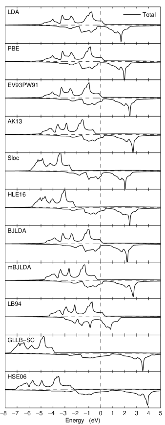
Figure 3: Calculated spin-up (upper curve) and spin-down (lower curve) total DOS of ferromagnetic Fe. The Fermi energy is set at zero.

To finish the discussion about the electronic structure, we show in Fig. 3 the density of states (DOS) of the ferromagnetic metal Fe. Compared to the case of $3d$ transition-metal oxides discussed above, the LDA and standard GGAs should be more reliable for itinerant transition metals where the $3d$ electrons are weakly correlated. In the case of Fe, the DOS obtained with LDA was shown to be in rather good agreement with experiment (spin-resolved X-ray photoelectron spectroscopySee and Klebanoff (1995)) for the valence band, and the same can be said for the PBE DOS which differs very little from the LDA DOS. However, the DOS obtained with some of the other methods differ substantially from the LDA/PBE DOS. The largest differences are obtained with GLLB-SC and HSE06, which lead to severely overestimated exchange splittings as shown in Fig. 3 and, consequently, to magnetic moments that are by far too large (see Sec. III.2). The overestimation of the exchange splitting is also very large with the Sloc and HLE16 potentials. The results for Co and Ni are quite similar with an exchange splitting that is the largest with GLLB-SC and HSE06. The failure of hybrid functionals for Fe, Co, and Ni has already been pointed out in recent studies.Paier et al. (2006); Jang and Yu (2012); Janthon et al. (2014); Gao et al. (2016)

III.2 Magnetism

Table 3: Calculated atomic spin magnetic moment $\mu_{S}$ (in $\mu_{\text{B}}$) of antiferromagnetic $3d$-transition metal oxides compared to experimental values of the total atomic magnetic moment $\mu_{S}+\mu_{L}$. The orbital moment $\mu_{L}$ is estimated to be in the range 0.6-1 $\mu_{\text{B}}$ for FeO, Svane and Gunnarsson (1990); Tran et al. (2006); Radwanski and Ropka (2008); Schrön and Bechstedt (2013) 1-1.6 $\mu_{\text{B}}$ for CoO, Svane and Gunnarsson (1990); Solovyev et al. (1998); Shishidou and Jo (1998); Neubeck et al. (2001); Jauch and Reehuis (2002); Ghiringhelli et al. (2002); Radwanski and Ropka (2004); Tran et al. (2006); Radwanski and Ropka (2008); Boussendel et al. (2010); Schrön and Bechstedt (2013) 0.3-0.45 $\mu_{\text{B}}$ for NiO,Svane and Gunnarsson (1990); Fernandez et al. (1998); Neubeck et al. (2001); Radwanski and Ropka (2004, 2008) and much smaller in other systems. The values of $\mu_{S}$ are those inside the atomic sphere of radius (in bohr) 2.02 (MnO), 2.00 (FeO), 2.00 (CoO), 1.92 (NiO), 1.97 (CuO), 1.94 (Cr₂O₃), and 1.96 (Fe₂O₃) of the transition-metal atom. The calculations were done at the experimental geometry specified in Table S1 of the Supplemental Material.SM_

Method	MnO	FeO	CoO	NiO	CuO	Cr2O3	Fe2O3
LDA	4.11	3.33	2.36	1.21	0.12	2.36	3.34
PBE	4.17	3.39	2.43	1.38	0.38	2.44	3.53
EV93PW91	4.24	3.44	2.49	1.47	0.46	2.53	3.71
AK13	4.39	3.51	2.59	1.57	0.54	2.68	3.93
Sloc	4.55	3.59	2.53	1.40	0.32	3.11	3.97
HLE16	4.51	3.62	2.59	1.48	0.40	2.96	4.02
BJLDA	4.19	3.40	2.48	1.48	0.50	2.43	3.59
mBJLDA	4.41	3.58	2.71	1.75	0.74	2.60	4.09
LB94	3.93	3.02	1.75	0.67	0.00	2.27	1.50
GLLB-SC	4.56	3.74	2.73	1.65	0.55	2.99	4.43
HSE06	4.36	3.55	2.65	1.68	0.67	2.61	4.08
Expt.	4.58	3.32,4.2,4.6	3.35,3.8,3.98	1.9,2.2	0.65	2.44,2.48,2.76	4.17,4.22

Turning now to the magnetic properties of systems with $3d$ electrons, Table 3 shows the atomic spin magnetic moment $\mu_{S}$ in antiferromagnetic transition-metal oxides. The comparison with experiment should be done by keeping in mind that there is a non-negligible orbital contribution $\mu_{L}$ for FeO, CoO, and NiO (see caption of Table 3).

In addition of being particularly inaccurate to describe the electronic structure of strongly correlated solids, the LDA and commonly used GGAs like PBE also lead to magnetic moments that are too small for this class of solids. Terakura et al. (1984); Dufek et al. (1994) DFT+$U$Anisimov et al. (1991) and the hybrid functionalsBredow and Gerson (2000); de P. R. Moreira et al. (2002); Franchini et al. (2005); Tran et al. (2006); Marsman et al. (2008) lead to much improved results and are therefore commonly used nowadays for such systems. However, those multiplicative potentials which are more accurate than LDA/PBE for the band gap also improve the results for the magnetic moment in most cases. From Table 3 we can see that in most cases, all tested potentials except LB94 increase the value of $\mu_{S}$ compared to LDA/PBE. EV93PW91 and BJLDA lead to moments which are only moderately larger, and AK13, Sloc, and HLE16 further improve the results, but the agreement with experiment is still not always satisfying. For instance, AK13 leads to a moment that is too small by 0.2 $\mu_{\text{B}}$ in MnO, while too large values are obtained with Sloc and HLE16 in the case of Cr₂O₃. GLLB-SC is pretty accurate for all monoxides, but less for Cr₂O₃ and Fe₂O₃ since the moments are overestimated by at least 0.2 $\mu_{\text{B}}$. Overall, the most reliable multiplicative potential seems to be mBJLDA, since it is the only one which leads to an error in the magnetic moment that should be below $\sim 0.2$ $\mu_{\text{B}}$ when a quantitative comparison with experiment is possible. As already pointed out in Ref. Koller et al., 2011, the moment of CuO obtained with mBJLDA is too large by at least 0.1 $\mu_{\text{B}}$. Furthermore, we note that for most systems the mBJLDA results are very close to the results obtained with HSE06. The worst results are obtained with LB94 which leads to the smallest magnetic moments in all cases.

Table 4: Calculated unit cell spin magnetic moment $\mu_{S}$ (in $\mu_{\text{B}}$/atom) of $3d$-transition metals. The experimental values are also spin magnetic moments. The calculations were done at the experimental geometry specified in Table S1 of the Supplemental Material.SM_

Method	Fe	Co	Ni
LDA	2.21	1.59	0.61
PBE	2.22	1.62	0.64
EV93PW91	2.48	1.68	0.68
AK13	2.58	1.70	0.69
Sloc	2.69	1.63	0.50
HLE16	2.72	1.72	0.63
BJLDA	2.39	1.63	0.62
mBJLDA	2.51	1.69	0.73
LB94	2.02	1.39	0.41
GLLB-SC	3.08	1.98	0.81
HSE06	2.79	1.90	0.88
Expt.	1.98,2.05,2.08	1.52,1.58,1.55-1.62	0.52,0.55

We also calculated the unit cell spin magnetic moment of the ferromagnetic metals Fe, Co, and Ni, and Table 4 shows the results that are compared with experimental values that do not include the orbital component $\mu_{L}$. It is well known that the simple LDA is relatively accurate for the magnetic moment of itinerant metals, while the trend of standard GGAs is to slightly overestimate the values (see Refs. Barbiellini et al., 1990; Singh et al., 1991; Leung et al., 1991; Amador et al., 1992 for early results on Fe, Co, and Ni).

Our results in Table 4 follow the same trends observed above for the transition-metal oxides. The LDA and PBE magnetic moments are (aside from the results with LB94 and Sloc) the smallest, however, the major difference is that for the metals, the agreement with experiment deteriorates if another potential is used, since LDA and PBE already overestimate the values (albeit slightly). For the three metals, GLLB-SC leads to magnetic moments which are by far the largest among the multiplicative potentials and too large with experiment by about 50% for Fe and Ni and 25% for Co, which is clearly worse than the overestimations obtained with the mBJLDA potential (see also Ref. Koller et al., 2011) that are about 25% (Fe), 10% (Co), and 35% (Ni).

In Ref. Tran et al., 2012 we showed that the screened hybrid functional YS-PBE0 ($\sim$ HSE06) leads to a ground-state solution in fcc Rh, Pd, and Pt that is ferromagnetic instead of being nonmagnetic as determined experimentally, and the same was obtained with PBE for Pd. In general, such problems are more likely to occur with strong potentials like mBJLDA, AK13, or GLLB-SC, but probably not with LDA which is the weakest potential. For Pd for instance, the unit cell spin magnetic moment at the experimental geometry ($a=3.887$ Å) is 0.25 $\mu_{\text{B}}$ for PBE, 0.36 $\mu_{\text{B}}$ for HLE16, 0.39-0.40 $\mu_{\text{B}}$ for EV93PW91, AK13, and mBJLDA, and 0.44 $\mu_{\text{B}}$ for GLLB-SC, which is similar to 0.43 $\mu_{\text{B}}$ obtained with YS-PBE0/HSE06.Tran et al. (2012) This ferromagnetic state is more stable than the nonmagnetic one for all these methods. No energy functional exists for mBJLDA and GLLB-SC, but independently of the one that is used to evaluate the total energy (except maybe LDA), the results show that the ferromagnetic state has a more negative total energy than the nonmagnetic one. Thus, such potentials should be used with care also in nonmagnetic metals.

In general, the use of the HF or EXX-OEP methods is not recommended for itinerant metals, Kotani and Akai (1998); Schnell et al. (2003); Paier et al. (2006); Tran et al. (2012); Jang and Yu (2012); Gao et al. (2016) since for instance, even the use of only 25% of screened HF, as in HSE06, leads to very large overestimations Paier et al. (2006); Jang and Yu (2012); Janthon et al. (2014); Gao et al. (2016) in the magnetic moment (see our HSE06 results in Table 4). Compared to GLLB-SC, the HSE06 magnetic moment is much smaller for Fe, but more similar for Co and Ni. It is only when EXX-OEP is used in combination with the RPA for correlation that reasonable values can be obtained for the magnetic moments of Fe, Co, and Ni.Kotani and Akai (1998); Fukazawa and Akai (2015) Concerning $GW$, a recent study reported large overestimations with self-consistent $GW$,Kutepov (2017) while a good agreement with experiment was obtained with quasi-self-consistent $GW$. van Schilfgaarde et al. (2006)

III.3 Electric field gradient

Table 5: EFG (in $10^{21}$ V/m²) in elemental metals and at the Cu site in CuO, Cu₂O, and Cu₂Mg. The error bars of the experimental values are calculated from the uncertainty in the quadrupole moment and quadrupole coupling constants when available. The values which are far outside the range of experimental estimates are underlined. The calculations were done at the experimental geometry specified in Table S1 of the Supplemental Material.SM_

Method	Ti	Zn	Zr	Tc	Ru	Cd	CuO	Cu2O	Cu2Mg
LDA	1.80	3.50	4.21	-1.65	-1.56	7.47	-1.86	-5.27	-5.70
PBE	1.73	3.49	4.19	-1.61	-1.46	7.54	-2.83	-5.54	-5.70
EV93PW91	1.61	3.43	4.13	-1.57	-1.33	7.63	-3.17	-6.53	-5.82
AK13	1.65	3.86	4.17	-1.28	-1.13	8.53	-3.56	-7.92	-5.44
Sloc	1.44	3.93	2.75	-0.52	-0.35	8.01	-3.97	-11.97	-4.10
HLE16	1.70	3.29	3.78	-0.95	-0.73	7.66	-4.18	-10.10	-4.59
BJLDA	1.97	3.51	4.25	-1.27	-1.16	7.61	-5.42	-7.74	-5.20
mBJLDA	1.99	3.35	4.33	-1.20	-0.90	7.56	-13.93	-7.40	-4.89
LB94	0.94	3.78	1.83	-0.72	-1.05	7.47	-1.23	-11.16	-4.97
GLLB-SC	1.62	3.72	4.42	-1.66	-1.26	8.05	-4.65	-9.99	-5.58
HSE06	1.5	4.4	4.5	-2.0	-1.3	9.4	-8.9	-8.3	-6.3
Expt.	1.57(12)	3.40(35)	4.39(15)	1.83(9)	0.97(11)	7.60(75)	7.55(52)	10.08(69)	5.76(39)

Now we consider the EFG, which is a measure of the accuracy of the electron density, and Table 5 shows the values for elemental metals and at the Cu site in CuO, Cu₂O, and Cu₂Mg. In our recent works,Tran and Blaha (2011); Koller et al. (2011); Tran et al. (2015a, 2016) we showed that in the case of Cu₂O, the standard semilocal functionals, DFT+$U$, and on-site hybrids (similar to DFT+$U$) lead to magnitudes of the EFG that are by far too small compared to experiment, while the mBJLDA value is much too large. Better results could be obtained with hybrid functionalsTran and Blaha (2011) or with nonstandard semilocal methods like AK13 or other variants of the BJ potential.Tran et al. (2015a, 2016) In the case of CuO, Koller et al. (2011) PBE and mBJLDA underestimates and overestimates significantly the EFG, respectively, while the on-site hybrid used in Ref. Rocquefelte et al., 2010 was pretty accurate. A study by Haas and CorreiaHaas and Correia (2007) on many other Cu²⁺ compounds showed that it is necessary to use DFT+$U$ in order to get a reasonable agreement with experiment.

The results of the present work indicate that the GLLB-SC potential is overall the most accurate for the EFG. Indeed, it is only in the case of CuO that GLLB-SC leads to an EFG that differs noticeably from the experimental value, while all other potentials are clearly inaccurate in more than one case. Furthermore, despite that the error for CuO with GLLB-SC is rather large, it is still one of the smallest. The most inaccurate methods are LDA, Sloc, HLE16, mBJLDA, and LB94, which lead to large errors in four or five cases and are therefore not recommended for EFG calculations no matter what the system is (a semiconductor or a metal). In particular, Sloc leads to extremely large underestimation of the magnitude of the EFG in Zr, Tc, and Ru. Regarding the hybrid functional HSE06, the results for the metals seem to be reasonable for Ti, Zr, and Tc, while large errors are obtained for the others (see also Haas et al.Haas et al. (2016) for previous results). Thus, as mentioned above for the magnetic moment and in previous works,Paier et al. (2006); Tran et al. (2012); Jang and Yu (2012); Gao et al. (2016) the hybrid functionals are not especially recommended for itinerant metals.

In conclusion, the GLLB-SC potential seems to be the most reliable method for the calculation of the EFG in solids. Noteworthy, in contrast to the strong overestimation of the magnetic moment of Fe, Co, and Ni with GLLB-SC, the accuracy for the EFG in metals is very good and apparently superior to LDA and PBE that were supposed to lead to qualitatively correct results in metals.Blaha et al. (1988)

III.4 Electron density of Si

Table 6: Difference between the experimental and calculated electron densities of Si as measured by the $R$-factor (in $\%$) and GoF defined as $R=100\sum_{i=1}^{N}\left|f_{i}^{\text{calc}}-f_{i}^{\text{exp}}\right|/\sum_{i=1}^{N}\left|f_{i}^{\text{exp}}\right|$ and $\text{GoF}=\left(1/N\right)\sum_{i=1}^{N}\left(f_{i}^{\text{calc}}-f_{i}^{\text{exp}}\right)^{2}/\sigma_{i}^{2}$, where the sums are over the $N=31$ form factors $f_{i}$ of Table S3 and the GoF is calculated with the average variance $\sigma=0.0022$. The calculated form factors are multiplied by a temperature factor (see Ref. Zuo et al., 1997 for details).

Method	$R$	GoF
LDA	0.25	34.6
PBE	0.13	10.1
EV93PW91	0.14	12.4
AK13	0.31	67.3
Sloc	2.22	2028.9
HLE16	1.64	1087.8
BJLDA	0.16	14.1
mBJLDA	0.20	32.4
LB94	0.55	200.8
GLLB-SC	0.75	240.1
HSE06	0.10	5.5

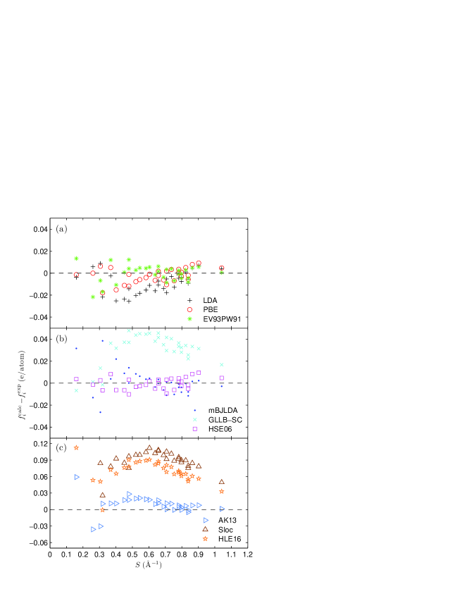
Figure 4: Difference between the experimental and calculated form factors of Si in Table S3 plotted as a function of $S=\sin\left(\theta\right)/\lambda$. The errors with Sloc for the 1st (111) and 2nd (220) form factors are 0.22 and 0.13 e/atom, respectively, and outside the range of the $y$-axis range. Note that the scale of the $y$-axis in panel (c) is different from the one in panels (a) and (b). The results for BJLDA and LB94 are omitted.

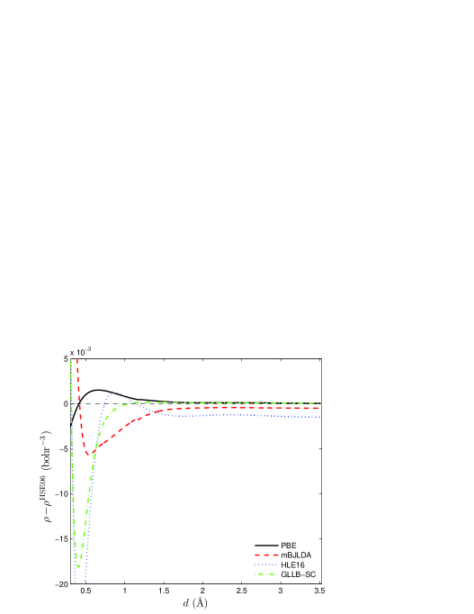
Figure 5: Difference between the electron density $\rho$ in Si obtained with various potentials and the one from HSE06 which is considered as the reference. The plot is along a path starting at a distance of $d=0.3$ Å from the atom at $\left(\frac{1}{8},\frac{1}{8},\frac{1}{8}\right)$ in the direction of the center of the unit cell which is at $d=3.527$ Å.

The last property that we want to consider in order to judge the quality of the xc potentials is the electron density of Si, for which X-ray structure factors have been experimentally measured for the reflections from (111) to (880) and the Si form factors derived from them.Saka and Kato (1986); Cumming and Hart (1988) The calculated values are given in Table S3 of the Supplemental MaterialSM_ and the deviations with experiment are shown graphically in Fig. 4. As done in previous works (see, e.g., Refs. Lu et al., 1993; Zuo et al., 1997) the agreement with experiment is quantified in terms of $R$-factor and goodness-of-fit (GoF) (defined in the caption of Table 6). The results in Table 6 show that the lowest errors, $R=0.10$% and $\text{GoF}=5.5$, are obtained with the hybrid functional HSE06. The best nonhybrid methods are PBE, EV93PW91, and BJLDA which lead to values for $R$ and GoF that are slightly larger than with HSE06. Next come LDA and mBJLDA which lead to very similar values for $R$ and GoF, that are roughly two (for $R$) or three (for GoF) times larger than with PBE and EV93PW91. The most inaccurate electron densities are obtained with Sloc and HLE16, since the values for $R$ and GoF are one and two orders of magnitude larger, respectively. The errors obtained with GLLB-SC are also significant since $R=0.75$% and $\text{GoF}=240$.

It is also instructive to look at the form factors individually in order to have a clue about which part of the electron density (shown in Fig. 5) is described (in)accurately by a given potential. The bonding/valence region is revealed by the low-order form factors (very roughly, corresponding to $S\lesssim 0.3$ Å^-1 in Fig. 4), while the high-order ones correspond to the high density of the semicore and core electrons that are localized around the nucleus. As discussed in Ref. Zuo et al., 1997, the use of EV93 for exchange (that was combined with LDA for correlation in that work) improves the description of the core density (in particular of the $2s$- and $2p$-electron subshells), but deteriorates the accuracy of the bonding region compared to LDA and the GGA PW91Perdew et al. (1992) (very similar to PBE). This is confirmed in Fig. 4(a), where we can see that the deviations from experiment with EV93PW91 are larger for the first five form factors, but smaller on average for the higher ones compared to LDA and PBE. An explanation for this may be that the exchange EV93 functional was fitted to the EXX-OEP in atoms, which is possibly more accurate than standard LDA/PBE for core electrons.

The mBJLDA potential [see Figs. 4(b) and 5] is quite inaccurate for the bonding region, since for the first few low-order form factors the errors are quite large, and slightly larger than with EV93PW91. However, for the (semi)core density, mBJLDA is of similar accuracy as PBE and EV93PW91, and therefore quite accurate. The GLLB-SC potential shows the opposite trend compared to mBJLDA: accurate bonding/valence electron density (small errors for the first four form factors) and very inaccurate core density (large errors for all other form factors). The HSE06 functionals leads to errors that are small for all form factors. Figure 4(c) shows that the Sloc and HLE16 potentials lead to extremely inaccurate electron density in general. The errors $f_{i}^{\text{calc}}-f_{i}^{\text{exp}}$ are in the range 0.05-0.12 e/atom for most form factors, while the errors with LDA, PBE, and EV93PW91 are all below 0.02 e/atom. Figure 5 shows indeed that the error in the electron density (HSE06 is chosen as the reference) with HLE16 is much larger than with PBE in the semicore and valence regions. Concerning the AK13 potential, the errors are very large for the first three form factors (i.e., the valence $3s$ and $3p$ electrons), but more or less of the same magnitude as LDA (but with opposite sign) for the others, which represent the core density.

The main conclusion of this section is that among the semilocal methods, PBE is the most accurate for the electron density of Si. The other methods are less accurate for the core and/or valence parts of the electron density. The GLLB-SC potential seems to be as accurate as PBE for the valence/bonding density, which is consistent with the observations made in Sec. III.3 for the EFG that is determined mainly by the valence electron density. The mBJLDA potential describes quite well the core density, but not the valence density. Overall, the best performance is obtained with the hybrid HSE06.

III.5 Further discussion

III.5.1 Visualization of the xc potentials

The results presented above should provide some guidance when choosing (within the KS method) an exchange-correlation potential that is adequate for the problem at hand. However, it has also been clearly shown that none of the tested potentials leads to sufficiently accurate results in all circumstances, which is hardly surprising with semilocal and hybrid methods. The search for a fast semilocal multiplicative xc potential which is more universally accurate than those presented above is certainly not an easy task. However, in this respect it may be helpful to try to understand what is going on in terms of the shape of the potentials considered in this work.

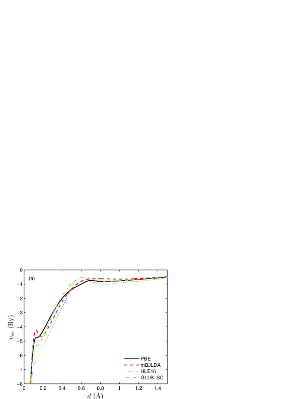
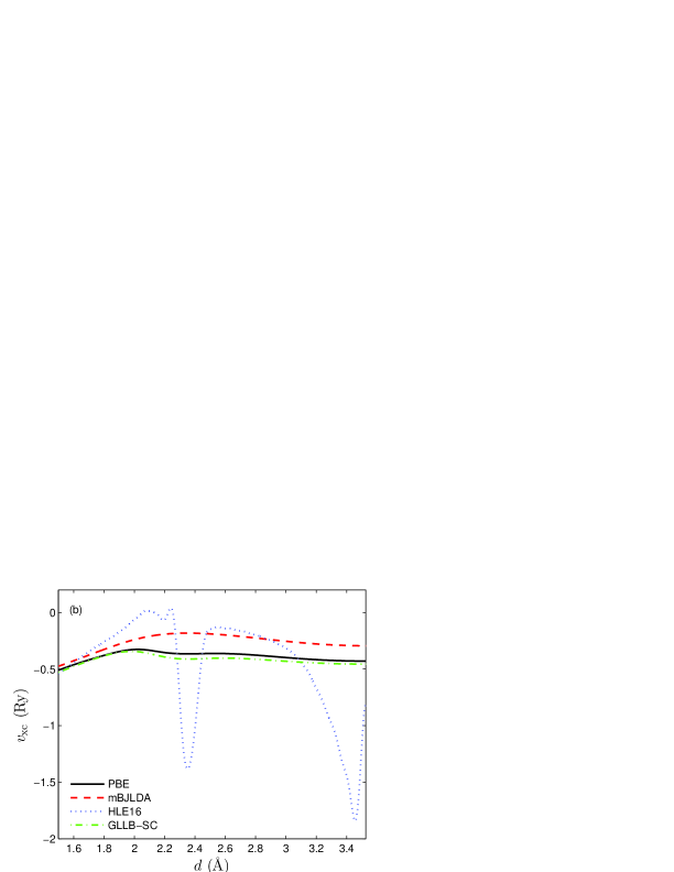
Figure 6: Potentials $v_{\text{xc}}$ in Si plotted from the atom at $(\frac{1}{8},\frac{1}{8},\frac{1}{8})$ ($d=0$) to the center of the unit cell which is at $d=3.527$ Å.

In previous works, Städele et al. (1997, 1999); Aulbur et al. (2000); Qteish et al. (2006); Tran et al. (2007); Betzinger et al. (2011); Koller et al. (2011); Tran et al. (2015a, b, 2016) trends in the results could be understood by comparing the shape of the potentials. Basically, the magnitude of the band gap and magnetic moment are directly related to the inhomogeneities in the potential, and it was observed and rationalized that more pronounced inhomogeneities favor larger values of the band gap and magnetic moment. In order to understand some of the results discussed in the previous sections, two cases are now studied in more detail.

In Sec. III.4, we showed that some of the potentials lead to very inaccurate electron density in Si. For instance, the densities obtained with Sloc, HLE16, and GLLB-SC differ quite significantly from the reference HSE06 density in the region close to the nucleus ($d\lesssim 0.7$ Å in Fig. 5). Taking a look at the potentials should help us to understand the reason for this, and actually Fig. 6(a) shows that from $d=0.1$ to 0.7 Å the magnitudes of the HLE16 and GLLB-SC potentials (Sloc is not shown but similar) vary faster than for PBE and mBJLDA, which are much more accurate for the (semi)core density. It is this (too) fast variation in $v_{\text{xc}}$ which leads to inaccurate density in the (semi)core region.

In our previous works,Tran et al. (2015a); Tran and Blaha (2017) we showed that the nonstandard GGA potentials EV93PW91, AK13, and HLE16 show large oscillations in the middle of the interstitial region [visible for $d$ larger than 1.5 Å in Si, see Fig. 6(b)], which should mainly be a consequence of their strong dependence on the second derivative of $\rho$. This is not the case for the BJ-type potentials and EXX-OEP which were shown to be rather flat (as LDA and PBE) in the interstitial. The RPA-OEP also seems to be smooth according to Ref. Klimeš and Kresse, 2014. Since the GLLB-SC potential depends on the second derivative of $\rho$ only via the correlation potential $v_{\text{c}}^{\text{PBEsol}}$, i.e. weakly, it is also smooth in the interstitial and very close to PBE (and LDA) as shown in Fig. 6(b).

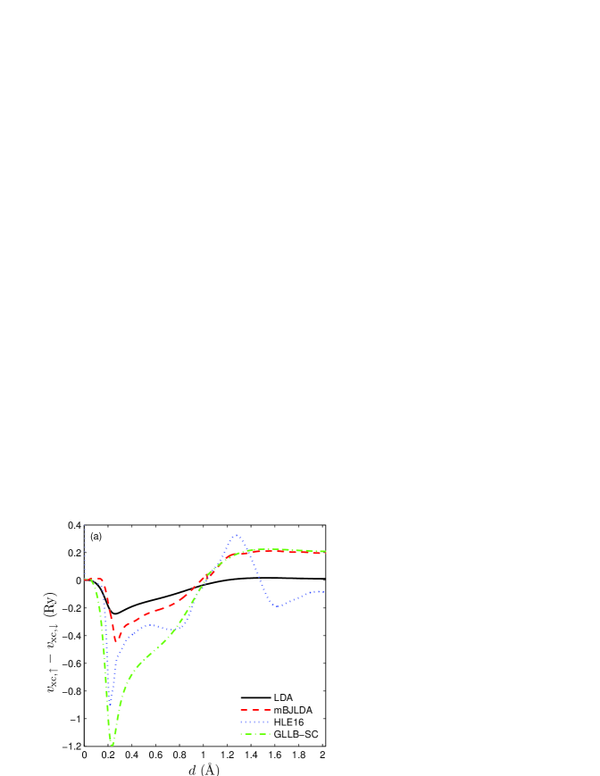
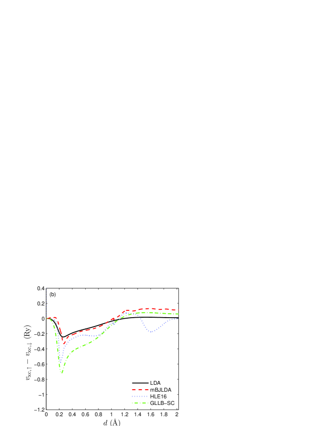
Figure 7: $v_{\text{xc},\uparrow}-v_{\text{xc},\downarrow}$ in Fe plotted from the atom at (0,0,0) of the body-centered cubic cell to $\left(\frac{1}{2},\frac{1}{2},0\right)$ (middle of a face of the cell). (a) shows the potentials of the self-consistent calculations, while (b) shows the potentials calculated non-self-consistently using $\rho_{\sigma}$, $t_{\sigma}$, and $\psi_{i\sigma}$ from the LDA calculation.

One of the problems of GLLB-SC is to overestimate the exchange splitting in metals and, therefore, the magnetic moment in Fe, Co, and Ni. Figure 7(a) shows the difference $v_{\text{xc},\uparrow}-v_{\text{xc},\downarrow}$ between the self-consistent spin-up and spin-down xc potentials in Fe, where we can see that it is the largest for GLLB-SC. The large exchange splitting observed in Fig. 3 for HLE16 can also be understood from the large magnitude of $v_{\text{xc},\uparrow}-v_{\text{xc},\downarrow}$. Note that for $d\gtrsim 1$ Å, the mBJLDA and GLLB-SC potentials coincide very closely. Besides this, we can also see that $v_{\text{xc},\uparrow}-v_{\text{xc},\downarrow}$ is negative until $d\sim 1$ Å and then positive in some cases. The negative region is where the $3d$ electrons, which are the main contributors to the magnetic moment, are located, while the positive region is the interstitial where the $s$ and $p$ electrons, which also contribute to the magnetic moment but with opposite sign and a much smaller magnitude,Moon (1964); Mook (1966) are found. Just to give some examples, the $d$ ($d$ inside the atomic sphere) and $sp$ ($sp$ inside the atomic sphere and total from interstitial) contributions to the spin magnetic moment of Fe are 2.21 and 0.00 $\mu_{\text{B}}$ with LDA, 2.76 and -0.25 $\mu_{\text{B}}$ with mBJLDA, and 3.41 and -0.34 $\mu_{\text{B}}$ with GLLB-SC. Figure 7(b) also shows $v_{\text{xc},\uparrow}-v_{\text{xc},\downarrow}$, but this time evaluated non-self-consistently with the LDA density, orbitals, etc., where we can see that the magnitude is much smaller, indicating that the exchange splitting is strongly enhanced by the self-consistent field procedure.

III.5.2 Variants of GLLB-SC: Attempts of improvement

The results of the present and previous works Kuisma et al. (2010); Castelli et al. (2012); Yan et al. (2012); Hüser et al. (2013); Miró et al. (2014); Pilania et al. (2016); Kim et al. (2016); Pandey et al. (2017) have shown that the GLLB-SC potential is much more reliable for band gap calculation than all LDA and GGA methods that have been considered so far for comparison, and of quite similar accuracy as mBJLDA, the hybrids, and $GW$. Nevertheless, among the few problems of GLLB-SC that were pointed out, the most important are (1) a clear underestimation of most band gaps smaller than $\sim 1$ eV, (2) some unpredictable behavior for strongly correlated systems (for which mBJLDA is much more reliable), and (3) a very large overestimation of the magnetic moment of metals.

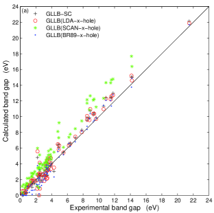
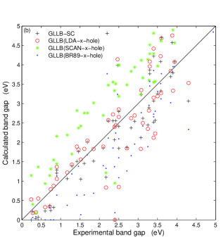
Figure 8: Calculated versus experimental fundamental band gaps for the set of 76 solids. The calculated values were obtained with GLLB-SC and various variants which differ in the exchange hole term. The lower panel is a zoom of the upper panel focusing on band gaps smaller than 5 eV.

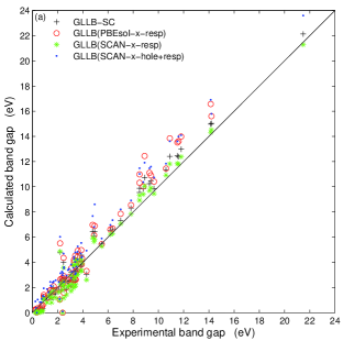
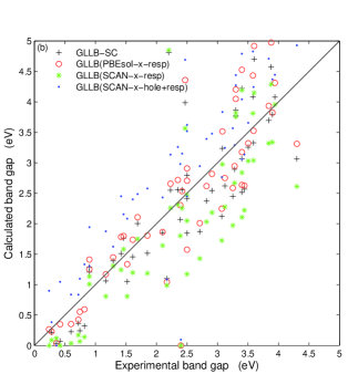
Figure 9: Calculated versus experimental fundamental band gaps for the set of 76 solids. The calculated values were obtained with GLLB-SC and various variants which differ in the exchange response term or in both the exchange hole and response terms. The lower panel is a zoom of the upper panel focusing on band gaps smaller than 5 eV.

Table 7: Summary statistics for the error in the calculated band gaps in Table S4 of the Supplemental MaterialSM_ for the set of 76 solids obtained with GLLB-SC and various variants which differ either in the exchange hole term, in the exchange response term, or both. The calculations were done at the experimental geometry specified in Table S1 of the Supplemental Material.SM_

	GLLB
	SC	LDA-x-hole	SCAN-x-hole	BR89-x-hole	PBEsol-x-resp	SCAN-x-resp	SCAN-x-hole+resp
ME (eV)	0.20	0.23	1.41	-0.24	0.55	-0.13	1.01
MAE (eV)	0.64	0.65	1.48	0.60	0.89	0.58	1.14
STDE (eV)	0.81	0.88	1.13	0.73	1.15	0.76	1.05
MRE (%)	-4	4	46	-21	6	-15	31
MARE (%)	24	22	50	28	24	26	38
STDRE (%)	34	35	56	36	33	36	47

As said in the introduction, the idea behind the construction of the GLLB(-SC) potential is very interesting, but also very promising since it allows for a proper calculation of the band gap at a computational cost that is similar to semilocal methods. Therefore, it is certainly worth to explore further the GLLB idea, and the important question is to which extent is it possible to improve upon GLLB-SC without deteriorating the results which are already good. To try to answer this question we have considered several variants of Eq. (5), and one of the most obvious modifications consists of choosing an alternative to $2\varepsilon_{\text{x},\sigma}^{\text{PBEsol}}$ for the exchange hole term $v_{\text{x,hole},\sigma}$, while keeping the second and third terms the same as in GLLB-SC. Among the numerous choices that we have tried for $v_{\text{x,hole},\sigma}$, three of them will be discussed, namely, $2\varepsilon_{\text{x},\sigma}^{\text{LDA}}$, $2\varepsilon_{\text{x},\sigma}^{\text{SCAN}}$, and $v_{\text{x},\sigma}^{\text{BR89}}$. The latter two are MGGA since $\varepsilon_{\text{x},\sigma}^{\text{SCAN}}$ is $t_{\sigma}$-dependent,Sun et al. (2015a) while $v_{\text{x},\sigma}^{\text{BR89}}$ is $t_{\sigma}$- and $\nabla^{2}\rho_{\sigma}$-dependent.Becke and Roussel (1989) BR89 was constructed to be similar to the Slater potentialBecke and Roussel (1989); Tran et al. (2015b) and is the hole term in the BJ potential.Becke and Johnson (2006) The results for the band gap can be found in Table S4 of the Supplemental MaterialSM_ and are shown in Fig. 8, while the average errors are in Table 7. Compared to the original version of the potential, the results obtained with GLLB(LDA-x-hole) and GLLB(BR89-x-hole) are rather similar in terms of MA(R)E and STD(R)E. However, GLLB(BR89-x-hole) leads to negative M(R)E, which is due to a clear underestimation of band gaps smaller than 4 eV [see Fig. 8(b)], and actually the band gap is zero for five solids (Ge, GaSb, InAs, InSb, and VO₂), while this was the case for only two solids with GLLB-SC. The opposite trend is observed with GLLB(LDA-x-hole), which is more accurate than GLLB-SC for the band gaps smaller than $\sim 1$ eV, such that only one system (FeO) is described as metallic. On the other hand, the band gaps in the range 2-5 eV are more underestimated with GLLB(LDA-x-hole) than with GLLB-SC. The band gaps obtained with GLLB(SCAN-x-hole) are too large with respect to experiment and overall the results are very inaccurate since the MAE and MARE are 1.48 eV and 50%, respectively.

Thus, replacing PBEsol by something else for the exchange hole term does not really help in improving the results overall, and the same conclusion can be drawn with the other choices for $v_{\text{x,hole},\sigma}$ that we have tested (results not shown), namely, $2\varepsilon_{\text{x},\sigma}$ of the exchange functionals EV93,Engel and Vosko (1993) revTPSS,Perdew et al. (2009) MVS,Sun et al. (2015b) and TM,Tao and Mo (2016) with the latter three being MGGA. The general observation is that a clear improvement for a group of band gaps that are, e.g., underestimated with GLLB-SC is necessarily accompanied by a clear deterioration for another group. Also, the case of the iron oxides FeO and Fe₂O₃ is particularly problematic. While GLLB-SC leads to no band gap in FeO (experiment is 2.4 eV) and strongly overestimates the value for Fe₂O₃ (4.81 eV versus 2.2 eV for experiment), GLLB-SC(SCAN-x-hole) improves the result for FeO (0.95 eV), but overestimates even more than GLLB-SC for Fe₂O₃ (5.99 eV).

The other type of variants of Eq. (5) that we have considered consists of an exchange response term that is multiplied by a function $F_{\sigma}$:

$$F_{\sigma}(\bm{r})K_{\text{x}}^{\text{LDA}}\sum_{i=1}^{N_{\sigma}}\sqrt{\epsilon_{\text{H}}-\epsilon_{i\sigma}}\frac{\left|\psi_{i\sigma}(\bm{r})\right|^{2}}{\rho_{\sigma}(\bm{r})}$$ (7)

and similarly in Eq. (6) for the associated derivative discontinuity. In order to be reasonable from the formal point of view, $F_{\sigma}$ should satisfy two constraints. The first one is $F_{\sigma}=1$ for a constant $\rho_{\sigma}$ such that the potential recovers LDA as GLLB-SC does. The second constraint requires $F_{\sigma}$ to be constructed such that the scaling property of the exchange potentialOu-Yang and Levy (1990) [$v_{\text{x}}([\rho_{\lambda}];\bm{r})=\lambda v_{\text{x}}([\rho];\lambda\bm{r})$, where $\rho_{\lambda}(\bm{r})=\lambda^{3}\rho(\lambda\bm{r})$] is satisfied, which is the case if $F_{\sigma}$ depends only on the reduced density gradient $s_{\sigma}=\left|\nabla\rho_{\sigma}\right|/\left(2\left(6\pi^{2}\right)^{1/3}\rho_{\sigma}^{4/3}\right)$ for a GGA-type $F_{\sigma}$, and on quantities like $t_{\sigma}^{\text{W}}/t_{\sigma}$ or $t_{\sigma}/t_{\sigma}^{\text{TF}}$ for a $t_{\sigma}$-dependent MGGA-type $F_{\sigma}$ [$t_{\sigma}^{\text{W}}=\left|\nabla\rho_{\sigma}\right|^{2}/\left(8\rho_{\sigma}\right)$ and $t_{\sigma}^{\text{TF}}=\left(3/10\right)\left(6\pi^{2}\right)^{2/3}\rho_{\sigma}^{5/3}$ are the von Weizsäckervon Weizsäcker (1935) and Thomas-Fermi kinetic-energy densityThomas (1927); Fermi (1927)]. Thus, a possible choice for $F_{\sigma}$ in Eq. (7) would be to use (blindly) any of the GGA or MGGA exchange enhancement factors $F_{\text{x},\sigma}^{\text{(M)GGA}}=\varepsilon_{\text{x},\sigma}^{\text{(M)GGA}}/\varepsilon_{\text{x},\sigma}^{\text{LDA}}$ that are available in the literature. Such a choice could seem quite empirical and not justified, but it should just be considered as the first attempt to improve the results by making Eq. (7) $\nabla\rho_{\sigma}$- or $t_{\sigma}$-dependent.

The results for the band gap obtained with two different exchange enhancement factors for $F_{\sigma}$ in Eq. (7), namely $F_{\text{x},\sigma}^{\text{PBEsol}}$ and $F_{\text{x},\sigma}^{\text{SCAN}}$ (as in GLLB-SC, we keep PBEsol for $v_{\text{x,hole},\sigma}$ and $v_{\text{c},\sigma}$), are shown in Fig. 9 and Tables S4 and 7. The results are rather disappointing and the trends are similar to those discussed above when different exchange hole terms were considered. Compared to GLLB-SC, GLLB(PBEsol-x-resp) and GLLB(SCAN-x-resp) lead to band gaps which are larger and smaller, respectively. Since the direction of change in the band gap is the same in basically all cases, an improvement for the underestimated band gaps (e.g., the small ones) is associated with an overestimation for most other solids, or vice versa.

Figure 9 and Tables S4 and 7 also show the results obtained with GLLB(SCAN-x-hole+resp) which consists of using SCAN exchange for the hole and response terms simultaneously. The accuracy of GLLB(SCAN-x-hole+resp) is in between those of GLLB(SCAN-x-hole) and GLLB(SCAN-x-resp), and overall rather low since the MAE and MARE are quite large (1.14 eV and 38%). Not shown, the results obtained with the MGGA exchange MVSSun et al. (2015b) or TMTao and Mo (2016) instead of SCAN for the hole and response terms indicate that TM leads to reduced errors (but still larger than GLLB-SC), while with MVS the errors are similar to SCAN.

The other possibilities for $F_{\sigma}$ in Eq. (7) that we have tried are simple MGGA functions $F_{\sigma}=\left(t_{\sigma}/t_{\sigma}^{\text{TF}}\right)^{p}$ or $F_{\sigma}=\left(\left(t_{\sigma}-t_{\sigma}^{\text{W}}\right)/t_{\sigma}^{\text{TF}}\right)^{p}$, which are somehow similar to the response terms $v_{\text{x,resp},\sigma}^{\text{BJ}}\propto\sqrt{t_{\sigma}/\rho_{\sigma}}$ and $v_{\text{x,resp},\sigma}^{\text{BJUC}}\propto\sqrt{\left(t_{\sigma}-t_{\sigma}^{\text{W}}\right)/\rho_{\sigma}}$ of the BJ potentialBecke and Johnson (2006) and its gauge-invariant version (universal correction),Räsänen et al. (2010) respectively. Using such functions should be promising since this is a way to apply the GLLB idea to a potential whose response term is somehow similar to the BJ potential. However, the results that we have obtained so far with such functions $F$ are not very encouraging and are not worth to be discussed in detail. Nevertheless, we believe that the search for such simple functions depending on the kinetic-energy density that could lead to interesting results is worth to be pursued.

The last variant of GLLB-type potential that we have considered is given by

$$v_{\text{xc},\sigma}^{\text{GLLB2-SC}}(\bm{r}) = 2\varepsilon_{\text{xc},\sigma}^{\text{PBEsol}}(\bm{r})+F_{\text{xc},\sigma}^{\text{PBEsol}}(\bm{r})$$ (8)

$$\times K_{\text{x}}^{\text{LDA}}\sum_{i=1}^{N_{\sigma}}\sqrt{\epsilon_{\text{H}}-\epsilon_{i\sigma}}\frac{\left|\psi_{i\sigma}(\bm{r})\right|^{2}}{\rho_{\sigma}(\bm{r})},$$

where $F_{\text{xc},\sigma}^{\text{PBEsol}}=\varepsilon_{\text{xc},\sigma}^{\text{PBEsol}}/\varepsilon_{\text{x},\sigma}^{\text{LDA}}$ is the total PBEsol enhancement factor.Perdew et al. (2008) Compared to GLLB-SC [Eq. (5)], correlation is now treated the same way as exchange and, therefore, also contributes to the derivative discontinuity. Equation (8) should be considered as a simple, but still rather meaningful way to extend GLLB-SC to correlation. As discussed in Sec. III.1, GLLB2-SC leads to a xc discontinuity that agrees very well with the RPA-OEP value for simple solids. However, the calculated band gaps with GLLB2-SC are quite inaccurate such that the ME and MAE are 1.35 and 1.47 eV, respectively. A large overestimation is obtained for most solids, except for those with a band gap smaller than 1 eV and a few others like FeO for which the band gap is still zero. Thus, for band gap calculation GLLB2-SC is of no interest and does not solve the problems found with GLLB-SC. Replacing PBEsol by SCAN in Eq. (8) also does not lead to any interesting improvement in the band gaps.

In this section, numerous attempts to improve upon the original GLLB-SC method have been presented. However, the results are rather disappointing since none of the variants of GLLB-SC that we have tested could really solve the problems of GLLB-SC for the band gap. We also mention that it has not been possible to really reduce the large overestimation of the magnetic moment in ferromagnetic metals compared to GLLB-SC. The fact that absolutely all variants of the GLLB-SC potential mentioned above lead to such large overestimation of $\mu_{S}$ strongly suggests that this problem is due to the dependency on the orbital energies $\epsilon_{i}$ of the second term of Eq. (5) which makes $v_{\text{xc},\uparrow}^{\text{GLLB-SC}}-v_{\text{xc},\downarrow}^{\text{GLLB-SC}}$ too large when $\epsilon_{i\uparrow}\neq\epsilon_{i\downarrow}$. Without entering into details, reducing the magnitude of the second term in Eq. (5) (instead of increasing it as done above) with various schemes did not lead to satisfying results. Work is under way in order to find such a scheme that reduces the exchange splitting of metals without deteriorating too much the results for other systems.

As shown above, the mBJLDA potential leads to much more balanced results for the magnetic moment (very accurate for strongly correlated solids and moderately overestimated for metals). This is mainly due to the use of the average of $\nabla\rho/\rho$ in the unit cell, which is larger in the transition-metal oxides (1.9-1.95 bohr^-1/2) than in the ferromagnetic metals (1.4-1.5 bohr^-1/2) and therefore provides a way to make the difference between the two classes of solids (see Ref. Koller et al., 2011 for related discussions). Thus, the use of the average of $\nabla\rho/\rho$ or another similar quantity in a GLLB-type potential should also be considered in future works.

IV Summary and conclusion

In this work, the GLLB-SC potential has been tested and compared to other methods for the description of the electronic and magnetic properties of solids, as well as properties directly related to the electron density. Concerning the band gap, GLLB-SC is, as expected, much more accurate than the LDA and GGA methods and of similar accuracy as hybrid functionals. However, GLLB-SC is on average not as accurate as mBJLDA, and the two main problems are (1) a clear underestimation of band gaps smaller than 1 eV and (2) very large variations in the error for strongly correlated solids. mBJLDA is overall less prone to large errors than GLLB-SC, in particular for the strongly correlated solids. However, mBJLDA clearly underestimates the band gap of Cu¹⁺ compounds like Cu₂O.

The magnetic moment in antiferromagnetic insulators is accurately described by GLLB-SC, mBJLDA, and the hybrid functional HSE06, while for the ferromagnetic metals GLLB-SC and HSE06 lead to very large overestimations of the magnetic moment. The mBJLDA potential also overestimates the magnetic moment in the metals, but to a much lesser extent. Concerning the EFG, it has been shown that GLLB-SC is the method leading to the best agreement with experiment, meaning that the valence electron density should be described accurately by GLLB-SC. This is, however, not the case with mBJLDA which is not recommended for EFG calculations.

Focusing on the band gap, the goal was then to improve the results with respect to GLLB-SC by modifying either the hole term or the response term (or both) in the potential. However, our numerous attempts have remained fruitless, and actually it was not possible to improve significantly the results for a group of solids (e.g., those with a small band gap) without significantly worsening the results for other compounds. This is rather disappointing, in particular since more was expected by bringing in a dependency on the kinetic-energy density into a GLLB-type potential.

Nevertheless, a multiplicative xc potential that has the same features as GLLB-SC, namely, to be computationally fast and leads to a nonzero derivative discontinuity, is ideal from the formal and practical points of view, similarly as the nonmultiplicative potentials that are functional derivatives of MGGA functionals. Peverati and Truhlar (2012); Yang et al. (2016) Therefore, it is certainly worth to pursue the development of such potentials, possibly by trying to incorporate more features of other successful semilocal potentials like mBJLDA or AK13, or by learning more from very accurate ab initio potentials. Klimeš and Kresse (2014); Grabowski et al. (2014); Ospadov et al. (2017) In this respect, we should remind that the mBJLDA potential uses an ingredient, the average of $\nabla\rho/\rho$ in the unit cell that has not been used in other potentials except hybrid functionals. Bylander and Kleinman (1990); Seidl et al. (1996); Marques et al. (2011) Alternatively, the dielectric function could be used, Marques et al. (2011); Koller et al. (2013); Skone et al. (2014); Shimazaki and Nakajima (2015) however this requires the use of unoccupied orbitals. Also not yet explored, is the possibility to use the step structure of the BJ potential,Armiento et al. (2008) which in principle should lead to a derivative discontinuity (which is not the case with the AK13 potential as shown in Ref. Aschebrock et al., 2017b).