The one-dimensional asymmetric persistent random walk

Abstract

Persistent random walks are intermediate transport processes between a uniform rectilinear motion and a Brownian motion. They are formed by successive steps of random finite lengths and directions travelled at a fixed speed. The isotropic and symmetric one-dimensional persistent random walk is governed by the telegrapher’s equation, also called hyperbolic heat conduction equation. These equations have been designed to resolve the paradox of the infinite speed in the heat and diffusion equations. The finiteness of both the speed and the correlation length leads to several classes of random walks: Persistent random walk in one dimension can display anomalies that cannot arise for Brownian motion such as anisotropy and asymmetries. In this work we focus on the case where the mean free path is anisotropic, the only anomaly leading to a physics that is different from the telegrapher’s case. We derive exact expression of its Green’s function, for its scattering statistics and distribution of first-passage time at the origin. The phenomenology of the latter shows a transition for quantities like the escape probability and the residence time.

1 Introduction

Since it was introduced in Physics by Smoluchowski, Einstein and Langevin, Brownian motion has been studied and used in an ever growing range of purposes to describe randomness of various kinds. The probability distribution function of Brownian motion is the same as the Green’s function of the heat equation and the diffusion equation. However it was soon remarked that these equations are not compatible with causality, because they do not bound the instantaneous speed of motion. Brownian motion is therefore only a limit of a more complex motion, observed at large time and length scales. At the atomic scale, the movement of the walkers is not Brownian anymore, it is a sequence of rectilinear motions interspersed by collisions. Such a movement is a random walk with steps of finite lengths and finite time steps. Calling $\ell$ the average step length — the mean free path — and $\tau$ the average time between two collisions, the speed is $c=\ell/\tau$. Brownian motion corresponds to the limit $\ell\to 0$ and $\tau\to 0$ when $\ell^{2}/\tau=D$ is kept constant. Under this limit, the speed $\ell/\tau$ must diverge.

It is widely known that the spatial probability distribution of presence of the Brownian motion is a Gaussian distribution. The Fokker-Planck equation of Brownian motion is the diffusion equation and is the same as the heat equation. Although these equations are used in many physical models, they do not fulfill the requirement of causality that is imposed to any physical equation. The absence of causality and the possible corrections to restore it in the heat equation have been discussed by Cattaneo [1] and Vernotte [2]. They independently proposed a microscopical theory yielding a supplementary term of second order time derivative in the equation. The obtained equation is the so-called telegrapher’s equation, first derived by Thomson when he was studying the electric transport in the first transatlantic cable [3]. The theory of heat waves has widely developped. For a complete review until 1989, refer to the exhaustive work of Joseph and Preziosi [4]. Other works on the diffusion equation, that suggested to add an inertial term, obtained the same equation [5, 6].

In 1951, Goldstein showed that the telegrapher’s equation is the Fokker-Planck equation of a persistent random walk with a fixed time step [7]. Persistent random walks were introduced by Fürth [8] and Taylor [9]. In higher dimensions, another approach was proposed by Domb and Fisher [10]. In 1965, Montroll and Weiss generalized the random walks to a continuous time process, with random time steps [11]. Masoliver, Lindenberg and Weiss introduced the persistent random walk with continuous time steps [12].

The telegrapher’s equation appears to be the one-dimensional version of the radiative transfer equation. In scattering medium, waves propagate according to the radiative transfer equation [13]. In this equation the direction of the partial waves scattered by an impurity is correlated to the direction of the incoming wave. Consequently, the direction of propagation has a correlation length called the persistence length or the transport mean free path $\ell^{\star}$. In one dimension, this length can be different for walkers moving to the right (direction denoted as $\oplus$) and walkers moving to the left ($\ominus$). Such an anisotropy can arise from the scattering mechanism itself, from internal mechanisms or from external forces. It corresponds to the case where the rate of change from $\oplus$ into $\ominus$ is different from the rate of change from $\ominus$ into $\oplus$. Asymmetric persistent random walks have been used to study the instability dynamics of microtubules [14]. In microtubule, the $\oplus$ and $\ominus$ directions correspond to growth or shrinkage of the one end of the microtubule. As these are different chemical processes, their characteristics speeds and persistence lengths are different. Persistent random walks have also been considered in the context of relativistic Brownian motion [15].

A random walker can reach, after some time, the boundary of its propagation domain, where it will be reflected or absorbed, for instance by a detection device. The location on the boundary and the time at which it is reached are relevant quantities to investigate the propagation properties. First passage problems are ubiquitous in physical sciences and have been widely studied [16, 17]. Their properties are mostly studied for Brownian motion in several situations in two and even in higher dimensions [18]. The statistics of the first passage times of the persistent random walk have been studied by Masoliver, Porrà and Weiss [19].

Most of the cited studies of the one-dimensional persistent random walk have been performed in the case where the mean free path is isotropic. In this article, we start by showing that mean free path anisotropy is actually the only candidate for new physics within all possible transport and scattering anomalies in one dimension. The next sections of this work are dedicated to the derivation and solution of the asymmetric equation. We show that the number of scattering events follows a distribution obtained using the same functions. In the last section, we study the first-passage time distribution at the origin and show that it posseses a very intuitive phenomenology and transitions around the symmetry point.

2 The asymmetric one-dimensional persistent random walks

In this section we discuss the properties of one-dimensional random walks and their asymmetries. The one-dimensional space is indexed by $x\in\mathbf{R}$, a real number. In one dimension only two directions of propagation are possible, $\oplus$ and $\ominus$, which makes one dimensional random walks particular.

We consider a random walker moving along a one dimensional space containing scatterers. The positions of the scatterers are not fixed, they uniformly distributed along space and time. (This has the advantage to yield a time-invariant model.) The walker moves at a constant speed $c$ as long as it does not encounter any scatterer. When it meets a scatterer, it has a certain probability to change its directions. If it does not so, there is no observable sign that a scatterer was actually met. Contrary to the Brownian walker, the persistent walker has a definite velocity at almost all times. We can therefore count the time it spends moving in the $\oplus$ direction during the movement. We will denote this time by $t^{+}$. Similarly, the time spent moving in the $\ominus$ direction is denoted by $t^{-}$. The total time of displacement is of course $t=t^{+}+t^{-}$. If the displacement during this time is $x$, we have $x=c(t^{+}-t^{-})$, therefore we easily obtain $t^{\pm}=\frac{1}{2}(t\pm x/c)$.

Scattering anisotropy

In most of the studies of the persistent random walk, scattering is considered as instantaneous, isotropic and non-absorbing. We denote $p_{\text{back}}$ the probability that the walker changes its direction after a scattering event. The walker moves into one direction along an average distance of $\ell^{\star}=\ell/p_{\text{back}}$ (Note that if $p_{\text{back}}=0$, there is no scattering and the motion is rectilinear and uniform.) The length $\ell^{\star}$ is called the transport mean free path. In one dimension all anisotropic persistent random walks sharing the same transport mean free path are fully equivalent. The most studied case is the isotropic scattering case where $p_{\text{back}}=1/2$ and $\ell^{\star}=2\ell$ [20]. This case corresponds to the situation where the random walker is isotropically redirected as if it were a photon scattered in a cloud of point-like scatterers. Another interesting situation is the backward scattering case, where $p_{\text{back}}=1$, because the two mean free paths are equal. The backward scattering case is more intuitive and can be used to interpret more easily the distribution of probability of the position and direction of the random walker. In this work, we consider, without loss of generality, only the scattering mean free path $\ell^{\star}$ such that we will consider the situation $p_{\text{back}}=1$.

Transport asymmetries

We speak of asymmetry in the case where a physical constant for the walkers travelling in the $\oplus$ direction has a different value for the walkers travelling in the $\ominus$ direction. Since the physical constants describing the persistent random walk are the speed $c$, the transport mean free path $\ell^{\star}$ and the absorption $a$, we introduce the speeds $c^{+}$ and $c^{-}$, the transport mean free paths $\ell^{\star}_{+}$ and $\ell^{\star}_{-}$ and the absorptions $a^{+}$ and $a^{-}$, for the walkers moving in the directions $\oplus$ or $\ominus$ according to the sign.

A speed asymmetry can account for different polymerization and depolymerization rates in the case of microtubule dynamics [14]. The Galilean change of variable $x^{\prime}=x-vt$, with $v=({c^{+}-c^{-}})/2$, restores the speed symmetry in the translation frame $(x^{\prime},\,t)$ in which the speed is $c=(c^{+}+c^{-})/2$. An absorption asymmetry damps the whole solution by a factor $\exp(-a^{+}t^{+}-a^{-}t^{-})$ where $t^{\pm}$ is the time spent in the direction . Speed and absorption asymmetries can therefore be disposed of easily, all results obtained in the case where $c^{+}=c^{-}$ and $a^{+}=a^{-}=0$ can be extended to the general case by using a change of referential and by adding a damping factor.

We will focus our discussion on the mean free path asymmetry that yields non trivial features. We use the two transport mean free paths $\ell^{\star}_{+}$ and $\ell^{\star}_{-}$ to define the average transport mean free path $\ell^{\star}$, the attenuation rate $\mu$ and the the asymmetric wavenumber $\kappa$ as

$$\ell^{\star}=\sqrt{\ell^{\star}_{+}\ell^{\star}_{-}}\;,\;\;\mu=\frac{c}{2}\left(\frac{1}{\ell^{\star}_{+}}+\frac{1}{\ell^{\star}_{-}}\right)\;\text{and}\;\;\kappa=\frac{1}{2}\left(\frac{1}{\ell^{\star}_{-}}-\frac{1}{\ell^{\star}_{+}}\right).$$ (1)

They are related by $\mu^{2}/c^{2}-\kappa^{2}=1/(\ell^{\star})^{2}$. The sign of $\kappa$ characterizes the direction in which the transport mean free path is larger. If $\kappa>0$, we have $\ell^{\star}_{+}>\ell^{\star}_{-}$ such that the average distance travelled by the walker between two scattering events is larger in the $\oplus$ direction than in the $\ominus$. As a result, the mean position of the walker is drifting in the $\oplus$ direction.

In the next section, we derive the Fokker-Planck equation governing the probability density function of the position, that we call the asymmetrie telegrapher’s equation (ATE).

3 The asymmetric telegrapher’s equation

We denote by $p^{+}(x,\,t)$ and $p^{-}(x,\,t)$ the spatial probability densities at time $t$ of walkers moving in the direction $\oplus$ and $\ominus$ respectively. We have the following coupled master equations

$$\left\{\begin{array}[]{rcl}p^{+}(x,\,t+\Delta t)&=&\left(1-\frac{\Delta x}{\ell^{\star}_{+}}\right)p^{+}(x-\Delta x,\,t)+\frac{\Delta x}{\ell^{\star}_{-}}p^{-}(x+\Delta x,\,t),\\ p^{-}(x,\,t+\Delta t)&=&\left(1-\frac{\Delta x}{\ell^{\star}_{-}}\right)p^{-}(x+\Delta x,\,t)+\frac{\Delta x}{\ell^{\star}_{+}}p^{+}(x-\Delta x,\,t).\end{array}\right.$$ (2)

Let us expand to the first order in $\Delta x$ and $\Delta t$, and use the relation $\Delta x=c\Delta t$. We obtain two coupled partial differential equations for the total probability density $p=p^{+}+p^{-}$ and the current density $j=c(p^{+}-p^{-})$:

$$\partial_{t}{p}=-\partial_{x}{j},\qquad\partial_{t}{j}=-c^{2}\partial_{x}{p}-2\mu j+2\kappa c^{2}\,p.$$ (3)

The first of these equations is the continuity equation that ensures the conservation of probability. In the case where there is absorption, this equation is no longer satisfied. Eliminating $j$ we find

$$\left(\partial^{2}_{x}{}-\frac{1}{c^{2}}\partial^{2}_{t}{}-2\kappa\partial_{x}{}-\frac{2\mu}{c^{2}}\partial_{t}{}\right)p=0.$$ (4)

Let us remark that in the symmetric case $\kappa=0$, if $\mu\to 0$ ($\ell^{\star}\to\infty$), we obtain a one-dimensional wave equation whereas if $c\to\infty$ while the value of $c^{2}/\mu$ is kept constant, one obtains a diffusion equation. The equation (4) is an interpolation between these two equations. In the “wave” limit, disorder is lost and in the diffusive limit, causality is lost. In the symmetric case $\kappa=0$, the equation (4) is called the telegrapher’s equation. Observe that, thanks to the continuity equation, $j$ is also solution of this equation (with different initial conditions) and consequently so are $p^{+}$ and $p^{-}$.

For convenience, we use the length and time units such that $\ell^{\star}=1$, $c=1$. The dimension of $p^{+}$, $p^{-}$ and $p$ is an inverse length $\left[\mathrm{L}^{-1}\right]$, the dimension of $j$ is an inverse time $\left[\mathrm{T}^{-1}\right]$. The symmetric case is retrieved using $\mu=1$, $\kappa=0$.

4 Solutions of the asymmetric telegrapher’s equation

4.1 General solutions

Let us solve the equation (4) using both the Fourier transform in space and the Laplace transform in time. We denote by $\hat{f}(x,\,s)$ the Laplace transform of $f(x,\,t)$ and by $\tilde{f}(k,\,t)$ its Fourier transform. The double transform is denoted by $\hat{\tilde{f}}(k,\,s)$. Equation (4) becomes

$$\hat{\tilde{f}}(k,\,s)=\frac{(s+2\mu)\tilde{f}(k,\,0)+\partial_{t}{\tilde{f}}(k,\,0)}{s^{2}+2\mu s+k^{2}-2\mathrm{i}k\kappa}$$ (5)

I introduce the elementary function $g_{1}$ defined by

$$\hat{\tilde{g}}_{1}(k,\,s)=\frac{1}{(s+\mu)^{2}+(k-\mathrm{i}\kappa)^{2}-1}.$$ (6)

The function $g_{1}$ is ubiquitous in the statistical theory of the persistent random walks. The equation (6) shows that it is a non-persistent multiple scattering Green’s function, but $g_{1}$ is not the Green’s function of the telegrapher’s equation (4). Performing the inverse Fourier transform we get

$$\hat{g}_{1}(x,\,s)=\frac{1}{2}\frac{\mathrm{e}^{\kappa x-|x|\sqrt{(s+\mu)^{2}-1}}}{\sqrt{(s+\mu)^{2}-1}}$$ (7)

and the inverse Laplace transform is found in Ref. [21, 29.3.93] for $\hat{g}_{1}(x,\,s-\mu)$, which provides $g_{1}(x,\,t)\mathrm{e}^{\mu t}$. We define more generally $g_{z}$ as

$$g_{z}(x,\,t)=z\frac{\mathrm{e}^{\kappa x-\mu t}}{2}I_{0}\left(z\sqrt{t^{2}-{x}^{2}}\right)\Theta(t-|x|)$$ (8)

and use $g_{1}$ in this section. The variable $z$ will be used in the next section. We also introduce the function $u_{z}$

$$u_{z}(x,\,t)=z\frac{\mathrm{e}^{\kappa x-\mu t}}{2}\frac{I_{1}\left(z\sqrt{t^{2}-{x}^{2}}\right)}{\sqrt{t^{2}-{x}^{2}}}\Theta(t-|x|)$$ (9)

that appears in many developped expressions. Both $g_{1}$ and $u_{1}$ have a probabilistic interpretation that we discuss in the Section 5. Some mathematical relations between $g_{z}$ and $u_{z}$ are given in the appendix.

The solution to (4) in the $(x,\,s)$ domain with the initial conditions $f(x,\,0)=v(x)$ and $\partial_{t}{f}(x,\,0)=w(x)$ is obtained by spatial convolution from the expression (5) as

$$\hat{\tilde{f}}(x,\,s)=(s+2\mu)\hat{g}_{1}(x,\,s)\underset{x}{\otimes}v(x)+\hat{g}_{1}(x,s)\underset{x}{\otimes}w(x).$$ (10)

In the time domain, using (B.7), it translates into

$$\partial_{t}{g_{1}}(x,\,t)\underset{x}{\otimes}v(x)+g_{1}(x,t)\underset{x}{\otimes}\left(2\mu v(x)+w(x)\right).$$ (11)

4.2 The Green’s function of the ATE in a infinite domain

We denote by $p(x,\,t\,|\,x_{0},\,t_{0})$ the solution of the ATE with the initial position in $x_{0}$ at $t=t_{0}$. The Green’s function of the ATE (4) is $p(x,\,t\,|\,0,\,0)$. If there is no ambiguity, we write it simply as $p(x,t)$. The direction of propagation comes as an extra argument in the variables or in the initial conditions. The Green’s function with imposed initial velocity has initial conditions $p(x,\,0\,|\,\mathchoice{\leavevmode\hbox to7.13pt{\vbox to7.13pt{\text{[drawing]}}}}{\leavevmode\hbox to7.13pt{\vbox to7.13pt{\text{[drawing]}}}}{\leavevmode\hbox to5.5pt{\vbox to5.5pt{\text{[drawing]}}}}{\leavevmode\hbox to3.1pt{\vbox to3.1pt{\text{[drawing]}}}})=\operatorname{\delta}(x)$ and $j(x,\,0\,|\,\mathchoice{\leavevmode\hbox to7.13pt{\vbox to7.13pt{\text{[drawing]}}}}{\leavevmode\hbox to7.13pt{\vbox to7.13pt{\text{[drawing]}}}}{\leavevmode\hbox to5.5pt{\vbox to5.5pt{\text{[drawing]}}}}{\leavevmode\hbox to3.1pt{\vbox to3.1pt{\text{[drawing]}}}})=\pm\operatorname{\delta}(x)$. To use these initial conditions in equation (11) we compute $\partial_{t}{p}(x,\,0\,|\,\mathchoice{\leavevmode\hbox to7.13pt{\vbox to7.13pt{\text{[drawing]}}}}{\leavevmode\hbox to7.13pt{\vbox to7.13pt{\text{[drawing]}}}}{\leavevmode\hbox to5.5pt{\vbox to5.5pt{\text{[drawing]}}}}{\leavevmode\hbox to3.1pt{\vbox to3.1pt{\text{[drawing]}}}})=-\partial_{x}{j}(x,\,0\,|\,\mathchoice{\leavevmode\hbox to7.13pt{\vbox to7.13pt{\text{[drawing]}}}}{\leavevmode\hbox to7.13pt{\vbox to7.13pt{\text{[drawing]}}}}{\leavevmode\hbox to5.5pt{\vbox to5.5pt{\text{[drawing]}}}}{\leavevmode\hbox to3.1pt{\vbox to3.1pt{\text{[drawing]}}}})=\mp\operatorname{\delta}(x)$ which immediately gives the solution expressed by means of $g_{1}$

$$p(x,t|\mathchoice{\leavevmode\hbox to7.13pt{\vbox to7.13pt{\text{[drawing]}}}}{\leavevmode\hbox to7.13pt{\vbox to7.13pt{\text{[drawing]}}}}{\leavevmode\hbox to5.5pt{\vbox to5.5pt{\text{[drawing]}}}}{\leavevmode\hbox to3.1pt{\vbox to3.1pt{\text{[drawing]}}}})=\partial_{t}{g_{1}}(x,t)+2\mu g_{1}(x,t)\mp\partial_{x}{g_{1}}(x,t).$$ (12)

Using the relations (B.7) and (B.8), we readily obtain the expression of $p$ as

$$p(x,\,t|\,\mathchoice{\leavevmode\hbox to7.13pt{\vbox to7.13pt{\text{[drawing]}}}}{\leavevmode\hbox to7.13pt{\vbox to7.13pt{\text{[drawing]}}}}{\leavevmode\hbox to5.5pt{\vbox to5.5pt{\text{[drawing]}}}}{\leavevmode\hbox to3.1pt{\vbox to3.1pt{\text{[drawing]}}}})=\frac{1}{\ell^{\star}_{\pm}}g_{1}(x,\,t)+(t\pm x)u_{1}(x,\,t)+{\operatorname{\delta}(t\mp x)\mathrm{e}^{-t/\ell^{\star}_{\pm}}}.$$ (13)

This result is made of three terms. The scattering contributions $g_{1}$ and $u_{1}$ contain a step function $\Theta$ that ensures causality. The term with a Dirac distribution $\operatorname{\delta}$ is the contribution of the walkers that have not been scattered at all. This solution was obtained in the symmetric case $\ell^{\star}_{+}=\ell^{\star}_{-}$ for the initial condition where half the walkers are $\oplus$ and half are $\ominus$ by Goldstein [7], Morse and Feschbach [22, p. 865] and Hemmer [23]. It was later interpreted as the solution of the symmetric radiative transfer in one dimension by Paasschens [24]. Proceeding with the same method, using $v(x)=\pm\operatorname{\delta}(x)$ and $w(x)=-\operatorname{\delta^{\prime}}(x)\mp 2\mu\operatorname{\delta}(x)+2\kappa\operatorname{\delta}(x)$ in (11), we find

$$j(x,\,t\,|\,\mathchoice{\leavevmode\hbox to7.13pt{\vbox to7.13pt{\text{[drawing]}}}}{\leavevmode\hbox to7.13pt{\vbox to7.13pt{\text{[drawing]}}}}{\leavevmode\hbox to5.5pt{\vbox to5.5pt{\text{[drawing]}}}}{\leavevmode\hbox to3.1pt{\vbox to3.1pt{\text{[drawing]}}}})=\pm\partial_{t}{g_{1}}(x,\,t)+2\kappa g_{1}(x,t)-\partial_{x}{g_{1}}(x,t),$$ (14)

or, in terms of $g$ and $u$

$$j(x,\,t\,|\,\mathchoice{\leavevmode\hbox to7.13pt{\vbox to7.13pt{\text{[drawing]}}}}{\leavevmode\hbox to7.13pt{\vbox to7.13pt{\text{[drawing]}}}}{\leavevmode\hbox to5.5pt{\vbox to5.5pt{\text{[drawing]}}}}{\leavevmode\hbox to3.1pt{\vbox to3.1pt{\text{[drawing]}}}})=\pm\left[-\frac{1}{\ell^{\star}_{\pm}}g_{1}(x,\,t)+(t\pm x)u_{1}(x,t)+{\operatorname{\delta}(t\mp x)\mathrm{e}^{-t/\ell^{\star}_{\pm}}}\right].$$ (15)

We observe that $j$ has the same terms as $p$ with different signs. This fact will find an explanation in the Section 5.

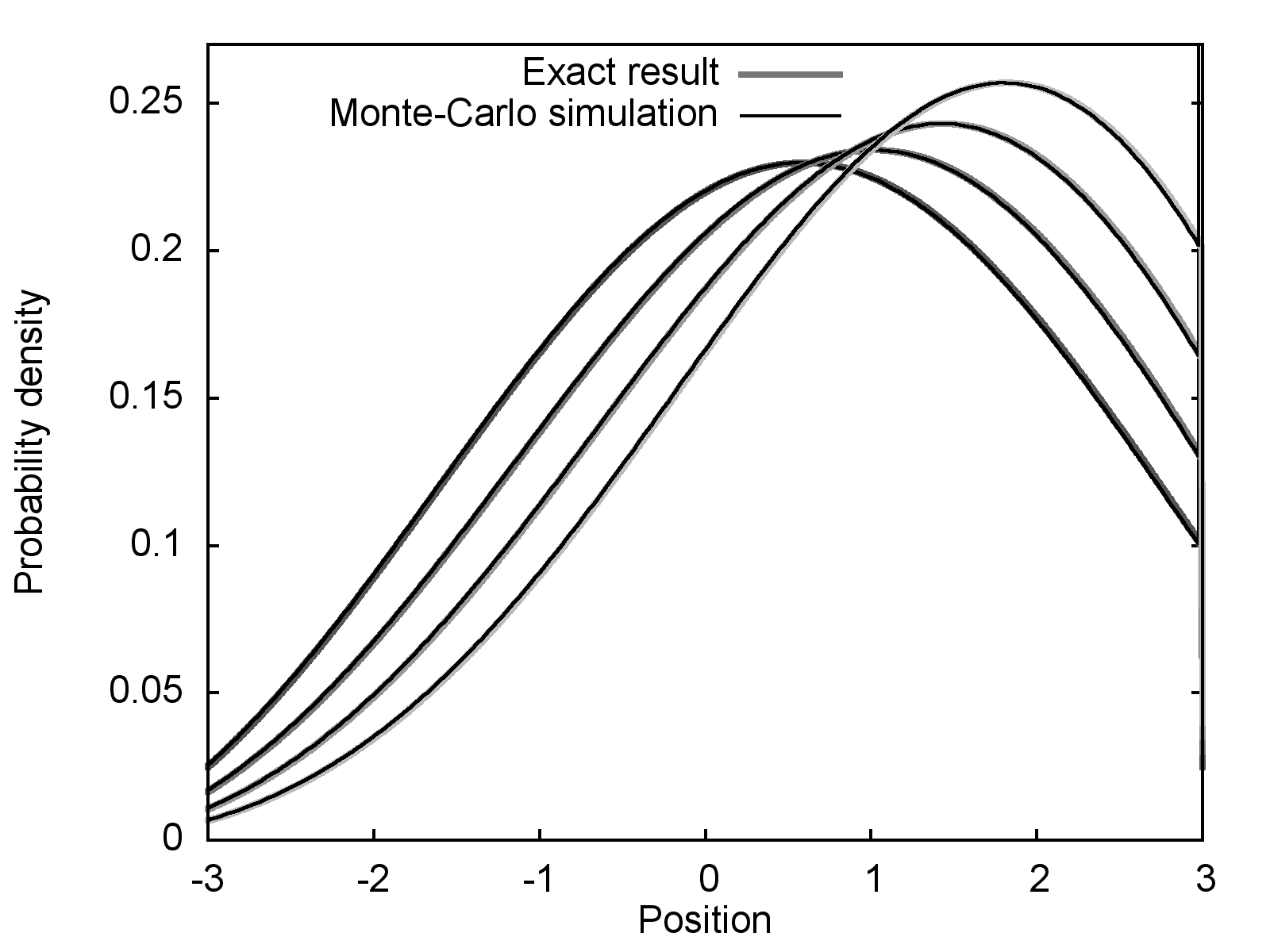
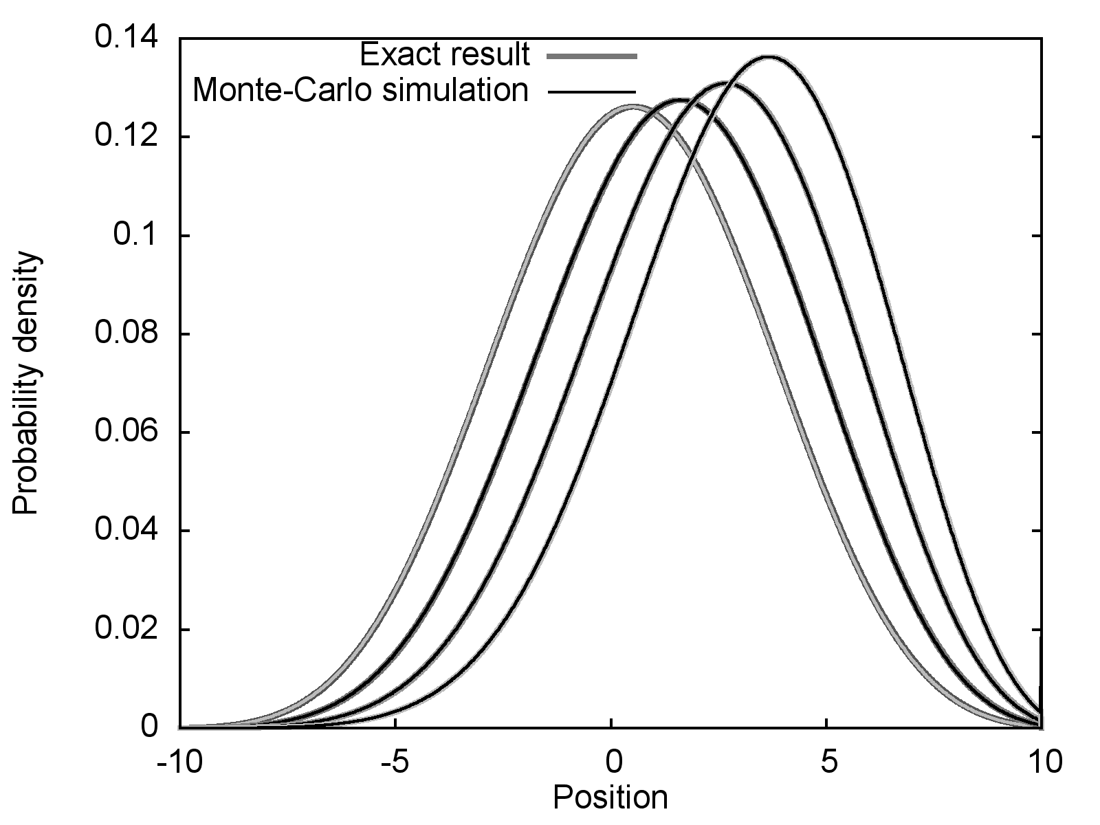
Figure 1: Spatial distribution of the persistent random walker after a time $t=3$ (Left) and $t=10$ (Right) for different values of the asymmetry parameter $\kappa$. The unbiased distribution ($\kappa=0$) reaches its maximum at $x=0$. The other distributions have been obtained for $\kappa=0.1$, $\kappa=0.2$ and $\kappa=0.3$. The exact result of Equation (13) is displayed with a thick line. The superimposed thin line has been obtained using a Monte-Carlo simulation of the persistent random walk. The random walk starts in the direction $\oplus$. Each step length is randomly generated using an exponential distribution $\mathrm{p}(x)=\ell^{-1}\mathrm{e}^{-x/\ell}$ where $\ell=\ell^{\star}_{+}$ or $\ell^{\star}_{-}$ according to the direction of propagation. After moving along one step, the direction is changed into its opposite (corresponding to the case $p_{\text{back}}=1$). The statistics have been performed using $10^{10}$ independent realizations of the random walk.

4.3 Direction of propagation

Let us consider the walkers starting in the $\oplus$ state and compute $p^{\pm}=(p\pm j)/2$ using the expressions (13) and (15). We obtain

$$p^{+}(x,\,t\,|\,\oplus) =(t+x)u_{1}(x,\,t)+{\operatorname{\delta}(t-x)\mathrm{e}^{-t/\ell^{\star}_{+}}} p^{-}(x,\,t\,|\,\oplus) =\frac{1}{\ell^{\star}_{+}}g_{1}(x,\,t).$$ and (16)

For the walkers starting in the $\ominus$ state, we find similar results

$$p^{-}(x,\,t\,|\,\ominus) =(t-x)u_{1}(x,\,t)+{\operatorname{\delta}(t+x)\mathrm{e}^{-t/\ell^{\star}_{-}}} p^{+}(x,\,t\,|\,\ominus) =\frac{1}{\ell^{\star}_{-}}g_{1}(x,\,t).$$ and (17)

Note that the above expressions are not normalized, but that normalization is made straightforward by noticing that the spatial integral of the function $g_{1}$ is equal to $(1-\mathrm{e}^{-2\mu t})/(2\mu)$ and that $p$ is normalized. We observe then that when the time is growing, the fraction of walkers moving in the direction  is $\frac{\mu\pm\kappa}{2\mu}$, independently of the initial direction.

The interpretation of these expressions is that in the equations (13) and (15), the terms containing $u_{1}$ account for the walkers that are at time $t$ travelling in the same direction as at $t=0$ and have been scattered at least once. The terms containing $g_{1}$ account for walkers travelling in the opposite direction as at $t=0$. This remark is refined in the next section, using a more detailed statistics of the scattering events and their time distributions.

5 Counting statistics of scattering events

In the previous, we have derived the solution of the ATE using analytical methods. The results known for the symmetrice telegrapher’s equation have been retrieved in the symmetric case. We ought to extend to the asymmetric case the most relevant contribution concerning statistics concerning the counting statistics of scattering event [25], the first-passage times [19, 26] and maximum displacement [27].

We recall some elementary facts concerning the exponential probability distribution. Let us consider $n$ independent events during a time $t$, such that the waiting time is distributed exponentially with probability distribution $p(t)=\frac{1}{\tau}\exp(-t/\tau)$. If the total duration $t$ is fixed, the number of events is distributed according to a Poisson law:

$$\mathcal{P}(n\,|\,t)=\frac{(t/\tau)^{n}}{n!}\mathrm{e}^{-t/\tau}.$$ (18)

We rephrase this law by stating that the duration $t$ is split into $n+1$ time intervals with probability $\mathcal{P}(n)$. If the number of events $n$ is fixed then the total duration $t$ is distributed according to a gamma law $\Gamma(n,\frac{1}{\tau})$

$$\Gamma(t\,|\,n)=\frac{1}{\tau}\frac{(t/\tau)^{n-1}}{(n-1)!}\mathrm{e}^{-t/\tau}.$$ (19)

We shall finally remark that after a time $t$ the persistent random walk only reaches positions $|x|\leq t$ and that the case of equality is reached only for trajectories with no scattering events. These trajectories are trivial and are treated separately. As a consequence, we consider in this section that $|x|<t$. Using the prescription the Dirac-delta functions disappear and all the functions are analytical.

5.1 Probability of the number of scattering events

We consider now the random walk starting at $(0,0)$ in the $\oplus$ direction and ending in $(x,t)$ in the $\oplus$ direction. Let us call $2n$ the number of scattering events (equal in our case to the number of changes of direction because $\ell^{\star}=\ell$). The probability density of this walk is $p^{+}(x,t\,|\,\oplus)$, given by the Equation (16). Let us consider the time interval $t^{+}$. The probability that $n$ scattering event happen during this time is $\mathcal{P}_{+}(n\,|\,t^{+})$. If there are $n$ scattering events in the $t^{+}$ interval, there must be the same number $n$ events in the $t^{-}$ interval so the distance $t^{-}$ travelled in the $\ominus$ direction is distributed according to $\Gamma(t^{-}\,|\,n)$. The probability of having $2n$ scattering events is obtained from the Bayes formula

$$N(2n\,|\,x,\,t\,;\,\oplus)=\frac{\mathcal{P}_{+}(n\,|\,t^{+})\Gamma_{-}\left(t^{-}\,|\,n\right)\,\mathrm{d}t^{-}}{p^{+}(x,\,t\,|\,\oplus)\,\mathrm{d}x}$$ (20)

where $\mathcal{P}_{\pm}$ is the Poisson law of rate $1/\ell^{\star}_{\pm}$ and $\Gamma_{\pm}$ is the gamma law of rate $1/\ell^{\star}_{\pm}$. Since we are in the case where $n>0$, the normalisation of $N$ gives

$$\frac{1}{p^{+}(x,\,t\,|\,\oplus)}\,\frac{\,\mathrm{d}t^{-}}{\,\mathrm{d}x\;}\;\sum_{n>0}\mathcal{P}_{+}(n\,|\,t^{+})\Gamma_{-}(t^{-}\,|\,n)=1$$ (21)

or equivalently, using $\,\mathrm{d}t^{-}/\,\mathrm{d}x=1/2$,

$$\begin{split}p^{+}(x,\,t\,|\,\oplus)&=\frac{1}{2}\;\sum_{n>0}\frac{1}{n!}\left(\frac{t^{+}}{\ell^{\star}_{+}}\right)^{n}\mathrm{e}^{-t^{+}/\ell^{\star}_{+}}\frac{1}{\ell^{\star}_{-}}\frac{1}{(n-1)!}\left(\frac{t^{-}}{\ell^{\star}_{-}}\right)^{n-1}\mathrm{e}^{-t^{-}/\ell^{\star}_{-}}\\ &=\frac{t+x}{2}\;\frac{I_{1}(\sqrt{t^{2}-x^{2}})}{\sqrt{t^{2}-x^{2}}}\mathrm{e}^{\kappa x-\mu t}\end{split}$$

where $\mu$ and $\kappa$ are defined as in Eq. (1). This computation is an independent demonstration of the equality

$$p^{+}(x,\,t\,|\,\oplus)=(t+x)\,u_{1}(x,\,t).$$ (22)

It differs from the Equation (16), because the Dirac delta function accounting for the case $n=0$ has been removed from the analysis. With similar reasoning, we find that if the direction is $\ominus$ at time $t$, the number of scattering events is $2n+1$, with $n\geq 0$ distributed according to $\mathcal{P}_{-}(n\,|\,t^{-})$ and the time $t^{+}$ distributed according to $\Gamma_{+}(t^{+}\,|\,n+1)$. With a similar summation as Equation (21), we find $p^{-}(x,\,t\,|\,\oplus)=\frac{1}{\ell^{\star}_{+}}g_{1}(x,\,t)$ as expected from Equations (16). Exchanging the signs, we find the results of Equations (17).

5.2 Generating function of the scattering statistics

Now that we have obtained the probability distribution of the number of events, it is straightforward to introduce the generating function of the number of scattering events. The generating function of $N(n\,|\,\,x,\,t)$ is defined by

$$\overline{N}(z\,|\,x,\,t,\,\mathchoice{\leavevmode\hbox to7.13pt{\vbox to7.13pt{\text{[drawing]}}}}{\leavevmode\hbox to7.13pt{\vbox to7.13pt{\text{[drawing]}}}}{\leavevmode\hbox to5.5pt{\vbox to5.5pt{\text{[drawing]}}}}{\leavevmode\hbox to3.1pt{\vbox to3.1pt{\text{[drawing]}}}})=\sum_{n=0}^{\infty}z^{n}N(n\,|\,x,\,t,\,\mathchoice{\leavevmode\hbox to7.13pt{\vbox to7.13pt{\text{[drawing]}}}}{\leavevmode\hbox to7.13pt{\vbox to7.13pt{\text{[drawing]}}}}{\leavevmode\hbox to5.5pt{\vbox to5.5pt{\text{[drawing]}}}}{\leavevmode\hbox to3.1pt{\vbox to3.1pt{\text{[drawing]}}}})=\frac{\frac{1}{\ell^{\star}_{\pm}}g_{z}(x,t)+(t\pm x)u_{z}(x,t)}{\frac{1}{\ell^{\star}_{\pm}}g_{1}(x,t)+(t\pm x)u_{1}(x,t)}.$$ (23)

Note that if $p_{\text{back}}<1$, it suffices to replace $z$ by $\frac{p_{\text{back}}z}{1+p_{\text{back}}z-z}$ in this expression to get the counting statistics of scattering events. From the expression (23), all the statistics of the number of scattering events can be derived. In particular, the average number of scattering events is $\left\langle{n(x,\,t,\,\mathchoice{\leavevmode\hbox to7.13pt{\vbox to7.13pt{\text{[drawing]}}}}{\leavevmode\hbox to7.13pt{\vbox to7.13pt{\text{[drawing]}}}}{\leavevmode\hbox to5.5pt{\vbox to5.5pt{\text{[drawing]}}}}{\leavevmode\hbox to3.1pt{\vbox to3.1pt{\text{[drawing]}}}}}\right\rangle={\overline{N}}^{\prime}(1\,|\,x,\,t,\,\mathchoice{\leavevmode\hbox to7.13pt{\vbox to7.13pt{\text{[drawing]}}}}{\leavevmode\hbox to7.13pt{\vbox to7.13pt{\text{[drawing]}}}}{\leavevmode\hbox to5.5pt{\vbox to5.5pt{\text{[drawing]}}}}{\leavevmode\hbox to3.1pt{\vbox to3.1pt{\text{[drawing]}}}})$. The fluctuations of the number of scattering events are given by

$$\big{(}\Delta n(x,\,t,\,\mathchoice{\leavevmode\hbox to7.13pt{\vbox to7.13pt{\text{[drawing]}}}}{\leavevmode\hbox to7.13pt{\vbox to7.13pt{\text{[drawing]}}}}{\leavevmode\hbox to5.5pt{\vbox to5.5pt{\text{[drawing]}}}}{\leavevmode\hbox to3.1pt{\vbox to3.1pt{\text{[drawing]}}}})\big{)}^{2}={\overline{N}}^{\prime\prime}(1\,|\,x,\,t,\,\mathchoice{\leavevmode\hbox to7.13pt{\vbox to7.13pt{\text{[drawing]}}}}{\leavevmode\hbox to7.13pt{\vbox to7.13pt{\text{[drawing]}}}}{\leavevmode\hbox to5.5pt{\vbox to5.5pt{\text{[drawing]}}}}{\leavevmode\hbox to3.1pt{\vbox to3.1pt{\text{[drawing]}}}})+\left\langle{n(x,\,t,\,\mathchoice{\leavevmode\hbox to7.13pt{\vbox to7.13pt{\text{[drawing]}}}}{\leavevmode\hbox to7.13pt{\vbox to7.13pt{\text{[drawing]}}}}{\leavevmode\hbox to5.5pt{\vbox to5.5pt{\text{[drawing]}}}}{\leavevmode\hbox to3.1pt{\vbox to3.1pt{\text{[drawing]}}}})}\right\rangle-\left\langle{n(x,\,t,\,\mathchoice{\leavevmode\hbox to7.13pt{\vbox to7.13pt{\text{[drawing]}}}}{\leavevmode\hbox to7.13pt{\vbox to7.13pt{\text{[drawing]}}}}{\leavevmode\hbox to5.5pt{\vbox to5.5pt{\text{[drawing]}}}}{\leavevmode\hbox to3.1pt{\vbox to3.1pt{\text{[drawing]}}}})}\right\rangle^{2}$$

It is worth noticing that the same method applies for the walkers that $\oplus$ or $\ominus$ at time $t$. The expressions of the averages and fluctuations of $n^{\pm}$ are given in the Appendix A. Notice also that if the scatterers absorb a fraction $a$ of the walkers, the Green’s function becomes $p(x,\,t,\,\mathchoice{\leavevmode\hbox to7.13pt{\vbox to7.13pt{\text{[drawing]}}}}{\leavevmode\hbox to7.13pt{\vbox to7.13pt{\text{[drawing]}}}}{\leavevmode\hbox to5.5pt{\vbox to5.5pt{\text{[drawing]}}}}{\leavevmode\hbox to3.1pt{\vbox to3.1pt{\text{[drawing]}}}})=\overline{N}(1-a\,|\,x,\,t\,\mathchoice{\leavevmode\hbox to7.13pt{\vbox to7.13pt{\text{[drawing]}}}}{\leavevmode\hbox to7.13pt{\vbox to7.13pt{\text{[drawing]}}}}{\leavevmode\hbox to5.5pt{\vbox to5.5pt{\text{[drawing]}}}}{\leavevmode\hbox to3.1pt{\vbox to3.1pt{\text{[drawing]}}}})+\operatorname{\delta}(t\mp x)\exp(-t/\ell^{\star}_{\pm})$.

6 First-passage statistics at a fixed boundary

6.1 General theory

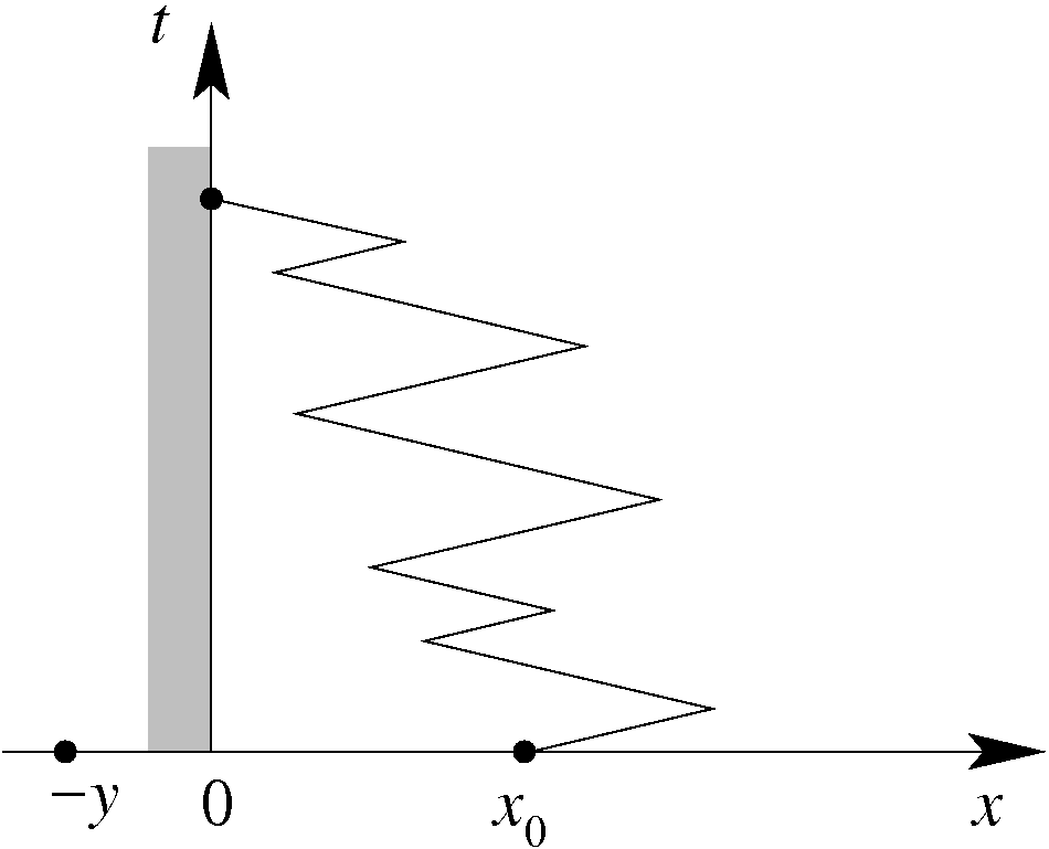
Figure 2: Persistent random walk with a trap at the origin. The random walker starts in $x=x_{0}$ and moves at constant speed $c$. It changes its direction at random times (Poisson distributed, with mean $\ell^{\star}/c$). The process stops when the random walker reaches the boundary at the origin. The time at which this event occurs is called the first-passage time at the origin. The point located at $-y$ (with $y>0$) is an intermediary used during the computation of the first passage time probability distribution.

We consider now the first-passage problem at the origin while the walk starts at $x_{0}>0$. To obtain the time distribution of the first arrival at the origin, we use Siegert’s formula [28] in the same way as Foong and Kanno did for the symmetric telegrapher’s equation [25]. We denote by $r_{1}(t\,|\,x_{0},\,\mathchoice{\leavevmode\hbox to7.13pt{\vbox to7.13pt{\text{[drawing]}}}}{\leavevmode\hbox to7.13pt{\vbox to7.13pt{\text{[drawing]}}}}{\leavevmode\hbox to5.5pt{\vbox to5.5pt{\text{[drawing]}}}}{\leavevmode\hbox to3.1pt{\vbox to3.1pt{\text{[drawing]}}}})$ the time probability distribution of the first passage at the origin of the random walker. Siegert’s formula states that, for any $y>0$

$$\hat{r}_{1}(s\,|\,x_{0},\,\mathchoice{\leavevmode\hbox to7.13pt{\vbox to7.13pt{\text{[drawing]}}}}{\leavevmode\hbox to7.13pt{\vbox to7.13pt{\text{[drawing]}}}}{\leavevmode\hbox to5.5pt{\vbox to5.5pt{\text{[drawing]}}}}{\leavevmode\hbox to3.1pt{\vbox to3.1pt{\text{[drawing]}}}})=\frac{\hat{p}(-x_{0}-y,\,s\,|\,\mathchoice{\leavevmode\hbox to7.13pt{\vbox to7.13pt{\text{[drawing]}}}}{\leavevmode\hbox to7.13pt{\vbox to7.13pt{\text{[drawing]}}}}{\leavevmode\hbox to5.5pt{\vbox to5.5pt{\text{[drawing]}}}}{\leavevmode\hbox to3.1pt{\vbox to3.1pt{\text{[drawing]}}}})}{\hat{p}(-y,\,s\,|\,\ominus)},$$ (24)

where $\hat{p}$ is the Laplace transform of the Green’s function $p$ as given by Equation (13). The first-passage time distribution has the dimension of an inverse time $\left[\mathrm{T}^{-1}\right]$. It follows from the fact that to reach the point $-y$ (see figure 2), the walker must first reach the origin and start from this point a random walk with initial velocity $-c$. We have readily

$$\hat{p}(x,\,s\,|\,\mathchoice{\leavevmode\hbox to7.13pt{\vbox to7.13pt{\text{[drawing]}}}}{\leavevmode\hbox to7.13pt{\vbox to7.13pt{\text{[drawing]}}}}{\leavevmode\hbox to5.5pt{\vbox to5.5pt{\text{[drawing]}}}}{\leavevmode\hbox to3.1pt{\vbox to3.1pt{\text{[drawing]}}}})=\frac{1}{2}\left(\frac{s+2\mu\mp\kappa}{\sqrt{(s+\mu)^{2}-1}}\pm\mathrm{sign}(x)\right)\mathrm{e}^{\kappa x-|x|\sqrt{(s+\mu)^{2}-1}}.$$ (25)

In the $\ominus$ case, the expression takes the simple form $\hat{r}_{1}(s\,|\,x_{0},\,\ominus)=\mathrm{e}^{-\kappa x_{0}-x_{0}\sqrt{(s+\mu)^{2}-1}}$ such that using the Equation (B.5) we obtain

$$r_{1}(t\,|\,x_{0},\,\ominus)=2x_{0}\,u_{1}(-x_{0},\,t)+\operatorname{\delta}(t-x_{0})\mathrm{e}^{-x_{0}/\ell^{\star}_{-}}.$$ (26)

We remark that the result does not depend on $y$, as should be expected. We should also notice that the result is made of direct contribution for the unscattered walkers and a term containing $u_{1}$ which accounts for an even number of scattering events. The counting statistics of the number of scattering events before reaching the origin is indeed obtained by replacing the functions in Siegert’s formula (24) by the generating functions $\overline{P}(\cdot,\,s,\,z\,|\mathchoice{\leavevmode\hbox to7.13pt{\vbox to7.13pt{\text{[drawing]}}}}{\leavevmode\hbox to7.13pt{\vbox to7.13pt{\text{[drawing]}}}}{\leavevmode\hbox to5.5pt{\vbox to5.5pt{\text{[drawing]}}}}{\leavevmode\hbox to3.1pt{\vbox to3.1pt{\text{[drawing]}}}})$ The generating function of the number of scattering events before reaching the origin is therefore $r_{z}/r_{1}$ with $r_{z}(t\,|\,x_{0},\,\ominus)=2x_{0}u_{z}(-x_{0},\,t\,|\,\ominus)$. (The Dirac delta function accounting for zero scattering events should be discarded in this expression for the same reasons as in the preceding section.)

The $\oplus$ case is handled by remarking that the expression (24) yields the symmetrical relation $\hat{r}(s\,|\,\oplus)=\hat{r}(s\,|\,\ominus)\big{(}s+\mu-\sqrt{(s+\mu)^{2}-1}\big{)}\ell^{\star}_{-}$. Invoking the identities (B.6) and (B.11) in the Appendix, we get

$$r_{z}(t\,|\,x_{0},\,\oplus)=\frac{2}{\ell^{\star}_{+}}\frac{x_{0}}{t+x_{0}}g_{z}(-x_{0},\,t)+\frac{2}{z\ell^{\star}_{+}}\frac{t-x_{0}}{t+x_{0}}u_{z}(-x_{0},\,t).$$ (27)

Some examples of first-passage time distributions are displayed in Figure 3

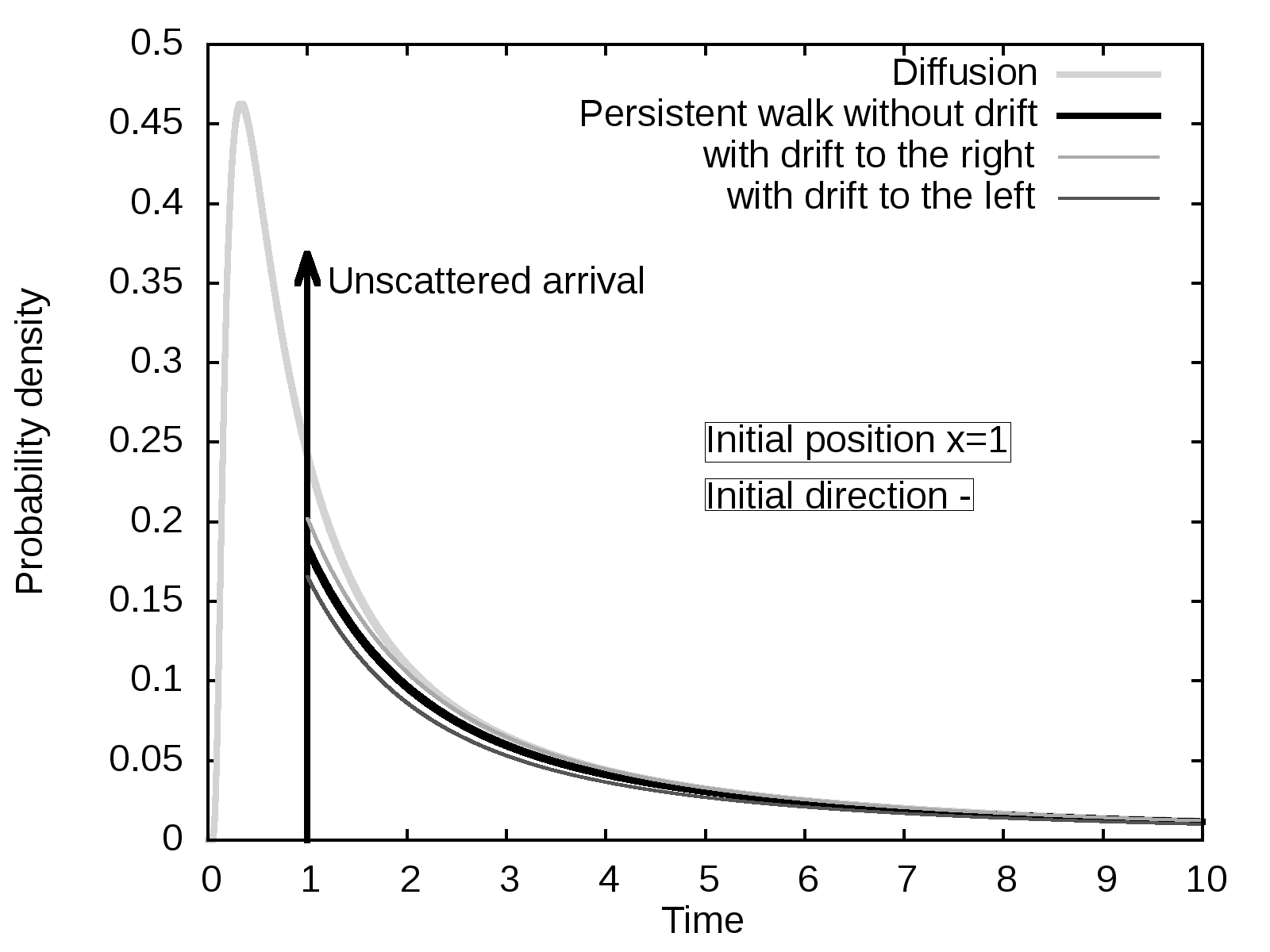
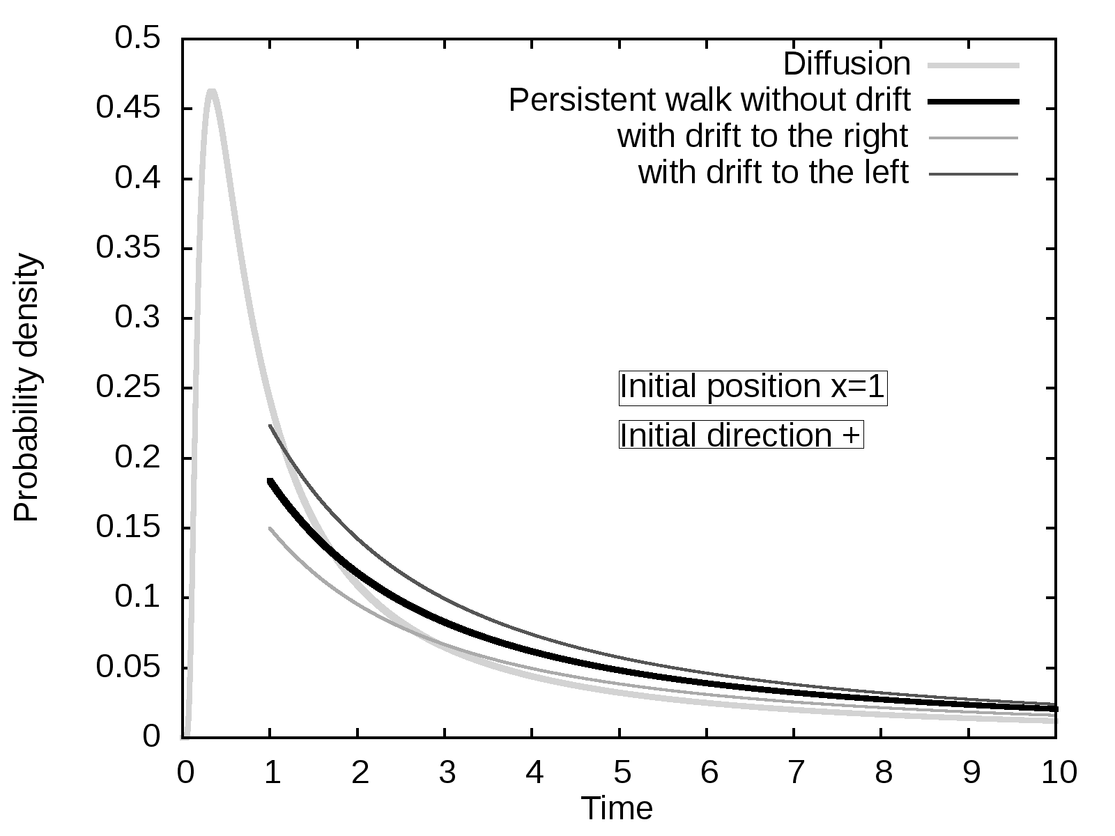
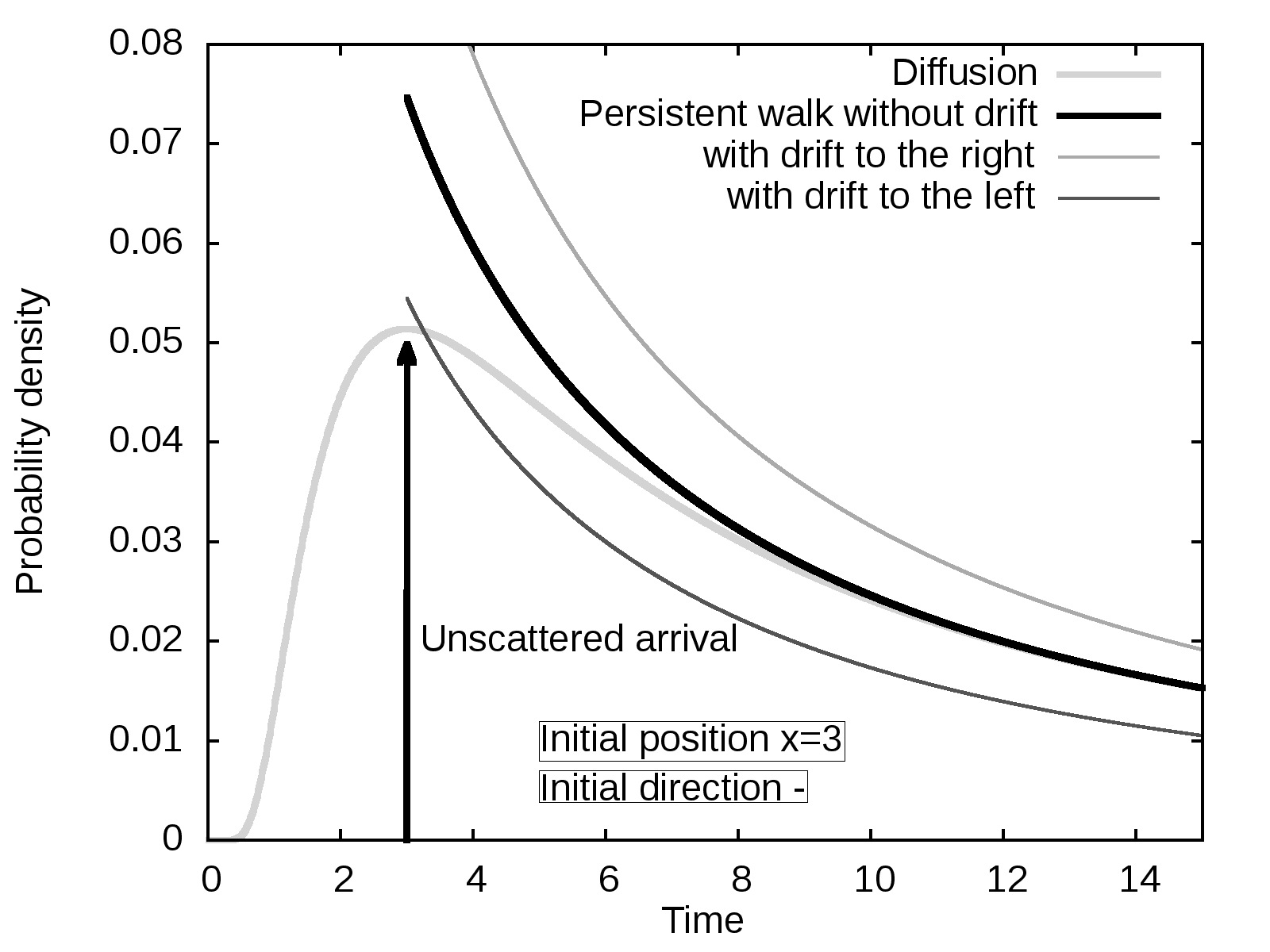
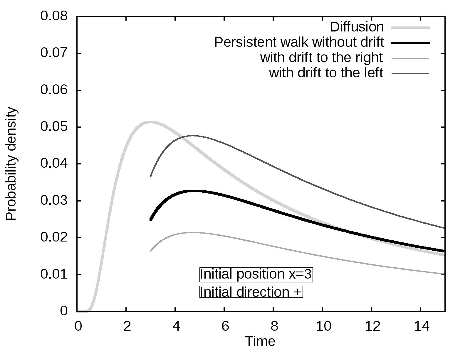
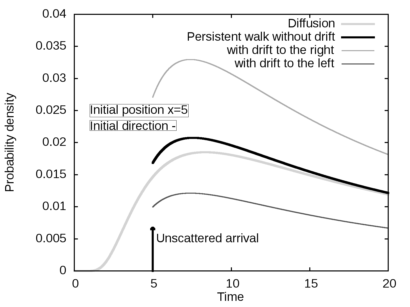
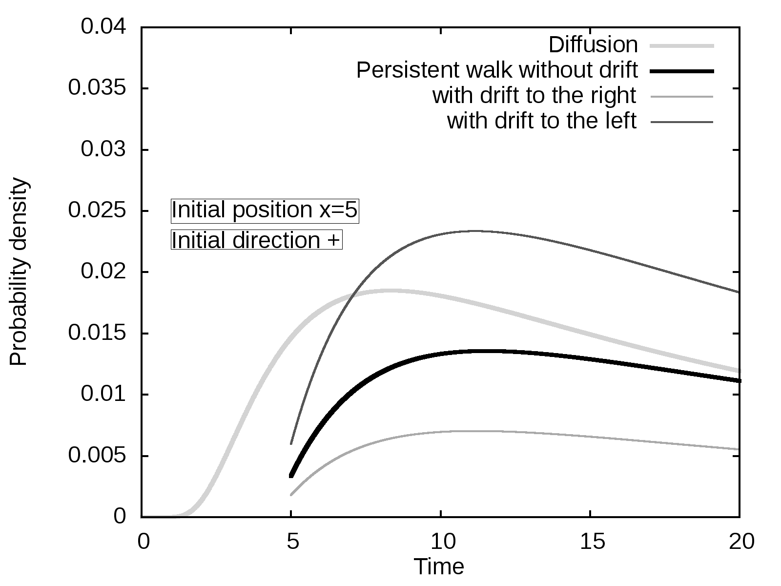
Figure 3: Comparison between the distribution of first passage time at the origin for a diffusion process and for a persistent random walk. The result shown without drift is the case $\kappa=0$, while the drifted ones correspond to the cases $\kappa=0.1$ and $\kappa=-0.1$ for the drift to the right and the drift to the left respectiveley. The processes start at $x_{0}=1$, $3$ and $5$ with initial direction $\ominus$ (left) or $\oplus$ (right). One observes the “direct” unscattered arrival of the persistent walk as a peak for initial direction $\ominus$. The units are fixed by $c=1$, $\ell^{\star}=1$ and $D=1=c\ell^{\star}$ is the diffusion constant of the diffusion process.

In the symmetric case $\kappa=0$, the first passage time distribution at a trap, or one of two traps, is conveniently provided by the method of images. This method can only yield solutions that are linear combinations of term of the form $p(x_{i},\,t\,|\,\mathchoice{\leavevmode\hbox to7.13pt{\vbox to7.13pt{\text{[drawing]}}}}{\leavevmode\hbox to7.13pt{\vbox to7.13pt{\text{[drawing]}}}}{\leavevmode\hbox to5.5pt{\vbox to5.5pt{\text{[drawing]}}}}{\leavevmode\hbox to3.1pt{\vbox to3.1pt{\text{[drawing]}}}})$ where several value of $x_{i}$ may be used. We deduce from this remark, that the solutions given by the method of images are solution of the differential equation (for instance the usual telegrapher’s equation). As soon as $\kappa\neq 0$, the results (26) and (27) are not solutions of the ATE, which means that the method of images can’t yield the previous results.

6.2 Phenomenology

In the case $\kappa\leq 0$, the walker will reach the origin almost surely, but it is interesting to notice that when $\kappa>0$, the walker has a finite probability of never reaching the origin, because of the effective drift due to the mean free path asymmetry. The probability that the walker reaches the origin is called the origin visit probability $\mathbb{P}_{\text{origin}}$. The computation of this probability is detailed in the Appendix. We find, for $\kappa>0$,

$$\mathbb{P}_{\text{origin}}(x_{0},\,\ominus) =\int_{0}^{\infty}r(t\,|\,x_{0},\,\ominus)\,\mathrm{d}t=\mathrm{e}^{-2\kappa x_{0}},$$ (28)

$$\mathbb{P}_{\text{origin}}(x_{0},\,\oplus) =\int_{0}^{\infty}r(t\,|\,x_{0},\,\oplus)\,\mathrm{d}t=\frac{\ell^{\star}_{-}}{\ell^{\star}_{+}}\mathrm{e}^{-2\kappa x_{0}}.$$ (29)

Let us consider the escape probability $\mathbb{P}_{\text{escape}}=1-\mathbb{P}_{\text{origin}}$ when $\kappa$ is close to zero. For $\kappa\leq 0$, $\mathbb{P}_{\text{escape}}=0$. For small $\kappa>0$, the slope of $\mathbb{P}_{\text{escape}}$ as a function of $\kappa$ is $2x_{0}$ for the $\ominus$ initial condition and $2(x_{0}+1)$ for the $\oplus$ initial condition. This means that for small $\kappa>0$, the difference between the two initial conditions is simply a “shift length” equal to $1=\ell^{\star}$, and most remarkably independent of $x_{0}$ : A random walk starting in the $\oplus$ direction at $x_{0}$ has the same probability of escape as a random walk starting in the direction $\ominus$ at $x_{0}+\ell^{\star}$. The parameter $\kappa$ plays a role similar to an order parameter in a phase transition.

The average time after which the origin is reached, $\mathbb{T}_{\text{origin}}(x_{0}\,|\,\mathchoice{\leavevmode\hbox to7.13pt{\vbox to7.13pt{\text{[drawing]}}}}{\leavevmode\hbox to7.13pt{\vbox to7.13pt{\text{[drawing]}}}}{\leavevmode\hbox to5.5pt{\vbox to5.5pt{\text{[drawing]}}}}{\leavevmode\hbox to3.1pt{\vbox to3.1pt{\text{[drawing]}}}})$ is infinite in the case $\kappa\geq 0$, but it becomes finite in the case $\kappa<0$, also experiencing a “transition”. Its value is easily obtained using the relation

$$\mathbb{T}_{\text{origin}}(x_{0}\,|\,\mathchoice{\leavevmode\hbox to7.13pt{\vbox to7.13pt{\text{[drawing]}}}}{\leavevmode\hbox to7.13pt{\vbox to7.13pt{\text{[drawing]}}}}{\leavevmode\hbox to5.5pt{\vbox to5.5pt{\text{[drawing]}}}}{\leavevmode\hbox to3.1pt{\vbox to3.1pt{\text{[drawing]}}}})=\int_{0}^{\infty}t\,r_{1}(t\,|\,x_{0},\,\mathchoice{\leavevmode\hbox to7.13pt{\vbox to7.13pt{\text{[drawing]}}}}{\leavevmode\hbox to7.13pt{\vbox to7.13pt{\text{[drawing]}}}}{\leavevmode\hbox to5.5pt{\vbox to5.5pt{\text{[drawing]}}}}{\leavevmode\hbox to3.1pt{\vbox to3.1pt{\text{[drawing]}}}})\,\mathrm{d}t=\left(-\vphantom{\lim_{x}}\partial_{s}{}\hat{r}_{1}(s\,|\,x_{0},\,\mathchoice{\leavevmode\hbox to7.13pt{\vbox to7.13pt{\text{[drawing]}}}}{\leavevmode\hbox to7.13pt{\vbox to7.13pt{\text{[drawing]}}}}{\leavevmode\hbox to5.5pt{\vbox to5.5pt{\text{[drawing]}}}}{\leavevmode\hbox to3.1pt{\vbox to3.1pt{\text{[drawing]}}}})\right)_{s=0}.$$

We obtain $\mathbb{T}_{\text{origin}}(x_{0}\,|\,\oplus)=\mathbb{T}_{\text{origin}}(x_{0}\,|\,\ominus)+\frac{1}{|\kappa|}=\frac{x_{0}\mu+1}{|\kappa|}$. In this expression we observe an effective fixed delay equal to $1/|\kappa|$ for the walker starting in direction $\oplus$ to find itself in the same condition as if it started in the direction $\ominus$. We may call it a “flip delay”. The average time for a start in the $\ominus$ direction is proportionnal to $x_{0}$, showing that the effective movement is uniform at an effective speed $|\kappa|/\mu$. In the case $\kappa$, all the higher moments of the first-time passage are also finite and computed using the same technique as for $\mathbb{T}_{\text{origin}}$. We can for instance compute the fluctuations $\mathbb{T}^{(2)}_{\text{origin}}$ of the first-time passage at the origin and we find

$$\mathbb{T}^{(2)}_{\text{origin}}(x_{0}\,|\,\oplus)=\mathbb{T}^{(2)}_{\text{origin}}(x_{0}\,|\,\ominus)+\frac{\mu}{|\kappa|^{3}}=\frac{x_{0}+\mu}{|\kappa|^{3}}.$$

We read in this result the fluctuations of the flip delay as $\mu/|\kappa|^{3}$ together with the fluctuations of the uniform movement duration $x_{0}/|\kappa|^{3}$.

6.3 A remark concerning the distributions of extrema

From the statistics of first passage times, it is possible to deduce the joint probability of the minimum and maximum values of the position $x$ during a persistent random walk of duration $t$, as it was first shown by Masoliver and Weiss [27]. We start by remarking that the probability that the minimum absciss reached by the walker during a time $t$ is greater than zero is equal to the probability that the walker does not reach the origin during this time interval :

$$\mathbb{P}\left[\text{the minimal absciss reached during}\;[0,\,t]\;\text{is}\;\geq 0\,\vrule\;x_{0},\,\mathchoice{\leavevmode\hbox to7.13pt{\vbox to7.13pt{\text{[drawing]}}}}{\leavevmode\hbox to7.13pt{\vbox to7.13pt{\text{[drawing]}}}}{\leavevmode\hbox to5.5pt{\vbox to5.5pt{\text{[drawing]}}}}{\leavevmode\hbox to3.1pt{\vbox to3.1pt{\text{[drawing]}}}}\right]=1-\int_{0}^{t}r_{1}(t^{\prime}\,|\,x_{0},\,\mathchoice{\leavevmode\hbox to7.13pt{\vbox to7.13pt{\text{[drawing]}}}}{\leavevmode\hbox to7.13pt{\vbox to7.13pt{\text{[drawing]}}}}{\leavevmode\hbox to5.5pt{\vbox to5.5pt{\text{[drawing]}}}}{\leavevmode\hbox to3.1pt{\vbox to3.1pt{\text{[drawing]}}}})\,\,\mathrm{d}t^{\prime}.$$

This setup is equivalent to the situation where the walker starts from the origin and reaches a negative minimum $-x$ (with $x>0$). By derivation with respect to $x$ we find that the spatial distribution of the minimum absciss reached by a walker starting at the origin is

$$m(-x\,|\,t,\,\mathchoice{\leavevmode\hbox to7.13pt{\vbox to7.13pt{\text{[drawing]}}}}{\leavevmode\hbox to7.13pt{\vbox to7.13pt{\text{[drawing]}}}}{\leavevmode\hbox to5.5pt{\vbox to5.5pt{\text{[drawing]}}}}{\leavevmode\hbox to3.1pt{\vbox to3.1pt{\text{[drawing]}}}})=\int_{0}^{t}\partial_{x}{}r_{1}(t^{\prime}\,|\,x,\,\mathchoice{\leavevmode\hbox to7.13pt{\vbox to7.13pt{\text{[drawing]}}}}{\leavevmode\hbox to7.13pt{\vbox to7.13pt{\text{[drawing]}}}}{\leavevmode\hbox to5.5pt{\vbox to5.5pt{\text{[drawing]}}}}{\leavevmode\hbox to3.1pt{\vbox to3.1pt{\text{[drawing]}}}})\,\,\mathrm{d}t^{\prime}\qquad(x>0).$$ (30)

For $x>0$, we have of course $m(x\,|\,t)=0$. The distribution of the maximum position is obtained from the same formula, by remarking that it is the symmetric distribution obtained with the opposite sign of $\kappa$. Note that for $\kappa\neq 0$, the expression (30) cannot be expressed in terms of the elementary functions $g_{1}$ and $u_{1}$, a numerical approach is thus required.

7 First-passage statistics in a finite interval

The first-passage time distributions we have obtained in the preceding section have been obtained thank to Siegert’s relation, a technique only valid for a single boundary problem. The asymmetric persistent random walk in a finite interval presents mathematical difficulties with regard to the full first-passage distribution. It is nonetheless possible to derive some relevant time integrated statistical properties such as the splitting probabilities and the mean exit time. These quantities can be obtained by very general methods which realisations do not present any new difficulty here.

We consider the random walk in the interval $[0,\,L]$. In the steady state $p^{+}$ and $p^{-}$ are by definition independent of the time and also independent of the initial condition, position and direction of propagation. The equations (3) reduce to

$$\partial_{x}{j}=0\qquad\partial_{x}{p}=-2\mu j+2\kappa p.$$ (31)

The stationnary current is obviously uniformly equal to $0$ and the stationnary distribution is immediately obtained, after normalization, as

$$p_{\rm ss}(x)=\frac{2\kappa}{\mathrm{e}^{2\kappa L}-1}\,\mathrm{e}^{2\kappa x}.$$ (32)

7.1 Splitting probabilities

We consider the splitting probabilities $q(x\,|\,\mathchoice{\leavevmode\hbox to7.13pt{\vbox to7.13pt{\text{[drawing]}}}}{\leavevmode\hbox to7.13pt{\vbox to7.13pt{\text{[drawing]}}}}{\leavevmode\hbox to5.5pt{\vbox to5.5pt{\text{[drawing]}}}}{\leavevmode\hbox to3.1pt{\vbox to3.1pt{\text{[drawing]}}}})$ that the walker starting at position $x$ in the direction reaches the origin at $x=0$ before ever visiting the other end of the interval at $x=L$. In a model where the walker escapes irreversibly from the interval whenever it reaches any of the two ends, $q$ is the probability that the walker escapes from $x=0$. Consider a trajectory starting at $x$ in the direction $\oplus$. It has a probability $q(x\,|\,\oplus)$ of reaching the origin first. After a short time $\Delta t$, the walker can either be still moving in the $\oplus$ direction or moving in the opposite direction and having reached the position $x+\Delta x^{\prime}$ where $|\Delta x^{\prime}|\leq c\Delta t$. The probability $q(x\,|\,\oplus)$ is therefore equal to

$$q(x\,|\,\oplus)=\left(1-\frac{c\Delta t}{\ell^{\star}_{+}}\right)q(x+c\Delta t\,|\,\oplus)+\frac{c\Delta t}{\ell^{\star}_{-}}q(x+\Delta x^{\prime}\,|\,\ominus).$$ (33)

Taking the first order in $\Delta t$ and proceeding in the same way with the initial condition $\ominus$ we obtain the backward Kolmogorov equations

$$\partial_{x}{}q(x\,|\,\oplus)=\partial_{x}{}q(x\,|\,\ominus)=\frac{q(x\,|\,\oplus)}{\ell^{\star}_{+}}-\frac{q(x\,|\,\ominus)}{\ell^{\star}_{-}}.$$ (34)

The boundary conditions for these functions are $q(0\,|\,\ominus)=1$ and $q(L\,|\,\oplus)=0$. The solutions of the equations (34) are of the form $q(x\,|\mathchoice{\leavevmode\hbox to7.13pt{\vbox to7.13pt{\text{[drawing]}}}}{\leavevmode\hbox to7.13pt{\vbox to7.13pt{\text{[drawing]}}}}{\leavevmode\hbox to5.5pt{\vbox to5.5pt{\text{[drawing]}}}}{\leavevmode\hbox to3.1pt{\vbox to3.1pt{\text{[drawing]}}}})=A_{\pm}\mathrm{e}^{-2\kappa x}+B_{\pm}$. The boundary conditions provide two relations between the integration constants, $A_{+}\mathrm{e}^{-2\kappa L}+B_{+}=0$ and $A_{-}+B_{-}=1$, while the Kolmogorov equations provide two further relations $A_{+}=A_{-}$ and $B_{+}/\ell^{\star}_{+}=B_{-}/\ell^{\star}_{-}$. This is enough to get the splitting probabilities

$$q(x\,|\,\mathchoice{\leavevmode\hbox to7.13pt{\vbox to7.13pt{\text{[drawing]}}}}{\leavevmode\hbox to7.13pt{\vbox to7.13pt{\text{[drawing]}}}}{\leavevmode\hbox to5.5pt{\vbox to5.5pt{\text{[drawing]}}}}{\leavevmode\hbox to3.1pt{\vbox to3.1pt{\text{[drawing]}}}})=\frac{\ell^{\star}_{+}\mathrm{e}^{-2\kappa x}-\ell^{\star}_{\pm}\mathrm{e}^{-2\kappa L}}{\ell^{\star}_{+}-\ell^{\star}_{-}\mathrm{e}^{-2\kappa L}}.$$ (35)

Interestingly, the difference between these probabilities is uniform $q(x\,|\,\ominus)-q(x\,|\,\oplus)=2\kappa\mathrm{e}^{-2\kappa L}/(\ell^{\star}_{+}-\ell^{\star}_{-}\exp(-2\kappa L))$ that we interpret as the probabilistic advantage to start moving towards the origin.

7.2 Mean exit time

Since the walker exits the interval $[0,\,L]$ with probability 1, it is interesting to know how long it takes on average to exit the interval. We denote by $\mathbb{T}_{\text{exit}}(x\,|\,\mathchoice{\leavevmode\hbox to7.13pt{\vbox to7.13pt{\text{[drawing]}}}}{\leavevmode\hbox to7.13pt{\vbox to7.13pt{\text{[drawing]}}}}{\leavevmode\hbox to5.5pt{\vbox to5.5pt{\text{[drawing]}}}}{\leavevmode\hbox to3.1pt{\vbox to3.1pt{\text{[drawing]}}}})$ the average time taken by a walker starting from the position $x$ and moving in the direction . Let us proceed as for the splitting probabilities and consider a walker located at $x$ moving in the direction $\oplus$. After a time interval $\Delta t$ the mean exit time has been reduced by $\Delta t$ and the walker can either be still moving in the $\oplus$ direction or moving in the opposite direction and having reached another position $x+\Delta x^{\prime}$ where $|\Delta x^{\prime}|\leq c\Delta t$. The mean exit times are related by

$$\mathbb{T}_{\text{exit}}(x\,|\,\oplus)=\Delta t+\left(1-\frac{c\Delta t}{\ell^{\star}_{+}}\right)\mathbb{T}_{\text{exit}}(x+c\Delta t\,|\,\oplus)+\frac{c\Delta t}{\ell^{\star}_{-}}\mathbb{T}_{\text{exit}}(x+\Delta x^{\prime}\,|\,\ominus).$$ (36)

Applying the same reasoning with the initial condition $\ominus$, we obtain the backward Fokker-Planck equations

$$\partial_{x}{}\mathbb{T}_{\text{exit}}(x\,|\,\mathchoice{\leavevmode\hbox to7.13pt{\vbox to7.13pt{\text{[drawing]}}}}{\leavevmode\hbox to7.13pt{\vbox to7.13pt{\text{[drawing]}}}}{\leavevmode\hbox to5.5pt{\vbox to5.5pt{\text{[drawing]}}}}{\leavevmode\hbox to3.1pt{\vbox to3.1pt{\text{[drawing]}}}})=\frac{\mathbb{T}_{\text{exit}}(x\,|\,\oplus)}{\ell^{\star}_{+}}-\frac{\mathbb{T}_{\text{exit}}(x\,|\,\ominus)}{\ell^{\star}_{-}}\mp 1$$ (37)

with the boundary conditions $\mathbb{T}_{\text{exit}}(0\,|\,\ominus)=\mathbb{T}_{\text{exit}}(L\,|\,\oplus)=0$. The solution of these coupled differential equations follows teh same steps as the computation of $q(x\,|\,\mathchoice{\leavevmode\hbox to7.13pt{\vbox to7.13pt{\text{[drawing]}}}}{\leavevmode\hbox to7.13pt{\vbox to7.13pt{\text{[drawing]}}}}{\leavevmode\hbox to5.5pt{\vbox to5.5pt{\text{[drawing]}}}}{\leavevmode\hbox to3.1pt{\vbox to3.1pt{\text{[drawing]}}}})$ and we obtain the expressions

$$\mathbb{T}_{\text{exit}}(x\,|\,\oplus)=\frac{(\ell^{\star}_{+})^{2}(L-x)+(x+\mu)\mathrm{e}^{-2\kappa L}-(L+\mu)\mathrm{e}^{-2\kappa x}}{\kappa\ell^{\star}_{+}-\kappa\ell^{\star}_{-}\mathrm{e}^{-2\kappa L}}.$$ (38)

8 Concluding remarks

Recensing all possible symmetry breaking for the one-dimensional persistent random walks, we have focused our efforts on the only case leading new physical results, the case of mean free path anisotropy. This case is physically relevant in, for instance, microtubule growth. Statistical quantities such as the Green’s function, the generating function of the number of scattering events, the first-passage statistics are obtained from standard computation techniques.

However, one of the first-passage time distributions obtained in the asymmetric case, the Equation (27), cannot be obtained by the simplest, standard method used in the symmetric case, even though a closed form was found. This shows that the asymmetric case $\kappa\neq 0$ describes a new physical situation, not present in the symmetric case. In this situation the probability of return at the origin is strictly less than 1, so we may speak of a recurrent-transient transition (second order) at $\kappa=0$. We also remarked that for $\kappa\neq 0$ some statistical distributions do not even have exact analytical forms. The case $\kappa=0$ is indeed peculiar, because $\mathbb{P}_{\text{escape}}=0$ and $\mathbb{T}_{\text{origin}}$ is infinite, whereas in the case where $\kappa\neq 0$ either $\mathbb{P}_{\text{escape}}$ or $\mathbb{T}_{\text{origin}}$ takes a finite value.

All along the text, we have distinguished the walk by the initial direction of propagation $\oplus$ or $\ominus$ and we have observed that the results strongly differ depending on it. As Dunkel and Hänggi noted, the persistent random walk is not a Markov process [15]. If indeed one takes the initial direction of propagation as a random variable with $\mathbb{P}(\oplus)+\mathbb{P}(\ominus)=1/2$, then the net initial current is $j=0$. At a time $t>0$ the current is generally not equal to zero, which means that the propagator from time $t$ to a time $t^{\prime}>t$ does not have the same initial condition for current as at time $t=0$. However, we must observe that the process’s construction implies that the Markovian property is restored if one considers the directions of propagation separately. Chapman-Kolmogorov relations follow as

$$\sum_{\sigma=\oplus,\ominus}\int p^{\beta}(y-x,\,t_{1}\,|\,\sigma)\,p^{\sigma}(x,\,t_{2}\,|\,\alpha)\;\,\mathrm{d}x=p^{\beta}(y,\,t_{1}+t_{2}\,|\,\alpha),$$

where $\alpha$, $\beta$ and $\sigma$ stand for signs $\oplus$ or $\ominus$ and $p^{\pm}$ functions are given by the Equations (16) and (17).

We have not investigated the situation where $\kappa\neq 0$ in the presence of a speed asymmetry. The position spatial distribution in this situation follows straightforwardly from this work, but the first-passage time distributions do not. Even though the effects of both asymmetries separately are drifts of the average position of the walker along time, these asymmetries cannot be reconciled into a single one, because the speed asymmetry is a relativistic change of referential and the asymmetry $\kappa\neq 0$ cannot be reduced to such a change. The evidence for this impossiblity is provided by the fact that the first-passage time distributions are not solutions of the ATE for $\kappa\neq 0$, as explained in Section 6, although from the linearity of the change of reference frame, they are solutions of the ATE in the case of speed asymmetry.

The results of this work may find applications in the domains where the telegrapher’s equation is relevant, extended to the situations where a scattering asymmetry is present. The phenomenology of the first-passage time, introducing the shift length and the flip delay between two walkers starting in opposite directions, may prove useful to interpret experiments in biophysics, optics.

Aknowledgments

I would like to thank Josh Myers for our fruitful discussions and Sidney Redner for his nice suggestions.

Appendix A Counting statistics of the $\oplus$ and $\ominus$ walkers

The counting statistics fot the walkers that in the states $\oplus$ or $\ominus$ at time $t$ are obtained from the same algebraic derivations written in Section 5.

$$\overline{P}^{\pm}(z\,|\,x,\,t\,|\,\mathchoice{\leavevmode\hbox to7.13pt{\vbox to7.13pt{\text{[drawing]}}}}{\leavevmode\hbox to7.13pt{\vbox to7.13pt{\text{[drawing]}}}}{\leavevmode\hbox to5.5pt{\vbox to5.5pt{\text{[drawing]}}}}{\leavevmode\hbox to3.1pt{\vbox to3.1pt{\text{[drawing]}}}}) =\frac{u_{z}(x,\,t)}{u_{1}(x,\,t)}$$ (A.1)

$$\left\langle{n^{\pm}(x,\,t\,|\,\mathchoice{\leavevmode\hbox to7.13pt{\vbox to7.13pt{\text{[drawing]}}}}{\leavevmode\hbox to7.13pt{\vbox to7.13pt{\text{[drawing]}}}}{\leavevmode\hbox to5.5pt{\vbox to5.5pt{\text{[drawing]}}}}{\leavevmode\hbox to3.1pt{\vbox to3.1pt{\text{[drawing]}}}})}\right\rangle =\frac{g_{1}(x,\,t)}{u_{1}(x,\,t)}$$ (A.2)

$$\big{(}\Delta n^{\pm}(x,\,t\,|\,\mathchoice{\leavevmode\hbox to7.13pt{\vbox to7.13pt{\text{[drawing]}}}}{\leavevmode\hbox to7.13pt{\vbox to7.13pt{\text{[drawing]}}}}{\leavevmode\hbox to5.5pt{\vbox to5.5pt{\text{[drawing]}}}}{\leavevmode\hbox to3.1pt{\vbox to3.1pt{\text{[drawing]}}}})^{2}\big{)} =(t^{2}-x^{2})+2\frac{g_{1}(x,\,t)}{u_{1}(x,\,t)}-\frac{g_{1}(x,\,t)^{2}}{u_{1}(x,\,t)^{2}}$$ (A.3)

$$\overline{P}^{\mp}(z\,|\,x,\,t\,|\,\mathchoice{\leavevmode\hbox to7.13pt{\vbox to7.13pt{\text{[drawing]}}}}{\leavevmode\hbox to7.13pt{\vbox to7.13pt{\text{[drawing]}}}}{\leavevmode\hbox to5.5pt{\vbox to5.5pt{\text{[drawing]}}}}{\leavevmode\hbox to3.1pt{\vbox to3.1pt{\text{[drawing]}}}}) =\frac{g_{z}(x,\,t)}{g_{1}(x,\,t)}$$ (A.4)

$$\left\langle{n^{\mp}(x,\,t\,|\,\mathchoice{\leavevmode\hbox to7.13pt{\vbox to7.13pt{\text{[drawing]}}}}{\leavevmode\hbox to7.13pt{\vbox to7.13pt{\text{[drawing]}}}}{\leavevmode\hbox to5.5pt{\vbox to5.5pt{\text{[drawing]}}}}{\leavevmode\hbox to3.1pt{\vbox to3.1pt{\text{[drawing]}}}})}\right\rangle =1+(t^{2}-x^{2})\frac{u_{1}(x,\,t)}{g_{1}(x,\,t)}$$ (A.5)

$$\big{(}\Delta n^{\mp}(x,\,t\,|\,\mathchoice{\leavevmode\hbox to7.13pt{\vbox to7.13pt{\text{[drawing]}}}}{\leavevmode\hbox to7.13pt{\vbox to7.13pt{\text{[drawing]}}}}{\leavevmode\hbox to5.5pt{\vbox to5.5pt{\text{[drawing]}}}}{\leavevmode\hbox to3.1pt{\vbox to3.1pt{\text{[drawing]}}}})^{2}\big{)} =(t^{2}-x^{2})\left[1-(t^{2}-x^{2})\frac{u_{1}(x,\,t)^{2}}{g_{1}(x,\,t)^{2}}\right]$$ (A.6)

From these expressions, we obtain some statistical bounds, using the positivity of $(\Delta n^{\pm})^{2}$. From the equations (A.2) and (A.3) we get a higher bound for $\left\langle{n^{\pm}(x,\,t\,|\,\mathchoice{\leavevmode\hbox to7.13pt{\vbox to7.13pt{\text{[drawing]}}}}{\leavevmode\hbox to7.13pt{\vbox to7.13pt{\text{[drawing]}}}}{\leavevmode\hbox to5.5pt{\vbox to5.5pt{\text{[drawing]}}}}{\leavevmode\hbox to3.1pt{\vbox to3.1pt{\text{[drawing]}}}})}\right\rangle$ and from (A.5) and (A.6) a higher bound for $\left\langle{n^{\mp}(x,\,t\,|\,\mathchoice{\leavevmode\hbox to7.13pt{\vbox to7.13pt{\text{[drawing]}}}}{\leavevmode\hbox to7.13pt{\vbox to7.13pt{\text{[drawing]}}}}{\leavevmode\hbox to5.5pt{\vbox to5.5pt{\text{[drawing]}}}}{\leavevmode\hbox to3.1pt{\vbox to3.1pt{\text{[drawing]}}}})}\right\rangle$. Remarking that (A.2) and (A.5) provide also the relation $(\left\langle{n^{\pm}}\right\rangle-1)\left\langle{n^{\mp}}\right\rangle=t^{2}-x^{2}$ we have the following bounds

$$1+\frac{t^{2}-x^{2}}{1+\sqrt{t^{2}-x^{2}}} \leq\left\langle{n^{\pm}(x,\,t\,|\,\mathchoice{\leavevmode\hbox to7.13pt{\vbox to7.13pt{\text{[drawing]}}}}{\leavevmode\hbox to7.13pt{\vbox to7.13pt{\text{[drawing]}}}}{\leavevmode\hbox to5.5pt{\vbox to5.5pt{\text{[drawing]}}}}{\leavevmode\hbox to3.1pt{\vbox to3.1pt{\text{[drawing]}}}})}\right\rangle\leq 1+\sqrt{1+t^{2}-x^{2}}$$ (A.7)

$$\frac{t^{2}-x^{2}}{\sqrt{1+t^{2}-x^{2}}} \leq\left\langle{n^{\mp}(x,\,t\,|\mathchoice{\leavevmode\hbox to7.13pt{\vbox to7.13pt{\text{[drawing]}}}}{\leavevmode\hbox to7.13pt{\vbox to7.13pt{\text{[drawing]}}}}{\leavevmode\hbox to5.5pt{\vbox to5.5pt{\text{[drawing]}}}}{\leavevmode\hbox to3.1pt{\vbox to3.1pt{\text{[drawing]}}}})}\right\rangle\leq 1+\sqrt{t^{2}-x^{2}}.$$ (A.8)

Appendix B The functions $g_{z}$ and $u_{z}$ and their properties

B.1 Definitions

$$g_{z}(x,\,t) =z\frac{\mathrm{e}^{\kappa x-\mu t}}{2}I_{0}\left(z\sqrt{t^{2}-{x}^{2}}\right)\Theta(t-|x|)$$ (B.1)

$$u_{z}(x,\,t) =z\frac{\mathrm{e}^{\kappa x-\mu t}}{2}\frac{I_{1}\left(z\sqrt{t^{2}-{x}^{2}}\right)}{\sqrt{t^{2}-{x}^{2}}}\Theta(t-|x|)$$ (B.2)

B.2 Transforms

$$\frac{z}{(s+\mu)^{2}+(k-\mathrm{i}\kappa)^{2}-z^{2}} =\hat{\tilde{g}}_{z}(k,\,s)$$ (B.3)

$$z\frac{\mathrm{e}^{\kappa x-|x|\sqrt{(s+\mu)^{2}-z^{2}}}}{\sqrt{(s+\mu)^{2}-z^{2}}} =2\hat{g}_{z}(x,\,s)$$ (B.4)

$$\mathrm{e}^{\kappa x-|x|\sqrt{(s+\mu)^{2}-z^{2}}} =-2|x|\,\hat{u}_{z}(x,\,s)+\mathrm{e}^{\kappa x-(s+\mu)\,|x|}$$ (B.5)

$$\mathrm{e}^{\kappa x-|x|\sqrt{(s+\mu)^{2}-z^{2}}}\sqrt{(s+\mu)^{2}-z^{2}}=\\ 2z\hat{u}_{z}(x,\,s)-2\kappa x\hat{u}_{z}(x,\,s)+2x\partial_{x}{\hat{u}_{z}}(x,\,s)+\mathrm{sign}(x)(s+\mu)\mathrm{e}^{\kappa x-(s+\mu)|x|}$$ (B.6)

B.3 Derivatives

$$\partial_{t}{g_{z}}(x,t) =-\mu g_{z}(x,t)+zt\;u_{z}(x,t)+\frac{1}{2}\operatorname{\delta}(t-x)\mathrm{e}^{-t/\ell^{\star}_{+}}+\frac{1}{2}\operatorname{\delta}(t+x)\mathrm{e}^{-t/\ell^{\star}_{-}},$$ (B.7)

$$\partial_{x}{g_{z}}(x,t) =\kappa g_{z}(x,t)-zx\;u_{z}(x,t)-\frac{1}{2}\operatorname{\delta}(t-x)\mathrm{e}^{-t/\ell^{\star}_{+}}+\frac{1}{2}\operatorname{\delta}(t+x)\mathrm{e}^{-t/\ell^{\star}_{-}},$$ (B.8)

$$\partial_{z}{g_{z}}(x,t) =\frac{1}{z}g_{z}(x,t)+(t^{2}-x^{2})u_{z}(x,t),$$ (B.9)

$$\partial_{t}{u_{z}}(x,t) =-\mu u_{z}(x,t)+\frac{zt}{t^{2}-x^{2}}(g_{z}(x,t)-2u_{z}(x,t))+\frac{1}{4}\operatorname{\delta}(t-x)\mathrm{e}^{-t/\ell^{\star}_{+}}+\frac{1}{4}\operatorname{\delta}(t+x)\mathrm{e}^{-t/\ell^{\star}_{-}},$$ (B.10)

$$\partial_{x}{u_{z}}(x,t) =\kappa u_{z}(x,t)-\frac{zx}{t^{2}-x^{2}}(g_{z}(x,t)-2u_{z}(x,t))-\frac{1}{4}\operatorname{\delta}(t-x)\mathrm{e}^{-t/\ell^{\star}_{+}}+\frac{1}{4}\operatorname{\delta}(t+x)\mathrm{e}^{-t/\ell^{\star}_{-}},$$ (B.11)

$$\partial_{z}{u_{z}}(x,t) =g_{z}(x,t).$$ (B.12)

We have used the identity $I_{2}(x)=I_{0}(x)-\frac{2}{x}I_{1}(x)$.

Appendix C Probability of reaching the origin

Let us first compute $\mathbb{P}_{\text{origin}}(x_{0},\,\ominus)$ by remarking that it is the value of the Laplace transform of $r$ at $s=0$ :

$$\begin{split}\mathbb{P}_{\text{origin}}(x_{0},\,\ominus)&=\int_{0}^{\infty}r_{1}(t\,|\,x_{0},\,\ominus)\,\mathrm{d}t=\int_{0}^{\infty}\left[2x_{0}u_{1}(-x_{0},\,t)+\operatorname{\delta}(t-x_{0})\mathrm{e}^{-x_{0}/\ell^{\star}_{-}}\right]\,\mathrm{d}t\\ &=2x_{0}\,\hat{u}_{1}(-x_{0},\,0)+\mathrm{e}^{-x_{0}/\ell^{\star}_{-}}=\mathrm{e}^{-\kappa x_{0}-x_{0}|\kappa|}-\mathrm{e}^{-\kappa x_{0}-\mu x_{0}}+\mathrm{e}^{-x_{0}/\ell^{\star}_{-}}=\mathrm{e}^{(-\kappa-|\kappa|)x_{0}}\end{split}$$

and observe that the probability is equal to $1$ for $\kappa<0$ and strictly $<1$ for $\kappa>0$. The computation of $\mathbb{P}_{\text{origin}}(x_{0},\,\ominus)$ requires more work :

$$\begin{split}\mathbb{P}_{\text{origin}}(x_{0},\,\oplus)&=\int_{0}^{\infty}r_{1}(t\,|\,x_{0},\,\oplus)\,\mathrm{d}t\\ &=\int_{0}^{\infty}\frac{1}{\ell^{\star}_{+}}\left[\frac{x_{0}}{t+x_{0}}\mathrm{e}^{-\kappa x_{0}-\mu t}I_{0}\left(\sqrt{t^{2}-x_{0}^{2}}\right)+\frac{t-x_{0}}{t+x_{0}}\mathrm{e}^{-\kappa x_{0}-\mu t}\frac{2I_{1}\left(\sqrt{t^{2}-x_{0}^{2}}\right)}{2\sqrt{t^{2}-x_{0}^{2}}}\right]\,\mathrm{d}t\end{split}$$

Using the identity $\frac{x_{0}}{t+x_{0}}=\frac{1}{2}-\frac{1}{2}\frac{t-x_{0}}{t+x_{0}}$ this expression rewrites

$$\begin{split}\mathbb{P}_{\text{origin}}(x_{0},\,\oplus)&=\frac{\mathrm{e}^{-\kappa x_{0}}}{\ell^{\star}_{+}}\int_{0}^{\infty}\mathrm{e}^{-\mu t}\frac{1}{2}\frac{t-x_{0}}{t+x_{0}}\left[-I_{0}\left(\sqrt{t^{2}-x_{0}^{2}}\right)+2\frac{I_{1}\left(\sqrt{t^{2}-x_{0}^{2}}\right)}{\sqrt{t^{2}-x_{0}^{2}}}\right]\,\mathrm{d}t\;\cdots\\ &\quad\qquad\cdots+\frac{\mathrm{e}^{-\kappa x_{0}}}{2\ell^{\star}_{+}}\int_{0}^{\infty}\mathrm{e}^{-\mu t}I_{0}\left(\sqrt{t^{2}-x_{0}^{2}}\right)\,\mathrm{d}t\\ &=\frac{\mathrm{e}^{-\kappa x_{0}}}{2\ell^{\star}_{+}}\frac{\mathrm{e}^{-x_{0}\sqrt{\mu^{2}-1}}}{\sqrt{\mu^{2}-1}}-\frac{\mathrm{e}^{-\kappa x_{0}}}{2\ell^{\star}_{+}}\int_{0}^{\infty}\mathrm{e}^{-\mu t}\frac{t-x_{0}}{t+x_{0}}I_{2}\left(\sqrt{t^{2}-x_{0}^{2}}\right)\,\mathrm{d}t.\end{split}$$

The integral is the Laplace transform 4.17(11) in the table [29] for the case $\nu=2$ such that we obtain

$$\mathbb{P}_{\text{origin}}(x_{0},\,\oplus)=\frac{1}{2\ell^{\star}_{+}}\frac{\mathrm{e}^{(-\kappa-|\kappa|)x_{0}}}{|\kappa|}\left(1-\left(\mu-\sqrt{\mu^{2}-1}\right)^{2}\right)=\frac{1}{2\ell^{\star}_{+}}\frac{\mathrm{e}^{(-\kappa-|\kappa|)x_{0}}}{|\kappa|}\left(1-(\mu-|\kappa|)^{2}\right).$$

If $\kappa<0$ we have $\mathbb{P}_{\text{origin}}(x_{0},\,\oplus)=\frac{\mathrm{e}^{(-\kappa+\kappa)x_{0}}}{2(\mu+\kappa)(-\kappa)}\left(1-\mu^{2}-\kappa^{2}-2\kappa\mu\right)=1$. In the case $\kappa>0$ we finally obtain $\mathbb{P}_{\text{origin}}(x_{0},\,\oplus)=\frac{\mathrm{e}^{(-\kappa+\kappa)x_{0}}}{2(\mu+\kappa)\kappa}\left(1-\mu^{2}-\kappa^{2}+2\kappa\mu\right)=\mathrm{e}^{-2\kappa x_{0}}\frac{\mu-\kappa}{\mu+\kappa}<1$.

tr1d

References

- [1] Cattaneo C, 1948, Atti Sem. Mat. Fis. Univ. Modena 3, 3–21
- [2] Vernotte P, 1958, C. R. Acad. Sci. 246, 3154–3156
- [3] Thomson W, 1855, Proc. R. Soc. Lond. 7, 382–399
- [4] Joseph D D and Preziosi L, 1989, Rev. Mod. Phys. 61, 41–73
- [5] Brinkman H C, 1956, Physica 22, 29–34
- [6] Sack R A, 1956, Physica 22, 917–918
- [7] Goldstein S, 1951, Q. J. Mech. Appl. Math. 4, 129–156
- [8] Fürth R, 1920, Zeit. Phys. 2, 244–256
- [9] Taylor G I, 1922, Proc. Lond. Math. Soc. 20, 196–212
- [10] Domb C and Fisher M E, 1958, Math. Proc. Cambridge. Phil. Soc. 54, 48–59
- [11] Montroll E W and Weiss G H, 1965, J. Math. Phys. 6, 167–181
- [12] Masoliver J, Lindenberg K and Weiss G H, 1989, Physica. A. 157, 891–898
- [13] Chandrasekhar S, 1960, Radiative transfer, Dover, New York
- [14] Bicout D J, 1997, Phys. Rev. E 56, 6656–6667
- [15] Dunkel J and Hänggi P, 2009, Phys. Rep. 471, 1–73
- [16] Redner S, 2001, A guide to first-passage processes, Cambridge University Press, Cambridge
- [17] Weiss G H, 1994, Aspects and application of the random walk in Random materials and processes ed Stanley H E and Guyon É Elsevier Science, Amsterdam
- [18] Masoliver J, Porrà J M and Weiss G H, 1993, Physica A 193, 469–482
- [19] Masoliver J, Porrà J M and Weiss G H, 1992, Phys. Rev. A. 45, 2222–2227 see also the erratum [26]
- [20] Weiss G H, 1981, J. Stat. Phys. 24, 587–594
- [21] Abramowitz M and Stegun I A, 1972, Handbook of mathematical functions 10th ed, Dover, New York
- [22] Morse P and Feshbach H, 1953, Methods of theoretical physics 1, McGraw Hill, New York
- [23] Hemmer P C, 1961, Physica (Amsterdam) 27, 79–82
- [24] Paasschens J C J, 1997, Phys. Rev. E 56, 1135–1141
- [25] Foong S K and Kanno S, 1994, Stoch. Proc. App. 53, 147–173
- [26] Masoliver J, Porrà J M and Weiss G H, 1992, Phys. Rev. A. 46, 3574
- [27] Masoliver J and Weiss G H, 1993, Physica A 195, 93–100
- [28] Siegert A J F, 1951, Phys. Rev. 81, 617–623
- [29] Erdélyi A, Magnus W, Oberhettinger F and Tricomi F G, 1954, Handbook of integral transforms, vol I McGraw Hill, New York
tr1d