A Shapelet Transform for Multivariate Time Series Classification

Abstract

Shapelets are phase independent subsequences designed for time series classification. We propose three adaptations to the Shapelet Transform (ST) to capture multivariate features in multivariate time series classification. We create a unified set of data to benchmark our work on, and compare with three other algorithms. We demonstrate that multivariate shapelets are not significantly worse than other state-of-the-art algorithms.

1 INTRODUCTION

Multivariate time series classification (MTSC) has gained traction in recent years although the majority of work in time series classification (TSC) has focused on the univariate case. Where a single signal for univariate TSC is assigned a class label, multiple signals are recorded for one class with MTSC.

Multivariate time series classification has many practical applications. These can range from medical problems, such as electroencephalogram (EEG), finance, multimedia, human activity recognition (HAR) and gesture recognition. It is commonly claimed that transitioning to multivariate from univariate is trivial (eg [1]). However, we do not believe this is necessarily true.

Recently a large experimental analysis of the state of univariate time series classification was conducted [2]. One of the most successful algorithms within that study was the Shapelet Transform (ST) [3, 4]. Shapelets are discriminative phase-independent subsequences that have been used in clustering, classification, and early prediction [5]. The Shapelet Transform was proposed as an improvement to the Shapelet Tree algorithm [6] where the shapelets were used to form the rules within a decision tree. However, it was later shown that using shapelets to perform a data transformation which is then paired with more complex classifiers produces significantly better accuracy [3, 7]. More recently, in MTSC, shapelets have been used in forests of randomized shapelet trees [8, 9]. We wish to investigate whether the simpler transform approach can be adapted to do as well, or better than, tree based approaches.

We evaluate some of the state-of-the-art multivariate time series classification algorithms, as well as collate datasets from the literature and contribute one of our own. We define three multivariate shapelet algorithms and evaluate a number of classifiers to build a large comparison of algorithms on 22 MTSC datasets. We present a constrained version of ST which can be used on very large problems where enumeration is infeasible. The purpose of this work is to provide a better set of benchmarking to aid improvements in this area of research. We make the data, results and code publicly available . These multivariate datasets will form the beginning of the multivariate UEA-UCR dataset archive.

The first shapelet approach we evaluate is a phase and dimension independent shapelet transform. Secondly, we define an inter-dimensional shapelet method, MST_I which finds intra-phase dependent subsequences and compare them on there inter-phase independent similarity. Finally we define MST_D which finds intra-phase dependent subsequences but compares them on their inter-phase dependent similarity. Both of the inter-dimensional shapelet methods are used to form the Multivariate Shapelet Transform.

The remainder of this paper is organised as follows: in section 2 some of the initial work exploring MTSC is presented. In section 3 the background and algorithm definitions for the shapelet transform are presented. In section 4 the datasets are introduced and these will be used to assess the proposed shapelet algorithms. We describe how the MVMotion datasets were constructed. In section 5 we introduce the three shapelet representations and describe how they fit into the Shapelet Transform framework. In section 6 we conduct a thorough analysis of the shapelet methods against current multivariate time series classification algorithms we have implemented from within the literature. Finally in section 7 the work is concluded and suggest further improvements proposed.

2 Background

we define a MTSC dataset as a set of $n$ time series, MT$=\{MT_{1},MT_{2},...,MT_{n}\},$ where a single time series $MT_{i}=\{\{T_{i,1},T_{i,2},...,T_{i,d}\},c\}$ is a set of $d$ time series with a single shared class label. Each series in a multivariate instance is described as $T_{i,j}=\{t_{i,j,1},t_{i,j,2},...,t_{i,j,m}\}$ where we define the length as $m$ real-ordered values.

A large volume of research has been conducted on analyzing multivariate time series. The breadth of this work spans from gesture recognition to mining of historical documents and handwriting. Gesture and human activity recognition is one of the most popular areas of research with in this field [10, 11, 12, 13, 14, 15, 16]. Gesture recognition has also been extended to particular activities such as playing musical instrument [17, 18]. Multivariate research in the health domain has focused on health records, electroencephalogram (EEG) classification, or balance and mobility sensor data for patients with Parkinsons disease (PD) [19, 20, 21]. Other domains have considered handwriting classification [22], similarity between image textures [23] and mining of historical manuscripts [24].

Most of these research domains have focused on using dynamic time warping with a nearest neighbor classifier, mainly because until very recently it was considered the state of the art solution to time series classification [25].

Various forms of multivariate dynamic time warping have been proposed. The dynamic time warping algorithm is partially modified to consider two difference types of multivariate similarity. These types of features are considered independent and dependent of the dimension, dependent dynamic time warping (DTW_D) was proposed for use in historical text mining [26] and Independent dynamic time warping was later proposed in addition to adaptive dynamic time warping in [1].

DTW_D and DTW_I are very simple modifications to the DTW algorithm. Given two dimensional multivariate time seires, $Q$ and $C$ which have two dimensions $X$ and $Y$, dDTW_D finds the shortest path when combining distances inside the warping window (Equation 1). DTW_I calculates individual distances for each series and each dimension, and then combines the distances (Equation 2). Adaptive dynamic time warping (DTW_A) was defined as way to dynamically select which multivariate version of DTW was best suited to the dataset and demonstrated that in the worst-case DTW_A was no worse than either of its components.

$$DTW_{D}(Q,C)=DTW({Q_{X},Q_{Y}},{C_{X},C_{Y}})$$ (1)

$$DTW_{I}(Q,C)=DTW(Q_{X},C_{x})+DTW(Q_{Y},C_{Y})$$ (2)

The Shapelet Forest algorithm was presented as one of the first multivariate implementations of shapelets for multivariate time series classification [27, 9, 28]. Grabocka proposed Ultra-fast shapelets, that are learned from the set of all possible shapelets [29].

3 TSC with Shapelets

One of shapelets major features on univariate problems is that they can produce easy to understand features, and interpretable results. The aim of this work is to provide the interpretability for multivariate problems whilst maintaining comparable accuracy with other multivariate algorithms, and significantly better accuracy than the univariate algorithms.

3.1 Shapelet Transform

The original shapelet transform enumerated all possible shapelets. However, we have found that enumeration is very rarely required and sampling a tiny proportion of the shapelet space does not lead to a significant decrease on accuracy [30]. Algorithm 1 describes the revised ST algorithm that samples the space of all possible shapelets with the function sampleShapelets. We have explored a range of sampling and heuristic search techniques for finding shapelets. However, none as yet have proved significantly better than simply randomly sampling the shapelet space. Hence, for the datasets that cannot be fully enumerated in a pre specified time, we will randomly sample shapelets from the whole space until the algorithm runs out of time. We define this approach as a contract classifier, and the subsequent definitions will define a contracted Shapelet Transform. We calculate the total number of shapelets in the whole search space, and estimate how long they will take to calculate. Given a fixed run time of one hour, we then calculate the proportion of shapelets it is feasible to evaluate. Each shapelet found is evaluated by sliding the candidate along the other series and calculating the euclidean distance at each position to find the minimum. The euclidean distance is defined in Equation 3 and the sliding window function is defined in Equation 4. For series $A$ and $B$ of length $m$ is Euclidean distance is defined as

$$dist(A,B)=\sqrt{\sum\limits_{i=1}^{m}(a_{i}-b_{i})^{2}}.$$ (3)

We define the sliding window function for calculating the distance between a shapelet and a series in Equation 4. Where $W$ is the set of all subsequences which are the same length as $S$ in $T$:

$$sDist(S,T)=min_{w\in W}(dist(S,w)).$$ (4)

The information gain of a shapelet is calculated by using the set of distances of a shapelet to each series then calculating the best split of the data. This quality value is used to sort the best shapelets in the dataset. In earlier work we changed the shapelet transform to use a binary encoding for class values which was shown to be significantly better on multi-class problems [4].

The $k$ best shapelets are used to create a data transformation. By using the distance between the shapelet and each series, we form a $k$ by $n$ feature matrix. One of the main advantages of using transformed data is that we can use any classifier, as opposed to using only a decision tree as per the original definition of the algorithm. The classifier typically used in conjunction with ST is the heterogeneous ensemble of simple classification algorithms (HESCA) [31, 5].

The algorithm is simplified in comparison to the implementation for ease of explanation. This description omits the class balancing, binary shapelet methods, and the current state of the art calculation heuristics.

Algorithm 1 ShapeletTransform(T, $min$, $max$, $k$, $totalShapelets$)

0:  A list of time series T, $min$ and $max$ length shapelet to search for and $k$, the maximum number of shapelets to find

0:  A list of $k$ Shapelets

1:  $shapeletCount=0$

2:  while $shapeletCount\leq totalShapelets$ do

3:     $S=extractRandomShapelet($T,$min,max)$

4:     $shapeletCount=shapeletCount+1$

5:     $D_{S}\leftarrow findDistances(S,$T)

6:     $quality\leftarrow assessCandidate(S,D_{S})$

7:     $shapelets.add(S,quality)$

8:  $kShapelets=extractKBest(shapelets)$

9:  return  $kShapelets$

4 Datasets

In Figure 2 we present the list and the properties of the multivariate datasets we have collated from the literature. The datasets have a range of different sizes, number of instances, length of the series, the number of series and finally number of classes. To simplify and reduce the need for extensive dataset knowledge we have reduced some problems into sub problems. This is most notable with the AALTD problems. These were originally from a challenge dataset produced for the ECML/PKDD Workshop on Advanced Analytics and Learning on Temporal Data (AALTD). The aim being to classify six different gestures using eight spatial sensors placed on a person, resulting in 3 dimensional movement information for each sensor. We split the dataset into a separate classification problem for each sensor. However, this will have the effect of artificially making the problems more difficult as class discriminating information may not be contained in a particular sensory dataset, or could even be across multiple sensors.

Most of the datasets have been used in the literature, our aim is to unify these under a common framework using the ARFF format in Weka [32]. The following datasets were extracted and converted: AALTD; ArabicDigit [33]; Japanese vowels [34]; Cricket, Handwriting, ArticularyWord [1]; PEMS [35]; PenDigits [36]; UWaveGesture [12]; Epilepsy [37].

The final dataset is MVMotion. There are three variants: MVMotionA; MVMotionG; and MVMotionAG. The MVMotion datasets are collected from a 3D accelerometer and a 3D gyroscope on a mobile device during a particular set of activities. The general type of problem is Human Activity Recognition (HAR) and is similar in concept to the Epilepsy dataset. All MVMotion datasets consist of four classes, which are walking, resting, running and badminton. Participants were required to record motion a total of five times, and the data is sampled once every tenth of a second, for a ten second period. We demonstrate an example of each of the classes, for accelerometer data in Figure 1a and for the gyroscope data in Figure 1b. The three datasets are then constructed, MVMotionA is X,Y,Z accelerometer data, MVMotionG is X,Y,Z gyroscope data, and MVMotionAG is both sets combined, to form a six dimensional problem.

Figure 1: An example of the four classes for both Accelerometer data from the MVMotion dataset.

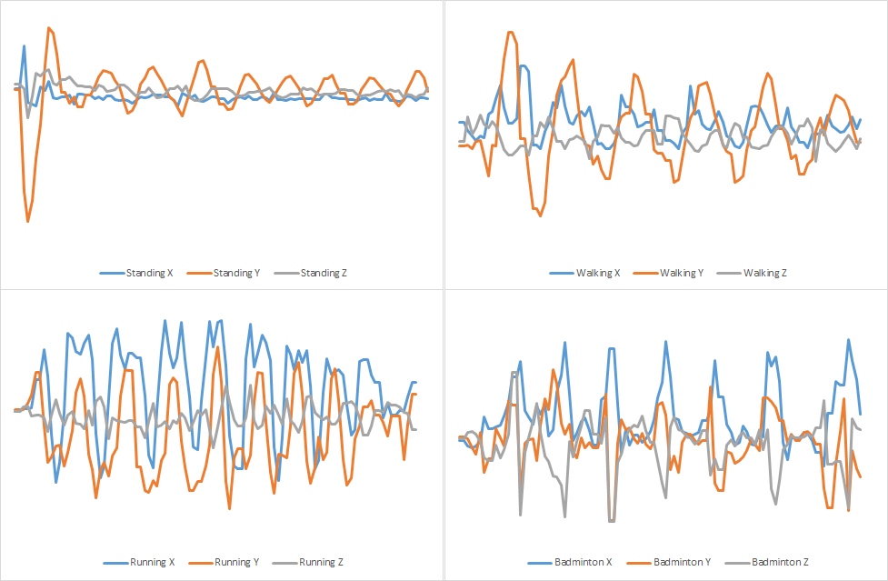
(a) Accelerometer MVMotion datasets

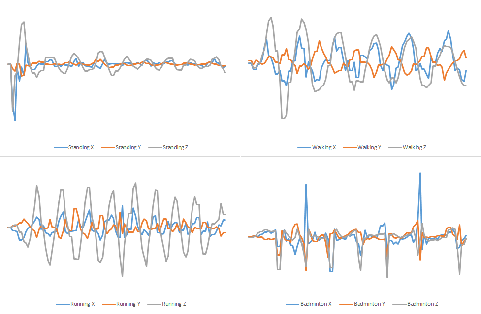
(b) Gyroscope MVMotion dataset

Figure 2: A list of the datasets in the multivariate time series archive. Number of instances is denoted by n, number of dimensions is denoted by d, length of series is denoted by m, and number of classes is denoted by c

. datasets n d m c AALTD_0 90 3 52 6 AALTD_1 90 3 52 6 AALTD_2 90 3 52 6 AALTD_3 90 3 52 6 AALTD_4 90 3 52 6 AALTD_5 90 3 52 6 AALTD_6 90 3 52 6 AALTD_7 90 3 52 6 ArabicDigit 6599 13 94 10 AWordLL 275 3 145 25 AWordT1 275 3 145 25 AWordUL 275 3 145 25 datasets n d m c CricketLeft 84 3 1198 12 CricketRight 84 3 1198 12 HandwritingA 150 3 153 26 HandwritingG 500 3 153 26 JapaneseVowels 270 12 30 9 MVMotionA 40 3 101 4 MVMotionAG 40 6 101 4 MVMotionG 40 3 101 4 PEMS 267 144 964 7 PenDigits 7494 2 9 10 UWaveGesture 120 3 316 8 VillarData 137 3 207 4

5 Multivariate Shapelet Transform

In this section we describe the three shapelet methods developed for the Multivariate Shapelet Transform. To illustrate the different methods, a series of figures have been created from a common dataset, demonstrating how all three methods find and extract different features, and how they calculate shapelet to series distance. The MVMotionA dataset is used in Figures 3, 4, and 5. In all three figures the left panel is the multivariate series shapelet extraction. In the middle left panel we demonstrate finding the minimum distance point whilst using the sliding window function. In Equation 4 we refer to this sliding window function as $sDist$. In the right panel, we show the exact comparison of the shapelet to the region in the multivariate series where both have been z-normalised.

5.1 Independent Shapelets

The first multivariate shapelet method is called Independent Shapelets. This algorithm finds single channel shapelets from any dimension. It then assesses the shapelets quality against the other series via sliding the shapelet along the same channel in the multivariate series. Once the $k$ best shapelets have been found, they are used to transform the original dataset. Using the same distance method, we can transform the multivariate dataset in a $k$ by $n$ matrix, where find the respective distance of the shapelets to each series.

The motivation for this method is that in some multivariate datasets the class defining feature may occur in only one channel, and it could even be independent of channel. The shape of the feature is the class identifier not its position or channel. We believe this method is most suited if you have multiple channels from different types of data recording where the dimensions are unrelated. One of the datasets we present MVMotionAG contains three channels of accelerometer data, and three channels of rotational(Gimbal) data. In some of the activity recognition the rotational data is completely independent of the movement information.

Figure 3: An example of extracting a single shapelet from a many dimensional series, and comparing it to a different series of the same dimension

.

(a) Shapelet extraction

(b) Shapelet matching

(c) Normalised distance

5.2 Multidimensional Dependent Shapelets

The second multivariate shapelet method is called Shapelet_D. This method extracts multi-dimensional shapelets, that are then compared to the other multivariate series, maintaining the phase across channels.

Once we have extracted a multi-dimension shapelet we slide each channel, simultaneously along each channel of all the other series, finding the minimum distance for each multivariate series with respect to the shapelet. Calculating a single distance for the multi-dimensional shapelet against all the other series means the algorithm behaves identically to the univariate Shapelet Transform, including calculating Information Gain, and transforming the data.

The main aspect of the Shapelet_D algorithm is that the minimum distance for a multivariate series and a multi-dimensional shapelet is that the position of best match is maintained across the channels. The motivation for this method is that for gesture recognition where a particular gesture is performed, all the channels (X,Y and Z) should have information about this event at the same point, but that the phase independence of shapelets means the information can be captured even though it can occur at any time interval.

Figure 4: An example of extracting a Shapelet_D from a many dimensional series, and comparing it to a different series

.

(a) Shapelet extraction

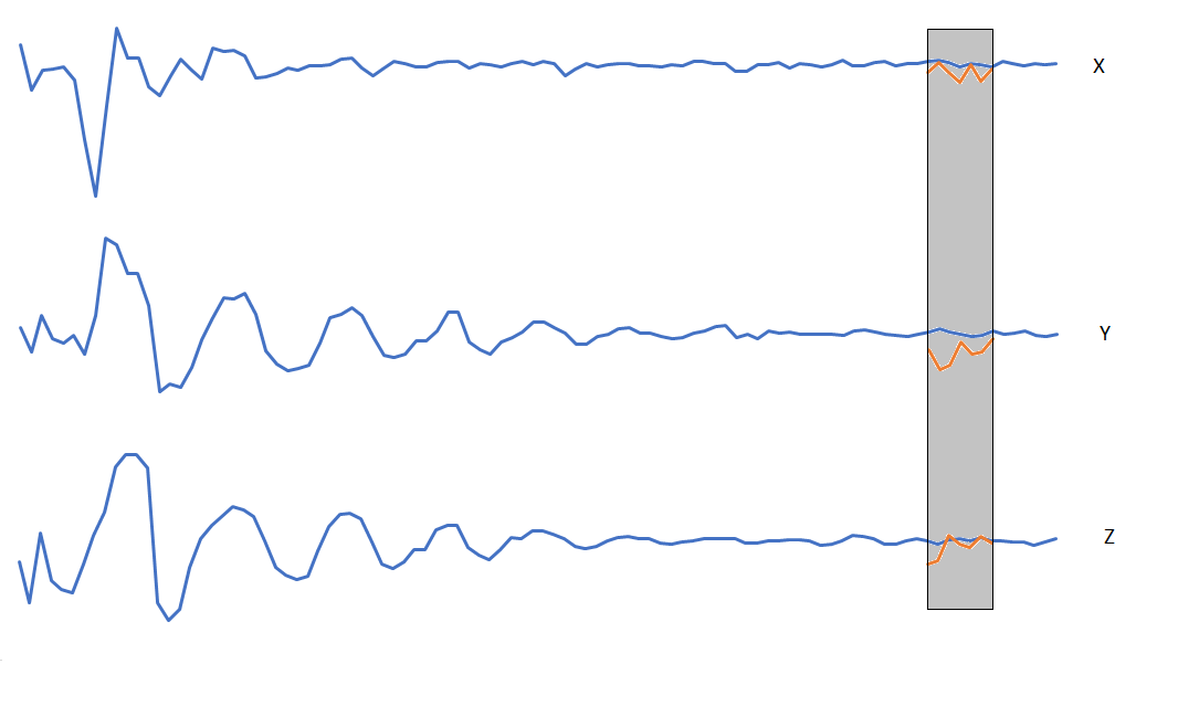
(b) Shapelet matching

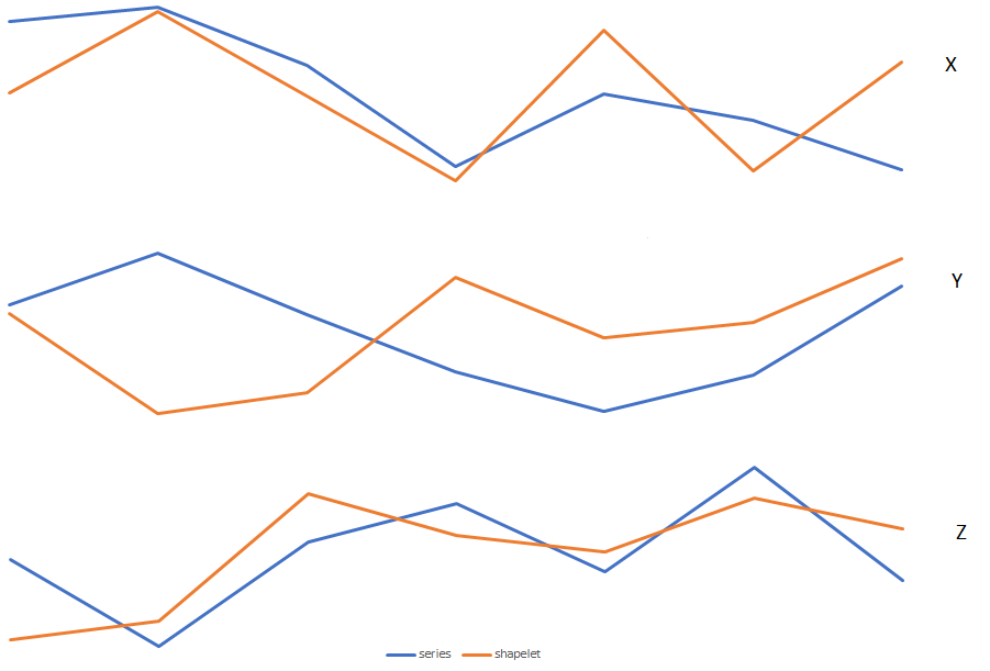
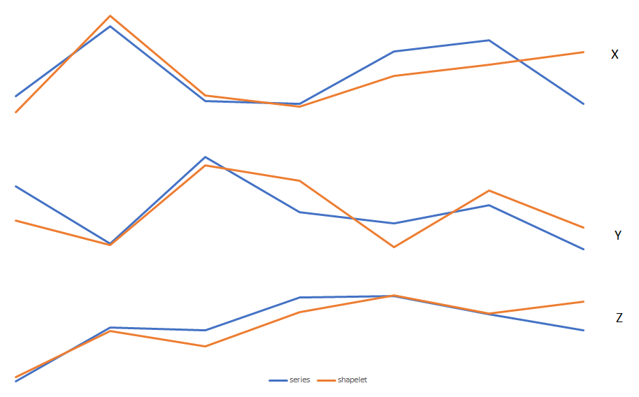
(c) Normalised distance

5.3 Multidimensional Independent Shapelets

The third multivariate shapelet method is called Shapelet_I. This method is similar to Shapelet_D which extracts multi-dimensional shapelets. These shapelets are then compared the other multivariate series. Each shapelet within the multi-dimensional shapelet finds the minimum distance to its respective channel independent of the other calculations. Shapelet_D could be considered a special case of the Shapelet_I algorithm where the best independent phase matches coincide to be the same.

The motivation for this method is that we believe whilst shapelet extracted is dependent on the features being in phase, the places where they occur in other series could be independent of one another.

Figure 5: We present an illustrative example of extracting a Shapelet_I from a many dimensional series, and comparing it to a different series

.

(a) Shapelet extraction

(b) Shapelet matching

(c) Normalised distance

6 Evaluation

The experimental setup follows the same approach outlined in [2]. We perform 100 fold resampling on the data. For each algorithm presented we have performed 2,400 experiments. The data presented in the tables are the mean average accuracy across the 100 folds. The critical difference diagrams are calculated from these mean averages. Resampling the datasets aids in identifying overall problem performance. When creating and processing these datasets from the literature and from our own data collection, the train and test splits are originally assigned randomly, thus on a single split the problem could be made arbitrarily hard. Some of the classifiers we use contain a random element, and so our experiments are all seeded to ensure reproducibility.

We initially present the results for the univariate methods for both, concatenation and dimensional ensembling. These algorithms are RotationForest(RotF), RandomForest (RandF), Support Vector Machine, Multi-Layer Perceptron and 1nearest neighbour with dynamic time warping. We use the notation _C to denote concatenation, and _E to denote ensembled across dimensions. These results show how concatenating dimensions into a single univariate series is superior to dimensional ensembling. However there are a few cases where the ensemble approach for DTW out performs concatenation. We believe given a cross-validated training approach to weight the respective ensemble dimensions, the ensembled method would be more robust. However the scale, and time requirements to cross-validate on these datasets is out of the scope of this work. The critical difference diagram Figure 6 shows there is no significant difference between DTW, the SVM, or random forest and rotation forest.

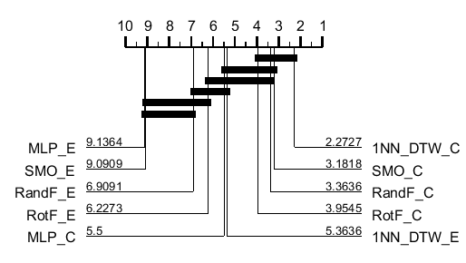
Figure 6: A critical difference diagram demonstrating the the effectiveness of the ensembling and concatenating approaches.

.

6.1 Shapelets

We present the results for our three multivariate shapelet methods on 17 datasets. Only 16 of the 22 datasets were able to complete full enumerations within a one week runtime limit on our HPC and the results from these are presented in Figure 7 in the second portion of the table we have also included a fixed one hour run time evaluation of the shapelet space for five additional datasets.

Initially we compare the shapelet methods across the 16 datasets over 100 fold resampling and show that Shapelet_D is not significantly worse than any of the multivariate DTW approaches, illustrated in 8a. We did multiple pairwise tests on each classifier, and found that Shapelet_D on a Wilcoxon signed rank test, and the student t-test is not significantly worse than any of the DTW approaches.

In previous work we have looked at heuristics for constraining the run time of the shapelet transform. A large portion of the univariate problems in the UEA-TSC archive are intractable to fully enumerate, by constraining the number of shapelets that are considered we can fix the run time of the algorithm. We constrained all the datasets to a one hour run time, where necessary. This meant we were able to evaluate an additional five datasets. From these results we find that Shapelet_D is still not significantly worse than any of the multivariate DTW approaches on 21 datasets all with 100 fold resampling, this is illustrated in 8b. We performed multiple pairwise tests and show that Shapelet_D with a constrained runtime of one hour is not significantly worse than any of the three DTW multivariate methods and is not significantly worse than a full enumeration.

The Shapelet_I method was significantly worse than the DTW_A and DTW_I but was not significantly worse than DTW_D on a Wilcoxon sign ranked test. Finally we found that the independent shapelet method was significantly worse than all multivariate DTW methods as well as Shapelet_D and was not significantly worse than Shapelet_I. Based on these findings Shapelet_D is an alternative approach to multivariate time series classification.

Figure 7:

. datasets SHAPELET_D INDEPENDENT SHAPELET_I DTW_A DTW_D DTW_I AALTD_0 0.646 (0.04) 0.583 (0.06) 0.569 (0.05) 0.664 (0.03) 0.681 (0.03) 0.649 (0.03) AALTD_1 0.792 (0.03) 0.725 (0.04) 0.744 (0.04) 0.805 (0.03) 0.804 (0.03) 0.809 (0.03) AALTD_2 0.608 (0.04) 0.529 (0.05) 0.557 (0.04) 0.667 (0.04) 0.675 (0.03) 0.671 (0.04) AALTD_3 0.661 (0.05) 0.61 (0.05) 0.656 (0.05) 0.684 (0.04) 0.68 (0.04) 0.683 (0.04) AALTD_4 0.624 (0.04) 0.576 (0.04) 0.619 (0.04) 0.657 (0.04) 0.667 (0.04) 0.667 (0.04) AALTD_5 0.767 (0.04) 0.735 (0.04) 0.735 (0.04) 0.789 (0.04) 0.797 (0.04) 0.777 (0.04) AALTD_6 0.617 (0.04) 0.542 (0.05) 0.461 (0.06) 0.654 (0.04) 0.671 (0.03) 0.639 (0.03) AALTD_7 0.796 (0.04) 0.739 (0.04) 0.746 (0.04) 0.791 (0.03) 0.784 (0.03) 0.791 (0.03) ArticularyWordLL 0.856 (0.02) 0.828 (0.02) 0.865 (0.02) 0.84 (0.02) 0.843 (0.02) 0.83 (0.02) ArticularyWordT1 0.923 (0.02) 0.901 (0.02) 0.894 (0.02) 0.921 (0.01) 0.924 (0.01) 0.908 (0.01) ArticularyWordUL 0.811 (0.03) 0.718 (0.03) 0.829 (0.03) 0.741 (0.02) 0.719 (0.02) 0.749 (0.02) HandwritingA 0.481 (0.03) 0.442 (0.03) 0.426 (0.03) 0.601 (0.03) 0.609 (0.02) 0.48 (0.02) JapaneseVowels 0.887 (0.02) 0.808 (0.03) 0.88 (0.02) 0.957 (0.01) 0.955 (0.01) 0.959 (0.01) MVMotionA 0.979 (0.02) 0.956 (0.02) 0.963 (0.03) 0.912 (0.05) 0.77 (0.04) 0.912 (0.05) MVMotionAG 0.984 (0.02) 0.953 (0.03) 0.961 (0.03) 0.999 (0) 0.951 (0.04) 0.999 (0) MVMotionG 0.936 (0.04) 0.939 (0.03) 0.933 (0.04) 0.996 (0.01) 0.917 (0.04) 0.996 (0.01) CricketLeft 0.92 (0.03) 0.819 (0.04) 0.869 (0.03) 0.927 (0.02) 0.933 (0.02) 0.887 (0.02) CricketRight 0.935 (0.02) 0.93 (0.03) 0.93 (0.03) 0.939 (0.03) 0.924 (0.03) 0.945 (0.03) HandwritingG 0.84 (0.01) 0.711 (0.1) 0.769 (0.11) 0.861 (0.05) 0.863 (0.05) 0.785 (0.04) UWaveGesture 0.898 (0.02) 0.868 (0.02) 0.862 (0.02) 0.919 (0.01) 0.925 (0.01) 0.909 (0.01) VillarData 0.969 (0.01) 0.978 (0.02) 0.981 (0.01) 0.965 (0.01) 0.957 (0.02) 0.969 (0.01)

Figure 8: Two critical difference diagrams demonstrating the effectiveness of the three shapelet transforms and the three multivariate DTW algorithms with full enumeration and one hour random shapelet selection

.

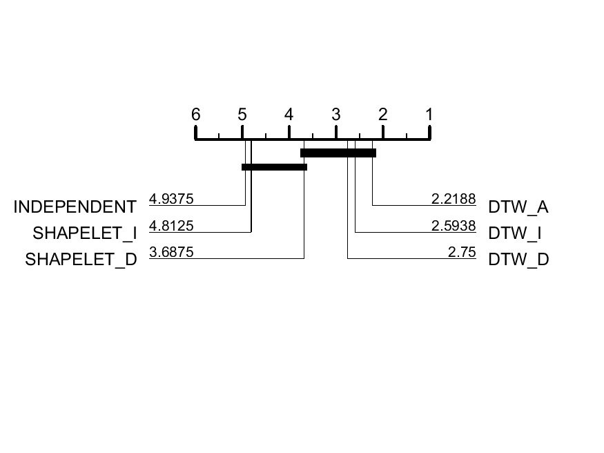
(a) Full enumeration with 17 datasets

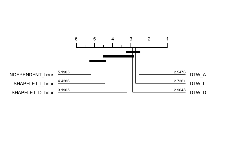
(b) One hour random shapelets with 21 datasets

7 Conclusion

In conclusion we have presented three new shapelet algorithms, one of which is not significantly worse than the current state-of-the-art in multivariate time series classification even when the search space is constrained. We have provided a unified set of datasets, under a common framework and file format. We provided some simple benchmarks of standard classifiers on these datasets to enable further research and comparison alongside the multivariate algorithms.

In future work we hope to be able to provide significantly better accuracy for shapelets, by assessing the way we measure the quality of multivariate shapelets, or by considering alternative distance measures.

We would also like to implement more of the multivariate algorithms from the literature under a common Java framework in WEKA to enable further analysis.

References

- [1] M. Shokoohi-Yekta, B. Hu, H. Jin, J. Wang, and E. Keogh, “Generalizing dtw to the multi-dimensional case requires an adaptive approach,” Data Mining and Knowledge Discovery, vol. 31, no. 1, pp. 1–31, 2017.
- [2] A. Bagnall, J. Lines, A. Bostrom, J. Large, and E. Keogh, “The great time series classification bake off: a review and experimental evaluation of recent algorithmic advance,” Data Mining and Knowledge Discovery, pp. 1–55, 2016.
- [3] J. Lines, L. Davis, J. Hills, and A. Bagnall, “A shapelet transform for time series classification,” in Proc. the 18th ACM SIGKDD International Conference on Knowledge Discovery and Data Mining, 2012.
- [4] A. Bostrom and A. Bagnall, “Binary shapelet transform for multiclass time series classification,” in Proc. 17th International Conference on Big Data Analytics and Knowledge Discovery (DAWAK), 2015.
- [5] J. Large, J. Lines, and A. Bagnall, “The Heterogeneous Ensembles of Standard Classification Algorithms (HESCA): the Whole is Greater than the Sum of its Parts,” 2017.
- [6] L. Ye and E. Keogh, “Time series shapelets: a novel technique that allows accurate, interpretable and fast classification,” Data Mining and Knowledge Discovery, vol. 22, no. 1-2, pp. 149–182, 2011.
- [7] J. Hills, J. Lines, E. Baranauskas, J. Mapp, and A. Bagnall, “Classification of time series by shapelet transformation,” Data Mining and Knowledge Discovery, vol. 28, no. 4, pp. 851–881, 2014.
- [8] I. Karlsson, P. Papapetrou, and H. Boström, “Forests of randomized shapelet trees,” in International Symposium on Statistical Learning and Data Sciences, pp. 126–136, Springer, 2015.
- [9] I. Karlsson, Order in the random forest. PhD thesis, Department of Computer and Systems Sciences, Stockholm University, 2017.
- [10] G. A. ten Holt, M. J. Reinders, and E. Hendriks, “Multi-dimensional dynamic time warping for gesture recognition,” in Thirteenth annual conference of the Advanced School for Computing and Imaging, vol. 300, 2007.
- [11] O. D. Lara and M. A. Labrador, “A survey on human activity recognition using wearable sensors.,” IEEE Communications Surveys and Tutorials, vol. 15, no. 3, pp. 1192–1209, 2013.
- [12] J. Liu, L. Zhong, J. Wickramasuriya, and V. Vasudevan, “uwave: Accelerometer-based personalized gesture recognition and its applications,” Pervasive and Mobile Computing, vol. 5, no. 6, pp. 657–675, 2009.
- [13] M. Ermes, J. Pärkkä, J. Mäntyjärvi, and I. Korhonen, “Detection of daily activities and sports with wearable sensors in controlled and uncontrolled conditions,” IEEE transactions on information technology in biomedicine, vol. 12, no. 1, pp. 20–26, 2008.
- [14] N. Kale, J. Lee, R. Lotfian, and R. Jafari, “Impact of sensor misplacement on dynamic time warping based human activity recognition using wearable computers,” in Proceedings of the conference on Wireless Health, p. 7, ACM, 2012.
- [15] M. H. Ko, G. West, S. Venkatesh, and M. Kumar, “Online context recognition in multisensor systems using dynamic time warping,” in Intelligent Sensors, Sensor Networks and Information Processing Conference, 2005. Proceedings of the 2005 International Conference on, pp. 283–288, IEEE, 2005.
- [16] J. Kela, P. Korpipää, J. Mäntyjärvi, S. Kallio, G. Savino, L. Jozzo, and S. Di Marca, “Accelerometer-based gesture control for a design environment,” Personal and Ubiquitous Computing, vol. 10, no. 5, pp. 285–299, 2006.
- [17] N. Gillian, B. Knapp, and S. O’Modhrain, “Recognition of multivariate temporal musical gestures using n-dimensional dynamic time warping.,” in NIME, pp. 337–342, 2011.
- [18] J. Tang and R. B. Dannenberg, “Extracting commands from gestures: Gesture spotting and recognition for real-time music performance,” in International Symposium on Computer Music Modeling and Retrieval, pp. 72–85, Springer, 2013.
- [19] K. Ø. Mikalsen, F. M. Bianchi, C. Soguero-Ruiz, S. O. Skrøvseth, R.-O. Lindsetmo, A. Revhaug, and R. Jenssen, “Learning similarities between irregularly sampled short multivariate time series from ehrs,” 2016.
- [20] T. Górecki and M. Łuczak, “Multivariate time series classification with parametric derivative dynamic time warping,” Expert Systems with Applications, vol. 42, no. 5, pp. 2305–2312, 2015.
- [21] A. Al-Jawad, M. R. Adame, M. Romanovas, M. Hobert, W. Maetzler, M. Traechtler, K. Moeller, and Y. Manoli, “Using multi-dimensional dynamic time warping for tug test instrumentation with inertial sensors,” in Multisensor Fusion and Integration for Intelligent Systems (MFI), 2012 IEEE Conference on, pp. 212–218, IEEE, 2012.
- [22] M. Bashir and J. Kempf, “Reduced dynamic time warping for handwriting recognition based on multidimensional time series of a novel pen device,” International Journal of Intelligent Systems and Technologies, WASET, vol. 3, no. 4, p. 194, 2008.
- [23] R. F. de Mello and I. Gondra, “Multi-dimensional dynamic time warping for image texture similarity,” in Brazilian Symposium on Artificial Intelligence, pp. 23–32, Springer, 2008.
- [24] Q. Zhu and E. Keogh, “Mother fugger: mining historical manuscripts with local color patches,” in Data Mining (ICDM), 2010 IEEE 10th International Conference on, pp. 699–708, IEEE, 2010.
- [25] C. A. Ratanamahatana and E. Keogh, “Three myths about dynamic time warping data mining,” in Proceedings of the 2005 SIAM International Conference on Data Mining, pp. 506–510, SIAM, 2005.
- [26] Y. Chen, B. Hu, E. Keogh, and G. E. Batista, “Dtw-d: time series semi-supervised learning from a single example,” in Proceedings of the 19th ACM SIGKDD international conference on Knowledge discovery and data mining, pp. 383–391, ACM, 2013.
- [27] O. P. Patri, R. Kannan, A. V. Panangadan, and V. K. Prasanna, “Multivariate time series classification using inter-leaved shapelets,” in NIPS 2015 Time Series Workshop, 2015.
- [28] I. Karlsson, P. Papapetrou, and L. Asker, “Multi-channel ecg classification using forests of randomized shapelet trees,” in Proceedings of the 8th ACM International Conference on PErvasive Technologies Related to Assistive Environments, p. 43, ACM, 2015.
- [29] J. Grabocka, M. Wistuba, and L. Schmidt-Thieme, “Fast classification of univariate and multivariate time series through shapelet discovery,” Fast classification of univariate and multivariate time series through shapelet discovery, vol. 49, pp. 429–454, 2016.
- [30] A. Bostrom, A. Bagnall, and J. Lines, “Evaluating improvements to the shapelet transform,”
- [31] j. Lines, s. Taylor, and A. Bagnall, “Time series classification with hive-cote: The hierarchical vote collective of transformation-based ensembles,” ACM Trans. Knowl. Discov. Data (under review), 2017.
- [32] M. Hall, E. Frank, G. Holmes, B. Pfahringer, P. Reutemann, and I. Witten, “The WEKA data mining software: An update,” SIGKDD Explorations, vol. 11, no. 1, pp. 10–18, 2009.
- [33] N. Hammami and M. Sellam, “Tree distribution classifier for automatic spoken arabic digit recognition,” in Internet Technology and Secured Transactions, 2009. ICITST 2009. International Conference for, pp. 1–4, IEEE, 2009.
- [34] M. Kudo, J. Toyama, and M. Shimbo, “Multidimensional curve classification using passing-through regions,” Pattern Recognition Letters, vol. 20, no. 11, pp. 1103–1111, 1999.
- [35] M. Cuturi, “Fast global alignment kernels,” in Proceedings of the 28th international conference on machine learning (ICML-11), pp. 929–936, 2011.
- [36] F. Alimoğlu and E. Alpaydin, “Combining multiple representations for pen-based handwritten digit recognition,” TURKISH JOURNAL OF ELECTRICAL ENGINEERING & COMPUTER SCIENCES, vol. 9, no. 1, pp. 1–12, 2001.
- [37] J. R. Villar, S. González, J. Sedano, C. Chira, and J. M. Trejo, “Human activity recognition and feature selection for stroke early diagnosis,” in International Conference on Hybrid Artificial Intelligence Systems, pp. 659–668, Springer, 2013.