Stellar Spin-Orbit Alignment for Kepler-9, a Multi-transiting Planetary system with Two Outer Planets Near 2:1 Resonance

Abstract

We present spectroscopic measurements of the Rossiter-McLaughlin effect for the planet b of Kepler-9 multi-transiting planet system. The resulting sky-projected spin-orbit angle is $\lambda=-13^{\circ}\pm 16^{\circ}$, which favors an aligned system and strongly disfavors highly misaligned, polar, and retrograde orbits. Including Kepler-9, there are now a total of 4 Rossiter-McLaughlin effect measurements for multiplanet systems, all of which are consistent with spin-orbit alignment.

1. Introduction

Hot Jupiters are frequently observed to have orbital angular momentum vectors that are strikingly misaligned with their stellar spin vectors. Stellar spin – planetary orbit misalignments are most frequently determined through spectroscopic measurements of the Rossiter-McLaughlin (R-M) effect (Rossiter, 1924; McLaughlin, 1924) during the planetary transit (Queloz et al., 2000), and have been recently reviewed by Winn & Fabrycky (2015).

Despite years of inquiry, the origin of the spin-orbit misalignments is still unclear. Dynamically active migration mechanisms (Notably, planet-planet scattering, Ford & Rasio 2008; Nagasawa et al. 2008; Lidov-Kozai Cycling with Tidal Friction, Wu & Murray 2003; Fabrycky & Tremaine 2007; Naoz et al. 2011; and secular chaos, Wu & Lithwick 2011), which violently deliver giant planets to short-period orbits, can naturally leave systems misaligned. In the framework of this hypothesis, the spin-orbital misalignments should represent a phenonmenon that is largely restricted to dynamically isolated hot Jupiters.

The possibility exists, however, that the spin-orbital misalignments can be excited via mechanisms that are unrelated to planet migration. These include chaotic star formation (Bate et al., 2010; Thies et al., 2011; Fielding et al., 2015) and evolution (Rogers et al., 2012), magnetic torques from host stars (Lai et al., 2011), and gravitational torques from distant companions (Tremaine, 1991; Batygin et al., 2011; Storch et al., 2014). In these scenarios, spin-orbit misalignments are expected to be observed not only among star-hot Jupiter pairs, but also among a broader class of planetary systems, notably those that have never experienced chaotic migration processes. This group is expected to include multiplanet systems, and especially multiplanet systems in mean motion resonance, MMR.

Table 1Radial velocity observations

Time [BJD]	Radial velocity [m/s]	Uncertainty [m/s]
2457959.810531	-3.00	4.93
2457959.825334	-5.54	5.15
2457959.839454	1.73	5.42
2457959.854084	13.12	5.60
2457959.868308	7.59	5.38
2457959.882834	-0.46	5.41
2457959.897139	21.06	4.67
2457959.911780	16.11	4.91
2457959.925715	23.18	4.70
2457959.940403	12.51	4.82
2457959.954766	7.50	4.58
2457959.968805	6.85	5.13
2457959.983041	-18.62	5.26
2457959.997405	-5.29	5.91
2457960.012115	-15.42	6.23
2457960.027092	-15.84	5.49
2457960.041143	-0.60	6.00
2457960.054904	-27.91	6.89
2457960.069117	0.10	8.19
2457960.084291	-29.22	8.59
2457960.098284	8.80	7.74

The R-M effect is much more easily measured when transits are frequent and deep. Therefore, as a practical consequence, although R-M observations of multiplanet systems play significant role in understanding planetary formation history, they are hard to make. They usually involve fainter stars, smaller transit depths, and/or less frequent transits, not to mention the scarcity of multiplanet systems in MMR. Although new methods (the $V\,{\rm sin}\,i$ method, Schlaufman 2010; Walkowicz & Basri 2013; Hirano et al. 2014; Morton & Winn 2014; Winn et al. 2017; the starspot-crossing method, Mazeh et al. 2015; Sanchis-Ojeda et al. 2011, 2012; Désert et al. 2011; Dai & Winn 2017, the starspot-variability method, Mazeh et al. 2015; the gravity-darkening method, Barnes 2009; Barnes et al. 2011; Szabó et al. 2011; Zhou & Huang 2013; the asteroseismic method, Gizon & Solanki 2003; Chaplin et al. 2013; Van Eylen et al. 2014; Huber et al. 2013; Benomar et al. 2014) have been developed to constrain the spin-orbit angles of multiplanet systems, as of this writing, only three robust R-M measurements exist (Kepler-89d, Hirano et al. 2012; Albrecht et al. 2013; WASP-47b, Sanchis-Ojeda et al. 2015; Kepler-25c, Albrecht et al. 2013).

In this light, Kepler-9 is particularly interesting. Kepler-9 was the first multiplanet system discovered using the transit method (Holman et al., 2010). It was also the first transiting system detected near 2:1 orbital mean motion resonance, which is believed to be the natural consequence of an evolutionary history that incorporates quiescent migration (Kley & Nelson, 2012). Whether this system has low spin-orbit angle or not, may provide a key zeroth-order test of origin scenarios of spin-orbit misalignments and competing migration paradigms for hot Jupiters. Kepler-9 b has very large planet-star size ratio of $R_{b}/R_{*}=0.0842\pm 0.0069$ (Twicken et al., 2016) – among the largest ratios yet detected in multiplanet systems. It thus offers a rare opportunity to carry out a spin-orbit angle measurement in a multiplanet system.

In this paper, we present a spin-orbit angle determination for the Kepler-9 multiplanet system that was obtained with spectroscopic R-M measurements. Our work provides additional empirical data that will further elucidate the origins of the spin-orbit misalignment distribution, and by extension, will shed light on the processes of planetary formation and evolution.

2. Observations and Data Reduction

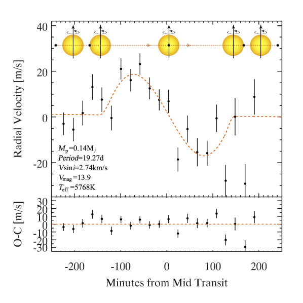
Figure 1.— Rossiter-McLaughlin effect observed in the Kepler-9 multiplanet system. Spectroscopic velocities spanning the transit of Kepler-9 b on the night of UT 2017 July 25 are plotted as dots with $1\,\sigma$ error bars. The orange dashed line correspond to the best-fit model which gives $\lambda=-13^{\circ}\pm 16^{\circ}$. The residuals with respect to the best-fit model are plotted in the lower panel.

In order to measure the R-M effect, we observed the Kepler-9b transit predicted by Wang et al. (2017) to occur on the night of UT 2017 July 25 using the High Resolution Spectrograph (HIRES; Vogt et al. 1994) on the Keck I $10\,{\rm m}$ Telescope atop Mauna Kea in Hawaii. Although the weather was generally clear, the seeing gradually degraded over the course of the night from 0$\farcs$9 to 2$\farcs$0. Observations were started $1.7\,{\rm hrs}$ before the predicted time of ingress, and finished $1.1\,{\rm hrs}$ after egress (when the star set below the pointing limitation of telescope). A fraction of light is picked off behind the slit and sent to an exposure meter that individual 20-minute exposures yielded a SNR between $29-45\,{\rm pixel^{-1}}$ at $5500{\rm\AA}$.

We obtained 21 spectra using a 0$\farcs$86 slit set by the B5 decker, which provides a spectral resolution, $R\sim 55,000$. The spectra were extracted with the reduction package of the California Planet Search team (Howard et al., 2010). For each of our observations, light from the star passes through an iodine cell positioned in front of the slit. This imprints a dense forest of ${\rm I_{2}}$ absorption lines that are used to model the wavelength and the spectral line spread function (SLSF) of the instrument. Spectroscopic Doppler shifts were modeled using the algorithm of Butler et al. (1996) and Marcy & Butler (1992). The Doppler analysis technique uses a template spectrum of the star obtained without the iodine cell and an extremely high-resolution, high SNR Fourier Transform Spectrograph (FTS) iodine spectrum to model the observations. The best fit model is driven by a Levenburg-Marquardt least squares algorithm and is a product of the template spectrum and the FTS ${\rm I_{2}}$ spectrum that is then convolved with a description Valenti et al. (1995) of the SLSF. The free parameters in the model include the wavelength zero point, the dispersion, the Doppler shift and a multi-Gaussian fit to the line broadening function. At the SNR of our Kepler-9 observations, the Doppler shift was modeled with a precision of about $6\,{\rm m\,s^{-1}}$. The resulting RVs and their uncertainties are presented in Table 1, and shown in Figure 1.

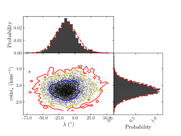
Figure 2.— Posterior probability distribution of $\lambda$ and $v\sin i_{\star}$ from the MCMC simulation of the Kepler-9 observations. The contours show the 1, 2, and 3 $\sigma$ confidence regions (in blue, yellow, and red, respectively). We have marginalized over $\lambda$ and $v\sin i_{\star}$ and have fit them with Gaussians (in red). This plot indicates that the distribution is Gaussian, which suggests that $\lambda$ and $v\sin i_{\star}$ are not strongly correlated with each other.

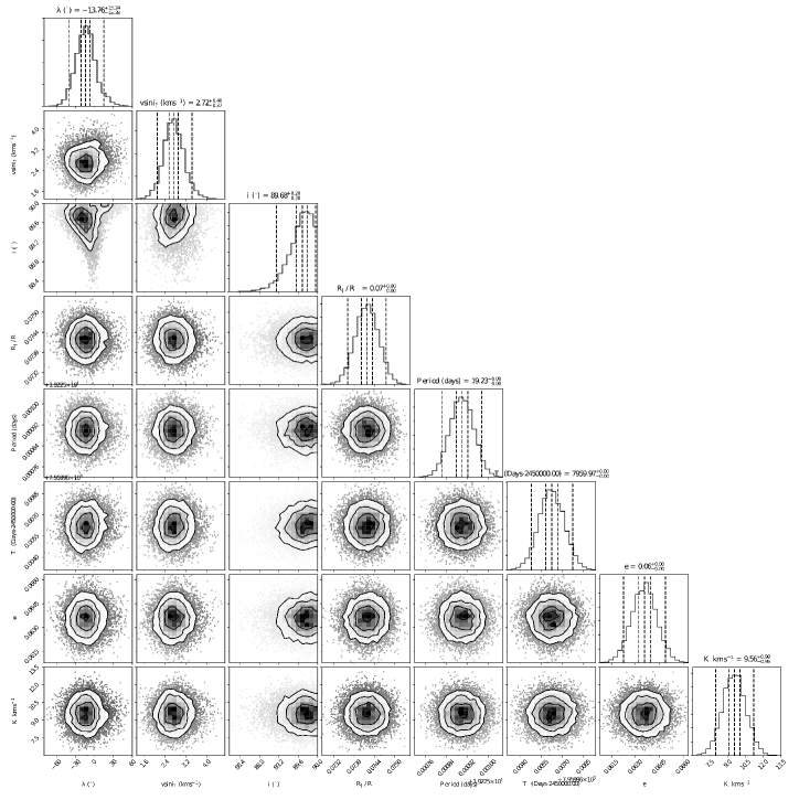
Figure 3.— Corner posterior probability distribution plots of the MCMC fitting parameters for the R-M anomaly fit to the Kepler-9 radial velocity data. The histograms along the diagonal show the marginalized posterior distribution for each fitting parameter. The $1\sigma$ and $2\sigma$ credibility intervals are marked by vertical dashed lines.

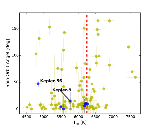
Figure 4.— Spin-orbit angle as a function of stellar effective temperature. Yellow dots are single-planet systems. Blue dots are multi-planet systems. The red dashed line at 6250K indicates the location of the Kraft Break (Kraft, 1967).

3. Analysis of the Observations

3.1. Independent Determination of the Projected Stellar Rotational Velocity

We analyzed the iodine-free template observations to determine the stellar parameters and abundances using the spectral fitting procedure and line list of Brewer et al. (2016). The procedure has been shown to retrieve gravities consistent with those from asteroseismology to within 0.05 dex (Brewer et al., 2015) in addition to accurate temperatures, precise abundances for a range of elements, and projected rotational velocities ($v\sin i$).

We first fit for the global stellar parameters, including effective temperature ($T_{\mathrm{eff}}$), surface gravity ($\log g$), metallicity ([Fe/H]), macroturbulence ($v_{mac}$), and the abundances of the alpha elements calcium, silicon, and titanium. The initial guess for $T_{\mathrm{eff}}$ is set using the B-V color and the remaining parameters are set to solar values except for $v\sin i$, which is set to zero. We perturb the temperature by $\pm 100$ K and re-fit, using the ${\chi}^{2}$-weighted average of the three fits for the input to our next step. We then fix the global parameters, and solve for the abundances of 15 elements (C, N, O, Na, Mg, Al, Si, Ca, Ti, V, Cr, Mn, Fe, Ni, and Y). With this new abundance pattern, we then iterate the entire procedure once. Finally, we set the macroturbulence to using the $v_{mac}/T_{\mathrm{eff}}$ relation derived in Brewer et al. (2016) and fit for $v\sin i$. The combined uncertainties in macroturbulence and projected rotational velocity are 0.7 km/s. Assuming equal contributions from both $v_{mac}$ and $v\sin i$ gives uncertainties of 0.5 km/s for each. Our extensive line list and differential solar analysis leads to very low statistical uncertainties in our abundances. However, model simplifications and uncertainties in the solar abundances lead to additional uncertainty in the accuracy of our abundances. We add 0.03 dex in quadrature to the abundance uncertainties to account for the accuracy when comparing to other studies.

Our results for $T_{\mathrm{eff}}=5768\pm 25{\mathrm{K}}$, $\log g=4.50\pm 0.05$, ${\mathrm{[Fe/H]}}=0.035\pm 0.01$, and $v\sin i=2.96\pm 0.5~{}{\mathrm{km\,s^{-1}}}$ are, in general, consistent with recent determinations in the literature (Petigura et al., 2017; Huber et al., 2014; Buchhave et al., 2012). There is small difference in [Fe/H] as compared to Buchhave et al. (2012) at about the two sigma level.

3.2. Determination of the Projected Stellar Obliquity

We used the Exoplanetary Orbital Simulation and Analysis Model (ExOSAM; see Addison et al., 2013, 2014, 2016) to determine the best-fit $\lambda$ value for Kepler-9 from the R-M effect measurements. ExOSAM utilizes a Metropolis-Hastings Markov Chain Monte Carlo (MCMC) algorithm to derive accurate posterior probability distributions of $\lambda$ and $v\sin i_{\star}$ and to optimize their fit to the RV data, largely following the procedure described in Addison et al. (2016). The optimal solutions for $\lambda$ and $v\sin i_{\star}$, as well as their $1\sigma$ uncertainties, are calculated from the mean and the standard deviation of all the accepted MCMC iterations, respectively.

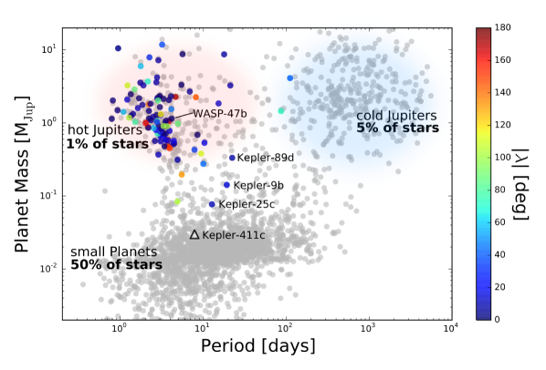
Figure 5.— An up-to-date mass-period diagram delineating the current extrasolar planetary catalog. Objects with Rossiter-Mclaughlin measurements (including Doppler Tomography measurements) drawn from the TEPCat (Southworth, 2011), are shown as solid points color-coded by the measured projected spin-orbit angles, while objects without Rossiter-Mclaughlin measurements are depicted as gray transparent dots. Almost all the existing measurements are for hot Jupiters, which are intrinsically rare but readily studied. These observations have revealed a wide range of configurations of spin-orbit angles. In this work, we have expanding the list of measurements to include a member of the Kepler-9 multi-planet system, thereby probing a representative of the most populous known group of extrasolar planets.

Table 2 lists the prior value, the $1\sigma$ uncertainty, and the prior type of each parameter used in the ExOSAM model. The results of the MCMC analysis and the best-fit values for $\lambda$ and $v\sin i_{\star}$ are also given in Table 2. For this analysis, we ran 10 independent MCMC walkers for 50,000 accepted iterations to obtain good mixing and convergence in each of the MCMC chains.

We fixed the argument of periastron ($\omega$) given the low orbital eccentricity as well as the lack of out-of-transit RV data. We accounted for the uncertainties on $R_{\star}$ and $R_{P}$ by imposing a Gaussian prior on the planet-to-star radius ratio ($R_{P}/R_{\star}$) as well as a Gaussian prior on the stellar radius ($R_{\star}$) to account for the uncertainty in the length of the transit. Gaussian priors were imposed on the quadratic limb darkening coefficients ($q_{1}$) and ($q_{2}$) based on interpolated values from look-up tables in Claret & Bloemen (2011). We incorporated the uncertainties on the mid-transit epoch ($T_{0}$), the orbital period ($P$), orbital inclination angle ($I$), orbital eccentricity ($e$), stellar macro-turbulence ($v_{\mathrm{mac}}$), RV zero offset ($V_{0}$), and the stellar velocity semi amplitude ($K$) into our model using Gaussian priors from the literature. For $\lambda$, we used a uniform prior on the interval $-90^{\circ}$ to $90^{\circ}$. The Gaussian prior we placed on ${v\sin i_{\star}}$ was determined using the iodine-free spectrum template observations we obtained for Kepler-9 on the night of the transit.

Figure 1 shows the modeled Rossiter–McLaughlin anomaly with the observed velocities overplotted. The Rossiter–McLaughlin effect is seen as a positive anomaly between $\sim\!150$ minutes prior to mid-transit and mid-transit and then as a negative anomaly between mid-transit and $\sim\!150$ minutes after mid-transit. This indicates that Kepler-9b first transits across the blue-shifted hemisphere during ingress and then across the red-shifted hemisphere during egress, producing a nearly symmetrical velocity anomaly. Therefore, the orbit of Kepler-9b is likely to be nearly in projected alignment with the spin axis of its host star (that is, the system is likely in “spin–orbit alignment”). Figure 1 does reveal an increase in RV scatter around egress from poorer ($\sim 1.5^{\texttt{"}}$) seeing conditions.

The posterior probability distributions of $\lambda$ and $v\sin i_{\star}$, are shown in Figure 2. The $1\sigma$, $2\sigma$, and $3\sigma$ confidence contours are plotted, along with normalized density functions marginalized over $\lambda$ and $v\sin i_{\star}$ with fitted Gaussians. The distributions, marginalized over $\lambda$ and $v\sin i_{\star}$, adhere fairly well to a normal distribution, and appear to not be strongly correlated with each other. To check if $\lambda$ or $v\sin i_{\star}$ are strongly correlated with any of the other model parameters and to reveal covariances, we have produced a series of corner posterior probability distribution plots, which are shown in 3.

[b] Input Parameter Prior Prior Type Results Mid-transit epoch (2450000-HJD), $T_{0}$ $7959.9661\pm 0.0009$^a Gaussian $7959.9661\pm 0.0009$ Orbital period (days), $P$ $19.225900\pm 0.000046$^a Gaussian $19.225900\pm 0.000046$ Orbital inclination, $I$ $89.74^{\circ}\pm 0.70^{\circ}$^b Gaussian $89.64^{\circ}\pm 0.26^{\circ}$ Planet-to-star radius ratio, $R_{P}/R_{\star}$ $0.074186^{+0.00022}_{-0.000348}$^b,c Gaussian $0.074181\pm 0.000351$ Orbital eccentricity, $e$ $0.0636\pm 0.0008$^a Gaussian $0.0636\pm 0.0008$ Argument of periastron, $\omega$ $357.03^{\circ}\pm 0.44^{\circ}$^a Fixed^d – Stellar mass, $M_{\star}$ $1.034^{+0.058}_{-0.080}$ $M_{\odot}$^b Fixed – Stellar radius, $R_{\star}$ $0.956^{+0.147}_{-0.053}$ $R_{\odot}$^b Gaussian $0.982\pm 0.068$ $R_{\odot}$ Planet mass, $M_{P}$ $0.1384\pm 0.0015$ $M_{J}$^a Fixed^d – Planet radius, $R_{P}$ $0.6905^{+0.1071}_{-0.0375}$ $R_{J}$^{b, e} Fixed – Impact parameter, $b$ $0.143\pm 0.022$^f – – Stellar velocity semi-amplitude, $K$ $9.55\pm 0.98$  m s^-1a Gaussian $9.56\pm 0.98$  m s^-1 Stellar micro-turbulence, $\xi_{t}$ N/A Fixed – Stellar macro-turbulence, $v_{\mathrm{mac}}$ $3.47\pm 0.5$  km s^-1g Gaussian $3.46\pm 0.69$  km s^-1 Stellar limb-darkening coefficient, $q_{1}$ $0.4699\pm 0.0463$^h Gaussian $0.4699\pm 0.0462$ Stellar limb-darkening coefficient, $q_{2}$ $0.2507\pm 0.0440$^h Gaussian $0.2506\pm 0.0439$ RV zero offset, $V_{0}$ $0.0\pm 5.0$  m s^-1 Gaussian $0.5\pm 1.4$  m s^-1 Projected obliquity angle, $\lambda$ $[-90^{\circ}\textendash\,90^{\circ}]$ Uniform $-13^{\circ}\pm 16^{\circ}$ Projected stellar rotation velocity, ${v\sin i_{\star}}$ $2.96\pm 0.50$  km s^-1g Gaussian $2.74\pm 0.40$  km s^-1 a Prior values determined through our dynamical simulations of transit timing variations derived from the full Kepler data set and from a photometric transit observation of Kepler-9 on UT 2016 September 1. b Prior values given by the NASA Exoplanet Archive in the cumulative table of planet candidates and used in the MCMC. c In cases where the prior uncertainty is asymmetric, for simplicity, we use a symmetric Gaussian prior with the prior width set to the larger uncertainty value in MCMC. d Prior fixed to allow convergence of MCMC chains. e Planet radius given here for informative purposes and determined from planet-to-star radius ratio prior. f Parameter and value given for informative purposes. g Priors determined from Kepler-9 spectrum template observations. h Limb darkening coefficients interpolated from the look-up tables in Claret & Bloemen (2011).

Table 2System Parameters, Priors, and Results for Kepler-9

4. Discussion

Kepler-9 has a mass and an effective temperature that are very close to the solar values. For a number of years, as the first planetary Rossiter-McLaughlin measurements were accumulating in the literature, there was evidence that planets transiting relatively low-mass ($M\lesssim 1.1M_{\odot}$), low temperature ($T\lesssim 6200K$) stars tend to have low-obliquity orbits, with the converse being true of planets orbiting higher-mass stars. Early data arguments for this picture can be found in Schlaufman (2010), Winn et al. (2010), and Albrecht et al. (2012).

The picture is no longer so clear-cut. The number of planet-star pairs with spin-orbit measurements has been increasing steadily, and the total number of systems with measurements is of order $N\sim 120$. Figure 4 gathers the projected obliquities obtained to date, showing that while there is still an apparent statistical tendency for low-temperature stars to favor aligned orbits, the correlation has weakened substantially. As pointed out recently by Dai & Winn (2017), however, among planets with $a(1-e)\lesssim 6R_{\star}$ orbiting low-mass stars, low-obliquity is still the rule. A similar pattern was also shown in Triaud (2017). This dichotomy hints at the potential importance of star-disk interactions for driving alignment in low-mass systems that had $\sim 10^{3}$ gauss magnetic fields during the T-Tauri stage (Dawson, 2014; Spalding & Batygin, 2015), and hints as well that star-planet tides may also be playing a coplanarizing role (Winn et al., 2010; Anderson et al., 2015).

Kepler-9b, with its long orbital period and its resonant lock to an exterior companion would likely be less prone to either evolutionary process, and one would likely retain any primordial spin-orbit misalignment. Therefore, the observed co-planarity may point to an early history in which migration and accretion occurred in isolation and with relatively little disturbance.

Finally, it is useful to note that spin-obit alignment measurements are only beginning to probe the truly representative populations of planets. As indicated by the summary diagram shown in Figure 5, the hot Jupiters (which accompany $<1$% of stars (Batalha et al., 2013)) have had their orbital obliquities sampled very heavily, but the overwhelmingly more common super-Earths and sub-Neptunes (as well as the population of longer-period Jovian planets) have as-yet barely been touched. The Kepler-9 planets lie in the sparsely populated transition region with $10\,{\rm d}\lesssim P\lesssim 100\,{\rm d}$, and $30\,{M_{\oplus}}\lesssim P\lesssim 100\,{M_{\oplus}}$. Forthcoming measurements – such as those planned for Kepler 411-c – will probe the great bulk of the distribution, and should clarify what happens when the planet formation process follows the apparent path of least resistance.

References

- Albrecht et al. (2012) Albrecht, S., Winn, J. N., Johnson, J. A., et al. 2012, ApJ, 757, 18
- Albrecht et al. (2013) Albrecht, S., Winn, J. N., Marcy, G. W., et al. 2013, ApJ, 771, 11
- Anderson et al. (2015) Anderson, D. R., Triaud, A. H. M. J., Turner, O. D., et al. 2015, ApJ, 800, L9
- Addison et al. (2013) Addison, B. C., Tinney, C. G., Wright, D. J., et al. 2013, ApJ, 774, 9
- Addison et al. (2014) Addison, B. C., Tinney, C. G., Wright, D. J., & Bayliss, D. 2014, ApJ, 792, 112
- Addison et al. (2016) Addison, B. C., Tinney, C. G., Wright, D. J., & Bayliss, D. 2016, ApJ, 823, 29
- Barnes (2009) Barnes, J. W. 2009, ApJ, 705, 683
- Barnes et al. (2011) Barnes, J. W., Linscott, E., & Shporer, A. 2011, ApJS, 197, 10
- Batalha et al. (2013) Batalha, N. M., Rowe, J. F., Bryson, S. T., et al. 2013, ApJS, 204, 24
- Bate et al. (2010) Bate, M. R., Lodato, G., & Pringle, J. E. 2010, MNRAS, 401, 1505
- Batygin et al. (2011) Batygin, K., Morbidelli, A., & Tsiganis, K. 2011, A&A, 533, A7
- Benomar et al. (2014) Benomar, O., Masuda, K., Shibahashi, H., & Suto, Y. 2014, PASJ, 66, 94
- Brewer et al. (2015) Brewer, J. M., Fischer, D. A., Basu, S., Valenti, J. A., & Piskunov, N. 2015, ApJ, 805, 126
- Brewer et al. (2016) Brewer, J. M., Fischer, D. A., Valenti, J. A., & Piskunov, N. 2016, ApJS, 225, 32
- Buchhave et al. (2012) Buchhave, L. A., Latham, D. W., Johansen, A., et al. 2012, Nature, 486, 375
- Butler et al. (1996) Butler, R. P., Marcy, G. W., Williams, E., et al. 1996, PASP, 108, 500
- Campante et al. (2016) Campante, T. L., Lund, M. N., Kuszlewicz, J. S., et al. 2016, ApJ, 819, 85
- Chaplin et al. (2013) Chaplin, W. J., Sanchis-Ojeda, R., Campante, T. L., et al. 2013, ApJ, 766, 101
- Claret & Bloemen (2011) Claret, A. & Bloemen, S. 2011, A&A, 529, 75
- Dai & Winn (2017) Dai, F., & Winn, J. N. 2017, AJ, 153, 205
- Dawson (2014) Dawson, R. I. 2014, ApJ, 790, L31
- Désert et al. (2011) Désert, J.-M., Charbonneau, D., Demory, B.-O., et al. 2011, ApJS, 197, 14
- Fabrycky & Tremaine (2007) Fabrycky, D., & Tremaine, S. 2007, ApJ, 669, 1298
- Fielding et al. (2015) Fielding, D. B., McKee, C. F., Socrates, A., Cunningham, A. J., & Klein, R. I. 2015, MNRAS, 450, 3306
- Ford & Rasio (2008) Ford, E. B., & Rasio, F. A. 2008, ApJ, 686, 621
- Gizon & Solanki (2003) Gizon, L., & Solanki, S. K. 2003, ApJ, 589, 1009
- Hébrard et al. (2008) Hébrard, G., Bouchy, F., Pont, F., et al. 2008, A&A, 488, 763
- Hirano et al. (2012) Hirano, T., Narita, N., Sato, B., et al. 2012, ApJ, 759, L36
- Hirano et al. (2014) Hirano, T., Sanchis-Ojeda, R., Takeda, Y., et al. 2014, ApJ, 783, 9
- Holman et al. (2010) Holman, M. J., Fabrycky, D. C., Ragozzine, D., et al. 2010, Science, 330, 51
- Howard et al. (2010) Howard, A. W., Johnson, J. A., Marcy, G. W., et al. 2010, ApJ, 721, 1467
- Huber et al. (2014) Huber, D., Silva Aguirre, V., Matthews, J. M., et al. 2014, ApJS, 211, 2
- Huber et al. (2013) Huber, D., Carter, J. A., Barbieri, M., et al. 2013, Science, 342, 331
- Kley & Nelson (2012) Kley, W., & Nelson, R. P. 2012, ARA&A, 50, 211
- Kraft (1967) Kraft, R. P. 1967, ApJ, 150, 551
- Lai et al. (2011) Lai, D., Foucart, F., & Lin, D. N. C. 2011, MNRAS, 412, 2790
- Marcy & Butler (1992) Marcy, G. W., & Butler, R. P. 1992, PASP, 104, 270
- Mazeh et al. (2015) Mazeh, T., Holczer, T., & Shporer, A. 2015a, ApJ, 800, 142
- Mazeh et al. (2015) Mazeh, T., Perets, H. B., McQuillan, A., & Goldstein, E. S. 2015b, ApJ, 801, 3
- McLaughlin (1924) McLaughlin, D. B. 1924, ApJ, 60,
- Morton & Winn (2014) Morton, T. D., & Winn, J. N. 2014, ApJ, 796, 47
- Nagasawa et al. (2008) Nagasawa, M., Ida, S., & Bessho, T. 2008, ApJ, 678, 498
- Naoz et al. (2011) Naoz, S., Farr, W. M., Lithwick, Y., Rasio, F. A., & Teyssandier, J. 2011, Nature, 473, 187
- Petigura et al. (2017) Petigura, E. A., Howard, A. W., Marcy, G. W., et al. 2017, AJ, 154, 107
- Queloz et al. (2000) Queloz, D., Eggenberger, A., Mayor, M., et al. 2000, A&A, 359, L13
- Rogers et al. (2012) Rogers, T. M., Lin, D. N. C., & Lau, H. H. B. 2012, ApJ, 758, L6
- Rossiter (1924) Rossiter, R. A. 1924, ApJ, 60,
- Sanchis-Ojeda et al. (2011) Sanchis-Ojeda, R., Winn, J. N., Holman, M. J., et al. 2011, ApJ, 733, 127
- Sanchis-Ojeda et al. (2012) Sanchis-Ojeda, R., Fabrycky, D. C., Winn, J. N., et al. 2012, Nature, 487, 449
- Sanchis-Ojeda et al. (2015) Sanchis-Ojeda, R., Winn, J. N., Dai, F., et al. 2015, ApJ, 812, L11
- Schlaufman (2010) Schlaufman, K. C. 2010, ApJ, 719, 602
- Southworth (2011) Southworth, J. 2011, MNRAS, 417, 2166
- Spalding & Batygin (2015) Spalding, C., & Batygin, K. 2015, ApJ, 811, 82
- Storch et al. (2014) Storch, N. I., Anderson, K. R., & Lai, D. 2014, Science, 345, 1317
- Szabó et al. (2011) Szabó, G. M., Szabó, R., Benkő, J. M., et al. 2011, ApJ, 736, L4
- Thies et al. (2011) Thies, I., Kroupa, P., Goodwin, S. P., Stamatellos, D., & Whitworth, A. P. 2011, MNRAS, 417, 1817
- Triaud (2017) Triaud, A. H. M. J. 2017, arXiv:1709.06376
- Tremaine (1991) Tremaine, S. 1991, Icarus, 89, 85
- Twicken et al. (2016) Twicken, J. D., Jenkins, J. M., Seader, S. E., et al. 2016, AJ, 152, 158
- Valenti et al. (1995) Valenti, J. A., Butler, R. P., & Marcy, G. W. 1995, PASP, 107, 966
- Van Eylen et al. (2014) Van Eylen, V., Lund, M. N., Silva Aguirre, V., et al. 2014, ApJ, 782, 14
- Vogt et al. (1994) Vogt, S. S., Allen, S. L., Bigelow, B. C., et al. 1994, Proc. SPIE, 2198, 362
- Walkowicz & Basri (2013) Walkowicz, L. M., & Basri, G. S. 2013, MNRAS, 436, 1883
- Wang et al. (2017) Wang, S., Wu, D.-H., Addison, B., et al. 2017, Submitted.
- Winn et al. (2010) Winn, J. N., Fabrycky, D., Albrecht, S., & Johnson, J. A. 2010, ApJ, 718, L145
- Winn & Fabrycky (2015) Winn, J. N., & Fabrycky, D. C. 2015, ARA&A, 53, 409
- Winn et al. (2017) Winn, J. N., Petigura, E. A., Morton, T. D., et al. 2017, arXiv:1710.04530
- Wu & Murray (2003) Wu, Y., & Murray, N. 2003, ApJ, 589, 605
- Wu & Lithwick (2011) Wu, Y., & Lithwick, Y. 2011, ApJ, 735, 109
- Zhou & Huang (2013) Zhou, G., & Huang, C. X. 2013, ApJ, 776, L35