A characterization of the Non-Degenerate Source Condition in Super-Resolution

Vincent Duval111INRIA, Mokaplan 222CEREMADE, Université Paris-Dauphine, Place du Marechal De Lattre De Tassigny, 75775 PARIS CEDEX 16, FRANCE.
Abstract

In a recent article, Schiebinger et al. provided sufficient conditions for the noiseless recovery of a signal made of M𝑀M Dirac masses given 2M+12𝑀12M+1 observations of, e.g. , its convolution with a Gaussian filter, using the Basis Pursuit for measures. In the present work, we show that a variant of their criterion provides a necessary and sufficient condition for the Non-Degenerate Source Condition (NDSC) which was introduced by Duval and Peyré to ensure support stability in super-resolution. We provide sufficient conditions which, for instance, hold unconditionally for the Laplace kernel provided one has at least 2M2𝑀2M measurements. For the Gaussian filter, we show that those conditions are fulfilled in two very different configurations: samples which approximate the uniform Lebesgue measure or, more surprisingly, samples which are all confined in a sufficiently small interval.

Keywords:

Super-resolution; 1superscript1\ell^{1} norm; Total Variation minimization; LASSO for measures; T-Systems

AMS subject classifications:

90C25, 68U10

1 Introduction

Super-resolution imaging, or observing small structures below the diffraction limit, is a fundamental problem in optical science, concerning applications such as microscopy [32], astronomy [37], medical imaging [22]. It is also of great importance in radar sensing [34] and geophysics [30]. While practical methods have made tremendous progress, the mathematical understanding of that problem is still limited. With the seminal works on sparse super-resolution [11, 5, 7] and the simultaneous emergence of “off-the-grid” methods for line spectral estimation [3, 45], several theoretical advances have been made in the recovery of sparse signals in a continuous domain.

Typically, given a domain X𝑋X\subseteq\mathbb{R}, one wants to recover the signal

m0=def.i=1Maiδxisuperscriptdef.subscript𝑚0superscriptsubscript𝑖1𝑀subscript𝑎𝑖subscript𝛿subscript𝑥𝑖\displaystyle m_{0}\stackrel{{\scriptstyle\mbox{\tiny def.}}}{{=}}\sum_{i=1}^{M}a_{i}\delta_{x_{i}} (1)

where {xi}i=1MXsuperscriptsubscriptsubscript𝑥𝑖𝑖1𝑀𝑋\{x_{i}\}_{i=1}^{M}\subset X are spikes locations and {ai}i=1Msuperscriptsubscriptsubscript𝑎𝑖𝑖1𝑀\{a_{i}\}_{i=1}^{M}\subset\mathbb{C} are their amplitudes, but one only has access to the observation

y=i=1Maiφ(xi)+w,𝑦superscriptsubscript𝑖1𝑀subscript𝑎𝑖𝜑subscript𝑥𝑖𝑤\displaystyle y=\sum_{i=1}^{M}a_{i}\varphi(x_{i})+w, (2)

where φ(x)𝜑𝑥\varphi(x)\in\mathcal{H} is the impulse response, or point spread function (in a generalized sense), \mathcal{H} is a Hilbert space, and w𝑤w is some additive noise. For instance, one may consider X=[0,1]𝑋01X=[0,1], =Ksuperscript𝐾\mathcal{H}=\mathbb{C}^{K}, and let φ(x)=(cjk(m))1kK𝜑𝑥subscriptsubscript𝑐subscript𝑗𝑘𝑚1𝑘𝐾\varphi(x)=(c_{j_{k}}(m))_{1\leqslant k\leqslant K} be a vector containing the Fourier coefficients of δxsubscript𝛿𝑥\delta_{x} for K𝐾K prescribed frequencies (see [7]). Alternatively, one may choose =L2()superscriptL2\mathcal{H}=\text{L}^{2}(\mathbb{R}) and φ(x)=ψ~(x)\varphi(x)=\tilde{\psi}(\cdot-x) is the impulse response of a linear translation invariant filter [46]. A more realistic setting is to consider that the convolution has been sampled, which can be handled using the more general choice

φ(x):sψ(x,s)and=L2(S,PS),:𝜑𝑥formulae-sequencemaps-to𝑠𝜓𝑥𝑠andsuperscriptL2𝑆subscript𝑃𝑆\displaystyle\varphi(x):{s}\mapsto\psi(x,{s})\quad\text{and}\quad\mathcal{H}=\text{L}^{2}(S,P_{S}), (3)

where ψ𝜓\psi encodes the impulse response (e.g. ψ(x,s)=ψ~(sx)𝜓𝑥𝑠~𝜓𝑠𝑥\psi(x,{s})=\tilde{\psi}({s}-x) for a convolution) and PSsubscript𝑃𝑆P_{S} is some (positive) measure (typically, but not necessarily, with finite support) on S𝑆S\subseteq\mathbb{R}, which we call sampling measure.

A ground-breaking result of [7] is that a measure m0subscript𝑚0m_{0} on X=[0,1]𝑋01X=[0,1] (with periodic boundary condition) can be recovered from its first 2fc+12subscript𝑓𝑐12f_{c}+1 Fourier coefficients, i.e. for

w=0,φ(x)=def.(e2iπkx)fckfcandy(0)=Xφ(x)dm0(x),formulae-sequence𝑤0formulae-sequencesuperscriptdef.𝜑𝑥subscriptsuperscript𝑒2i𝜋𝑘𝑥subscript𝑓𝑐𝑘subscript𝑓𝑐andsuperscript𝑦0subscript𝑋𝜑𝑥differential-dsubscript𝑚0𝑥\displaystyle w=0,\quad\varphi(x)\stackrel{{\scriptstyle\mbox{\tiny def.}}}{{=}}\left(e^{-2\mathrm{i}\pi kx}\right)_{-f_{c}\leqslant k\leqslant f_{c}}\quad\text{and}\quad y^{(0)}=\int_{X}\varphi(x)\mathrm{d}m_{0}(x), (4)

by solving the convex minimization problem

minm(X)|m|(X)s.t.Xφ(x)dm(x)=y(0),subscript𝑚𝑋𝑚𝑋s.t.subscript𝑋𝜑𝑥differential-d𝑚𝑥superscript𝑦0\displaystyle\min_{m\in\mathcal{M}(X)}\left\lvert m\right\rvert(X)\quad\mbox{s.t.}\int_{X}\varphi(x)\mathrm{d}m(x)=y^{(0)}, (5)

provided m0subscript𝑚0m_{0} is made of spikes which are at least separated by a distance of C/fc𝐶subscript𝑓𝑐C/f_{c} where C1.26𝐶1.26C\geqslant 1.26 (see [19]). The minimization above is performed in (X)𝑋\mathcal{M}(X), the space of all Radon measures on X𝑋X, and |m|(X)𝑚𝑋\left\lvert m\right\rvert(X) denotes the dual norm of \left\|\cdot\right\|_{\infty} (also known as total variation).

That separation condition is in fact a fundamental limit of total variation recovery when looking for spikes with arbitrary sign (or phase), hence the term “super-resolution” in this context is arguable. Indeed, if one observes K𝐾K measurements, i.e. φ(x)=(φk(x))1kKK𝜑𝑥subscriptsubscript𝜑𝑘𝑥1𝑘𝐾superscript𝐾\varphi(x)=(\varphi_{k}(x))_{1\leqslant k\leqslant K}\in\mathbb{C}^{K} with φksubscript𝜑𝑘\varphi_{k} smooth, the optimality of m0subscript𝑚0m_{0} is equivalent to being able to interpolate its sign/phase with a function of the form

η(x)=k=1Kαkφk(x),η1.formulae-sequence𝜂𝑥superscriptsubscript𝑘1𝐾subscript𝛼𝑘subscript𝜑𝑘𝑥subscriptnorm𝜂1\displaystyle\eta(x)=\sum_{k=1}^{K}\alpha_{k}\varphi_{k}(x),\quad\left\|\eta\right\|_{\infty}\leqslant 1. (6)

The span of {φk}1kKsubscriptsubscript𝜑𝑘1𝑘𝐾\{\varphi_{k}\}_{1\leqslant k\leqslant K} being finite-dimensional, there exists a constant C>0𝐶0C>0 such that the Bernstein inequality ηCηsubscriptnormsuperscript𝜂𝐶subscriptnorm𝜂\left\|\eta^{\prime}\right\|_{\infty}\leqslant C\left\|\eta\right\|_{\infty} holds, which prevents η𝜂\eta to interpolate the values 11-1 and +11+1 at arbitrarily close locations. More quantitative bounds are provided in [43] for several families of functions, and in [17] for Fourier measurements, explaining that (5) is unable to resolve opposite spikes that are too close to each other.

However, the situation radically changes if all the amplitudes of m0subscript𝑚0m_{0} are positive. In that case, the authors of [11] notice that for impulse responses φ=(φk)1kK𝜑subscriptsubscript𝜑𝑘1𝑘𝐾\varphi=(\varphi_{k})_{1\leqslant k\leqslant K} which satisfy some T𝑇T-system property [29], m0subscript𝑚0m_{0} is the unique solution to (5) regardless of the separation of its spikes. That phenomenon, which is investigated further in [40], paves the way for effective superresolution using sparse convex methods, considering variants which impose nonnegativity such as

minm+(X)|m|(X)s.t.Xφ(x)dm(x)=y(0).subscript𝑚superscript𝑋𝑚𝑋s.t.subscript𝑋𝜑𝑥differential-d𝑚𝑥superscript𝑦0\displaystyle\min_{m\in\mathcal{M}^{+}(X)}\left\lvert m\right\rvert(X)\quad\mbox{s.t.}\int_{X}\varphi(x)\mathrm{d}m(x)=y^{(0)}. (7)

Nevertheless, a critical issue in super-resolution problems is the stability to noise. The present paper discusses the stability to noise, in the sense of support stability, of such reconstructions for arbitrarily close spikes when considering the regularized inverse problem

minm+(X)λ|m|(X)+12Xφ(x)dm(x)y2,subscript𝑚superscript𝑋𝜆𝑚𝑋12superscriptsubscriptnormsubscript𝑋𝜑𝑥differential-d𝑚𝑥𝑦2\displaystyle\min_{m\in\mathcal{M}^{+}(X)}\lambda\left\lvert m\right\rvert(X)+\frac{1}{2}\left\|\int_{X}\varphi(x)\mathrm{d}m(x)-y\right\|_{\mathcal{H}}^{2}, (8)

given some noisy version y=(yk)1kK𝑦subscriptsubscript𝑦𝑘1𝑘𝐾y=(y_{k})_{1\leqslant k\leqslant K} of y(0)=Xφdm0superscript𝑦0subscript𝑋𝜑differential-dsubscript𝑚0y^{(0)}=\int_{X}\varphi\mathrm{d}m_{0}. As explained in [17], the crux of the matter is to understand whether the vanishing derivatives precertificate, a generalization of the Fuchs precertificate [20], is able to take the value 111 on {xi}i=1Msuperscriptsubscriptsubscript𝑥𝑖𝑖1𝑀\{x_{i}\}_{i=1}^{M} while being less than 111 in X{xi}i=1M𝑋superscriptsubscriptsubscript𝑥𝑖𝑖1𝑀X\setminus\{x_{i}\}_{i=1}^{M}. We call this property the Non-Degenerate Source Condition. Building on the work [40], we propose in Section 3 a necessary and sufficient condition for the Non-Degenerate Source Condition. We show that for some filters, that condition holds for any choice of S𝑆S and PSsubscript𝑃𝑆P_{S} (that is, the repartition of the measurements and their respective weights in the \mathcal{H}-norm) provided there are at least 2M2𝑀2M samples, regardless of the separation of the points x1,,xMsubscript𝑥1subscript𝑥𝑀x_{1},\ldots,x_{M}.

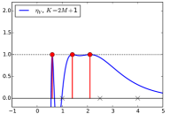
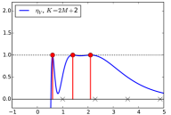
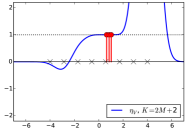
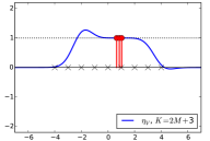
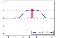
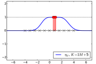
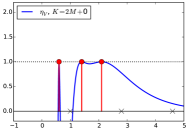
Such is the case of the Laplace filter (see Figure 1), as shown in Section 4, which provides theoretical foundations for the techniques used in [14] for microscopy imaging. Admittedly, the constructed dual certificates decay slowly when going away from the xisubscript𝑥𝑖x_{i}’s, indicating that the stability constants are not so good, and the problem is numerically unstable at large scales. But reconstructing a measure from a few Laplace measurements is a fundamentally difficult problem, and any reconstruction method is bound to face similar limitations. Our results indicate that (8) is able to provide a sound reconstruction method which is robust to small perturbations, at least for a small number of spikes. This property is confirmed by the numerical experiments of [14].

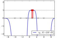
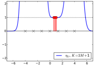
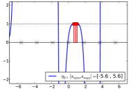
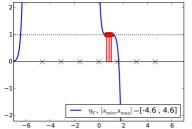
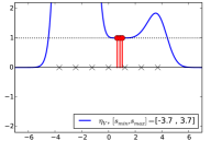
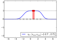
The case of the convolution with a Gaussian kernel is more subtle. We show in Section 4.2 that (7) and (8) yield a support-stable reconstructions provided that the convolution is fully observed (and PSsubscript𝑃𝑆P_{S} is the Lebesgue measure). In general, this property does not hold for any sampling measure PSsubscript𝑃𝑆P_{S}, but it holds for discrete measures PSsubscript𝑃𝑆P_{S} which approximate the Lebesgue measure sufficiently well, see Figure 2. Surprisingly, this support recovery property also holds in the case where the convolution is sampled in a very small interval. We find this “confined sampling” setting quite counter-intuitive, as the samples can be placed anywhere (provided they are in some small interval) with respect to the spikes to recover, contrary e.g. to [2] which requires at least two samples in the neighborhood each spike to recover.
Refer to caption
Refer to caption
Refer to caption
Figure 1: Vanishing derivatives precertificate for Laplace observations (K=2M𝐾2𝑀K=2M, 2M+12𝑀12M+1, and 2M+22𝑀22M+2 measurements). It is sufficient to observe K=2M𝐾2𝑀K=2M samples.
Refer to caption
Refer to caption
Refer to caption
Refer to caption
Refer to caption
Refer to caption
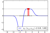
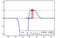
Figure 2: Vanishing derivatives precertificate for the sampled convolution with a Gaussian kernel e(xs)2superscript𝑒superscript𝑥𝑠2e^{-(x-{s})^{2}} (the locations of the samples s𝑠s are indicated by black crosses). The stability criterion (ηV<1subscript𝜂𝑉1\eta_{V}<1) is not always satisfied, but if the sampling measure PSsubscript𝑃𝑆P_{S} approximates the Lebesgue measure sufficiently well, it does hold.
Refer to caption
Refer to caption
Refer to caption
Refer to caption
Refer to caption
Refer to caption
Figure 3: Vanishing derivatives precertificate for the sampled convolution with a Gaussian kernel e(xs)2superscript𝑒superscript𝑥𝑠2e^{-(x-{s})^{2}} (the locations of the samples s𝑠s are indicated by black crosses). If the samples are sufficiently confined (bottom row), the precertificate is valid, ηV<1subscript𝜂𝑉1\eta_{V}<1.

1.1 Previous Works

Discrete 1superscript1\ell^{1} regularization

The use of 1superscript1\ell^{1}-type techniques for the resolution of inverse problems originates from works in geophysics for seismic exploration [9, 39, 31]. Their popularization in signal processing and statistics comes respectively from the seminal works of Donoho [15, 42] and Tibshirani [47]. One usually defines a discrete grid and solves a variational problem on that grid. The literature concerning the robustness of such models is abundant, let us mention [16, 20, 49] which guarantees for exact support recovery, and [21] which bounds the L2superscript𝐿2L^{2} recovery error.

Off-the-grid methods

However, using a discrete grid only approximates the problem to be solved [44, 24], generally breaking the sparsity assumption of the signal (the so-called basis mismatch phenomenon [8]): some resulting artifacts are described in [18]. To circumvent the problem, several researchers [11, 3, 5, 7] proposed to work in a gridless setting, turning the finite dimensional basis pursuit or lasso problems into variational problems in the space of Radon measures. Within that new framework, the notion of minimum separation of the spikes is the cornerstone of several identifiability results [11, 7, 45] as well as robustness results [6, 26, 17]. The particular case of positive sources, which does not impose any separation of the spikes, has been studied in [11, 41] for identifiability, and in [13] for noise robustness (see also [33] in a discrete setup). In dimension d2𝑑2d\geqslant 2, the situation is considerably more difficult, the staility constants are different, as shown in [36].

Non variational methods

Let us also note that, while we focus here on a variant of the Lasso for super-resolution, there is a large panel of methods designed to tackle super-resolution problems. To name a few, MUSIC [35] ESPRIT [27], finite rate-of-innovation [4], matrix pencil [25] or Cadzow denoising [10] techniques are also worth considering. Let us also mention [12, 48] which tackle the super-resolution problem using the (non-convex) tools from sparsity (0superscript0\ell^{0} norm or k𝑘k-sparse vectors). Note that there is a deep connection between super-resolution and machine learning problems such as the recovery of probability densities from random empirical generalized moments [23], which paves the way for efficient methods in the setting of random measurements. It seems that, for a given problem, the method of choice will strongly depend on the desired properties: flexibility on the measurement operator, robustness to noise, ability to handle signals with signs or phases. We do not claim that the Lasso for measures is universally better than the above-mentioned methods, we simply regard (7) as an interesting variational problem that we wish to understand.

1.2 Contributions

In the present work, we propose a necessary and sufficient condition for the Non-Degenerate Source Condition (Theorem 3) which ensures support stability when trying to solve the super-resolution problem using (8). This condition can be seen as some infinitesimal variant of the Determinantal condition in [41], its main advantage is that it ensures the non-vanishing of the second derivatives.

We show that when the observations consist of several samples of an integral transform, it is possible to ensure a priori, for some kernels, that those conditions hold regardless of the positions of the (sufficiently many) samples. Such is the case of the partial Laplace transform or the sampled convolution with a Gaussian (with an L1superscript𝐿1L^{1} normalization). In the case of the unnormalized Gaussian, we show that similar results hold provided the samples approximate the uniform Lebesgue measure sufficiently well, or, on the contrary, if they are drawn in a sufficiently small interval.

The proposed results heavily rely on the techniques introduced in [41] in the field of sparse recovery. Nevertheless, we develop here a self-contained theory, which benefits from the following key differences:

  • Our approach is free of normalization, whereas [41] requires an L1superscript𝐿1L^{1}-type normalization of the atoms. Despite the good empirical results reported in [41], it is arguable whether this normalization is the one to use, as the problem (𝒫λ(y)subscript𝒫𝜆𝑦\mathcal{P}_{\lambda}\left(y\right)) seems naturally Hilbertian. Also, we clarify the relationship between the L1superscript𝐿1L^{1} normalization and the invoked conditions.

  • On a related topic (see Section 3.3), the approach in [41] naturally requires 2M+12𝑀12M+1 observations of the filtered signal (where m0subscript𝑚0m_{0} has M𝑀M spikes), our approach without normalization only needs 2M2𝑀2M, which is the optimal requirement.

  • Most importantly, we ensure the stability of the support at low noise, whereas [41] only provides identifiability.

1.3 Notations and Preliminaries

Functional spaces

Let X𝑋X be an interval of \mathbb{R}. We denote by 𝒞0(X)subscript𝒞0𝑋\mathscr{C}_{0}(X) the space of \mathbb{R}-valued continuous functions which vanish “at infinity”, i.e. for all ε>0𝜀0\varepsilon>0, there exists a compact subset KX𝐾𝑋K\subset X such that

xXK,|η(x)|for-all𝑥𝑋𝐾𝜂𝑥\displaystyle\forall x\in X\setminus K,\quad\left\lvert\eta(x)\right\rvert ε.absent𝜀\displaystyle\leqslant\varepsilon.

More explicitly,

  • If X=[a,b]𝑋𝑎𝑏X=[a,b]\subset\mathbb{R}, 𝒞0(X)=𝒞([a,b])subscript𝒞0𝑋𝒞𝑎𝑏\mathscr{C}_{0}(X)=\mathscr{C}([a,b]) is the space of continuous functions on [a,b]𝑎𝑏[a,b].

  • If X=[a,b)𝑋𝑎𝑏X=[a,b)\subset\mathbb{R}, 𝒞0(X)subscript𝒞0𝑋\mathscr{C}_{0}(X) is the space of continuous functions η𝜂\eta on [a,b)𝑎𝑏[a,b) such that limxbη(x)=0subscript𝑥𝑏𝜂𝑥0\lim_{x\to b}\eta(x)=0.

  • If X=(a,b)𝑋𝑎𝑏X=(a,b)\subseteq\mathbb{R}, 𝒞0(X)subscript𝒞0𝑋\mathscr{C}_{0}(X) is the space of continuous functions η𝜂\eta on (a,b)𝑎𝑏(a,b) such that limxaη(x)=limxbη(x)=0subscript𝑥𝑎𝜂𝑥subscript𝑥𝑏𝜂𝑥0\lim_{x\to a}\eta(x)=\lim_{x\to b}\eta(x)=0.

Endowed with the supremum norm, 𝒞0(X)subscript𝒞0𝑋\mathscr{C}_{0}(X) is a Banach space whose dual is the space b(X)subscript𝑏𝑋\mathcal{M}_{b}(X) of finite Radon measures (see [1]). We denote by b+(X)superscriptsubscript𝑏𝑋\mathcal{M}_{b}^{+}(X) the set of nonnegative Radon measures. In the rest of the paper, we regard 𝒞0(X)subscript𝒞0𝑋\mathscr{C}_{0}(X) and b(X)subscript𝑏𝑋\mathcal{M}_{b}(X) as locally convex topological vector spaces, and we endow them respectively with their weak and weak-* topologies. With that choice, both spaces are dual to each other.

The functional

G(m)𝐺𝑚\displaystyle G(m) =def.m(X)+χb+(X)={m(X)if m is nonnegative,+otherwise.superscriptdef.absent𝑚𝑋subscript𝜒superscriptsubscript𝑏𝑋cases𝑚𝑋if m is nonnegative,otherwise.\displaystyle\stackrel{{\scriptstyle\mbox{\tiny def.}}}{{=}}m(X)+\chi_{\mathcal{M}_{b}^{+}(X)}=\begin{cases}m(X)&\mbox{if $m$ is nonnegative,}\\ +\infty&\mbox{otherwise.}\end{cases}

can be written as a support function

G(m)𝐺𝑚\displaystyle G(m) =sup{Xηdm:η𝒞0(X) and supxXη(x)1},absentsupremumconditional-setsubscript𝑋𝜂differential-d𝑚𝜂subscript𝒞0𝑋 and subscriptsupremum𝑥𝑋𝜂𝑥1\displaystyle=\sup\left\{\int_{X}\eta\mathrm{d}m\;:\;\eta\in\mathscr{C}_{0}(X)\mbox{ and }\sup_{x\in X}{\eta}(x)\leqslant 1\right\},

so that its subdifferential is

G(m)={η𝒞0(X):supη1andXηdm=m(X)}.𝐺𝑚conditional-set𝜂subscript𝒞0𝑋supremum𝜂1andsubscript𝑋𝜂differential-d𝑚𝑚𝑋\displaystyle\partial G(m)=\left\{\eta\in\mathscr{C}_{0}(X)\;:\;\sup{\eta}\leqslant 1\ \mbox{and}\ \int_{X}\eta\mathrm{d}m=m(X)\right\}. (9)
Linear operators

Let \mathcal{H} be a real separable Hilbert space. Let φ𝒞(X;)𝜑𝒞𝑋\varphi\in\mathscr{C}(X;\mathcal{H}) be a continuous \mathcal{H}-valued function such that for all p𝑝p\in\mathcal{H}, (xp,φ(x))𝒞0(X)maps-to𝑥subscript𝑝𝜑𝑥subscript𝒞0𝑋\left(x\mapsto\left\langle p,\,\varphi(x)\right\rangle_{\mathcal{H}}\right)\in\mathscr{C}_{0}(X). Note that by the Banach-Steinhaus theorem, supxXφ(x)<+subscriptsupremum𝑥𝑋subscriptnorm𝜑𝑥\sup_{x\in X}\left\|\varphi(x)\right\|_{\mathcal{H}}<+\infty.

Then, the linear operator Φ:b(X):Φsubscript𝑏𝑋\Phi:\mathcal{M}_{b}(X)\rightarrow\mathcal{H},

Φm=def.Xφdmsuperscriptdef.Φ𝑚subscript𝑋𝜑differential-d𝑚\displaystyle\Phi m\stackrel{{\scriptstyle\mbox{\tiny def.}}}{{=}}\int_{X}\varphi\mathrm{d}m (10)

(where the above quantity is a Bochner integral [50, Sec. V.5]) is weak-* to weak continuous, as shown by the equality

Φm,p=Xφdm,p=Xφ(x),pdm(x).subscriptΦ𝑚𝑝subscriptsubscript𝑋𝜑differential-d𝑚𝑝subscript𝑋subscript𝜑𝑥𝑝differential-d𝑚𝑥\displaystyle\left\langle\Phi m,\,p\right\rangle_{\mathcal{H}}=\left\langle\int_{X}\varphi\mathrm{d}m,\,p\right\rangle_{\mathcal{H}}=\int_{X}\left\langle\varphi(x),\,p\right\rangle_{\mathcal{H}}\mathrm{d}m(x).

It also shows that the adjoint Φ:𝒞0(X):superscriptΦsubscript𝒞0𝑋\Phi^{*}:\mathcal{H}\rightarrow\mathscr{C}_{0}(X) has full domain, with (Φp):xφ(x),p:superscriptΦ𝑝maps-to𝑥subscript𝜑𝑥𝑝(\Phi^{*}p):x\mapsto\left\langle\varphi(x),\,p\right\rangle_{\mathcal{H}}. We note that ΦsuperscriptΦ\Phi^{*} is continuous (from the strong to the strong topology as well as) from the weak to the weak topology.

Admissible Kernels

We say φ𝜑\varphi is in KER(k)superscriptKER𝑘\mbox{{KER}}^{(k)} if φ𝒞k(X;)𝜑superscript𝒞𝑘𝑋\varphi\in\mathscr{C}^{k}(X;\mathcal{H}) and

  • for all p𝑝p\in\mathcal{H}, (xp,φ(x))𝒞0(X)maps-to𝑥subscript𝑝𝜑𝑥subscript𝒞0𝑋\left(x\mapsto\left\langle p,\,\varphi(x)\right\rangle_{\mathcal{H}}\right)\in\mathscr{C}_{0}(X).

  • for all 0ik0𝑖𝑘0\leqslant i\leqslant k, supxXφ(i)(x)<+subscriptsupremum𝑥𝑋subscriptnormsuperscript𝜑𝑖𝑥\sup_{x\in X}\left\|\varphi^{(i)}(x)\right\|_{\mathcal{H}}<+\infty,

Given 𝐱=(x1,,xM)XM𝐱subscript𝑥1subscript𝑥𝑀superscript𝑋𝑀\mathbf{x}=(x_{1},\ldots,x_{M})\in X^{M}, we denote by Φ𝐱:M:subscriptΦ𝐱superscript𝑀\Phi_{\mathbf{x}}:\mathbb{R}^{M}\rightarrow\mathcal{H} the linear operator such that

aM,Φ𝐱(a)=def.i=1Maiφ(xi),formulae-sequencefor-all𝑎superscript𝑀superscriptdef.subscriptΦ𝐱𝑎superscriptsubscript𝑖1𝑀subscript𝑎𝑖𝜑subscript𝑥𝑖\forall a\in\mathbb{R}^{M},\quad\Phi_{\mathbf{x}}(a)\stackrel{{\scriptstyle\mbox{\tiny def.}}}{{=}}\sum_{i=1}^{M}a_{i}\varphi(x_{i}),

and by Γ𝐱:2M:subscriptΓ𝐱superscript2𝑀\Gamma_{\mathbf{x}}:\mathbb{R}^{2M}\rightarrow\mathcal{H} the linear operator defined by

Γ𝐱b=def.i=1M(b2i1φ(xi)+b2iφ(xi)).superscriptdef.subscriptΓ𝐱𝑏superscriptsubscript𝑖1𝑀subscript𝑏2𝑖1𝜑subscript𝑥𝑖subscript𝑏2𝑖superscript𝜑subscript𝑥𝑖\Gamma_{\mathbf{x}}b\stackrel{{\scriptstyle\mbox{\tiny def.}}}{{=}}\sum_{i=1}^{M}\left(b_{2i-1}\varphi(x_{i})+b_{2i}\varphi^{\prime}(x_{i})\right). (11)

We adopt the following matricial notation

Φ𝐱=(φ(x1)φ(xM))andΓ𝐱=(φ(x1),φ(x1)φ(xM),φ(xM)),formulae-sequencesubscriptΦ𝐱𝜑subscript𝑥1𝜑subscript𝑥𝑀andsubscriptΓ𝐱𝜑subscript𝑥1superscript𝜑subscript𝑥1𝜑subscript𝑥𝑀superscript𝜑subscript𝑥𝑀\Phi_{\mathbf{x}}=(\varphi(x_{1})\ \ldots\ \varphi(x_{M}))\quad\text{and}\quad\Gamma_{\mathbf{x}}=(\varphi(x_{1}),\varphi^{\prime}(x_{1})\ \ldots\ \varphi(x_{M}),\varphi^{\prime}(x_{M})),

where the “columns” of those “matrices” are elements of \mathcal{H}. In particular, the adjoint operator Φ𝐱:M:superscriptsubscriptΦ𝐱superscript𝑀\Phi_{\mathbf{x}}^{*}:\mathcal{H}\rightarrow\mathbb{R}^{M} is given by

p,Φ𝐱p=((Φp)(xi))1iM.formulae-sequencefor-all𝑝superscriptsubscriptΦ𝐱𝑝subscriptsuperscriptΦ𝑝subscript𝑥𝑖1𝑖𝑀\forall p\in\mathcal{H},\quad\Phi_{\mathbf{x}}^{*}p=\left((\Phi^{*}p)(x_{i})\right)_{1\leqslant i\leqslant M}.

Given x0Xsubscript𝑥0𝑋x_{0}\in X, we denote by φksubscript𝜑𝑘\varphi_{k}\in\mathcal{H} the kthsuperscript𝑘𝑡k^{th} derivative of φ𝜑\varphi at x0subscript𝑥0x_{0}, i.e.

φk=def.φ(k)(x0).superscriptdef.subscript𝜑𝑘superscript𝜑𝑘subscript𝑥0\varphi_{k}\stackrel{{\scriptstyle\mbox{\tiny def.}}}{{=}}\varphi^{(k)}(x_{0}). (12)

In particular, φ0=φ(x0)subscript𝜑0𝜑subscript𝑥0\varphi_{0}=\varphi(x_{0}).

Given k𝑘k\in\mathbb{N}, we define

Ψk=def.(φ0φ1φk).superscriptdef.subscriptΨ𝑘matrixsubscript𝜑0subscript𝜑1subscript𝜑𝑘\Psi_{k}\stackrel{{\scriptstyle\mbox{\tiny def.}}}{{=}}\begin{pmatrix}\varphi_{0}&\varphi_{1}&\ldots&\varphi_{k}\end{pmatrix}. (13)

If Ψk:k+1:subscriptΨ𝑘superscript𝑘1\Psi_{k}:\mathbb{R}^{k+1}\rightarrow\mathcal{H} has full column rank, we define its pseudo-inverse as Ψk+=def.(ΨkΨk)1Ψksuperscriptdef.superscriptsubscriptΨ𝑘superscriptsuperscriptsubscriptΨ𝑘subscriptΨ𝑘1superscriptsubscriptΨ𝑘\Psi_{k}^{+}\stackrel{{\scriptstyle\mbox{\tiny def.}}}{{=}}(\Psi_{k}^{*}\Psi_{k})^{-1}\Psi_{k}^{*}. Similarly, we denote Γ𝐱+=def.(Γ𝐱Γ𝐱)1Γ𝐱superscriptdef.superscriptsubscriptΓ𝐱superscriptsuperscriptsubscriptΓ𝐱subscriptΓ𝐱1superscriptsubscriptΓ𝐱\Gamma_{\mathbf{x}}^{+}\stackrel{{\scriptstyle\mbox{\tiny def.}}}{{=}}(\Gamma_{\mathbf{x}}^{*}\Gamma_{\mathbf{x}})^{-1}\Gamma_{\mathbf{x}}^{*} provided Γ𝐱subscriptΓ𝐱\Gamma_{\mathbf{x}} has full column rank.

2 The Blasso with nonnegativity constraints

In this section, we describe the main properties of the positive Beurling LASSO (Blasso+) that are needed in the paper. These are mainly minor adaptations of the properties stated in [17, 13] for the Blasso, and we state them here without proof.

We assume that we are given a Hilbert space \mathcal{H} and some kernel φKER(k)𝜑superscriptKER𝑘\varphi\in\mbox{{KER}}^{(k)} for some k2𝑘2k\geqslant 2 as described above. The choice of φ𝜑\varphi and \mathcal{H} is discussed in detail in Section 2.4

2.1 Variational Problems in the Space of Measures

Our goal is to recover an unknown input measure

m0=ma,𝐱=def.i=1Maiδxisubscript𝑚0subscript𝑚𝑎𝐱superscriptdef.superscriptsubscript𝑖1𝑀subscript𝑎𝑖subscript𝛿subscript𝑥𝑖m_{0}=m_{a,\mathbf{x}}\stackrel{{\scriptstyle\mbox{\tiny def.}}}{{=}}\sum_{i=1}^{M}a_{i}\delta_{x_{i}}

with (ai,xi)×Xsubscript𝑎𝑖subscript𝑥𝑖𝑋(a_{i},x_{i})\in\mathbb{R}\times X from the observations y=Φm0+w𝑦Φsubscript𝑚0𝑤y=\Phi m_{0}+w\in\mathcal{H}, where ΦΦ\Phi is the linear operator defined in (10), and w𝑤w\in\mathcal{H} is some additive noise. In this paper, we assume that the amplitudes aisubscript𝑎𝑖a_{i} are positive.

To perform the reconstruction, we solve the following variant of the Blasso, adding a nonnegativity constraint, that we denote by Blasso+,

minmb+(X)λm(X)+12Φmy2,𝑚superscriptsubscript𝑏𝑋𝜆𝑚𝑋12superscriptsubscriptnormΦ𝑚𝑦2\displaystyle\underset{m\in\mathcal{M}_{b}^{+}(X)}{\min}\ \lambda m(X)+\frac{1}{2}\left\|\Phi m-y\right\|_{\mathcal{H}}^{2}, (𝒫λ(y)subscript𝒫𝜆𝑦\mathcal{P}_{\lambda}\left(y\right))

where λ>0𝜆0\lambda>0 is some regularization parameter. In the noiseless case (w=0𝑤0w=0), one might as well solve the constrained problem

minmb+(X)Φm=Φm0m(X).𝑚superscriptsubscript𝑏𝑋Φ𝑚Φsubscript𝑚0𝑚𝑋\displaystyle\underset{\begin{subarray}{c}m\in\mathcal{M}_{b}^{+}(X)\\ \Phi m=\Phi m_{0}\end{subarray}}{\min}\ m(X). (𝒫0(Φm0)subscript𝒫0Φsubscript𝑚0\mathcal{P}_{0}\left(\Phi m_{0}\right))

It worth noting that (𝒫0(Φm0)subscript𝒫0Φsubscript𝑚0\mathcal{P}_{0}\left(\Phi m_{0}\right)) is the limit of (𝒫λ(y)subscript𝒫𝜆𝑦\mathcal{P}_{\lambda}\left(y\right)) as λ0𝜆0\lambda\to 0 and w0subscriptnorm𝑤0\left\|w\right\|_{\mathcal{H}}\to 0 in a suitable way (see [17] for the case of the Blasso).

2.2 Low noise behavior and exact support recovery

From now on, in order to simplify the discussion, we assume that xiint(X)subscript𝑥𝑖int𝑋x_{i}\in\operatorname{int}(X) for all 1iM1𝑖𝑀1\leqslant i\leqslant M, i.e. infX<xi<supXinfimum𝑋subscript𝑥𝑖supremum𝑋\inf X<x_{i}<\sup X.

Exact support recovery

In [17], we have provided an almost sharp sufficient condition for the exact support recovery at low noise. A (simplified) version of that condition is the following. If Γ𝐱subscriptΓ𝐱\Gamma_{\mathbf{x}} (see (11)) has full rank, we define the vanishing derivatives precertificate as

ηVsubscript𝜂𝑉\displaystyle\eta_{V} =def.ΦpV,wheresuperscriptdef.absentsuperscriptΦsubscript𝑝𝑉where\displaystyle\stackrel{{\scriptstyle\mbox{\tiny def.}}}{{=}}\Phi^{*}p_{V},\quad\text{where}\quad (14)
pVsubscript𝑝𝑉\displaystyle p_{V} =def.argmin{p:p,(Φp)(xi)=1,(Φp)(xi)=0for all 1iM}.superscriptdef.absentargmin:subscriptnorm𝑝formulae-sequence𝑝formulae-sequencesuperscriptΦ𝑝subscript𝑥𝑖1superscriptsuperscriptΦ𝑝subscript𝑥𝑖0for all 1iM\displaystyle\stackrel{{\scriptstyle\mbox{\tiny def.}}}{{=}}\operatorname{argmin}\left\{\left\|p\right\|_{\mathcal{H}}\;:\;p\in\mathcal{H},(\Phi^{*}p)(x_{i})=1,(\Phi^{*}p)^{\prime}(x_{i})=0\ \mbox{for all $1\leqslant i\leqslant M$}\right\}. (15)

In other words, pV=Γx+,usubscript𝑝𝑉superscriptsubscriptΓ𝑥𝑢p_{V}=\Gamma_{x}^{+,*}u where u=def.(1,0,1,0,1,0)T2Msuperscriptdef.𝑢superscript101010𝑇superscript2𝑀u\stackrel{{\scriptstyle\mbox{\tiny def.}}}{{=}}(1,0,1,0\ldots,1,0)^{T}\in\mathbb{R}^{2M}, and Γx+,=Γx(ΓxΓx)1superscriptsubscriptΓ𝑥subscriptΓ𝑥superscriptsuperscriptsubscriptΓ𝑥subscriptΓ𝑥1\Gamma_{x}^{+,*}=\Gamma_{x}(\Gamma_{x}^{*}\Gamma_{x})^{-1} is the Moore-Penrose pseudo-inverse of ΓxsubscriptΓ𝑥\Gamma_{x}. We note that by optimality of pVsubscript𝑝𝑉p_{V} in (14), there exists some coefficients {αi,βi}1iMsubscriptsubscript𝛼𝑖subscript𝛽𝑖1𝑖𝑀\{\alpha_{i},\beta_{i}\}_{1\leqslant i\leqslant M}\subset\mathbb{R} such that pV=i=1M(αiφ(xi)+βiφ(xi))subscript𝑝𝑉superscriptsubscript𝑖1𝑀subscript𝛼𝑖𝜑subscript𝑥𝑖subscript𝛽𝑖superscript𝜑subscript𝑥𝑖p_{V}=\sum_{i=1}^{M}\left(\alpha_{i}\varphi(x_{i})+\beta_{i}\varphi^{\prime}(x_{i})\right), and ηVsubscript𝜂𝑉\eta_{V} is the unique function of the form

ηV(x)subscript𝜂𝑉𝑥\displaystyle\eta_{V}(x) =i=1M(αiφ(x),φ(xi)+βiφ(x),φ(xi))absentsuperscriptsubscript𝑖1𝑀subscript𝛼𝑖subscript𝜑𝑥𝜑subscript𝑥𝑖subscript𝛽𝑖subscriptsuperscript𝜑𝑥superscript𝜑subscript𝑥𝑖\displaystyle=\sum_{i=1}^{M}\left(\alpha_{i}\left\langle\varphi(x),\,\varphi(x_{i})\right\rangle_{\mathcal{H}}+\beta_{i}\left\langle\varphi^{\prime}(x),\,\varphi^{\prime}(x_{i})\right\rangle_{\mathcal{H}}\right) (16)

which satisfies ηV(xi)=1subscript𝜂𝑉subscript𝑥𝑖1\eta_{V}(x_{i})=1 and ηV(xi)=0superscriptsubscript𝜂𝑉subscript𝑥𝑖0\eta_{V}^{\prime}(x_{i})=0 for all i{1,,M}𝑖1𝑀i\in\{1,\ldots,M\}.

Definition 1 (NDSC).

Assume that Γ𝐱subscriptΓ𝐱\Gamma_{\mathbf{x}} has full rank. We say that m0subscript𝑚0m_{0} satisfies the Non Degenerate Source Condition if ηV(x)<1subscript𝜂𝑉𝑥1\eta_{V}(x)<1 for all xX{x1,,xM}𝑥𝑋subscript𝑥1subscript𝑥𝑀x\in X\setminus\{x_{1},\ldots,x_{M}\} and ηV′′(xi)<0superscriptsubscript𝜂𝑉′′subscript𝑥𝑖0\eta_{V}^{\prime\prime}(x_{i})<0 for all 1iM1𝑖𝑀1\leqslant i\leqslant M.

As the next result shows, the nondegeneracy of ηVsubscript𝜂𝑉\eta_{V} almost characterizes the support stability of the Blasso+at low noise. When it holds, it entails |a~i(λ,w)ai|=O(w)subscript~𝑎𝑖𝜆𝑤subscript𝑎𝑖𝑂subscriptnorm𝑤\left\lvert\tilde{a}_{i}(\lambda,w)-a_{i}\right\rvert=O(\left\|w\right\|_{\mathcal{H}}) and |x~i(λ,w)xi|=O(w)subscript~𝑥𝑖𝜆𝑤subscript𝑥𝑖𝑂subscriptnorm𝑤\left\lvert\tilde{x}_{i}(\lambda,w)-x_{i}\right\rvert=O(\left\|w\right\|_{\mathcal{H}}) for λ=1αw𝜆1𝛼subscriptnorm𝑤\lambda=\frac{1}{\alpha}\left\|w\right\|_{\mathcal{H}}.

Theorem 1 ([17]).

Assume that Γ𝐱subscriptΓ𝐱\Gamma_{\mathbf{x}} has full rank and that m0subscript𝑚0m_{0} satisfies the Non Degenerate Source Condition. Then there exists α>0𝛼0\alpha>0, λ0>0subscript𝜆00\lambda_{0}>0 such that for all 0λλ00𝜆subscript𝜆00\leqslant\lambda\leqslant\lambda_{0} and wαλsubscriptnorm𝑤𝛼𝜆\left\|w\right\|_{\mathcal{H}}\leqslant\alpha\lambda, the solution m~λ,wsubscript~𝑚𝜆𝑤\tilde{m}_{\lambda,w} to (𝒫λ(y)subscript𝒫𝜆𝑦\mathcal{P}_{\lambda}\left(y\right)) is unique and is composed of exactly M𝑀M spikes, with m~0,0=m0subscript~𝑚00subscript𝑚0\tilde{m}_{0,0}=m_{0}.

Moreover one may write m~λ,w=i=0Ma~i(λ,w)δx~i(λ,w)subscript~𝑚𝜆𝑤superscriptsubscript𝑖0𝑀subscript~𝑎𝑖𝜆𝑤subscript𝛿subscript~𝑥𝑖𝜆𝑤\tilde{m}_{\lambda,w}=\sum_{i=0}^{M}\tilde{a}_{i}(\lambda,w)\delta_{\tilde{x}_{i}(\lambda,w)}, where a~isubscript~𝑎𝑖\tilde{a}_{i} and x~isubscript~𝑥𝑖\tilde{x}_{i} are the restriction of 𝒞1superscript𝒞1\mathscr{C}^{1} functions on a neighborhood of (0,0)00(0,0).

Conversely, if Γ𝐱subscriptΓ𝐱\Gamma_{\mathbf{x}} has full rank and the solutions can be written in the above form with functions a~isubscript~𝑎𝑖\tilde{a}_{i} and x~isubscript~𝑥𝑖\tilde{x}_{i} which are 𝒞1superscript𝒞1\mathscr{C}^{1} and satisfy a~i(0,0)=aisubscript~𝑎𝑖00subscript𝑎𝑖\tilde{a}_{i}(0,0)=a_{i}, x~i(0,0)=xisubscript~𝑥𝑖00subscript𝑥𝑖\tilde{x}_{i}(0,0)=x_{i}, then ηV1subscript𝜂𝑉1\eta_{V}\leqslant 1.

Unfortunately, the Non Degenerate Source Condition (NDSC) is not trivial to ensure a priori. One reason is that it should be checked for any configuration x1<<xMsubscript𝑥1subscript𝑥𝑀x_{1}<\ldots<x_{M}. Let us mention [46] which proves that the (NDSC) holds for the Gaussian or Cauchy kernels and signed measures, provided the spikes are sufficiently separated. As noted above in the introduction, in the signed case, the (NDSC) generally cannot hold if spikes with opposite signs are too close (see [17, Corollary 1] and [43]).

The situation is more favorable in the setting of nonnegative measures that we consider. In Section 3, building upon [41], we show that the (NDSC) holds for specific choices of φ𝜑\varphi which include the Laplace kernel.

The case of clustered spikes

Another approach for nonnegative measures, taken in [13], is to consider spikes which are located in a small neighborhood of a single point x0int(X)subscript𝑥0int𝑋x_{0}\in\operatorname{int}(X), say xi=x0+tzisubscript𝑥𝑖subscript𝑥0𝑡subscript𝑧𝑖x_{i}=x_{0}+tz_{i}, for some zisubscript𝑧𝑖z_{i}\in\mathbb{R} and some small t>0𝑡0t>0. Let us write mt=i=1Maiδx0+tzisubscript𝑚𝑡superscriptsubscript𝑖1𝑀subscript𝑎𝑖subscript𝛿subscript𝑥0𝑡subscript𝑧𝑖m_{t}=\sum_{i=1}^{M}a_{i}\delta_{x_{0}+tz_{i}} and yt=Φmt+wsubscript𝑦𝑡Φsubscript𝑚𝑡𝑤y_{t}=\Phi m_{t}+w. One may prove that, as t0+𝑡superscript0t\to 0^{+}, the corresponding pVsubscript𝑝𝑉p_{V} converges (strongly in \mathcal{H}) towards

pW=argmin{pW:(ΦpW)(x0)=1,(ΦpW)(x0)==(ΦpW)(2M1)(x0)=0}subscript𝑝𝑊argmin:subscriptnormsubscript𝑝𝑊formulae-sequencesuperscriptΦsubscript𝑝𝑊subscript𝑥01superscriptsuperscriptΦsubscript𝑝𝑊subscript𝑥0superscriptsuperscriptΦsubscript𝑝𝑊2𝑀1subscript𝑥00\displaystyle p_{W}=\operatorname{argmin}\left\{\left\|p_{W}\right\|_{\mathcal{H}}\;:\;(\Phi^{*}p_{W})(x_{0})=1,(\Phi^{*}p_{W})^{\prime}(x_{0})=\ldots=(\Phi^{*}p_{W})^{(2M-1)}(x_{0})=0\right\} (17)

provided φKER(2M1)𝜑superscriptKER2𝑀1\varphi\in\mbox{{KER}}^{(2M-1)} and (φ0,,φ2M1)subscript𝜑0subscript𝜑2𝑀1(\varphi_{0},\ldots,\varphi_{2M-1}) has full rank. As a result ηV=ΦpVsubscript𝜂𝑉superscriptΦsubscript𝑝𝑉\eta_{V}=\Phi^{*}p_{V} converges (uniformly on X𝑋X) towards ηW=def.ΦpWsuperscriptdef.subscript𝜂𝑊superscriptΦsubscript𝑝𝑊\eta_{W}\stackrel{{\scriptstyle\mbox{\tiny def.}}}{{=}}\Phi^{*}p_{W}, and the same holds for the derivatives up to the regularity of φ𝜑\varphi. Letting Ψ2M1=def.(φ0,,φ2M1)superscriptdef.subscriptΨ2𝑀1subscript𝜑0subscript𝜑2𝑀1\Psi_{2M-1}\stackrel{{\scriptstyle\mbox{\tiny def.}}}{{=}}(\varphi_{0},\ldots,\varphi_{2M-1}), we note as above that pW=def.Ψ2M1+,vsuperscriptdef.subscript𝑝𝑊superscriptsubscriptΨ2𝑀1𝑣p_{W}\stackrel{{\scriptstyle\mbox{\tiny def.}}}{{=}}\Psi_{2M-1}^{+,*}v where v=def.(1,0,,0)T2Msuperscriptdef.𝑣superscript100𝑇superscript2𝑀v\stackrel{{\scriptstyle\mbox{\tiny def.}}}{{=}}(1,0,\ldots,0)^{T}\in\mathbb{R}^{2M}. Moreover, ηWsubscript𝜂𝑊\eta_{W} is the unique the function of the form

ηW:xk=02M1βkφ(x),φ(k)(x0),:subscript𝜂𝑊maps-to𝑥superscriptsubscript𝑘02𝑀1subscript𝛽𝑘subscript𝜑𝑥superscript𝜑𝑘subscript𝑥0\eta_{W}:x\mapsto\sum_{k=0}^{2M-1}\beta_{k}\left\langle\varphi(x),\,\varphi^{(k)}(x_{0})\right\rangle_{\mathcal{H}},

which satisfies

ηW(x0)=1,ηW(x0)=0,,ηW(2M1)(x0)=0.formulae-sequencesubscript𝜂𝑊subscript𝑥01formulae-sequencesuperscriptsubscript𝜂𝑊subscript𝑥00superscriptsubscript𝜂𝑊2𝑀1subscript𝑥00\eta_{W}(x_{0})=1,\ \eta_{W}^{\prime}(x_{0})=0,\ \ldots,\ \eta_{W}^{(2M-1)}(x_{0})=0. (18)
Definition 2 ((2M1)2𝑀1(2M-1)-Nondegeneracy).

We say that a point x0subscript𝑥0x_{0} is (2M1)2𝑀1(2M-1) Non Degenerate if

  • φKER(2M)𝜑superscriptKER2𝑀\varphi\in\mbox{{KER}}^{(2M)},

  • Ψ2M1=def.(φ0,,φ2M1)superscriptdef.subscriptΨ2𝑀1subscript𝜑0subscript𝜑2𝑀1\Psi_{2M-1}\stackrel{{\scriptstyle\mbox{\tiny def.}}}{{=}}(\varphi_{0},\ldots,\varphi_{2M-1}) has full rank,

  • ηW(2M)(x0)<0superscriptsubscript𝜂𝑊2𝑀subscript𝑥00\eta_{W}^{(2M)}(x_{0})<0,

  • for all xX{x0}𝑥𝑋subscript𝑥0x\in X\setminus\{x_{0}\}, ηW(x0)<1subscript𝜂𝑊subscript𝑥01\eta_{W}(x_{0})<1.

The (2M1)2𝑀1(2M-1)-Nondegeneracy of a point entails the support stability of finite measures which are clustered around x0subscript𝑥0x_{0}.

Theorem 2 ([13]).

Assume that φKER(2M+1)𝜑superscriptKER2𝑀1\varphi\in\mbox{{KER}}^{(2M+1)} and that the point is (2M1)2𝑀1(2M-1) Non Degenerate. Then there exists t0>0subscript𝑡00t_{0}>0, such that mtsubscript𝑚𝑡m_{t} satisfies the (NDSC) for for all 0<t<t00𝑡subscript𝑡00<t<t_{0}.

More precisely, there exists α>0𝛼0\alpha>0, CR>0subscript𝐶𝑅0C_{R}>0 and C>0𝐶0C>0 such that for 0<t<t00𝑡subscript𝑡00<t<t_{0} and all 0<λ+w<CRt2M1evaluated-at0bralimit-from𝜆𝑤subscript𝐶𝑅superscript𝑡2𝑀10<\lambda+\left\|w\right\|_{\mathcal{H}}<C_{R}t^{2M-1} with wαλsubscriptnorm𝑤𝛼𝜆\left\|w\right\|_{\mathcal{H}}\leqslant\alpha\lambda,

  • the problem 𝒫λ(yt)subscript𝒫𝜆subscript𝑦𝑡\mathcal{P}_{\lambda}\left(y_{t}\right) has a unique solution of the form i=1Mai~(λ,w,t)δx0+tz~i(λ,w,t)superscriptsubscript𝑖1𝑀~subscript𝑎𝑖𝜆𝑤𝑡subscript𝛿subscript𝑥0𝑡subscript~𝑧𝑖𝜆𝑤𝑡\sum_{i=1}^{M}\tilde{a_{i}}(\lambda,w,t)\delta_{x_{0}+t\tilde{z}_{i}(\lambda,w,t)},

  • the mapping gt:(λ,w)(ai~,z~i):subscript𝑔𝑡maps-to𝜆𝑤~subscript𝑎𝑖subscript~𝑧𝑖g_{t}:(\lambda,w)\mapsto(\tilde{a_{i}},\tilde{z}_{i}) is the restriction of a 𝒞2Msuperscript𝒞2𝑀\mathscr{C}^{2M} function,

  • the following inequality holds

    |(a~,z~)(a,z)|C(|λ|t2M1+wt2M1).subscript~𝑎~𝑧𝑎𝑧𝐶𝜆superscript𝑡2𝑀1subscriptnorm𝑤superscript𝑡2𝑀1\displaystyle\left\lvert(\tilde{a},\tilde{z})-(a,z)\right\rvert_{\infty}\leqslant C\left(\frac{\left\lvert\lambda\right\rvert}{t^{2M-1}}+\frac{\left\|w\right\|_{\mathcal{H}}}{t^{2M-1}}\right).

Theorem 2 is more quantitative than Theorem 1, as it gives the scaling of the constants with respect to the spacing t𝑡t of the spikes, describing how it becomes ill-conditioned.

2.3 Ensuring negative second derivatives

In general, the conditions ηV′′(xi)<0superscriptsubscript𝜂𝑉′′subscript𝑥𝑖0\eta_{V}^{\prime\prime}(x_{i})<0 and ηW(2M)(x0)<0superscriptsubscript𝜂𝑊2𝑀subscript𝑥00\eta_{W}^{(2M)}(x_{0})<0 in the non degeneracy hypotheses are difficult to ensure a priori. They can be checked numerically, or, in the case of ηWsubscript𝜂𝑊\eta_{W}, analytically on a closed form expression. But it is sometimes possible to ensure them a priori: in [13, Proposition 5], we have proved that ηW(2M)(x0)<0superscriptsubscript𝜂𝑊2𝑀subscript𝑥00\eta_{W}^{(2M)}(x_{0})<0 for fully sampled convolutions on translation-invariant domains, under a mild assumption.

In the present paper we propose the following two new Lemmas, which work for any sampling of the impulse response. They follow directly from (16) and the characterization of ηVsubscript𝜂𝑉\eta_{V}, in the spirit of Cramer’s rule.

Lemma 1.

Assume that Γ𝐱subscriptΓ𝐱\Gamma_{\mathbf{x}} has full rank. Then for all i{1,,M}𝑖1𝑀i\in\{1,\ldots,M\},

|φ(x1),φ(x1)φ(x1),φ(x1)φ(x1),φ(xM)1φ(x1),φ(x1)φ(x1),φ(x1)φ(x1),φ(xM)0φ(xM),φ(x1)φ(xM),φ(x1)φ(xM),φ(xM)1φ(xM),φ(x1)φ(xM),φ(x1)φ(xM),φ(xM)0φ′′(xi),φ(x1)φ′′(xi),φ(x1)φ′′(xi),φ(xM)0|=ηV′′(xi)det(Γ𝐱Γ𝐱).matrixsubscript𝜑subscript𝑥1𝜑subscript𝑥1subscript𝜑subscript𝑥1superscript𝜑subscript𝑥1subscript𝜑subscript𝑥1superscript𝜑subscript𝑥𝑀1subscriptsuperscript𝜑subscript𝑥1𝜑subscript𝑥1subscriptsuperscript𝜑subscript𝑥1superscript𝜑subscript𝑥1subscriptsuperscript𝜑subscript𝑥1superscript𝜑subscript𝑥𝑀0missing-subexpressionsubscript𝜑subscript𝑥𝑀𝜑subscript𝑥1subscript𝜑subscript𝑥𝑀superscript𝜑subscript𝑥1subscript𝜑subscript𝑥𝑀superscript𝜑subscript𝑥𝑀1subscriptsuperscript𝜑subscript𝑥𝑀𝜑subscript𝑥1subscriptsuperscript𝜑subscript𝑥𝑀superscript𝜑subscript𝑥1subscriptsuperscript𝜑subscript𝑥𝑀superscript𝜑subscript𝑥𝑀0subscriptsuperscript𝜑′′subscript𝑥𝑖𝜑subscript𝑥1subscriptsuperscript𝜑′′subscript𝑥𝑖superscript𝜑subscript𝑥1subscriptsuperscript𝜑′′subscript𝑥𝑖superscript𝜑subscript𝑥𝑀0superscriptsubscript𝜂𝑉′′subscript𝑥𝑖superscriptsubscriptΓ𝐱subscriptΓ𝐱\displaystyle\begin{vmatrix}\left\langle\varphi(x_{1}),\,\varphi(x_{1})\right\rangle_{\mathcal{H}}&\left\langle\varphi(x_{1}),\,\varphi^{\prime}(x_{1})\right\rangle_{\mathcal{H}}&\cdots&\left\langle\varphi(x_{1}),\,\varphi^{\prime}(x_{M})\right\rangle_{\mathcal{H}}&1\\ \left\langle\varphi^{\prime}(x_{1}),\,\varphi(x_{1})\right\rangle_{\mathcal{H}}&\left\langle\varphi^{\prime}(x_{1}),\,\varphi^{\prime}(x_{1})\right\rangle_{\mathcal{H}}&\cdots&\left\langle\varphi^{\prime}(x_{1}),\,\varphi^{\prime}(x_{M})\right\rangle_{\mathcal{H}}&0\\ \vdots&\vdots&&\vdots&\vdots\\ \left\langle\varphi(x_{M}),\,\varphi(x_{1})\right\rangle_{\mathcal{H}}&\left\langle\varphi(x_{M}),\,\varphi^{\prime}(x_{1})\right\rangle_{\mathcal{H}}&\cdots&\left\langle\varphi(x_{M}),\,\varphi^{\prime}(x_{M})\right\rangle_{\mathcal{H}}&1\\ \left\langle\varphi^{\prime}(x_{M}),\,\varphi(x_{1})\right\rangle_{\mathcal{H}}&\left\langle\varphi^{\prime}(x_{M}),\,\varphi^{\prime}(x_{1})\right\rangle_{\mathcal{H}}&\cdots&\left\langle\varphi^{\prime}(x_{M}),\,\varphi^{\prime}(x_{M})\right\rangle_{\mathcal{H}}&0\\ \left\langle\varphi^{\prime\prime}(x_{i}),\,\varphi(x_{1})\right\rangle_{\mathcal{H}}&\left\langle\varphi^{\prime\prime}(x_{i}),\,\varphi^{\prime}(x_{1})\right\rangle_{\mathcal{H}}&\cdots&\left\langle\varphi^{\prime\prime}(x_{i}),\,\varphi^{\prime}(x_{M})\right\rangle_{\mathcal{H}}&0\end{vmatrix}=-\eta_{V}^{\prime\prime}(x_{i})\det(\Gamma_{\mathbf{x}}^{*}\Gamma_{\mathbf{x}}). (19)

Ensuring that the left hand side is positive provides the condition ηV′′(xM)<0superscriptsubscript𝜂𝑉′′subscript𝑥𝑀0\eta_{V}^{\prime\prime}(x_{M})<0, and a similar argument can be derived for the other xisubscript𝑥𝑖x_{i}’s.

The analogous property for ηWsubscript𝜂𝑊\eta_{W} is the following.

Lemma 2.

Assume that Ψ2M1subscriptΨ2𝑀1\Psi_{2M-1} has full column rank.

Then,

|φ0,φ0φ0,φ1φ0,φ2M11φ1,φ0φ1,φ1φ1,φ2M10φ2M,φ0φ2M,φ1φ2M,φ2M10|matrixsubscriptsubscript𝜑0subscript𝜑0subscriptsubscript𝜑0subscript𝜑1subscriptsubscript𝜑0subscript𝜑2𝑀11subscriptsubscript𝜑1subscript𝜑0subscriptsubscript𝜑1subscript𝜑1subscriptsubscript𝜑1subscript𝜑2𝑀10missing-subexpressionsubscriptsubscript𝜑2𝑀subscript𝜑0subscriptsubscript𝜑2𝑀subscript𝜑1subscriptsubscript𝜑2𝑀subscript𝜑2𝑀10\displaystyle\begin{vmatrix}\left\langle\varphi_{0},\,\varphi_{0}\right\rangle_{\mathcal{H}}&\left\langle\varphi_{0},\,\varphi_{1}\right\rangle_{\mathcal{H}}&\cdots&\left\langle\varphi_{0},\,\varphi_{2M-1}\right\rangle_{\mathcal{H}}&1\\ \left\langle\varphi_{1},\,\varphi_{0}\right\rangle_{\mathcal{H}}&\left\langle\varphi_{1},\,\varphi_{1}\right\rangle_{\mathcal{H}}&\cdots&\left\langle\varphi_{1},\,\varphi_{2M-1}\right\rangle_{\mathcal{H}}&0\\ \vdots&\vdots&&\vdots&\vdots\\ \left\langle\varphi_{2M},\,\varphi_{0}\right\rangle_{\mathcal{H}}&\left\langle\varphi_{2M},\,\varphi_{1}\right\rangle_{\mathcal{H}}&\cdots&\left\langle\varphi_{2M},\,\varphi_{2M-1}\right\rangle_{\mathcal{H}}&0\end{vmatrix} =ηW(2M)(x0)det(Ψ2M1Ψ2M1).absentsuperscriptsubscript𝜂𝑊2𝑀subscript𝑥0superscriptsubscriptΨ2𝑀1subscriptΨ2𝑀1\displaystyle=-\eta_{W}^{(2M)}(x_{0})\det(\Psi_{2M-1}^{*}\Psi_{2M-1}). (20)

2.4 Reconstruction frameworks

Now, we discuss the choice of the Hilbert space and kernel φ𝜑\varphi .

Remark 1.

Let us note that (𝒫λ(y)subscript𝒫𝜆𝑦\mathcal{P}_{\lambda}\left(y\right)) may be written in terms of the autocorrelation function

(x,x)X2,Rφ(x,x)=def.φ(x),φ(x).formulae-sequencefor-all𝑥superscript𝑥superscript𝑋2superscriptdef.subscript𝑅𝜑𝑥superscript𝑥subscript𝜑𝑥𝜑superscript𝑥\forall\,(x,x^{\prime})\in X^{2},\quad R_{\varphi}(x,x^{\prime})\stackrel{{\scriptstyle\mbox{\tiny def.}}}{{=}}\left\langle\varphi(x),\,\varphi(x^{\prime})\right\rangle_{\mathcal{H}}.

Introducing the autocorrelation operator

𝐑φ=def.ΦΦ:b(X):superscriptdef.subscript𝐑𝜑superscriptΦΦsubscript𝑏𝑋\displaystyle\mathbf{R}_{\varphi}\stackrel{{\scriptstyle\mbox{\tiny def.}}}{{=}}\Phi^{*}\Phi\colon\mathcal{M}_{b}(X) 𝒞0(X)absentsubscript𝒞0𝑋\displaystyle\rightarrow\mathscr{C}_{0}(X)
m𝑚\displaystyle m (XRφ(,x)dm(x)),absentsubscript𝑋subscript𝑅𝜑superscript𝑥differential-d𝑚superscript𝑥\displaystyle\longmapsto\left(\int_{X}R_{\varphi}(\cdot,x^{\prime})\mathrm{d}m(x^{\prime})\right),

we note that (𝒫λ(y)subscript𝒫𝜆𝑦\mathcal{P}_{\lambda}\left(y\right)) is equivalent to

12y2+minmb+(X)(λm(X)+12𝐑φm,mΦy,m)12superscriptsubscriptnorm𝑦2𝑚superscriptsubscript𝑏𝑋𝜆𝑚𝑋12subscript𝐑𝜑𝑚𝑚superscriptΦ𝑦𝑚\frac{1}{2}\left\|y\right\|_{\mathcal{H}}^{2}+\underset{m\in\mathcal{M}_{b}^{+}(X)}{\min}\;\left(\lambda m(X)+\frac{1}{2}\left\langle\mathbf{R}_{\varphi}m,\,m\right\rangle-\left\langle\Phi^{*}y,\,m\right\rangle\right) (𝒫~y~𝒫𝑦\tilde{\mathcal{P}}{y})

(here ,\left\langle\cdot,\,\cdot\right\rangle denotes the duality pairing between 𝒞0(X)subscript𝒞0𝑋\mathscr{C}_{0}(X) and b(X)subscript𝑏𝑋\mathcal{M}_{b}(X)). As a result, everything described above (in particular expression for certificates) can be written in term of the autocorrelation function and its derivatives. Moreover, choosing φ𝜑\varphi and \mathcal{H} is equivalent (but less intuitive) to choosing the autocorrelation function Rφsubscript𝑅𝜑R_{\varphi}.

A typical choice of Hilbert space covered by our framework is the following. Given some positive measure PSsubscript𝑃𝑆P_{S} on some interval S𝑆S\subseteq\mathbb{R}, the impulse response is

φ(x):sψ(x,s):𝜑𝑥maps-to𝑠𝜓𝑥𝑠\displaystyle\varphi(x):{s}\mapsto\psi(x,{s})

where ψ𝜓\psi is some kernel and =L2(S,PS)superscriptL2𝑆subscript𝑃𝑆\mathcal{H}=\text{L}^{2}(S,P_{S}). We say that (S,PS)𝑆subscript𝑃𝑆(S,P_{S}) define a reconstruction framework.

For instance, if PS=k=1Kδsksubscript𝑃𝑆superscriptsubscript𝑘1𝐾subscript𝛿subscript𝑠𝑘P_{S}=\sum_{k=1}^{K}\delta_{{s}_{k}} and ψ(x,s)=e(xs)2𝜓𝑥𝑠superscript𝑒superscript𝑥𝑠2\psi(x,{s})=e^{-(x-{s})^{2}}, our observation is the sampled convolution of m0subscript𝑚0m_{0} with the Gaussian kernel,

(Φm0)k=Xe(xsk)dm0(x),subscriptΦsubscript𝑚0𝑘subscript𝑋superscript𝑒𝑥subscript𝑠𝑘differential-dsubscript𝑚0𝑥\displaystyle(\Phi m_{0})_{k}=\int_{X}e^{-(x-{s}_{k})}\mathrm{d}m_{0}(x),

and the norm of \mathcal{H} is the standard Euclidean norm in Ksuperscript𝐾\mathbb{R}^{K}.

In the following, we usually assume that ψ𝜓\psi is smooth in its first argument, and that it is possible to differentiate under the sum symbol,

φ(k)(x)=(1)kψ(x,)L2(S,PS).superscript𝜑𝑘𝑥superscriptsubscript1𝑘𝜓𝑥superscriptL2𝑆subscript𝑃𝑆\displaystyle\varphi^{(k)}(x)=(\partial_{1})^{k}\psi(x,\cdot)\in\text{L}^{2}(S,P_{S}). (21)

3 A characterization of the Non-Degenerate Source Condition

In this section we provide a simple criterion which ensures that a measure m0subscript𝑚0m_{0} is the unique solution to the basis pursuit for measures (𝒫0(Φm0)subscript𝒫0Φsubscript𝑚0\mathcal{P}_{0}\left(\Phi m_{0}\right)), and that its recovery using (𝒫λ(y)subscript𝒫𝜆𝑦\mathcal{P}_{\lambda}\left(y\right)) is stable. This criterion is an ”infinitesimal version” of the criterion proposed in [41], except that we do not impose any normalisation of the atoms (nor any weight on the total variation). Throughout this section we let {xi}i=1Mint(X)superscriptsubscriptsubscript𝑥𝑖𝑖1𝑀int𝑋\{x_{i}\}_{i=1}^{M}\subset\operatorname{int}(X) with x1<<xMsubscript𝑥1subscript𝑥𝑀x_{1}<\ldots<x_{M}, and x0int(X)subscript𝑥0int𝑋x_{0}\in\operatorname{int}(X).

3.1 Rescaled determinants

The following elementary result is a specialization of a standard trick in the study of extended T-systems [29]. For sufficiently regular functions {u0,,u2M}subscript𝑢0subscript𝑢2𝑀\{u_{0},\ldots,u_{2M}\}, define DVsubscript𝐷𝑉D_{V} and DWsubscript𝐷𝑊D_{W} by

tX{xi}i=1M,DV(t)for-all𝑡𝑋superscriptsubscriptsubscript𝑥𝑖𝑖1𝑀subscript𝐷𝑉𝑡\displaystyle\forall t\in X\setminus\{x_{i}\}_{i=1}^{M},\quad D_{V}(t) =def.2i=1M(txi)2|u0(t)u1(t)u2M(t)u0(x1)u1(x1)u2M(x1)u0(x1)u1(x1)u2M(x1)u0(xM)u1(xM)u2M(xM)u0(xM)u1(xM)u2M(xM)|,superscriptdef.absent2superscriptsubscriptproduct𝑖1𝑀superscript𝑡subscript𝑥𝑖2matrixsubscript𝑢0𝑡subscript𝑢1𝑡subscript𝑢2𝑀𝑡subscript𝑢0subscript𝑥1subscript𝑢1subscript𝑥1subscript𝑢2𝑀subscript𝑥1superscriptsubscript𝑢0subscript𝑥1superscriptsubscript𝑢1subscript𝑥1superscriptsubscript𝑢2𝑀subscript𝑥1missing-subexpressionsubscript𝑢0subscript𝑥𝑀subscript𝑢1subscript𝑥𝑀subscript𝑢2𝑀subscript𝑥𝑀superscriptsubscript𝑢0subscript𝑥𝑀superscriptsubscript𝑢1subscript𝑥𝑀superscriptsubscript𝑢2𝑀subscript𝑥𝑀\displaystyle\stackrel{{\scriptstyle\mbox{\tiny def.}}}{{=}}\frac{2}{\prod_{i=1}^{M}(t-x_{i})^{2}}\begin{vmatrix}u_{0}(t)&u_{1}(t)&\cdots&u_{2M}(t)\\ u_{0}(x_{1})&u_{1}(x_{1})&\cdots&u_{2M}(x_{1})\\ u_{0}^{\prime}(x_{1})&u_{1}^{\prime}(x_{1})&\cdots&u_{2M}^{\prime}(x_{1})\\ \vdots&\vdots&&\vdots\\ u_{0}(x_{M})&u_{1}(x_{M})&\cdots&u_{2M}(x_{M})\\ u_{0}^{\prime}(x_{M})&u_{1}^{\prime}(x_{M})&\cdots&u_{2M}^{\prime}(x_{M})\end{vmatrix}, (22)
tX{x0},DW(t)for-all𝑡𝑋subscript𝑥0subscript𝐷𝑊𝑡\displaystyle\forall t\in X\setminus\{x_{0}\},\quad D_{W}(t) =def.(2M)!(tx0)2M|u0(t)u1(t)u2M(t)u0(x1)u1(x1)u2M(x1)u0(x1)u1(x1)u2M(x1)u0(2M1)(xM)u1(2M1)(xM)u2M(2M1)(xM)|.superscriptdef.absent2𝑀superscript𝑡subscript𝑥02𝑀matrixsubscript𝑢0𝑡subscript𝑢1𝑡subscript𝑢2𝑀𝑡subscript𝑢0subscript𝑥1subscript𝑢1subscript𝑥1subscript𝑢2𝑀subscript𝑥1superscriptsubscript𝑢0subscript𝑥1superscriptsubscript𝑢1subscript𝑥1superscriptsubscript𝑢2𝑀subscript𝑥1missing-subexpressionsuperscriptsubscript𝑢02𝑀1subscript𝑥𝑀superscriptsubscript𝑢12𝑀1subscript𝑥𝑀superscriptsubscript𝑢2𝑀2𝑀1subscript𝑥𝑀\displaystyle\stackrel{{\scriptstyle\mbox{\tiny def.}}}{{=}}\frac{(2M)!}{(t-x_{0})^{2M}}\begin{vmatrix}u_{0}(t)&u_{1}(t)&\cdots&u_{2M}(t)\\ u_{0}(x_{1})&u_{1}(x_{1})&\cdots&u_{2M}(x_{1})\\ u_{0}^{\prime}(x_{1})&u_{1}^{\prime}(x_{1})&\cdots&u_{2M}^{\prime}(x_{1})\\ \vdots&\vdots&&\vdots\\ u_{0}^{(2M-1)}(x_{M})&u_{1}^{(2M-1)}(x_{M})&\cdots&u_{2M}^{(2M-1)}(x_{M})\end{vmatrix}. (23)
Lemma 3.

If {u0,,u2M}𝒞2(X)subscript𝑢0subscript𝑢2𝑀superscript𝒞2𝑋\{u_{0},\ldots,u_{2M}\}\subset\mathscr{C}^{2}(X), then DVsubscript𝐷𝑉D_{V} has a continuous extension to X𝑋X, with

DV(xi)=def.|u0(x1)u1(x1)u2M(x1)u0(x1)u1(x1)u2M(x1)u0(xi)u1(xi)u2M(xi)u0(xi)u1(xi)u2M(xi)u0′′(xi)u1′′(xi)u2M′′(xi)u0(xM)u1(xM)u2M(xM)u0(xM)u1(xM)u2M(xM)|.superscriptdef.subscript𝐷𝑉subscript𝑥𝑖matrixsubscript𝑢0subscript𝑥1subscript𝑢1subscript𝑥1subscript𝑢2𝑀subscript𝑥1superscriptsubscript𝑢0subscript𝑥1superscriptsubscript𝑢1subscript𝑥1superscriptsubscript𝑢2𝑀subscript𝑥1missing-subexpressionsubscript𝑢0subscript𝑥𝑖subscript𝑢1subscript𝑥𝑖subscript𝑢2𝑀subscript𝑥𝑖superscriptsubscript𝑢0subscript𝑥𝑖superscriptsubscript𝑢1subscript𝑥𝑖superscriptsubscript𝑢2𝑀subscript𝑥𝑖superscriptsubscript𝑢0′′subscript𝑥𝑖superscriptsubscript𝑢1′′subscript𝑥𝑖superscriptsubscript𝑢2𝑀′′subscript𝑥𝑖missing-subexpressionsubscript𝑢0subscript𝑥𝑀subscript𝑢1subscript𝑥𝑀subscript𝑢2𝑀subscript𝑥𝑀superscriptsubscript𝑢0subscript𝑥𝑀superscriptsubscript𝑢1subscript𝑥𝑀superscriptsubscript𝑢2𝑀subscript𝑥𝑀\displaystyle D_{V}(x_{i})\stackrel{{\scriptstyle\mbox{\tiny def.}}}{{=}}\begin{vmatrix}u_{0}(x_{1})&u_{1}(x_{1})&\cdots&u_{2M}(x_{1})\\ u_{0}^{\prime}(x_{1})&u_{1}^{\prime}(x_{1})&\cdots&u_{2M}^{\prime}(x_{1})\\ \vdots&\vdots&&\vdots\\ u_{0}(x_{i})&u_{1}(x_{i})&\cdots&u_{2M}(x_{i})\\ u_{0}^{\prime}(x_{i})&u_{1}^{\prime}(x_{i})&\cdots&u_{2M}^{\prime}(x_{i})\\ u_{0}^{\prime\prime}(x_{i})&u_{1}^{\prime\prime}(x_{i})&\cdots&u_{2M}^{\prime\prime}(x_{i})\\ \vdots&\vdots&&\vdots\\ u_{0}(x_{M})&u_{1}(x_{M})&\cdots&u_{2M}(x_{M})\\ u_{0}^{\prime}(x_{M})&u_{1}^{\prime}(x_{M})&\cdots&u_{2M}^{\prime}(x_{M})\end{vmatrix}. (24)

Similarly, if {u0,,u2M}𝒞2M(X)subscript𝑢0subscript𝑢2𝑀superscript𝒞2𝑀𝑋\{u_{0},\ldots,u_{2M}\}\subset\mathscr{C}^{2M}(X), then E𝐸E has a continuous extension to X𝑋X, with

DW(x0)=def.|u0(x1)u1(x1)u2M(x1)u0(x1)u1(x1)u2M(x1)u0(2M)(xM)u1(2M)(xM)u2M(2M)(xM)|.superscriptdef.subscript𝐷𝑊subscript𝑥0matrixsubscript𝑢0subscript𝑥1subscript𝑢1subscript𝑥1subscript𝑢2𝑀subscript𝑥1superscriptsubscript𝑢0subscript𝑥1superscriptsubscript𝑢1subscript𝑥1superscriptsubscript𝑢2𝑀subscript𝑥1missing-subexpressionsuperscriptsubscript𝑢02𝑀subscript𝑥𝑀superscriptsubscript𝑢12𝑀subscript𝑥𝑀superscriptsubscript𝑢2𝑀2𝑀subscript𝑥𝑀\displaystyle D_{W}(x_{0})\stackrel{{\scriptstyle\mbox{\tiny def.}}}{{=}}\begin{vmatrix}u_{0}(x_{1})&u_{1}(x_{1})&\cdots&u_{2M}(x_{1})\\ u_{0}^{\prime}(x_{1})&u_{1}^{\prime}(x_{1})&\cdots&u_{2M}^{\prime}(x_{1})\\ \vdots&\vdots&&\vdots\\ u_{0}^{(2M)}(x_{M})&u_{1}^{(2M)}(x_{M})&\cdots&u_{2M}^{(2M)}(x_{M})\end{vmatrix}. (25)
Proof.

This is a simple consequence of the Taylor expansions:

uj(t)subscript𝑢𝑗𝑡\displaystyle u_{j}(t) =uj(xi)+u(xi)(txi)+u′′(xi)(txi)22+o((txi)2),absentsubscript𝑢𝑗subscript𝑥𝑖superscript𝑢subscript𝑥𝑖𝑡subscript𝑥𝑖superscript𝑢′′subscript𝑥𝑖superscript𝑡subscript𝑥𝑖22𝑜superscript𝑡subscript𝑥𝑖2\displaystyle=u_{j}(x_{i})+u^{\prime}(x_{i})(t-x_{i})+u^{\prime\prime}(x_{i})\frac{(t-x_{i})^{2}}{2}+o\left((t-x_{i})^{2}\right),
uj(t)subscript𝑢𝑗𝑡\displaystyle u_{j}(t) =uj(x0)+u(x0)(tx0)++u(2M)(x0)(tx0)2M(2M)!+o((txi)2M),absentsubscript𝑢𝑗subscript𝑥0superscript𝑢subscript𝑥0𝑡subscript𝑥0superscript𝑢2𝑀subscript𝑥0superscript𝑡subscript𝑥02𝑀2𝑀𝑜superscript𝑡subscript𝑥𝑖2𝑀\displaystyle=u_{j}(x_{0})+u^{\prime}(x_{0})(t-x_{0})+\cdots+u^{(2M)}(x_{0})\frac{(t-x_{0})^{2M}}{(2M)!}+o\left((t-x_{i})^{2M}\right),

as txi𝑡subscript𝑥𝑖t\to x_{i} (resp. x0subscript𝑥0x_{0}). ∎

3.2 Main theorem

As explained in Section 2, the low noise stability of the support of solutions is governed by the vanishing derivatives precertificate

ηV=ΦpVwherepV=def.argmin{p:Φp(xi)=1,(Φp)(xi)=0},formulae-sequencesubscript𝜂𝑉superscriptΦsubscript𝑝𝑉wheresuperscriptdef.subscript𝑝𝑉argmin:subscriptnorm𝑝formulae-sequencesuperscriptΦ𝑝subscript𝑥𝑖1superscriptsuperscriptΦ𝑝subscript𝑥𝑖0\eta_{V}=\Phi^{*}p_{V}\quad\text{where}\quad p_{V}\stackrel{{\scriptstyle\mbox{\tiny def.}}}{{=}}\operatorname{argmin}\left\{\left\|p\right\|_{\mathcal{H}}\;:\;\Phi^{*}p(x_{i})=1,\quad(\Phi^{*}p)^{\prime}(x_{i})=0\right\},

provided Γ𝐱subscriptΓ𝐱\Gamma_{\mathbf{x}} has full rank. From (16), we known that ηVsubscript𝜂𝑉\eta_{V} can be written as

ηV(x)=i=1M(αiRφ(x,xi)+βi2Rφ(x,xi)),subscript𝜂𝑉𝑥superscriptsubscript𝑖1𝑀subscript𝛼𝑖subscript𝑅𝜑𝑥subscript𝑥𝑖subscript𝛽𝑖subscript2subscript𝑅𝜑𝑥subscript𝑥𝑖\displaystyle\eta_{V}(x)=\sum_{i=1}^{M}\left(\alpha_{i}R_{\varphi}(x,x_{i})+\beta_{i}\partial_{2}R_{\varphi}(x,x_{i})\right), (26)

where Rφ(x,y)=def.φ(x),φ(y)superscriptdef.subscript𝑅𝜑𝑥𝑦subscript𝜑𝑥𝜑𝑦R_{\varphi}(x,y)\stackrel{{\scriptstyle\mbox{\tiny def.}}}{{=}}\left\langle\varphi(x),\,\varphi(y)\right\rangle_{\mathcal{H}} is the autocorrelation function of φ𝜑\varphi.

In the following, we let

(u0,u1,u2,,u2M1,u2M)subscript𝑢0subscript𝑢1subscript𝑢2subscript𝑢2𝑀1subscript𝑢2𝑀\displaystyle\left(u_{0},u_{1},u_{2},\ldots,u_{2M-1},u_{2M}\right) =def.(1,Rφ(,x1),2Rφ(,x1),,Rφ(,xM),2Rφ(,xM)),superscriptdef.absent1subscript𝑅𝜑subscript𝑥1subscript2subscript𝑅𝜑subscript𝑥1subscript𝑅𝜑subscript𝑥𝑀subscript2subscript𝑅𝜑subscript𝑥𝑀\displaystyle\stackrel{{\scriptstyle\mbox{\tiny def.}}}{{=}}\left(1,R_{\varphi}(\cdot,x_{1}),\partial_{2}R_{\varphi}(\cdot,x_{1}),\ldots,R_{\varphi}(\cdot,x_{M}),\partial_{2}R_{\varphi}(\cdot,x_{M})\right), (27)

and we define DVsubscript𝐷𝑉D_{V} (resp. DWsubscript𝐷𝑊D_{W}) as in (22) (resp. (23)).

Theorem 3.

Assume that φKER(2)𝜑superscriptKER2\varphi\in\mbox{{KER}}^{(2)} and let m0=i=0Maiδxisubscript𝑚0superscriptsubscript𝑖0𝑀subscript𝑎𝑖subscript𝛿subscript𝑥𝑖m_{0}=\sum_{i=0}^{M}a_{i}\delta_{x_{i}}, with ai>0subscript𝑎𝑖0a_{i}>0 for all i{1,,M}𝑖1𝑀i\in\{1,\ldots,M\}. Assume moreover that Γ𝐱subscriptΓ𝐱\Gamma_{\mathbf{x}} has full rank.

Then the Non-Degenerate Source condition (NDSC) holds for m0subscript𝑚0m_{0} if and only if

tX,DV(t)>0.formulae-sequencefor-all𝑡𝑋subscript𝐷𝑉𝑡0\displaystyle\forall t\in X,\quad D_{V}(t)>0. (28)

Similarly, let φKER(2M)𝜑superscriptKER2𝑀\varphi\in\mbox{{KER}}^{(2M)} and assume that Ψ2M1subscriptΨ2𝑀1\Psi_{2M-1} has full rank.

Then, the (2M1)2𝑀1(2M-1) Non Degenerate Source Condition holds at x0subscript𝑥0x_{0} if and only if

tX,DW(t)>0.formulae-sequencefor-all𝑡𝑋subscript𝐷𝑊𝑡0\displaystyle\forall t\in X,\quad D_{W}(t)>0. (29)

The above conditions are clearly reminiscent of the Determinantal condition in [41]. Three differences should be noted. First, it is an infinitesimal condition: we do not consider neighborhoods of the xisubscript𝑥𝑖x_{i}’s, but instead we consider derivatives. That both makes the proof simpler and provides us with the non-vanishing of the second derivatives of ηVsubscript𝜂𝑉\eta_{V}. Second of all, the sign matters: we impose the positivity, which implies that the constructed function ηVsubscript𝜂𝑉\eta_{V} is below 111 (whereas the condition in [41] only states that either ηVsubscript𝜂𝑉\eta_{V} or 1ηV1subscript𝜂𝑉1-\eta_{V} is below 111). Last, we do not introduce any normalization, and we choose u0=1subscript𝑢01u_{0}=1.

Proof.

First, we recall that if Γ𝐱subscriptΓ𝐱\Gamma_{\mathbf{x}} has full rank, ηVsubscript𝜂𝑉\eta_{V} is the unique function of the form (26) such that ηV(xi)=1subscript𝜂𝑉subscript𝑥𝑖1\eta_{V}(x_{i})=1, ηV(xi)=0superscriptsubscript𝜂𝑉subscript𝑥𝑖0\eta_{V}^{\prime}(x_{i})=0.

Note that by Lemma 2 and Lemma 3, we know that ηV′′(xi)<0superscriptsubscript𝜂𝑉′′subscript𝑥𝑖0\eta_{V}^{\prime\prime}(x_{i})<0 if and only if DV(xi)>0subscript𝐷𝑉subscript𝑥𝑖0D_{V}(x_{i})>0. It remains to show that for tX{xi}i=1M𝑡𝑋superscriptsubscriptsubscript𝑥𝑖𝑖1𝑀t\in X\setminus\{x_{i}\}_{i=1}^{M}, DV(t)0subscript𝐷𝑉𝑡0D_{V}(t)\neq 0 if and only if ηV(t)1subscript𝜂𝑉𝑡1\eta_{V}(t)\neq 1.

Suppose that DV(t)0subscript𝐷𝑉𝑡0D_{V}(t)\neq 0 and assume by contradiction that ηV(t)=1subscript𝜂𝑉𝑡1\eta_{V}(t)=1. Hence the vector (1,α1,β1,,αM,βM)1subscript𝛼1subscript𝛽1subscript𝛼𝑀subscript𝛽𝑀(-1,\alpha_{1},\beta_{1},\ldots,\alpha_{M},\beta_{M}) is a non-trivial kernel element of the matrix in (22), which contradicts DV(t)0subscript𝐷𝑉𝑡0D_{V}(t)\neq 0. Conversely, if ηV(t)1subscript𝜂𝑉𝑡1\eta_{V}(t)\neq 1, assume by contradiction that DV(t)=0subscript𝐷𝑉𝑡0D_{V}(t)=0. There exists a non trivial vector (α~0,α~1,β1~,,α~M,βM~)subscript~𝛼0subscript~𝛼1~subscript𝛽1subscript~𝛼𝑀~subscript𝛽𝑀(\tilde{\alpha}_{0},\tilde{\alpha}_{1},\tilde{\beta_{1}},\cdots,\tilde{\alpha}_{M},\tilde{\beta_{M}}) in the kernel of the matrix in (22). If α~0=0subscript~𝛼00\tilde{\alpha}_{0}=0, this yields a non trivial vector in the kernel of Γ𝐱Γ𝐱superscriptsubscriptΓ𝐱subscriptΓ𝐱\Gamma_{\mathbf{x}}^{*}\Gamma_{\mathbf{x}}, contradicting the fact that Γ𝐱subscriptΓ𝐱\Gamma_{\mathbf{x}} has full rank. Hence, we may assume that α~0=1subscript~𝛼01\tilde{\alpha}_{0}=-1, hence the function

xi=1M(α~iRφ(x,xi)+β~i2Rφ(x,xi))maps-to𝑥superscriptsubscript𝑖1𝑀subscript~𝛼𝑖subscript𝑅𝜑𝑥subscript𝑥𝑖subscript~𝛽𝑖subscript2subscript𝑅𝜑𝑥subscript𝑥𝑖\displaystyle x\mapsto\sum_{i=1}^{M}\left(\tilde{\alpha}_{i}R_{\varphi}(x,x_{i})+\tilde{\beta}_{i}\partial_{2}R_{\varphi}(x,x_{i})\right)

is equal to ηVsubscript𝜂𝑉\eta_{V}, and (1,α~1,β1~,,α~M,β~M)1subscript~𝛼1~subscript𝛽1subscript~𝛼𝑀subscript~𝛽𝑀(-1,\tilde{\alpha}_{1},\tilde{\beta_{1}},\cdots,\tilde{\alpha}_{M},\tilde{\beta}_{M}) being in the kernel of (22) is equivalent to ηV(t)=1subscript𝜂𝑉𝑡1\eta_{V}(t)=1, a contradiction.

To conclude, if DV(t)>0subscript𝐷𝑉𝑡0D_{V}(t)>0 for all tX𝑡𝑋t\in X, then by continuity 1ηV1subscript𝜂𝑉1-\eta_{V} cannot vanish in any interval (infX,x1)infimum𝑋subscript𝑥1(\inf X,x_{1}), (xi,xi+1)subscript𝑥𝑖subscript𝑥𝑖1(x_{i},x_{i+1}) or (xM,supX)subscript𝑥𝑀supremum𝑋(x_{M},\sup X), and ηV′′(xi)<0superscriptsubscript𝜂𝑉′′subscript𝑥𝑖0\eta_{V}^{\prime\prime}(x_{i})<0 for 1iM1𝑖𝑀1\leqslant i\leqslant M. As a result 1ηV(t)<11subscript𝜂𝑉𝑡11-\eta_{V}(t)<1 for all tX{xi}i=1M𝑡𝑋superscriptsubscriptsubscript𝑥𝑖𝑖1𝑀t\in X\setminus\{x_{i}\}_{i=1}^{M} and the (NDSC) holds. Conversely, if 1ηV(t)<11subscript𝜂𝑉𝑡11-\eta_{V}(t)<1 for all tX{xi}i=1M𝑡𝑋superscriptsubscriptsubscript𝑥𝑖𝑖1𝑀t\in X\setminus\{x_{i}\}_{i=1}^{M} and ηV′′(xi)<0superscriptsubscript𝜂𝑉′′subscript𝑥𝑖0\eta_{V}^{\prime\prime}(x_{i})<0, we obtain that DV(t)>0subscript𝐷𝑉𝑡0D_{V}(t)>0 for 1iM1𝑖𝑀1\leqslant i\leqslant M.

Thus, the equivalence is proved in the case of ηVsubscript𝜂𝑉\eta_{V} and DVsubscript𝐷𝑉D_{V}. The proof for ηWsubscript𝜂𝑊\eta_{W} and ηWsubscript𝜂𝑊\eta_{W} is the same, mutatis mutandis, by observing that if Ψ2M1subscriptΨ2𝑀1\Psi_{2M-1} has full rank, ηWsubscript𝜂𝑊\eta_{W} is the unique function of the form

xk=12M1αk(2)kRφ(x,x0)maps-to𝑥superscriptsubscript𝑘12𝑀1subscript𝛼𝑘superscriptsubscript2𝑘subscript𝑅𝜑𝑥subscript𝑥0\displaystyle x\mapsto\sum_{k=1}^{2M-1}{\alpha}_{k}(\partial_{2})^{k}R_{\varphi}(x,x_{0})

which satisfies ηW(x0)=1subscript𝜂𝑊subscript𝑥01\eta_{W}(x_{0})=1, ηW(k)=0superscriptsubscript𝜂𝑊𝑘0\eta_{W}^{(k)}=0 for k{1,,2M1}𝑘12𝑀1k\in\{1,\ldots,2M-1\}. ∎

Remark 2.

Note that the condition DV(t)>0subscript𝐷𝑉𝑡0D_{V}(t)>0 and DW(t)>0subscript𝐷𝑊𝑡0D_{W}(t)>0 are satisfied for all tX𝑡𝑋t\in X in the case where the family

(1Rφ(,x1)2Rφ(,x1)Rφ(,xM)2Rφ(,xM))matrix1subscript𝑅𝜑subscript𝑥1subscript2subscript𝑅𝜑subscript𝑥1subscript𝑅𝜑subscript𝑥𝑀subscript2subscript𝑅𝜑subscript𝑥𝑀\displaystyle\begin{pmatrix}1&R_{\varphi}(\cdot,x_{1})&\partial_{2}R_{\varphi}(\cdot,x_{1})&\ldots&R_{\varphi}(\cdot,x_{M})&\partial_{2}R_{\varphi}(\cdot,x_{M})\end{pmatrix} (30)

is an extended T-system in the sense of [29].

3.3 The Cauchy-Binet formula

As noticed in [41], the Cauchy-Binet formula (also called basic composition formula [29, Ch. 1, example 8]) is a powerful tool to prove recovery results for the Blasso. In this section, we describe how it yields sufficient conditions for the criteria exhibited above.

As explained in Section 2.4, we consider reconstruction frameworks which are determined by =L2(𝒮,P)superscriptL2𝒮𝑃\mathcal{H}=\mathrm{L}^{2}(\mathcal{S},P), φ(x)=sψ(x,s)𝜑𝑥𝑠maps-to𝜓𝑥𝑠\varphi(x)={s}\mapsto\psi(x,{s}), so that

Rφ(x,x)=def.φ(x),φ(x)=Sψ(x,s)ψ(x,s)dPS(s).superscriptdef.subscript𝑅𝜑𝑥superscript𝑥subscript𝜑𝑥𝜑superscript𝑥subscript𝑆𝜓𝑥𝑠𝜓superscript𝑥𝑠differential-dsubscript𝑃𝑆𝑠\displaystyle R_{\varphi}(x,x^{\prime})\stackrel{{\scriptstyle\mbox{\tiny def.}}}{{=}}\left\langle\varphi(x),\,\varphi(x^{\prime})\right\rangle_{\mathcal{H}}=\int_{S}\psi(x,{s})\psi(x^{\prime},{s})\mathrm{d}P_{S}({s}).

We denote by PSMsuperscriptsubscript𝑃𝑆tensor-productabsent𝑀P_{S}^{\otimes M} the product measure of PSsubscript𝑃𝑆P_{S} on SMsuperscript𝑆𝑀S^{M}, and we define

𝒯SMsubscriptsuperscript𝒯𝑀𝑆\displaystyle\mathcal{T}^{M}_{S} =def.{(s1,,sM)SM:s1<<sM}.superscriptdef.absentconditional-setsubscript𝑠1subscript𝑠𝑀superscript𝑆𝑀subscript𝑠1subscript𝑠𝑀\displaystyle\stackrel{{\scriptstyle\mbox{\tiny def.}}}{{=}}\left\{({s}_{1},\ldots,{s}_{M})\in S^{M}\;:\;{s}_{1}<\ldots<{s}_{M}\right\}. (31)

Since we extensively use the Cauchy-Binet formula and variants of it in the next paragraphs, let us recall its principle. Given θ,ξL2(𝒮,P)𝜃𝜉superscriptL2𝒮𝑃\theta,\xi\in\mathrm{L}^{2}(\mathcal{S},P), one computes the following determinant by using linearity along each column

|Sθ(t1,s)ξ(u1,s)dPS(s)Sθ(t1,s)ξ(uM,s)dPS(s)Sθ(tM,s)ξ(u1,s)dPS(s)Sθ(tM,s)ξ(uM,s)dPS(s)|matrixsubscript𝑆𝜃subscript𝑡1𝑠𝜉subscript𝑢1𝑠differential-dsubscript𝑃𝑆𝑠subscript𝑆𝜃subscript𝑡1𝑠𝜉subscript𝑢𝑀𝑠differential-dsubscript𝑃𝑆𝑠missing-subexpressionsubscript𝑆𝜃subscript𝑡𝑀𝑠𝜉subscript𝑢1𝑠differential-dsubscript𝑃𝑆𝑠subscript𝑆𝜃subscript𝑡𝑀𝑠𝜉subscript𝑢𝑀𝑠differential-dsubscript𝑃𝑆𝑠\displaystyle\begin{vmatrix}\int_{S}\theta(t_{1},{s})\xi(u_{1},{s})\mathrm{d}P_{S}({s})&\cdots&\int_{S}\theta(t_{1},{s})\xi(u_{M},{s})\mathrm{d}P_{S}({s})\\ \vdots&&\vdots\\ \int_{S}\theta(t_{M},{s})\xi(u_{1},{s})\mathrm{d}P_{S}({s})&\cdots&\int_{S}\theta(t_{M},{s})\xi(u_{M},{s})\mathrm{d}P_{S}({s})\end{vmatrix} (32)
=SS|θ(t1,s1)ξ(u1,s1)θ(t1,sM)ξ(uM,sM)θ(tM,s1)ξ(u1,s1)θ(tM,sM)ξ(uM,sM)|dPS(s1)dPS(sM)absentsubscript𝑆subscript𝑆matrix𝜃subscript𝑡1subscript𝑠1𝜉subscript𝑢1subscript𝑠1𝜃subscript𝑡1subscript𝑠𝑀𝜉subscript𝑢𝑀subscript𝑠𝑀missing-subexpression𝜃subscript𝑡𝑀subscript𝑠1𝜉subscript𝑢1subscript𝑠1𝜃subscript𝑡𝑀subscript𝑠𝑀𝜉subscript𝑢𝑀subscript𝑠𝑀differential-dsubscript𝑃𝑆subscript𝑠1differential-dsubscript𝑃𝑆subscript𝑠𝑀\displaystyle=\int_{S}\ldots\int_{S}\begin{vmatrix}\theta(t_{1},{s}_{1})\xi(u_{1},{s}_{1})&\cdots&\theta(t_{1},{s}_{M})\xi(u_{M},{s}_{M})\\ \vdots&&\vdots\\ \theta(t_{M},{s}_{1})\xi(u_{1},{s}_{1})&\cdots&\theta(t_{M},{s}_{M})\xi(u_{M},{s}_{M})\end{vmatrix}\mathrm{d}P_{S}({s}_{1})\ldots\mathrm{d}P_{S}({s}_{M})
=SMξ(u1,s1)ξ(uM,sM)|θ(t1,s1)θ(t1,sM)θ(tM,s1)θ(tM,sM)|dPSM(s1,,sM).absentsubscriptsuperscript𝑆𝑀𝜉subscript𝑢1subscript𝑠1𝜉subscript𝑢𝑀subscript𝑠𝑀matrix𝜃subscript𝑡1subscript𝑠1𝜃subscript𝑡1subscript𝑠𝑀missing-subexpression𝜃subscript𝑡𝑀subscript𝑠1𝜃subscript𝑡𝑀subscript𝑠𝑀differential-dsuperscriptsubscript𝑃𝑆tensor-productabsent𝑀subscript𝑠1subscript𝑠𝑀\displaystyle=\int_{S^{M}}\xi(u_{1},{s}_{1})\ldots\xi(u_{M},{s}_{M})\begin{vmatrix}\theta(t_{1},{s}_{1})&\cdots&\theta(t_{1},{s}_{M})\\ \vdots&&\vdots\\ \theta(t_{M},{s}_{1})&\cdots&\theta(t_{M},{s}_{M})\end{vmatrix}\mathrm{d}P_{S}^{\otimes M}({s}_{1},\ldots,{s}_{M}).

Now, the determinant vanishes if at least two sisubscript𝑠𝑖{s}_{i} values are equal. Removing such M𝑀M-plets, the remaining M𝑀M-plets may be written as (sσ(1),,sσ(M))subscript𝑠𝜎1subscript𝑠𝜎𝑀({s}_{\sigma(1)},\ldots,{s}_{\sigma(M)}) for some vector (s1,,sM)𝒯SMsubscript𝑠1subscript𝑠𝑀subscriptsuperscript𝒯𝑀𝑆({s}_{1},\ldots,{s}_{M})\in\mathcal{T}^{M}_{S} and some permutation σ𝜎\sigma of {1,,M}1𝑀\{1,\ldots,M\}. Splitting the domain SMsuperscript𝑆𝑀S^{M} along all such permutations and reordering the columns of the determinant in θ𝜃\theta, we obtain that (32) is equal to

𝒯SM|ξ(u1,s1)ξ(u1,sM)ξ(uM,s1)ξ(uM,sM)||θ(t1,s1)θ(t1,sM)θ(tM,s1)θ(tM,sM)|dPSM(s1,,sM).subscriptsubscriptsuperscript𝒯𝑀𝑆matrix𝜉subscript𝑢1subscript𝑠1𝜉subscript𝑢1subscript𝑠𝑀missing-subexpression𝜉subscript𝑢𝑀subscript𝑠1𝜉subscript𝑢𝑀subscript𝑠𝑀matrix𝜃subscript𝑡1subscript𝑠1𝜃subscript𝑡1subscript𝑠𝑀missing-subexpression𝜃subscript𝑡𝑀subscript𝑠1𝜃subscript𝑡𝑀subscript𝑠𝑀differential-dsuperscriptsubscript𝑃𝑆tensor-productabsent𝑀subscript𝑠1subscript𝑠𝑀\displaystyle\int_{\mathcal{T}^{M}_{S}}\begin{vmatrix}\xi(u_{1},{s}_{1})&\cdots&\xi(u_{1},{s}_{M})\\ \vdots&&\vdots\\ \xi(u_{M},{s}_{1})&\cdots&\xi(u_{M},{s}_{M})\end{vmatrix}\begin{vmatrix}\theta(t_{1},{s}_{1})&\cdots&\theta(t_{1},{s}_{M})\\ \vdots&&\vdots\\ \theta(t_{M},{s}_{1})&\cdots&\theta(t_{M},{s}_{M})\end{vmatrix}\mathrm{d}P_{S}^{\otimes M}({s}_{1},\ldots,{s}_{M}). (33)

We note that the integration domain satisfies PSM(𝒯SM)>0superscriptsubscript𝑃𝑆tensor-productabsent𝑀subscriptsuperscript𝒯𝑀𝑆0P_{S}^{\otimes M}(\mathcal{T}^{M}_{S})>0 if and only if supp(PS)suppsubscript𝑃𝑆\mathrm{supp}(P_{S}) has at least M𝑀M points.

Now, we introduce several determinants which are helpful to prove that the conditions of Theorem 3 hold.

AV(s1,,s2M)subscript𝐴𝑉subscript𝑠1subscript𝑠2𝑀\displaystyle A_{V}({s}_{1},\ldots,{s}_{2M}) =def.|ψ(x1,s1)1ψ(x1,s1)ψ(xM,s1)1ψ(xM,s1)ψ(x1,s2M)1ψ(x1,s2M)ψ(xM,s2M)1ψ(xM,s2M)|,superscriptdef.absentmatrix𝜓subscript𝑥1subscript𝑠1subscript1𝜓subscript𝑥1subscript𝑠1𝜓subscript𝑥𝑀subscript𝑠1subscript1𝜓subscript𝑥𝑀subscript𝑠1missing-subexpression𝜓subscript𝑥1subscript𝑠2𝑀subscript1𝜓subscript𝑥1subscript𝑠2𝑀𝜓subscript𝑥𝑀subscript𝑠2𝑀subscript1𝜓subscript𝑥𝑀subscript𝑠2𝑀\displaystyle\stackrel{{\scriptstyle\mbox{\tiny def.}}}{{=}}\begin{vmatrix}\psi(x_{1},{s}_{1})&\partial_{1}\psi(x_{1},{s}_{1})&\cdots&\psi(x_{M},{s}_{1})&\partial_{1}\psi(x_{M},{s}_{1})\\ \vdots&\vdots&&\vdots&\vdots\\ \psi(x_{1},{s}_{2M})&\partial_{1}\psi(x_{1},{s}_{2M})&\cdots&\psi(x_{M},{s}_{2M})&\partial_{1}\psi(x_{M},{s}_{2M})\end{vmatrix}, (34)
and BV(t,s1,,s2M)and subscript𝐵𝑉𝑡subscript𝑠1subscript𝑠2𝑀\displaystyle\mbox{and }B_{V}(t,{s}_{1},\ldots,{s}_{2M}) =def.1i=1M(txi)2|1ψ(t,s1)ψ(t,s2M)1ψ(x1,s1)ψ(x1,s2M)01ψ(x1,s1)1ψ(x1,s2M)1ψ(xM,s1)ψ(xM,s2M)01ψ(xM,s1)1ψ(xM,s2M)|.superscriptdef.absent1superscriptsubscriptproduct𝑖1𝑀superscript𝑡subscript𝑥𝑖2matrix1𝜓𝑡subscript𝑠1𝜓𝑡subscript𝑠2𝑀1𝜓subscript𝑥1subscript𝑠1𝜓subscript𝑥1subscript𝑠2𝑀0subscript1𝜓subscript𝑥1subscript𝑠1subscript1𝜓subscript𝑥1subscript𝑠2𝑀missing-subexpression1𝜓subscript𝑥𝑀subscript𝑠1𝜓subscript𝑥𝑀subscript𝑠2𝑀0subscript1𝜓subscript𝑥𝑀subscript𝑠1subscript1𝜓subscript𝑥𝑀subscript𝑠2𝑀\displaystyle\stackrel{{\scriptstyle\mbox{\tiny def.}}}{{=}}\frac{1}{\prod_{i=1}^{M}(t-x_{i})^{2}}\begin{vmatrix}1&\psi(t,{s}_{1})&\cdots&\psi(t,{s}_{2M})\\ 1&\psi({x_{1}},{s}_{1})&\cdots&\psi(x_{1},{s}_{2M})\\ 0&\partial_{1}\psi({x_{1}},{s}_{1})&\cdots&\partial_{1}\psi(x_{1},{s}_{2M})\\ \vdots&\vdots&&\vdots\\ 1&\psi({x_{M}},{s}_{1})&\cdots&\psi(x_{M},{s}_{2M})\\ 0&\partial_{1}\psi(x_{M},{s}_{1})&\cdots&\partial_{1}\psi(x_{M},{s}_{2M})\\ \end{vmatrix}. (35)

Similarly to (24), BVsubscript𝐵𝑉B_{V} may be extended by continuity at each t=xi𝑡subscript𝑥𝑖t=x_{i} with a determinant whose first row is (0((1)2ψ(xi,sj))1j2M)matrix0subscriptsuperscriptsubscript12𝜓subscript𝑥𝑖subscript𝑠𝑗1𝑗2𝑀\begin{pmatrix}0&\left((\partial_{1})^{2}\psi(x_{i},{s}_{j})\right)_{1\leqslant j\leqslant 2M}\end{pmatrix}.

By an elementary variant of the Cauchy-Binet formula, one may prove that

det(ΓxΓx)=𝒯S2M(AV(s1,,s2M))2dPS2M(s1,,s2M),superscriptsubscriptΓ𝑥subscriptΓ𝑥subscriptsubscriptsuperscript𝒯2𝑀𝑆superscriptsubscript𝐴𝑉subscript𝑠1subscript𝑠2𝑀2differential-dsuperscriptsubscript𝑃𝑆tensor-productabsent2𝑀subscript𝑠1subscript𝑠2𝑀\displaystyle\det(\Gamma_{x}^{*}\Gamma_{x})=\int_{\mathcal{T}^{2M}_{S}}\left(A_{V}({s}_{1},\ldots,{s}_{2M})\right)^{2}\mathrm{d}P_{S}^{\otimes 2M}({s}_{1},\ldots,{s}_{2M}),
DV(t)=𝒯S2MAV(s1,,s2M)BV(t,s1,,s2M)dPS2M(s1,,s2M).subscript𝐷𝑉𝑡subscriptsubscriptsuperscript𝒯2𝑀𝑆subscript𝐴𝑉subscript𝑠1subscript𝑠2𝑀subscript𝐵𝑉𝑡subscript𝑠1subscript𝑠2𝑀differential-dsuperscriptsubscript𝑃𝑆tensor-productabsent2𝑀subscript𝑠1subscript𝑠2𝑀\displaystyle D_{V}(t)=\int_{\mathcal{T}^{2M}_{S}}A_{V}({s}_{1},\ldots,{s}_{2M})B_{V}(t,{s}_{1},\ldots,{s}_{2M})\mathrm{d}P_{S}^{\otimes 2M}({s}_{1},\ldots,{s}_{2M}).

We obtain

Proposition 1.

If card(supp(PS))2Mcardsuppsubscript𝑃𝑆2𝑀\operatorname{card}(\mathrm{supp}(P_{S}))\geqslant 2M, and

PS2M-a.e. (s1,,s2M)𝒯S2M,AV(s1,,s2M)>0,PS2M-a.e. (s1,,s2M)𝒯S2Msubscript𝐴𝑉subscript𝑠1subscript𝑠2𝑀0\displaystyle\mbox{$P_{S}^{\otimes 2M}$-a.e. $({s}_{1},\ldots,{s}_{2M})\in\mathcal{T}^{2M}_{S}$},\quad A_{V}({s}_{1},\ldots,{s}_{2M})>0, (36)

then Γ𝐱subscriptΓ𝐱\Gamma_{\mathbf{x}} has full rank.

For all tX𝑡𝑋t\in X, if moreover

PS2M-a.e. (s1,,s2M)𝒯S2M,BV(t,s1,,s2M)>0,PS2M-a.e. (s1,,s2M)𝒯S2Msubscript𝐵𝑉𝑡subscript𝑠1subscript𝑠2𝑀0\displaystyle\mbox{$P_{S}^{\otimes 2M}$-a.e. $({s}_{1},\ldots,{s}_{2M})\in\mathcal{T}^{2M}_{S}$},\quad B_{V}(t,{s}_{1},\ldots,{s}_{2M})>0, (37)

then DV(t)>0subscript𝐷𝑉𝑡0D_{V}(t)>0.

Similarly, we may define

AW(s1,,s2M)subscript𝐴𝑊subscript𝑠1subscript𝑠2𝑀\displaystyle A_{W}({s}_{1},\ldots,{s}_{2M}) =def.|ψ(x0,s1)1ψ(x0,s1)(1)2M1ψ(x0,s1)ψ(x0,s2M)1ψ(x0,s2M)(1)2M1ψ(x0,s2M)|,superscriptdef.absentmatrix𝜓subscript𝑥0subscript𝑠1subscript1𝜓subscript𝑥0subscript𝑠1superscriptsubscript12𝑀1𝜓subscript𝑥0subscript𝑠1missing-subexpression𝜓subscript𝑥0subscript𝑠2𝑀subscript1𝜓subscript𝑥0subscript𝑠2𝑀superscriptsubscript12𝑀1𝜓subscript𝑥0subscript𝑠2𝑀\displaystyle\stackrel{{\scriptstyle\mbox{\tiny def.}}}{{=}}\begin{vmatrix}\psi(x_{0},{s}_{1})&\partial_{1}\psi(x_{0},{s}_{1})&\cdots&(\partial_{1})^{2M-1}\psi(x_{0},{s}_{1})\\ \vdots&\vdots&&\vdots\\ \psi(x_{0},{s}_{2M})&\partial_{1}\psi(x_{0},{s}_{2M})&\cdots&(\partial_{1})^{2M-1}\psi(x_{0},{s}_{2M})\end{vmatrix}, (38)
and BW(t,s1,,s2M)and subscript𝐵𝑊𝑡subscript𝑠1subscript𝑠2𝑀\displaystyle\mbox{and }B_{W}(t,{s}_{1},\ldots,{s}_{2M}) =def.1(tx0)2M|1ψ(t,s1)ψ(t,s2M)1ψ(x0,s1)ψ(x0,s2M)01ψ(x0,s1)1ψ(x0,s2M)0(1)2M1ψ(x0,s1)(1)2M1ψ(x0,s2M)|.superscriptdef.absent1superscript𝑡subscript𝑥02𝑀matrix1𝜓𝑡subscript𝑠1𝜓𝑡subscript𝑠2𝑀1𝜓subscript𝑥0subscript𝑠1𝜓subscript𝑥0subscript𝑠2𝑀0subscript1𝜓subscript𝑥0subscript𝑠1subscript1𝜓subscript𝑥0subscript𝑠2𝑀missing-subexpression0superscriptsubscript12𝑀1𝜓subscript𝑥0subscript𝑠1superscriptsubscript12𝑀1𝜓subscript𝑥0subscript𝑠2𝑀\displaystyle\stackrel{{\scriptstyle\mbox{\tiny def.}}}{{=}}\frac{1}{(t-x_{0})^{2M}}\begin{vmatrix}1&\psi(t,{s}_{1})&\cdots&\psi(t,{s}_{2M})\\ 1&\psi({x_{0}},{s}_{1})&\cdots&\psi(x_{0},{s}_{2M})\\ 0&\partial_{1}\psi({x_{0}},{s}_{1})&\cdots&\partial_{1}\psi(x_{0},{s}_{2M})\\ \vdots&\vdots&&\vdots\\ 0&(\partial_{1})^{2M-1}\psi({x_{0}},{s}_{1})&\cdots&(\partial_{1})^{2M-1}\psi(x_{0},{s}_{2M})\end{vmatrix}. (39)

As above, one may prove that

det(Ψ2M1Ψ2M1)=𝒯S2M(AW(s1,,s2M))2dPS2M(s1,,s2M),superscriptsubscriptΨ2𝑀1subscriptΨ2𝑀1subscriptsubscriptsuperscript𝒯2𝑀𝑆superscriptsubscript𝐴𝑊subscript𝑠1subscript𝑠2𝑀2differential-dsuperscriptsubscript𝑃𝑆tensor-productabsent2𝑀subscript𝑠1subscript𝑠2𝑀\displaystyle\det(\Psi_{2M-1}^{*}\Psi_{2M-1})=\int_{\mathcal{T}^{2M}_{S}}\left(A_{W}({s}_{1},\ldots,{s}_{2M})\right)^{2}\mathrm{d}P_{S}^{\otimes 2M}({s}_{1},\ldots,{s}_{2M}),
DW(t)=𝒯S2MAW(s1,,s2M)BW(t,s1,,s2M)dPS2M(s1,,s2M).subscript𝐷𝑊𝑡subscriptsubscriptsuperscript𝒯2𝑀𝑆subscript𝐴𝑊subscript𝑠1subscript𝑠2𝑀subscript𝐵𝑊𝑡subscript𝑠1subscript𝑠2𝑀differential-dsuperscriptsubscript𝑃𝑆tensor-productabsent2𝑀subscript𝑠1subscript𝑠2𝑀\displaystyle D_{W}(t)=\int_{\mathcal{T}^{2M}_{S}}A_{W}({s}_{1},\ldots,{s}_{2M})B_{W}(t,{s}_{1},\ldots,{s}_{2M})\mathrm{d}P_{S}^{\otimes 2M}({s}_{1},\ldots,{s}_{2M}).

thus

Proposition 2.

If card(supp(PS))2Mcardsuppsubscript𝑃𝑆2𝑀\operatorname{card}(\mathrm{supp}(P_{S}))\geqslant 2M, and

PS2M-a.e. (s1,,s2M)𝒯S2M,AW(s1,,s2M)>0,PS2M-a.e. (s1,,s2M)𝒯S2Msubscript𝐴𝑊subscript𝑠1subscript𝑠2𝑀0\displaystyle\mbox{$P_{S}^{\otimes 2M}$-a.e. $({s}_{1},\ldots,{s}_{2M})\in\mathcal{T}^{2M}_{S}$},\quad A_{W}({s}_{1},\ldots,{s}_{2M})>0, (40)

then Γ𝐱subscriptΓ𝐱\Gamma_{\mathbf{x}} has full rank.

For all tX𝑡𝑋t\in X, if moreover

PS2M-a.e. (s1,,s2M)𝒯S2M,BW(t,s1,,s2M)>0,PS2M-a.e. (s1,,s2M)𝒯S2Msubscript𝐵𝑊𝑡subscript𝑠1subscript𝑠2𝑀0\displaystyle\mbox{$P_{S}^{\otimes 2M}$-a.e. $({s}_{1},\ldots,{s}_{2M})\in\mathcal{T}^{2M}_{S}$},\quad B_{W}(t,{s}_{1},\ldots,{s}_{2M})>0, (41)

then DW(t)>0subscript𝐷𝑊𝑡0D_{W}(t)>0.

3.4 Extension to the unconstrained Lasso

While the main focus of this paper is the Lasso with positivity constraint, let us note that the characterization of the NDSC provided in Theorem 3 can be adapted to the unconstrained Lasso. If m0=i=1Maiδxisubscript𝑚0superscriptsubscript𝑖1𝑀subscript𝑎𝑖subscript𝛿subscript𝑥𝑖m_{0}=\sum_{i=1}^{M}a_{i}\delta_{x_{i}}, let I+={i{1,,M}:ai>0}superscript𝐼conditional-set𝑖1𝑀subscript𝑎𝑖0I^{+}=\left\{i\in\{1,\ldots,M\}\;:\;a_{i}>0\right\} and I={i{1,,M}:ai<0}superscript𝐼conditional-set𝑖1𝑀subscript𝑎𝑖0I^{-}=\left\{i\in\{1,\ldots,M\}\;:\;a_{i}<0\right\}. The Non-Degenerate Source Condition on ηVsubscript𝜂𝑉\eta_{V} is that

iI+,ηV(xi)for-all𝑖superscript𝐼subscript𝜂𝑉subscript𝑥𝑖\displaystyle\forall i\in I^{+},\quad\eta_{V}(x_{i}) =1,ηV′′(xi)<0,formulae-sequenceabsent1superscriptsubscript𝜂𝑉′′subscript𝑥𝑖0\displaystyle=1,\quad\eta_{V}^{\prime\prime}(x_{i})<0, (42)
iI,ηV(xi)for-all𝑖superscript𝐼subscript𝜂𝑉subscript𝑥𝑖\displaystyle\forall i\in I^{-},\quad\eta_{V}(x_{i}) =1,ηV′′(xi)>0,formulae-sequenceabsent1superscriptsubscript𝜂𝑉′′subscript𝑥𝑖0\displaystyle=-1,\quad\eta_{V}^{\prime\prime}(x_{i})>0, (43)
tX{xi}i=1M,|ηV(t)|for-all𝑡𝑋superscriptsubscriptsubscript𝑥𝑖𝑖1𝑀subscript𝜂𝑉𝑡\displaystyle\forall t\in X\setminus\{x_{i}\}_{i=1}^{M},\quad\left\lvert\eta_{V}(t)\right\rvert <1.absent1\displaystyle<1. (44)

Using the same arguments as above, it is possible to prove that the Non-Degenerate Source Condition is equivalent to

tX,DV+(t)for-all𝑡𝑋superscriptsubscript𝐷𝑉𝑡\displaystyle\forall t\in X,\quad D_{V}^{+}(t) >0andDV(t)<0.formulae-sequenceabsent0andsuperscriptsubscript𝐷𝑉𝑡0\displaystyle>0\quad\text{and}\quad D_{V}^{-}(t)<0. (45)

where

DV+(t)superscriptsubscript𝐷𝑉𝑡\displaystyle D_{V}^{+}(t) =def.2iI+(txi)2superscriptdef.absent2subscriptproduct𝑖superscript𝐼superscript𝑡subscript𝑥𝑖2\displaystyle\stackrel{{\scriptstyle\mbox{\tiny def.}}}{{=}}\frac{2}{\prod_{i\in I^{+}}(t-x_{i})^{2}}
×|1Rφ(t,x1)2Rφ(t,x1)Rφ(t,xM)2Rφ(t,xM)sign(a1)Rφ(x1,x1)2Rφ(x1,x1)Rφ(x1,xM)2Rφ(x1,xM)01Rφ(x1,x1)12Rφ(x1,x1)1Rφ(x1,xM)12Rφ(x1,xM)sign(aM)Rφ(xM,x1)2Rφ(xM,x1)Rφ(xM,xM)2Rφ(xM,xM)01Rφ(xM,x1)12Rφ(xM,x1)1Rφ(xM,xM)12Rφ(xM,xM)|,absentmatrix1subscript𝑅𝜑𝑡subscript𝑥1subscript2subscript𝑅𝜑𝑡subscript𝑥1subscript𝑅𝜑𝑡subscript𝑥𝑀subscript2subscript𝑅𝜑𝑡subscript𝑥𝑀signsubscript𝑎1subscript𝑅𝜑subscript𝑥1subscript𝑥1subscript2subscript𝑅𝜑subscript𝑥1subscript𝑥1subscript𝑅𝜑subscript𝑥1subscript𝑥𝑀subscript2subscript𝑅𝜑subscript𝑥1subscript𝑥𝑀0subscript1subscript𝑅𝜑subscript𝑥1subscript𝑥1subscript1subscript2subscript𝑅𝜑subscript𝑥1subscript𝑥1subscript1subscript𝑅𝜑subscript𝑥1subscript𝑥𝑀subscript1subscript2subscript𝑅𝜑subscript𝑥1subscript𝑥𝑀missing-subexpressionsignsubscript𝑎𝑀subscript𝑅𝜑subscript𝑥𝑀subscript𝑥1subscript2subscript𝑅𝜑subscript𝑥𝑀subscript𝑥1subscript𝑅𝜑subscript𝑥𝑀subscript𝑥𝑀subscript2subscript𝑅𝜑subscript𝑥𝑀subscript𝑥𝑀0subscript1subscript𝑅𝜑subscript𝑥𝑀subscript𝑥1subscript1subscript2subscript𝑅𝜑subscript𝑥𝑀subscript𝑥1subscript1subscript𝑅𝜑subscript𝑥𝑀subscript𝑥𝑀subscript1subscript2subscript𝑅𝜑subscript𝑥𝑀subscript𝑥𝑀\displaystyle\times\begin{vmatrix}1&R_{\varphi}(t,x_{1})&\partial_{2}R_{\varphi}(t,x_{1})&\cdots&R_{\varphi}(t,x_{M})&\partial_{2}R_{\varphi}(t,x_{M})\\ \operatorname{sign}(a_{1})&R_{\varphi}(x_{1},x_{1})&\partial_{2}R_{\varphi}(x_{1},x_{1})&\cdots&R_{\varphi}(x_{1},x_{M})&\partial_{2}R_{\varphi}(x_{1},x_{M})\\ 0&\partial_{1}R_{\varphi}(x_{1},x_{1})&\partial_{1}\partial_{2}R_{\varphi}(x_{1},x_{1})&\cdots&\partial_{1}R_{\varphi}(x_{1},x_{M})&\partial_{1}\partial_{2}R_{\varphi}(x_{1},x_{M})\\ \vdots&\vdots&\vdots&&\vdots&\vdots\\ \operatorname{sign}(a_{M})&R_{\varphi}(x_{M},x_{1})&\partial_{2}R_{\varphi}(x_{M},x_{1})&\cdots&R_{\varphi}(x_{M},x_{M})&\partial_{2}R_{\varphi}(x_{M},x_{M})\\ 0&\partial_{1}R_{\varphi}(x_{M},x_{1})&\partial_{1}\partial_{2}R_{\varphi}(x_{M},x_{1})&\cdots&\partial_{1}R_{\varphi}(x_{M},x_{M})&\partial_{1}\partial_{2}R_{\varphi}(x_{M},x_{M})\end{vmatrix},
DV(t)superscriptsubscript𝐷𝑉𝑡\displaystyle D_{V}^{-}(t) =def.2iI(txi)2superscriptdef.absent2subscriptproduct𝑖superscript𝐼superscript𝑡subscript𝑥𝑖2\displaystyle\stackrel{{\scriptstyle\mbox{\tiny def.}}}{{=}}\frac{2}{\prod_{i\in I^{-}}(t-x_{i})^{2}}
×|1Rφ(t,x1)2Rφ(t,x1)Rφ(t,xM)2Rφ(t,xM)sign(a1)Rφ(x1,x1)2Rφ(x1,x1)Rφ(x1,xM)2Rφ(x1,xM)01Rφ(x1,x1)12Rφ(x1,x1)1Rφ(x1,xM)12Rφ(x1,xM)sign(aM)Rφ(xM,x1)2Rφ(xM,x1)Rφ(xM,xM)2Rφ(xM,xM)01Rφ(xM,x1)12Rφ(xM,x1)1Rφ(xM,xM)12Rφ(xM,xM)|.absentmatrix1subscript𝑅𝜑𝑡subscript𝑥1subscript2subscript𝑅𝜑𝑡subscript𝑥1subscript𝑅𝜑𝑡subscript𝑥𝑀subscript2subscript𝑅𝜑𝑡subscript𝑥𝑀signsubscript𝑎1subscript𝑅𝜑subscript𝑥1subscript𝑥1subscript2subscript𝑅𝜑subscript𝑥1subscript𝑥1subscript𝑅𝜑subscript𝑥1subscript𝑥𝑀subscript2subscript𝑅𝜑subscript𝑥1subscript𝑥𝑀0subscript1subscript𝑅𝜑subscript𝑥1subscript𝑥1subscript1subscript2subscript𝑅𝜑subscript𝑥1subscript𝑥1subscript1subscript𝑅𝜑subscript𝑥1subscript𝑥𝑀subscript1subscript2subscript𝑅𝜑subscript𝑥1subscript𝑥𝑀missing-subexpressionsignsubscript𝑎𝑀subscript𝑅𝜑subscript𝑥𝑀subscript𝑥1subscript2subscript𝑅𝜑subscript𝑥𝑀subscript𝑥1subscript𝑅𝜑subscript𝑥𝑀subscript𝑥𝑀subscript2subscript𝑅𝜑subscript𝑥𝑀subscript𝑥𝑀0subscript1subscript𝑅𝜑subscript𝑥𝑀subscript𝑥1subscript1subscript2subscript𝑅𝜑subscript𝑥𝑀subscript𝑥1subscript1subscript𝑅𝜑subscript𝑥𝑀subscript𝑥𝑀subscript1subscript2subscript𝑅𝜑subscript𝑥𝑀subscript𝑥𝑀\displaystyle\times\begin{vmatrix}-1&R_{\varphi}(t,x_{1})&\partial_{2}R_{\varphi}(t,x_{1})&\cdots&R_{\varphi}(t,x_{M})&\partial_{2}R_{\varphi}(t,x_{M})\\ \operatorname{sign}(a_{1})&R_{\varphi}(x_{1},x_{1})&\partial_{2}R_{\varphi}(x_{1},x_{1})&\cdots&R_{\varphi}(x_{1},x_{M})&\partial_{2}R_{\varphi}(x_{1},x_{M})\\ 0&\partial_{1}R_{\varphi}(x_{1},x_{1})&\partial_{1}\partial_{2}R_{\varphi}(x_{1},x_{1})&\cdots&\partial_{1}R_{\varphi}(x_{1},x_{M})&\partial_{1}\partial_{2}R_{\varphi}(x_{1},x_{M})\\ \vdots&\vdots&\vdots&&\vdots&\vdots\\ \operatorname{sign}(a_{M})&R_{\varphi}(x_{M},x_{1})&\partial_{2}R_{\varphi}(x_{M},x_{1})&\cdots&R_{\varphi}(x_{M},x_{M})&\partial_{2}R_{\varphi}(x_{M},x_{M})\\ 0&\partial_{1}R_{\varphi}(x_{M},x_{1})&\partial_{1}\partial_{2}R_{\varphi}(x_{M},x_{1})&\cdots&\partial_{1}R_{\varphi}(x_{M},x_{M})&\partial_{1}\partial_{2}R_{\varphi}(x_{M},x_{M})\end{vmatrix}.

4 The case of Laplace and Gaussian measurements

Now, we discuss the applicability of Theorem 3 to Laplace and Gaussian measurements.

4.1 Laplace measurements ψ(x,s)=exs𝜓𝑥𝑠superscript𝑒𝑥𝑠\psi(x,{s})=e^{-x{s}}

It is standard that the exponential kernel K(x,y)=exy𝐾𝑥𝑦superscript𝑒𝑥𝑦K(x,y)=e^{xy} is extended totally positive (see [28, Ch. 3]), that is for all N𝑁superscriptN\in\mathbb{N}^{*}, all real numbers x1<<xNsubscript𝑥1subscript𝑥𝑁x_{1}<\ldots<x_{N}, x1<<xNsubscriptsuperscript𝑥1subscriptsuperscript𝑥𝑁x^{\prime}_{1}<\ldots<x^{\prime}_{N}, there holds det((K(xi,xj))1i,jN)>0subscript𝐾subscript𝑥𝑖subscriptsuperscript𝑥𝑗formulae-sequence1𝑖𝑗𝑁0\det((K(x_{i},x^{\prime}_{j}))_{1\leqslant i,j\leqslant N})>0. If xi=xi+1==xi+r1subscript𝑥𝑖subscript𝑥𝑖1subscript𝑥𝑖𝑟1x_{i}=x_{i+1}=\ldots=x_{i+r-1}, then one may replace the corresponding rows with the successive derivatives

(K(xi,x1)K(xi,xN)1K(xi,x1)1K(xi,xN)(1)r1K(xi,x1)(1)r1K(xi,xN))matrix𝐾subscript𝑥𝑖subscriptsuperscript𝑥1𝐾subscript𝑥𝑖subscriptsuperscript𝑥𝑁subscript1𝐾subscript𝑥𝑖subscriptsuperscript𝑥1subscript1𝐾subscript𝑥𝑖subscriptsuperscript𝑥𝑁missing-subexpressionsuperscriptsubscript1𝑟1𝐾subscript𝑥𝑖subscriptsuperscript𝑥1superscriptsubscript1𝑟1𝐾subscript𝑥𝑖subscriptsuperscript𝑥𝑁\displaystyle\begin{pmatrix}K(x_{i},x^{\prime}_{1})&\cdots&K(x_{i},x^{\prime}_{N})\\ \partial_{1}K(x_{i},x^{\prime}_{1})&\cdots&\partial_{1}K(x_{i},x^{\prime}_{N})\\ \vdots&&\vdots\\ (\partial_{1})^{r-1}K(x_{i},x^{\prime}_{1})&\cdots&(\partial_{1})^{r-1}K(x_{i},x^{\prime}_{N})\end{pmatrix} (46)

and still get a strictly positive quantity. The same holds w.r.t xsuperscript𝑥x^{\prime}.

Changing y𝑦y into s𝑠-{s}, setting ψ(t,s)=def.K(t,s)superscriptdef.𝜓𝑡𝑠𝐾𝑡𝑠\psi(t,{s})\stackrel{{\scriptstyle\mbox{\tiny def.}}}{{=}}K(t,-{s}) and reordering the rows, we see that the sign of det((exp(tisj))1i,jN)subscriptsubscript𝑡𝑖subscript𝑠𝑗formulae-sequence1𝑖𝑗𝑁\det((\exp(-t_{i}{s}_{j}))_{1\leqslant i,j\leqslant N}) is (1)N(N1)2superscript1𝑁𝑁12(-1)^{\frac{N(N-1)}{2}} if t1tNsubscript𝑡1subscript𝑡𝑁t_{1}\leqslant\ldots\leqslant t_{N} and s1sNsubscript𝑠1subscript𝑠𝑁s_{1}\leqslant\ldots\leqslant s_{N} (and the usual adaptation if some tisubscript𝑡𝑖t_{i} or sjsubscript𝑠𝑗{s}_{j} values are equal).

Our first result in this direction is the following.

Corollary 1.

Let X=[c,+)𝑋𝑐X=[c,+\infty) with c0𝑐0c\geqslant 0, S(0,+)𝑆0S\subset(0,+\infty) and PSsubscript𝑃𝑆P_{S} be a positive measure such that S(1+|s|)4Me2csdPS(s)<+subscript𝑆superscript1𝑠4𝑀superscript𝑒2𝑐𝑠differential-dsubscript𝑃𝑆𝑠\int_{S}(1+|{s}|)^{4M}e^{-2c{s}}\mathrm{d}P_{S}(s)<+\infty.

If ψ(x,s)=exs𝜓𝑥𝑠superscript𝑒𝑥𝑠\psi(x,{s})=e^{-x{s}} and card(supp(PS))2Mcardsuppsubscript𝑃𝑆2𝑀\operatorname{card}(\mathrm{supp}(P_{S}))\geqslant 2M, the following holds.

  • If m0=i=1Maiδxisubscript𝑚0superscriptsubscript𝑖1𝑀subscript𝑎𝑖subscript𝛿subscript𝑥𝑖m_{0}=\sum_{i=1}^{M}a_{i}\delta_{x_{i}}, with xiint(X)subscript𝑥𝑖int𝑋x_{i}\in\operatorname{int}(X) and ai>0subscript𝑎𝑖0a_{i}>0 for all i𝑖i, then m0subscript𝑚0m_{0} satisfies the Non-Degenerate Source Condition.

  • If x0int(X)subscript𝑥0int𝑋x_{0}\in\operatorname{int}(X), then the point x0subscript𝑥0x_{0} is (2M1)2𝑀1(2M-1) Non Degenerate.

The proof is given in Appendix A.1.

Remark 3.

One might wonder why we impose S(0,+)𝑆0S\subset(0,+\infty) rather than S[0,+)𝑆0S\subset[0,+\infty). It is due to the artificial point s0subscript𝑠0{s}_{0} which is introduced. It is possible to choose S=[0,+)𝑆0S=[0,+\infty) and 0supp(PS)0suppsubscript𝑃𝑆0\in\mathrm{supp}(P_{S}), but then 2M2𝑀2M measurements are not sufficient anymore, since for s1=0=s0subscript𝑠10subscript𝑠0{s}_{1}=0={s}_{0}, the function tBV(t,s1,,s2M)maps-to𝑡subscript𝐵𝑉𝑡subscript𝑠1subscript𝑠2𝑀t\mapsto B_{V}(t,{s}_{1},\ldots,{s}_{2M}) vanishes identically. As a result, ηVsubscript𝜂𝑉\eta_{V} (resp. ηWsubscript𝜂𝑊\eta_{W}) is identically equal to 111 and the (NDSC) does not hold.

In that case, the conclusion of Proposition 1 still holds with the stronger condition that card(supp(PS))2M+1cardsuppsubscript𝑃𝑆2𝑀1\operatorname{card}(\mathrm{supp}(P_{S}))\geqslant 2M+1; everything happens as if the measurement at s=0𝑠0{s}=0 were ignored.

4.2 Gaussian kernel ψ(x,s)=e(xs)2𝜓𝑥𝑠superscript𝑒superscript𝑥𝑠2\psi(x,{s})=e^{-(x-{s})^{2}}

Now, we deal with the more involved case of the Gaussian kernel. As noted in [41], a family of the form {1,e(x1)2,,e(xM)2}\{1,e^{-(\cdot-x_{1})^{2}},\ldots,e^{-(\cdot-x_{M})^{2}}\} does not form a T𝑇T-system, hence the sufficient condition edicted in [11] for identifiability does not hold. For that reason, the authors of [41] were led to introduce a weighted total variation (equivalent to some renormalization of the impulse responses) to provide identifiability.

In our context, BV(t,s1,,s2M)>0subscript𝐵𝑉𝑡subscript𝑠1subscript𝑠2𝑀0B_{V}(t,{s}_{1},\ldots,{s}_{2M})>0 does not always hold, hence it is not possible to assert that the conditions of Theorem 3 hold regardless of the sampling (S,PS)𝑆subscript𝑃𝑆(S,P_{S}). In fact, the experiments shown in Figures 2 and 3 indicate that for some samplings measures PSsubscript𝑃𝑆P_{S}, the problem is not support stable (is not clear to us whether or not m0subscript𝑚0m_{0} is identifiable in such cases).

However, as described below, it is possible to assert support stability in two cases which are worthy of interest. The first one is the regular convolution with a Gaussian kernel, without sampling, or with some sampling which approximates the Lebesgue measure (in a suitable weak sense). The second one is when the sampling is confined into a small interval.

4.2.1 Full sampling, or almost

When fully observing the convolution of m0subscript𝑚0m_{0} with some Gaussian kernel, i.e. when

φ(x):L2(),se(xs)2dm0(x),:𝜑𝑥formulae-sequencesuperscriptL2maps-to𝑠subscriptsuperscript𝑒superscript𝑥𝑠2differential-dsubscript𝑚0𝑥\displaystyle\varphi(x):\mathbb{R}\rightarrow\mathrm{L}^{2}(\mathbb{R}),\quad{s}\mapsto\int_{\mathbb{R}}e^{-(x-{s})^{2}}\mathrm{d}m_{0}(x), (47)

the operator ΦΦ\Phi is injective, hence it is clear that m0subscript𝑚0m_{0} is the unique solution to (𝒫0(Φm0)subscript𝒫0Φsubscript𝑚0\mathcal{P}_{0}\left(\Phi m_{0}\right)). One might wonder, however, whether this recovery is support stable.

Proposition 3 (Fully sampled Gaussian kernel).

Let PSsubscript𝑃𝑆P_{S} be the Lebesgue measure on \mathbb{R}, X=𝑋X=\mathbb{R} and ψ(x,s)=def.e(xs)2superscriptdef.𝜓𝑥𝑠superscript𝑒superscript𝑥𝑠2\psi(x,{s})\stackrel{{\scriptstyle\mbox{\tiny def.}}}{{=}}e^{-(x-{s})^{2}}. Then

  • Any measure m0=i=1Maiδxisubscript𝑚0superscriptsubscript𝑖1𝑀subscript𝑎𝑖subscript𝛿subscript𝑥𝑖m_{0}=\sum_{i=1}^{M}a_{i}\delta_{x_{i}}, with xisubscript𝑥𝑖x_{i}\in\mathbb{R} and ai>0subscript𝑎𝑖0a_{i}>0 for all i𝑖i, satisfies the Non-Degenerate Source Condition.

  • For any point x0subscript𝑥0x_{0}\in\mathbb{R}, then the point x0subscript𝑥0x_{0} is (2M1)2𝑀1(2M-1) Non Degenerate.

A proof of Proposition 3 is given in Appendix A.2. Let us note that this proposition is a consequence of the following technical lemma proved in [41].

Lemma 4 ([41, Lemma 2.7]).

Let d1,drsubscript𝑑1subscript𝑑𝑟d_{1},\ldots d_{r}\in\mathbb{N} and s1<<srsubscript𝑠1subscript𝑠𝑟{s}_{1}<\ldots<{s}_{r} be real numbers. The function

ti=1r(ai,0+ai,1t++ai,(2di1)t(2di1))esit+et2maps-to𝑡superscriptsubscript𝑖1𝑟subscript𝑎𝑖0subscript𝑎𝑖1𝑡subscript𝑎𝑖2subscript𝑑𝑖1superscript𝑡2subscript𝑑𝑖1superscript𝑒subscript𝑠𝑖𝑡superscript𝑒superscript𝑡2\displaystyle t\mapsto\sum_{i=1}^{r}(a_{i,0}+a_{i,1}t+\cdots+a_{i,(2d_{i}-1)}t^{(2d_{i}-1)})e^{{s}_{i}t}+e^{t^{2}} (48)

has at most 2(d1++dr)2subscript𝑑1subscript𝑑𝑟2(d_{1}+\cdots+d_{r}) zeros, counting multiplicities.

As a consequence of Proposition 3, we also obtain non-degeneracy results for measures with finite total mass which are sufficiently close to the uniform Lebesgue measure. More precisely, let us assume that

limn+max0k,2MsupxX|xkse(xs)2(xis)2dPS,n(s)xkse(xs)2(xis)2ds|=0.subscript𝑛subscriptformulae-sequence0𝑘2𝑀subscriptsupremum𝑥𝑋subscriptsuperscript𝑥𝑘superscript𝑠superscript𝑒superscript𝑥𝑠2superscriptsubscript𝑥𝑖𝑠2differential-dsubscript𝑃𝑆𝑛𝑠subscriptsuperscript𝑥𝑘superscript𝑠superscript𝑒superscript𝑥𝑠2superscriptsubscript𝑥𝑖𝑠2differential-d𝑠0\displaystyle\lim_{n\to+\infty}\max_{0\leqslant k,\ell\leqslant 2M}\sup_{x\in X}\left|\int_{\mathbb{R}}x^{k}{s}^{\ell}e^{-(x-{s})^{2}-(x_{i}-{s})^{2}}\mathrm{d}P_{S,n}({s})-\int_{\mathbb{R}}x^{k}{s}^{\ell}e^{-(x-{s})^{2}-(x_{i}-{s})^{2}}\mathrm{d}{s}\right|=0. (49)
Proposition 4.

Let X𝑋X\subseteq\mathbb{R}, (PS,n)nsubscriptsubscript𝑃𝑆𝑛𝑛(P_{S,n})_{n\in\mathbb{N}} be a sequence of positive measures with finite total mass such that (49) holds. Let m0=i=1Maiδxisubscript𝑚0superscriptsubscript𝑖1𝑀subscript𝑎𝑖subscript𝛿subscript𝑥𝑖m_{0}=\sum_{i=1}^{M}a_{i}\delta_{x_{i}}, with xiint(X)subscript𝑥𝑖int𝑋x_{i}\in\operatorname{int}(X) and ai>0subscript𝑎𝑖0a_{i}>0 for all i𝑖i (resp. let x0int(X)subscript𝑥0int𝑋x_{0}\in\operatorname{int}(X)).

Then, provided n𝑛n is large enough,

  1. i)

    m0subscript𝑚0m_{0} satisfies the Non-Degenerate Source Condition,

  2. ii)

    The point x0subscript𝑥0x_{0} is 2M12𝑀12M-1 Non-Degenerate,

for the reconstruction framework defined by PS,nsubscript𝑃𝑆𝑛P_{S,n} and ψ(x,s)=e(xs)2𝜓𝑥𝑠superscript𝑒superscript𝑥𝑠2\psi(x,{s})=e^{-(x-{s})^{2}}.

A proof of Proposition 4 is given in Appendix A.3.

4.2.2 Confined sampling

Now, we return to the framework of Section 3.3 with some sampling measure PSsubscript𝑃𝑆P_{S}. We show that if the support of PSsubscript𝑃𝑆P_{S} is confined in some sufficiently small interval, stable recovery of the support is possible regardless of the spikes separation.

Proposition 5.

Let X𝑋X\subseteq\mathbb{R} be an interval, ssubscript𝑠{s_{*}}\in\mathbb{R} and PSsubscript𝑃𝑆P_{S} be a positive measure such that card(supp(PS))2Mcardsuppsubscript𝑃𝑆2𝑀\operatorname{card}(\mathrm{supp}(P_{S}))\geqslant 2M. There exists r>0𝑟0r>0 such that if suppPS[sr,s+r]suppsubscript𝑃𝑆subscript𝑠𝑟subscript𝑠𝑟\mathrm{supp}P_{S}\subset[{s_{*}}-r,{s_{*}}+r], then for any measure m0=i=1Maiδxisubscript𝑚0superscriptsubscript𝑖1𝑀subscript𝑎𝑖subscript𝛿subscript𝑥𝑖m_{0}=\sum_{i=1}^{M}a_{i}\delta_{x_{i}}, with xiint(X)subscript𝑥𝑖int𝑋x_{i}\in\operatorname{int}(X) and ai>0subscript𝑎𝑖0a_{i}>0 for all i𝑖i (resp. for any x0int(X)subscript𝑥0int𝑋x_{0}\in\operatorname{int}(X)),

  1. i)

    m0subscript𝑚0m_{0} satisfies the Non-Degenerate Source Condition,

  2. ii)

    The point x0subscript𝑥0x_{0} is 2M12𝑀12M-1 Non-Degenerate,

in the reconstruction framework defined by PSsubscript𝑃𝑆P_{S} and ψ(x,s)=e(xs)2𝜓𝑥𝑠superscript𝑒superscript𝑥𝑠2\psi(x,{s})=e^{-(x-{s})^{2}}.

A proof of Proposition 5 is given in Appendix A.4.

5 Renormalizing the atoms

In this last section, we discuss the situation when renormalizing the atoms, which amounts to the setting of [41]. Instead of directly using φ𝜑\varphi and the corresponding correlation Rφ(x,y)subscript𝑅𝜑𝑥𝑦R_{\varphi}(x,y) in (𝒫0(Φm0)subscript𝒫0Φsubscript𝑚0\mathcal{P}_{0}\left(\Phi m_{0}\right)) and (𝒫λ(y)subscript𝒫𝜆𝑦\mathcal{P}_{\lambda}\left(y\right)), one may wish to renormalize the atoms and consider φ¯(x)=def.1n(x)φ(x)superscriptdef.¯𝜑𝑥1𝑛𝑥𝜑𝑥\overline{\varphi}(x)\stackrel{{\scriptstyle\mbox{\tiny def.}}}{{=}}\frac{1}{n(x)}\varphi(x) and the corresponding correlation Rφ¯(x,y)=1n(x)n(y)Rφ(x,y)subscript𝑅¯𝜑𝑥𝑦1𝑛𝑥𝑛𝑦subscript𝑅𝜑𝑥𝑦R_{\overline{\varphi}}(x,y)=\frac{1}{n(x)n(y)}R_{\varphi}(x,y), where xn(x)maps-to𝑥𝑛𝑥x\mapsto n(x) is a smooth (strictly) positive function. For instance n(x)=Rφ(x,x)𝑛𝑥subscript𝑅𝜑𝑥𝑥n(x)=\sqrt{R_{\varphi}(x,x)} yields atoms φ¯(x)¯𝜑𝑥\overline{\varphi}(x) with the same norm in \mathcal{H}.

It is then important to understand when the Non-Degenerate Source Condition holds for Rφ¯subscript𝑅¯𝜑R_{\overline{\varphi}}.

For notational simplicity, we define

(u¯0,u¯1,u¯2,,u¯2M1,u¯2M)subscript¯𝑢0subscript¯𝑢1subscript¯𝑢2subscript¯𝑢2𝑀1subscript¯𝑢2𝑀\displaystyle\left(\bar{u}_{0},\bar{u}_{1},\bar{u}_{2},\ldots,\bar{u}_{2M-1},\bar{u}_{2M}\right) =def.(1,Rφ¯(,x1),2Rφ¯(,x1),,Rφ¯(,xM),2Rφ¯(,xM)).superscriptdef.absent1subscript𝑅¯𝜑subscript𝑥1subscript2subscript𝑅¯𝜑subscript𝑥1subscript𝑅¯𝜑subscript𝑥𝑀subscript2subscript𝑅¯𝜑subscript𝑥𝑀\displaystyle\stackrel{{\scriptstyle\mbox{\tiny def.}}}{{=}}\left(1,R_{\overline{\varphi}}(\cdot,x_{1}),\partial_{2}R_{\overline{\varphi}}(\cdot,x_{1}),\ldots,R_{\overline{\varphi}}(\cdot,x_{M}),\partial_{2}R_{\overline{\varphi}}(\cdot,x_{M})\right). (50)

and we consider the associated D¯Vsubscript¯𝐷𝑉\overline{D}_{V} defined through (22).

We notice that

2Rφ¯(t,xj)=1n(t)n(xj)2Rφ(t,xj)+Rφ(t,xj)n(t)ddxj(1n(xj))subscript2subscript𝑅¯𝜑𝑡subscript𝑥𝑗1𝑛𝑡𝑛subscript𝑥𝑗subscript2subscript𝑅𝜑𝑡subscript𝑥𝑗subscript𝑅𝜑𝑡subscript𝑥𝑗𝑛𝑡ddsubscript𝑥𝑗1𝑛subscript𝑥𝑗\displaystyle\partial_{2}R_{\overline{\varphi}}(t,x_{j})=\frac{1}{n(t)n(x_{j})}\partial_{2}R_{\varphi}(t,x_{j})+\frac{R_{\varphi}(t,x_{j})}{n(t)}\frac{\mathrm{d}}{\mathrm{d}x_{j}}\left(\frac{1}{n(x_{j})}\right) (51)

therefore by subtracting a multiple of each even column to its successor, we see that for all tX{xi}i=1M𝑡𝑋superscriptsubscriptsubscript𝑥𝑖𝑖1𝑀t\in X\setminus\{x_{i}\}_{i=1}^{M},

|1Rφ¯(t,x1)2Rφ¯(t,x1)Rφ¯(t,xM)2Rφ¯(t,xM)1Rφ¯(x1,x1)2Rφ¯(x1,x1)Rφ¯(x1,xM)2Rφ¯(x1,xM)01Rφ¯(x1,x1)12Rφ¯(x1,x1)1Rφ¯(x1,xM)12Rφ¯(x1,xM)1Rφ¯(xM,x1)2Rφ¯(xM,x1)Rφ¯(xM,xM)2Rφ¯(xM,xM)01Rφ¯(xM,x1)12Rφ¯(xM,x1)1Rφ¯(xM,xM)12Rφ¯(xM,xM)|matrix1subscript𝑅¯𝜑𝑡subscript𝑥1subscript2subscript𝑅¯𝜑𝑡subscript𝑥1subscript𝑅¯𝜑𝑡subscript𝑥𝑀subscript2subscript𝑅¯𝜑𝑡subscript𝑥𝑀1subscript𝑅¯𝜑subscript𝑥1subscript𝑥1subscript2subscript𝑅¯𝜑subscript𝑥1subscript𝑥1subscript𝑅¯𝜑subscript𝑥1subscript𝑥𝑀subscript2subscript𝑅¯𝜑subscript𝑥1subscript𝑥𝑀0subscript1subscript𝑅¯𝜑subscript𝑥1subscript𝑥1subscript1subscript2subscript𝑅¯𝜑subscript𝑥1subscript𝑥1subscript1subscript𝑅¯𝜑subscript𝑥1subscript𝑥𝑀subscript1subscript2subscript𝑅¯𝜑subscript𝑥1subscript𝑥𝑀missing-subexpression1subscript𝑅¯𝜑subscript𝑥𝑀subscript𝑥1subscript2subscript𝑅¯𝜑subscript𝑥𝑀subscript𝑥1subscript𝑅¯𝜑subscript𝑥𝑀subscript𝑥𝑀subscript2subscript𝑅¯𝜑subscript𝑥𝑀subscript𝑥𝑀0subscript1subscript𝑅¯𝜑subscript𝑥𝑀subscript𝑥1subscript1subscript2subscript𝑅¯𝜑subscript𝑥𝑀subscript𝑥1subscript1subscript𝑅¯𝜑subscript𝑥𝑀subscript𝑥𝑀subscript1subscript2subscript𝑅¯𝜑subscript𝑥𝑀subscript𝑥𝑀\displaystyle\begin{vmatrix}1&{R_{\overline{\varphi}}(t,x_{1})}&{\partial_{2}R_{\overline{\varphi}}(t,x_{1})}&\ldots&{R_{\overline{\varphi}}(t,x_{M})}&{\partial_{2}R_{\overline{\varphi}}(t,x_{M})}\\ 1&{R_{\overline{\varphi}}(x_{1},x_{1})}&{\partial_{2}R_{\overline{\varphi}}(x_{1},x_{1})}&\ldots&{R_{\overline{\varphi}}(x_{1},x_{M})}&{\partial_{2}R_{\overline{\varphi}}(x_{1},x_{M})}\\ 0&{\partial_{1}R_{\overline{\varphi}}(x_{1},x_{1})}&{\partial_{1}\partial_{2}R_{\overline{\varphi}}(x_{1},x_{1})}&\ldots&{\partial_{1}R_{\overline{\varphi}}(x_{1},x_{M})}&{\partial_{1}\partial_{2}R_{\overline{\varphi}}(x_{1},x_{M})}\\ \vdots&\vdots&\vdots&&\vdots&\vdots\\ 1&{R_{\overline{\varphi}}(x_{M},x_{1})}&{\partial_{2}R_{\overline{\varphi}}(x_{M},x_{1})}&\ldots&{R_{\overline{\varphi}}(x_{M},x_{M})}&{\partial_{2}R_{\overline{\varphi}}(x_{M},x_{M})}\\ 0&{\partial_{1}R_{\overline{\varphi}}(x_{M},x_{1})}&{\partial_{1}\partial_{2}R_{\overline{\varphi}}(x_{M},x_{1})}&\ldots&{\partial_{1}R_{\overline{\varphi}}(x_{M},x_{M})}&{\partial_{1}\partial_{2}R_{\overline{\varphi}}(x_{M},x_{M})}\\ \end{vmatrix}
=1(j=1Mn(xj))2|1Rφ(t,x1)n(t)2Rφ(t,x1)n(t)Rφ(t,xM)n(t)2Rφ(t,xM)n(t)1Rφ(x1,x1)n(x1)2Rφ(x1,x1)n(x1)Rφ(x1,xM)n(x1)2Rφ(x1,xM)n(x1)01Rφ(x1,x1)n(x1)12Rφ(x1,x1)n(x1)1Rφ(x1,xM)n(x1)12Rφ(x1,xM)n(x1)1Rφ(xM,x1)n(xM)2Rφ(xM,x1)n(xM)Rφ(x1,xM)n(xM)2Rφ(xM,xM)n(xM)01Rφ(xM,x1)n(xM)12Rφ(xM,x1)n(xM)1Rφ(xM,xM)n(xM)12Rφ(xM,xM)n(xM)|absent1superscriptsuperscriptsubscriptproduct𝑗1𝑀𝑛subscript𝑥𝑗2matrix1subscript𝑅𝜑𝑡subscript𝑥1𝑛𝑡subscript2subscript𝑅𝜑𝑡subscript𝑥1𝑛𝑡subscript𝑅𝜑𝑡subscript𝑥𝑀𝑛𝑡subscript2subscript𝑅𝜑𝑡subscript𝑥𝑀𝑛𝑡1subscript𝑅𝜑subscript𝑥1subscript𝑥1𝑛subscript𝑥1subscript2subscript𝑅𝜑subscript𝑥1subscript𝑥1𝑛subscript𝑥1subscript𝑅𝜑subscript𝑥1subscript𝑥𝑀𝑛subscript𝑥1subscript2subscript𝑅𝜑subscript𝑥1subscript𝑥𝑀𝑛subscript𝑥10subscript1subscript𝑅𝜑subscript𝑥1subscript𝑥1𝑛subscript𝑥1subscript1subscript2subscript𝑅𝜑subscript𝑥1subscript𝑥1𝑛subscript𝑥1subscript1subscript𝑅𝜑subscript𝑥1subscript𝑥𝑀𝑛subscript𝑥1subscript1subscript2subscript𝑅𝜑subscript𝑥1subscript𝑥𝑀𝑛subscript𝑥1missing-subexpression1subscript𝑅𝜑subscript𝑥𝑀subscript𝑥1𝑛subscript𝑥𝑀subscript2subscript𝑅𝜑subscript𝑥𝑀subscript𝑥1𝑛subscript𝑥𝑀subscript𝑅𝜑subscript𝑥1subscript𝑥𝑀𝑛subscript𝑥𝑀subscript2subscript𝑅𝜑subscript𝑥𝑀subscript𝑥𝑀𝑛subscript𝑥𝑀0subscript1subscript𝑅𝜑subscript𝑥𝑀subscript𝑥1𝑛subscript𝑥𝑀subscript1subscript2subscript𝑅𝜑subscript𝑥𝑀subscript𝑥1𝑛subscript𝑥𝑀subscript1subscript𝑅𝜑subscript𝑥𝑀subscript𝑥𝑀𝑛subscript𝑥𝑀subscript1subscript2subscript𝑅𝜑subscript𝑥𝑀subscript𝑥𝑀𝑛subscript𝑥𝑀\displaystyle=\frac{1}{\left(\prod_{j=1}^{M}n(x_{j})\right)^{2}}\begin{vmatrix}1&\frac{R_{\varphi}(t,x_{1})}{n(t)}&\frac{\partial_{2}R_{\varphi}(t,x_{1})}{n(t)}&\ldots&\frac{R_{\varphi}(t,x_{M})}{n(t)}&\frac{\partial_{2}R_{\varphi}(t,x_{M})}{n(t)}\\ 1&\frac{R_{\varphi}(x_{1},x_{1})}{n(x_{1})}&\frac{\partial_{2}R_{\varphi}(x_{1},x_{1})}{n(x_{1})}&\ldots&\frac{R_{\varphi}(x_{1},x_{M})}{n(x_{1})}&\frac{\partial_{2}R_{\varphi}(x_{1},x_{M})}{n(x_{1})}\\ 0&\frac{\partial_{1}R_{\varphi}(x_{1},x_{1})}{n(x_{1})}&\frac{\partial_{1}\partial_{2}R_{\varphi}(x_{1},x_{1})}{n(x_{1})}&\ldots&\frac{\partial_{1}R_{\varphi}(x_{1},x_{M})}{n(x_{1})}&\frac{\partial_{1}\partial_{2}R_{\varphi}(x_{1},x_{M})}{n(x_{1})}\\ \vdots&\vdots&\vdots&&\vdots&\vdots\\ 1&\frac{R_{\varphi}(x_{M},x_{1})}{n(x_{M})}&\frac{\partial_{2}R_{\varphi}(x_{M},x_{1})}{n(x_{M})}&\ldots&\frac{R_{\varphi}(x_{1},x_{M})}{n(x_{M})}&\frac{\partial_{2}R_{\varphi}(x_{M},x_{M})}{n(x_{M})}\\ 0&\frac{\partial_{1}R_{\varphi}(x_{M},x_{1})}{n(x_{M})}&\frac{\partial_{1}\partial_{2}R_{\varphi}(x_{M},x_{1})}{n(x_{M})}&\ldots&\frac{\partial_{1}R_{\varphi}(x_{M},x_{M})}{n(x_{M})}&\frac{\partial_{1}\partial_{2}R_{\varphi}(x_{M},x_{M})}{n(x_{M})}\end{vmatrix} (52)
=1n(t)(j=1Mn(xj))4absent1𝑛𝑡superscriptsuperscriptsubscriptproduct𝑗1𝑀𝑛subscript𝑥𝑗4\displaystyle=\frac{1}{n(t)\left(\prod_{j=1}^{M}n(x_{j})\right)^{4}} (53)
×|n(t)Rφ(t,x1)2Rφ(t,x1)Rφ(t,xM)2Rφ(t,xM)n(x1)Rφ(x1,x1)2Rφ(x1,x1)Rφ(x1,xM)2Rφ(x1,xM)01Rφ(x1,x1)12Rφ(x1,x1)1Rφ(x1,xM)12Rφ(x1,xM)n(xM)Rφ(xM,x1)2Rφ(xM,x1)Rφ(x1,xM)2Rφ(xM,xM)01Rφ(xM,x1)12Rφ(xM,x1)1Rφ(xM,xM)12Rφ(xM,xM)|absentmatrix𝑛𝑡subscript𝑅𝜑𝑡subscript𝑥1subscript2subscript𝑅𝜑𝑡subscript𝑥1subscript𝑅𝜑𝑡subscript𝑥𝑀subscript2subscript𝑅𝜑𝑡subscript𝑥𝑀𝑛subscript𝑥1subscript𝑅𝜑subscript𝑥1subscript𝑥1subscript2subscript𝑅𝜑subscript𝑥1subscript𝑥1subscript𝑅𝜑subscript𝑥1subscript𝑥𝑀subscript2subscript𝑅𝜑subscript𝑥1subscript𝑥𝑀0subscript1subscript𝑅𝜑subscript𝑥1subscript𝑥1subscript1subscript2subscript𝑅𝜑subscript𝑥1subscript𝑥1subscript1subscript𝑅𝜑subscript𝑥1subscript𝑥𝑀subscript1subscript2subscript𝑅𝜑subscript𝑥1subscript𝑥𝑀missing-subexpression𝑛subscript𝑥𝑀subscript𝑅𝜑subscript𝑥𝑀subscript𝑥1subscript2subscript𝑅𝜑subscript𝑥𝑀subscript𝑥1subscript𝑅𝜑subscript𝑥1subscript𝑥𝑀subscript2subscript𝑅𝜑subscript𝑥𝑀subscript𝑥𝑀0subscript1subscript𝑅𝜑subscript𝑥𝑀subscript𝑥1subscript1subscript2subscript𝑅𝜑subscript𝑥𝑀subscript𝑥1subscript1subscript𝑅𝜑subscript𝑥𝑀subscript𝑥𝑀subscript1subscript2subscript𝑅𝜑subscript𝑥𝑀subscript𝑥𝑀\displaystyle\times\begin{vmatrix}n(t)&R_{\varphi}(t,x_{1})&\partial_{2}R_{\varphi}(t,x_{1})&\ldots&R_{\varphi}(t,x_{M})&\partial_{2}R_{\varphi}(t,x_{M})\\ n(x_{1})&R_{\varphi}(x_{1},x_{1})&\partial_{2}R_{\varphi}(x_{1},x_{1})&\ldots&R_{\varphi}(x_{1},x_{M})&\partial_{2}R_{\varphi}(x_{1},x_{M})\\ 0&\partial_{1}R_{\varphi}(x_{1},x_{1})&\partial_{1}\partial_{2}R_{\varphi}(x_{1},x_{1})&\ldots&\partial_{1}R_{\varphi}(x_{1},x_{M})&\partial_{1}\partial_{2}R_{\varphi}(x_{1},x_{M})\\ \vdots&\vdots&\vdots&&\vdots&\vdots\\ n(x_{M})&R_{\varphi}(x_{M},x_{1})&\partial_{2}R_{\varphi}(x_{M},x_{1})&\ldots&R_{\varphi}(x_{1},x_{M})&\partial_{2}R_{\varphi}(x_{M},x_{M})\\ 0&\partial_{1}R_{\varphi}(x_{M},x_{1})&\partial_{1}\partial_{2}R_{\varphi}(x_{M},x_{1})&\ldots&\partial_{1}R_{\varphi}(x_{M},x_{M})&\partial_{1}\partial_{2}R_{\varphi}(x_{M},x_{M})\end{vmatrix} (54)

The above matrix, divided by i=1M(txi)2superscriptsubscriptproduct𝑖1𝑀superscript𝑡subscript𝑥𝑖2\prod_{i=1}^{M}(t-x_{i})^{2} is a infinitesimal version of the matrix Λ(t,x1,x1,,xM,xM)Λ𝑡subscript𝑥1subscript𝑥1subscript𝑥𝑀subscript𝑥𝑀\Lambda(t,x_{1},x_{1},\ldots,x_{M},x_{M}) which appears in the Determinantal condition of [41]. We note that it is not specific to the L1superscript𝐿1L^{1} norm, as n𝑛n could be any (positive smooth) normalizing factor.

Remark 4.

If we define Γ¯𝐱=def.(φ¯(x1)φ¯(xM)φ¯(x1)φ¯(xM))superscriptdef.subscript¯Γ𝐱matrix¯𝜑subscript𝑥1¯𝜑subscript𝑥𝑀superscript¯𝜑subscript𝑥1superscript¯𝜑subscript𝑥𝑀\overline{\Gamma}_{\mathbf{x}}\stackrel{{\scriptstyle\mbox{\tiny def.}}}{{=}}\begin{pmatrix}\overline{\varphi}(x_{1})&\cdots&\overline{\varphi}(x_{M})&\overline{\varphi}^{\prime}(x_{1})&\cdots&\overline{\varphi}^{\prime}(x_{M})\end{pmatrix}, we note in view of (51) that det(Γ𝐱Γ𝐱)superscriptsubscriptΓ𝐱subscriptΓ𝐱\det(\Gamma_{\mathbf{x}}^{*}\Gamma_{\mathbf{x}}) and det(Γ¯𝐱Γ¯𝐱)superscriptsubscript¯Γ𝐱subscript¯Γ𝐱\det(\overline{\Gamma}_{\mathbf{x}}^{*}\overline{\Gamma}_{\mathbf{x}}) are equal up to a (strictly) positive multiplicative factor. Hence, when working with normalized atoms, it is sufficient to check that Γ𝐱subscriptΓ𝐱\Gamma_{\mathbf{x}} has full rank (on the unnormalized family). Similarly, if we define Ψ¯k=def.(φ¯(x0)φ¯(x0)φ¯(k)(x0))superscriptdef.subscript¯Ψ𝑘matrix¯𝜑subscript𝑥0superscript¯𝜑subscript𝑥0superscript¯𝜑𝑘subscript𝑥0\overline{\Psi}_{k}\stackrel{{\scriptstyle\mbox{\tiny def.}}}{{=}}\begin{pmatrix}\overline{\varphi}(x_{0})&\overline{\varphi}^{\prime}(x_{0})&\cdots&\overline{\varphi}^{(k)}(x_{0})\end{pmatrix}, we note that det(ΨkΨk)superscriptsubscriptΨ𝑘subscriptΨ𝑘\det(\Psi_{k}^{*}\Psi_{k}) and det(Ψ¯kΨ¯k)superscriptsubscript¯Ψ𝑘subscript¯Ψ𝑘\det(\overline{\Psi}_{k}^{*}\overline{\Psi}_{k}) are equal up to a (strictly) positive multiplicative factor. Hence, when working with normalized atoms, it is sufficient to check that ΨksubscriptΨ𝑘\Psi_{k} has full rank (on the unnormalized family).

5.1 Cauchy-Binet formula

In the rest of this section, to simplify things, we assume that PSsubscript𝑃𝑆P_{S} is a finite measure, i.e. PS(S)<+subscript𝑃𝑆𝑆P_{S}(S)<+\infty. This ensures that the constant function s1maps-to𝑠1{s}\mapsto 1 is in \mathcal{H} (and ψ(t,)L1(𝒮,P)𝜓𝑡superscriptL1𝒮𝑃\psi(t,\cdot)\in\mathrm{L}^{1}(\mathcal{S},P) for all tX𝑡𝑋t\in X).

To ensure that (54) is positive, one may use the same decomposition as in [41] that it is equal up to a positive factor to

𝒯S2M+1subscriptsubscriptsuperscript𝒯2𝑀1𝑆\displaystyle\int_{\mathcal{T}^{2M+1}_{S}} A¯V(s0,,s2M)B¯V(t,s0,,s2M)dPS2M+1(s0,,s2M),subscript¯𝐴𝑉subscript𝑠0subscript𝑠2𝑀subscript¯𝐵𝑉𝑡subscript𝑠0subscript𝑠2𝑀dsuperscriptsubscript𝑃𝑆tensor-productabsent2𝑀1subscript𝑠0subscript𝑠2𝑀\displaystyle\overline{A}_{V}({s}_{0},\ldots,{s}_{2M})\overline{B}_{V}(t,{s}_{0},\ldots,{s}_{2M})\mathrm{d}P_{S}^{\otimes 2M+1}({s}_{0},\ldots,{s}_{2M}), (55)

where

A¯V(s0,,s2M)subscript¯𝐴𝑉subscript𝑠0subscript𝑠2𝑀\displaystyle\overline{A}_{V}({s}_{0},\ldots,{s}_{2M}) =def.|1ψ(x1,s0)1ψ(x1,s0)ψ(xM,s0)1ψ(xM,s0)1ψ(x1,s2M)1ψ(x1,s2M)ψ(xM,s2M)1ψ(xM,s2M)|superscriptdef.absentmatrix1𝜓subscript𝑥1subscript𝑠0subscript1𝜓subscript𝑥1subscript𝑠0𝜓subscript𝑥𝑀subscript𝑠0subscript1𝜓subscript𝑥𝑀subscript𝑠0missing-subexpression1𝜓subscript𝑥1subscript𝑠2𝑀subscript1𝜓subscript𝑥1subscript𝑠2𝑀𝜓subscript𝑥𝑀subscript𝑠2𝑀subscript1𝜓subscript𝑥𝑀subscript𝑠2𝑀\displaystyle\stackrel{{\scriptstyle\mbox{\tiny def.}}}{{=}}\begin{vmatrix}1&\psi(x_{1},{s}_{0})&\partial_{1}\psi(x_{1},{s}_{0})&\cdots&\psi(x_{M},{s}_{0})&\partial_{1}\psi(x_{M},{s}_{0})\\ \vdots&\vdots&\vdots&&\vdots&\vdots\\ 1&\psi(x_{1},{s}_{2M})&\partial_{1}\psi(x_{1},{s}_{2M})&\cdots&\psi(x_{M},{s}_{2M})&\partial_{1}\psi(x_{M},{s}_{2M})\end{vmatrix} (56)
B¯V(t,s0,,s2M)subscript¯𝐵𝑉𝑡subscript𝑠0subscript𝑠2𝑀\displaystyle\overline{B}_{V}(t,{s}_{0},\ldots,{s}_{2M}) =def.2i=1M(txi)2|ψ(t,s0)ψ(t,s2M)ψ(x1,s0)ψ(x1,s2M)1ψ(x1,s2M)1ψ(x1,s2M)ψ(xM,s0)ψ(xM,s2M)1ψ(xM,s2M)1ψ(xM,s2M)|superscriptdef.absent2superscriptsubscriptproduct𝑖1𝑀superscript𝑡subscript𝑥𝑖2matrix𝜓𝑡subscript𝑠0𝜓𝑡subscript𝑠2𝑀𝜓subscript𝑥1subscript𝑠0𝜓subscript𝑥1subscript𝑠2𝑀subscript1𝜓subscript𝑥1subscript𝑠2𝑀missing-subexpressionsubscript1𝜓subscript𝑥1subscript𝑠2𝑀missing-subexpression𝜓subscript𝑥𝑀subscript𝑠0𝜓subscript𝑥𝑀subscript𝑠2𝑀subscript1𝜓subscript𝑥𝑀subscript𝑠2𝑀subscript1𝜓subscript𝑥𝑀subscript𝑠2𝑀\displaystyle\stackrel{{\scriptstyle\mbox{\tiny def.}}}{{=}}\frac{2}{\prod_{i=1}^{M}(t-x_{i})^{2}}\begin{vmatrix}\psi(t,{s}_{0})&\cdots&\psi(t,{s}_{2M})\\ \psi(x_{1},{s}_{0})&\cdots&\psi(x_{1},{s}_{2M})\\ \partial_{1}\psi(x_{1},{s}_{2M})&&\partial_{1}\psi(x_{1},{s}_{2M})\\ \vdots&&\vdots\\ \psi(x_{M},{s}_{0})&\cdots&\psi(x_{M},{s}_{2M})\\ \partial_{1}\psi(x_{M},{s}_{2M})&\cdots&\partial_{1}\psi(x_{M},{s}_{2M})\end{vmatrix} (57)

We obtain

Proposition 6.

Assume that PS(S)<+subscript𝑃𝑆𝑆P_{S}(S)<+\infty and let n(t)=def.1,φ(t)=Sψ(t,s)dPS(s)superscriptdef.𝑛𝑡1𝜑𝑡subscript𝑆𝜓𝑡𝑠differential-dsubscript𝑃𝑆𝑠n(t)\stackrel{{\scriptstyle\mbox{\tiny def.}}}{{=}}\left\langle 1,\,\varphi(t)\right\rangle=\int_{S}\psi(t,{s})\mathrm{d}P_{S}({s}). Assume moreover that n(t)>0𝑛𝑡0n(t)>0 for all tX𝑡𝑋t\in X.

  1. 1.

    If card(supp(PS))=2Mcardsuppsubscript𝑃𝑆2𝑀\operatorname{card}(\mathrm{supp}(P_{S}))=2M, then (54) is identically zero. If moreover Γ𝐱subscriptΓ𝐱\Gamma_{\mathbf{x}} has full rank, ηVsubscript𝜂𝑉\eta_{V} is identically 111.

  2. 2.

    If card(supp(PS))2M+1cardsuppsubscript𝑃𝑆2𝑀1\operatorname{card}(\mathrm{supp}(P_{S}))\geqslant 2M+1, and A¯V(s0,,s2M)>0subscript¯𝐴𝑉subscript𝑠0subscript𝑠2𝑀0\overline{A}_{V}({s}_{0},\ldots,{s}_{2M})>0 for PS2M+1superscriptsubscript𝑃𝑆tensor-productabsent2𝑀1P_{S}^{\otimes 2M+1}-a.e. (s0,,s2M)𝒯S2M+1subscript𝑠0subscript𝑠2𝑀subscriptsuperscript𝒯2𝑀1𝑆({s}_{0},\ldots,{s}_{2M})\in\mathcal{T}^{2M+1}_{S}, then Γ¯𝐱subscript¯Γ𝐱\overline{\Gamma}_{\mathbf{x}} has full column rank.

    If, additionally, for tX𝑡𝑋t\in X, PS2M+1superscriptsubscript𝑃𝑆tensor-productabsent2𝑀1P_{S}^{\otimes 2M+1}-a.e. (s0,,s2M)𝒯S2M+1subscript𝑠0subscript𝑠2𝑀subscriptsuperscript𝒯2𝑀1𝑆({s}_{0},\ldots,{s}_{2M})\in\mathcal{T}^{2M+1}_{S}, B¯V(t,s0,,s2M)>0subscript¯𝐵𝑉𝑡subscript𝑠0subscript𝑠2𝑀0\overline{B}_{V}(t,{s}_{0},\ldots,{s}_{2M})>0, then D¯V(t)>0subscript¯𝐷𝑉𝑡0\overline{D}_{V}(t)>0.

We skip the proof as it follows directly from (58). It should be noted that the L1superscript𝐿1L^{1}-normalization of the atoms “spoils” one measurement: one needs 2M+12𝑀12M+1 instead of 2M2𝑀2M to get identifiability or stability.

Again, there is a variant for the limit (x1,,xM)(x0,,x0)subscript𝑥1subscript𝑥𝑀subscript𝑥0subscript𝑥0(x_{1},\ldots,x_{M})\to(x_{0},\ldots,x_{0}). It relies on the decomposition

𝒯S2M+1subscriptsubscriptsuperscript𝒯2𝑀1𝑆\displaystyle\int_{\mathcal{T}^{2M+1}_{S}} A¯W(s0,,s2M)B¯W(t,s0,,s2M)dPS2M+1(s0,,s2M),subscript¯𝐴𝑊subscript𝑠0subscript𝑠2𝑀subscript¯𝐵𝑊𝑡subscript𝑠0subscript𝑠2𝑀dsuperscriptsubscript𝑃𝑆tensor-productabsent2𝑀1subscript𝑠0subscript𝑠2𝑀\displaystyle\overline{A}_{W}({s}_{0},\ldots,{s}_{2M})\overline{B}_{W}(t,{s}_{0},\ldots,{s}_{2M})\mathrm{d}P_{S}^{\otimes 2M+1}({s}_{0},\ldots,{s}_{2M}), (58)

where

A¯W(s0,,s2M)subscript¯𝐴𝑊subscript𝑠0subscript𝑠2𝑀\displaystyle\overline{A}_{W}({s}_{0},\ldots,{s}_{2M}) =def.|1ψ(x0,s0)1ψ(x0,s0)(1)2M1ψ(x0,s0)1ψ(x0,s2M)1ψ(x0,s2M)(1)2M1ψ(x0,s2M)|superscriptdef.absentmatrix1𝜓subscript𝑥0subscript𝑠0subscript1𝜓subscript𝑥0subscript𝑠0superscriptsubscript12𝑀1𝜓subscript𝑥0subscript𝑠0missing-subexpression1𝜓subscript𝑥0subscript𝑠2𝑀subscript1𝜓subscript𝑥0subscript𝑠2𝑀superscriptsubscript12𝑀1𝜓subscript𝑥0subscript𝑠2𝑀\displaystyle\stackrel{{\scriptstyle\mbox{\tiny def.}}}{{=}}\begin{vmatrix}1&\psi(x_{0},{s}_{0})&\partial_{1}\psi(x_{0},{s}_{0})&\cdots&(\partial_{1})^{2M-1}\psi(x_{0},{s}_{0})\\ \vdots&\vdots&\vdots&&\vdots&\vdots\\ 1&\psi(x_{0},{s}_{2M})&\partial_{1}\psi(x_{0},{s}_{2M})&\cdots&(\partial_{1})^{2M-1}\psi(x_{0},{s}_{2M})\end{vmatrix} (59)
B¯W(t,s0,,s2M)subscript¯𝐵𝑊𝑡subscript𝑠0subscript𝑠2𝑀\displaystyle\overline{B}_{W}(t,{s}_{0},\ldots,{s}_{2M}) =def.(2M)!i=1M(txi)2|ψ(t,s0)ψ(t,s2M)ψ(x0,s0)ψ(x0,s2M)1ψ(x0,s2M)1ψ(x0,s2M)(1)2M1ψ(x0,s2M)(1)2M1ψ(x0,s2M)|superscriptdef.absent2𝑀superscriptsubscriptproduct𝑖1𝑀superscript𝑡subscript𝑥𝑖2matrix𝜓𝑡subscript𝑠0𝜓𝑡subscript𝑠2𝑀𝜓subscript𝑥0subscript𝑠0𝜓subscript𝑥0subscript𝑠2𝑀subscript1𝜓subscript𝑥0subscript𝑠2𝑀subscript1𝜓subscript𝑥0subscript𝑠2𝑀missing-subexpressionsuperscriptsubscript12𝑀1𝜓subscript𝑥0subscript𝑠2𝑀superscriptsubscript12𝑀1𝜓subscript𝑥0subscript𝑠2𝑀\displaystyle\stackrel{{\scriptstyle\mbox{\tiny def.}}}{{=}}\frac{(2M)!}{\prod_{i=1}^{M}(t-x_{i})^{2}}\begin{vmatrix}\psi(t,{s}_{0})&\cdots&\psi(t,{s}_{2M})\\ \psi(x_{0},{s}_{0})&\cdots&\psi(x_{0},{s}_{2M})\\ \partial_{1}\psi(x_{0},{s}_{2M})&\cdots&\partial_{1}\psi(x_{0},{s}_{2M})\\ \vdots&&\vdots\\ (\partial_{1})^{2M-1}\psi(x_{0},{s}_{2M})&\cdots&(\partial_{1})^{2M-1}\psi(x_{0},{s}_{2M})\end{vmatrix} (60)

The conclusions of Proposition 6 hold for ηWsubscript𝜂𝑊\eta_{W} with the obvious adaptations.

5.2 L1superscript𝐿1L^{1}-normalized Laplace measurements

As a consequence we obtain the following result for L1superscript𝐿1L^{1}-normalized Laplace measurements, i.e. φ¯(x):s1n(x)ψ(x,s):¯𝜑𝑥maps-to𝑠1𝑛𝑥𝜓𝑥𝑠\overline{\varphi}(x):{s}\mapsto\frac{1}{n(x)}\psi(x,{s}) where ψ(x,s)=exs𝜓𝑥𝑠superscript𝑒𝑥𝑠\psi(x,{s})=e^{-x{s}}.

Corollary 2.

Let X=[c,+)𝑋𝑐X=[c,+\infty) where c0𝑐0c\geqslant 0 and let PSsubscript𝑃𝑆P_{S} be a positive measure on S[0,+)𝑆0S\subseteq[0,+\infty) such that S(1+|s|)4Me2csdPS(s)<+subscript𝑆superscript1𝑠4𝑀superscript𝑒2𝑐𝑠differential-dsubscript𝑃𝑆𝑠\int_{S}(1+|{s}|)^{4M}e^{-2c{s}}\mathrm{d}P_{S}(s)<+\infty with card(supp(PS))2M+1cardsuppsubscript𝑃𝑆2𝑀1\operatorname{card}(\mathrm{supp}(P_{S}))\geqslant 2M+1,

  • If m0=i=1Maiδxisubscript𝑚0superscriptsubscript𝑖1𝑀subscript𝑎𝑖subscript𝛿subscript𝑥𝑖m_{0}=\sum_{i=1}^{M}a_{i}\delta_{x_{i}}, with xiint(X)subscript𝑥𝑖int𝑋x_{i}\in\operatorname{int}(X) and ai>0subscript𝑎𝑖0a_{i}>0 for all i𝑖i, then m0subscript𝑚0m_{0} satisfies the Non-Degenerate Source Condition,

  • If x0int(X)subscript𝑥0int𝑋x_{0}\in\operatorname{int}(X), then the point x0subscript𝑥0x_{0} is (2M1)2𝑀1(2M-1) Non Degenerate,

for the reconstruction framework defined by PSsubscript𝑃𝑆P_{S} and ψ¯(x,s)=1n(x)ψ(x,s)¯𝜓𝑥𝑠1𝑛𝑥𝜓𝑥𝑠\overline{\psi}(x,{s})=\frac{1}{n(x)}\psi(x,{s}), where ψ(x,s)=exs𝜓𝑥𝑠superscript𝑒𝑥𝑠\psi(x,{s})=e^{-x{s}}.

The proof is straightforward, introducing the point x=0𝑥0x=0 and using the extended total positivity of the exponential kernel.

5.3 Arbitrary sampling for L1superscript𝐿1L^{1} normalized Gaussian measurements

The case of L1superscript𝐿1L^{1} normalized Gaussian measurements, i.e. φ¯(x):s1n(x)ψ(x,s):¯𝜑𝑥maps-to𝑠1𝑛𝑥𝜓𝑥𝑠\overline{\varphi}(x):{s}\mapsto\frac{1}{n(x)}\psi(x,{s}), where ψ(x,s)=e(xs)2𝜓𝑥𝑠superscript𝑒superscript𝑥𝑠2\psi(x,{s})=e^{-(x-{s})^{2}} for all (x,s)2𝑥𝑠superscript2(x,{s})\in\mathbb{R}^{2}, and n(x)=Sψ(x,s)dPS(s)𝑛𝑥subscript𝑆𝜓𝑥𝑠differential-dsubscript𝑃𝑆𝑠n(x)=\int_{S}\psi(x,{s})\mathrm{d}P_{S}({s}), is studied in [41]. The authors show that the alternative (ηV<1subscript𝜂𝑉1\eta_{V}<1 on X{xi}i=1M𝑋superscriptsubscriptsubscript𝑥𝑖𝑖1𝑀X\setminus\{x_{i}\}_{i=1}^{M}) or (ηV>1subscript𝜂𝑉1\eta_{V}>1 on X{xi}i=1M𝑋superscriptsubscriptsubscript𝑥𝑖𝑖1𝑀X\setminus\{x_{i}\}_{i=1}^{M}) holds, and they deduce the identifiability of non-negative sums of M𝑀M Dirac masses. However it is not clear which of ηV>1subscript𝜂𝑉1\eta_{V}>1 or ηV<1subscript𝜂𝑉1\eta_{V}<1 holds, and thus, whether the support is stable at low noise or not.

In fact, their proof contains all the necessary ingredients, as they show that both A¯Vsubscript¯𝐴𝑉\overline{A}_{V} and B¯Vsubscript¯𝐵𝑉\overline{B}_{V} are nonzero, and similarly for A¯Wsubscript¯𝐴𝑊\overline{A}_{W} and B¯Wsubscript¯𝐵𝑊\overline{B}_{W}. By the same arguments as in the proof of Proposition 3, one may prove that they are in fact positive and obtain

Corollary 3.

Let PSsubscript𝑃𝑆P_{S} be a finite positive measure on S𝑆S\subseteq\mathbb{R}, with card(supp(PS))2M+1cardsuppsubscript𝑃𝑆2𝑀1\operatorname{card}(\mathrm{supp}(P_{S}))\geqslant 2M+1.

  • If m0=i=1Maiδxisubscript𝑚0superscriptsubscript𝑖1𝑀subscript𝑎𝑖subscript𝛿subscript𝑥𝑖m_{0}=\sum_{i=1}^{M}a_{i}\delta_{x_{i}}, with xiint(X)subscript𝑥𝑖int𝑋x_{i}\in\operatorname{int}(X) and ai>0subscript𝑎𝑖0a_{i}>0 for all i𝑖i, then m0subscript𝑚0m_{0} satisfies the Non-Degenerate Source Condition

  • If x0int(X)subscript𝑥0int𝑋x_{0}\in\operatorname{int}(X), then the point x0subscript𝑥0x_{0} is (2M1)2𝑀1(2M-1) Non Degenerate

for the reconstruction framework defined by ψ¯(x,s)=1n(x)ψ(x,s)¯𝜓𝑥𝑠1𝑛𝑥𝜓𝑥𝑠\overline{\psi}(x,{s})=\frac{1}{n(x)}\psi(x,{s}) with ψ(x,s)=e(xs)2𝜓𝑥𝑠superscript𝑒superscript𝑥𝑠2\psi(x,{s})=e^{-(x-{s})^{2}} for all (x,s)2𝑥𝑠superscript2(x,{s})\in\mathbb{R}^{2}.

Conclusion

In this work, we have provided a necessary and sufficient condition for the Non-Degenerate Source Condition which ensures support stability for the total variation sparse recovery of measures. We have proved that this condition holds for the partial Laplace transform, regardless of the repartition of the samples. In the case of the convolution with a Gaussian filter, we have shown that the proposed conditions hold in the case of the full observation of the convolution, as well as for samplings which approximate the Lebesgue measure. Additionally such conditions hold in the case of confined samplings, when the convolution is observed in some small interval.

The main purpose of the present work is to lay the theoretical foundations of super-resolution with Laplace observations [14] in view of the forthcoming paper [14] which deals with Total Internal Reflection Microscopy (TIRF).

Acknowledgements

The author would like to thank Gabriel Peyré, Quentin Denoyelle and Emmanuel Soubies for stimulating discussions about this work, in particular for suggesting the development around the unsampled Gaussian convolution.

Appendix A Proofs of Section 4

A.1 Proof of Corollary 1

Proof.

We apply Proposition 1 (resp. Proposition 2) and Theorem 3, noting that the conclusion of Proposition 1 still holds if we only assume that the product of the two determinants AV(s1,,s2M)subscript𝐴𝑉subscript𝑠1subscript𝑠2𝑀A_{V}({s}_{1},\ldots,{s}_{2M}) and BV(t,s1,,sM)subscript𝐵𝑉𝑡subscript𝑠1subscript𝑠𝑀B_{V}(t,{s}_{1},\ldots,{s}_{M}) is (strictly) positive.

The condition S(1+|s|)4Me2csdPS(s)<+subscript𝑆superscript1𝑠4𝑀superscript𝑒2𝑐𝑠differential-dsubscript𝑃𝑆𝑠\int_{S}(1+|{s}|)^{4M}e^{-2c{s}}\mathrm{d}P_{S}(s)<+\infty ensures that (21) holds for 0k2M0𝑘2𝑀0\leqslant k\leqslant 2M. As noted above, the exponential kernel is extended totally positive, if 0<x1<<xM0subscript𝑥1subscript𝑥𝑀0<x_{1}<\ldots<x_{M} (resp. 0<x00subscript𝑥00<x_{0}), and 0<s1<<s2M0subscript𝑠1subscript𝑠2𝑀0<{s}_{1}<\ldots<{s}_{2M}, we get

00\displaystyle 0 <(1)M(2M1)|ψ(x1,s1)1ψ(xM,s1)ψ(x1,s2M)1ψ(xM,s2M)|absentsuperscript1𝑀2𝑀1matrix𝜓subscript𝑥1subscript𝑠1subscript1𝜓subscript𝑥𝑀subscript𝑠1missing-subexpression𝜓subscript𝑥1subscript𝑠2𝑀subscript1𝜓subscript𝑥𝑀subscript𝑠2𝑀\displaystyle<(-1)^{{M(2M-1)}}\begin{vmatrix}\psi(x_{1},{s}_{1})&\ldots&\partial_{1}\psi(x_{M},{s}_{1})\\ \vdots&&\vdots\\ \psi(x_{1},{s}_{2M})&\ldots&\partial_{1}\psi(x_{M},{s}_{2M})\end{vmatrix}
=(1)M(2M1)AV(s1,,s2M),absentsuperscript1𝑀2𝑀1subscript𝐴𝑉subscript𝑠1subscript𝑠2𝑀\displaystyle=(-1)^{{M(2M-1)}}A_{V}({s}_{1},\ldots,{s}_{2M}),
(resp.)0(resp.)0\displaystyle\mbox{(resp.)}\quad 0 <(1)M(2M1)|ψ(x0,s1)(1)2M1ψ(x0,s1)ψ(x0,s2M)(1)2M1ψ(x0,s2M)|absentsuperscript1𝑀2𝑀1matrix𝜓subscript𝑥0subscript𝑠1superscriptsubscript12𝑀1𝜓subscript𝑥0subscript𝑠1missing-subexpression𝜓subscript𝑥0subscript𝑠2𝑀superscriptsubscript12𝑀1𝜓subscript𝑥0subscript𝑠2𝑀\displaystyle<(-1)^{{M(2M-1)}}\begin{vmatrix}\psi(x_{0},{s}_{1})&\ldots&(\partial_{1})^{2M-1}\psi(x_{0},{s}_{1})\\ \vdots&&\vdots\\ \psi(x_{0},{s}_{2M})&\ldots&(\partial_{1})^{2M-1}\psi(x_{0},{s}_{2M})\end{vmatrix}
=(1)M(2M1)AW(s1,,s2M).absentsuperscript1𝑀2𝑀1subscript𝐴𝑊subscript𝑠1subscript𝑠2𝑀\displaystyle=(-1)^{{M(2M-1)}}A_{W}({s}_{1},\ldots,{s}_{2M}).

As for the other determinant, introducing s0=0subscript𝑠00{s}_{0}=0, we obtain

00\displaystyle 0 <(1)M(2M+1)i=1M(txi)2|ψ(t,s0)ψ(t,s1)ψ(t,s2M)ψ(x1,s0)ψ(x1,s1)ψ(x1,s2M)1ψ(x1,s0)1ψ(x1,s1)1ψ(x1,s2M)ψ(xM,s0)ψ(xM,s1)ψ(xM,s2M)1ψ(xM,s0)1ψ(xM,s1)1ψ(xM,s2M)|absentsuperscript1𝑀2𝑀1superscriptsubscriptproduct𝑖1𝑀superscript𝑡subscript𝑥𝑖2matrix𝜓𝑡subscript𝑠0𝜓𝑡subscript𝑠1𝜓𝑡subscript𝑠2𝑀𝜓subscript𝑥1subscript𝑠0𝜓subscript𝑥1subscript𝑠1𝜓subscript𝑥1subscript𝑠2𝑀subscript1𝜓subscript𝑥1subscript𝑠0subscript1𝜓subscript𝑥1subscript𝑠1subscript1𝜓subscript𝑥1subscript𝑠2𝑀missing-subexpression𝜓subscript𝑥𝑀subscript𝑠0𝜓subscript𝑥𝑀subscript𝑠1𝜓subscript𝑥𝑀subscript𝑠2𝑀subscript1𝜓subscript𝑥𝑀subscript𝑠0subscript1𝜓subscript𝑥𝑀subscript𝑠1subscript1𝜓subscript𝑥𝑀subscript𝑠2𝑀\displaystyle<\frac{(-1)^{{M(2M+1)}}}{\prod_{i=1}^{M}(t-x_{i})^{2}}\begin{vmatrix}\psi(t,{s}_{0})&\psi(t,{s}_{1})&\ldots&\psi(t,{s}_{2M})\\ \psi(x_{1},{s}_{0})&\partial\psi(x_{1},{s}_{1})&\ldots&\psi(x_{1},{s}_{2M})\\ \partial_{1}\psi(x_{1},{s}_{0})&\partial_{1}\partial\psi(x_{1},{s}_{1})&\ldots&\partial_{1}\psi(x_{1},{s}_{2M})\\ \vdots&\vdots&&\vdots\\ \psi(x_{M},{s}_{0})&\partial\psi(x_{M},{s}_{1})&\ldots&\psi(x_{M},{s}_{2M})\\ \partial_{1}\psi(x_{M},{s}_{0})&\partial_{1}\partial\psi(x_{M},{s}_{1})&\ldots&\partial_{1}\psi(x_{M},{s}_{2M})\end{vmatrix}
=(1)M(2M+1)BV(t,s1,,sM)absentsuperscript1𝑀2𝑀1subscript𝐵𝑉𝑡subscript𝑠1subscript𝑠𝑀\displaystyle=(-1)^{{M(2M+1)}}B_{V}(t,{s}_{1},\ldots,{s}_{M})

The same holds for t=xi𝑡subscript𝑥𝑖t=x_{i}, with the usual extension. ∎

A.2 Proof of Proposition 3

Proof of Proposition 3.

The correlation function is given by Rφ(x,x)=e12(xx)2Rφ(0,0)subscript𝑅𝜑𝑥superscript𝑥superscript𝑒12superscript𝑥superscript𝑥2subscript𝑅𝜑00R_{\varphi}(x,x^{\prime})=e^{\frac{1}{2}(x-x^{\prime})^{2}}R_{\varphi}(0,0), and 2Rφ(x,x)=(xx)e12(xx)2Rφ(0,0)subscript2subscript𝑅𝜑𝑥superscript𝑥superscript𝑥𝑥superscript𝑒12superscript𝑥superscript𝑥2subscript𝑅𝜑00\partial_{2}R_{\varphi}(x,x^{\prime})=(x^{\prime}-x)e^{\frac{1}{2}(x-x^{\prime})^{2}}R_{\varphi}(0,0).

Setting K(z,z)=e12(zz)2𝐾𝑧superscript𝑧superscript𝑒12superscript𝑧superscript𝑧2K(z,z^{\prime})=e^{\frac{1}{2}(z-z^{\prime})^{2}} we see that, up to a positive factor, det(Γ𝐱Γ𝐱)superscriptsubscriptΓ𝐱subscriptΓ𝐱\det(\Gamma_{\mathbf{x}}^{*}\Gamma_{\mathbf{x}}) is exactly the determinant det(K(zi,zj)\det(K(z_{i},z^{\prime}_{j}) for z2i1=z2i=xisubscript𝑧2𝑖1subscript𝑧2𝑖subscript𝑥𝑖z_{2i-1}=z_{2i}=x_{i} (resp. z2i1=z2i=xisubscriptsuperscript𝑧2𝑖1subscriptsuperscript𝑧2𝑖subscript𝑥𝑖z^{\prime}_{2i-1}=z^{\prime}_{2i}=x_{i}) with the replacement introduced described in (46) in z𝑧z and zsuperscript𝑧z^{\prime}. Hence, by the extended total positivity of the Gaussian kernel (see [28]), det(Γ𝐱Γ𝐱)>0superscriptsubscriptΓ𝐱subscriptΓ𝐱0\det(\Gamma_{\mathbf{x}}^{*}\Gamma_{\mathbf{x}})>0 and Γ𝐱subscriptΓ𝐱\Gamma_{\mathbf{x}} has full rank.

Now, dropping the constant factors Rφ(0,0)subscript𝑅𝜑00R_{\varphi}(0,0), let us write

u0(t):=1,u1(t):=e(tx1)2/2,u2M1(t):=e(txM)2/2,u2(t):=(tx1)e(tx1)2/2,u2M(t):=(txM)e(txM)2/2.matrixassignsubscript𝑢0𝑡1assignsubscript𝑢1𝑡superscript𝑒superscript𝑡subscript𝑥122assignsubscript𝑢2𝑀1𝑡superscript𝑒superscript𝑡subscript𝑥𝑀22missing-subexpressionassignsubscript𝑢2𝑡𝑡subscript𝑥1superscript𝑒superscript𝑡subscript𝑥122assignsubscript𝑢2𝑀𝑡𝑡subscript𝑥𝑀superscript𝑒superscript𝑡subscript𝑥𝑀22\displaystyle\begin{matrix}u_{0}(t):=1,&u_{1}(t):=e^{-(t-x_{1})^{2}/2},&\cdots&u_{2M-1}(t):=e^{-(t-x_{M})^{2}/2},\\ &u_{2}(t):=(t-x_{1})e^{-(t-x_{1})^{2}/2},&\cdots&u_{2M}(t):=(t-x_{M})e^{-(t-x_{M})^{2}/2}.\end{matrix}

By the Leibniz formula, we note that any function of the form

ti=02Mbiui(t)maps-to𝑡superscriptsubscript𝑖02𝑀subscript𝑏𝑖subscript𝑢𝑖𝑡\displaystyle t\mapsto\sum_{i=0}^{2M}b_{i}u_{i}(t)

has the same roots (with the same multiplicites) as the function

ti=1M[(b2i1+b2i(txi))e12xi2]exit+b0e12t2,maps-to𝑡superscriptsubscript𝑖1𝑀delimited-[]subscript𝑏2𝑖1subscript𝑏2𝑖𝑡subscript𝑥𝑖superscript𝑒12superscriptsubscript𝑥𝑖2superscript𝑒subscript𝑥𝑖𝑡subscript𝑏0superscript𝑒12superscript𝑡2\displaystyle t\mapsto\sum_{i=1}^{M}\left[(b_{2i-1}+b_{2i}(t-x_{i}))e^{\frac{1}{2}x_{i}^{2}}\right]e^{x_{i}t}+b_{0}e^{\frac{1}{2}t^{2}}, (61)

If b0=0subscript𝑏00b_{0}=0, it is known that (61) has at most 2M12𝑀12M-1 zeros (as a consequence of the extended total positivity of the Gaussian, see also [38, Ex. V.75]). If b00subscript𝑏00b_{0}\neq 0, it follows from Lemma 4 that (61) has at most 2M2𝑀2M zeros. As a result, the function

DV:t2i=1M(txi)2|u0(t)u1(t)u2M(t)u0(x1)u1(x1)u2M(x1)u0(x1)u1(x1)u2M(x1)u0(xM)u1(xM)u2M(xM)u0(xM)u1(xM)u2M(xM)|,:subscript𝐷𝑉𝑡2superscriptsubscriptproduct𝑖1𝑀superscript𝑡subscript𝑥𝑖2matrixsubscript𝑢0𝑡subscript𝑢1𝑡subscript𝑢2𝑀𝑡subscript𝑢0subscript𝑥1subscript𝑢1subscript𝑥1subscript𝑢2𝑀subscript𝑥1superscriptsubscript𝑢0subscript𝑥1superscriptsubscript𝑢1subscript𝑥1superscriptsubscript𝑢2𝑀subscript𝑥1missing-subexpressionsubscript𝑢0subscript𝑥𝑀subscript𝑢1subscript𝑥𝑀subscript𝑢2𝑀subscript𝑥𝑀superscriptsubscript𝑢0subscript𝑥𝑀superscriptsubscript𝑢1subscript𝑥𝑀superscriptsubscript𝑢2𝑀subscript𝑥𝑀\displaystyle D_{V}:t\longmapsto\frac{2}{\prod_{i=1}^{M}(t-x_{i})^{2}}\begin{vmatrix}u_{0}(t)&u_{1}(t)&\cdots&u_{2M}(t)\\ u_{0}(x_{1})&u_{1}(x_{1})&\cdots&u_{2M}(x_{1})\\ u_{0}^{\prime}(x_{1})&u_{1}^{\prime}(x_{1})&\cdots&u_{2M}^{\prime}(x_{1})\\ \vdots&\vdots&&\vdots\\ u_{0}(x_{M})&u_{1}(x_{M})&\cdots&u_{2M}(x_{M})\\ u_{0}^{\prime}(x_{M})&u_{1}^{\prime}(x_{M})&\cdots&u_{2M}^{\prime}(x_{M})\end{vmatrix}, (62)

which is continuous on X𝑋X, does not vanish. To evaluate its sign, we let t+𝑡t\to+\infty, noting that ui(t)0subscript𝑢𝑖𝑡0u_{i}(t)\to 0 for 1i2M1𝑖2𝑀1\leqslant i\leqslant 2M, and we expand along the first row

DV(t)subscript𝐷𝑉𝑡\displaystyle D_{V}(t) =2i=1M(txi)2(|u1(x1)u2M(x1)u1(x1)u2M(x1)u1(xM)u2M(xM)u1(xM)u2M(xM)|+o(1))absent2superscriptsubscriptproduct𝑖1𝑀superscript𝑡subscript𝑥𝑖2matrixsubscript𝑢1subscript𝑥1subscript𝑢2𝑀subscript𝑥1superscriptsubscript𝑢1subscript𝑥1superscriptsubscript𝑢2𝑀subscript𝑥1missing-subexpressionsubscript𝑢1subscript𝑥𝑀subscript𝑢2𝑀subscript𝑥𝑀superscriptsubscript𝑢1subscript𝑥𝑀superscriptsubscript𝑢2𝑀subscript𝑥𝑀𝑜1\displaystyle=\frac{2}{\prod_{i=1}^{M}(t-x_{i})^{2}}\left(\begin{vmatrix}u_{1}(x_{1})&\cdots&u_{2M}(x_{1})\\ u_{1}^{\prime}(x_{1})&\cdots&u_{2M}^{\prime}(x_{1})\\ \vdots&&\vdots\\ u_{1}(x_{M})&\cdots&u_{2M}(x_{M})\\ u_{1}^{\prime}(x_{M})&\cdots&u_{2M}^{\prime}(x_{M})\end{vmatrix}+o(1)\right)
>0 for t large enough,absent0 for t large enough,\displaystyle>0\mbox{ for $t$ large enough,}

by the extended total positivity of the Gaussian. As a result, DVsubscript𝐷𝑉D_{V} is strictly positive on \mathbb{R}, and the (NDSC) holds.

The second conclusion is obtained by applying similar arguments to det(Ψ2M1Ψ2M1)superscriptsubscriptΨ2𝑀1subscriptΨ2𝑀1\det(\Psi_{2M-1}^{*}\Psi_{2M-1}) and to the functions

u0(t):=1,u1(t):=e(tx0)2/2,u2(t)=H^2(t)e(tx0)2/2,H^2M1(t)e(tx0)2/2,matrixassignsubscript𝑢0𝑡1assignsubscript𝑢1𝑡superscript𝑒superscript𝑡subscript𝑥022subscript𝑢2𝑡subscript^𝐻2𝑡superscript𝑒superscript𝑡subscript𝑥022subscript^𝐻2𝑀1𝑡superscript𝑒superscript𝑡subscript𝑥022\displaystyle\begin{matrix}u_{0}(t):=1,&u_{1}(t):=e^{-(t-x_{0})^{2}/2},&u_{2}(t)=\hat{H}_{2}(t)e^{-(t-x_{0})^{2}/2},&\cdots&\hat{H}_{2M-1}(t)e^{-(t-x_{0})^{2}/2},\end{matrix} (63)

where H^ksubscript^𝐻𝑘\hat{H}_{k} is defined by H^k(u)=eu2dkduk(eu2)subscript^𝐻𝑘𝑢superscript𝑒superscript𝑢2superscriptd𝑘dsuperscript𝑢𝑘superscript𝑒superscript𝑢2\hat{H}_{k}(u)=e^{u^{2}}\frac{\mathrm{d}^{k}}{\mathrm{d}u^{k}}(e^{-u^{2}}), that is (up to a (1)ksuperscript1𝑘(-1)^{k} factor) the k𝑘k-th Hermite polynomial (note that each H^ksubscript^𝐻𝑘\hat{H}_{k} has degree k𝑘k). We skip the detail for brevity. ∎

A.3 Proof of Proposition 4

Proof.

The autocorrelation functions corresponding to the Lebesgue measure and PS,nsubscript𝑃𝑆𝑛P_{S,n} are defined by

Rφ(x,x)subscript𝑅𝜑𝑥superscript𝑥\displaystyle R_{\varphi}(x,x^{\prime}) =e(xs)2e(xs)2ds,absentsubscriptsuperscript𝑒superscript𝑥𝑠2superscript𝑒superscriptsuperscript𝑥𝑠2differential-d𝑠\displaystyle=\int_{\mathbb{R}}e^{-(x-{s})^{2}}e^{-(x^{\prime}-{s})^{2}}\mathrm{d}{s},
Rφn(x,x)superscriptsubscript𝑅𝜑𝑛𝑥superscript𝑥\displaystyle R_{\varphi}^{n}(x,x^{\prime}) =e(xs)2e(xs)2dPS,n(s),absentsubscriptsuperscript𝑒superscript𝑥𝑠2superscript𝑒superscriptsuperscript𝑥𝑠2differential-dsubscript𝑃𝑆𝑛𝑠\displaystyle=\int_{\mathbb{R}}e^{-(x-{s})^{2}}e^{-(x^{\prime}-{s})^{2}}\mathrm{d}P_{S,n}({s}),
so that, denoting by H^ksubscript^𝐻𝑘\hat{H}_{k} the k𝑘k-th Hermite polynomial as above,
(1)k(2)Rφ(x,x)superscriptsubscript1𝑘superscriptsubscript2subscript𝑅𝜑𝑥superscript𝑥\displaystyle(\partial_{1})^{k}(\partial_{2})^{\ell}R_{\varphi}(x,x^{\prime}) =H^k(xs)H^(xs)e(xs)2e(xs)2ds,absentsubscriptsubscript^𝐻𝑘𝑥𝑠subscript^𝐻superscript𝑥𝑠superscript𝑒superscript𝑥𝑠2superscript𝑒superscriptsuperscript𝑥𝑠2differential-d𝑠\displaystyle=\int_{\mathbb{R}}\hat{H}_{k}(x-{s})\hat{H}_{\ell}(x^{\prime}-{s})e^{-(x-{s})^{2}}e^{-(x^{\prime}-{s})^{2}}\mathrm{d}{s},
(1)k(2)Rφn(x,x)superscriptsubscript1𝑘superscriptsubscript2superscriptsubscript𝑅𝜑𝑛𝑥superscript𝑥\displaystyle(\partial_{1})^{k}(\partial_{2})^{\ell}R_{\varphi}^{n}(x,x^{\prime}) =H^k(xs)H^(xs)e(xs)2e(xs)2dPS,n(s).absentsubscriptsubscript^𝐻𝑘𝑥𝑠subscript^𝐻superscript𝑥𝑠superscript𝑒superscript𝑥𝑠2superscript𝑒superscriptsuperscript𝑥𝑠2differential-dsubscript𝑃𝑆𝑛𝑠\displaystyle=\int_{\mathbb{R}}\hat{H}_{k}(x-{s})\hat{H}_{\ell}(x^{\prime}-{s})e^{-(x-{s})^{2}}e^{-(x^{\prime}-{s})^{2}}\mathrm{d}P_{S,n}({s}).

Denoting by Γ𝐱subscriptΓ𝐱\Gamma_{\mathbf{x}} (resp. Γ𝐱nsuperscriptsubscriptΓ𝐱𝑛\Gamma_{\mathbf{x}}^{n}) the linear operators defined by (11), we consider the vanishing derivatives precertificates,

ηVn=i=1Mαin(Rφn(,xi)+βin2Rφn(,xi)),superscriptsubscript𝜂𝑉𝑛superscriptsubscript𝑖1𝑀superscriptsubscript𝛼𝑖𝑛superscriptsubscript𝑅𝜑𝑛subscript𝑥𝑖superscriptsubscript𝛽𝑖𝑛subscript2superscriptsubscript𝑅𝜑𝑛subscript𝑥𝑖\displaystyle\eta_{V}^{n}=\sum_{i=1}^{M}\alpha_{i}^{n}\left(R_{\varphi}^{n}(\cdot,x_{i})+\beta_{i}^{n}\partial_{2}R_{\varphi}^{n}(\cdot,x_{i})\right),\qquad ηV=i=1Mαi(Rφ(,xi)+βi2Rφ(,xi))subscript𝜂𝑉superscriptsubscript𝑖1𝑀subscript𝛼𝑖subscript𝑅𝜑subscript𝑥𝑖subscript𝛽𝑖subscript2subscript𝑅𝜑subscript𝑥𝑖\displaystyle\eta_{V}=\sum_{i=1}^{M}\alpha_{i}\left(R_{\varphi}(\cdot,x_{i})+\beta_{i}\partial_{2}R_{\varphi}(\cdot,x_{i})\right) (64)
where(αnβn)=(Γ𝐱nΓ𝐱n)1(1010),wherematrixsuperscript𝛼𝑛superscript𝛽𝑛superscriptsuperscriptsuperscriptsubscriptΓ𝐱𝑛superscriptsubscriptΓ𝐱𝑛1matrix1010\displaystyle\mbox{where}\begin{pmatrix}\alpha^{n}\\ \beta^{n}\end{pmatrix}=({\Gamma_{\mathbf{x}}^{n}}^{*}\Gamma_{\mathbf{x}}^{n})^{-1}\begin{pmatrix}1\\ 0\\ \vdots\\ 1\\ 0\end{pmatrix},\qquad (αβ)=(Γ𝐱Γ𝐱)1(1010)matrix𝛼𝛽superscriptsuperscriptsubscriptΓ𝐱subscriptΓ𝐱1matrix1010\displaystyle\begin{pmatrix}\alpha\\ \beta\end{pmatrix}=({\Gamma_{\mathbf{x}}}^{*}\Gamma_{\mathbf{x}})^{-1}\begin{pmatrix}1\\ 0\\ \vdots\\ 1\\ 0\end{pmatrix} (65)

By Proposition 3 above, ηV(t)<1subscript𝜂𝑉𝑡1\eta_{V}(t)<1 for tX{xi}i=1M𝑡𝑋superscriptsubscriptsubscript𝑥𝑖𝑖1𝑀t\in X\setminus\{x_{i}\}_{i=1}^{M}, ηV(xi)=1subscript𝜂𝑉subscript𝑥𝑖1\eta_{V}(x_{i})=1, and ηV′′(xi)<0superscriptsubscript𝜂𝑉′′subscript𝑥𝑖0\eta_{V}^{\prime\prime}(x_{i})<0 for all 1iM1𝑖𝑀1\leqslant i\leqslant M. We prove that the same holds for ηVnsuperscriptsubscript𝜂𝑉𝑛\eta_{V}^{n} by uniform convergence of the derivatives.

We note that as n+𝑛n\to+\infty

(Γ𝐱nΓ𝐱n)1(Γ𝐱Γ𝐱)1Id(Γ𝐱Γ𝐱)1(Γ𝐱nΓ𝐱n)1Id(Γ𝐱Γ𝐱)1(Γ𝐱nΓ𝐱n)0,normsuperscriptsuperscriptsuperscriptsubscriptΓ𝐱𝑛superscriptsubscriptΓ𝐱𝑛1superscriptsuperscriptsubscriptΓ𝐱subscriptΓ𝐱1normIdsuperscriptsuperscriptsubscriptΓ𝐱subscriptΓ𝐱1superscriptsuperscriptsubscriptΓ𝐱𝑛superscriptsubscriptΓ𝐱𝑛1normIdsuperscriptsuperscriptsubscriptΓ𝐱subscriptΓ𝐱1superscriptsuperscriptsubscriptΓ𝐱𝑛superscriptsubscriptΓ𝐱𝑛0\displaystyle\left\|({\Gamma_{\mathbf{x}}^{n}}^{*}\Gamma_{\mathbf{x}}^{n})^{-1}-(\Gamma_{\mathbf{x}}^{*}\Gamma_{\mathbf{x}})^{-1}\right\|\leqslant\frac{\left\|\mathrm{Id}-(\Gamma_{\mathbf{x}}^{*}\Gamma_{\mathbf{x}})^{-1}({\Gamma_{\mathbf{x}}^{n}}^{*}\Gamma_{\mathbf{x}}^{n})\right\|}{1-\left\|\mathrm{Id}-(\Gamma_{\mathbf{x}}^{*}\Gamma_{\mathbf{x}})^{-1}({\Gamma_{\mathbf{x}}^{n}}^{*}\Gamma_{\mathbf{x}}^{n})\right\|}\longrightarrow 0,

therefore αnαsuperscript𝛼𝑛𝛼\alpha^{n}\to\alpha and βnβsuperscript𝛽𝑛𝛽\beta^{n}\to\beta. Moreover, (49) implies that for k{0,1,2}𝑘012k\in\{0,1,2\} and {0,1}01\ell\in\{0,1\},

supxX|(1)k(2)Rφn(x,xi)(1)k(2)Rφ(x,xi)|0,subscriptsupremum𝑥𝑋superscriptsubscript1𝑘superscriptsubscript2superscriptsubscript𝑅𝜑𝑛𝑥subscript𝑥𝑖superscriptsubscript1𝑘superscriptsubscript2subscript𝑅𝜑𝑥subscript𝑥𝑖0\displaystyle\sup_{x\in X}\left|(\partial_{1})^{k}(\partial_{2})^{\ell}R_{\varphi}^{n}(x,x_{i})-(\partial_{1})^{k}(\partial_{2})^{\ell}R_{\varphi}(x,x_{i})\right|\to 0,

which implies that supxX|ηVn(x)(k)ηV(k)(x)|0\sup_{x\in X}|\eta_{V}^{n}{}^{(k)}(x)-\eta_{V}^{(k)}(x)|\to 0. Observing that that there is some r>0𝑟0r>0, some ε>0𝜀0\varepsilon>0, such that

ηVsubscript𝜂𝑉\displaystyle\eta_{V} 1εin Xi=1M(xir,xi+r),absent1𝜀in Xi=1M(xir,xi+r),\displaystyle\leqslant 1-\varepsilon\quad\mbox{in $X\setminus\bigcup_{i=1}^{M}(x_{i}-r,x_{i}+r)$,}
ηV′′\displaystyle\eta_{V}{}^{\prime\prime} <0in X(i=1M(xir,xi+r)),absent0in X(i=1M(xir,xi+r)),\displaystyle<0\quad\mbox{in $X\cap\left(\bigcup_{i=1}^{M}(x_{i}-r,x_{i}+r)\right)$,}
ηVsubscript𝜂𝑉\displaystyle\eta_{V} <1in X(i=1M(xir,xi+r){xi}).absent1in X(i=1M(xir,xi+r){xi}).\displaystyle<1\quad\mbox{in $X\cap\left(\bigcup_{i=1}^{M}(x_{i}-r,x_{i}+r)\setminus\{x_{i}\}\right)$.}

we conclude by standard arguments of uniform convergence that the same holds for ηVnsuperscriptsubscript𝜂𝑉𝑛\eta_{V}^{n} for n𝑛n large enough. This ensures the Non-Degenerate Source Condition holds for m0subscript𝑚0m_{0} with PS,nsubscript𝑃𝑆𝑛P_{S,n}.

As for the similar statement concerning the 2M12𝑀12M-1 Non-Degeneracy of x0subscript𝑥0x_{0}, we skip the proof as it is the same pattern, involving ηWsubscript𝜂𝑊\eta_{W} and the matrices Ψ2M1subscriptΨ2𝑀1\Psi_{2M-1} instead. ∎

A.4 Proof of Proposition 5

We begin with a continuous extension lemma for rescaled determinants.

Lemma 5.

Let {u1,un}𝒞n1()subscript𝑢1subscript𝑢𝑛superscript𝒞𝑛1\{u_{1},\ldots u_{n}\}\subset\mathscr{C}^{n-1}(\mathbb{R}).

Then the function

U:(s1,sn)11i<jn(sjsi)|u1(s1)un(s1)u1(sn)un(sn)|:𝑈subscript𝑠1subscript𝑠𝑛1subscriptproduct1𝑖𝑗𝑛subscript𝑠𝑗subscript𝑠𝑖matrixsubscript𝑢1subscript𝑠1subscript𝑢𝑛subscript𝑠1missing-subexpressionsubscript𝑢1subscript𝑠𝑛subscript𝑢𝑛subscript𝑠𝑛\displaystyle U:({s}_{1},\ldots{s}_{n})\longmapsto\frac{1}{\prod_{1\leqslant i<j\leqslant n}({s}_{j}-{s}_{i})}\begin{vmatrix}u_{1}({s}_{1})&\cdots&u_{n}({s}_{1})\\ \vdots&&\vdots\\ u_{1}({s}_{n})&\cdots&u_{n}({s}_{n})\end{vmatrix} (66)

has a continuous extension to nsuperscript𝑛\mathbb{R}^{n}. Moreover, there exists some constant γ>0𝛾0\gamma>0 such that

t,U(s,,s)=γ|u1(s)un(s)u1(s)un(s)u1(n1)(s)un(n1)(s)|.formulae-sequencefor-all𝑡𝑈𝑠𝑠𝛾matrixsubscript𝑢1𝑠subscript𝑢𝑛𝑠superscriptsubscript𝑢1𝑠superscriptsubscript𝑢𝑛𝑠missing-subexpressionsuperscriptsubscript𝑢1𝑛1𝑠superscriptsubscript𝑢𝑛𝑛1𝑠\displaystyle\forall t\in\mathbb{R},\quad U(s,\ldots,s)=\gamma\begin{vmatrix}u_{1}(s)&\cdots&u_{n}(s)\\ u_{1}^{\prime}(s)&\cdots&u_{n}^{\prime}(s)\\ \vdots&&\vdots\\ u_{1}^{(n-1)}(s)&\cdots&u_{n}^{(n-1)}(s)\end{vmatrix}. (67)
Proof.

We prove the continuity by operations on rows in the determinant. As we operate on rows only, we only represent the j𝑗j-th column. Applying a Taylor expansion and substracting the first row to its successors, then the second one to its successors,

|uj(s1)uj(sn)|1jnsubscriptmatrixsubscript𝑢𝑗subscript𝑠1subscript𝑢𝑗subscript𝑠𝑛1𝑗𝑛\displaystyle\begin{vmatrix}u_{j}({s}_{1})\\ \vdots\\ u_{j}({s}_{n})\end{vmatrix}_{1\leqslant j\leqslant n} =(i>2(sis1))01|uj(s1)uj(s1(1θ1)+s2θ1)uj(s1(1θ1)+snθ1)|1jndθ1absentsubscriptproduct𝑖2subscript𝑠𝑖subscript𝑠1superscriptsubscript01subscriptmatrixsubscript𝑢𝑗subscript𝑠1superscriptsubscript𝑢𝑗subscript𝑠11subscript𝜃1subscript𝑠2subscript𝜃1superscriptsubscript𝑢𝑗subscript𝑠11subscript𝜃1subscript𝑠𝑛subscript𝜃11𝑗𝑛differential-dsubscript𝜃1\displaystyle=\left(\prod_{i>2}({s}_{i}-{s}_{1})\right)\int_{0}^{1}\begin{vmatrix}u_{j}({s}_{1})\\ u_{j}^{\prime}({s}_{1}(1-\theta_{1})+{s}_{2}\theta_{1})\\ \vdots\\ u_{j}^{\prime}({s}_{1}(1-\theta_{1})+{s}_{n}\theta_{1})\end{vmatrix}_{1\leqslant j\leqslant n}\mathrm{d}\theta_{1}
=(i>1(sis1))(i>2(sis2))absentsubscriptproduct𝑖1subscript𝑠𝑖subscript𝑠1subscriptproduct𝑖2subscript𝑠𝑖subscript𝑠2\displaystyle=\left(\prod_{i>1}({s}_{i}-{s}_{1})\right)\left(\prod_{i>2}({s}_{i}-{s}_{2})\right)
×[0,1]2θ1n2|uj(s1)uj(s1(1θ1)+s2θ1)uj′′(s1(1θ1)+s2θ1(1θ2)+s3θ1θ2)uj′′(s1(1θ1)+s2θ1(1θ2)+snθ1θ2)|1jndθ1dθ2.\displaystyle\quad\times\int_{[0,1]^{2}}\theta_{1}^{n-2}\begin{vmatrix}u_{j}({s}_{1})\\ u_{j}^{\prime}({s}_{1}(1-\theta_{1})+{s}_{2}\theta_{1})\\ u_{j}^{\prime\prime}({s}_{1}(1-\theta_{1})+{s}_{2}\theta_{1}(1-\theta_{2})+{s}_{3}\theta_{1}\theta_{2})\\ \vdots\\ u_{j}^{\prime\prime}({s}_{1}(1-\theta_{1})+{s}_{2}\theta_{1}(1-\theta_{2})+{s}_{n}\theta_{1}\theta_{2})\\ \end{vmatrix}_{1\leqslant j\leqslant n}\mathrm{d}\theta_{1}\mathrm{d}\theta_{2}.

Iterating this procedure, we see that we may write

|uj(s1)uj(sn)|1jnsubscriptmatrixsubscript𝑢𝑗subscript𝑠1subscript𝑢𝑗subscript𝑠𝑛1𝑗𝑛\displaystyle\begin{vmatrix}u_{j}({s}_{1})\\ \vdots\\ u_{j}({s}_{n})\end{vmatrix}_{1\leqslant j\leqslant n} =(k>l(sksl))[0,1]n1θ1α1θn2αn2absentsubscriptproduct𝑘𝑙subscript𝑠𝑘subscript𝑠𝑙subscriptsuperscript01𝑛1superscriptsubscript𝜃1subscript𝛼1superscriptsubscript𝜃𝑛2subscript𝛼𝑛2\displaystyle=\left(\prod_{k>l}({s}_{k}-{s}_{l})\right)\int_{[0,1]^{n-1}}\theta_{1}^{\alpha_{1}}\ldots\theta_{n-2}^{\alpha_{n-2}} (68)
×|uj(s1)uj(s1(1θ1)+s2θ1))uj′′(g3(s1,s2,s3,θ1,θ2))uj(n1)(gn1(s1,,sn,θ1,,θn1))|1jndθ1dθn1\displaystyle\times\begin{vmatrix}u_{j}({s}_{1})\\ u_{j}^{\prime}({s}_{1}(1-\theta_{1})+{s}_{2}\theta_{1}))\\ u_{j}^{\prime\prime}(g_{3}({s}_{1},{s}_{2},{s}_{3},\theta_{1},\theta_{2}))\\ \vdots\\ u_{j}^{(n-1)}(g_{n-1}({s}_{1},\ldots,{s}_{n},\theta_{1},\ldots,\theta_{n-1}))\\ \end{vmatrix}_{1\leqslant j\leqslant n}\-\-\mathrm{d}\theta_{1}\ldots\mathrm{d}\theta_{n-1} (69)

for some exponents α1,,αn2subscript𝛼1subscript𝛼𝑛2\alpha_{1},\ldots,\alpha_{n-2} in \mathbb{N}, and with

gk(s1,,sk,θ1,,θk1)subscript𝑔𝑘subscript𝑠1subscript𝑠𝑘subscript𝜃1subscript𝜃𝑘1\displaystyle g_{k}({s}_{1},\ldots,{s}_{k},\theta_{1},\ldots,\theta_{k-1}) =s1(1θ1)+s2θ1(1θ2)+absentsubscript𝑠11subscript𝜃1subscript𝑠2subscript𝜃11subscript𝜃2\displaystyle={s}_{1}(1-\theta_{1})+{s}_{2}\theta_{1}(1-\theta_{2})+\cdots
+sk1θ1θ2θk2(1θk1)+skθ1θ2θk2θk1subscript𝑠𝑘1subscript𝜃1subscript𝜃2subscript𝜃𝑘21subscript𝜃𝑘1subscript𝑠𝑘subscript𝜃1subscript𝜃2subscript𝜃𝑘2subscript𝜃𝑘1\displaystyle\quad+{s}_{k-1}\theta_{1}\theta_{2}\ldots\theta_{k-2}(1-\theta_{k-1})+{s}_{k}\theta_{1}\theta_{2}\ldots\theta_{k-2}\theta_{k-1}

which describes some convex combination of s1,,sksubscript𝑠1subscript𝑠𝑘{s}_{1},\ldots,{s}_{k}, for 1kn11𝑘𝑛11\leqslant k\leqslant n-1.

This yields the claimed continuity and value at (s,,s)𝑠𝑠(s,\ldots,s). ∎

Now, we are in position to prove Proposition 5.

Proof of Proposition 5.

First, we note that AV(s1,,s2M)>0subscript𝐴𝑉subscript𝑠1subscript𝑠2𝑀0A_{V}({s}_{1},\ldots,{s}_{2M})>0 (resp. AW(s1,,s2M)>0subscript𝐴𝑊subscript𝑠1subscript𝑠2𝑀0A_{W}({s}_{1},\ldots,{s}_{2M})>0) always holds by the extended total positivity of the Gaussian kernel. Next, we show that BV(t,s1,,s2M)>0subscript𝐵𝑉𝑡subscript𝑠1subscript𝑠2𝑀0B_{V}(t,{s}_{1},\ldots,{s}_{2M})>0 holds.

Now, we introduce a renormalized version of BVsubscript𝐵𝑉B_{V},

F(t,s1,,s2M)𝐹𝑡subscript𝑠1subscript𝑠2𝑀\displaystyle F(t,{s}_{1},\ldots,{s}_{2M}) =|t|2M(txi)21i<j(sjsi)|1ψ(t,s1)ψ(t,s2M)1ψ(x1,s1)ψ(x1,s2M)01ψ(x1,s1)ψ(x1,s2M)1ψ(xM,s1)ψ(xM,s2M)01ψ(xM,s1)ψ(xM,s2M)|absentsuperscript𝑡2𝑀productsuperscript𝑡subscript𝑥𝑖21subscriptproduct𝑖𝑗subscript𝑠𝑗subscript𝑠𝑖matrix1𝜓𝑡subscript𝑠1𝜓𝑡subscript𝑠2𝑀1𝜓subscript𝑥1subscript𝑠1𝜓subscript𝑥1subscript𝑠2𝑀0subscript1𝜓subscript𝑥1subscript𝑠1𝜓subscript𝑥1subscript𝑠2𝑀missing-subexpression1𝜓subscript𝑥𝑀subscript𝑠1𝜓subscript𝑥𝑀subscript𝑠2𝑀0subscript1𝜓subscript𝑥𝑀subscript𝑠1𝜓subscript𝑥𝑀subscript𝑠2𝑀\displaystyle=\frac{\left\lvert t\right\rvert^{2M}}{\prod(t-x_{i})^{2}}\frac{1}{\prod_{i<j}({s}_{j}-{s}_{i})}\begin{vmatrix}1&\psi(t,{s}_{1})&\cdots&\psi(t,{s}_{2M})\\ 1&\psi(x_{1},{s}_{1})&\cdots&\psi(x_{1},{s}_{2M})\\ 0&\partial_{1}\psi(x_{1},{s}_{1})&\cdots&\psi(x_{1},{s}_{2M})\\ \vdots&&\vdots\\ 1&\psi(x_{M},{s}_{1})&\cdots&\psi(x_{M},{s}_{2M})\\ 0&\partial_{1}\psi(x_{M},{s}_{1})&\cdots&\psi(x_{M},{s}_{2M})\\ \end{vmatrix} (70)

Let r>0superscript𝑟0r^{\prime}>0. By Lemma 5, which is a refined version of Lemma 3, we note that H𝐻H is continuous on ×[sr,s+r]subscript𝑠superscript𝑟subscript𝑠superscript𝑟\mathbb{R}\times[{s}_{*}-r^{\prime},s_{*}+r^{\prime}]. Now, we prove that it can be extended by continuity to the compact set ¯×[sr,s+r]¯subscript𝑠superscript𝑟subscript𝑠superscript𝑟\overline{\mathbb{R}}\times[{s}_{*}-r^{\prime},{s}_{*}+r^{\prime}], where ¯=[,+]¯\overline{\mathbb{R}}=[-\infty,+\infty], equipped with a suitable metric111For instance with d(t,t)=|arctan(t)arctan(t)|𝑑𝑡superscript𝑡𝑡superscript𝑡d(t,t^{\prime})=|\arctan(t)-\arctan(t^{\prime})|..

From the proof of Lemma 5, we know that H𝐻H may be written as

F(t,s1,,s2M)𝐹𝑡subscript𝑠1subscript𝑠2𝑀\displaystyle F(t,{s}_{1},\ldots,{s}_{2M}) =|t|2M(txi)2[0,1]2M1θ1α1θ2M2α2M2H(t,(sj)1j2M,(θj)1j2M1)dθ1dθ2M1.absentsuperscript𝑡2𝑀productsuperscript𝑡subscript𝑥𝑖2subscriptsuperscript012𝑀1superscriptsubscript𝜃1subscript𝛼1superscriptsubscript𝜃2𝑀2subscript𝛼2𝑀2𝐻𝑡subscriptsubscript𝑠𝑗1𝑗2𝑀subscriptsubscript𝜃𝑗1𝑗2𝑀1differential-dsubscript𝜃1differential-dsubscript𝜃2𝑀1\displaystyle=\frac{\left\lvert t\right\rvert^{2M}}{\prod(t-x_{i})^{2}}\int_{[0,1]^{2M-1}}\theta_{1}^{\alpha_{1}}\ldots\theta_{2M-2}^{\alpha_{2M-2}}\-\-H(t,({s}_{j})_{1\leqslant j\leqslant 2M},(\theta_{j})_{1\leqslant j\leqslant 2M-1})\mathrm{d}\theta_{1}\ldots\mathrm{d}\theta_{2M-1}. (71)

where H𝐻H is the determinant of the matrix whose first row is:

(1ψ(t,s1)2ψ(t,g1((sj)1j2,θ1))(2)2M1ψ(t,g2M1((sj)1j2M1,(θj)1j2M2)))matrix1𝜓𝑡subscript𝑠1subscript2𝜓𝑡subscript𝑔1subscriptsubscript𝑠𝑗1𝑗2subscript𝜃1superscriptsubscript22𝑀1𝜓𝑡subscript𝑔2𝑀1subscriptsubscript𝑠𝑗1𝑗2𝑀1subscriptsubscript𝜃𝑗1𝑗2𝑀2\displaystyle\begin{pmatrix}1&\psi(t,{s}_{1})&\partial_{2}\psi(t,g_{1}(({s}_{j})_{1\leqslant j\leqslant 2},\theta_{1}))&\cdots&(\partial_{2})^{2M-1}\psi(t,g_{2M-1}(({s}_{j})_{1\leqslant j\leqslant 2M-1},(\theta_{j})_{1\leqslant j\leqslant 2M-2}))\end{pmatrix} (72)
and the rows 1+2i12𝑖1+2i and 2+2i22𝑖2+2i are
(1ψ(xi,s1)2ψ(xi,g1((sj)1j2,θ1))(2)2M1ψ(xi,g2M1((sj)1j2M1,(θj)1j2M2))01ψ(xi,s1)12ψ(xi,g1((sj)1j2,θ1))1(2)2M1ψ(xi,g2M1((sj)1j2M1,(θj)1j2M2)))matrix1𝜓subscript𝑥𝑖subscript𝑠1subscript2𝜓subscript𝑥𝑖subscript𝑔1subscriptsubscript𝑠𝑗1𝑗2subscript𝜃1superscriptsubscript22𝑀1𝜓subscript𝑥𝑖subscript𝑔2𝑀1subscriptsubscript𝑠𝑗1𝑗2𝑀1subscriptsubscript𝜃𝑗1𝑗2𝑀20subscript1𝜓subscript𝑥𝑖subscript𝑠1subscript1subscript2𝜓subscript𝑥𝑖subscript𝑔1subscriptsubscript𝑠𝑗1𝑗2subscript𝜃1subscript1superscriptsubscript22𝑀1𝜓subscript𝑥𝑖subscript𝑔2𝑀1subscriptsubscript𝑠𝑗1𝑗2𝑀1subscriptsubscript𝜃𝑗1𝑗2𝑀2\displaystyle\begin{pmatrix}1&\psi(x_{i},{s}_{1})&\partial_{2}\psi(x_{i},g_{1}(({s}_{j})_{1\leqslant j\leqslant 2},\theta_{1}))&\cdots&(\partial_{2})^{2M-1}\psi(x_{i},g_{2M-1}(({s}_{j})_{1\leqslant j\leqslant 2M-1},(\theta_{j})_{1\leqslant j\leqslant 2M-2}))\\ 0&\partial_{1}\psi(x_{i},{s}_{1})&\partial_{1}\partial_{2}\psi(x_{i},g_{1}(({s}_{j})_{1\leqslant j\leqslant 2},\theta_{1}))&\cdots&\partial_{1}(\partial_{2})^{2M-1}\psi(x_{i},g_{2M-1}(({s}_{j})_{1\leqslant j\leqslant 2M-1},(\theta_{j})_{1\leqslant j\leqslant 2M-2}))\end{pmatrix} (73)

Here gk(s1,,sk,θ1,,θk1))g_{k}({s}_{1},\ldots,{s}_{k},\theta_{1},\ldots,\theta_{k-1})) is a convex combination of s1,,sksubscript𝑠1subscript𝑠𝑘{s}_{1},\ldots,{s}_{k}.

Since {sj}j=12M[sr,s+r]superscriptsubscriptsubscript𝑠𝑗𝑗12𝑀subscript𝑠superscript𝑟subscript𝑠superscript𝑟\{{s}_{j}\}_{j=1}^{2M}\subset[s_{*}-r^{\prime},s_{*}+r^{\prime}], we see that, as |t|+𝑡\left\lvert t\right\rvert\to+\infty, the first row (72) converges uniformly to the row (1000)matrix1000\begin{pmatrix}1&0&0&\cdots&0\end{pmatrix}. As a result, since |t|2M(txi)21similar-tosuperscript𝑡2𝑀productsuperscript𝑡subscript𝑥𝑖21\frac{\left\lvert t\right\rvert^{2M}}{\prod(t-x_{i})^{2}}\sim 1 and the other rows (73) are bounded, we obtain that F(t,s1,,s2M)𝐹𝑡subscript𝑠1subscript𝑠2𝑀F(t,{s}_{1},\ldots,{s}_{2M}) converges uniformly in (sj)j=12Msuperscriptsubscriptsubscript𝑠𝑗𝑗12𝑀({s}_{j})_{j=1}^{2M} towards

F(±,s1,,s2M)𝐹plus-or-minussubscript𝑠1subscript𝑠2𝑀\displaystyle F(\pm\infty,{s}_{1},\ldots,{s}_{2M}) =def.[0,1]2M1θ1α1θ2M2α2M2H(±,(sj)1j2M,(θj)1j2M1)dθ1dθ2M1.superscriptdef.absentsubscriptsuperscript012𝑀1superscriptsubscript𝜃1subscript𝛼1superscriptsubscript𝜃2𝑀2subscript𝛼2𝑀2𝐻plus-or-minussubscriptsubscript𝑠𝑗1𝑗2𝑀subscriptsubscript𝜃𝑗1𝑗2𝑀1differential-dsubscript𝜃1differential-dsubscript𝜃2𝑀1\displaystyle\stackrel{{\scriptstyle\mbox{\tiny def.}}}{{=}}\int_{[0,1]^{2M-1}}\theta_{1}^{\alpha_{1}}\ldots\theta_{2M-2}^{\alpha_{2M-2}}\-\-H(\pm\infty,({s}_{j})_{1\leqslant j\leqslant 2M},(\theta_{j})_{1\leqslant j\leqslant 2M-1})\mathrm{d}\theta_{1}\ldots\mathrm{d}\theta_{2M-1}. (74)

where H(±,(sj)1j2M,(θj)1j2M1)𝐻plus-or-minussubscriptsubscript𝑠𝑗1𝑗2𝑀subscriptsubscript𝜃𝑗1𝑗2𝑀1H(\pm\infty,({s}_{j})_{1\leqslant j\leqslant 2M},(\theta_{j})_{1\leqslant j\leqslant 2M-1}) is the determinant of the matrix whose first row is (100)matrix100\begin{pmatrix}1&0&\cdots&0\end{pmatrix} and the other rows are given by (73).

As a result F𝐹F is continuous on the compact set ¯×[sr,s+r]¯subscript𝑠superscript𝑟subscript𝑠superscript𝑟\overline{\mathbb{R}}\times[{s}_{*}-r^{\prime},{s}_{*}+r^{\prime}], hence uniformly continuous. For all ε>0𝜀0\varepsilon>0, there exists r>0𝑟0r>0 such that maxi|sis|rsubscript𝑖subscript𝑠𝑖subscript𝑠𝑟\max_{i}|{s}_{i}-{s}_{*}|\leqslant r implies

|F(t,s1,,s2M)F(t,s,,s)|ε.𝐹𝑡subscript𝑠1subscript𝑠2𝑀𝐹𝑡subscript𝑠subscript𝑠𝜀\displaystyle|F(t,{s}_{1},\ldots,{s}_{2M})-F(t,{s}_{*},\ldots,{s}_{*})|\leqslant\varepsilon. (75)

Now, there is some constant γ>0𝛾0\gamma>0 such that

F(t,s,,s)𝐹𝑡subscript𝑠subscript𝑠\displaystyle F(t,{s}_{*},\ldots,{s}_{*}) =|t|2M(txi)2γ|1ψ(t,s)2ψ(t,s)(2)2M1ψ(t,s)1ψ(x1,s)2ψ(x1,s)(2)2M1ψ(x1,s)01ψ(x1,s)12ψ(x1,s)1(2)2M1ψ(x1,s)1ψ(xM,s)2ψ(xM,s)(2)2M1ψ(xM,s)01ψ(xM,s)12ψ(xM,s)1(2)2M1ψ(xM,s)|absentsuperscript𝑡2𝑀productsuperscript𝑡subscript𝑥𝑖2𝛾matrix1𝜓𝑡subscript𝑠subscript2𝜓𝑡subscript𝑠superscriptsubscript22𝑀1𝜓𝑡subscript𝑠1𝜓subscript𝑥1subscript𝑠subscript2𝜓subscript𝑥1subscript𝑠superscriptsubscript22𝑀1𝜓subscript𝑥1subscript𝑠0subscript1𝜓subscript𝑥1subscript𝑠subscript1subscript2𝜓subscript𝑥1subscript𝑠subscript1superscriptsubscript22𝑀1𝜓subscript𝑥1subscript𝑠missing-subexpression1𝜓subscript𝑥𝑀subscript𝑠subscript2𝜓subscript𝑥𝑀subscript𝑠superscriptsubscript22𝑀1𝜓subscript𝑥𝑀subscript𝑠0subscript1𝜓subscript𝑥𝑀subscript𝑠subscript1subscript2𝜓subscript𝑥𝑀subscript𝑠subscript1superscriptsubscript22𝑀1𝜓subscript𝑥𝑀subscript𝑠\displaystyle=\frac{\left\lvert t\right\rvert^{2M}}{\prod(t-x_{i})^{2}}\gamma\begin{vmatrix}1&\psi(t,{s}_{*})&\partial_{2}\psi(t,{s}_{*})&\cdots&(\partial_{2})^{2M-1}\psi(t,{s}_{*})\\ 1&\psi(x_{1},{s}_{*})&\partial_{2}\psi(x_{1},{s}_{*})&\cdots&(\partial_{2})^{2M-1}\psi(x_{1},{s}_{*})\\ 0&\partial_{1}\psi(x_{1},{s}_{*})&\partial_{1}\partial_{2}\psi(x_{1},{s}_{*})&\cdots&\partial_{1}(\partial_{2})^{2M-1}\psi(x_{1},{s}_{*})\\ \vdots&\vdots&\vdots&&\vdots\\ 1&\psi(x_{M},{s}_{*})&\partial_{2}\psi(x_{M},{s}_{*})&\cdots&(\partial_{2})^{2M-1}\psi(x_{M},{s}_{*})\\ 0&\partial_{1}\psi(x_{M},{s}_{*})&\partial_{1}\partial_{2}\psi(x_{M},{s}_{*})&\cdots&\partial_{1}(\partial_{2})^{2M-1}\psi(x_{M},{s}_{*})\end{vmatrix}

We have already met similar determinants in the proof of Proposition 3. They characterize the number of roots (including multiplicity) of a function of the form

tb0+(b1,0+b1,1t++b1,2M1t2M1)e(ts)2/2,𝑡subscript𝑏0subscript𝑏10subscript𝑏11𝑡subscript𝑏12𝑀1superscript𝑡2𝑀1superscript𝑒superscript𝑡subscript𝑠22\displaystyle t\longmapsto b_{0}+(b_{1,0}+b_{1,1}t+\ldots+b_{1,2M-1}t^{2M-1})e^{-(t-{s}_{*})^{2}/2}, (76)

which is at most 2M2𝑀2M by [41, Lemma 2.7]. Therefore, arguing as in Proposition 3, it is possible to show that this determinant is positive, including for t=xi𝑡subscript𝑥𝑖t=x_{i}. Moreover F(±,s,,s)>0𝐹plus-or-minussubscript𝑠subscript𝑠0F(\pm\infty,{s}_{*},\ldots,{s}_{*})>0 by extended total positivity of the Gaussian. As a result, the function tF(t,s,,s)maps-to𝑡𝐹𝑡subscript𝑠subscript𝑠t\mapsto F(t,{s}_{*},\ldots,{s}_{*}) has a lower bound >00\ell>0 on [,+][-\infty,+\infty].

In (75) it is sufficient to choose ε</2𝜀2\varepsilon<\ell/2, and for the corresponding r>0𝑟0r>0, maxi|sis|rsubscript𝑖subscript𝑠𝑖subscript𝑠𝑟\max_{i}|{s}_{i}-{s}_{*}|\leqslant r implies F(t,s1,,s2M)>0𝐹𝑡subscript𝑠1subscript𝑠2𝑀0F(t,{s}_{1},\ldots,{s}_{2M})>0, hence BV(t,s1,,s2M)>0subscript𝐵𝑉𝑡subscript𝑠1subscript𝑠2𝑀0B_{V}(t,{s}_{1},\ldots,{s}_{2M})>0 for srs1<<s2Ms+rsubscript𝑠𝑟subscript𝑠1subscript𝑠2𝑀subscript𝑠𝑟{s}_{*}-r\leqslant{s}_{1}<\ldots<{s}_{2M}\leqslant{s}_{*}+r. We conclude by applying Proposition 1. The case of x0subscript𝑥0x_{0} being 2M12𝑀12M-1 non-degenerate is similar. ∎

References

  • [1] L. Ambrosio, N. Fusco, and D. Pallara. Functions of Bounded Variation and Free Discontinuity Problems. Oxford mathematical monographs. Oxford University Press, 2000.
  • [2] Brett Bernstein and Carlos Fernandez-Granda. Deconvolution of point sources: a sampling theorem and robustness guarantees. arXiv preprint arXiv:1707.00808, 2017.
  • [3] B.N. Bhaskar and B. Recht. Atomic norm denoising with applications to line spectral estimation. In 2011 49th Annual Allerton Conference on Communication, Control, and Computing, pages 261–268, September 2011.
  • [4] T. Blu, P. L. Dragotti, M. Vetterli, P. Marziliano, and L. Coulot. Sparse sampling of signal innovations: Theory, algorithms and performance bounds. IEEE Signal Processing Magazine, 25(2):31–40, 2008.
  • [5] K. Bredies and H.K. Pikkarainen. Inverse problems in spaces of measures. ESAIM: Control, Optimisation and Calculus of Variations, 19(1):190–218, 2013.
  • [6] E.J. Candès and C. Fernandez-Granda. Super-resolution from noisy data. Journal of Fourier Analysis and Applications, 19(6):1229–1254, 2013.
  • [7] E.J. Candès and C. Fernandez-Granda. Towards a mathematical theory of super-resolution. Communications on Pure and Applied Mathematics, 67(6):906–956, 2014.
  • [8] Yuejie Chi, Louis L Scharf, Ali Pezeshki, and A Robert Calderbank. Sensitivity to basis mismatch in compressed sensing. IEEE Transactions on Signal Processing, 59(5):2182–2195, 2011.
  • [9] J. F. Claerbout and F. Muir. Robust modeling with erratic data. Geophysics, 38(5):826–844, 1973.
  • [10] Laurent Condat and Akira Hirabayashi. Cadzow Denoising Upgraded: A New Projection Method for the Recovery of Dirac Pulses from Noisy Linear Measurements. Sampling Theory in Signal and Image Processing, 14(1):17–47, 2015.
  • [11] Y. de Castro and F. Gamboa. Exact reconstruction using beurling minimal extrapolation. Journal of Mathematical Analysis and Applications, 395(1):336 – 354, 2012.
  • [12] L. Demanet and N. Nguyen. The recoverability limit for superresolution via sparsity. preprint arXiv:1502.01385, 2015.
  • [13] Q. Denoyelle, V. Duval, and G. Peyré. Support recovery for sparse super-resolution of positive measures. to appear in Journal of Fourier Analysis and Applications, 2017.
  • [14] Q. Denoyelle, E. Soubies, V. Duval, and G. Peyré. Off-the-grid superresolution for multi-angle microscopy. In preparation, 2017.
  • [15] D.L. Donoho. Super-resolution via sparsity constraints. SIAM J. Math. Anal., 23(5):1309-1331, 9 1992.
  • [16] C. Dossal and S. Mallat. Sparse spike deconvolution with minimum scale. In Proceedings of SPARS, pages 123–126, November 2005.
  • [17] V. Duval and G. Peyré. Exact support recovery for sparse spikes deconvolution. Foundations of Computational Mathematics, 15(5):1315–1355, 2015.
  • [18] V. Duval and G. Peyré. Sparse spikes super-resolution on thin grids i: the lasso. to appear in Inverse Problems, 2017.
  • [19] Carlos Fernandez-Granda. Super-resolution of point sources via convex programming. Information and Inference: A Journal of the IMA, 5(3):251–303, 2016.
  • [20] J.J. Fuchs. On sparse representations in arbitrary redundant bases. IEEE Transactions on Information Theory, 50(6):1341–1344, 2004.
  • [21] M. Grasmair, O. Scherzer, and M. Haltmeier. Necessary and sufficient conditions for linear convergence of 1subscript1\ell_{1}-regularization. Communications on Pure and Applied Mathematics, 64(2):161–182, 2011.
  • [22] Hayit Greenspan. Super-Resolution in Medical Imaging. The Computer Journal, 52(1):43–63, January 2009.
  • [23] Rémi Gribonval, Gilles Blanchard, Nicolas Keriven, and Yann Traonmilin. Compressive Statistical Learning with Random Feature Moments. Main novelties compared to version 1: improved concentration bounds, improved sketch sizes for compressive k-means and compressive GMM that now scale linearly with the ambient dimension, December 2017.
  • [24] P. Heins. Reconstruction using local sparsity. PhD thesis, 2014.
  • [25] Yingbo Hua and Tapan K Sarkar. Matrix pencil method for estimating parameters of exponentially damped/undamped sinusoids in noise. IEEE Transactions on Acoustics, Speech, and Signal Processing, 38(5):814–824, 1990.
  • [26] Y. de Castro J.-M. Azaïs and F. Gamboa. Spike detection from inaccurate samplings. Applied and Computational Harmonic Analysis, 38(2):177–195, 2015.
  • [27] Thomas Kailath. ESPRIT–estimation of signal parameters via rotational invariance techniques. Optical Engineering, 29(4):296, 1990.
  • [28] S. Karlin. Total Positivity. Number vol. 1 in Total Positivity. Stanford University Press, 1968.
  • [29] S. Karlin and W.J. Studden. Tchebycheff systems: with applications in analysis and statistics. Pure and applied mathematics. Interscience Publishers, 1966.
  • [30] V. Khaidukov, E. Landa, and T. Moser. Diffraction imaging by focusing‐defocusing: An outlook on seismic superresolution. GEOPHYSICS, 69(6):1478–1490, June 2004.
  • [31] S. Levy and P. Fullagar. Reconstruction of a sparse spike train from a portion of its spectrum and application to high-resolution deconvolution. Geophysics, 46:1235–1243, 1981.
  • [32] Charles W. McCutchen. Superresolution in Microscopy and the Abbe Resolution Limit. JOSA, 57(10):1190–1192, October 1967.
  • [33] V. I. Morgenshtern and E. J. Candès. Super-resolution of positive sources: the discrete setup. preprint arXiv:1504.00717, 2014.
  • [34] J. W. Odendaal, E. Barnard, and C. W. I. Pistorius. Two-dimensional superresolution radar imaging using the MUSIC algorithm. IEEE Transactions on Antennas and Propagation, 42(10):1386–1391, October 1994.
  • [35] J. W. Odendaal, E. Barnard, and C. W. I. Pistorius. Two-dimensional superresolution radar imaging using the MUSIC algorithm. IEEE Transactions on Antennas and Propagation, 42(10):1386–1391, October 1994.
  • [36] Clarice Poon and Gabriel Peyré. Multi-dimensional Sparse Super-resolution. arXiv:1709.03157 [math], September 2017. arXiv: 1709.03157.
  • [37] KG Puschmann and F Kneer. On super-resolution in astronomical imaging. Astronomy & Astrophysics, 436(1):373–378, 2005.
  • [38] George Pólya and Gabor Szegö. Problems and Theorems in Analysis I. Springer Berlin Heidelberg, Berlin, Heidelberg, 1972. DOI: 10.1007/978-3-642-61983-0.
  • [39] F. Santosa and W.W. Symes. Linear inversion of band-limited reflection seismograms. SIAM Journal on Scientific and Statistical Computing, 7(4):1307–1330, 1986.
  • [40] Geoffrey Schiebinger, Elina Robeva, and Benjamin Recht. Superresolution without separation. In Computational Advances in Multi-Sensor Adaptive Processing (CAMSAP), 2015 IEEE 6th International Workshop on, pages 45–48. IEEE, 2015.
  • [41] Geoffrey Schiebinger, Elina Robeva, and Benjamin Recht. Superresolution without separation. to appear in Information and Inference: a Journal of the IMA, 2015.
  • [42] D.L. Donoho S.S. Chen and M.A. Saunders. Atomic decomposition by basis pursuit. SIAM Journal on Scientific Computing, 20(1):33–61, 1998.
  • [43] Gongguo Tang. Resolution limits for atomic decompositions via markov-bernstein type inequalities. In Sampling Theory and Applications (SampTA), 2015 International Conference on, pages 548–552. IEEE, 2015.
  • [44] Gongguo Tang, Badri Narayan Bhaskar, and Benjamin Recht. Sparse recovery over continuous dictionaries-just discretize. In Signals, Systems and Computers, 2013 Asilomar Conference on, pages 1043–1047. IEEE, 2013.
  • [45] Gongguo Tang, Badri Narayan Bhaskar, Parikshit Shah, and Benjamin Recht. Compressed sensing off the grid. IEEE transactions on information theory, 59(11):7465–7490, 2013.
  • [46] Gongguo Tang and Benjamin Recht. Atomic decomposition of mixtures of translation-invariant signals. IEEE CAMSAP, 2013.
  • [47] R. Tibshirani. Regression Shrinkage and Selection Via the Lasso. Journal of the Royal Statistical Society, Series B, 58:267–288, 1994.
  • [48] Yann Traonmilin, Nicolas Keriven, Rémi Gribonval, and Gilles Blanchard. Spikes super-resolution with random Fourier sampling. SPARS workshop 2017, June 2017.
  • [49] J.A. Tropp. Just relax: Convex programming methods for identifying sparse signals in noise. IEEE Transactions on Information Theory, 52(3):1030–1051, 2006.
  • [50] K. Yosida. Functional Analysis. Classics in Mathematics. Springer Berlin Heidelberg, 1995.