11footnotetext: INRIA Rennes, IRMAR and ENS Rennes, Campus de Beaulieu, F-35170 Bruz, France. Philippe.Chartier@inria.fr22footnotetext: CNRS, IRMAR and ENS Rennes, Campus de Beaulieu, F-35170 Bruz, France. Mohammed.Lemou@univ-rennes1.fr33footnotetext: Univ Rennes, INRIA, CNRS, IRMAR - UMR 6625, F-35000 Rennes, France. Florian.Mehats@univ-rennes1.fr44footnotetext: Université de Genève, Section de mathématiques, 2-4 rue du Lièvre, CP 64, CH-1211 Genève 4, Switzerland, Gilles.Vilmart@unige.ch

A new class of uniformly accurate numerical schemes for highly oscillatory evolution equations

Philippe Chartier1, Mohammed Lemou2, Florian Méhats3 and Gilles Vilmart4
Abstract

We introduce a new methodology to design uniformly accurate methods for oscillatory evolution equations. The targeted models are envisaged in a wide spectrum of regimes, from non-stiff to highly-oscillatory. Thanks to an averaging transformation, the stiffness of the problem is softened, allowing for standard schemes to retain their usual orders of convergence. Overall, high-order numerical approximations are obtained with errors and at a cost independent of the regime.

Keywords:  highly-oscillatory problems, stroboscopic averaging, standard averaging, micro-macro method, pullback method, uniform accuracy.

AMS subject classification (2010):  65L20, 74Q10, 35K15.

Communicated by Christian Lubich

1 Introduction

In this article, we consider time-dependent differential equations with (possibly high-) oscillations of the form

u˙ε(t)=ft/ε(uε(t))X,uε(0)=u0X,t[0,1],formulae-sequencesuperscript˙𝑢𝜀𝑡subscript𝑓𝑡𝜀superscript𝑢𝜀𝑡𝑋superscript𝑢𝜀0subscript𝑢0𝑋𝑡01\displaystyle\dot{u}^{\varepsilon}(t)=f_{t/\varepsilon}\left(u^{\varepsilon}(t)\right)\in X,\quad u^{\varepsilon}(0)=u_{0}\in X,\quad t\in[0,1], (1.1)

where the function (θ,u)𝕋×Xfθ(u)𝜃𝑢𝕋𝑋maps-tosubscript𝑓𝜃𝑢(\theta,u)\in\mathbb{T}\times X\mapsto f_{\theta}(u) is assumed to be 111-periodic w.r.t. θ𝜃\theta on the torus 𝕋=/[0,1]𝕋01\mathbb{T}=\mathbb{R}/\mathbb{Z}\equiv[0,1], and where X𝑋X denotes a Banach space endowed with a norm X\|\cdot\|_{X}. The set X𝑋X may be simply dsuperscript𝑑\mathbb{R}^{d}, in which case (1.1) is a simple ordinary differential equation in finite dimension, or it may be a functional space, say for instance the space of square-integrable functions L2()superscript𝐿2L^{2}(\mathbb{R}), in applications to partial differential equations such as the Schrödinger or the Klein-Gordon equations. Here, ε𝜀\varepsilon is a parameter whose value can vary in an interval of the form ]0,1]]0,1]. We emphasize that we do not restrict (1.1) to its asymptotic regime where ε𝜀\varepsilon tends to zero, but also allow ε𝜀\varepsilon to have a non-vanishing value, say close to 111.

Remark 1.1.

The autonomous problem

v˙ε=1εAvε+f(vε)X,vε(0)=v0X,t[0,1],formulae-sequencesuperscript˙𝑣𝜀1𝜀𝐴superscript𝑣𝜀𝑓superscript𝑣𝜀𝑋superscript𝑣𝜀0subscript𝑣0𝑋𝑡01\dot{v}^{\varepsilon}=\frac{1}{\varepsilon}Av^{\varepsilon}+f(v^{\varepsilon})\in X,\quad v^{\varepsilon}(0)=v_{0}\in X,\quad t\in[0,1], (1.2)

where the map θeθAmaps-to𝜃superscript𝑒𝜃𝐴\theta\mapsto e^{\theta A} is assumed to be 111-periodic, can be straightforwardly rewritten within the format (1.1). As a matter of fact, the change of variable vε=etεAuεsuperscript𝑣𝜀superscript𝑒𝑡𝜀𝐴superscript𝑢𝜀v^{\varepsilon}=e^{-\frac{t}{\varepsilon}A}u^{\varepsilon} transforms (1.2) into (1.1) with fθ(u)=eθAf(eθAu)subscript𝑓𝜃𝑢superscript𝑒𝜃𝐴𝑓superscript𝑒𝜃𝐴𝑢f_{\theta}(u)=e^{-\theta A}f\left(e^{\theta A}u\right).

Methods from the (recent and not so recent) literature are suitable either for the highly-oscillatory regime where ε𝜀\varepsilon is small, or for the non-stiff one where ε𝜀\varepsilon is close to 111. However, they usually fail for certain values of ε𝜀\varepsilon in the range ]0,1]]0,1], indeed becoming inaccurate or inefficient. For instance, the authors of this article have introduced several schemes [3, 7, 8, 9, 10], inspired by the theory of averaging or the theory of modified equations, which happen to be efficient for small values of ε𝜀\varepsilon and quite inaccurate for larger ones. This degraded behaviour appears as a consequence of the use of truncated series with no consideration of induced error terms. Recently, a new class of uniformly accurate methods, namely two-scale methods [5, 6, 11], has emerged (see also the methods developed in [1, 2] using a different approach) that are capable of solving (1.1) with an accuracy and at a cost both independent of the value of ε]0,1]\varepsilon\in]0,1]. Such methods rely on an explicit separation of scales uε(t)=Uε(t,θ)|θ=t/εsuperscript𝑢𝜀𝑡evaluated-atsuperscript𝑈𝜀𝑡𝜃𝜃𝑡𝜀u^{\varepsilon}(t)=\left.U^{\varepsilon}(t,\theta)\right|_{\theta=t/\varepsilon} with θ𝕋𝜃𝕋\theta\in\mathbb{T} and the resolution of the transport equation

tUε(t,θ)+1εθUε(t,θ)=fθ(Uε(t,θ))subscript𝑡superscript𝑈𝜀𝑡𝜃1𝜀subscript𝜃superscript𝑈𝜀𝑡𝜃subscript𝑓𝜃superscript𝑈𝜀𝑡𝜃\displaystyle\partial_{t}U^{\varepsilon}(t,\theta)+\frac{1}{\varepsilon}\partial_{\theta}U^{\varepsilon}(t,\theta)=f_{\theta}(U^{\varepsilon}(t,\theta)) (1.3)

with a well-chosen initial condition Uε(0,θ)=U0ε(θ)superscript𝑈𝜀0𝜃superscriptsubscript𝑈0𝜀𝜃U^{\varepsilon}(0,\theta)=U_{0}^{\varepsilon}(\theta). A numerical approximation ukεsuperscriptsubscript𝑢𝑘𝜀u_{k}^{\varepsilon} of the solution uε(tk)superscript𝑢𝜀subscript𝑡𝑘u^{\varepsilon}(t_{k}) of (1.1) at time tksubscript𝑡𝑘t_{k} is then obtained from a pthsuperscript𝑝𝑡p^{th}-order approximation of Uε(tk,θk)superscript𝑈𝜀subscript𝑡𝑘subscript𝜃𝑘U^{\varepsilon}(t_{k},\theta_{k}) by taking θk=tk/εsubscript𝜃𝑘subscript𝑡𝑘𝜀\theta_{k}=t_{k}/\varepsilon (see [5] for the details of the technique). At a given computational cost χ1Δt𝜒1Δ𝑡\chi\approx\frac{1}{\Delta t}, this yields approximations on an uniform grid tk=kΔtsubscript𝑡𝑘𝑘Δ𝑡t_{k}=k\Delta t, k=0,,K𝑘0𝐾k=0,\ldots,K, that satisfy the following error estimate

max0<ε1max0kΔt1ukεuε(kΔt)XCΔtp,subscript0𝜀1subscript0𝑘Δ𝑡1subscriptnormsuperscriptsubscript𝑢𝑘𝜀superscript𝑢𝜀𝑘Δ𝑡𝑋𝐶Δsuperscript𝑡𝑝\displaystyle\max_{0<\varepsilon\leq 1}\;\max_{0\leq k\Delta t\leq 1}\|u_{k}^{\varepsilon}-u^{\varepsilon}(k\Delta t)\|_{X}\leq C\Delta t^{p}, (1.4)

where the constant C𝐶C may depend on p𝑝p but is independent of ΔtΔ𝑡\Delta t and ε𝜀\varepsilon. Although the error behaviour (1.4) is unarguably favourable, the resolution of the transport equation (1.3) as introduced in [5, 6] requires to design specific schemes, a task that is not straightforward for high orders. This aspect of two-scale methods has left them open to criticisms and has motivated the search for a technique dealing with (1.1) in a more direct and more affordable way.

In this work, we adopt the following strategy: through a suitable time-dependent (and periodic) change of variable, we transform equation (1.1) into a smooth differential equation which is then amenable to a standard numerical treatment. By standard treatment, we mean here that any non-stiff numerical method (i.e. any integrator which could be applied to eq. (1.1) with ε=1𝜀1\varepsilon=1) can be used for all values of ε]0,1]\varepsilon\in]0,1] and will exhibit its usual order of convergence when applied to the transformed equation. Unsurprisingly, the aforementioned change of variable is a key-ingredient of the theory of averaging. However, and this constitutes the main advantage of this strategy over the methods discussed above, no abrupt truncation is applied in the process, so that all the information originally contained in (1.1) is retained. In this way, uniformly accurate schemes are elaborated simply from standard numerical schemes by adjoining a discretization of the change of variable.

In Section 2, we discuss the main ingredients of averaging theory. Firstly, we introduce in Subsection 2.1 the periodic change of variable and the averaged vector field for both stroboscopic and standard averaging. In particular, we write down, (i) the equation (2.3) that they formally satisfy, (ii) the inferred iteration (2.4) from which they can be recursively built and, (iii) the corresponding defect (2.6). Subsection 2.2 completes this expository section with the regularity estimates obtained so far in previous works.

Section 3 is the core of our paper. Subsection 3.1 presents the two methods that are later on analysed, namely the micro-macro method and the pullback method, together with possible variants. In Subsection 3.2, the defect and its time-derivatives after n𝑛n iterations are upper bounded by powers of ε𝜀\varepsilon. Finally, we show in Subsection 3.3 that the transformed equations obtained both by the micro-macro and pullback methods are smooth and indeed can be solved by non-stiff standard methods.

Section 4 describes the actual implementation of the two most interesting methods, that is to say on the one hand, the micro-macro method with standard averaging, and on the other hand, the pullback method with stroboscopic averaging. Both methods are uniformly accurate. The first one appears to be easier to implement and cheaper. The second one has the advantage of being geometric, allowing in particular for the conservation of first integrals.

Finally, Section 5 presents numerical experiments with the two techniques of Section 4 used in combination with standard methods of orders 222, 333 and 444. The Hénon-Heiles problem and the Klein-Gordon equation are used as test-cases. As expected, the stroboscopic pullback technique exhibits a clear-cut preservation of invariants. In practice, all methods are evidently uniformly accurate. Up to our knowledge, this section demonstrates the first example of geometric, high-order and uniformly accurate methods available in the literature.

2 Numerical methods pertaining to averaging theory

In this section, we recall the main result of averaging. Since our technique is intented for a large range of ε𝜀\varepsilon-values, the following assumption on (1.1) appears as a natural prerequisite.

Assumption 2.1.

There exists an open set 𝒦X𝒦𝑋\mathcal{K}\subset X with bounded closure 𝒦¯¯𝒦\bar{\mathcal{K}} and a open set 𝒰0𝒦superscript𝒰0𝒦\mathcal{U}^{0}\subset\mathcal{K}, such that for all initial condition u0subscript𝑢0u_{0} in 𝒰0superscript𝒰0\mathcal{U}^{0} and all ε]0,1]\varepsilon\in]0,1], the solution uε(t)superscript𝑢𝜀𝑡u^{\varepsilon}(t) of (1.1) exists and remains in 𝒦𝒦\mathcal{K} for all times t[0,1]𝑡01t\in[0,1].

2.1 Averaging in a nutschell

We have chosen here to follow closely the presentation in [4] as it appears to be more convenient for the forthcoming developments. Other presentations can be found in classical references, e.g. [18] and [20], or in recent papers, with a more algebraic point of view [8, 9, 10]. Generally speaking, the purpose of averaging methods is to write the exact solution of (1.1) as the composition

uε(t)=Φt/εεΨtε(Φ0ε)1(u0)superscript𝑢𝜀𝑡subscriptsuperscriptΦ𝜀𝑡𝜀subscriptsuperscriptΨ𝜀𝑡superscriptsubscriptsuperscriptΦ𝜀01subscript𝑢0\displaystyle u^{\varepsilon}(t)=\Phi^{\varepsilon}_{t/\varepsilon}\circ\Psi^{\varepsilon}_{t}\circ(\Phi^{\varepsilon}_{0})^{-1}(u_{0}) (2.1)

of a periodic change of variable (θ,u)𝕋×𝒦Φθε(u)𝜃𝑢𝕋𝒦maps-tosubscriptsuperscriptΦ𝜀𝜃𝑢(\theta,u)\in\mathbb{T}\times\mathcal{K}\mapsto\Phi^{\varepsilon}_{\theta}(u) and of the flow map (t,u)[0,1]×𝒦Ψtε(u)𝑡𝑢01𝒦maps-tosubscriptsuperscriptΨ𝜀𝑡𝑢(t,u)\in[0,1]\times\mathcal{K}\mapsto\Psi^{\varepsilon}_{t}(u) of an autonomous differential equation of the form

Ψ˙tε(u)=Fε(Ψtε(u)),Ψ0ε(u)=u,formulae-sequencesubscriptsuperscript˙Ψ𝜀𝑡𝑢superscript𝐹𝜀subscriptsuperscriptΨ𝜀𝑡𝑢subscriptsuperscriptΨ𝜀0𝑢𝑢\displaystyle\dot{\Psi}^{\varepsilon}_{t}(u)=F^{\varepsilon}(\Psi^{\varepsilon}_{t}(u)),\quad\Psi^{\varepsilon}_{0}(u)=u, (2.2)

where the map u𝒦Fε(u)𝑢𝒦maps-tosuperscript𝐹𝜀𝑢u\in\mathcal{K}\mapsto F^{\varepsilon}(u) is a smooth vector field. The rationale behind averaging is apparent: the dynamics is sought after as the superposition of a slow drift, captured by ΨtεsubscriptsuperscriptΨ𝜀𝑡\Psi^{\varepsilon}_{t}, and of high oscillations, captured by Φt/εεsubscriptsuperscriptΦ𝜀𝑡𝜀\Phi^{\varepsilon}_{t/\varepsilon}. Various design choices are possible for the map ΦεsuperscriptΦ𝜀\Phi^{\varepsilon} and we refer to [9] for a thorough investigation of their implications. In this paper, we shall impose that either Φ0εsubscriptsuperscriptΦ𝜀0\Phi^{\varepsilon}_{0} or the average Φεdelimited-⟨⟩superscriptΦ𝜀\langle\Phi^{\varepsilon}\rangle coincides with the identity map idXsubscriptid𝑋{\rm id}_{X}, where

g(u)=01gθ(u)𝑑θdelimited-⟨⟩𝑔𝑢superscriptsubscript01subscript𝑔𝜃𝑢differential-d𝜃\langle g\rangle(u)=\int_{0}^{1}g_{\theta}(u)d\theta

stands for the average on 𝕋𝕋\mathbb{T} of any continuous function g:𝕋×XX:𝑔𝕋𝑋𝑋g:\mathbb{T}\times X\rightarrow X, two procedures referred to respectively as stroboscopic averaging and standard averaging:

  • Stroboscopic averaging Φ0ε=idXsubscriptsuperscriptΦ𝜀0subscriptid𝑋\Phi^{\varepsilon}_{0}={\rm id}_{X}. Owing to periodicity, Φt/εε=idXsubscriptsuperscriptΦ𝜀𝑡𝜀subscriptid𝑋\Phi^{\varepsilon}_{t/\varepsilon}={\rm id}_{X} for times tε𝑡𝜀t\in\varepsilon\mathbb{N} that are integer multiples of the period, hence the name “stroboscopic”. When the problem (1.1) under consideration embeds a structure (e.g. Hamiltonian structure) or possesses invariants (e.g. quadratic first integrals), stroboscopic averaging, being geometric, is to be preferred.

  • Standard averaging Φε=idXdelimited-⟨⟩superscriptΦ𝜀subscriptid𝑋\langle\Phi^{\varepsilon}\rangle={\rm id}_{X}. This choice is more widely used and leads to a more simple implementation. In the context of kinetic theory, it is related to Chapman-Enskog method (see for instance in [11]).

For the decomposition in (2.1) to exist, the maps ΦεsuperscriptΦ𝜀\Phi^{\varepsilon} and Fεsuperscript𝐹𝜀F^{\varepsilon} would be required to satisfy the equation

1εθΦθε(u)+uΦθε(u)Fε(u)=fθΦθε(u) with Fε=uΦε1fΦε,1𝜀subscript𝜃subscriptsuperscriptΦ𝜀𝜃𝑢subscript𝑢subscriptsuperscriptΦ𝜀𝜃𝑢superscript𝐹𝜀𝑢subscript𝑓𝜃subscriptsuperscriptΦ𝜀𝜃𝑢 with superscript𝐹𝜀superscriptdelimited-⟨⟩subscript𝑢superscriptΦ𝜀1delimited-⟨⟩𝑓superscriptΦ𝜀\displaystyle\frac{1}{\varepsilon}\partial_{\theta}\Phi^{\varepsilon}_{\theta}(u)+\partial_{u}\Phi^{\varepsilon}_{\theta}(u)\;F^{\varepsilon}(u)=f_{\theta}\circ\Phi^{\varepsilon}_{\theta}(u)\;\mbox{ with }\;F^{\varepsilon}=\langle\partial_{u}\Phi^{\varepsilon}\rangle^{-1}\langle f\circ\Phi^{\varepsilon}\rangle, (2.3)

obtained by separation of scales. Unfortunately, it is a known fact that equation (2.3) has no rigorous solution: only a formal solution under the form of a divergent111Note, however, that this series is convergent for a linear right-hand side in (1.1) with bounded operator and for all sufficiently small ε𝜀\varepsilon. series in ε𝜀\varepsilon can be exhibited. Truncation thereof generates errors which can be made polynomially or exponentially small w.r.t. ε𝜀\varepsilon, depending on the smoothness of the vector field f𝑓f in (1.1) w.r.t. u𝑢u. In averaging theory, as presented in [4], approximations Φ[n]superscriptΦdelimited-[]𝑛\Phi^{[n]} and F[n]superscript𝐹delimited-[]𝑛F^{[n]} of ΦεsuperscriptΦ𝜀\Phi^{\varepsilon} and Fεsuperscript𝐹𝜀F^{\varepsilon} are thus constructed from equation (2.3), starting from Φ[0]=idXsuperscriptΦdelimited-[]0subscriptid𝑋\Phi^{[0]}={\rm id}_{X} and F[0]=fsuperscript𝐹delimited-[]0delimited-⟨⟩𝑓F^{[0]}=\langle f\rangle, as follows

Φθ[k+1]=idXεG[k+1]+ε0θ(fτΦτ[k]uΦτ[k]F[k])𝑑τ,F[k]=uΦ[k]1fΦ[k],formulae-sequencesubscriptsuperscriptΦdelimited-[]𝑘1𝜃subscriptid𝑋𝜀superscript𝐺delimited-[]𝑘1𝜀superscriptsubscript0𝜃subscript𝑓𝜏subscriptsuperscriptΦdelimited-[]𝑘𝜏subscript𝑢subscriptsuperscriptΦdelimited-[]𝑘𝜏superscript𝐹delimited-[]𝑘differential-d𝜏superscript𝐹delimited-[]𝑘superscriptdelimited-⟨⟩subscript𝑢superscriptΦdelimited-[]𝑘1delimited-⟨⟩𝑓superscriptΦdelimited-[]𝑘\displaystyle\Phi^{[k+1]}_{\theta}={\rm id}_{X}-\varepsilon G^{[k+1]}+\varepsilon\int_{0}^{\theta}\hskip-4.30554pt\Big{(}f_{\tau}\circ\Phi^{[k]}_{\tau}-\partial_{u}\Phi^{[k]}_{\tau}F^{[k]}\Big{)}d\tau,\quad F^{[k]}=\langle\partial_{u}\Phi^{[k]}\rangle^{-1}\langle f\circ\Phi^{[k]}\rangle, (2.4)

for k=0,,n1𝑘0𝑛1k=0,\ldots,n-1. The functions G[k+1]superscript𝐺delimited-[]𝑘1G^{[k+1]} could in principle be chosen arbitrarily: they vanish for stroboscopic averaging, or are determined to ensure that Φ[k]=idXdelimited-⟨⟩superscriptΦdelimited-[]𝑘subscriptid𝑋\langle\Phi^{[k]}\rangle={\rm id}_{X}, i.e.

G[k+1]=0θ(fτΦτ[k](uΦτ[k])fΦ[k])𝑑τ,superscript𝐺delimited-[]𝑘1delimited-⟨⟩superscriptsubscript0𝜃subscript𝑓𝜏subscriptsuperscriptΦdelimited-[]𝑘𝜏subscript𝑢subscriptsuperscriptΦdelimited-[]𝑘𝜏delimited-⟨⟩𝑓superscriptΦdelimited-[]𝑘differential-d𝜏\displaystyle G^{[k+1]}=\left\langle\int_{0}^{\theta}\Big{(}f_{\tau}\circ\Phi^{[k]}_{\tau}-(\partial_{u}\Phi^{[k]}_{\tau})\langle f\circ\Phi^{[k]}\rangle\Big{)}d\tau\right\rangle, (2.5)

for standard averaging. Since equation (2.3) is impossible to satisfy exactly, a natural measure of success of the averaging idea is given by the size of the defect, defined by

δθ[k](u)=1εθΦθ[k](u)+uΦθ[k](u)F[k](u)fθΦθ[k](u),k=0,,n.formulae-sequencesuperscriptsubscript𝛿𝜃delimited-[]𝑘𝑢1𝜀subscript𝜃subscriptsuperscriptΦdelimited-[]𝑘𝜃𝑢subscript𝑢subscriptsuperscriptΦdelimited-[]𝑘𝜃𝑢superscript𝐹delimited-[]𝑘𝑢subscript𝑓𝜃subscriptsuperscriptΦdelimited-[]𝑘𝜃𝑢𝑘0𝑛\displaystyle\delta_{\theta}^{[k]}(u)=\frac{1}{\varepsilon}\partial_{\theta}\Phi^{[k]}_{\theta}(u)+\partial_{u}\Phi^{[k]}_{\theta}(u)\;F^{[k]}(u)-f_{\theta}\circ\Phi^{[k]}_{\theta}(u),\quad k=0,\ldots,n. (2.6)
Remark 2.2.

Starting from the stroboscopic decomposition uε(t)=Φt/εεΨtε(u0)superscript𝑢𝜀𝑡subscriptsuperscriptΦ𝜀𝑡𝜀subscriptsuperscriptΨ𝜀𝑡subscript𝑢0u^{\varepsilon}(t)=\Phi^{\varepsilon}_{t/\varepsilon}\circ\Psi^{\varepsilon}_{t}(u_{0}) with Φ0ε=idXsubscriptsuperscriptΦ𝜀0subscriptid𝑋\Phi^{\varepsilon}_{0}={\rm id}_{X}, we may write (once again formally at this stage)

uε(t)=Φt/εεΦε1Φ~t/εεΦεΨtεΦε1Ψ~tεΦε(Φ~0ε)1(u0).superscript𝑢𝜀𝑡subscriptsubscriptsuperscriptΦ𝜀𝑡𝜀superscriptdelimited-⟨⟩superscriptΦ𝜀1subscriptsuperscript~Φ𝜀𝑡𝜀subscriptdelimited-⟨⟩superscriptΦ𝜀subscriptsuperscriptΨ𝜀𝑡superscriptdelimited-⟨⟩superscriptΦ𝜀1subscriptsuperscript~Ψ𝜀𝑡subscriptdelimited-⟨⟩superscriptΦ𝜀superscriptsubscriptsuperscript~Φ𝜀01subscript𝑢0u^{\varepsilon}(t)=\underbrace{\Phi^{\varepsilon}_{t/\varepsilon}\circ\langle\Phi^{\varepsilon}\rangle^{-1}}_{\tilde{\Phi}^{\varepsilon}_{t/\varepsilon}}\circ\underbrace{\langle\Phi^{\varepsilon}\rangle\circ\Psi^{\varepsilon}_{t}\circ\langle\Phi^{\varepsilon}\rangle^{-1}}_{\tilde{\Psi}^{\varepsilon}_{t}}\circ\underbrace{\langle\Phi^{\varepsilon}\rangle}_{(\tilde{\Phi}^{\varepsilon}_{0})^{-1}}(u_{0}).

It can indeed be checked, on the one hand, that

Φ~ε=ΦεΦε1=ΦεΦε1=idX and Φ~0ε=Φ0εΦε1=idXΦε1=Φε1,delimited-⟨⟩superscript~Φ𝜀delimited-⟨⟩superscriptΦ𝜀superscriptdelimited-⟨⟩superscriptΦ𝜀1delimited-⟨⟩superscriptΦ𝜀superscriptdelimited-⟨⟩superscriptΦ𝜀1subscriptid𝑋 and subscriptsuperscript~Φ𝜀0subscriptsuperscriptΦ𝜀0superscriptdelimited-⟨⟩superscriptΦ𝜀1subscriptid𝑋superscriptdelimited-⟨⟩superscriptΦ𝜀1superscriptdelimited-⟨⟩superscriptΦ𝜀1\langle\tilde{\Phi}^{\varepsilon}\rangle=\langle\Phi^{\varepsilon}\circ\langle\Phi^{\varepsilon}\rangle^{-1}\rangle=\langle\Phi^{\varepsilon}\rangle\circ\langle\Phi^{\varepsilon}\rangle^{-1}={\rm id}_{X}\mbox{ and }\tilde{\Phi}^{\varepsilon}_{0}=\Phi^{\varepsilon}_{0}\circ\langle\Phi^{\varepsilon}\rangle^{-1}={\rm id}_{X}\circ\langle\Phi^{\varepsilon}\rangle^{-1}=\langle\Phi^{\varepsilon}\rangle^{-1},

and on the other hand, that

ddtΨ~tε(u0)=((uΦεF)Φε1)Ψ~tε(u0)=fΦ~εΨ~tε(u0)=F~εΨ~tε(u0).𝑑𝑑𝑡subscriptsuperscript~Ψ𝜀𝑡subscript𝑢0subscript𝑢delimited-⟨⟩superscriptΦ𝜀𝐹superscriptdelimited-⟨⟩superscriptΦ𝜀1subscriptsuperscript~Ψ𝜀𝑡subscript𝑢0delimited-⟨⟩𝑓superscript~Φ𝜀subscriptsuperscript~Ψ𝜀𝑡subscript𝑢0superscript~𝐹𝜀subscriptsuperscript~Ψ𝜀𝑡subscript𝑢0\frac{d}{dt}\tilde{\Psi}^{\varepsilon}_{t}(u_{0})=\Big{(}\left(\partial_{u}\langle\Phi^{\varepsilon}\rangle\,F\right)\circ\langle\Phi^{\varepsilon}\rangle^{-1}\Big{)}\circ\tilde{\Psi}^{\varepsilon}_{t}(u_{0})=\langle f\circ\tilde{\Phi}^{\varepsilon}\rangle\circ\tilde{\Psi}^{\varepsilon}_{t}(u_{0})=\tilde{F}^{\varepsilon}\circ\tilde{\Psi}^{\varepsilon}_{t}(u_{0}).

This mean that the maps Φ~εsuperscript~Φ𝜀\tilde{\Phi}^{\varepsilon}, Ψ~εsuperscript~Ψ𝜀\tilde{\Psi}^{\varepsilon} and F~εsuperscript~𝐹𝜀\tilde{F}^{\varepsilon} are those corresponding to standard averaging and that we have the following relation on the defects,

δ~θε=δθεΦε1.superscriptsubscript~𝛿𝜃𝜀superscriptsubscript𝛿𝜃𝜀superscriptdelimited-⟨⟩superscriptΦ𝜀1\tilde{\delta}_{\theta}^{\varepsilon}=\delta_{\theta}^{\varepsilon}\circ\langle\Phi^{\varepsilon}\rangle^{-1}.

Conversely, we may relate ΦεsuperscriptΦ𝜀\Phi^{\varepsilon} to Φ~εsuperscript~Φ𝜀\tilde{\Phi}^{\varepsilon} through the formula

Φθε=Φ~θε(Φ~0ε)1.subscriptsuperscriptΦ𝜀𝜃subscriptsuperscript~Φ𝜀𝜃superscriptsubscriptsuperscript~Φ𝜀01\Phi^{\varepsilon}_{\theta}=\tilde{\Phi}^{\varepsilon}_{\theta}\circ(\tilde{\Phi}^{\varepsilon}_{0})^{-1}.

2.2 Standard error estimates in averaging theory

The main result of [4] now ensures that the maps Φ[n]superscriptΦdelimited-[]𝑛\Phi^{[n]} and F[n]superscript𝐹delimited-[]𝑛F^{[n]} given by iteration (2.4) are well-defined and satisfy equation (2.3) up to small error terms of the form 𝒪(εn)𝒪superscript𝜀𝑛{\cal O}(\varepsilon^{n}). It is derived under additional analyticity assumptions on f𝑓f. As in [4], we thus introduce the complexification Xsubscript𝑋X_{\mathbb{C}} of X𝑋X (which is just X=dsubscript𝑋superscript𝑑X_{\mathbb{C}}=\mathbb{C}^{d} in the case where X=d𝑋superscript𝑑X=\mathbb{R}^{d}), defined as

X={U:=ur+iui,(ur,ui)X2},subscript𝑋formulae-sequenceassign𝑈subscript𝑢𝑟𝑖subscript𝑢𝑖subscript𝑢𝑟subscript𝑢𝑖superscript𝑋2X_{\mathbb{C}}=\{U:=u_{r}+iu_{i},(u_{r},u_{i})\in X^{2}\},

where ur=(U)Xsubscript𝑢𝑟𝑈𝑋u_{r}=\Re(U)\in X and ui=(U)Xsubscript𝑢𝑖𝑈𝑋u_{i}=\Im(U)\in X are the real and imaginary parts of U𝑈U. The space Xsubscript𝑋X_{\mathbb{C}} is still a Banach space when endowed with the norm (which we will simply denote \|\cdot\| in the sequel)

UX:=supλ(λU)X|λ|,assignsubscriptnorm𝑈subscript𝑋subscriptsupremum𝜆superscriptsubscriptnorm𝜆𝑈𝑋𝜆\|U\|_{X_{\mathbb{C}}}:=\sup_{\lambda\in\mathbb{C}^{*}}\frac{\|\Re(\lambda U)\|_{X}}{|\lambda|},

and we can consider for ρ0𝜌0\rho\geq 0 the closed set

𝒦ρ={u+u~:u𝒦¯,u~X,u~ρ}.subscript𝒦𝜌conditional-set𝑢~𝑢formulae-sequence𝑢¯𝒦formulae-sequence~𝑢subscript𝑋norm~𝑢𝜌{\cal K}_{\rho}=\{u+\tilde{u}:u\in\bar{\mathcal{K}},\tilde{u}\in X_{\mathbb{C}},\|\tilde{u}\|\leq\rho\}.

Now, given a bounded map (θ,u)𝕋×𝒦ρφθ(u)𝜃𝑢𝕋subscript𝒦𝜌maps-tosubscript𝜑𝜃𝑢(\theta,u)\in\mathbb{T}\times{\cal K}_{\rho}\mapsto\varphi_{\theta}(u), we finally denote

φρ:=supθ𝕋,u𝒦ρφθ(u)assignsubscriptnorm𝜑𝜌subscriptsupremumformulae-sequence𝜃𝕋𝑢subscript𝒦𝜌normsubscript𝜑𝜃𝑢\|\varphi\|_{\rho}:=\sup_{\theta\in\mathbb{T},\;u\in\mathcal{K}_{\rho}}\|\varphi_{\theta}(u)\|

and if φ𝜑\varphi has p𝑝p bounded derivatives w.r.t. θ𝜃\theta

φρ,p:=maxν=0,,pθνφθρ.assignsubscriptnorm𝜑𝜌𝑝subscript𝜈0𝑝subscriptnormsubscriptsuperscript𝜈𝜃subscript𝜑𝜃𝜌\|\varphi\|_{\rho,p}:=\max_{\nu=0,\ldots,p}\|\partial^{\nu}_{\theta}\varphi_{\theta}\|_{\rho}.

The main hypothesis that was required in [4] is the following.

Assumption 2.3.

The function (θ,u)fθ(u)maps-to𝜃𝑢subscript𝑓𝜃𝑢(\theta,u)\mapsto f_{\theta}(u) is continuous w.r.t. θ𝜃\theta and there exists R>0𝑅0R>0 such that for all θ𝕋𝜃𝕋\theta\in\mathbb{T}, the function fθ()subscript𝑓𝜃f_{\theta}(\cdot) can be extended to an analytic map from 𝒦2Rsubscript𝒦2𝑅\mathcal{K}_{2R} to Xsubscript𝑋X_{\mathbb{C}}. In addition, there exists M>0𝑀0M>0 such that

f2RM.subscriptnorm𝑓2𝑅𝑀\displaystyle\|f\|_{2R}\leq M. (2.7)

An immediate consequence is that for all u0+u~0𝒰i0subscript𝑢0subscript~𝑢0subscriptsuperscript𝒰0𝑖u_{0}+\tilde{u}_{0}\in{\cal U}^{0}_{i} where

𝒰i0:={u0+u~0:u0𝒰0,u~0X,u~0ReMR},assignsubscriptsuperscript𝒰0𝑖conditional-setsubscript𝑢0subscript~𝑢0formulae-sequencesubscript𝑢0superscript𝒰0formulae-sequencesubscript~𝑢0subscript𝑋normsubscript~𝑢0𝑅superscript𝑒𝑀𝑅{\cal U}^{0}_{i}:=\left\{u_{0}+\tilde{u}_{0}:u_{0}\in{\cal U}^{0},\tilde{u}_{0}\in X_{\mathbb{C}},\|\tilde{u}_{0}\|\leq Re^{-\frac{M}{R}}\right\},

for all ε]0,1]\varepsilon\in]0,1] and all t[0,1]𝑡01t\in[0,1], the solution uε(t)superscript𝑢𝜀𝑡u^{\varepsilon}(t) of

u˙ε(t)=ft/ε(uε(t)),uε(0)=u0+u~0,formulae-sequencesuperscript˙𝑢𝜀𝑡subscript𝑓𝑡𝜀superscript𝑢𝜀𝑡superscript𝑢𝜀0subscript𝑢0subscript~𝑢0\displaystyle\dot{u}^{\varepsilon}(t)=f_{t/\varepsilon}(u^{\varepsilon}(t)),\quad u^{\varepsilon}(0)=u_{0}+\tilde{u}_{0}, (2.8)

remains in 𝒦Rsubscript𝒦𝑅\mathcal{K}_{R}. By Assumption 2.3, fθsubscript𝑓𝜃f_{\theta} is indeed Lipschitz on 𝒦Rsubscript𝒦𝑅\mathcal{K}_{R} with Lipschitz constant M/R𝑀𝑅M/R, so that by virtue of the Gronwall lemma and Assumption 2.1, uε(t)superscript𝑢𝜀𝑡u^{\varepsilon}(t) remains in 𝒦Rsubscript𝒦𝑅\mathcal{K}_{R} for u~0eM/RRnormsubscript~𝑢0superscript𝑒𝑀𝑅𝑅\|\tilde{u}_{0}\|\,e^{M/R}\leq R. Now, the following result has been proved in the case of stroboscopic averaging.

Theorem 2.4 (See Castella, Chartier, Murua and Méhats [4]).

Suppose that Assumptions 2.1 and 2.3 are satisfied and let ε0:=R/(8M)assignsubscript𝜀0𝑅8𝑀\varepsilon_{0}:=R/(8M). For every positive integer n𝑛n and positive ε𝜀\varepsilon such that (n+1)εε0𝑛1𝜀subscript𝜀0(n+1)\varepsilon\leq\varepsilon_{0}, the maps Φ[n]superscriptΦdelimited-[]𝑛\Phi^{[n]} and F[n]superscript𝐹delimited-[]𝑛F^{[n]} given by iteration (2.4) with all G[k]0superscript𝐺delimited-[]𝑘0G^{[k]}\equiv 0, are well-defined, Φ[n]superscriptΦdelimited-[]𝑛\Phi^{[n]} is continuously differentiable w.r.t. θ𝜃\theta and both Φ[n]superscriptΦdelimited-[]𝑛\Phi^{[n]} and its average Φ[n]delimited-⟨⟩superscriptΦdelimited-[]𝑛\langle\Phi^{[n]}\rangle are invertible with analytic inverse on 𝒦Rsubscript𝒦𝑅\mathcal{K}_{R}. Moreover, the following estimates hold for all 0<ε<ε00𝜀subscript𝜀00<\varepsilon<\varepsilon_{0},

(i)Φ[n]idRR2(n+1)(ii)F[n]R2M(iii)δ[n]R2M(2(n+1)εε0)n.formulae-sequence𝑖subscriptnormsuperscriptΦdelimited-[]𝑛id𝑅𝑅2𝑛1𝑖𝑖subscriptnormsuperscript𝐹delimited-[]𝑛𝑅2𝑀𝑖𝑖𝑖subscriptnormsuperscript𝛿delimited-[]𝑛𝑅2𝑀superscript2𝑛1𝜀subscript𝜀0𝑛\displaystyle(i)\quad\|\Phi^{[n]}-{\rm id}\|_{R}\leq\frac{R}{2(n+1)}\quad(ii)\quad\|F^{[n]}\|_{R}\leq 2M\quad(iii)\quad\|\delta^{[n]}\|_{R}\leq 2M\left(2(n+1)\frac{\varepsilon}{\varepsilon_{0}}\right)^{n}.

It is known that by choosing (n+1)𝑛1(n+1) appropriately depending on ε𝜀\varepsilon, the upper-bound of δ[n]superscript𝛿delimited-[]𝑛\delta^{[n]} can be made exponentially small in ε𝜀\varepsilon, but this is not our main interest here.

3 The uniform accuracy paradigm for averaging methods

The vector field F[n]superscript𝐹delimited-[]𝑛F^{[n]} appearing in Theorem 2.4 has a Taylor expansion with respect to ε0𝜀0\varepsilon\rightarrow 0 which coincides to (within error terms of size εnsuperscript𝜀𝑛\varepsilon^{n}) with a formal series f+εF2+ε2F3+delimited-⟨⟩𝑓𝜀subscript𝐹2superscript𝜀2subscript𝐹3\langle f\rangle+\varepsilon F_{2}+\varepsilon^{2}F_{3}+\ldots, whose successive terms can be determined analytically [4, 9]. Hence, it makes perfect sense for small values of ε𝜀\varepsilon to simply ignore the discrepancy in equation (2.1) and to approximate (1.1) from the differential equation u˙=F[n](u)˙𝑢superscript𝐹delimited-[]𝑛𝑢\dot{u}=F^{[n]}(u) (complemented with the computation of Φ[n]superscriptΦdelimited-[]𝑛\Phi^{[n]}), yielding an error of size 𝒪(εn)𝒪superscript𝜀𝑛\mathcal{O}(\varepsilon^{n}). However, if the value of ε𝜀\varepsilon is not so small – close to 111 for instance –, this procedure becomes completely inaccurate. The aim of the forthcoming techniques is precisely to resolve this difficulty.

3.1 Uniformly accurate averaging: micro-macro and pullback methods

A uniformly accurate method should thus satisfy two requirements: on the one hand, it should filter high-oscillations in one way or another – and thus rely on the principle of averaging – in order to be efficient for small values of ε𝜀\varepsilon, and on the other hand, it should incorporate the relevant information for large values of ε𝜀\varepsilon so as to remain accurate. This leads to the two following alternative methods considered in this paper.

Micro-macro method.

If we insist on solving an autonomous equation of the form (2.2), i.e.

Ψ˙t[n](u)=F[n](Ψt[n](u)),Ψ0[n](u)=u,formulae-sequencesubscriptsuperscript˙Ψdelimited-[]𝑛𝑡𝑢superscript𝐹delimited-[]𝑛subscriptsuperscriptΨdelimited-[]𝑛𝑡𝑢subscriptsuperscriptΨdelimited-[]𝑛0𝑢𝑢\dot{\Psi}^{[n]}_{t}(u)=F^{[n]}\left(\Psi^{[n]}_{t}(u)\right),\quad\Psi^{[n]}_{0}(u)=u,

then it is of paramount importance to retain the information contained in the remainder

𝒢t[n](u0)=uε(t)Φt/ε[n]Ψt[n](Φ0[n])1(u0),subscriptsuperscript𝒢delimited-[]𝑛𝑡subscript𝑢0superscript𝑢𝜀𝑡subscriptsuperscriptΦdelimited-[]𝑛𝑡𝜀subscriptsuperscriptΨdelimited-[]𝑛𝑡superscriptsubscriptsuperscriptΦdelimited-[]𝑛01subscript𝑢0{\cal G}^{[n]}_{t}(u_{0})=u^{\varepsilon}(t)-\Phi^{[n]}_{t/\varepsilon}\circ\Psi^{[n]}_{t}\circ(\Phi^{[n]}_{0})^{-1}(u_{0}),

which obeys the following differential equation

ddt𝒢t[n](u0)𝑑𝑑𝑡subscriptsuperscript𝒢delimited-[]𝑛𝑡subscript𝑢0\displaystyle\frac{d}{dt}{\cal G}^{[n]}_{t}(u_{0}) =u˙ε(t)(1εθΦt/ε[n]+uΦt/ε[n]F[n])(Ψt[n](uˇ0))absentsuperscript˙𝑢𝜀𝑡1𝜀subscript𝜃subscriptsuperscriptΦdelimited-[]𝑛𝑡𝜀subscript𝑢subscriptsuperscriptΦdelimited-[]𝑛𝑡𝜀superscript𝐹delimited-[]𝑛subscriptsuperscriptΨdelimited-[]𝑛𝑡subscriptˇ𝑢0\displaystyle=\dot{u}^{\varepsilon}(t)-\Big{(}\frac{1}{\varepsilon}\partial_{\theta}\Phi^{[n]}_{t/\varepsilon}+\partial_{u}\Phi^{[n]}_{t/\varepsilon}\;F^{[n]}\Big{)}(\Psi^{[n]}_{t}(\check{u}_{0}))
=ft/ε(Φt/ε[n]Ψt[n](uˇ0)+𝒢t[n](u0))ft/ε(Φt/ε[n]Ψt[n](uˇ0))δt/ε[n](Ψt[n](uˇ0))absentsubscript𝑓𝑡𝜀subscriptsuperscriptΦdelimited-[]𝑛𝑡𝜀subscriptsuperscriptΨdelimited-[]𝑛𝑡subscriptˇ𝑢0subscriptsuperscript𝒢delimited-[]𝑛𝑡subscript𝑢0subscript𝑓𝑡𝜀subscriptsuperscriptΦdelimited-[]𝑛𝑡𝜀subscriptsuperscriptΨdelimited-[]𝑛𝑡subscriptˇ𝑢0superscriptsubscript𝛿𝑡𝜀delimited-[]𝑛subscriptsuperscriptΨdelimited-[]𝑛𝑡subscriptˇ𝑢0\displaystyle=f_{t/\varepsilon}\Big{(}\Phi^{[n]}_{t/\varepsilon}\circ\Psi^{[n]}_{t}(\check{u}_{0})+{\cal G}^{[n]}_{t}(u_{0})\Big{)}-f_{t/\varepsilon}\Big{(}\Phi^{[n]}_{t/\varepsilon}\circ\Psi^{[n]}_{t}(\check{u}_{0})\Big{)}-\delta_{t/\varepsilon}^{[n]}(\Psi^{[n]}_{t}(\check{u}_{0}))

with uˇ0=(Φ0[n])1(u0)subscriptˇ𝑢0superscriptsubscriptsuperscriptΦdelimited-[]𝑛01subscript𝑢0\check{u}_{0}=(\Phi^{[n]}_{0})^{-1}(u_{0}). Upon using the Gronwall lemma, it can be shown (see Section 3.3) that 𝒢t[n](u0)subscriptsuperscript𝒢delimited-[]𝑛𝑡subscript𝑢0{\cal G}^{[n]}_{t}(u_{0}) and its n𝑛n first time-derivatives are uniformly bounded w.r.t. ε𝜀\varepsilon provided δ[n]superscript𝛿delimited-[]𝑛\delta^{[n]} (see relation (2.6)) and its first n𝑛n derivatives with respect to θ𝜃\theta are of size εnsuperscript𝜀𝑛\varepsilon^{n}. This leads to the following micro-macro system

{v˙=F[n](v),v(0)=(Φ0[n])1(u0)w˙=ft/ε(Φt/ε[n](v)+w)(1εθΦt/ε[n]+uΦt/ε[n]F[n])(v),w(0)=0cases˙𝑣superscript𝐹delimited-[]𝑛𝑣𝑣0superscriptsubscriptsuperscriptΦdelimited-[]𝑛01subscript𝑢0˙𝑤subscript𝑓𝑡𝜀subscriptsuperscriptΦdelimited-[]𝑛𝑡𝜀𝑣𝑤1𝜀subscript𝜃subscriptsuperscriptΦdelimited-[]𝑛𝑡𝜀subscript𝑢subscriptsuperscriptΦdelimited-[]𝑛𝑡𝜀superscript𝐹delimited-[]𝑛𝑣𝑤00\displaystyle\left\{\begin{array}[]{llll}\dot{v}&=&F^{[n]}(v),&\quad v(0)=(\Phi^{[n]}_{0})^{-1}(u_{0})\\ \dot{w}&=&f_{t/\varepsilon}\Big{(}\Phi^{[n]}_{t/\varepsilon}(v)+w\Big{)}-\Big{(}\frac{1}{\varepsilon}\partial_{\theta}\Phi^{[n]}_{t/\varepsilon}+\partial_{u}\Phi^{[n]}_{t/\varepsilon}\;F^{[n]}\Big{)}(v),&\quad w(0)=0\end{array}\right. (3.3)

from which the solution of (1.1) can be recovered as uε(t)=Φt/ε[n](v(t))+w(t)superscript𝑢𝜀𝑡subscriptsuperscriptΦdelimited-[]𝑛𝑡𝜀𝑣𝑡𝑤𝑡u^{\varepsilon}(t)=\Phi^{[n]}_{t/\varepsilon}(v(t))+w(t).

Pullback method.

If we insist on satisfying an equation of the form (2.1) exactly, i.e.

uε(t)=Φt/ε[n]Ψt[n](Φ0[n])1(u0),superscript𝑢𝜀𝑡subscriptsuperscriptΦdelimited-[]𝑛𝑡𝜀subscriptsuperscriptΨdelimited-[]𝑛𝑡superscriptsubscriptsuperscriptΦdelimited-[]𝑛01subscript𝑢0\displaystyle u^{\varepsilon}(t)=\Phi^{[n]}_{t/\varepsilon}\circ\Psi^{[n]}_{t}\circ(\Phi^{[n]}_{0})^{-1}(u_{0}), (3.4)

then an autonomous equation of the form (2.2), i.e.

Ψ˙t[n](uˇ0)=FΨt[n](uˇ0),Ψ0[n](u0)=uˇ0,formulae-sequencesuperscriptsubscript˙Ψ𝑡delimited-[]𝑛subscriptˇ𝑢0𝐹superscriptsubscriptΨ𝑡delimited-[]𝑛subscriptˇ𝑢0superscriptsubscriptΨ0delimited-[]𝑛subscript𝑢0subscriptˇ𝑢0\dot{\Psi}_{t}^{[n]}(\check{u}_{0})=F\circ\Psi_{t}^{[n]}(\check{u}_{0}),\quad\Psi_{0}^{[n]}(u_{0})=\check{u}_{0},

where uˇ0=(Φ0[n])1(u0)subscriptˇ𝑢0superscriptsubscriptsuperscriptΦdelimited-[]𝑛01subscript𝑢0\check{u}_{0}=(\Phi^{[n]}_{0})^{-1}(u_{0}), can not hold and should instead be amended to

Ψ˙t[n](uˇ0)=F[n](Ψt[n](uˇ0))+t/ε[n](Ψt[n](uˇ0)),Ψ0[n](uˇ0)=uˇ0.formulae-sequencesuperscriptsubscript˙Ψ𝑡delimited-[]𝑛subscriptˇ𝑢0superscript𝐹delimited-[]𝑛superscriptsubscriptΨ𝑡delimited-[]𝑛subscriptˇ𝑢0subscriptsuperscriptdelimited-[]𝑛𝑡𝜀superscriptsubscriptΨ𝑡delimited-[]𝑛subscriptˇ𝑢0subscriptsuperscriptΨdelimited-[]𝑛0subscriptˇ𝑢0subscriptˇ𝑢0\displaystyle\dot{\Psi}_{t}^{[n]}(\check{u}_{0})=F^{[n]}(\Psi_{t}^{[n]}(\check{u}_{0}))+{\cal R}^{[n]}_{t/\varepsilon}(\Psi_{t}^{[n]}(\check{u}_{0})),\quad\Psi^{[n]}_{0}(\check{u}_{0})=\check{u}_{0}. (3.5)

As a matter of fact, by differentiating (3.4) as follows (with uˇ0=(Φ0[n])1(u0)subscriptˇ𝑢0superscriptsubscriptsuperscriptΦdelimited-[]𝑛01subscript𝑢0\check{u}_{0}=(\Phi^{[n]}_{0})^{-1}(u_{0}))

00\displaystyle 0 =u˙ε(t)1εθΦt/ε[n](Ψt[n](uˇ0))uΦt/ε[n](Ψt[n](uˇ0))Ψ˙t[n](uˇ0)absentsuperscript˙𝑢𝜀𝑡1𝜀subscript𝜃subscriptsuperscriptΦdelimited-[]𝑛𝑡𝜀subscriptsuperscriptΨdelimited-[]𝑛𝑡subscriptˇ𝑢0subscript𝑢subscriptsuperscriptΦdelimited-[]𝑛𝑡𝜀subscriptsuperscriptΨdelimited-[]𝑛𝑡subscriptˇ𝑢0subscriptsuperscript˙Ψdelimited-[]𝑛𝑡subscriptˇ𝑢0\displaystyle=\dot{u}^{\varepsilon}(t)-\frac{1}{\varepsilon}\partial_{\theta}\Phi^{[n]}_{t/\varepsilon}(\Psi^{[n]}_{t}(\check{u}_{0}))-\partial_{u}\Phi^{[n]}_{t/\varepsilon}(\Psi^{[n]}_{t}(\check{u}_{0}))\;\dot{\Psi}^{[n]}_{t}(\check{u}_{0})
=uΦt/ε[n](Ψt[n](uˇ0))(F[n](Ψt[n](uˇ0))Ψ˙t[n](uˇ0))δt/ε[n](Ψt[n](uˇ0)),absentsubscript𝑢subscriptsuperscriptΦdelimited-[]𝑛𝑡𝜀subscriptsuperscriptΨdelimited-[]𝑛𝑡subscriptˇ𝑢0superscript𝐹delimited-[]𝑛subscriptsuperscriptΨdelimited-[]𝑛𝑡subscriptˇ𝑢0subscriptsuperscript˙Ψdelimited-[]𝑛𝑡subscriptˇ𝑢0superscriptsubscript𝛿𝑡𝜀delimited-[]𝑛subscriptsuperscriptΨdelimited-[]𝑛𝑡subscriptˇ𝑢0\displaystyle=\partial_{u}\Phi^{[n]}_{t/\varepsilon}(\Psi^{[n]}_{t}(\check{u}_{0}))\;(F^{[n]}(\Psi^{[n]}_{t}(\check{u}_{0}))-\dot{\Psi}^{[n]}_{t}(\check{u}_{0}))-\delta_{t/\varepsilon}^{[n]}(\Psi^{[n]}_{t}(\check{u}_{0})),

we obtain (3.5) provided that

θ[n]=(uΦθ[n])1δθ[n].subscriptsuperscriptdelimited-[]𝑛𝜃superscriptsubscript𝑢subscriptsuperscriptΦdelimited-[]𝑛𝜃1subscriptsuperscript𝛿delimited-[]𝑛𝜃{\cal R}^{[n]}_{\theta}=-\left(\partial_{u}\Phi^{[n]}_{\theta}\right)^{-1}\delta^{[n]}_{\theta}. (3.6)

This leads to the following pulled back equation

v˙=(uΦt/ε[n])1(ft/εΦt/ε[n](v)1εθΦt/ε[n](v)),v(0)=(Φ0[n])1(u0),formulae-sequence˙𝑣superscriptsubscript𝑢subscriptsuperscriptΦdelimited-[]𝑛𝑡𝜀1subscript𝑓𝑡𝜀subscriptsuperscriptΦdelimited-[]𝑛𝑡𝜀𝑣1𝜀subscript𝜃subscriptsuperscriptΦdelimited-[]𝑛𝑡𝜀𝑣𝑣0superscriptsubscriptsuperscriptΦdelimited-[]𝑛01subscript𝑢0\displaystyle\dot{v}=\left(\partial_{u}\Phi^{[n]}_{t/\varepsilon}\right)^{-1}\Big{(}f_{t/\varepsilon}\circ\Phi^{[n]}_{t/\varepsilon}(v)-\frac{1}{\varepsilon}\partial_{\theta}\Phi^{[n]}_{t/\varepsilon}(v)\Big{)},\quad v(0)=(\Phi^{[n]}_{0})^{-1}(u_{0}), (3.7)

from which the solution of (1.1) can be recovered as uε(t)=Φt/ε[n](v(t))superscript𝑢𝜀𝑡subscriptsuperscriptΦdelimited-[]𝑛𝑡𝜀𝑣𝑡u^{\varepsilon}(t)=\Phi^{[n]}_{t/\varepsilon}(v(t)).


Both the micro-macro (3.3) and the pullback (3.7) formulations will later prove to be useful for the design of uniformly accurate numerical schemes. They can be considered for stroboscopic and standard averagings, yielding four different approaches (see Table 1).

Stroboscopic averaging Standard averaging
Pullback method Φ0[n]=idXsubscriptsuperscriptΦdelimited-[]𝑛0subscriptid𝑋\Phi^{[n]}_{0}={\rm id}_{X}, 𝒢[n]0superscript𝒢delimited-[]𝑛0{\cal G}^{[n]}\equiv 0 Φ[n]=idXdelimited-⟨⟩superscriptΦdelimited-[]𝑛subscriptid𝑋\langle\Phi^{[n]}\rangle={\rm id}_{X}, 𝒢[n]0superscript𝒢delimited-[]𝑛0{\cal G}^{[n]}\equiv 0
Micro-macro method Φ0[n]=idXsubscriptsuperscriptΦdelimited-[]𝑛0subscriptid𝑋\Phi^{[n]}_{0}={\rm id}_{X}, [n]0superscriptdelimited-[]𝑛0{\cal R}^{[n]}\equiv 0 Φ[n]=idXdelimited-⟨⟩superscriptΦdelimited-[]𝑛subscriptid𝑋\langle\Phi^{[n]}\rangle={\rm id}_{X}, [n]0superscriptdelimited-[]𝑛0{\cal R}^{[n]}\equiv 0
Table 1: Designing choices for uniformly accurate averaging.

The numerical resolution of either system (3.3) or system (3.7) by a standard non-stiff method now requires estimates of time-derivatives of their right-hand side. As discussed above, this boils down to getting estimates of tkδt/ε[n]subscriptsuperscript𝑘𝑡subscriptsuperscript𝛿delimited-[]𝑛𝑡𝜀\partial^{k}_{t}\delta^{[n]}_{t/\varepsilon} for k=0,𝑘0k=0,\ldots, which is the objective of next subsection.

3.2 Bounds on the defect δεsuperscript𝛿𝜀\delta^{\varepsilon}

We introduce the two non-linear operators, which, to a map (θ,u)𝕋×𝒦ρφθ(u)𝜃𝑢𝕋subscript𝒦𝜌maps-tosubscript𝜑𝜃𝑢(\theta,u)\in\mathbb{T}\times{\cal K}_{\rho}\mapsto\varphi_{\theta}(u) with invertible partial derivative uφθsubscript𝑢delimited-⟨⟩subscript𝜑𝜃\partial_{u}\langle\varphi_{\theta}\rangle associate the mappings (θ,u)𝕋×𝒦ρΛ(φ)θ(u)𝜃𝑢𝕋subscript𝒦𝜌maps-toΛsubscript𝜑𝜃𝑢(\theta,u)\in\mathbb{T}\times{\cal K}_{\rho}\mapsto\Lambda(\varphi)_{\theta}(u) and (θ,u)𝕋×KρΓε(φ)θ(u)𝜃𝑢𝕋subscript𝐾𝜌maps-tosuperscriptΓ𝜀subscript𝜑𝜃𝑢(\theta,u)\in\mathbb{T}\times K_{\rho}\mapsto\Gamma^{\varepsilon}(\varphi)_{\theta}(u) defined as

Λ(φ)θ(u)Λsubscript𝜑𝜃𝑢\displaystyle\Lambda(\varphi)_{\theta}(u) =\displaystyle= fθφθ(u)φθu(u)(φu(u))1fφ(u),subscript𝑓𝜃subscript𝜑𝜃𝑢subscript𝜑𝜃𝑢𝑢superscriptdelimited-⟨⟩𝜑𝑢𝑢1delimited-⟨⟩𝑓𝜑𝑢\displaystyle f_{\theta}\circ\varphi_{\theta}(u)-\frac{\partial\varphi_{\theta}}{\partial u}(u)\left(\frac{\partial\langle\varphi\rangle}{\partial u}(u)\right)^{-1}\left\langle f\circ\varphi\right\rangle(u), (3.8)
Γε(φ)θ(u)superscriptΓ𝜀subscript𝜑𝜃𝑢\displaystyle\Gamma^{\varepsilon}(\varphi)_{\theta}(u) =\displaystyle= u+ε(0θΛ(φ)ξ(u)𝑑ξγ0θΛ(φ)ξ(u)𝑑ξ),𝑢𝜀superscriptsubscript0𝜃Λsubscript𝜑𝜉𝑢differential-d𝜉𝛾delimited-⟨⟩superscriptsubscript0𝜃Λsubscript𝜑𝜉𝑢differential-d𝜉\displaystyle u+\varepsilon\left(\int_{0}^{\theta}\Lambda(\varphi)_{\xi}(u)\,d\xi-\gamma\left\langle\int_{0}^{\theta}\Lambda(\varphi)_{\xi}(u)\,d\xi\right\rangle\right), (3.9)

with γ=0𝛾0\gamma=0 for stroboscopic averaging and γ=1𝛾1\gamma=1 for standard averaging. In the sequel, we shall constantly need the following assumption (more stringent than our previous Assumption 2.3).

Assumption 3.1.

The function (θ,u)fθ(u)maps-to𝜃𝑢subscript𝑓𝜃𝑢(\theta,u)\mapsto f_{\theta}(u) is p𝑝p-times (p1𝑝1p\geq 1) continuously differentiable w.r.t. θ𝜃\theta. Moreover, there exists R>0𝑅0R>0 such that for all θ𝕋𝜃𝕋\theta\in\mathbb{T}, the function ufθ(u)maps-to𝑢subscript𝑓𝜃𝑢u\mapsto f_{\theta}(u) and all its derivatives uθνfθ(u)maps-to𝑢subscriptsuperscript𝜈𝜃subscript𝑓𝜃𝑢u\mapsto\partial^{\nu}_{\theta}f_{\theta}(u) up to order ν=p𝜈𝑝\nu=p can be extended to analytic maps from 𝒦2Rsubscript𝒦2𝑅\mathcal{K}_{2R} to Xsubscript𝑋X_{\mathbb{C}} that are uniformly bounded w.r.t. (θ,u)𝕋×𝒦2R𝜃𝑢𝕋subscript𝒦2𝑅(\theta,u)\in\mathbb{T}\times\mathcal{K}_{2R}. More precisely, there exists a constant M>0𝑀0M>0 such that for all 0<σ30𝜎30<\sigma\leq 3,

maxν=0,,pσνν!θνf2RM.subscript𝜈0𝑝superscript𝜎𝜈𝜈subscriptnormsubscriptsuperscript𝜈𝜃𝑓2𝑅𝑀\displaystyle\max_{\nu=0,\ldots,p}\frac{\sigma^{\nu}}{\nu!}\|\partial^{\nu}_{\theta}f\|_{2R}\leq M. (3.10)

Stating upper-bounds (polynomial and exponential in terms of ε𝜀\varepsilon) of 𝒢[n]superscript𝒢delimited-[]𝑛{\cal G}^{[n]} or [n]superscriptdelimited-[]𝑛{\cal R}^{[n]} now boils down to getting upper-bounds, as well as regularity estimates, of the defect δ[n]superscript𝛿delimited-[]𝑛\delta^{[n]}.

Proposition 3.2.

Suppose that Assumptions 2.1 and 3.1 are satisfied and let ε0:=R/(8M)assignsubscript𝜀0𝑅8𝑀\varepsilon_{0}:=R/(8M) and denote rn=Rn+1subscript𝑟𝑛𝑅𝑛1r_{n}=\frac{R}{n+1} and Rk=2Rkrnsubscript𝑅𝑘2𝑅𝑘subscript𝑟𝑛R_{k}=2R-kr_{n}, k=0,,n+1𝑘0𝑛1k=0,\ldots,n+1. For all positive integer n𝑛n and positive ε𝜀\varepsilon such that (n+1)εε0𝑛1𝜀subscript𝜀0(n+1)\varepsilon\leq\varepsilon_{0}, the maps Φ[k]superscriptΦdelimited-[]𝑘\Phi^{[k]}, k=0,,n𝑘0𝑛k=0,\ldots,n, defined by iteration (2.4) are analytic on 𝒦Rksubscript𝒦subscript𝑅𝑘\mathcal{K}_{R_{k}} and both Φ[n]superscriptΦdelimited-[]𝑛\Phi^{[n]} and its average Φ[n]delimited-⟨⟩superscriptΦdelimited-[]𝑛\langle\Phi^{[n]}\rangle are invertible with analytic inverse on 𝒦Rsubscript𝒦𝑅\mathcal{K}_{R}. Furthermore, all maps Φ[k]superscriptΦdelimited-[]𝑘\Phi^{[k]} are (p+1)𝑝1(p+1)-times continuously differentiable w.r.t. θ𝜃\theta with derivatives analytic on 𝒦Rksubscript𝒦subscript𝑅𝑘\mathcal{K}_{R_{k}} and upper-bounded:

k=0,,n,1νp+1,θνΦ[k]Rk8εMν!formulae-sequenceformulae-sequencefor-all𝑘0𝑛for-all1𝜈𝑝1subscriptnormsubscriptsuperscript𝜈𝜃superscriptΦdelimited-[]𝑘subscript𝑅𝑘8𝜀𝑀𝜈\displaystyle\forall k=0,\ldots,n,\quad\forall 1\leq\nu\leq p+1,\qquad\|\partial^{\nu}_{\theta}\Phi^{[k]}\|_{R_{k}}\leq 8\,\varepsilon\,M\,\nu!
Proof.

Owing to Remark 2.2, we can restrict ourselves to the case of stroboscopic averaging, for which the (rather technical) proof is given in Appendix section. \square


Theorem 3.3.

Suppose that Assumptions 2.1 and 3.1 are satisfied and let ε0:=R/(8M)assignsubscript𝜀0𝑅8𝑀\varepsilon_{0}:=R/(8M). For all positive integer n𝑛n and positive ε𝜀\varepsilon such that (n+1)εε0𝑛1𝜀subscript𝜀0(n+1)\varepsilon\leq\varepsilon_{0}, let the map Φ[n]superscriptΦdelimited-[]𝑛\Phi^{[n]} and F[n]superscript𝐹delimited-[]𝑛F^{[n]} be defined by iteration (2.4). Then the defect δ[n]superscript𝛿delimited-[]𝑛\delta^{[n]} defined by (2.6) is p𝑝p-times differentiable and satisfies the following estimate:

δ[n]R,p2M(2𝒬p(n+1)εε0)n,subscriptnormsuperscript𝛿delimited-[]𝑛𝑅𝑝2𝑀superscript2subscript𝒬𝑝𝑛1𝜀subscript𝜀0𝑛\displaystyle\|\delta^{[n]}\|_{R,p}\leq 2\,M\,\Big{(}2\,{\cal Q}_{p}\,(n+1)\frac{\varepsilon}{\varepsilon_{0}}\Big{)}^{n},

where 𝒬p5+2p+1e5/2p!subscript𝒬𝑝5superscript2𝑝1superscript𝑒52𝑝{\cal Q}_{p}\leq 5+2^{p+1}e^{5/2}\,p!.

For the proof of Theorem 3.3, we need the following lemma with proof postponed in appendix.

Lemma 3.4.

Let 0<δ<ρ2R0𝛿𝜌2𝑅0<\delta<\rho\leq 2R and consider two periodic, near-identity mappings (θ,u)𝕋×𝒦ρφθ(u)𝜃𝑢𝕋subscript𝒦𝜌maps-tosubscript𝜑𝜃𝑢(\theta,u)\in\mathbb{T}\times{\cal K}_{\rho}\mapsto\varphi_{\theta}(u) and (θ,u)𝕋×𝒦ρφ~θ(u)𝜃𝑢𝕋subscript𝒦𝜌maps-tosubscript~𝜑𝜃𝑢(\theta,u)\in\mathbb{T}\times{\cal K}_{\rho}\mapsto\tilde{\varphi}_{\theta}(u), analytic on Kρsubscript𝐾𝜌K_{\rho} and satisfying

φIdρδ2andφ~Idρδ2.formulae-sequencesubscriptnorm𝜑Id𝜌𝛿2andsubscriptnorm~𝜑Id𝜌𝛿2\displaystyle\|\varphi-{\rm Id}\|_{\rho}\leq\frac{\delta}{2}\quad\mbox{and}\quad\|\tilde{\varphi}-{\rm Id}\|_{\rho}\leq\frac{\delta}{2}. (3.11)

Let ε0:=R/(8M)assignsubscript𝜀0𝑅8𝑀\varepsilon_{0}:=R/(8M) and suppose that they are p𝑝p-times continuously differentiable w.r.t. θ𝜃\theta and satisfy the estimates

 0<ε<ε0, 1νp,max(θνφρ,θνφ~ρ)βν:=8Mεν!formulae-sequencefor-all 0𝜀subscript𝜀0for-all1𝜈𝑝subscriptnormsubscriptsuperscript𝜈𝜃𝜑𝜌subscriptnormsubscriptsuperscript𝜈𝜃~𝜑𝜌subscript𝛽𝜈assign8𝑀𝜀𝜈\forall\,0<\varepsilon<\varepsilon_{0},\,\forall\,1\leq\nu\leq p,\quad\max\Big{(}\|\partial^{\nu}_{\theta}\varphi\|_{\rho},\,\|\partial^{\nu}_{\theta}\tilde{\varphi}\|_{\rho}\Big{)}\leq\beta_{\nu}:=8\,M\,\varepsilon\,\nu!

Then the following estimates hold true

 0<ε<ε0, 0νp,formulae-sequencefor-all 0𝜀subscript𝜀0for-all 0𝜈𝑝\displaystyle\forall\,0<\varepsilon<\varepsilon_{0},\,\forall\,0\leq\nu\leq p,\qquad Λ(φ)Λ(φ~)ρδ,νξQν(ξ)8εφφ~ρ,ν,subscriptnormΛ𝜑Λ~𝜑𝜌𝛿𝜈𝜉subscript𝑄𝜈𝜉8𝜀subscriptnorm𝜑~𝜑𝜌𝜈\displaystyle\|\Lambda(\varphi)-\Lambda(\tilde{\varphi})\|_{\rho-\delta,\nu}\leq\frac{\xi\,Q_{\nu}(\xi)}{8\,\varepsilon}\|\varphi-\tilde{\varphi}\|_{\rho,\nu},
Γε(φ)Γε(φ~)ρδ,ν+1ξQν(ξ)8φφ~ρ,ν,subscriptnormsuperscriptΓ𝜀𝜑superscriptΓ𝜀~𝜑𝜌𝛿𝜈1𝜉subscript𝑄𝜈𝜉8subscriptnorm𝜑~𝜑𝜌𝜈\displaystyle\|\Gamma^{\varepsilon}(\varphi)-\Gamma^{\varepsilon}(\tilde{\varphi})\|_{\rho-\delta,\nu+1}\leq\frac{\xi\,Q_{\nu}(\xi)}{8}\|\varphi-\tilde{\varphi}\|_{\rho,\nu},

where Qν(ξ)1+2ξ+2ν+1eeξν!subscript𝑄𝜈𝜉12𝜉superscript2𝜈1𝑒superscript𝑒𝜉𝜈Q_{\nu}(\xi)\leq 1+2\xi+2^{\nu+1}\sqrt{e}\,e^{\xi}\,\nu! and ξ=16Mεδ𝜉16𝑀𝜀𝛿\xi=\frac{16M\varepsilon}{\delta}.

Proof of Theorem 3.3.

Again, owing to Remark 2.2, we limit ourselves to the case of stroboscopic averaging. By virtue of Proposition 3.2, the iterates Φ[k]superscriptΦdelimited-[]𝑘\Phi^{[k]}, k=0,,n𝑘0𝑛k=0,\ldots,n are p+1𝑝1p+1 times differentiable and satisfy the assumptions of Lemma 3.4. By definition, we have for n1𝑛1n\geq 1

δθ[n]=Λ(Φ[n1])θΛ(Φ[n])θ.subscriptsuperscript𝛿delimited-[]𝑛𝜃ΛsubscriptsuperscriptΦdelimited-[]𝑛1𝜃ΛsubscriptsuperscriptΦdelimited-[]𝑛𝜃\delta^{[n]}_{\theta}=\Lambda(\Phi^{[n-1]})_{\theta}-\Lambda(\Phi^{[n]})_{\theta}.

Hence, using Lemma 3.4 with δ=Rn+1𝛿𝑅𝑛1\delta=\frac{R}{n+1} and successively ρ=Rn𝜌subscript𝑅𝑛\rho=R_{n}, ρ=Rn1𝜌subscript𝑅𝑛1\rho=R_{n-1}, …, ρ=R1𝜌subscript𝑅1\rho=R_{1} yields with ξ=16Mε(n+1)R𝜉16𝑀𝜀𝑛1𝑅\xi=\frac{16M\varepsilon(n+1)}{R}:

δ[n]R,psubscriptnormsuperscript𝛿delimited-[]𝑛𝑅𝑝\displaystyle\|\delta^{[n]}\|_{R,p} 18εξQp(ξ)Φ[n]Φ[n1]Rn,pabsent18𝜀𝜉subscript𝑄𝑝𝜉subscriptnormsuperscriptΦdelimited-[]𝑛superscriptΦdelimited-[]𝑛1subscript𝑅𝑛𝑝\displaystyle\leq\frac{1}{8\varepsilon}\xi Q_{p}(\xi)\|\Phi^{[n]}-\Phi^{[n-1]}\|_{R_{n},p}
=18εξQp(ξ)Γε(Φ[n1])Γε(Φ[n2])Rn,pabsent18𝜀𝜉subscript𝑄𝑝𝜉subscriptnormsuperscriptΓ𝜀superscriptΦdelimited-[]𝑛1superscriptΓ𝜀superscriptΦdelimited-[]𝑛2subscript𝑅𝑛𝑝\displaystyle=\frac{1}{8\varepsilon}\xi Q_{p}(\xi)\left\|\Gamma^{\varepsilon}\left(\Phi^{[n-1]}\right)-\Gamma^{\varepsilon}\left(\Phi^{[n-2]}\right)\right\|_{R_{n},p}
1ε(ξQp(ξ)8)2Γε(Φ[n2])Γε(Φ[n3])Rn1,pabsent1𝜀superscript𝜉subscript𝑄𝑝𝜉82subscriptnormsuperscriptΓ𝜀superscriptΦdelimited-[]𝑛2superscriptΓ𝜀superscriptΦdelimited-[]𝑛3subscript𝑅𝑛1𝑝\displaystyle\leq\frac{1}{\varepsilon}\Big{(}\frac{\xi Q_{p}(\xi)}{8}\Big{)}^{2}\left\|\Gamma^{\varepsilon}\left(\Phi^{[n-2]}\right)-\Gamma^{\varepsilon}\left(\Phi^{[n-3]}\right)\right\|_{R_{n-1},p}
1ε(ξQp(ξ)8)nΦ[1]Φ[0]R1,p.absent1𝜀superscript𝜉subscript𝑄𝑝𝜉8𝑛subscriptnormsuperscriptΦdelimited-[]1superscriptΦdelimited-[]0subscript𝑅1𝑝\displaystyle\leq\ldots\leq\frac{1}{\varepsilon}\Big{(}\frac{\xi Q_{p}(\xi)}{8}\Big{)}^{n}\|\Phi^{[1]}-\Phi^{[0]}\|_{R_{1},p}.

In addition, a direct estimation gives Φ[1]Φ[0]R1,p2εM,subscriptnormsuperscriptΦdelimited-[]1superscriptΦdelimited-[]0subscript𝑅1𝑝2𝜀𝑀\|\Phi^{[1]}-\Phi^{[0]}\|_{R_{1},p}\leq 2\varepsilon\,M, so that

δ[n]R,p2M(ξQp(ξ)8)n.subscriptnormsuperscript𝛿delimited-[]𝑛𝑅𝑝2𝑀superscript𝜉subscript𝑄𝑝𝜉8𝑛\|\delta^{[n]}\|_{R,p}\leq 2M\Big{(}\frac{\xi Q_{p}(\xi)}{8}\Big{)}^{n}.

Now, (n+1)εε0𝑛1𝜀subscript𝜀0(n+1)\varepsilon\leq\varepsilon_{0}, so that ξ2𝜉2\xi\leq 2 and we have

Qp(ξ)𝒬p:=1+4+2p+1p!e5/25+13 2p+1p!subscript𝑄𝑝𝜉subscript𝒬𝑝assign14superscript2𝑝1𝑝superscript𝑒525superscript132𝑝1𝑝Q_{p}(\xi)\leq{\cal Q}_{p}:=1+4+2^{p+1}\,p!e^{5/2}\leq 5+13\,2^{p+1}\,p!

\square


3.3 Uniform accuracy of numerical schemes

We are now in position to prove the main result of Section 3 which permits to apply a non-stiff standard integrator to the pullback and micro-macro formulations. We consider the numerical solution by a standard scheme of the pullback problem (3.7) and of the micro-macro problem (3.3).

Theorem 3.5.

Suppose that Assumptions 2.1 and 3.1 are satisfied for a given p1𝑝1p\geq 1 and let ε0:=R/(8M)assignsubscript𝜀0𝑅8𝑀\varepsilon_{0}:=R/(8M). For problems (3.7) and (3.3) with 0<(n+1)εε00𝑛1𝜀subscript𝜀00<(n+1)\varepsilon\leq\varepsilon_{0}, consider an approximation (vk)0kNsubscriptsubscript𝑣𝑘0𝑘𝑁(v_{k})_{0\leq k\leq N} of (3.7) or (vk,wk)0kNsubscriptsubscript𝑣𝑘subscript𝑤𝑘0𝑘𝑁(v_{k},w_{k})_{0\leq k\leq N} of (3.3) at times t0=0<t1<<tN=1subscript𝑡00subscript𝑡1subscript𝑡𝑁1t_{0}=0<t_{1}<\ldots<t_{N}=1 obtained by a standard stable method of nonstiff order q𝑞q, i.e. a method which exhibits order q𝑞q of convergence when applied to (1.1) with ε=1𝜀1\varepsilon=1. Then, these approximations yield a uniformly accurate approximation of order r=min(p,q,n)𝑟𝑝𝑞𝑛r=\min(p,q,n) of the solution of (1.1). Precisely, we have for the pullback method,

max0kNΦ[n](vk)uε(tk)XCΔtr,subscript0𝑘𝑁subscriptnormsuperscriptΦdelimited-[]𝑛subscript𝑣𝑘superscript𝑢𝜀subscript𝑡𝑘𝑋𝐶Δsuperscript𝑡𝑟\max_{0\leq k\leq N}\|\Phi^{[n]}(v_{k})-u^{\varepsilon}(t_{k})\|_{X}\leq C\Delta t^{r},

and for the micro-macro method,

max0kNΦ[n](vk)+wkuε(tk)XCΔtr,subscript0𝑘𝑁subscriptnormsuperscriptΦdelimited-[]𝑛subscript𝑣𝑘subscript𝑤𝑘superscript𝑢𝜀subscript𝑡𝑘𝑋𝐶Δsuperscript𝑡𝑟\max_{0\leq k\leq N}\|\Phi^{[n]}(v_{k})+w_{k}-u^{\varepsilon}(t_{k})\|_{X}\leq C\Delta t^{r},

where the constant C𝐶C is independent of ε𝜀\varepsilon and the time grid size Δt=maxk(tk+1tk)Δ𝑡subscript𝑘subscript𝑡𝑘1subscript𝑡𝑘\Delta t=\max_{k}(t_{k+1}-t_{k}) assumed small enough.

Proof.

We first note that according to Proposition 3.2, Φ[n]superscriptΦdelimited-[]𝑛\Phi^{[n]} is analytic and bounded on 𝒦Rsubscript𝒦𝑅\mathcal{K}_{R}, hence it is Lipschitz continuous, so that all we have to prove is that the approximations vksubscript𝑣𝑘v_{k} and (vk,wk)subscript𝑣𝑘subscript𝑤𝑘(v_{k},w_{k}) to equations (3.7) and (3.3) are of order r𝑟r. As far as the pullback method is concerned, equation (3.7) can be written as (see (3.5))

v˙=F[n](v)+t/ε[n](v),v(0)=(Φ0[n])1(u0),formulae-sequence˙𝑣superscript𝐹delimited-[]𝑛𝑣superscriptsubscript𝑡𝜀delimited-[]𝑛𝑣𝑣0superscriptsubscriptsuperscriptΦdelimited-[]𝑛01subscript𝑢0\dot{v}=F^{[n]}(v)+{\cal R}_{t/\varepsilon}^{[n]}(v),\quad v(0)=(\Phi^{[n]}_{0})^{-1}(u_{0}),

where F[n]superscript𝐹delimited-[]𝑛F^{[n]} is Lipschitz and where θ[n]superscriptsubscript𝜃delimited-[]𝑛{\cal R}_{\theta}^{[n]} is defined in (3.6). The result thus follows from the existence of the derivatives of θ[n]superscriptsubscript𝜃delimited-[]𝑛{\cal R}_{\theta}^{[n]} w.r.t. θ𝜃\theta up to order p𝑝p and the estimates

max1ν+ξptνuξ(t/ε[n])RCεnν,subscript1𝜈𝜉𝑝subscriptnormsuperscriptsubscript𝑡𝜈superscriptsubscript𝑢𝜉subscriptsuperscriptdelimited-[]𝑛𝑡𝜀𝑅𝐶superscript𝜀𝑛𝜈\max_{1\leq\nu+\xi\leq p}\|\partial_{t}^{\nu}\partial_{u}^{\xi}({\cal R}^{[n]}_{t/\varepsilon})\|_{R}\leq C\varepsilon^{n-\nu},

which are a consequence of Theorem 3.3 and of the Leibniz formula.

Consider now the micro-macro system (3.3). By definition of δθ[n]superscriptsubscript𝛿𝜃delimited-[]𝑛\delta_{\theta}^{[n]}, it may be expressed as

{v˙=F[n](v),v(0)=(Φ0[n])1(u0),w˙=L[n](t/ε,t,w)w+b[n](t/ε,t),w(0)=0,cases˙𝑣superscript𝐹delimited-[]𝑛𝑣𝑣0superscriptsubscriptsuperscriptΦdelimited-[]𝑛01subscript𝑢0˙𝑤superscript𝐿delimited-[]𝑛𝑡𝜀𝑡𝑤𝑤superscript𝑏delimited-[]𝑛𝑡𝜀𝑡𝑤00\displaystyle\left\{\begin{array}[]{ccll}\dot{v}&=&F^{[n]}(v),&v(0)=(\Phi^{[n]}_{0})^{-1}(u_{0}),\\ \dot{w}&=&L^{[n]}\left(t/\varepsilon,t,w\right)\,w+b^{[n]}(t/\varepsilon,t),&w(0)=0,\end{array}\right. (3.14)

with

L[n](θ,t,w)=(01ufθ(Φθ[n](v(t))+μw)dμ),b[n](θ,t)=δθ[n](v(t)),formulae-sequencesuperscript𝐿delimited-[]𝑛𝜃𝑡𝑤superscriptsubscript01subscript𝑢subscript𝑓𝜃subscriptsuperscriptΦdelimited-[]𝑛𝜃𝑣𝑡𝜇𝑤𝑑𝜇superscript𝑏delimited-[]𝑛𝜃𝑡superscriptsubscript𝛿𝜃delimited-[]𝑛𝑣𝑡L^{[n]}(\theta,t,w)=\left(\int_{0}^{1}\partial_{u}f_{\theta}\Big{(}\Phi^{[n]}_{\theta}(v(t))+\mu w\Big{)}d\mu\right),\qquad b^{[n]}(\theta,t)=-\delta_{\theta}^{[n]}(v(t)),

and where we have written in (3.3)

ft/ε(Φt/ε[n](v(t))+w)ft/ε(Φt/ε[n](v(t)))subscript𝑓𝑡𝜀subscriptsuperscriptΦdelimited-[]𝑛𝑡𝜀𝑣𝑡𝑤subscript𝑓𝑡𝜀subscriptsuperscriptΦdelimited-[]𝑛𝑡𝜀𝑣𝑡\displaystyle f_{t/\varepsilon}\Big{(}\Phi^{[n]}_{t/\varepsilon}(v(t))+w\Big{)}-f_{t/\varepsilon}\Big{(}\Phi^{[n]}_{t/\varepsilon}(v(t))\Big{)} =(01uft/ε(Φt/ε[n](v(t))+μw)dμ)w.absentsuperscriptsubscript01subscript𝑢subscript𝑓𝑡𝜀subscriptsuperscriptΦdelimited-[]𝑛𝑡𝜀𝑣𝑡𝜇𝑤𝑑𝜇𝑤\displaystyle=\left(\int_{0}^{1}\partial_{u}f_{t/\varepsilon}\Big{(}\Phi^{[n]}_{t/\varepsilon}(v(t))+\mu w\Big{)}d\mu\right)w.

Here, both the operator function L[n](θ,t,w)superscript𝐿delimited-[]𝑛𝜃𝑡𝑤L^{[n]}(\theta,t,w) and the source term b[n](θ,t)=δθ[n](v(t))superscript𝑏delimited-[]𝑛𝜃𝑡superscriptsubscript𝛿𝜃delimited-[]𝑛𝑣𝑡b^{[n]}(\theta,t)=-\delta_{\theta}^{[n]}(v(t)) are of class Cpsuperscript𝐶𝑝C^{p} w.r.t. θ𝕋𝜃𝕋\theta\in\mathbb{T}, of class Csuperscript𝐶C^{\infty} w.r.t. t[0,T]𝑡0𝑇t\in[0,T] and analytic w.r.t. w𝑤w on 𝒦Rsubscript𝒦𝑅\mathcal{K}_{R} with bounds

[n]:=max0ν+μ+ξpsup(θ,t)𝕋×[0,T]θνtμwξL[n](θ,t,)Rassignsuperscriptdelimited-[]𝑛subscript0𝜈𝜇𝜉𝑝subscriptsupremum𝜃𝑡𝕋0𝑇subscriptnormsuperscriptsubscript𝜃𝜈superscriptsubscript𝑡𝜇superscriptsubscript𝑤𝜉superscript𝐿delimited-[]𝑛𝜃𝑡𝑅\displaystyle{\cal L}^{[n]}:=\max_{0\leq\nu+\mu+\xi\leq p}\;\sup_{(\theta,t)\in\mathbb{T}\times[0,T]}\|\partial_{\theta}^{\nu}\partial_{t}^{\mu}\partial_{w}^{\xi}L^{[n]}(\theta,t,\cdot)\|_{R}

and

[n]:=max0ν+μpsup(θ,t)𝕋×[0,T]θνtμb[n](θ,t)X𝔟[n]εn,assignsuperscriptdelimited-[]𝑛subscript0𝜈𝜇𝑝subscriptsupremum𝜃𝑡𝕋0𝑇subscriptnormsuperscriptsubscript𝜃𝜈superscriptsubscript𝑡𝜇superscript𝑏delimited-[]𝑛𝜃𝑡𝑋superscript𝔟delimited-[]𝑛superscript𝜀𝑛\displaystyle{\cal B}^{[n]}:=\max_{0\leq\nu+\mu\leq p}\;\sup_{(\theta,t)\in\mathbb{T}\times[0,T]}\|\partial_{\theta}^{\nu}\partial_{t}^{\mu}b^{[n]}(\theta,t)\|_{X}\leq\mathfrak{b}^{[n]}\,\varepsilon^{n},

where 𝔟[n]superscript𝔟delimited-[]𝑛\mathfrak{b}^{[n]} is a constant independent of ε𝜀\varepsilon. Exploiting the fact that b[n](,t)=0delimited-⟨⟩superscript𝑏delimited-[]𝑛𝑡0\langle b^{[n]}(\cdot,t)\rangle=0 in the application of the Gronwall lemma allows to assert that there exists M0subscript𝑀0M_{0} such that

t[0,1],w(t)XM0𝔟[n]exp([n]t)εn+1.formulae-sequencefor-all𝑡01subscriptnorm𝑤𝑡𝑋subscript𝑀0superscript𝔟delimited-[]𝑛superscriptdelimited-[]𝑛𝑡superscript𝜀𝑛1\forall t\in[0,1],\quad\|w(t)\|_{X}\leq M_{0}\,\mathfrak{b}^{[n]}\,\exp({\cal L}^{[n]}t)\,\varepsilon^{n+1}.

Then, by differentiating (3.14) up to r~=min(p,n)~𝑟𝑝𝑛\tilde{r}=\min(p,n) times and using again the Gronwall lemma, it can be verified that there exists a constant Mr~subscript𝑀~𝑟superscriptM_{\tilde{r}}\in\mathbb{R}^{*} such that

ν=0,,r~+1,t[0,1],tνw(t)XMr~𝔟[n]exp([n]t)εn+1ν.formulae-sequencefor-all𝜈0~𝑟1formulae-sequencefor-all𝑡01subscriptnormsuperscriptsubscript𝑡𝜈𝑤𝑡𝑋subscript𝑀~𝑟superscript𝔟delimited-[]𝑛superscriptdelimited-[]𝑛𝑡superscript𝜀𝑛1𝜈\forall\nu=0,\ldots,\tilde{r}+1,\quad\forall t\in[0,1],\quad\|\partial_{t}^{\nu}w(t)\|_{X}\leq M_{\tilde{r}}\,\mathfrak{b}^{[n]}\,\exp({\cal L}^{[n]}t)\,\varepsilon^{n+1-\nu}.

As for the numerical approximations wksubscript𝑤𝑘w_{k} of w(tk)𝑤subscript𝑡𝑘w(t_{k}), the boundedness of L𝐿L and the stability of the scheme allow to write

wk+1X(1+α[n]Δt)wkX+β𝔟[n]εnΔt,k=0,,N1,formulae-sequencesubscriptnormsubscript𝑤𝑘1𝑋1𝛼superscriptdelimited-[]𝑛Δ𝑡subscriptnormsubscript𝑤𝑘𝑋𝛽superscript𝔟delimited-[]𝑛superscript𝜀𝑛Δ𝑡𝑘0𝑁1\|w_{k+1}\|_{X}\leq(1+\alpha{\cal L}^{[n]}\Delta t)\|w_{k}\|_{X}+\beta\mathfrak{b}^{[n]}\varepsilon^{n}\,\Delta t,\quad k=0,\ldots,N-1,

where α𝛼\alpha and β𝛽\beta are two constants depending on the scheme, so that

k=0,,N,wkXβ𝔟[n]exp(α[n])εnformulae-sequencefor-all𝑘0𝑁subscriptnormsubscript𝑤𝑘𝑋𝛽superscript𝔟delimited-[]𝑛𝛼superscriptdelimited-[]𝑛superscript𝜀𝑛\forall k=0,\ldots,N,\quad\|w_{k}\|_{X}\leq\beta\,\mathfrak{b}^{[n]}\,\exp(\alpha{\cal L}^{[n]})\,\varepsilon^{n}

When the numerical scheme advances the solution from tksubscript𝑡𝑘t_{k} to tk+1subscript𝑡𝑘1t_{k+1}, it uses the right-hand side of (3.3) evaluated at wksubscript𝑤𝑘w_{k}. The fact that wksubscript𝑤𝑘w_{k} is of order εnsuperscript𝜀𝑛\varepsilon^{n} implies that all derivatives of this right-hand side up to order r~+1~𝑟1\tilde{r}+1, when evaluated at wksubscript𝑤𝑘w_{k}, are bounded in ε𝜀\varepsilon. This allows to assert that the scheme retains its usual order q𝑞q, provided qr~𝑞~𝑟q\leq\tilde{r}. \square


4 Construction of uniformly accurate integrators

In this section, we explain how our framework allows for the derivation of effective uniformly accurate schemes.

4.1 Standard averaging micro-macro methods

We now detail the procedure for the construction of a scheme with accuracy of order 111 uniformly with respect to ε]0,1]\varepsilon\in]0,1]. The simplest change of variable can be obtained after a single iteration in (2.4), i.e. for n=1𝑛1n=1, which yields

Φθ[1](w)=w+ε(gθ(w)g(w))subscriptsuperscriptΦdelimited-[]1𝜃𝑤𝑤𝜀subscript𝑔𝜃𝑤delimited-⟨⟩𝑔𝑤\Phi^{[1]}_{\theta}(w)=w+\varepsilon(g_{\theta}(w)-\langle g\rangle(w)) (4.1)

where we denote

gθ(w)=0θ(fτ(w)f(w))𝑑τ,subscript𝑔𝜃𝑤superscriptsubscript0𝜃subscript𝑓𝜏𝑤delimited-⟨⟩𝑓𝑤differential-d𝜏g_{\theta}(w)=\int_{0}^{\theta}\Big{(}f_{\tau}(w)-\langle f\rangle(w)\Big{)}d\tau, (4.2)

while the associated vector field F[1]superscript𝐹delimited-[]1F^{[1]} is defined by

F[1](v)=f(v).superscript𝐹delimited-[]1𝑣delimited-⟨⟩𝑓𝑣F^{[1]}(v)=\langle f\rangle(v).

We can then apply any standard non-stiff integrator to the micro-macro system (3.3), for instance the simplest Euler method. To derive a uniformly accurate method of order n𝑛n, we follow the same methodology and consider the change of variable Φ[n]superscriptΦdelimited-[]𝑛\Phi^{[n]} and the vector field F[n]superscript𝐹delimited-[]𝑛F^{[n]} defined by the iterations

F[n]=fΦ[n],superscript𝐹delimited-[]𝑛delimited-⟨⟩𝑓superscriptΦdelimited-[]𝑛F^{[n]}=\langle f\circ\Phi^{[n]}\rangle,
Φθ[n+1]=id+ε0θ(fτΦτ[n]uΦτ[n]F[n])𝑑τε0θ(fτΦτ[n]uΦτ[n]F[n])𝑑τsubscriptsuperscriptΦdelimited-[]𝑛1𝜃id𝜀superscriptsubscript0𝜃subscript𝑓𝜏subscriptsuperscriptΦdelimited-[]𝑛𝜏subscript𝑢subscriptsuperscriptΦdelimited-[]𝑛𝜏superscript𝐹delimited-[]𝑛differential-d𝜏𝜀delimited-⟨⟩superscriptsubscript0𝜃subscript𝑓𝜏subscriptsuperscriptΦdelimited-[]𝑛𝜏subscript𝑢subscriptsuperscriptΦdelimited-[]𝑛𝜏superscript𝐹delimited-[]𝑛differential-d𝜏\Phi^{[n+1]}_{\theta}={\rm id}+\varepsilon\int_{0}^{\theta}\hskip-4.30554pt\Big{(}f_{\tau}\circ\Phi^{[n]}_{\tau}-\partial_{u}\Phi^{[n]}_{\tau}F^{[n]}\Big{)}d\tau-\varepsilon\left\langle\int_{0}^{\theta}\hskip-4.30554pt\Big{(}f_{\tau}\circ\Phi^{[n]}_{\tau}-\partial_{u}\Phi^{[n]}_{\tau}F^{[n]}\Big{)}d\tau\right\rangle

and then apply a standard non-stiff integrator of order n𝑛n to the micro-macro system (3.3).

4.2 Stroboscopic averaging pullback methods

In this section, we construct two changes of variable for the pullback formulation (3.7) with order one and two respectively, for the construction of efficient geometric schemes that are uniformly accurate w.r.t. ε𝜀\varepsilon. The proposed changes of variables are perturbations of the maps Φθ[1]subscriptsuperscriptΦdelimited-[]1𝜃\Phi^{[1]}_{\theta} and Φθ[2]subscriptsuperscriptΦdelimited-[]2𝜃\Phi^{[2]}_{\theta} defined in (2.4) and chosen in order to preserve quadratic first integrals of the original system (1.1). Their construction relies on the implicit midpoint rule, known to preserve quadratic first integrals.

4.2.1 A first order change of variable

We observe that the change of variable

Φθ[1](v)=v+εgθ(v)subscriptsuperscriptΦdelimited-[]1𝜃𝑣𝑣𝜀subscript𝑔𝜃𝑣\Phi^{[1]}_{\theta}(v)=v+\varepsilon g_{\theta}(v)

where gθsubscript𝑔𝜃g_{\theta} is given by (4.2), is 111-periodic with respect to θ𝜃\theta, and it may sound attractive because it is completely explicit. However, considering such an explicit change of variable is not desirable because it destroys the preservation of quadratic first integrals, and the Hamiltonian structure if fτsubscript𝑓𝜏f_{\tau} is assumed Hamiltonian, i.e. the transformed pullback system (3.7) looses these geometric properties in general. Alternatively, we shall consider the following change of variable based on the implicit midpoint rule,

Φ~θ[1](v)=v+εgθ(v+Φ~θ[1](v)2).subscriptsuperscript~Φdelimited-[]1𝜃𝑣𝑣𝜀subscript𝑔𝜃𝑣subscriptsuperscript~Φdelimited-[]1𝜃𝑣2\tilde{\Phi}^{[1]}_{\theta}(v)=v+\varepsilon g_{\theta}\left(\frac{v+\tilde{\Phi}^{[1]}_{\theta}(v)}{2}\right). (4.3)

We note that Φ~θ[1]subscriptsuperscript~Φdelimited-[]1𝜃\tilde{\Phi}^{[1]}_{\theta} as well as differentials of Φ~θ[1]subscriptsuperscript~Φdelimited-[]1𝜃\tilde{\Phi}^{[1]}_{\theta} involved in (3.7) can be computed by fixed point iterations based on the following identities. The quantities involved in the right-hand side of (3.7) can be obtained as

θΦ~θ[1](v)subscript𝜃subscriptsuperscript~Φdelimited-[]1𝜃𝑣\displaystyle\partial_{\theta}\tilde{\Phi}^{[1]}_{\theta}(v) =ε(fθf)(v+Φ~θ[1](v)2)+ε2ugθ(v+Φ~θ[1](v)2)θΦ~θ[1](v),absent𝜀subscript𝑓𝜃delimited-⟨⟩𝑓𝑣subscriptsuperscript~Φdelimited-[]1𝜃𝑣2𝜀2subscript𝑢subscript𝑔𝜃𝑣subscriptsuperscript~Φdelimited-[]1𝜃𝑣2subscript𝜃subscriptsuperscript~Φdelimited-[]1𝜃𝑣\displaystyle=\varepsilon\big{(}f_{\theta}-\langle f\rangle\big{)}\left(\frac{v+\tilde{\Phi}^{[1]}_{\theta}(v)}{2}\right)+\frac{\varepsilon}{2}\partial_{u}g_{\theta}\left(\frac{v+\tilde{\Phi}^{[1]}_{\theta}(v)}{2}\right)\partial_{\theta}\tilde{\Phi}^{[1]}_{\theta}(v), (4.4)
(uΦ~θ[1](v))1Ksuperscriptsubscript𝑢subscriptsuperscript~Φdelimited-[]1𝜃𝑣1𝐾\displaystyle(\partial_{u}\tilde{\Phi}^{[1]}_{\theta}(v))^{-1}K =Kε2ugθ(v+Φ~θ[1](v)2)(K+(uΦ~θ[1](v))1K)absent𝐾𝜀2subscript𝑢subscript𝑔𝜃𝑣subscriptsuperscript~Φdelimited-[]1𝜃𝑣2𝐾superscriptsubscript𝑢subscriptsuperscript~Φdelimited-[]1𝜃𝑣1𝐾\displaystyle=K-\frac{\varepsilon}{2}\partial_{u}g_{\theta}\left(\frac{v+\tilde{\Phi}^{[1]}_{\theta}(v)}{2}\right)(K+(\partial_{u}\tilde{\Phi}^{[1]}_{\theta}(v))^{-1}K) (4.5)

This permits us to propose an algorithm for computing the transformed vector field involved in (3.7) and defined as

F~ε,θ(v)=(uΦ~θ[1](v))1(fθΦ~θ[1](v)1εθΦ~θ[1](v)).subscript~𝐹𝜀𝜃𝑣superscriptsubscript𝑢subscriptsuperscript~Φdelimited-[]1𝜃𝑣1subscript𝑓𝜃subscriptsuperscript~Φdelimited-[]1𝜃𝑣1𝜀subscript𝜃subscriptsuperscript~Φdelimited-[]1𝜃𝑣\tilde{F}_{\varepsilon,\theta}(v)=\Big{(}\partial_{u}\tilde{\Phi}^{[1]}_{\theta}(v)\Big{)}^{-1}\Big{(}f_{\theta}\circ\tilde{\Phi}^{[1]}_{\theta}(v)-\frac{1}{\varepsilon}\partial_{\theta}\tilde{\Phi}^{[1]}_{\theta}(v)\Big{)}. (4.6)

The resulting algorithm for the computation of v˙=F~ε,t/ε(v)˙𝑣subscript~𝐹𝜀𝑡𝜀𝑣\dot{v}=\tilde{F}_{\varepsilon,t/\varepsilon}(v) at time t𝑡t and point v𝑣v as given by equation (3.3) is detailed below. In practice, it assumes that the function (θ,v)fθ(v)maps-to𝜃𝑣subscript𝑓𝜃𝑣(\theta,v)\mapsto f_{\theta}(v) and its directional derivative ufθ(v)Psubscript𝑢subscript𝑓𝜃𝑣𝑃\partial_{u}f_{\theta}(v)P in the direction P𝑃P are given and that their Fourier coefficients as periodic functions of θ𝜃\theta can be computed cheaply, for instance by using a Fast Fourier Transform (FFT). We compute by fixed point iterations the approximations PΦ~θε(v)similar-to-or-equals𝑃subscriptsuperscript~Φ𝜀𝜃𝑣P\simeq\tilde{\Phi}^{\varepsilon}_{\theta}(v), Uv+Φ~θ[1](v)2similar-to-or-equals𝑈𝑣subscriptsuperscript~Φdelimited-[]1𝜃𝑣2U\simeq\frac{v+\tilde{\Phi}^{[1]}_{\theta}(v)}{2}, Q1εθΦ~θ[1](v)similar-to-or-equals𝑄1𝜀subscript𝜃subscriptsuperscript~Φdelimited-[]1𝜃𝑣Q\simeq\frac{1}{\varepsilon}\partial_{\theta}\tilde{\Phi}^{[1]}_{\theta}(v), SF~ε,θ(v)similar-to-or-equals𝑆subscript~𝐹𝜀𝜃𝑣S\simeq\tilde{F}_{\varepsilon,\theta}(v).

Algorithm 1 for computing the vector field F~ε,θ(w)subscript~𝐹𝜀𝜃𝑤\tilde{F}_{\varepsilon,\theta}(w) in (4.3),(4.6) for given input v,θ,ε𝑣𝜃𝜀v,\theta,\varepsilon.
Set P[0]=vsuperscript𝑃delimited-[]0𝑣P^{[0]}=v, S[0]=Q[0]=0superscript𝑆delimited-[]0superscript𝑄delimited-[]00S^{[0]}=Q^{[0]}=0, and for i=0,1,2,𝑖012i=0,1,2,\ldots compute

U[i]superscript𝑈delimited-[]𝑖\displaystyle U^{[i]} =\displaystyle= v+P[i]2𝑣superscript𝑃delimited-[]𝑖2\displaystyle\frac{v+P^{[i]}}{2}
P[i+1]superscript𝑃delimited-[]𝑖1\displaystyle P^{[i+1]} =\displaystyle= v+εgθ(U[i])𝑣𝜀subscript𝑔𝜃superscript𝑈delimited-[]𝑖\displaystyle v+\varepsilon g_{\theta}(U^{[i]})
Q[i+1]superscript𝑄delimited-[]𝑖1\displaystyle Q^{[i+1]} =\displaystyle= fθ(U[i])f(U[i])+ε2ugθ(U[i])Q[i]subscript𝑓𝜃superscript𝑈delimited-[]𝑖delimited-⟨⟩𝑓superscript𝑈delimited-[]𝑖𝜀2subscript𝑢subscript𝑔𝜃superscript𝑈delimited-[]𝑖superscript𝑄delimited-[]𝑖\displaystyle f_{\theta}(U^{[i]})-\langle f(U^{[i]})\rangle+\frac{\varepsilon}{2}\partial_{u}g_{\theta}(U^{[i]})Q^{[i]}
K[i+1]superscript𝐾delimited-[]𝑖1\displaystyle K^{[i+1]} =\displaystyle= fθ(P[i+1])Q[i+1]subscript𝑓𝜃superscript𝑃delimited-[]𝑖1superscript𝑄delimited-[]𝑖1\displaystyle f_{\theta}(P^{[i+1]})-Q^{[i+1]}
S[i+1]superscript𝑆delimited-[]𝑖1\displaystyle S^{[i+1]} =\displaystyle= K[i+1]ε2ugθ(U[i])(S[i]+K[i+1])superscript𝐾delimited-[]𝑖1𝜀2subscript𝑢subscript𝑔𝜃superscript𝑈delimited-[]𝑖superscript𝑆delimited-[]𝑖superscript𝐾delimited-[]𝑖1\displaystyle K^{[i+1]}-\frac{\varepsilon}{2}\partial_{u}g_{\theta}(U^{[i]})(S^{[i]}+K^{[i+1]})

The output is S[i]superscript𝑆delimited-[]𝑖S^{[i]} that converges to F~ε,θ(v)subscript~𝐹𝜀𝜃𝑣\tilde{F}_{\varepsilon,\theta}(v) as i𝑖i grows to infinity.

4.2.2 A second order change of variable

Carrying one additional iteration of (2.4) we obtain

Φθ[2](v)subscriptsuperscriptΦdelimited-[]2𝜃𝑣\displaystyle\Phi^{[2]}_{\theta}(v) =v+ε0θ(fτΦτ[1](v)(uΦτ[1](v))uΦ[1](v)1fΦ[1](v))𝑑τ.absent𝑣𝜀superscriptsubscript0𝜃subscript𝑓𝜏subscriptsuperscriptΦdelimited-[]1𝜏𝑣subscript𝑢subscriptsuperscriptΦdelimited-[]1𝜏𝑣superscriptdelimited-⟨⟩subscript𝑢superscriptΦdelimited-[]1𝑣1delimited-⟨⟩𝑓superscriptΦdelimited-[]1𝑣differential-d𝜏\displaystyle=v+\varepsilon\int_{0}^{\theta}\Big{(}f_{\tau}\circ\Phi^{[1]}_{\tau}(v)-(\partial_{u}\Phi^{[1]}_{\tau}(v))\langle\partial_{u}\Phi^{[1]}(v)\rangle^{-1}\langle f\circ\Phi^{[1]}(v)\rangle\Big{)}d\tau.

Using the notation (4.2), we have Φθ[1]=id+εgθsubscriptsuperscriptΦdelimited-[]1𝜃id𝜀subscript𝑔𝜃\Phi^{[1]}_{\theta}={\rm id}+\varepsilon g_{\theta} and Φθ[2]subscriptsuperscriptΦdelimited-[]2𝜃\Phi^{[2]}_{\theta} may be rewritten as

Φθ[2]=id+εgθ+ε20θ(ufτgτufg(ugτug)f)𝑑τ+𝒪(ε3),subscriptsuperscriptΦdelimited-[]2𝜃id𝜀subscript𝑔𝜃superscript𝜀2superscriptsubscript0𝜃subscript𝑢subscript𝑓𝜏subscript𝑔𝜏delimited-⟨⟩subscript𝑢𝑓𝑔subscript𝑢subscript𝑔𝜏delimited-⟨⟩subscript𝑢𝑔delimited-⟨⟩𝑓differential-d𝜏𝒪superscript𝜀3\displaystyle\Phi^{[2]}_{\theta}={\rm id}+\varepsilon g_{\theta}+\varepsilon^{2}\int_{0}^{\theta}\Big{(}\partial_{u}f_{\tau}g_{\tau}-\langle\partial_{u}fg\rangle-(\partial_{u}g_{\tau}-\langle\partial_{u}g\rangle)\langle f\rangle\Big{)}d\tau+\mathcal{O}(\varepsilon^{3}), (4.7)

where we have used

uΦτ[1]=id+ε0τu(fsf)ds,uΦ[1]1=idε010τu(fsf)dsdτ+𝒪(ε2),formulae-sequencesubscript𝑢superscriptsubscriptΦ𝜏delimited-[]1id𝜀superscriptsubscript0𝜏subscript𝑢subscript𝑓𝑠delimited-⟨⟩𝑓𝑑𝑠superscriptdelimited-⟨⟩subscript𝑢superscriptΦdelimited-[]11id𝜀superscriptsubscript01superscriptsubscript0𝜏subscript𝑢subscript𝑓𝑠delimited-⟨⟩𝑓𝑑𝑠𝑑𝜏𝒪superscript𝜀2\displaystyle\partial_{u}\Phi_{\tau}^{[1]}={\rm id}+\varepsilon\int_{0}^{\tau}\partial_{u}\left(f_{s}-\langle f\rangle\right)ds,\quad\langle\partial_{u}\Phi^{[1]}\rangle^{-1}={\rm id}-\varepsilon\int_{0}^{1}\int_{0}^{\tau}\partial_{u}\left(f_{s}-\langle f\rangle\right)dsd\tau+\mathcal{O}(\varepsilon^{2}),

and

fΦ[1]=f+ε010τufτ(fsf)dsdτ+𝒪(ε2).delimited-⟨⟩𝑓superscriptΦdelimited-[]1delimited-⟨⟩𝑓𝜀superscriptsubscript01superscriptsubscript0𝜏subscript𝑢subscript𝑓𝜏subscript𝑓𝑠delimited-⟨⟩𝑓𝑑𝑠𝑑𝜏𝒪superscript𝜀2\displaystyle\langle f\circ\Phi^{[1]}\rangle=\langle f\rangle+\varepsilon\int_{0}^{1}\int_{0}^{\tau}\partial_{u}f_{\tau}\left(f_{s}-\langle f\rangle\right)dsd\tau+\mathcal{O}(\varepsilon^{2}).

Following the idea introduced in Section 4.2.1 (in order to conserve exactly quadratic first integrals), we search for a change of variables satisfying

Φ~θ[2](v)subscriptsuperscript~Φdelimited-[]2𝜃𝑣\displaystyle\tilde{\Phi}^{[2]}_{\theta}(v) =\displaystyle= v+εhθ(Φ~θ[2](v)+v2).𝑣𝜀subscript𝜃subscriptsuperscript~Φdelimited-[]2𝜃𝑣𝑣2\displaystyle v+\varepsilon h_{\theta}\left(\frac{\tilde{\Phi}^{[2]}_{\theta}(v)+v}{2}\right). (4.8)

and satisfying Φ~θ[2](v)=Φθ[2](v)+𝒪(ε3)subscriptsuperscript~Φdelimited-[]2𝜃𝑣subscriptsuperscriptΦdelimited-[]2𝜃𝑣𝒪superscript𝜀3\tilde{\Phi}^{[2]}_{\theta}(v)=\Phi^{[2]}_{\theta}(v)+\mathcal{O}(\varepsilon^{3}). Expansing (4.8) and in Taylor series with respect to ε𝜀\varepsilon,

Φ~θ[2](v)=v+εhθ(v)+ε22uhθ(v)hθ(v)+𝒪(ε3),subscriptsuperscript~Φdelimited-[]2𝜃𝑣𝑣𝜀subscript𝜃𝑣superscript𝜀22subscript𝑢subscript𝜃𝑣subscript𝜃𝑣𝒪superscript𝜀3\tilde{\Phi}^{[2]}_{\theta}(v)=v+\varepsilon h_{\theta}(v)+\frac{\varepsilon^{2}}{2}\partial_{u}h_{\theta}(v)h_{\theta}(v)+\mathcal{O}(\varepsilon^{3}),

and comparing with (4.7), we deduce the vector field hθsubscript𝜃h_{\theta} given by

hθsubscript𝜃\displaystyle h_{\theta} =\displaystyle= gθ+ε0θ(ufτgτufg(ugτug)f)𝑑τε2ugθgθ.subscript𝑔𝜃𝜀superscriptsubscript0𝜃subscript𝑢subscript𝑓𝜏subscript𝑔𝜏delimited-⟨⟩subscript𝑢𝑓𝑔subscript𝑢subscript𝑔𝜏delimited-⟨⟩subscript𝑢𝑔delimited-⟨⟩𝑓differential-d𝜏𝜀2subscript𝑢subscript𝑔𝜃subscript𝑔𝜃\displaystyle g_{\theta}+\varepsilon\int_{0}^{\theta}\Big{(}\partial_{u}f_{\tau}g_{\tau}-\langle\partial_{u}fg\rangle-(\partial_{u}g_{\tau}-\langle\partial_{u}g\rangle)\langle f\rangle\Big{)}d\tau-\frac{\varepsilon}{2}\partial_{u}g_{\theta}g_{\theta}. (4.9)
Remark 4.1.

Since Φ~θ[2]=Φθ[2]+𝒪(ε3)subscriptsuperscript~Φdelimited-[]2𝜃superscriptsubscriptΦ𝜃delimited-[]2𝒪superscript𝜀3\tilde{\Phi}^{[2]}_{\theta}=\Phi_{\theta}^{[2]}+\mathcal{O}(\varepsilon^{3}), the result of Theorem 3.5 with n=2𝑛2n=2 remains true.

Theorem 4.2.

Consider the pullback formulation (3.7) with change of variable Φ~θ[2](v)subscriptsuperscript~Φdelimited-[]2𝜃𝑣\tilde{\Phi}^{[2]}_{\theta}(v) defined in (4.8). If the original system (1.1) has a quadratic first integral I(u(t))=I(u(0))𝐼𝑢𝑡𝐼𝑢0I(u(t))=I(u(0)), then the pullback formulation (3.7) has the same quadratic first integral I(v(t))=I(v(0))𝐼𝑣𝑡𝐼𝑣0I(v(t))=I(v(0)). If fθ(u)=J1uHθ(u)subscript𝑓𝜃𝑢superscript𝐽1subscript𝑢subscript𝐻𝜃𝑢f_{\theta}(u)=J^{-1}\nabla_{u}H_{\theta}(u) in (1.1) is a Hamiltonian vector field, then the pullback formulation (3.7) is again Hamiltonian.

Proof.

The advantage of formulation (4.8)-(4.9) becomes apparent if one rewrites hθsubscript𝜃h_{\theta} as

hθsubscript𝜃\displaystyle h_{\theta} =\displaystyle= gθ+ε20θ([fτ+f,gτ][f+f,g])𝑑τ,subscript𝑔𝜃𝜀2superscriptsubscript0𝜃subscript𝑓𝜏delimited-⟨⟩𝑓subscript𝑔𝜏delimited-⟨⟩𝑓delimited-⟨⟩𝑓𝑔differential-d𝜏\displaystyle g_{\theta}+\frac{\varepsilon}{2}\int_{0}^{\theta}\left([f_{\tau}+\langle f\rangle,g_{\tau}]-\big{\langle}[f+\langle f\rangle,g]\big{\rangle}\right)d\tau, (4.10)

where we expand

ugθgθ=0θ(ugτf+ufgτugτfτufτgτ)𝑑τ.subscript𝑢subscript𝑔𝜃subscript𝑔𝜃superscriptsubscript0𝜃subscript𝑢subscript𝑔𝜏delimited-⟨⟩𝑓delimited-⟨⟩subscript𝑢𝑓subscript𝑔𝜏subscript𝑢subscript𝑔𝜏subscript𝑓𝜏subscript𝑢subscript𝑓𝜏subscript𝑔𝜏differential-d𝜏-\partial_{u}g_{\theta}g_{\theta}=\int_{0}^{\theta}(\partial_{u}g_{\tau}\langle f\rangle+\langle\partial_{u}f\rangle g_{\tau}-\partial_{u}g_{\tau}f_{\tau}-\partial_{u}f_{\tau}g_{\tau})d\tau.

Here, [,][\cdot,\cdot] denotes the usual Lie-bracket of two vector fields, i.e.

[k1,k2](v)=uk1(v)k2(v)uk2(v)k1(v).subscript𝑘1subscript𝑘2𝑣subscript𝑢subscript𝑘1𝑣subscript𝑘2𝑣subscript𝑢subscript𝑘2𝑣subscript𝑘1𝑣[k_{1},k_{2}](v)=\partial_{u}k_{1}(v)k_{2}(v)-\partial_{u}k_{2}(v)k_{1}(v).

As a matter of fact, the Lie-bracket operation is inherently geometric and Fθsubscript𝐹𝜃F_{\theta} preserves first integrals as soon as fθsubscript𝑓𝜃f_{\theta} does, and it is Hamiltonian as soon as fθsubscript𝑓𝜃f_{\theta} is. Since the midpoint rule is known to preserve quadratic first integrals and to be a symplectic method for Hamiltonian vector fields, then Φ~θ[2]subscriptsuperscript~Φdelimited-[]2𝜃\tilde{\Phi}^{[2]}_{\theta} preserves these properties. \square


We then have the following formulas for the computation of the right-hand side of equation (3.7):

Φ~θε(v)subscriptsuperscript~Φ𝜀𝜃𝑣\displaystyle\tilde{\Phi}^{\varepsilon}_{\theta}(v) =v+εhθ(Φ~θ[2](v)+v2),absent𝑣𝜀subscript𝜃subscriptsuperscript~Φdelimited-[]2𝜃𝑣𝑣2\displaystyle=v+\varepsilon h_{\theta}\left(\frac{\tilde{\Phi}^{[2]}_{\theta}(v)+v}{2}\right), (4.11)
θΦ~θ[2](v)subscript𝜃subscriptsuperscript~Φdelimited-[]2𝜃𝑣\displaystyle\partial_{\theta}\tilde{\Phi}^{[2]}_{\theta}(v) =εθhθ(Φ~θ[2](v)+v2)+ε2uhθ(Φ~θ[2](v)+v2)θΦ~θ[2](v),absent𝜀subscript𝜃subscript𝜃subscriptsuperscript~Φdelimited-[]2𝜃𝑣𝑣2𝜀2subscript𝑢subscript𝜃subscriptsuperscript~Φdelimited-[]2𝜃𝑣𝑣2subscript𝜃subscriptsuperscript~Φdelimited-[]2𝜃𝑣\displaystyle=\varepsilon\partial_{\theta}h_{\theta}\left(\frac{\tilde{\Phi}^{[2]}_{\theta}(v)+v}{2}\right)+\frac{\varepsilon}{2}\partial_{u}h_{\theta}\left(\frac{\tilde{\Phi}^{[2]}_{\theta}(v)+v}{2}\right)\partial_{\theta}\tilde{\Phi}^{[2]}_{\theta}(v), (4.12)
(uΦ~θ[2](v))1Ksuperscriptsubscript𝑢subscriptsuperscript~Φdelimited-[]2𝜃𝑣1𝐾\displaystyle(\partial_{u}\tilde{\Phi}^{[2]}_{\theta}(v))^{-1}K =Kεuhθ(Φ~θ[2](v)+v2)K+(uΦ~θ[2](v))1K2.absent𝐾𝜀subscript𝑢subscript𝜃subscriptsuperscript~Φdelimited-[]2𝜃𝑣𝑣2𝐾superscriptsubscript𝑢subscriptsuperscript~Φdelimited-[]2𝜃𝑣1𝐾2\displaystyle=K-\varepsilon\partial_{u}h_{\theta}\left(\frac{\tilde{\Phi}^{[2]}_{\theta}(v)+v}{2}\right)\frac{K+(\partial_{u}\tilde{\Phi}^{[2]}_{\theta}(v))^{-1}K}{2}. (4.13)

The resulting algorithm for the computation of w˙˙𝑤\dot{w} at time t𝑡t and point w𝑤w as given by equation (3.3) is detailed below222To facilitate the convergence of the fixed point iterations for large ε𝜀\varepsilon, for all ε𝜀\varepsilon one can multiply gθsubscript𝑔𝜃g_{\theta} in (4.3) or hθsubscript𝜃h_{\theta} in (4.11) by a damping term such as exp(ε2)=1+𝒪(ε2)superscript𝜀21𝒪superscript𝜀2\exp({-\varepsilon^{2}})=1+\mathcal{O}(\varepsilon^{2}) which does not affect the uniform accuracy of order two. :

Algorithm 2 for computing the vector field F~ε,θ(v)subscript~𝐹𝜀𝜃𝑣\tilde{F}_{\varepsilon,\theta}(v) in (4.8), (4.6) for given input v,θ,ε𝑣𝜃𝜀v,\theta,\varepsilon.
Set P[0]=vsuperscript𝑃delimited-[]0𝑣P^{[0]}=v, S[0]=Q[0]=0superscript𝑆delimited-[]0superscript𝑄delimited-[]00S^{[0]}=Q^{[0]}=0, and for i=0,1,2,𝑖012i=0,1,2,\ldots compute

U[i]superscript𝑈delimited-[]𝑖\displaystyle U^{[i]} =\displaystyle= v+P[i]2𝑣superscript𝑃delimited-[]𝑖2\displaystyle\frac{v+P^{[i]}}{2}
P[i+1]superscript𝑃delimited-[]𝑖1\displaystyle P^{[i+1]} =\displaystyle= v+εhθ(U[i])𝑣𝜀subscript𝜃superscript𝑈delimited-[]𝑖\displaystyle v+\varepsilon h_{\theta}(U^{[i]})
Q[i+1]superscript𝑄delimited-[]𝑖1\displaystyle Q^{[i+1]} =\displaystyle= θhθ+ε2uhθ(U[i])Q[i]subscript𝜃subscript𝜃𝜀2subscript𝑢subscript𝜃superscript𝑈delimited-[]𝑖superscript𝑄delimited-[]𝑖\displaystyle\partial_{\theta}h_{\theta}+\frac{\varepsilon}{2}\partial_{u}h_{\theta}(U^{[i]})Q^{[i]}
K[i+1]superscript𝐾delimited-[]𝑖1\displaystyle K^{[i+1]} =\displaystyle= hθ(P[i+1])Q[i+1]subscript𝜃superscript𝑃delimited-[]𝑖1superscript𝑄delimited-[]𝑖1\displaystyle h_{\theta}(P^{[i+1]})-Q^{[i+1]}
S[i+1]superscript𝑆delimited-[]𝑖1\displaystyle S^{[i+1]} =\displaystyle= K[i+1]ε2uhθ(U[i])(S[i]+K[i+1]).superscript𝐾delimited-[]𝑖1𝜀2subscript𝑢subscript𝜃superscript𝑈delimited-[]𝑖superscript𝑆delimited-[]𝑖superscript𝐾delimited-[]𝑖1\displaystyle K^{[i+1]}-\frac{\varepsilon}{2}\partial_{u}h_{\theta}(U^{[i]})(S^{[i]}+K^{[i+1]}).

The output is S[i]superscript𝑆delimited-[]𝑖S^{[i]} that converges to F~ε,θ(v)subscript~𝐹𝜀𝜃𝑣\tilde{F}_{\varepsilon,\theta}(v) as i𝑖i grows to infinity.

Remark 4.3.

The above methodology is not restricted to the preservation of quadratic first integrals. Consider the special case where the vector field in (1.1) has the form

fθ(u)=SθI(u)subscript𝑓𝜃𝑢subscript𝑆𝜃𝐼𝑢f_{\theta}(u)=S_{\theta}\nabla I(u)

where Sθ=SθTsubscript𝑆𝜃superscriptsubscript𝑆𝜃𝑇S_{\theta}=-S_{\theta}^{T} is a skew-symmetric matrix of size d×d𝑑𝑑d\times d depending periodically on the variable θ𝕋𝜃𝕋\theta\in\mathbb{T}. In this case, I:d:𝐼superscript𝑑I:\mathbb{R}^{d}\rightarrow\mathbb{R} turns out to be a first integral and needs not to be quadratic. Then, in place of the implicit midpoint rule in (4.8), one can consider the averaged vector field method [19] defined as

Φ~θ[2](v)subscriptsuperscript~Φdelimited-[]2𝜃𝑣\displaystyle\tilde{\Phi}^{[2]}_{\theta}(v) =\displaystyle= v+ε01hθ(μΦ~θ[2](v)+(1μ)v)𝑑μ,𝑣𝜀superscriptsubscript01subscript𝜃𝜇subscriptsuperscript~Φdelimited-[]2𝜃𝑣1𝜇𝑣differential-d𝜇\displaystyle v+\varepsilon\int_{0}^{1}h_{\theta}\left(\mu\tilde{\Phi}^{[2]}_{\theta}(v)+(1-\mu)v\right)d\mu, (4.14)

and the corresponding pullback formulation (3.7) has the same first integral (I(v(t))=I(v(0))𝐼𝑣𝑡𝐼𝑣0I(v(t))=I(v(0))).

5 Numerical experiments

In this section, we present some numerical experiments that confirm our theoretical analysis and illustrates the efficiency of our strategy. We test our method on two different models, the Hénon-Heiles equations and the Klein-Gordon equation.

5.1 The numerical schemes

To present our numerical schemes, let us write the standard averaging micro-macro equations defined in Subsection 4.1 as well as the stroboscopic averaging pullback equation defined in Subsection 4.2 under the following generic form:

u˙=Gε,t/ε[n](t,u),˙𝑢subscriptsuperscript𝐺delimited-[]𝑛𝜀𝑡𝜀𝑡𝑢\dot{u}=G^{[n]}_{\varepsilon,t/\varepsilon}(t,u), (5.1)

where the superscript n𝑛n refers to the order of the change of variable Φ[n]superscriptΦdelimited-[]𝑛\Phi^{[n]} used in the method. Recall that the time derivatives up to order n𝑛n of the vector field Gε,t/ε[n]subscriptsuperscript𝐺delimited-[]𝑛𝜀𝑡𝜀G^{[n]}_{\varepsilon,t/\varepsilon} are uniformly bounded with respect to ε]0,1]\varepsilon\in]0,1]. In our numerical experiments, we shall use the following numerical schemes that are of integral type. This enables to gain one order of regularity and to use the simpler change of variable Φ[n1]superscriptΦdelimited-[]𝑛1\Phi^{[n-1]} for schemes of order n𝑛n, instead of the change of variable Φ[n]superscriptΦdelimited-[]𝑛\Phi^{[n]} normally required in Theorem 3.5.333Indeed, it can be shown that the local error and hence the global error of order two of the integral schemes SΔtRK2subscriptsuperscript𝑆𝑅𝐾2Δ𝑡S^{RK2}_{\Delta t} and SΔtmidpointsubscriptsuperscript𝑆𝑚𝑖𝑑𝑝𝑜𝑖𝑛𝑡Δ𝑡S^{midpoint}_{\Delta t} applied to any system y˙=f(t,y)˙𝑦𝑓𝑡𝑦\dot{y}=f(t,y) involves only the norms of the second order derivative y¨¨𝑦\ddot{y} of the solution and the derivatives tf,yf,yyf,ytfsubscript𝑡𝑓subscript𝑦𝑓subscript𝑦𝑦𝑓subscript𝑦𝑡𝑓\partial_{t}f,\partial_{y}f,\partial_{yy}f,\partial_{yt}f of the vector field, and in contrast to a standard Runge-Kutta method, it does not depend on y˙˙˙,ttf˙˙˙𝑦subscript𝑡𝑡𝑓\dddot{y},\partial_{tt}f.

– Order 2 Integral Runge-Kutta scheme (explicit): uk+1=SΔtRK2uksubscript𝑢𝑘1subscriptsuperscript𝑆𝑅𝐾2Δ𝑡subscript𝑢𝑘u_{k+1}=S^{RK2}_{\Delta t}u_{k}, with

SΔtRK2uk=uk+tktk+1Gε,t/ε[1](tk+1/2,uk+tktk+1/2Gε,s/ε[1](tk,uk)𝑑s)𝑑t,subscriptsuperscript𝑆𝑅𝐾2Δ𝑡subscript𝑢𝑘subscript𝑢𝑘superscriptsubscriptsubscript𝑡𝑘subscript𝑡𝑘1subscriptsuperscript𝐺delimited-[]1𝜀𝑡𝜀subscript𝑡𝑘12subscript𝑢𝑘superscriptsubscriptsubscript𝑡𝑘subscript𝑡𝑘12subscriptsuperscript𝐺delimited-[]1𝜀𝑠𝜀subscript𝑡𝑘subscript𝑢𝑘differential-d𝑠differential-d𝑡S^{RK2}_{\Delta t}u_{k}=u_{k}+\int_{t_{k}}^{t_{k+1}}G^{[1]}_{\varepsilon,t/\varepsilon}\left(t_{k+1/2},u_{k}+\int_{t_{k}}^{t_{k+1/2}}G^{[1]}_{\varepsilon,s/\varepsilon}(t_{k},u_{k})ds\right)dt,

where tk=kΔtsubscript𝑡𝑘𝑘Δ𝑡t_{k}=k\Delta t. This scheme will be applied to the standard averaging micro-macro equations.

– Order 2 Integral midpoint scheme (implicit): uk+1=SΔtmidpointuksubscript𝑢𝑘1subscriptsuperscript𝑆𝑚𝑖𝑑𝑝𝑜𝑖𝑛𝑡Δ𝑡subscript𝑢𝑘u_{k+1}=S^{midpoint}_{\Delta t}u_{k}, with

SΔtmidpointuk=uk+tktk+1Gε,t/ε[1](tk+1/2,uk+uk+12)𝑑t.subscriptsuperscript𝑆𝑚𝑖𝑑𝑝𝑜𝑖𝑛𝑡Δ𝑡subscript𝑢𝑘subscript𝑢𝑘superscriptsubscriptsubscript𝑡𝑘subscript𝑡𝑘1subscriptsuperscript𝐺delimited-[]1𝜀𝑡𝜀subscript𝑡𝑘12subscript𝑢𝑘subscript𝑢𝑘12differential-d𝑡S^{midpoint}_{\Delta t}u_{k}=u_{k}+\int_{t_{k}}^{t_{k+1}}G^{[1]}_{\varepsilon,t/\varepsilon}\left(t_{k+1/2},\frac{u_{k}+u_{k+1}}{2}\right)dt.

This implicit scheme can be simply implemented using fixed point iterations. It will be applied to the stroboscopic averaging pullback equation. Recall that Gε,θ[n]subscriptsuperscript𝐺delimited-[]𝑛𝜀𝜃G^{[n]}_{\varepsilon,\theta} is periodic w.r.t. θ𝜃\theta, so in these two methods the integrals can be either analytically precomputed, or easily computed numerically by using FFT. Moreover, it can be shown that, thanks to the uniform boundedness of the first time derivative of Gε,t/ε[1]subscriptsuperscript𝐺delimited-[]1𝜀𝑡𝜀G^{[1]}_{\varepsilon,t/\varepsilon}, these two schemes are uniformly accurate (UA) of order 2.

– Order 3 extrapolation scheme : If SΔtRK2subscriptsuperscript𝑆𝑅𝐾2Δ𝑡S^{RK2}_{\Delta t} denotes the above integral RK2 scheme constructed with Gε,t/ε[2]subscriptsuperscript𝐺delimited-[]2𝜀𝑡𝜀G^{[2]}_{\varepsilon,t/\varepsilon} instead of Gε,t/ε[1]subscriptsuperscript𝐺delimited-[]1𝜀𝑡𝜀G^{[1]}_{\varepsilon,t/\varepsilon}, we construct a UA method SΔtextrap3subscriptsuperscript𝑆𝑒𝑥𝑡𝑟𝑎𝑝3Δ𝑡S^{extrap3}_{\Delta t} of order 3 by implementing the Richardson extrapolation:

SΔtextrap3=13(4SΔt/2RK2SΔt/2RK2SΔtRK2).subscriptsuperscript𝑆𝑒𝑥𝑡𝑟𝑎𝑝3Δ𝑡134subscriptsuperscript𝑆𝑅𝐾2Δ𝑡2subscriptsuperscript𝑆𝑅𝐾2Δ𝑡2subscriptsuperscript𝑆𝑅𝐾2Δ𝑡S^{extrap3}_{\Delta t}=\frac{1}{3}\left(4S^{RK2}_{\Delta t/2}\circ S^{RK2}_{\Delta t/2}-S^{RK2}_{\Delta t}\right).

This scheme will be applied to the standard averaging micro-macro equations.


– Order 3 composition scheme : If SΔtmidpointsubscriptsuperscript𝑆𝑚𝑖𝑑𝑝𝑜𝑖𝑛𝑡Δ𝑡S^{midpoint}_{\Delta t} denotes the above integral midpoint scheme constructed with Gε,t/ε[2]subscriptsuperscript𝐺delimited-[]2𝜀𝑡𝜀G^{[2]}_{\varepsilon,t/\varepsilon} instead of Gε,t/ε[1]subscriptsuperscript𝐺delimited-[]1𝜀𝑡𝜀G^{[1]}_{\varepsilon,t/\varepsilon}, we construct a UA method SΔtcompos3subscriptsuperscript𝑆𝑐𝑜𝑚𝑝𝑜𝑠3Δ𝑡S^{compos3}_{\Delta t} of order exactly 3 by composition, setting:

SΔtcompos3=Sα3ΔtmidpointSα2ΔtmidpointSα1Δtmidpoint,subscriptsuperscript𝑆𝑐𝑜𝑚𝑝𝑜𝑠3Δ𝑡subscriptsuperscript𝑆𝑚𝑖𝑑𝑝𝑜𝑖𝑛𝑡subscript𝛼3Δ𝑡subscriptsuperscript𝑆𝑚𝑖𝑑𝑝𝑜𝑖𝑛𝑡subscript𝛼2Δ𝑡subscriptsuperscript𝑆𝑚𝑖𝑑𝑝𝑜𝑖𝑛𝑡subscript𝛼1Δ𝑡S^{compos3}_{\Delta t}=S^{midpoint}_{\alpha_{3}\Delta t}\circ S^{midpoint}_{\alpha_{2}\Delta t}\circ S^{midpoint}_{\alpha_{1}\Delta t},

where (for instance) α2=1.8subscript𝛼21.8\alpha_{2}=-1.8 and α1>α3subscript𝛼1subscript𝛼3\alpha_{1}>\alpha_{3} are uniquely defined such that the order three conditions hold, α1+α2+α3=1,α13+α23+α33=0formulae-sequencesubscript𝛼1subscript𝛼2subscript𝛼31superscriptsubscript𝛼13superscriptsubscript𝛼23superscriptsubscript𝛼330\alpha_{1}+\alpha_{2}+\alpha_{3}=1,\alpha_{1}^{3}+\alpha_{2}^{3}+\alpha_{3}^{3}=0. We emphasise that this non-symmetric composition scheme is considered for illustrating the theory only, because efficient high-order symmetric composition methods could also be considered. This scheme will be applied to the stroboscopic averaging pullback equation.

– Order 4 extrapolation scheme : If SΔtRK2subscriptsuperscript𝑆𝑅𝐾2Δ𝑡S^{RK2}_{\Delta t} denotes the above integral RK2 scheme constructed with Gε,t/ε[3]subscriptsuperscript𝐺delimited-[]3𝜀𝑡𝜀G^{[3]}_{\varepsilon,t/\varepsilon} instead of Gε,t/ε[1]subscriptsuperscript𝐺delimited-[]1𝜀𝑡𝜀G^{[1]}_{\varepsilon,t/\varepsilon}, we construct a UA method SΔtextrap4subscriptsuperscript𝑆𝑒𝑥𝑡𝑟𝑎𝑝4Δ𝑡S^{extrap4}_{\Delta t} of order 4 by implementing the Bulirsch and the Stoer extrapolations:

SΔtextrap4=112(27SΔt/3RK2SΔt/3RK2SΔt/3RK216SΔt/2RK2SΔt/2RK2+SΔtRK2).subscriptsuperscript𝑆𝑒𝑥𝑡𝑟𝑎𝑝4Δ𝑡11227subscriptsuperscript𝑆𝑅𝐾2Δ𝑡3subscriptsuperscript𝑆𝑅𝐾2Δ𝑡3subscriptsuperscript𝑆𝑅𝐾2Δ𝑡316subscriptsuperscript𝑆𝑅𝐾2Δ𝑡2subscriptsuperscript𝑆𝑅𝐾2Δ𝑡2subscriptsuperscript𝑆𝑅𝐾2Δ𝑡S^{extrap4}_{\Delta t}=\frac{1}{12}\left(27S^{RK2}_{\Delta t/3}\circ S^{RK2}_{\Delta t/3}\circ S^{RK2}_{\Delta t/3}-16S^{RK2}_{\Delta t/2}\circ S^{RK2}_{\Delta t/2}+S^{RK2}_{\Delta t}\right).

This scheme will be applied to the standard averaging micro-macro equations.

5.2 The Hénon-Heiles model - micro-macro method

In this subsection and the next subsection, we consider the Hénon-Heiles model [14, 13], parametrized with ε𝜀\varepsilon. This is a Hamiltonian system with the following Hamiltonian energy:

H(q1,q2,p1,p2)=p122ε+p222+q122ε+q222+q12q212q23.𝐻subscript𝑞1subscript𝑞2subscript𝑝1subscript𝑝2superscriptsubscript𝑝122𝜀superscriptsubscript𝑝222superscriptsubscript𝑞122𝜀superscriptsubscript𝑞222superscriptsubscript𝑞12subscript𝑞212superscriptsubscript𝑞23H(q_{1},q_{2},p_{1},p_{2})=\frac{p_{1}^{2}}{2\varepsilon}+\frac{p_{2}^{2}}{2}+\frac{q_{1}^{2}}{2\varepsilon}+\frac{q_{2}^{2}}{2}+q_{1}^{2}q_{2}-\frac{1}{2}q_{2}^{3}.

When ε𝜀\varepsilon is small, the variables q1subscript𝑞1q_{1}, p1subscript𝑝1p_{1} are highly oscillatory. Let us write the associated filtered system, satisfied by the variable w(t)4𝑤𝑡superscript4w(t)\in{\mathbb{R}}^{4} defined by

{w1(t)=cos(tε)q1(t)sin(tε)p1(t),w2(t)=q2(t),w3(t)=sin(tε)q1(t)+cos(tε)p1(t),w4(t)=p2(t).casessubscript𝑤1𝑡𝑡𝜀subscript𝑞1𝑡𝑡𝜀subscript𝑝1𝑡subscript𝑤2𝑡subscript𝑞2𝑡subscript𝑤3𝑡𝑡𝜀subscript𝑞1𝑡𝑡𝜀subscript𝑝1𝑡subscript𝑤4𝑡subscript𝑝2𝑡\left\{\begin{array}[]{l}\displaystyle w_{1}(t)=\cos\left(\frac{t}{\varepsilon}\right)q_{1}(t)-\sin\left(\frac{t}{\varepsilon}\right)p_{1}(t),\\ \displaystyle w_{2}(t)=q_{2}(t),\\ \displaystyle w_{3}(t)=\sin\left(\frac{t}{\varepsilon}\right)q_{1}(t)+\cos\left(\frac{t}{\varepsilon}\right)p_{1}(t),\\ \displaystyle w_{4}(t)=p_{2}(t).\end{array}\right.

This variable w(t)𝑤𝑡w(t) satisfies the system

dwdt(t)=f(tε,w(t)),𝑑𝑤𝑑𝑡𝑡𝑓𝑡𝜀𝑤𝑡\frac{dw}{dt}(t)=f\left(\frac{t}{\varepsilon},w(t)\right), (5.2)

with

{f1(θ,w)=2sinθ(w1cosθ+w3sinθ)w2f2(θ,w)=w4f3(θ,w)=2cosθ(w1cosθ+w3sinθ)w2f4(θ,w)=2(w1cosθ+w3sinθ)2+w22w2.casessubscript𝑓1𝜃𝑤2𝜃subscript𝑤1𝜃subscript𝑤3𝜃subscript𝑤2subscript𝑓2𝜃𝑤subscript𝑤4subscript𝑓3𝜃𝑤2𝜃subscript𝑤1𝜃subscript𝑤3𝜃subscript𝑤2subscript𝑓4𝜃𝑤2superscriptsubscript𝑤1𝜃subscript𝑤3𝜃2superscriptsubscript𝑤22subscript𝑤2\left\{\begin{array}[]{l}\displaystyle f_{1}(\theta,w)=2\sin\theta\left(w_{1}\cos\theta+w_{3}\sin\theta\right)w_{2}\\[2.84526pt] \displaystyle f_{2}(\theta,w)=w_{4}\\[2.84526pt] \displaystyle f_{3}(\theta,w)=-2\cos\theta\left(w_{1}\cos\theta+w_{3}\sin\theta\right)w_{2}\\[2.84526pt] \displaystyle f_{4}(\theta,w)=-2\left(w_{1}\cos\theta+w_{3}\sin\theta\right)^{2}+w_{2}^{2}-w_{2}.\end{array}\right.

For the standard averaging micro-macro method, all the integrals in θ𝜃\theta in our numerical schemes can be pre-computed analytically. We have implemented these computations with the software Maple.

Let us present our numerical results obtained by the standard averaging micro-macro method. The initial data is (0.12,0.12,0.12,0.12)0.120.120.120.12(0.12,0.12,0.12,0.12). In Figure 1(a), we have represented the error at Tfinal=1subscript𝑇𝑓𝑖𝑛𝑎𝑙1T_{final}=1 as a function of ΔtΔ𝑡\Delta t, for different values of ε𝜀\varepsilon, for our UA scheme SΔtRK2subscriptsuperscript𝑆𝑅𝐾2Δ𝑡S^{RK2}_{\Delta t} of order 2, for our UA scheme SΔtextrap3subscriptsuperscript𝑆𝑒𝑥𝑡𝑟𝑎𝑝3Δ𝑡S^{extrap3}_{\Delta t} of order 3 and for our UA scheme SΔtextrap4subscriptsuperscript𝑆𝑒𝑥𝑡𝑟𝑎𝑝4Δ𝑡S^{extrap4}_{\Delta t} of order 4. The reference solution is computed with the Matlab ode45 function applied to the filtered system (5.2). The error is independent of ε𝜀\varepsilon as shown in Figure 1(a) where the curves for different values of ε𝜀\varepsilon are nearly identical. This confirms that the schemes are uniformly accurate respectively of order 2, 3 and 4, as predicted by Theorem 3.5.
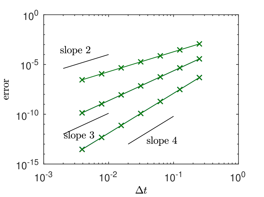
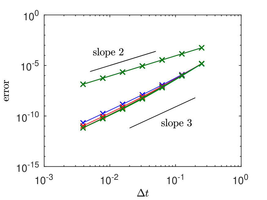
Refer to caption
(a) Micro-macro method.
Refer to caption
(b) Pullback method.
Figure 1: Hénon-Heiles model. Error as a function of ΔtΔ𝑡\Delta t for ε=2k𝜀superscript2𝑘\varepsilon=2^{-k}, k{0,1,2,,9}𝑘0129k\in\{0,1,2,\cdots,9\}. Fig. 1(a) (micro-macro method): UA scheme SΔtRK2subscriptsuperscript𝑆𝑅𝐾2Δ𝑡S^{RK2}_{\Delta t} of order 2 (top curves), UA scheme SΔtextrap3subscriptsuperscript𝑆𝑒𝑥𝑡𝑟𝑎𝑝3Δ𝑡S^{extrap3}_{\Delta t} of order 3 (middle curves) and UA scheme SΔtextrap4subscriptsuperscript𝑆𝑒𝑥𝑡𝑟𝑎𝑝4Δ𝑡S^{extrap4}_{\Delta t} of order 4 (bottom curves). Fig. 1(b) (pullback method): UA scheme SΔtmidpointsubscriptsuperscript𝑆𝑚𝑖𝑑𝑝𝑜𝑖𝑛𝑡Δ𝑡S^{midpoint}_{\Delta t} of order 2 (top curves) and UA scheme SΔtcompos3subscriptsuperscript𝑆𝑐𝑜𝑚𝑝𝑜𝑠3Δ𝑡S^{compos3}_{\Delta t} of order 3 (bottom curves).

5.3 The Hénon-Heiles model - pullback method

In this section, we present the results obtained with the pullback method with stroboscopic averaging for the Hénon-Heiles model. In Figure 1(b), we have represented the error at time Tfinal=1subscript𝑇𝑓𝑖𝑛𝑎𝑙1T_{final}=1 as a function of ΔtΔ𝑡\Delta t for different values of ε𝜀\varepsilon, for our UA scheme SΔtmidpointsubscriptsuperscript𝑆𝑚𝑖𝑑𝑝𝑜𝑖𝑛𝑡Δ𝑡S^{midpoint}_{\Delta t} of order 2 and for our UA scheme SΔtcompos3subscriptsuperscript𝑆𝑐𝑜𝑚𝑝𝑜𝑠3Δ𝑡S^{compos3}_{\Delta t} of order 3. These figures confirm that our schemes are UA, as stated by Theorem 3.5. Note that for these schemes, the variable θ𝜃\theta of the vector field Fε,θ[n]subscriptsuperscript𝐹delimited-[]𝑛𝜀𝜃F^{[n]}_{\varepsilon,\theta} is discretized with 32 points and FFT is used to compute all the integrals444This discretization turns out to be exact for the Hénon-Heiles problem, due to the low degree of the involved trigonometric polynomials.. The initial data is (0.12,0.12,0.12,0.12)0.120.120.120.12(0.12,0.12,0.12,0.12).

Let us now check that our schemes constructed on the stroboscopic averaging pullback method have the expected geometric properties. In Figure 2(a), we have represented the evolution of the error on the Hamiltonian H𝐻H for ε=1𝜀1\varepsilon=1 over long times t30000𝑡30000t\leq 30000 for the scheme SΔtmidpointsubscriptsuperscript𝑆𝑚𝑖𝑑𝑝𝑜𝑖𝑛𝑡Δ𝑡S^{midpoint}_{\Delta t} with Δt=0.1Δ𝑡0.1\Delta t=0.1 and Δt=0.2Δ𝑡0.2\Delta t=0.2 and for the scheme SΔtcompos3subscriptsuperscript𝑆𝑐𝑜𝑚𝑝𝑜𝑠3Δ𝑡S^{compos3}_{\Delta t} with Δt=0.2Δ𝑡0.2\Delta t=0.2. In Figure 2(b), we have represented the results of the same calculations with ε=0.001𝜀0.001\varepsilon=0.001. The initial data is (0,0,p1,p2)00subscript𝑝1subscript𝑝2(0,0,p_{1},p_{2}) with p1=2ε/12sin(π8)subscript𝑝12𝜀12𝜋8p_{1}=\sqrt{2\varepsilon/12}\sin(\frac{\pi}{8}), p2=2/12cos(π8)subscript𝑝2212𝜋8p_{2}=\sqrt{2/12}\cos(\frac{\pi}{8}). We observe no drift for the Hamiltonian.
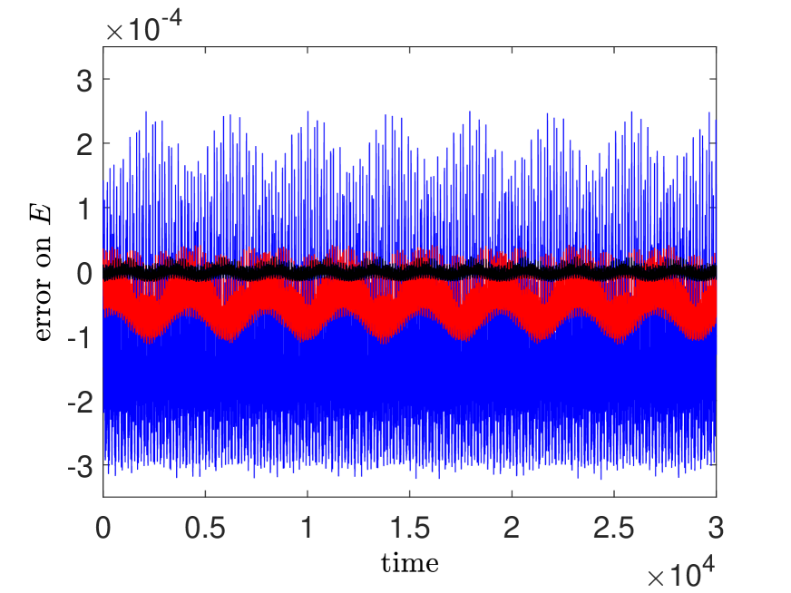
Refer to caption
(a) ε=1𝜀1\varepsilon=1.
Refer to caption
(b) ε=0.001𝜀0.001\varepsilon=0.001.
Figure 2: Hénon-Heiles model, pullback method. Long time evolution of the error on the Hamiltonian. UA scheme SΔtmidpointsubscriptsuperscript𝑆𝑚𝑖𝑑𝑝𝑜𝑖𝑛𝑡Δ𝑡S^{midpoint}_{\Delta t} of order 2 (blue: Δt=0.2Δ𝑡0.2\Delta t=0.2; red: Δt=0.1Δ𝑡0.1\Delta t=0.1). UA scheme SΔtcompos3subscriptsuperscript𝑆𝑐𝑜𝑚𝑝𝑜𝑠3Δ𝑡S^{compos3}_{\Delta t} of order 3 (black: Δt=0.2Δ𝑡0.2\Delta t=0.2).

Let us now observe the so-called Poincaré cuts [14, 13], i.e. the points (q2,p2)subscript𝑞2subscript𝑝2(q_{2},p_{2}) reached when the solution crosses the hyperplane q1=0subscript𝑞10q_{1}=0 with p1>0subscript𝑝10p_{1}>0.

In Figure 3(a), we have represented 5 orbits for ε=1𝜀1\varepsilon=1, 0t300000𝑡300000\leq t\leq 30000 and for the energy H=1/12𝐻112H=1/12. The initial data are (0,0,p1,p2)00subscript𝑝1subscript𝑝2(0,0,p_{1},p_{2}) with p1=2εHsin(θπ2)subscript𝑝12𝜀𝐻𝜃𝜋2p_{1}=\sqrt{2\varepsilon H}\sin(\theta\frac{\pi}{2}), p2=2Hcos(θπ2)subscript𝑝22𝐻𝜃𝜋2p_{2}=\sqrt{2H}\cos(\theta\frac{\pi}{2}) with θ=0.025, 0.25, 0.75, 0.95𝜃0.0250.250.750.95\theta=0.025,\,0.25,\,0.75,\,0.95 and 1.251.251.25. Our UA scheme SΔtmidpointsubscriptsuperscript𝑆𝑚𝑖𝑑𝑝𝑜𝑖𝑛𝑡Δ𝑡S^{midpoint}_{\Delta t} is used with the timestep Δt=0.1Δ𝑡0.1\Delta t=0.1 for t30000𝑡30000t\leq 30000.

In Figure 3(b), we have represented 3 orbits for ε=0.001𝜀0.001\varepsilon=0.001, 0t300000𝑡300000\leq t\leq 30000 and for the energy H=1/6𝐻16H=1/6. The initial data are (0,0,p1,p2)00subscript𝑝1subscript𝑝2(0,0,p_{1},p_{2}) with p1=2εHsin(θπ2)subscript𝑝12𝜀𝐻𝜃𝜋2p_{1}=\sqrt{2\varepsilon H}\sin(\theta\frac{\pi}{2}), p2=2Hcos(θπ2)subscript𝑝22𝐻𝜃𝜋2p_{2}=\sqrt{2H}\cos(\theta\frac{\pi}{2}) with θ=0.1, 0.5𝜃0.10.5\theta=0.1,\,0.5 and 0.90.90.9. Our UA scheme SΔtmidpointsubscriptsuperscript𝑆𝑚𝑖𝑑𝑝𝑜𝑖𝑛𝑡Δ𝑡S^{midpoint}_{\Delta t} is used with the timestep Δt=0.1Δ𝑡0.1\Delta t=0.1 for t30000𝑡30000t\leq 30000.

On these two figures, we observe that the Poincaré curves are well reproduced, which indicate that the ”formal second invariant” is well preserved by our scheme.
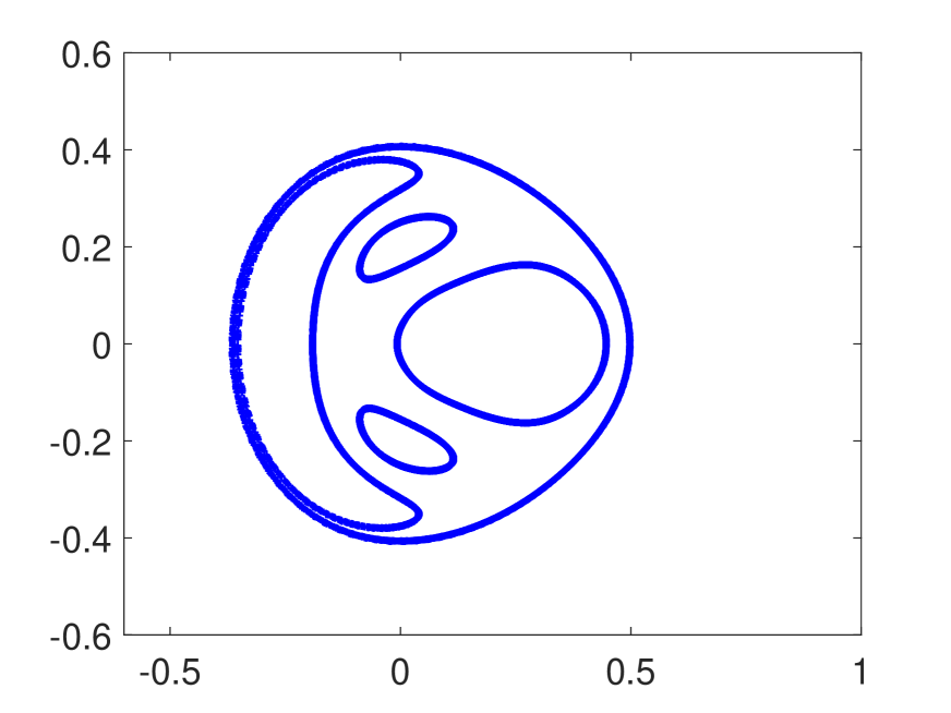
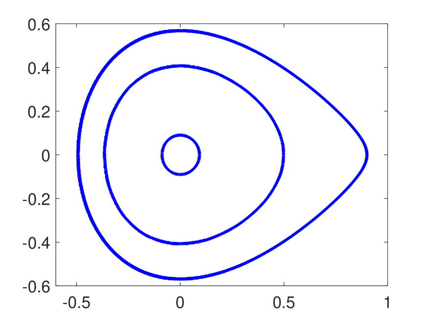
Refer to caption
(a) ε=1𝜀1\varepsilon=1, H=1/12𝐻112H=1/12.
Refer to caption
(b) ε=0.001𝜀0.001\varepsilon=0.001, H=1/6𝐻16H=1/6.
Figure 3: Poincaré cuts for the Hénon-Heiles model. Pullback method with SΔtmidpointsubscriptsuperscript𝑆𝑚𝑖𝑑𝑝𝑜𝑖𝑛𝑡Δ𝑡S^{midpoint}_{\Delta t}.

5.4 The nonlinear Klein-Gordon equation in the nonrelativistic limit regime - micro-macro method

We consider the nonlinear Klein-Gordon (NKG) equation in the nonrelativistic limit regime, also studied numerically in [1, 2, 5, 12]:

εttuΔu+1εu+f(u)=0,xd,t>0,formulae-sequence𝜀subscript𝑡𝑡𝑢Δ𝑢1𝜀𝑢𝑓𝑢0formulae-sequence𝑥superscript𝑑𝑡0\varepsilon\partial_{tt}u-\Delta u+\frac{1}{\varepsilon}u+f(u)=0,\qquad x\in{\mathbb{R}}^{d},\quad t>0, (5.3)

with initial conditions given as

u(0,x)=ϕ(x),tu(0,x)=1εγ(x),xd.formulae-sequence𝑢0𝑥italic-ϕ𝑥formulae-sequencesubscript𝑡𝑢0𝑥1𝜀𝛾𝑥𝑥superscript𝑑u(0,x)=\phi(x),\qquad\partial_{t}u(0,x)=\frac{1}{\varepsilon}\gamma(x),\qquad x\in{\mathbb{R}}^{d}. (5.4)

The unknown is the function u(t,x):1+d:𝑢𝑡𝑥superscript1𝑑u(t,x):\,{\mathbb{R}}^{1+d}\to{\mathbb{C}} and the parameter ε>0𝜀0\varepsilon>0 is inversely proportional to the square of the speed of light. In our simulations, we take d=1𝑑1d=1 and the nonlinearity is f(u)=4|u|2u𝑓𝑢4superscript𝑢2𝑢f(u)=4|u|^{2}u. The limit ε0𝜀0\varepsilon\to 0 in equation (5.3), (5.4), referred to as the nonrelativistic limit, has been studied in [15, 16, 17].

It is convenient to rewrite (5.3) under the equivalent form of a first order system in time (see e.g. [17]). Setting

v+=uiε(1εΔ)1/2tu,v=u¯iε(1εΔ)1/2tu¯,formulae-sequencesubscript𝑣𝑢𝑖𝜀superscript1𝜀Δ12subscript𝑡𝑢subscript𝑣¯𝑢𝑖𝜀superscript1𝜀Δ12subscript𝑡¯𝑢v_{+}=u-i\varepsilon(1-\varepsilon\Delta)^{-1/2}\partial_{t}u,\qquad v_{-}=\overline{u}-i\varepsilon(1-\varepsilon\Delta)^{-1/2}\partial_{t}\overline{u}, (5.5)

and denoting

f±(v)=f(12(v±+v¯)),subscript𝑓plus-or-minus𝑣𝑓12subscript𝑣plus-or-minus¯subscript𝑣minus-or-plusf_{\pm}(v)=f\left(\frac{1}{2}(v_{\pm}+\overline{v_{\mp}})\right),

we obtain that (5.3), (5.4) is equivalent to the following system on the unknown v=(v+,v)𝑣subscript𝑣subscript𝑣v=(v_{+},v_{-}):

itv±=1ε(1εΔ)1/2v±(1εΔ)1/2f±(v),𝑖subscript𝑡subscript𝑣plus-or-minus1𝜀superscript1𝜀Δ12subscript𝑣plus-or-minussuperscript1𝜀Δ12subscript𝑓plus-or-minus𝑣i\partial_{t}v_{\pm}=-\frac{1}{\varepsilon}(1-\varepsilon\Delta)^{1/2}v_{\pm}-(1-\varepsilon\Delta)^{-1/2}f_{\pm}(v), (5.6)
v(0,)=(v+(0,),v(0,))=(ϕi(1εΔ)1/2γ,ϕ¯i(1εΔ)1/2γ¯).𝑣0subscript𝑣0subscript𝑣0italic-ϕ𝑖superscript1𝜀Δ12𝛾¯italic-ϕ𝑖superscript1𝜀Δ12¯𝛾v(0,\cdot)=(v_{+}(0,\cdot),v_{-}(0,\cdot))=\left(\phi-i(1-\varepsilon\Delta)^{-1/2}\gamma\,,\,\overline{\phi}-i(1-\varepsilon\Delta)^{-1/2}\overline{\gamma}\right). (5.7)

Let us introduce the filtered unknowns

v~±=eitε1εΔv±.subscript~𝑣plus-or-minussuperscript𝑒𝑖𝑡𝜀1𝜀Δsubscript𝑣plus-or-minus\widetilde{v}_{\pm}=e^{-i\frac{t}{\varepsilon}\sqrt{1-\varepsilon\Delta}}v_{\pm}.

These quantities satisfy the following equation:

tv~±=i(1εΔ)1/2eitε1εΔf±(eitε1εΔv~).subscript𝑡subscript~𝑣plus-or-minus𝑖superscript1𝜀Δ12superscript𝑒𝑖𝑡𝜀1𝜀Δsubscript𝑓plus-or-minussuperscript𝑒𝑖𝑡𝜀1𝜀Δ~𝑣\partial_{t}\widetilde{v}_{\pm}=i(1-\varepsilon\Delta)^{-1/2}e^{-i\frac{t}{\varepsilon}\sqrt{1-\varepsilon\Delta}}f_{\pm}\left(e^{i\frac{t}{\varepsilon}\sqrt{1-\varepsilon\Delta}}\widetilde{v}\right). (5.8)

Note that (5.8) is under the form

tv~±(t)=f±(tε,t,v~(t)),subscript𝑡subscript~𝑣plus-or-minus𝑡subscript𝑓plus-or-minus𝑡𝜀𝑡~𝑣𝑡\partial_{t}\widetilde{v}_{\pm}(t)=f_{\pm}\left(\frac{t}{\varepsilon},t,\widetilde{v}(t)\right),

if we set

f±(θ,t,u)=i(1εΔ)1/2eiθeitAεf±(eiθeitAεu)subscript𝑓plus-or-minus𝜃𝑡𝑢𝑖superscript1𝜀Δ12superscript𝑒𝑖𝜃superscript𝑒𝑖𝑡subscript𝐴𝜀subscript𝑓plus-or-minussuperscript𝑒𝑖𝜃superscript𝑒𝑖𝑡subscript𝐴𝜀𝑢f_{\pm}(\theta,t,u)=i(1-\varepsilon\Delta)^{-1/2}e^{-i\theta}e^{-itA_{\varepsilon}}f_{\pm}\left(e^{i\theta}e^{itA_{\varepsilon}}u\right) (5.9)

with

Aε=1ε(1εΔ1).subscript𝐴𝜀1𝜀1𝜀Δ1A_{\varepsilon}=\frac{1}{\varepsilon}\left(\sqrt{1-\varepsilon\Delta}-1\right).

The system has two natural invariants:

  • the conserved charge (quadratic invariant)

    Q=Imdεu˙u¯𝑑x𝑄Imsubscriptsuperscript𝑑𝜀˙𝑢¯𝑢differential-d𝑥\displaystyle Q=\operatorname{Im}\int_{{\mathbb{R}}^{d}}\varepsilon\dot{u}\,\overline{u}\,dx =14d(1εΔ)1/2v+v+¯𝑑x14d(1εΔ)1/2vv¯𝑑xabsent14subscriptsuperscript𝑑superscript1𝜀Δ12subscript𝑣¯subscript𝑣differential-d𝑥14subscriptsuperscript𝑑superscript1𝜀Δ12subscript𝑣¯subscript𝑣differential-d𝑥\displaystyle=\frac{1}{4}\int_{{\mathbb{R}}^{d}}(1-\varepsilon\Delta)^{1/2}v_{+}\,\overline{v_{+}}\,dx-\frac{1}{4}\int_{{\mathbb{R}}^{d}}(1-\varepsilon\Delta)^{1/2}v_{-}\,\overline{v_{-}}\,dx
    =14d(1εΔ)1/2v~+v~+¯𝑑x14d(1εΔ)1/2v~v~¯𝑑xabsent14subscriptsuperscript𝑑superscript1𝜀Δ12subscript~𝑣¯subscript~𝑣differential-d𝑥14subscriptsuperscript𝑑superscript1𝜀Δ12subscript~𝑣¯subscript~𝑣differential-d𝑥\displaystyle=\frac{1}{4}\int_{{\mathbb{R}}^{d}}(1-\varepsilon\Delta)^{1/2}\widetilde{v}_{+}\,\overline{\widetilde{v}_{+}}\,dx-\frac{1}{4}\int_{{\mathbb{R}}^{d}}(1-\varepsilon\Delta)^{1/2}\widetilde{v}_{-}\,\overline{\widetilde{v}_{-}}\,dx
  • the energy

    E=εd|u˙|2𝑑x+d|u|2𝑑x+1εd|u|2𝑑x+2d|u|4𝑑x.𝐸𝜀subscriptsuperscript𝑑superscript˙𝑢2differential-d𝑥subscriptsuperscript𝑑superscript𝑢2differential-d𝑥1𝜀subscriptsuperscript𝑑superscript𝑢2differential-d𝑥2subscriptsuperscript𝑑superscript𝑢4differential-d𝑥E=\varepsilon\int_{{\mathbb{R}}^{d}}|\dot{u}|^{2}\,dx+\int_{{\mathbb{R}}^{d}}|\nabla u|^{2}\,dx+\frac{1}{\varepsilon}\int_{{\mathbb{R}}^{d}}|u|^{2}\,dx+2\int_{{\mathbb{R}}^{d}}|u|^{4}\,dx.

In the simulations of this subsection, we take the following initial data:

ϕ(x)=12cosx,γ(x)=12sinx.formulae-sequenceitalic-ϕ𝑥12𝑥𝛾𝑥12𝑥\phi(x)=\frac{1}{2-\cos x},\qquad\gamma(x)=\frac{1}{2-\sin x}. (5.10)

For Figure 4(a), the final time of the simulations is Tfinal=0.25subscript𝑇𝑓𝑖𝑛𝑎𝑙0.25T_{final}=0.25. The computational domain in x𝑥x is [0,2π]02𝜋[0,2\pi]. For the numerical evaluations of the function f𝑓f in our scheme, a spectral method is used in the x𝑥x variable and the fast Fourier transform is used in the practical implementation. For these tests, the reference solution is computed by our third order UA method SΔtextrap3subscriptsuperscript𝑆𝑒𝑥𝑡𝑟𝑎𝑝3Δ𝑡S^{extrap3}_{\Delta t} applied to the standard averaging micro-macro method with 256 grid points in x𝑥x, 128 grid points in θ𝜃\theta and Δt=Tfinal/4096Δ𝑡subscript𝑇𝑓𝑖𝑛𝑎𝑙4096\Delta t=T_{final}/4096. We use the H1superscript𝐻1H^{1} relative error of a given numerical scheme which we define as

1=uref(Tfinal,)unum(Tfinal,)H1uref(Tfinal,)H1,subscript1subscriptnormsuperscript𝑢𝑟𝑒𝑓subscript𝑇𝑓𝑖𝑛𝑎𝑙superscript𝑢𝑛𝑢𝑚subscript𝑇𝑓𝑖𝑛𝑎𝑙superscript𝐻1subscriptnormsuperscript𝑢𝑟𝑒𝑓subscript𝑇𝑓𝑖𝑛𝑎𝑙superscript𝐻1{\mathcal{E}}_{1}=\frac{\|u^{ref}(T_{final},\cdot)-u^{num}(T_{final},\cdot)\|_{H^{1}}}{\|u^{ref}(T_{final},\cdot)\|_{H^{1}}}, (5.11)

where unum(tfinal,)superscript𝑢𝑛𝑢𝑚subscript𝑡𝑓𝑖𝑛𝑎𝑙u^{num}(t_{final},\cdot) is the approximated solution obtained by the considered numerical scheme, at the final time Tfinalsubscript𝑇𝑓𝑖𝑛𝑎𝑙T_{final} of the simulation.

Let us present the results for the standard averaging micro-macro method. In this case, the analytic computation of the integrals in θ𝜃\theta involves a too heavy system of equations and it is more convenient to compute these integrals numerically at each iteration of the scheme, by using fast Fourier transform techniques. In Figure 4(a), we have represented the error at Tfinal=0.25subscript𝑇𝑓𝑖𝑛𝑎𝑙0.25T_{final}=0.25 as a function of ΔtΔ𝑡\Delta t, for different values of ε𝜀\varepsilon, for our UA scheme SΔtRK2subscriptsuperscript𝑆𝑅𝐾2Δ𝑡S^{RK2}_{\Delta t} of order 2, for our UA scheme SΔtextrap3subscriptsuperscript𝑆𝑒𝑥𝑡𝑟𝑎𝑝3Δ𝑡S^{extrap3}_{\Delta t} of order 3 and for our UA scheme SΔtextrap4subscriptsuperscript𝑆𝑒𝑥𝑡𝑟𝑎𝑝4Δ𝑡S^{extrap4}_{\Delta t} of order 4. These curves confirm that the schemes are UA respectively of order 2, 3 and 4. The numerical parameters are the following: we have taken 128 discretization points in the x𝑥x variable and 646464 discretization points in θ𝜃\theta for the quadrature methods.

Refer to caption
(a) Micro-macro method.
Refer to caption
(b) Pullback method.
Figure 4: NKG model. Error as a function of ΔtΔ𝑡\Delta t for ε{1,101,102,103,104,105,106}𝜀1superscript101superscript102superscript103superscript104superscript105superscript106\varepsilon\in\{1,10^{-1},10^{-2},10^{-3},10^{-4},10^{-5},10^{-6}\}. Fig. 4(a) (micro-macro method): UA scheme SΔtRK2subscriptsuperscript𝑆𝑅𝐾2Δ𝑡S^{RK2}_{\Delta t} of order 2 (top curves), UA scheme SΔtextrap3subscriptsuperscript𝑆𝑒𝑥𝑡𝑟𝑎𝑝3Δ𝑡S^{extrap3}_{\Delta t} of order 3 (middle curves) and UA scheme SΔtextrap4subscriptsuperscript𝑆𝑒𝑥𝑡𝑟𝑎𝑝4Δ𝑡S^{extrap4}_{\Delta t} of order 4 (bottom curves). Fig. 4(b) (pullback method): scheme SΔtmidpointsubscriptsuperscript𝑆𝑚𝑖𝑑𝑝𝑜𝑖𝑛𝑡Δ𝑡S^{midpoint}_{\Delta t} of order 2 (top curves) and scheme SΔtcompos3subscriptsuperscript𝑆𝑐𝑜𝑚𝑝𝑜𝑠3Δ𝑡S^{compos3}_{\Delta t} of order 3 (bottom curves).

5.5 The nonlinear Klein-Gordon equation in the nonrelativistic limit regime - pullback method

We now present the results of the pullback method with the schemes SΔtmidpointsubscriptsuperscript𝑆𝑚𝑖𝑑𝑝𝑜𝑖𝑛𝑡Δ𝑡S^{midpoint}_{\Delta t} and SΔtcompos3subscriptsuperscript𝑆𝑐𝑜𝑚𝑝𝑜𝑠3Δ𝑡S^{compos3}_{\Delta t}. In Figure 4(b), we have plotted the error as a function of ΔtΔ𝑡\Delta t for different values of ε𝜀\varepsilon. For this figure, we have discretized the θ𝜃\theta variable with 646464 points and the x𝑥x variable with 128128128 points, the initial data is (5.10) and the final time of the simulation is Tfinal=0.25subscript𝑇𝑓𝑖𝑛𝑎𝑙0.25T_{final}=0.25. These numerical experiments confirm that our schemes SΔtmidpointsubscriptsuperscript𝑆𝑚𝑖𝑑𝑝𝑜𝑖𝑛𝑡Δ𝑡S^{midpoint}_{\Delta t} and SΔtcompos3subscriptsuperscript𝑆𝑐𝑜𝑚𝑝𝑜𝑠3Δ𝑡S^{compos3}_{\Delta t} are respectively UA of order 2 and 3.

In Figure 5(a), we have represented the long time (t1000𝑡1000t\leq 1000) conservation of the quadratic invariant Q𝑄Q for our two schemes SΔtmidpointsubscriptsuperscript𝑆𝑚𝑖𝑑𝑝𝑜𝑖𝑛𝑡Δ𝑡S^{midpoint}_{\Delta t} and SΔtcompos3subscriptsuperscript𝑆𝑐𝑜𝑚𝑝𝑜𝑠3Δ𝑡S^{compos3}_{\Delta t} and in Figure 5(b) we have plotted the evolution of the relative error on the energy. The maximal absolute value of the error on E𝐸E is 108superscript10810^{-8} for the second order scheme and is 2×10102superscript10102\times 10^{-10} for the third order scheme. The initial data, with a non trivial value of Q𝑄Q, is

ϕ(x)=(1+i)(cosx+sinx),γ(x)=(1i/2)cosx+(1/2+i)sinx.formulae-sequenceitalic-ϕ𝑥1𝑖𝑥𝑥𝛾𝑥1𝑖2𝑥12𝑖𝑥\phi(x)=(1+i)(\cos x+\sin x),\qquad\gamma(x)=(1-i/2)\cos x+(1/2+i)\sin x.

The blue curves correspond to SΔtmidpointsubscriptsuperscript𝑆𝑚𝑖𝑑𝑝𝑜𝑖𝑛𝑡Δ𝑡S^{midpoint}_{\Delta t} with Δt=0.01Δ𝑡0.01\Delta t=0.01 and the red curves correspond to SΔtcompos3subscriptsuperscript𝑆𝑐𝑜𝑚𝑝𝑜𝑠3Δ𝑡S^{compos3}_{\Delta t} with Δt=0.01Δ𝑡0.01\Delta t=0.01. In all the simulations, we have ε=0.0001𝜀0.0001\varepsilon=0.0001 and we have taken 64 points for the discretization of the x𝑥x variable as well as for the θ𝜃\theta variable. The quadratic invariant Q𝑄Q is an exact invariant (up to round-off errors) of the two schemes, and we observe no energy drift over long times.
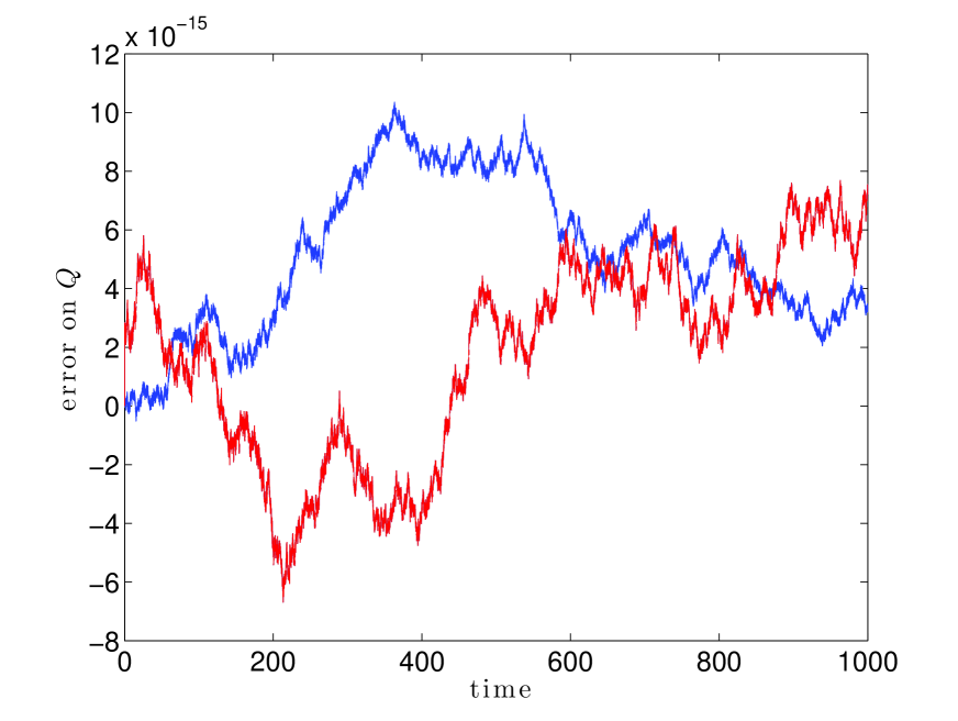
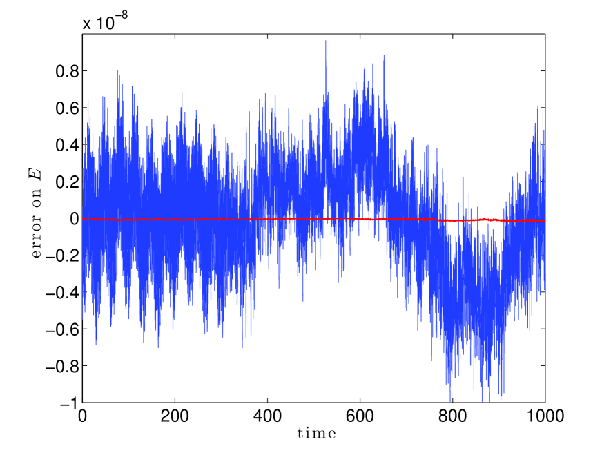
Refer to caption
(a) quadratic invariant error.
Refer to caption
(b) Energy error.
Figure 5: NKG model with ε=104𝜀superscript104\varepsilon=10^{-4}, pullback method. Long-time evolution of the relative error on the quadratic invariant and on the energy. Blue: UA scheme SΔtmidpointsubscriptsuperscript𝑆𝑚𝑖𝑑𝑝𝑜𝑖𝑛𝑡Δ𝑡S^{midpoint}_{\Delta t} with Δt=0.01Δ𝑡0.01\Delta t=0.01. Red: UA scheme SΔtcompos3subscriptsuperscript𝑆𝑐𝑜𝑚𝑝𝑜𝑠3Δ𝑡S^{compos3}_{\Delta t} with Δt=0.01Δ𝑡0.01\Delta t=0.01.

6 Conclusion

We have shown that by transforming the original problem (1.1) through a change of variables inspired from the theory of averaging, it becomes possible to apply standard nonstiff numerical schemes (i.e. integrators which would properly solve equation (1.1) with ε=1𝜀1\varepsilon=1) for all values of ε]0,1]\varepsilon\in]0,1] with a computational cost and accuracy both independent of ε]0,1]\varepsilon\in]0,1]. This has been done in four different ways whose merits have been discussed in details. Roughly speaking, stroboscopic averaging used in conjunction with the pullback method leads to geometric uniformly accurate integrators while standard averaging associated with a micro-macro decomposition leads to comparatively cheap uniformly accurate methods (which are not geometric though). As far as efficiency is concerned, the most relevant question is to estimate the critical threshold value εcsubscript𝜀𝑐\varepsilon_{c} below which our techniques become superior to standard schemes. Although such an εcsubscript𝜀𝑐\varepsilon_{c} clearly always exists, it is delicate to estimate its value as it strongly depends on the problem itself and on the choices of implementation made in the various methods: for instance, we have exploited here the fact that both the change of variable and the averaged vector field can be computed at first and second orders exactly for the Henon-Heiles problem. Whenever this is possible, most of the additional formulae required by our techniques can be pre-computed, making the formers indeed very competitive even for large values of ε𝜀\varepsilon (i.e. εcsubscript𝜀𝑐\varepsilon_{c} is relatively large). The situation is different when this option is precluded (e.g. for the Klein-Gordon equation) and in that case the value of εcsubscript𝜀𝑐\varepsilon_{c} is undoubtedly smaller. However, we wish to emphasize that whatever its value might be, our technique remains of interest for variants of the model equation (1.1) where ε𝜀\varepsilon may undergo large variations.

Acknowledgements. This work was partially supported by the Swiss National Science Foundation, grants No: 200020_144313/1 and 200021_162404 and by the ANR project Moonrise ANR-14-CE23-0007-01.

Appendix

This section is devoted to the proof of Proposition 3.2 and Theorem 3.3. We first recall the two following basic results from [4]:

Lemma A.1 (See Castella, Chartier, Murua and Méhats [4]).

Let 0<δ<ρ2R0𝛿𝜌2𝑅0<\delta<\rho\leq 2R. Assume that the function (θ,u)𝕋×𝒦ρφθ(u)X𝜃𝑢𝕋subscript𝒦𝜌maps-tosubscript𝜑𝜃𝑢subscript𝑋(\theta,u)\in\mathbb{T}\times{\cal K}_{\rho}\mapsto\varphi_{\theta}(u)\in X_{\mathbb{C}} is analytic, and that φθsubscript𝜑𝜃\varphi_{\theta} is a near-identity mapping, in the sense that

φIdρδ2.subscriptnorm𝜑Id𝜌𝛿2\|\varphi-{\rm Id}\|_{\rho}\leq\frac{\delta}{2}.

Then uφρδ32subscriptnormsubscript𝑢𝜑𝜌𝛿32\|\partial_{u}\varphi\|_{\rho-\delta}\leq\frac{3}{2}, the mapping uφ1subscript𝑢superscriptdelimited-⟨⟩𝜑1\partial_{u}\langle\varphi\rangle^{-1} is well-defined and analytic on 𝒦ρδsubscript𝒦𝜌𝛿{\cal K}_{\rho-\delta} with uφ1ρδ2subscriptnormsubscript𝑢superscriptdelimited-⟨⟩𝜑1𝜌𝛿2\|\partial_{u}\langle\varphi\rangle^{-1}\|_{\rho-\delta}\leq 2, and the mappings (θ,u)𝕋×𝒦ρδΛ(φ)θ(u)𝜃𝑢𝕋subscript𝒦𝜌𝛿maps-toΛsubscript𝜑𝜃𝑢(\theta,u)\in\mathbb{T}\times{\cal K}_{\rho-\delta}\mapsto\Lambda(\varphi)_{\theta}(u) and (θ,u)𝕋×KρδΓε(φ)θ(u)𝜃𝑢𝕋subscript𝐾𝜌𝛿maps-tosuperscriptΓ𝜀subscript𝜑𝜃𝑢(\theta,u)\in\mathbb{T}\times K_{\rho-\delta}\mapsto\Gamma^{\varepsilon}(\varphi)_{\theta}(u) are well-defined and analytic. In addition, the following bounds hold for all ε0𝜀0\varepsilon\geq 0,

Λ(φ)ρδ4M and Γε(φ)Idρδ4Mε.formulae-sequencesubscriptnormΛ𝜑𝜌𝛿4𝑀 and subscriptnormsuperscriptΓ𝜀𝜑Id𝜌𝛿4𝑀𝜀\|\Lambda(\varphi)\|_{\rho-\delta}\leq 4\,M\quad\mbox{ and }\quad\|\Gamma^{\varepsilon}(\varphi)-{\rm Id}\|_{\rho-\delta}\leq 4\,M\,\varepsilon.

Lemma A.1 shows that, starting from a function (θ,u)𝕋×𝒦2Rφθ(u)X𝜃𝑢𝕋subscript𝒦2𝑅maps-tosubscript𝜑𝜃𝑢subscript𝑋(\theta,u)\in\mathbb{T}\times{\cal K}_{2R}\mapsto\varphi_{\theta}(u)\in X_{\mathbb{C}}, we can consider iterates (Γε)k(φ)θsuperscriptsuperscriptΓ𝜀𝑘subscript𝜑𝜃\left(\Gamma^{\varepsilon}\right)^{k}(\varphi)_{\theta} at the cost of a gradual thinning of their domains of analyticity. The following contraction property holds.

Lemma A.2 (See Castella, Chartier, Murua and Méhats [4]).

Let 0<δ<ρ2R0𝛿𝜌2𝑅0<\delta<\rho\leq 2R and consider two periodic, near-identity mappings (θ,u)𝕋×𝒦ρφθ(u)𝜃𝑢𝕋subscript𝒦𝜌maps-tosubscript𝜑𝜃𝑢(\theta,u)\in\mathbb{T}\times{\cal K}_{\rho}\mapsto\varphi_{\theta}(u) and (θ,u)𝕋×𝒦ρφ~θ(u)𝜃𝑢𝕋subscript𝒦𝜌maps-tosubscript~𝜑𝜃𝑢(\theta,u)\in\mathbb{T}\times{\cal K}_{\rho}\mapsto\tilde{\varphi}_{\theta}(u), analytic on 𝒦ρsubscript𝒦𝜌{\cal K}_{\rho} and satisfying

φIdρδ2andφ~Idρδ2.formulae-sequencesubscriptnorm𝜑Id𝜌𝛿2andsubscriptnorm~𝜑Id𝜌𝛿2\|\varphi-{\rm Id}\|_{\rho}\leq\frac{\delta}{2}\quad\mbox{and}\quad\|\tilde{\varphi}-{\rm Id}\|_{\rho}\leq\frac{\delta}{2}.

Then the following estimates hold for all ε0𝜀0\varepsilon\geq 0,

Λ(φ)Λ(φ~)ρδ16Mδφφ~ρandΓε(φ)Γε(φ~)ρδ16Mεδφφ~ρ.formulae-sequencesubscriptnormΛ𝜑Λ~𝜑𝜌𝛿16𝑀𝛿subscriptnorm𝜑~𝜑𝜌andsubscriptnormsuperscriptΓ𝜀𝜑superscriptΓ𝜀~𝜑𝜌𝛿16𝑀𝜀𝛿subscriptnorm𝜑~𝜑𝜌\|\Lambda(\varphi)-\Lambda(\tilde{\varphi})\|_{\rho-\delta}\leq\frac{16\,M}{\delta}\|\varphi-\tilde{\varphi}\|_{\rho}\quad\mbox{and}\quad\|\Gamma^{\varepsilon}(\varphi)-\Gamma^{\varepsilon}(\tilde{\varphi})\|_{\rho-\delta}\leq\frac{16\,M\varepsilon}{\delta}\|\varphi-\tilde{\varphi}\|_{\rho}.
Proof of Proposition 3.2.

We assume that all Φ[k]superscriptΦdelimited-[]𝑘\Phi^{[k]} are defined by (2.4) in the stroboscopic case (all functions G[k]superscript𝐺delimited-[]𝑘G^{[k]} are taken null). The following properties were already proved in [4]:

  • (i)

    the maps Φ[k]superscriptΦdelimited-[]𝑘\Phi^{[k]} and F[k]:=uΦ[k]1fΦ[k]assignsuperscript𝐹delimited-[]𝑘superscriptdelimited-⟨⟩subscript𝑢superscriptΦdelimited-[]𝑘1delimited-⟨⟩𝑓superscriptΦdelimited-[]𝑘F^{[k]}:=\langle\partial_{u}\Phi^{[k]}\rangle^{-1}\langle f\circ\Phi^{[k]}\rangle are well-defined and analytic on KRksubscript𝐾subscript𝑅𝑘K_{R_{k}} for all k=0,,n+1𝑘0𝑛1k=0,\ldots,n+1;

  • (ii)

    the estimates

    Φ[k]idRkrn2,F[k]Rk+12M and Φ[k+1]Φ[k]RC(2(n+1)εε0)k,formulae-sequencesubscriptnormsuperscriptΦdelimited-[]𝑘idsubscript𝑅𝑘subscript𝑟𝑛2subscriptnormsuperscript𝐹delimited-[]𝑘subscript𝑅𝑘12𝑀 and subscriptnormsuperscriptΦdelimited-[]𝑘1superscriptΦdelimited-[]𝑘𝑅𝐶superscript2𝑛1𝜀subscript𝜀0𝑘\displaystyle\left\|\Phi^{[k]}-{\rm id}\right\|_{R_{k}}\leq\frac{r_{n}}{2},\quad\left\|F^{[k]}\right\|_{R_{k+1}}\leq 2M\;\mbox{ and }\;\left\|\Phi^{[k+1]}-\Phi^{[k]}\right\|_{R}\leq C\left(2(n+1)\frac{\varepsilon}{\varepsilon_{0}}\right)^{k},

    hold for some positive constant C𝐶C independent of n𝑛n, k𝑘k and ε𝜀\varepsilon.

From equation (2.4) with G[k+1]0superscript𝐺delimited-[]𝑘10G^{[k+1]}\equiv 0 and Assumption 3.1, it is obvious that Φ[k]superscriptΦdelimited-[]𝑘\Phi^{[k]} is (p+1)𝑝1(p+1)-times continuously differentiable w.r.t. θ𝜃\theta. We have furthermore, for 0kn0𝑘𝑛0\leq k\leq n

θΦθ[k+1]=ε(fθΦθ[k]uΦθ[k]F[k])subscript𝜃subscriptsuperscriptΦdelimited-[]𝑘1𝜃𝜀subscript𝑓𝜃subscriptsuperscriptΦdelimited-[]𝑘𝜃subscript𝑢subscriptsuperscriptΦdelimited-[]𝑘𝜃superscript𝐹delimited-[]𝑘\displaystyle\partial_{\theta}\Phi^{[k+1]}_{\theta}=\varepsilon\left(f_{\theta}\circ\Phi^{[k]}_{\theta}-\partial_{u}\Phi^{[k]}_{\theta}F^{[k]}\right)

so that, by differentiating νp𝜈𝑝\nu\leq p times w.r.t. θ𝜃\theta with the help of the Leibniz and the Faà di Bruno formulae, we obtain

1εθν+1Φθ[k+1]1𝜀subscriptsuperscript𝜈1𝜃subscriptsuperscriptΦdelimited-[]𝑘1𝜃\displaystyle\frac{1}{\varepsilon}\partial^{\nu+1}_{\theta}\Phi^{[k+1]}_{\theta} =θνfθΦθ[k]+q=1ν(νq)𝐢C𝐢q(θνqu|𝐢|fθ)Φθ[k]((θΦθ[k])i1,,(θqΦθ[k])iq)absentsuperscriptsubscript𝜃𝜈subscript𝑓𝜃subscriptsuperscriptΦdelimited-[]𝑘𝜃superscriptsubscript𝑞1𝜈𝜈𝑞subscript𝐢subscriptsuperscript𝐶𝑞𝐢subscriptsuperscript𝜈𝑞𝜃subscriptsuperscript𝐢𝑢subscript𝑓𝜃subscriptsuperscriptΦdelimited-[]𝑘𝜃superscriptsubscript𝜃subscriptsuperscriptΦdelimited-[]𝑘𝜃subscript𝑖1superscriptsubscriptsuperscript𝑞𝜃subscriptsuperscriptΦdelimited-[]𝑘𝜃subscript𝑖𝑞\displaystyle=\partial_{\theta}^{\nu}f_{\theta}\circ\Phi^{[k]}_{\theta}+\sum_{q=1}^{\nu}\left(\hskip-4.30554pt\begin{array}[]{c}\nu\\ q\end{array}\hskip-4.30554pt\right)\sum_{\bf i}C^{q}_{\bf i}(\partial^{\nu-q}_{\theta}\partial^{|{\bf i}|}_{u}f_{\theta})\circ\Phi^{[k]}_{\theta}\left((\partial_{\theta}\Phi^{[k]}_{\theta})^{i_{1}},\ldots,(\partial^{q}_{\theta}\Phi^{[k]}_{\theta})^{i_{q}}\right)
θνuΦθ[k]F[k]superscriptsubscript𝜃𝜈subscript𝑢subscriptsuperscriptΦdelimited-[]𝑘𝜃superscript𝐹delimited-[]𝑘\displaystyle-\partial_{\theta}^{\nu}\partial_{u}\Phi^{[k]}_{\theta}F^{[k]}

where the inner sum runs over multi-indices 𝐢=(i1,,iq)q𝐢subscript𝑖1subscript𝑖𝑞superscript𝑞{\bf i}=(i_{1},\ldots,i_{q})\in\mathbb{N}^{q} such that i1+2i2++qiq=qsubscript𝑖12subscript𝑖2𝑞subscript𝑖𝑞𝑞i_{1}+2i_{2}+\ldots+qi_{q}=q and where |𝐢|=i1++iq𝐢subscript𝑖1subscript𝑖𝑞|{\bf i}|=i_{1}+\ldots+i_{q} and

C𝐢q=q!i1!i2!2!i2iq!q!iq.subscriptsuperscript𝐶𝑞𝐢𝑞subscript𝑖1subscript𝑖2superscript2subscript𝑖2subscript𝑖𝑞superscript𝑞subscript𝑖𝑞C^{q}_{\bf i}=\frac{q!}{i_{1}!i_{2}!2!^{i_{2}}\ldots i_{q}!q!^{i_{q}}}.

Owing to (ii), for u𝒦Rk+1𝑢subscript𝒦subscript𝑅𝑘1u\in{\cal K}_{R_{k+1}}, Φθ[k](u)subscriptsuperscriptΦdelimited-[]𝑘𝜃𝑢\Phi^{[k]}_{\theta}(u) takes its values in 𝒦Rk+1+rn/2subscript𝒦subscript𝑅𝑘1subscript𝑟𝑛2{\cal K}_{R_{k+1}+r_{n}/2}, a set on which θjuifθsuperscriptsubscript𝜃𝑗superscriptsubscript𝑢𝑖subscript𝑓𝜃\partial_{\theta}^{j}\partial_{u}^{i}f_{\theta} is bounded (due to Assumption 3.1 and Cauchy estimates for analytic functions) as follows:

θjuifRk+1+rn/21(2R(Rk+1+rn/2))iM=M(k+12)irni.subscriptnormsuperscriptsubscript𝜃𝑗superscriptsubscript𝑢𝑖𝑓subscript𝑅𝑘1subscript𝑟𝑛21superscript2𝑅subscript𝑅𝑘1subscript𝑟𝑛2𝑖𝑀𝑀superscript𝑘12𝑖superscriptsubscript𝑟𝑛𝑖\left\|\partial_{\theta}^{j}\partial_{u}^{i}f\right\|_{R_{k+1}+r_{n}/2}\leq\frac{1}{(2R-(R_{k+1}+r_{n}/2))^{i}}M=\frac{M}{(k+\frac{1}{2})^{i}r_{n}^{i}}.

Hence, if we denote αk,ν=θνΦ[k]Rk/(εM)subscript𝛼𝑘𝜈subscriptnormsubscriptsuperscript𝜈𝜃superscriptΦdelimited-[]𝑘subscript𝑅𝑘𝜀𝑀\alpha_{k,\nu}=\|\partial^{\nu}_{\theta}\Phi^{[k]}\|_{R_{k}}/(\varepsilon M), for ν1𝜈1\nu\geq 1, then we have

k1,ν1,αk+1,ν+11+2εMαk,νrn+q=1ν(νq)𝐢C𝐢q(εM)|𝐢|αk𝐢rn|𝐢|(k+12)|𝐢|formulae-sequencefor-all𝑘1formulae-sequencefor-all𝜈1subscript𝛼𝑘1𝜈112𝜀𝑀subscript𝛼𝑘𝜈subscript𝑟𝑛superscriptsubscript𝑞1𝜈𝜈𝑞subscript𝐢subscriptsuperscript𝐶𝑞𝐢superscript𝜀𝑀𝐢superscriptsubscript𝛼𝑘𝐢superscriptsubscript𝑟𝑛𝐢superscript𝑘12𝐢\displaystyle\forall k\geq 1,\quad\forall\nu\geq 1,\quad\alpha_{k+1,\nu+1}\leq 1+\frac{2\varepsilon M\alpha_{k,\nu}}{r_{n}}+\sum_{q=1}^{\nu}\left(\hskip-4.30554pt\begin{array}[]{c}\nu\\ q\end{array}\hskip-4.30554pt\right)\sum_{\bf i}C^{q}_{\bf i}\frac{(\varepsilon M)^{|\bf{i}|}\alpha_{k}^{\bf{i}}}{r_{n}^{|\bf i|}(k+\frac{1}{2})^{|\bf i|}}

where we denote αk𝐢=j=1qαk,jijsuperscriptsubscript𝛼𝑘𝐢superscriptsubscriptproduct𝑗1𝑞superscriptsubscript𝛼𝑘𝑗subscript𝑖𝑗\alpha_{k}^{\bf{i}}=\prod_{j=1}^{q}\alpha_{k,j}^{i_{j}} and use that (owing to (ii) and a Cauchy estimate)

uθνΦ[k]F[k]Rk+11rnθνΦ[k]RkF[k]Rk+12MθνΦ[k]Rkrn.subscriptnormsubscript𝑢superscriptsubscript𝜃𝜈superscriptΦdelimited-[]𝑘superscript𝐹delimited-[]𝑘subscript𝑅𝑘11subscript𝑟𝑛subscriptnormsuperscriptsubscript𝜃𝜈superscriptΦdelimited-[]𝑘subscript𝑅𝑘subscriptnormsuperscript𝐹delimited-[]𝑘subscript𝑅𝑘12𝑀subscriptnormsuperscriptsubscript𝜃𝜈superscriptΦdelimited-[]𝑘subscript𝑅𝑘subscript𝑟𝑛\left\|\partial_{u}\partial_{\theta}^{\nu}\Phi^{[k]}\,F^{[k]}\right\|_{R_{k+1}}\leq\frac{1}{r_{n}}\left\|\partial_{\theta}^{\nu}\Phi^{[k]}\right\|_{R_{k}}\left\|F^{[k]}\right\|_{R_{k+1}}\leq\frac{2M\left\|\partial_{\theta}^{\nu}\Phi^{[k]}\right\|_{R_{k}}}{r_{n}}.

Finally, the assumption that (n+1)εε0=R8M𝑛1𝜀subscript𝜀0𝑅8𝑀(n+1)\varepsilon\leq\varepsilon_{0}=\frac{R}{8M} leads to the inequality

αk+1,ν+11+αk,ν4+q=1ν(νq)𝐢C𝐢qαk𝐢(8k+4)|𝐢|.subscript𝛼𝑘1𝜈11subscript𝛼𝑘𝜈4superscriptsubscript𝑞1𝜈𝜈𝑞subscript𝐢subscriptsuperscript𝐶𝑞𝐢superscriptsubscript𝛼𝑘𝐢superscript8𝑘4𝐢\displaystyle\alpha_{k+1,\nu+1}\leq 1+\frac{\alpha_{k,\nu}}{4}+\sum_{q=1}^{\nu}\left(\hskip-4.30554pt\begin{array}[]{c}\nu\\ q\end{array}\hskip-4.30554pt\right)\sum_{\bf i}C^{q}_{\bf i}\frac{\alpha_{k}^{\bf{i}}}{(8k+4)^{|\bf i|}}. (A.3)

We now introduce the generating functions for ξ𝜉\xi\in\mathbb{C},

gk(ξ)=ν1αk,νξνν!,k=1,formulae-sequencesubscript𝑔𝑘𝜉subscript𝜈1subscript𝛼𝑘𝜈superscript𝜉𝜈𝜈𝑘1g_{k}(\xi)=\sum_{\nu\geq 1}\alpha_{k,\nu}\frac{\xi^{\nu}}{\nu!},\quad k=1,\ldots

A direct estimation gives α1,12subscript𝛼112\alpha_{1,1}\leq 2 and α1,ν1subscript𝛼1𝜈1\alpha_{1,\nu}\leq 1 for ν2𝜈2\nu\geq 2, so that 0g1(ξ)ξ+eξ10subscript𝑔1𝜉𝜉superscript𝑒𝜉10\leq g_{1}(\xi)\leq\xi+e^{\xi}-1 for all ξ+𝜉subscript\xi\in\mathbb{R}_{+} and from (A.3), we obtain (owing to the Leibniz and the Faà di Bruno formulae)

αk+1,ν+1αk,ν4+q=0ν(νq)dqdξqexp(gk(ξ)8k+4)|ξ=0=αk,ν4+Gk(ν)(0)subscript𝛼𝑘1𝜈1subscript𝛼𝑘𝜈4evaluated-atsuperscriptsubscript𝑞0𝜈𝜈𝑞superscript𝑑𝑞𝑑superscript𝜉𝑞subscript𝑔𝑘𝜉8𝑘4𝜉0subscript𝛼𝑘𝜈4subscriptsuperscript𝐺𝜈𝑘0\displaystyle\alpha_{k+1,\nu+1}\leq\frac{\alpha_{k,\nu}}{4}+\sum_{q=0}^{\nu}\left(\hskip-4.30554pt\begin{array}[]{c}\nu\\ q\end{array}\hskip-4.30554pt\right)\left.\frac{d^{q}}{d\xi^{q}}\exp\left(\frac{g_{k}(\xi)}{8k+4}\right)\right|_{\xi=0}=\frac{\alpha_{k,\nu}}{4}+G^{(\nu)}_{k}(0)

where

Gk(ξ)=exp(ξ+gk(ξ)8k+4)subscript𝐺𝑘𝜉𝜉subscript𝑔𝑘𝜉8𝑘4G_{k}(\xi)=\exp\left(\xi+\frac{g_{k}(\xi)}{8k+4}\right)

so that, using αk+1,14subscript𝛼𝑘114\alpha_{k+1,1}\leq 4, we have for ξ+𝜉subscript\xi\in\mathbb{R}_{+}

gk+1(ξ)3ξ+140ξgk(s)ds+0ξGk(s)ds.subscript𝑔𝑘1𝜉3𝜉14superscriptsubscript0𝜉subscript𝑔𝑘sdssuperscriptsubscript0𝜉subscriptGksdsg_{k+1}(\xi)\leq 3\xi+\frac{1}{4}\int_{0}^{\xi}g_{k}(\rm s)ds+\int_{0}^{\xi}G_{k}(s)ds.

Noticing that sup0ξ1gk(ξ)=gk(1)subscriptsupremum0𝜉1subscript𝑔𝑘𝜉subscript𝑔𝑘1\sup_{0\leq\xi\leq 1}g_{k}(\xi)=g_{k}(1), the previous inequality leads to

gk+1(1)3+14gk(1)+(e1)exp(gk(1)8k+4)subscript𝑔𝑘11314subscript𝑔𝑘1𝑒1subscript𝑔𝑘18𝑘4g_{k+1}(1)\leq 3+\frac{1}{4}g_{k}(1)+(e-1)\exp\left(\frac{g_{k}(1)}{8k+4}\right)

and an easy induction shows that the sequence (gk(1))k1subscriptsubscript𝑔𝑘1𝑘1(g_{k}(1))_{k\geq 1} is upper-bounded by 888. We conclude the proof by applying Cauchy estimates as follows:

1kn+1,1νp+1,αk,ν=|dνgkdξν(0)|ν!sup|ξ|1|gk(ξ)|1νν!gk(1)8ν!formulae-sequencefor-all1𝑘𝑛1for-all1𝜈𝑝1subscript𝛼𝑘𝜈superscript𝑑𝜈subscript𝑔𝑘𝑑superscript𝜉𝜈0𝜈subscriptsupremum𝜉1subscript𝑔𝑘𝜉superscript1𝜈𝜈subscript𝑔𝑘18𝜈\forall 1\leq k\leq n+1,\,\forall 1\leq\nu\leq p+1,\quad\alpha_{k,\nu}=\left|\frac{d^{\nu}g_{k}}{d\xi^{\nu}}(0)\right|\leq\frac{\nu!\,\sup_{|\xi|\leq 1}|g_{k}(\xi)|}{1^{\nu}}\leq\nu!\,g_{k}(1)\leq 8\,\nu!

\square


Proof of Lemma 3.4.

Under the assumptions (3.11), it has been shown in [4] that:

  1. (a)

    uφρδ32subscriptnormsubscript𝑢𝜑𝜌𝛿32\|\partial_{u}\varphi\|_{\rho-\delta}\leq\frac{3}{2}, the mapping uφ1superscriptdelimited-⟨⟩subscript𝑢𝜑1\langle\partial_{u}\varphi\rangle^{-1} is analytic on 𝒦ρδsubscript𝒦𝜌𝛿{\cal K}_{\rho-\delta} and obeys uφ1ρδ2subscriptnormsuperscriptdelimited-⟨⟩subscript𝑢𝜑1𝜌𝛿2\|\langle\partial_{u}\varphi\rangle^{-1}\|_{\rho-\delta}\leq 2;

  2. (b)

    the mappings Λ(φ)θ(u)Λsubscript𝜑𝜃𝑢\Lambda(\varphi)_{\theta}(u) and Γε(φ)θ(u)superscriptΓ𝜀subscript𝜑𝜃𝑢\Gamma^{\varepsilon}(\varphi)_{\theta}(u) are analytic on 𝒦ρδsubscript𝒦𝜌𝛿{\cal K}_{\rho-\delta} for all θ𝕋𝜃𝕋\theta\in\mathbb{T}, and

    0<ε<ε0,Λ(φ)ρδ4M and Γε(φ)Idρδ4Mε.formulae-sequencefor-all0𝜀subscript𝜀0formulae-sequencesubscriptnormΛ𝜑𝜌𝛿4𝑀 and subscriptnormsuperscriptΓ𝜀𝜑Id𝜌𝛿4𝑀𝜀\forall 0<\varepsilon<\varepsilon_{0},\quad\|\Lambda(\varphi)\|_{\rho-\delta}\leq 4\,M\quad\mbox{ and }\quad\|\Gamma^{\varepsilon}(\varphi)-{\rm Id}\|_{\rho-\delta}\leq 4\,M\,\varepsilon.

Now, on the one hand, for a multi-index 𝐢=(i1,,iq)q𝐢subscript𝑖1subscript𝑖𝑞superscript𝑞{\bf i}=(i_{1},\ldots,i_{q})\in\mathbb{N}^{q}, the algebraic identity

j=1qXjijj=1qYjij=j=1q(XjYj)l=1j1Ylill=j+1qXlilr=1ijXjijrYjr1superscriptsubscriptproduct𝑗1𝑞superscriptsubscript𝑋𝑗subscript𝑖𝑗superscriptsubscriptproduct𝑗1𝑞superscriptsubscript𝑌𝑗subscript𝑖𝑗superscriptsubscript𝑗1𝑞subscript𝑋𝑗subscript𝑌𝑗superscriptsubscriptproduct𝑙1𝑗1superscriptsubscript𝑌𝑙subscript𝑖𝑙superscriptsubscriptproduct𝑙𝑗1𝑞superscriptsubscript𝑋𝑙subscript𝑖𝑙superscriptsubscript𝑟1subscript𝑖𝑗superscriptsubscript𝑋𝑗subscript𝑖𝑗𝑟superscriptsubscript𝑌𝑗𝑟1\prod_{j=1}^{q}X_{j}^{i_{j}}-\prod_{j=1}^{q}Y_{j}^{i_{j}}=\sum_{j=1}^{q}(X_{j}-Y_{j})\prod_{l=1}^{j-1}Y_{l}^{i_{l}}\prod_{l=j+1}^{q}X_{l}^{i_{l}}\sum_{r=1}^{i_{j}}X_{j}^{i_{j}-r}Y_{j}^{r-1}

leads, for any (Δ1,,Δq)XqsubscriptΔ1subscriptΔ𝑞superscriptsubscript𝑋𝑞(\Delta_{1},\ldots,\Delta_{q})\in X_{\mathbb{C}}^{q} and any (Δ~1,,Δ~q)Xqsubscript~Δ1subscript~Δ𝑞superscriptsubscript𝑋𝑞(\tilde{\Delta}_{1},\ldots,\tilde{\Delta}_{q})\in X_{\mathbb{C}}^{q}, to

u|𝐢|fφ~(Δ1i1,,Δqiq)u|𝐢|fφ~(Δ~1i1,,Δ~qiq)ρδsubscriptnormsuperscriptsubscript𝑢𝐢𝑓~𝜑superscriptsubscriptΔ1subscript𝑖1superscriptsubscriptΔ𝑞subscript𝑖𝑞superscriptsubscript𝑢𝐢𝑓~𝜑superscriptsubscript~Δ1subscript𝑖1superscriptsubscript~Δ𝑞subscript𝑖𝑞𝜌𝛿\displaystyle\left\|\partial_{u}^{|\bf{i}|}f\circ\tilde{\varphi}\;(\Delta_{1}^{i_{1}},\ldots,\Delta_{q}^{i_{q}})-\partial_{u}^{|\bf{i}|}f\circ\tilde{\varphi}\;(\tilde{\Delta}_{1}^{i_{1}},\ldots,\tilde{\Delta}_{q}^{i_{q}})\right\|_{\rho-\delta}
u|𝐢|fρδ/2j=1qΔjΔ~jl=1j1Δlill=j+1qΔ~lilr=1ijΔjijrΔ~jr1.absentsubscriptnormsuperscriptsubscript𝑢𝐢𝑓𝜌𝛿2superscriptsubscript𝑗1𝑞normsubscriptΔ𝑗subscript~Δ𝑗superscriptsubscriptproduct𝑙1𝑗1superscriptnormsubscriptΔ𝑙subscript𝑖𝑙superscriptsubscriptproduct𝑙𝑗1𝑞superscriptnormsubscript~Δ𝑙subscript𝑖𝑙superscriptsubscript𝑟1subscript𝑖𝑗superscriptnormsubscriptΔ𝑗subscript𝑖𝑗𝑟superscriptnormsubscript~Δ𝑗𝑟1\displaystyle\leq\|\partial_{u}^{|\bf{i}|}f\|_{\rho-\delta/2}\,\sum_{j=1}^{q}\|\Delta_{j}-\tilde{\Delta}_{j}\|\,\prod_{l=1}^{j-1}\|\Delta_{l}\|^{i_{l}}\,\prod_{l=j+1}^{q}\|\tilde{\Delta}_{l}\|^{i_{l}}\,\sum_{r=1}^{i_{j}}\|\Delta_{j}\|^{i_{j}-r}\|\tilde{\Delta}_{j}\|^{r-1}. (A.4)

On the other hand, the Faà di Bruno’s formula with 1ν<p1𝜈𝑝1\leq\nu<p gives

θν(fθφθfθφ~θ)superscriptsubscript𝜃𝜈subscript𝑓𝜃subscript𝜑𝜃subscript𝑓𝜃subscript~𝜑𝜃\displaystyle\partial_{\theta}^{\nu}\left(f_{\theta}\circ\varphi_{\theta}-f_{\theta}\circ\tilde{\varphi}_{\theta}\right) =θνfθφθθνfθφ~θabsentsuperscriptsubscript𝜃𝜈subscript𝑓𝜃subscript𝜑𝜃superscriptsubscript𝜃𝜈subscript𝑓𝜃subscript~𝜑𝜃\displaystyle=\partial_{\theta}^{\nu}f_{\theta}\circ\varphi_{\theta}-\partial_{\theta}^{\nu}f_{\theta}\circ\tilde{\varphi}_{\theta}
+\displaystyle+ q=1ν(νq)𝐢C𝐢qθνqu|𝐢|fθφθ((θφθ)i1,,(θqφθ)iq)superscriptsubscript𝑞1𝜈𝜈𝑞subscript𝐢superscriptsubscript𝐶𝐢𝑞subscriptsuperscript𝜈𝑞𝜃subscriptsuperscript𝐢𝑢subscript𝑓𝜃subscript𝜑𝜃superscriptsubscript𝜃subscript𝜑𝜃subscript𝑖1superscriptsubscriptsuperscript𝑞𝜃subscript𝜑𝜃subscript𝑖𝑞\displaystyle\sum_{q=1}^{\nu}\left(\hskip-4.30554pt\begin{array}[]{c}\nu\\ q\end{array}\hskip-4.30554pt\right)\sum_{\bf i}C_{\bf i}^{q}\partial^{\nu-q}_{\theta}\partial^{|{\bf i}|}_{u}f_{\theta}\circ\varphi_{\theta}\left((\partial_{\theta}\varphi_{\theta})^{i_{1}},\ldots,(\partial^{q}_{\theta}\varphi_{\theta})^{i_{q}}\right)
\displaystyle- q=1ν(νq)𝐢C𝐢qθνqu|𝐢|fθφ~θ((θφ~θ)i1,,(θqφ~θ)iq)superscriptsubscript𝑞1𝜈𝜈𝑞subscript𝐢superscriptsubscript𝐶𝐢𝑞subscriptsuperscript𝜈𝑞𝜃subscriptsuperscript𝐢𝑢subscript𝑓𝜃subscript~𝜑𝜃superscriptsubscript𝜃subscript~𝜑𝜃subscript𝑖1superscriptsubscriptsuperscript𝑞𝜃subscript~𝜑𝜃subscript𝑖𝑞\displaystyle\sum_{q=1}^{\nu}\left(\hskip-4.30554pt\begin{array}[]{c}\nu\\ q\end{array}\hskip-4.30554pt\right)\sum_{\bf i}C_{\bf i}^{q}\partial^{\nu-q}_{\theta}\partial^{|{\bf i}|}_{u}f_{\theta}\circ\tilde{\varphi}_{\theta}\left((\partial_{\theta}\tilde{\varphi}_{\theta})^{i_{1}},\ldots,(\partial^{q}_{\theta}\tilde{\varphi}_{\theta})^{i_{q}}\right)

with the notations of Theorem 3.2. Hence, using the decomposition in (Proof of Lemma 3.4.) we have

θν(fθφθfθφ~θ)ρδuθνfθρδ/2φφ~ρδsubscriptnormsuperscriptsubscript𝜃𝜈subscript𝑓𝜃subscript𝜑𝜃subscript𝑓𝜃subscript~𝜑𝜃𝜌𝛿subscriptnormsubscript𝑢superscriptsubscript𝜃𝜈subscript𝑓𝜃𝜌𝛿2subscriptnorm𝜑~𝜑𝜌𝛿\displaystyle\|\partial_{\theta}^{\nu}\left(f_{\theta}\circ\varphi_{\theta}-f_{\theta}\circ\tilde{\varphi}_{\theta}\right)\|_{\rho-\delta}\leq\|\partial_{u}\partial_{\theta}^{\nu}f_{\theta}\|_{\rho-\delta/2}\;\|\varphi-\tilde{\varphi}\|_{\rho-\delta}
+q=1ν(νq)𝐢C𝐢qβ𝐢θνqu|𝐢|+1fρδ/2φφ~ρδsuperscriptsubscript𝑞1𝜈𝜈𝑞subscript𝐢superscriptsubscript𝐶𝐢𝑞superscript𝛽𝐢subscriptnormsubscriptsuperscript𝜈𝑞𝜃subscriptsuperscript𝐢1𝑢𝑓𝜌𝛿2subscriptnorm𝜑~𝜑𝜌𝛿\displaystyle+\sum_{q=1}^{\nu}\left(\hskip-4.30554pt\begin{array}[]{c}\nu\\ q\end{array}\hskip-4.30554pt\right)\sum_{\bf i}C_{\bf i}^{q}\;\beta^{\bf i}\;\|\partial^{\nu-q}_{\theta}\partial^{|{\bf i}|+1}_{u}f\|_{\rho-\delta/2}\,\|\varphi-\tilde{\varphi}\|_{\rho-\delta}
+q=1ν(νq)𝐢C𝐢qβ𝐢θνqu|𝐢|fρδ/2j=1qijβjθj(φφ~)ρδsuperscriptsubscript𝑞1𝜈𝜈𝑞subscript𝐢superscriptsubscript𝐶𝐢𝑞superscript𝛽𝐢subscriptnormsubscriptsuperscript𝜈𝑞𝜃subscriptsuperscript𝐢𝑢𝑓𝜌𝛿2superscriptsubscript𝑗1𝑞subscript𝑖𝑗subscript𝛽𝑗subscriptnormsuperscriptsubscript𝜃𝑗𝜑~𝜑𝜌𝛿\displaystyle+\sum_{q=1}^{\nu}\left(\hskip-4.30554pt\begin{array}[]{c}\nu\\ q\end{array}\hskip-4.30554pt\right)\sum_{\bf i}C_{\bf i}^{q}\;\beta^{\bf i}\;\|\partial^{\nu-q}_{\theta}\partial^{|{\bf i}|}_{u}f\|_{\rho-\delta/2}\sum_{j=1}^{q}\frac{i_{j}}{\beta_{j}}\|\partial_{\theta}^{j}(\varphi-\tilde{\varphi})\|_{\rho-\delta}

Upon using Cauchy estimates, we obtain

θν(fφfφ~)ρδsubscriptnormsuperscriptsubscript𝜃𝜈𝑓𝜑𝑓~𝜑𝜌𝛿absent\displaystyle\|\partial_{\theta}^{\nu}\left(f\circ\varphi-f\circ\tilde{\varphi}\right)\|_{\rho-\delta}\leq 2Mδφφ~ρδ+2Mδφφ~ρδq=1ν(νq)𝐢C~𝐢q(16Mεδ)|𝐢|2𝑀𝛿subscriptnorm𝜑~𝜑𝜌𝛿2𝑀𝛿subscriptnorm𝜑~𝜑𝜌𝛿superscriptsubscript𝑞1𝜈𝜈𝑞subscript𝐢superscriptsubscript~𝐶𝐢𝑞superscript16𝑀𝜀𝛿𝐢\displaystyle\frac{2M}{\delta}\;\|\varphi-\tilde{\varphi}\|_{\rho-\delta}+\frac{2M}{\delta}\|\varphi-\tilde{\varphi}\|_{\rho-\delta}\;\sum_{q=1}^{\nu}\left(\hskip-4.30554pt\begin{array}[]{c}\nu\\ q\end{array}\hskip-4.30554pt\right)\sum_{\bf i}\tilde{C}_{\bf i}^{q}\,\left(\frac{16M\varepsilon}{\delta}\right)^{|{\bf i}|}
+18εq=1ν(νq)𝐢C~𝐢q(16Mεδ)|𝐢|j=1qijj!θj(φφ~)ρδ18𝜀superscriptsubscript𝑞1𝜈𝜈𝑞subscript𝐢superscriptsubscript~𝐶𝐢𝑞superscript16𝑀𝜀𝛿𝐢superscriptsubscript𝑗1𝑞subscript𝑖𝑗𝑗subscriptnormsuperscriptsubscript𝜃𝑗𝜑~𝜑𝜌𝛿\displaystyle+\frac{1}{8\varepsilon}\sum_{q=1}^{\nu}\left(\hskip-4.30554pt\begin{array}[]{c}\nu\\ q\end{array}\hskip-4.30554pt\right)\sum_{\bf i}\tilde{C}_{\bf i}^{q}\,\left(\frac{16M\varepsilon}{\delta}\right)^{|{\bf i}|}\sum_{j=1}^{q}\frac{i_{j}}{j!}\,\|\partial_{\theta}^{j}(\varphi-\tilde{\varphi})\|_{\rho-\delta}
\displaystyle\leq 2MδPν(16Mεδ)φφ~ρ,ν2𝑀𝛿subscript𝑃𝜈16𝑀𝜀𝛿subscriptnorm𝜑~𝜑𝜌𝜈\displaystyle\frac{2M}{\delta}P_{\nu}\left(\frac{16M\varepsilon}{\delta}\right)\|\varphi-\tilde{\varphi}\|_{\rho,\nu}

where we denote C~𝐢q=C𝐢qj=1qj!ijsuperscriptsubscript~𝐶𝐢𝑞superscriptsubscript𝐶𝐢𝑞superscriptsubscriptproduct𝑗1𝑞superscript𝑗subscript𝑖𝑗\tilde{C}_{\bf i}^{q}=C_{\bf i}^{q}\;\prod_{j=1}^{q}j!^{i_{j}} and

Pν(ξ)=1+q=1ν(νq)𝐢C~𝐢q(ξ|𝐢|+|𝐢|ξ|𝐢|1)=dνdxν(ex+ξx1x1x)|x=0.subscript𝑃𝜈𝜉1superscriptsubscript𝑞1𝜈𝜈𝑞subscript𝐢superscriptsubscript~𝐶𝐢𝑞superscript𝜉𝐢𝐢superscript𝜉𝐢1evaluated-atsuperscript𝑑𝜈𝑑superscript𝑥𝜈superscript𝑒𝑥𝜉𝑥1𝑥1𝑥𝑥0\displaystyle P_{\nu}(\xi)=1+\sum_{q=1}^{\nu}\left(\hskip-4.30554pt\begin{array}[]{c}\nu\\ q\end{array}\hskip-4.30554pt\right)\sum_{\bf i}\tilde{C}_{\bf i}^{q}\,\left(\xi^{|{\bf i}|}+|{\bf i}|\,\xi^{|{\bf i}|-1}\right)=\left.\frac{d^{\nu}}{dx^{\nu}}\left(\frac{e^{x+\frac{\xi x}{1-x}}}{1-x}\right)\right|_{x=0}.

Considering now the second part of θν(Λ(φ)θΛ(φ~)θ)superscriptsubscript𝜃𝜈Λsubscript𝜑𝜃Λsubscript~𝜑𝜃\partial_{\theta}^{\nu}(\Lambda(\varphi)_{\theta}-\Lambda(\tilde{\varphi})_{\theta}) and denoting F=uφ1fφ𝐹superscriptdelimited-⟨⟩subscript𝑢𝜑1delimited-⟨⟩𝑓𝜑F=\langle\partial_{u}\varphi\rangle^{-1}\langle f\circ\varphi\rangle and F~=uφ~1fφ~~𝐹superscriptdelimited-⟨⟩subscript𝑢~𝜑1delimited-⟨⟩𝑓~𝜑\tilde{F}=\langle\partial_{u}\tilde{\varphi}\rangle^{-1}\langle f\circ\tilde{\varphi}\rangle, we have for ν1𝜈1\nu\geq 1

θν(uφFuφ~F~)ρδsubscriptnormsuperscriptsubscript𝜃𝜈subscript𝑢𝜑𝐹subscript𝑢~𝜑~𝐹𝜌𝛿\displaystyle\left\|\partial_{\theta}^{\nu}(\partial_{u}\varphi\,F-\partial_{u}\tilde{\varphi}\,\tilde{F})\right\|_{\rho-\delta} θνuφρδFF~ρδ+θνuφθνuφ~ρδF~ρδabsentsubscriptnormsuperscriptsubscript𝜃𝜈subscript𝑢𝜑𝜌𝛿subscriptnorm𝐹~𝐹𝜌𝛿subscriptnormsuperscriptsubscript𝜃𝜈subscript𝑢𝜑superscriptsubscript𝜃𝜈subscript𝑢~𝜑𝜌𝛿subscriptnorm~𝐹𝜌𝛿\displaystyle\leq\left\|\partial_{\theta}^{\nu}\partial_{u}\varphi\right\|_{\rho-\delta}\left\|F-\tilde{F}\right\|_{\rho-\delta}+\left\|\partial_{\theta}^{\nu}\partial_{u}\varphi-\partial_{\theta}^{\nu}\partial_{u}\tilde{\varphi}\right\|_{\rho-\delta}\left\|\tilde{F}\right\|_{\rho-\delta}
8MεδFF~ρδ+2Mδθν(φφ~)ρabsent8𝑀𝜀𝛿subscriptnorm𝐹~𝐹𝜌𝛿2𝑀𝛿subscriptnormsuperscriptsubscript𝜃𝜈𝜑~𝜑𝜌\displaystyle\leq\frac{8M\varepsilon}{\delta}\left\|F-\tilde{F}\right\|_{\rho-\delta}+\frac{2M}{\delta}\|\partial_{\theta}^{\nu}(\varphi-\tilde{\varphi})\|_{\rho}

Denoting Aθ(u)=uφθ(u)subscript𝐴𝜃𝑢subscript𝑢subscript𝜑𝜃𝑢A_{\theta}(u)=\partial_{u}\varphi_{\theta}(u) and A~θ(u)=uφ~θ(u)subscript~𝐴𝜃𝑢subscript𝑢subscript~𝜑𝜃𝑢\tilde{A}_{\theta}(u)=\partial_{u}\tilde{\varphi}_{\theta}(u), we have

FF~ρδsubscriptnorm𝐹~𝐹𝜌𝛿\displaystyle\|F-\tilde{F}\|_{\rho-\delta} A1ρδfφfφ~ρδ+A1A~1ρδfφ~ρδabsentsubscriptnormsuperscriptdelimited-⟨⟩𝐴1𝜌𝛿subscriptnormdelimited-⟨⟩𝑓𝜑𝑓~𝜑𝜌𝛿subscriptnormsuperscriptdelimited-⟨⟩𝐴1superscriptdelimited-⟨⟩~𝐴1𝜌𝛿subscriptnormdelimited-⟨⟩𝑓~𝜑𝜌𝛿\displaystyle\leq\|\langle A\rangle^{-1}\|_{\rho-\delta}\;\|\langle f\circ\varphi-f\circ\tilde{\varphi}\rangle\|_{\rho-\delta}+\|\langle A\rangle^{-1}-\langle\tilde{A}\rangle^{-1}\|_{\rho-\delta}\;\|\langle f\circ\tilde{\varphi}\rangle\|_{\rho-\delta}
8Mδφφ~ρabsent8𝑀𝛿subscriptnorm𝜑~𝜑𝜌\displaystyle\leq\frac{8M}{\delta}\;\|\varphi-\tilde{\varphi}\|_{\rho}

where we have used the bound in (a) A1ρδ2subscriptnormsuperscriptdelimited-⟨⟩𝐴1𝜌𝛿2\|\langle A\rangle^{-1}\|_{\rho-\delta}\leq 2, A~1ρδ2subscriptnormsuperscriptdelimited-⟨⟩~𝐴1𝜌𝛿2\|\langle\tilde{A}\rangle^{-1}\|_{\rho-\delta}\leq 2 and the inequality

A1A~1ρδA1ρδA~1ρδAA~ρδ4δφφ~ρ.subscriptnormsuperscriptdelimited-⟨⟩𝐴1superscriptdelimited-⟨⟩~𝐴1𝜌𝛿subscriptnormsuperscriptdelimited-⟨⟩𝐴1𝜌𝛿subscriptnormsuperscriptdelimited-⟨⟩~𝐴1𝜌𝛿subscriptnorm𝐴~𝐴𝜌𝛿4𝛿subscriptnorm𝜑~𝜑𝜌\|\langle A\rangle^{-1}-\langle\tilde{A}\rangle^{-1}\|_{\rho-\delta}\leq\|\langle A\rangle^{-1}\|_{\rho-\delta}\|\langle\tilde{A}\rangle^{-1}\|_{\rho-\delta}\|A-\tilde{A}\|_{\rho-\delta}\leq\frac{4}{\delta}\|\varphi-\tilde{\varphi}\|_{\rho}.

Finally, we obtain

θν(uφFuφ~F~)ρδsubscriptnormsuperscriptsubscript𝜃𝜈subscript𝑢𝜑𝐹subscript𝑢~𝜑~𝐹𝜌𝛿\displaystyle\left\|\partial_{\theta}^{\nu}(\partial_{u}\varphi\,F-\partial_{u}\tilde{\varphi}\,\tilde{F})\right\|_{\rho-\delta} 64M2εδ2φφ~ρ+2Mδθνφθνφ~ρ.absent64superscript𝑀2𝜀superscript𝛿2subscriptnorm𝜑~𝜑𝜌2𝑀𝛿subscriptnormsuperscriptsubscript𝜃𝜈𝜑superscriptsubscript𝜃𝜈~𝜑𝜌\displaystyle\leq\frac{64M^{2}\varepsilon}{\delta^{2}}\;\|\varphi-\tilde{\varphi}\|_{\rho}+\frac{2M}{\delta}\|\partial_{\theta}^{\nu}\varphi-\partial_{\theta}^{\nu}\tilde{\varphi}\|_{\rho}. (A.5)

Collecting all terms, we finally have

θν(Λ(φ)Λ(φ~))ρδ2MδQν(16Mεδ)φφ~ρ,νsubscriptnormsuperscriptsubscript𝜃𝜈Λ𝜑Λ~𝜑𝜌𝛿2𝑀𝛿subscript𝑄𝜈16𝑀𝜀𝛿subscriptnorm𝜑~𝜑𝜌𝜈\displaystyle\|\partial_{\theta}^{\nu}(\Lambda(\varphi)-\Lambda(\tilde{\varphi}))\|_{\rho-\delta}\leq\frac{2M}{\delta}Q_{\nu}\left(\frac{16M\varepsilon}{\delta}\right)\|\varphi-\tilde{\varphi}\|_{\rho,\nu}

with Qν(ξ)=1+2ξ+Pν(ξ)subscript𝑄𝜈𝜉12𝜉subscript𝑃𝜈𝜉Q_{\nu}(\xi)=1+2\xi+P_{\nu}(\xi). By a Cauchy estimate it holds that

ξ0,Pν(ξ)2ν+1eeξν! and Qν(0)Qν(ξ)2ν+1eeξν!+2ξ+1.formulae-sequencefor-all𝜉0formulae-sequencesubscript𝑃𝜈𝜉superscript2𝜈1𝑒superscript𝑒𝜉𝜈 and subscript𝑄𝜈0subscript𝑄𝜈𝜉superscript2𝜈1𝑒superscript𝑒𝜉𝜈2𝜉1\forall\xi\geq 0,\quad P_{\nu}(\xi)\leq 2^{\nu+1}\sqrt{e}\,e^{\xi}\,\nu!\quad\mbox{ and }\quad Q_{\nu}(0)\leq Q_{\nu}(\xi)\leq 2^{\nu+1}\sqrt{e}\,e^{\xi}\,\nu!+2\xi+1.

The corresponding bound for ΓεsuperscriptΓ𝜀\Gamma^{\varepsilon} is then obtained straightforwardly. \square


References

  • [1] W. Bao and X. Dong. Analysis and comparison of numerical methods for the Klein-Gordon equation in the nonrelativistic limit regime. Numer. Math., 120(2):189–229, 2012.
  • [2] S. Baumstark, E. Faou, and K. Schratz. Uniformly accurate exponential-type integrators for Klein-Gordon equations with asymptotic convergence to the classical NLS splitting. to appear in Math. Comp., 2017.
  • [3] M. P. Calvo, P. Chartier, A. Murua, and J. M. Sanz-Serna. Numerical stroboscopic averaging for ODEs and DAEs. Appl. Numer. Math., 61(10):1077–1095, 2011.
  • [4] F. Castella, P. Chartier, F. Méhats, and A. Murua. Stroboscopic averaging for the nonlinear Schrödinger equation. Found. Comput. Math., 15(2):519–559, 2015.
  • [5] P. Chartier, N. Crouseilles, M. Lemou, and F. Méhats. Uniformly accurate numerical schemes for highly oscillatory Klein-Gordon and nonlinear Schrödinger equations. Numer. Math., 129(2):211–250, 2015.
  • [6] P. Chartier, M. Lemou, and F. Méhats. Highly-oscillatory evolution equations with multiple frequencies: averaging and numerics. Numer. Math., 136(4):907–939, 2017.
  • [7] P. Chartier, J. Makazaga, A. Murua, and G. Vilmart. Multi-revolution composition methods for highly oscillatory differential equations. Numer. Math., 128(1):167–192, 2014.
  • [8] P. Chartier, A. Murua, and J. M. Sanz-Serna. Higher-order averaging, formal series and numerical integration I: B-series. Found. Comput. Math., 10(6):695–727, 2010.
  • [9] P. Chartier, A. Murua, and J. M. Sanz-Serna. Higher-order averaging, formal series and numerical integration II: The quasi-periodic case. Found. Comput. Math., 12(4):471–508, 2012.
  • [10] P. Chartier, A. Murua, and J. M. Sanz-Serna. Higher-order averaging, formal series and numerical integration III: error bounds. Found. Comput. Math., 15(2):591–612, 2015.
  • [11] N. Crouseilles, M. Lemou, and F. Méhats. Asymptotic preserving schemes for highly oscillatory Vlasov-Poisson equations. J. Comput. Phys., 248:287–308, 2013.
  • [12] E. Faou and K. Schratz. Asymptotic preserving schemes for the Klein-Gordon equation in the non-relativistic limit regime. Numer. Math., 126(3):441–469, 2014.
  • [13] E. Hairer, C. Lubich, and G. Wanner. Geometric numerical integration, volume 31 of Springer Series in Computational Mathematics. Springer-Verlag, Berlin, second edition, 2006. Structure-preserving algorithms for ordinary differential equations.
  • [14] M. Hénon and C. Heiles. The applicability of the third integral of motion: Some numerical experiments. Astronom. J., 69:73–79, 1964.
  • [15] S. Machihara. The nonrelativistic limit of the nonlinear Klein-Gordon equation. Funkcial. Ekvac., 44(2):243–252, 2001.
  • [16] S. Machihara, K. Nakanishi, and T. Ozawa. Nonrelativistic limit in the energy space for nonlinear Klein-Gordon equations. Math. Ann., 322(3):603–621, 2002.
  • [17] N. Masmoudi and K. Nakanishi. From nonlinear Klein-Gordon equation to a system of coupled nonlinear Schrödinger equations. Math. Ann., 324(2):359–389, 2002.
  • [18] L. M. Perko. Higher order averaging and related methods for perturbed periodic and quasi-periodic systems. SIAM J. Appl. Math., 17:698–724, 1969.
  • [19] G. R. W. Quispel and D. I. McLaren. A new class of energy-preserving numerical integration methods. J. Phys. A, 41(4):045206, 7, 2008.
  • [20] J. A. Sanders and F. Verhulst. Averaging methods in nonlinear dynamical systems, volume 59 of Applied Mathematical Sciences. Springer-Verlag, New York, 1985.