Finite frequency current noise in the Holstein model

Abstract

We investigate the effects of local vibrational excitations in the nonsymmetrized current noise $S(\omega)$ of a nanojunction. For this purpose, we analyze a simple model - the Holstein model - in which the junction is described by a single electronic level that is coupled to two metallic leads and to a single vibrational mode. Using the Keldysh Green’s function technique, we calculate the nonsymmetrized current noise to the leading order in the charge-vibration interaction. For the noise associated to the latter, we identify distinct terms corresponding to the mean-field noise and the vertex correction. The mean-field result can be further divided into an elastic correction to the noise and in an inelastic correction, the second one being related to energy exchange with the vibration. To illustrate the general behavior of the noise induced by the charge-vibration interaction, we consider two limit cases. In the first case, we assume a strong coupling of the dot to the leads with an energy-independent transmission whereas in the second case we assume a weak tunneling coupling between the dot and the leads such that the transport occurs through a sharp resonant level. We find that the noise associated to the vibration-charge interaction shows a complex pattern as a function of the frequency $\omega$ and of the transmission function or of the dot’s energy level. Several transitions from enhancement to suppression of the noise occurs in different regions, which are determined, in particular, by the vibrational frequency. Remarkably, in the regime of an energy-independent transmission, the zero order elastic noise vanishes at perfect transmission and at positive frequency whereas the noise related to the charge-vibration interaction remains finite enabling the analysis of the pure vibrational-induced current noise.

I Introduction

The measurement of fluctuations in macroscopic observables provides information about the microscopic dynamics not accessible by the measurement of averaged quantities as for instance the charge current [Blanter and Büttiker, 2000; Martin, ; Landauer, 1998].

In quantum devices, different sources contribute to these fluctuations. At non-zero temperature, thermal noise causes the fluctuations of the occupation number of energy levels forming the spectrum. However, the thermal noise is directly related to the conductance via the fluctuation-dissipation theorem and hence its measurement contains equivalent information related the conductance [Callen and Welton, 1951]. The situation changes when a voltage is applied to the quantum device. Then the charge current is in principle time-dependent due to the discreteness of the charge [Blanter and Büttiker, 2000,Nazarov and Blanter, 2009] unavoidably appearing in nanoscale conductors. For example, an interesting quantity is the zero-frequency noise or shot noise which has been useful for a wide range of phenomena [Blanter and Büttiker, 2000,Nazarov, ]. The shot noise has been employed to reveal the transmission channels in molecular junctions [Karimi et al., 2016; Djukic and van Ruitenbeek, 2006; Tal et al., 2008; Kiguchi et al., 2008] or the unconventional quantum of charge in the fractional quantum Hall phase [Jain, 1989; Kane and Fisher, 1994; Saminadayar et al., 1997].

More generally, the quantum nature of the charge current constitute a fundamental source of fluctuations. which manifests in a finite-frequency current noise $S(\omega)$. Radiation (photons) is produced by charge fluctuations and, indeed, the current noise can be related to the photon exchange. As a quantum property, $S(\omega)$ can be associated to the rate of emission and absorption of photons at the frequency $\omega$ [Nazarov and Blanter, 2009]. The part of the noise at negative frequencies corresponds to the absorption rate of photons by the quantum device whereas at positive frequency, the noise is linked to the rate of emitted photons. To measure this nonsymmetrized noise, e.g. to distinguish between photon absorption and emission, one has to use a quantum detector [Lesovik and Loosen, 1997; Gavish et al., 2000; Aguado and Kouwenhoven, 2000]. Compared to thermal noise, additional information is now contained beyond the one encoded by the conductance.

Molecular-scale devices usually retain their microscopic features, which are then observable in the transport measurements. Apart from the purely electronic contributions, other degrees of freedom such as vibrational modes can be accessed by spectroscopy. In this context, the single-impurity Holstein model [Glazman and Shekhter, 1988; Wingreen et al., 1989; König et al., 1996; Boese and Schoeller, 2001; Lundin and McKenzie, 2002; Kuo and Chang, 2002; McCarthy et al., 2003; Braig and Flensberg, 2003; Flensberg, 2003; Galperin et al., 2004; Mitra et al., 2004; Wegewijs and Nowack, 2005; Kaat and Flensberg, 2005] has become the paradigmatic model to discuss the effects of charge-vibration interaction in such systems. Here, one assumes a linear coupling between the electron occupation on the dot and the oscillation’s amplitude of a harmonic oscillator representing the local vibration. This model has been theoretically investigated in different regimes and theoretical methods [Koch and von Oppen, 2005a, b; Zazunov et al., 2006; Koch et al., 2006a, b; Hwang et al., 2007; Lüffe et al., 2008; Tahir and MacKinnon, 2008; Schmidt and Komnik, 2009; Avriller and Levy Yeyati, 2009; Entin-Wohlman et al., 2009; Haupt et al., 2009, 2010; Schultz, 2010; Urban et al., 2010; Cavaliere et al., 2010; Yar et al., 2011; Piovano et al., 2011; Novotný et al., 2011; Fang et al., 2011; Li et al., 2012; Skorobagatko, 2012; Rastelli et al., 2012; Santamore et al., 2013; Härtle et al., 2013; Knap et al., 2013; Walter et al., 2013; Agarwalla et al., 2015; Schinabeck et al., 2016; Sowa et al., 2017], in particular using diagrammatic techniques [Ryndyk et al., 2006; Zazunov and Martin, 2007; Egger and Gogolin, 2008; Dash et al., 2010; Rastelli et al., 2010; Dash et al., 2011; Seoane Souto et al., 2014; Chen et al., 2016], a resummation approach [Mera et al., 2015,Pavlyukh, 2017], and numerical and non-perturbative methods [Mühlbacher and Rabani, 2008; Hützen et al., 2012; Eidelstein et al., 2013; Jovchev and Anders, 2013; Seoane Souto et al., 2015].

The finite-frequency current noise in quantum dots has been studied in literature with various theoretical approaches and in different kind of contacts, in particular normal contacts [Engel and Loss, 2004; Rothstein et al., 2009; Ding and Dong, 2013; Moca et al., 2014; Zamoum et al., 2016; Crépieux et al., 2017; Orth et al., 2012; Jin et al., 2015] ferromagnetic contacts [Braun et al., 2006,Cottet et al., 2008] and hybrid-superconducting contacts [Droste et al., 2015]. Experimentally, both zero-frequency [Lefloch et al., 2003,Reydellet et al., 2003,Gabelli and Reulet, 2009] and finite-frequency measurements [Ubbelohde et al., 2011; Basset et al., 2012, 2010; Onac et al., 2006; Ferrier et al., 2017] have been reported. The case of shot noise of a quantum dot interacting with a local vibration interacting, however, has been less investigated, with few exceptions, as for instance in the experiment of Ref. [Kumar et al., 2012] that reported evidences of shot noise correction associated to the local vibration.

In this work, we discuss the nonsymmetrized finite frequency current noise $S(\omega)$ of a quantum dot with charge-vibration interaction, viz. the Holstein model, and with the dot in contact with two normal leads, see Fig.1. $S(\omega)$ encodes the information about the possibility to absorb or emit a photon by the whole systems, formed by the mesoscopic conductor (the quantum dot) and the local vibration. In our approach we consider the weak coupling regime and perform a perturbative expansion in the charge-vibration coupling $\lambda$, viz. $S(\omega)=S_{0}(\omega)+S_{1}(\omega)$ with $S_{1}(\omega)$ scaling as $\lambda^{2}$. Although we derive a general formula for $S_{1}(\omega)$, we focus to two limit cases. In the first case, we assume an energy-independent transmission $T$, valid in the limit of strong tunneling coupling or open dot regime. In the second case we assume a weak tunneling coupling between the dot and the leads such that the transport occurs through a sharp resonant level with the dot’s energy level $\varepsilon_{0}$. We analyse $S_{1}(\omega)$ as a function of $T$ or of $\varepsilon_{0}$, for the two cases, and in different regimes of the vibrational frequency, e.i. $\omega_{0}>eV$ or $\omega_{0}<eV$, with $eV$ the bias voltage.

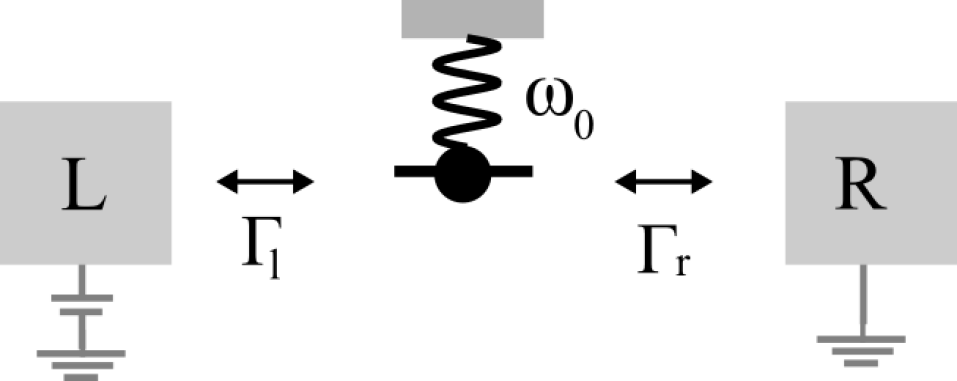
Figure 1: Sketch of a quantum dot coupled to a oscillator of frequency $\omega_{0}$. The dot’s energy level is $\varepsilon_{0}$. The quantum dot is in contacted with two normal contacts with the tunneling rates $\Gamma_{l}$ and $\Gamma_{r}$, respectively.

For the first limit case, we find several transitions from enhancement to suppression of the noise, occuring in different frequency ranges. In particular, at fixed frequency $\omega$, $S_{1}(\omega)$ shows a non-monotonic behavior as a function of $T$, with $S_{1}(\omega)>0$ at small or large transmission and negative values $S_{1}(\omega)<0$ in the intermediate range. Remarkably, for $\omega>0$, the zero order elastic noise $S_{0}(\omega)$ vanishes at $T\simeq 1$ whereas $S_{1}(\omega)$ is finite enabling the possibility to investigate the pure vibrational-induced current noise. For the second limit case, we find qualitatively similar behaviors although the relevant contribution of $S_{1}(\omega)$ is strongly localized in correspondence of characteristic lines which are associated to the resonant transport regime. Interestingly, at fixed frequency $\omega$, vibrational side bands appear as varying the dot’s level $\varepsilon_{0}$. These bands, with spacing equal to the vibrational frequency $\omega_{0}$, provide a clear signature of the charge-vibration interaction in the noise spectrum.

The paper is organized as follows. In Sec. II, we introduce the model and the Keldysh Green’s function technique. Then, in Sec. III we derive the nonsymmetrized current noise $S_{1}(\omega)$ and analyse the different kind of corrections according the technical diagrammatic approach. Section III contains the main result of the manuscript, the general formula for $S_{1}(\omega)$ of the Holstein model. In Sec. IV and V we discuss the two limit cases, the energy-independent transmission regime and the resonant transport, respectively. Sec. VI contains the final remarks.

II Model

In this section, we discuss a model of a quantum dot between conducting contacts (leads) as shown in Fig. 1.

We consider the electrons on the quantum dot occupying a spinless state with energy $\varepsilon_{0}$ and the annihilation and creation operators $\hat{d}^{\phantom{g}}$ and $\hat{d}^{\dagger}$ on the quantum dot. The occupation number reads $\hat{n}_{d}=\hat{d}^{\dagger}\hat{d}^{\phantom{g}}$. A single harmonic mode of the oscillator with frequency $\omega_{0}$ has the bosonic annihilation and creation operators $\hat{b}^{\phantom{g}}$ and $\hat{b}^{\dagger}$. We assume an interaction between the charge and the amplitude of the oscillator with coupling strength $\lambda$. The full Hamiltonian is given by

$$\hat{H}=\hat{H}_{l}+\hat{H}_{r}+\hat{H}_{t}+\varepsilon_{0}\hat{n}_{d}+\lambda\hat{n}_{d}(\hat{b}^{\dagger}+\hat{b}^{\phantom{\dagger}})+\hbar\omega_{0}\hat{b}^{\dagger}\hat{b}^{\phantom{\dagger}}\,,$$ (1)

with the last two terms describing the charge-vibration coupling and the oscillator. The Hamiltonians of the lateral leads are given by $\hat{H}_{l}=\sum_{k}\xi_{l,k}^{\phantom{\dagger}}\hat{c}^{\dagger}_{k}\hat{c}^{\phantom{\dagger}}_{k}$ and $\hat{H}_{r}=\sum_{k}\xi_{r,k}^{\phantom{\dagger}}\hat{a}^{\dagger}_{k}\hat{a}^{\phantom{\dagger}}_{k}$ with the energy $\xi_{\alpha,k}=\varepsilon_{k}-\mu_{\alpha}$ with $\alpha=(l,r)$ referring to the chemical potential. The annihilation operators are given by $\hat{c}_{k}$ for the left and $\hat{a}_{k}$ for the right lead. The tunneling Hamiltonian is $\hat{H}_{t}=\sum_{k}(t_{l}^{\phantom{\dagger}}\hat{c}^{\dagger}_{k}\hat{d}^{\phantom{\dagger}}+t_{r}^{\phantom{\dagger}}\hat{a}^{\dagger}_{k}\hat{d}^{\phantom{\dagger}}+\mathrm{H.c.})$ with the tunneling amplitudes between the leads and the dot $t_{l}$ and $t_{r}$. In the rest of our analysis we assume the wide-band approximation and consider the tunnel rates between the quantum dot with the normal contacts $\Gamma_{l}=\pi{\left|t_{l}\right|}^{2}\rho_{l}$ and $\Gamma_{r}=\pi{\left|t_{r}\right|}^{2}\rho_{r}$, respectively, with $\rho_{l}$ and $\rho_{r}$ the electron density of states at the Fermi level of the leads.

II.1 Electron Green’s functions without charge-vibration interaction $(\lambda=0)$

In this subsection we recall the exact results for the electron Green’s functions on the dot without charge-vibration interaction. These Green’s functions denoted by $G(\tau,\tau^{\prime})$ constitute the building blocks by which we can express the frequency-dependent current noise in presence of the charge-vibration interaction.

Since we are interested in the nonequilibrium properties, we defined the contour-ordered Green’s functions on the quantum dot as $G(\tau,\tau^{\prime})=-i\langle\mathcal{T}_{c}\hat{d}(\tau)\hat{d}^{\dagger}(\tau^{\prime})\rangle$ with the times $\tau$ and $\tau^{\prime}$ on the Keldysh contour and the contour-ordering operator $\mathcal{T}_{c}$ [Rammer, 2007,Cuevas and Scheer, 2010]. We then transform the contour-ordered Green’s functions to the real time and define the electron Green’s function in Keldysh space as

$$\hat{G}(t,t^{\prime})=\begin{pmatrix}{G}^{11}(t,t^{\prime})&{G}^{12}(t,t^{\prime})\\ {G}^{21}(t,t^{\prime})&{G}^{22}(t,t^{\prime})\end{pmatrix}\,.$$ (2)

with the elements of the matrix defined as ${G}^{11}(t,t^{\prime})=-i\langle{\mathcal{T}}\hat{d}(t)\hat{d}^{\dagger}(t^{\prime})\rangle$, ${G}^{22}(t,t^{\prime})=-i\langle\tilde{\mathcal{T}}\hat{d}(t)\hat{d}^{\dagger}(t^{\prime})\rangle$, ${G}^{12}(t,t^{\prime})=i\langle\hat{d}^{\dagger}(t^{\prime})\hat{d}(t)\rangle$, and ${G}^{21}(t,t^{\prime})=-i\langle\hat{d}(t)\hat{d}^{\dagger}(t^{\prime})\rangle$. In the above expression, the upper indexes $1$ or $2$ refer to the position of the times $t$ and $t^{\prime}$ on the Keldysh contour [Rammer, 2007,Cuevas and Scheer, 2010]. The real time-ordering and anti-time ordering operators are denoted by $\mathcal{T}$ and $\tilde{\mathcal{T}}$, respectively. In addition to the Green’s function in Eq. (2), we define the retarded and advanced Green’s functions as ${G}^{R}(t,t^{\prime})=-i\theta(t-t^{\prime})\langle\{\hat{d}(t),\hat{d}(t^{\prime})\}\rangle$, ${G}^{A}(t,t^{\prime})=i\theta(t^{\prime}-t)\langle\{\hat{d}(t),\hat{d}(t^{\prime})\}\rangle$, with the anti-commutator $\{\,,\,\}$. These Green’s functions are related to the ones in Eq. (2) by $G^{11}(t,t^{\prime})=G^{R,A}(t,t^{\prime})+G^{12,21}(t,t^{\prime})$ and $G^{22}(t,t^{\prime})=G^{21,12}(t,t^{\prime})-G^{R,A}(t,t^{\prime})$ (see appendix A for further details).

From the contour-ordered Green’s function, one obtains the Dyson equation

$$G(\tau,\tau^{\prime})\mathord{=}g(\tau,\tau^{\prime})+\!\!\sum_{\alpha=l,r}\!\int\!\!d\tau_{1}d\tau_{2}g(\tau,\tau_{1})\Sigma_{\alpha}(\tau_{1},\tau_{2})G(\tau_{2},\tau^{\prime})\,,$$ (3)

with $g(\tau,\tau^{\prime})$ the unperturbed dot’s Green’s functions without tunneling between the dot and the leads $\hat{H}_{t}=0$ and the self-energies of the left and right leads $\Sigma_{\alpha}(\tau,\tau^{\prime})$ [$\alpha=(l,r)$] respect to the tunneling interaction. Similarly to the Green’s functions, the self-energy appearing in Eq. (3) in Keldsyh space are defined as

$$\hat{\Sigma}_{\alpha}(t,t^{\prime})=\begin{pmatrix}{\Sigma}_{\alpha}^{11}(t,t^{\prime})&-{\Sigma}_{\alpha}^{12}(t,t^{\prime})\\ -{\Sigma}_{\alpha}^{21}(t,t^{\prime})&{\Sigma}_{\alpha}^{22}(t,t^{\prime})\end{pmatrix}\,.$$ (4)

with a minus sign on the off-diagonal elements corresponding to the different position of $t$ and $t^{\prime}$ on the Keldsyh contour. After a Fourier transformation, we obtain for the Green’s functions

$$G^{R}(\varepsilon) =[\varepsilon-\varepsilon_{0}+i(\Gamma_{l}+\Gamma_{r})]^{-1}\,$$ (5)

$$G^{12,21}(\varepsilon) =G^{R}(\varepsilon)(\Sigma_{l}^{12,21}(\varepsilon)+\Sigma_{r}^{12,21}(\varepsilon))G^{A}(\varepsilon)$$ (6)

with $G^{R}(\varepsilon)={G^{A}(\varepsilon)}^{*}$ and the self-energies of the leads

$$\Sigma_{\alpha}^{12}(\varepsilon) =2i\Gamma_{\alpha}f_{\alpha}(\varepsilon)$$ (7)

$$\Sigma_{\alpha}^{21}(\varepsilon) =-2i\Gamma_{\alpha}[1-f_{\alpha}(\varepsilon)]\,,$$ (8)

and the Fermi function $f_{\alpha}(\varepsilon)=\{1-\mathrm{exp}[\beta(\varepsilon-\mu_{\alpha})]\}^{-1}$ with the chemical potential of the left and right lead $\mu_{\alpha}$ and the inverse of the temperature $\beta$.

II.2 Phonon Green’s functions without charge-vibration interaction $(\lambda=0)$

In this subsection we recall the unperturbed phonon Green’s function for a single harmonic oscillator which will be useful to derive the frequency-dependent current noise in the presence of charge-vibration interaction. We introduce the symmetrized bosonic operator $\hat{A}(t)=\hat{b}^{\dagger}(t)+\hat{b}(t)$ and define the phonon Green’s function as $D(\tau,\tau^{\prime})=-i\langle\mathcal{T}_{c}\hat{A}(\tau)\hat{A}^{\dagger}(\tau^{\prime})\rangle$ with the time variable $\tau,\tau^{\prime}$ on the Keldysh contour. Then, we change from the contour variable $\tau$ to the real time $t$ and write the phonon Green’s function in the Keldysh space as a matrix

$$\hat{D}(t,t^{\prime})=\begin{pmatrix}D^{11}(t,t^{\prime})&D^{12}(t,t^{\prime})\\ D^{21}(t,t^{\prime})&D^{22}(t,t^{\prime})\end{pmatrix}\,,$$ (9)

with the phonon Green’s functions ${D}^{11}(t,t^{\prime})=-i\langle{\mathcal{T}}\hat{A}(t)\hat{A}^{\dagger}(t^{\prime})\rangle$, ${D}^{22}(t,t^{\prime})=-i\langle\tilde{\mathcal{T}}\hat{A}(t)\hat{A}^{\dagger}(t^{\prime})\rangle$, ${D}^{12}(t,t^{\prime})=-i\langle\hat{A}^{\dagger}(t^{\prime})\hat{A}(t)\rangle$, and ${D}^{21}(t,t^{\prime})=-i\langle\hat{A}(t)\hat{A}^{\dagger}(t^{\prime})\rangle$. The bare phonon Green’s functions read

$$D^{\mathop{}_{22}^{11}}(\varepsilon) =\sum_{s=\pm}\left[-i\pi(2n_{B}+1)\delta(\varepsilon+s\omega_{0})\pm\mathcal{P}\frac{s}{\varepsilon+s\omega_{0}}\right]$$

$$D^{\mathop{}_{21}^{12}}(\varepsilon) =-2\pi i\left[(n_{B}+1)\delta(\varepsilon\pm\omega_{0})+n_{B}\delta(\varepsilon\mp\omega_{0})\right]$$ (10)

with the Bose distribution function $n_{B}=n_{B}(\omega_{0})=[\mathrm{exp}(\beta\omega_{0})-1]^{-1}$ and the Cauchy principal value of the integral denoted by $\mathcal{P}$. For simplicity, we concentrate hereafter, in the main text, to the case of zero temperature of the vibration $n_{B}=0$.

III Nonsymmetrized current noise

In this section we summarize the perturbative expansion of the nonsymmetrized current noise $S(\omega)$ respect to the charge-vibration interaction.

We start with the definition of $S(\omega)$ and then perform a perturbative expansion in the charge-vibration coupling up to the leading order $S_{1}(\omega)\propto\lambda^{2}$. All terms of this expansion are shown in a diagrammatic representation. We obtain that the $S_{1}(\omega)$ correction can be separated into a mean-field noise and a vertex correction.

III.1 Diagrammatic approach for the noise

By using the Hamiltonian Eq. (1) we derive the current operator which is given, in the Heisenberg picture, by the expression

$$\hat{I}_{l}(t)=\frac{4ei}{\hbar}\sum_{k}t_{l}\left[\hat{c}_{k}^{\dagger}(t)\hat{d}(t)-\hat{d}^{\dagger}(t)\hat{c}_{k}(t)\right]\,.$$ (11)

We define the nonsymmetrized - frequency-dependent - current noise on the left lead as

$$S(\omega)=\int_{-\infty}^{\infty}d(t-t^{\prime})e^{-i\omega(t-t^{\prime})}\langle\hat{I}_{l}((t)\hat{I}_{l}((t^{\prime})\rangle\,.$$ (12)

The nonsymmetrized current correlator on the left lead can be defined in terms of the Keldysh Green’s functions as

$$\langle\hat{I}_{l}(t)\hat{I}_{l}(t^{\prime})\rangle =S^{21}(t,t^{\prime})\hskip 28.45274ptt>t^{\prime}$$ (13)

with the real times $t$ and $t^{\prime}$. In Eq. (13), we have introduced the Green’s functions defined on the Keldysh contour and which is expressed, generally, in terms of the times $\tau$ and $\tau^{\prime}$ on the Keldysh coutour

$$S(\tau,\tau^{\prime})=\,\langle\mathcal{T}_{c}\hat{I}_{l}(\tau)\hat{I}_{l}(\tau^{\prime})\rangle\,,$$ (14)

Then, we calculate the current-current correlation function in Eq. (14).

Without the charge-vibration coupling, the correlation function $S(\tau,\tau^{\prime})$ can be calculated exactly. However, to include the interaction to the oscillator, we use a perturbation expansion in the charge-vibration coupling $\lambda$ which allows to use Wick’s theorem and to decompose the final expression in terms of single-particle Green’s functions. As a result we obtain, that the correlator can be written in terms of the zero-order term $S_{0}(\tau,\tau^{\prime})\propto\lambda^{0}$ and the leading order correction $S_{1}(\tau,\tau^{\prime})\propto\lambda^{2}$, namely

$$S(\tau,\tau^{\prime})=S_{0}(\tau,\tau^{\prime})+S_{1}(\tau,\tau^{\prime})\,.$$ (15)

Using the diagrammatic representation, the leading order correction can be additionally decomposed into a mean-field contribution $S_{\mathrm{mf}}(\tau,\tau^{\prime})$ and a vertex correction, $S_{\mathrm{vc}}(\tau,\tau^{\prime})$,

$$S_{1}(\tau,\tau^{\prime})=S_{\mathrm{mf}}(\tau,\tau^{\prime})+S_{\mathrm{vc}}(\tau,\tau^{\prime})\,.$$ (16)

Furthermore, the mean-field correction can be divided into an elastic and an inelastic contribution with the latter associated to the absorption of a quantum energy $\omega_{0}$ by the oscillator.

$$S_{\mathrm{mf}}(\tau,\tau^{\prime})=S_{\mathrm{ec}}(\tau,\tau^{\prime})+S_{\mathrm{in}}(\tau,\tau^{\prime})\,.$$ (17)

In the following, we discuss in detail the different contributions: the zero-order term $S_{0}(\tau,\tau^{\prime})$, the two components of the mean-field correction $S_{\mathrm{ec}}(\tau,\tau^{\prime})$ and $S_{\mathrm{in}}(\tau,\tau^{\prime})$, and the vertex correction $S_{\mathrm{vc}}(\tau,\tau^{\prime})$.

Before to proceed, we introduce the notation and the symbol for the elemental block functions, defined in the previous section, and appearing in the diagrammatic representation of the noise, see Fig. 2. The contour-ordered Green’s function of the dot $G(\tau,\tau^{\prime})$ is denoted by a solid line, the self-energy on the left lead $\Sigma_{l}(\tau,\tau^{\prime})$ is denoted by a dashed line whereas the contour-ordered phonon propagator $D(\tau,\tau^{\prime})$ is depicted as a wiggled line.

Figure 2: Elements of Feynman diagrams depending on the Keldysh contour times $\tau$ and $\tau^{\prime}$. The solid and dashed line represent the Green’s function of the dot $G(\tau,\tau^{\prime})$ and the self-energy of the left lead $\Sigma_{l}(\tau,\tau^{\prime})$. The phonon propagator $D(\tau,\tau^{\prime})$ is denoted by the wiggled line.

III.2 Zero-order noise $\lambda=0$

The zero-order noise for a quantum dot has been studied and well known in the literature. Here, we simply recall the results using the diagrammatic approach.

The diagrammatric representation of the zero-order term $S_{0}(\tau,\tau^{\prime})$ is shown in Fig. 3 and corresponds to

$$S_{0}(\tau,\tau^{\prime}) =\frac{4e^{2}}{h}\int d\tau_{1}d\tau_{2}\mathrm{Re}\{G(\tau,\tau^{\prime})\Sigma_{l}(\tau^{\prime},\tau)$$

$$+G(\tau,\tau^{\prime})\Sigma_{l}(\tau^{\prime},\tau_{1})G(\tau_{1},\tau_{2})\Sigma_{l}(\tau_{2},\tau)$$

$$+G(\tau,\tau_{2})\Sigma_{l}(\tau_{1},\tau^{\prime})G(\tau^{\prime},\tau_{2})\Sigma_{l}(\tau_{2},\tau^{\prime})\}\,,$$ (18)

with $G(\tau,\tau^{\prime})$ and $\Sigma_{l}(\tau,\tau^{\prime})$ defined in Sec. II.1. The first line in Eq. (18) corresponds to the diagram in Fig. 3(a), whereas the second and third line correspond to the diagrams in Fig. 3(b) and (c), respectively. From the expression in Eq. (18) we transform from the contour time to the real time with the definition of the matrices $\hat{G}(t,t^{\prime})$ and $\hat{\Sigma}(t,t^{\prime})$ in Keldysh space given by Eq. (2) and (4). After the calculations, we obtain the frequency dependent current noise

$$S_{0} (\omega)\!=\!\frac{e^{2}}{h}\!\int\!d\varepsilon\{f_{r}(\varepsilon)(1-f_{l}(\varepsilon\!-\!\omega))T_{lr}(\varepsilon)[1-T_{lr}(\varepsilon\!-\!\omega)]$$

$$+ f_{l}(\varepsilon)(1-f_{r}(\varepsilon\!-\!\omega))T_{lr}(\varepsilon\!-\!\omega)[1-T_{lr}(\varepsilon)]$$

$$+ f_{r}(\varepsilon)(1-f_{r}(\varepsilon\!-\!\omega))T_{lr}(\varepsilon)T_{lr}(\varepsilon\!-\!\omega)+[T_{lr}(\varepsilon)T_{lr}(\varepsilon\!-\!\omega)$$

$$+ 4\Gamma_{l}^{2}|G^{R}(\varepsilon\!-\!\omega)\!-\!G^{R}(\varepsilon)|^{2}][f_{l}(\varepsilon)(1-f_{l}(\varepsilon\!-\!\omega))]\}$$ (19)

with the transmission function defined as $T_{\alpha\beta}(\varepsilon)=4\Gamma_{\alpha}\Gamma_{\beta}|G^{R}(\varepsilon)|^{2}$ and $(\alpha,\beta)=(l,r)$.

Figure 3: Diagrammatic representation of $S_{0}(\tau,\tau^{\prime})$ in Eq. (18). The solid dot is for the tunneling between the left lead and the dot. The other symbols are defined in Fig. 2.

As discussed in Ref. [Zamoum et al., 2016], one can identify to each term of Eq. (19) single processes with an absorption or emission of an energy quantum $\omega$, although such processes occur on the left lead since we calculated the current-current correlator for $\hat{I}_{l}(t)$. Indeed, in Eq. (19), all terms are proportional to products of Fermi functions such as $f_{\alpha}(\varepsilon)(1-f_{\beta}(\varepsilon-\omega))$ with $(\alpha,\beta)=(l,r)$. As an example, the first line in Eq. (19) describes a process in which an electron from the right lead is transmitted to the left lead with the emission of a photon. Similar processes can be attributed to the second term and to the third term of the sum inside the integral in Eq. (19). Whereas the first three terms are proportional to the transmission amplitude $\sim T_{lr}$, the last term also contains an additional function $\sim|G^{R}(\varepsilon-\omega)-G^{R}(\omega)|^{2}$ that represents an interference effect (see Ref. [Zamoum et al., 2016]).

III.3 Mean-field correction

The corrections proportional to $\lambda^{2}$ in the perturbation expansion are more involved. To gain some insight into the finite frequency current noise, we decompose it in several terms according the diagrammatic language.

To discuss the mean-field correction $S_{\mathrm{mf}}(\tau,\tau^{\prime})$, it is useful to introduce two building block diagrams corresponding to the rainbow (tb) and tapole (tp) diagram of the self-energy defined with respect the charge-vibration interaction. In time-domain, these objects can be written as

$$\Sigma_{\mathrm{rb}}^{\mathrm{mf}}(\tau_{1},\tau_{2})= i\lambda^{2}D(\tau_{1},\tau_{2})G(\tau_{1},\tau_{2})\,,$$ (20)

$$\Sigma_{\mathrm{tp}}^{\mathrm{mf}}(\tau_{1},\tau_{2})= -i\lambda^{2}D(\tau_{1},\tau_{2})G(\tau_{2},\tau_{2})\,,$$ (21)

and their diagrammatic representation is shown in Fig. 4(a) and (b), respectively.

With the use of the diagrams in Fig. 4, we can easily write down the contour-time Feynman diagrams contributing to the mean-field noise depicted in Fig. 5. The rectangular box in Fig. 5 represents either the rainbow or the tadpole diagram of Fig. 4. The diagrams can be divided into two kinds. The first kind of diagrams, shown in Fig. 5(a), contain a single self-energy of the left lead, two electron Green’s functions and the rectangular box. The second kind of diagrams [Fig. 5(b)] contain two self-energies of the left lead, three electron Green’s functions and the self-energies due to the electron-vibration interaction. There are four different diagrams of the second kind differing by the time labels.

Figure 4: Diagrammatic representation of Eq. (20) and (21) for the rainbow (a) and tadpole (b) diagrams. The cross represents the vertex due to the charge-vibration interaction. The other symbols are defined in Fig. 2.

Figure 5: Diagrammatic representation of $S_{\mathrm{mf}}(\tau,\tau^{\prime})$ Eq. (22). The rectangular box represents either the diagram of Fig. 4(a) or Fig. 4(b). The time arguments $\tau_{3}$ and $\tau_{4}$ are internal indexes and the diagrams can be separated into contribution without (a) and with (b) internal indexes. The solid dot is for the tunneling between the left lead and the dot. The other symbols are defined in Fig. 2.

We can write the mean-field current noise as

$$S_{\mathrm{mf}}(\tau,\tau^{\prime})=\frac{4e^{2}}{h}\sum_{\alpha=\mathrm{rb,tp}}\{\mathrm{Re}\{{\Sigma}_{l}(\tau,\tau^{\prime})A_{\mathrm{mf}}^{\alpha}(\tau^{\prime},\tau)\}$$

$$+\int d\tau_{3}d\tau_{4}\mathrm{Re}\{{G}(\tau,\tau_{3}){\Sigma}_{l}(\tau_{3},\tau^{\prime})A_{\mathrm{mf}}^{\alpha}(\tau^{\prime},\tau_{4}){\Sigma}_{l}(\tau_{4},\tau)$$

$$+A_{\mathrm{mf}}^{\alpha}(\tau,\tau_{3}){\Sigma}_{l}(\tau_{3},\tau^{\prime}){G}(\tau^{\prime},\tau_{4}){\Sigma}_{l}(\tau_{4},\tau)$$

$$-{G}(\tau,\tau^{\prime}){\Sigma}_{l}(\tau^{\prime},\tau_{3})A_{\mathrm{mf}}^{\alpha}(\tau_{3},\tau_{4}){\Sigma}_{l}(\tau_{4},\tau)$$

$$-A_{\mathrm{mf}}^{\alpha}(\tau,\tau^{\prime}){\Sigma}_{l}(\tau^{\prime},\tau_{3}){G}(\tau_{3},\tau_{4}){\Sigma}_{l}(\tau_{4},\tau)\}\}\,.$$ (22)

with the definitions

$$A^{\mathrm{rb}}_{\mathrm{mf}}(\tau,\tau^{\prime}) \mathord{=}\int d\tau_{1}d\tau_{2}\,G(\tau,\tau_{1})\Sigma^{\mathrm{rb}}_{\mathrm{mf}}(\tau_{1},\tau_{2})G(\tau_{2},\tau^{\prime})\,,$$ (23)

$$A^{\mathrm{tp}}_{\mathrm{mf}}(\tau,\tau^{\prime}) \mathord{=}\int d\tau_{1}d\tau_{2}\,G(\tau,\tau_{1})\Sigma^{\mathrm{tp}}_{\mathrm{mf}}(\tau_{1},\tau_{2})G(\tau_{1},\tau^{\prime})\,,$$ (24)

The first term in Eq. (22) corresponds to the diagrams shown in Fig. 5(a), and the following four terms to the diagrams in Fig. 5(b).

Equation (22) is the first main result of the paper and corresponds to the mean-field noise in the presence of charge-vibration interaction to the leading order in $\lambda$. For this contribution, similar to the current, we can separate the mean-field correction into an elastic term and an inelastic term, i.e. $S_{\mathrm{mf}}(\tau,\tau^{\prime})=S_{\mathrm{ec}}(\tau,\tau^{\prime})+S_{\mathrm{in}}(\tau,\tau^{\prime})$.

III.3.1 Elastic term of the mean-field correction

It turns out that the elastic term of the mean-field correction $S_{\mathrm{ec}}(\tau,\tau^{\prime})$ has the same structure of the zero-order current noise in Eq. (19) with a renormalization of the transmission functions. Indeed, it reads

$$S_{\mathrm{ec}}(\omega)=-\frac{2e^{2}}{h}\int d\varepsilon\, \left\{f_{r}(\varepsilon)(1-f_{l}(\varepsilon-\omega))[\tilde{T}_{lr}(\varepsilon)-\tilde{T}_{lr}(\varepsilon)T_{lr}(\varepsilon-\omega)-{T}_{lr}(\varepsilon)\tilde{T}_{lr}(\varepsilon-\omega)]\right.$$

$$+ f_{l}(\varepsilon)(1-f_{r}(\varepsilon-\omega))[\tilde{T}_{lr}(\varepsilon-\omega)-\tilde{T}_{lr}(\varepsilon)T_{lr}(\varepsilon-\omega)-{T}_{lr}(\varepsilon)\tilde{T}_{lr}(\varepsilon-\omega)]$$

$$+ f_{r}(\varepsilon)(1-f_{r}(\varepsilon-\omega))[\tilde{T}_{lr}(\varepsilon)T_{lr}(\varepsilon-\omega)+{T}_{lr}(\varepsilon)\tilde{T}_{lr}(\varepsilon-\omega)]$$

$$+ f_{l}(\varepsilon)(1-f_{l}(\varepsilon-\omega))[\tilde{T}_{ll}(\varepsilon)+\tilde{T}_{ll}(\varepsilon-\omega)+T_{lr}(\varepsilon)\tilde{T}_{lr}(\varepsilon-\omega)+\tilde{T}_{lr}(\varepsilon)T_{lr}(\varepsilon-\omega)$$

$$- \left.8\Gamma_{l}^{2}\mathrm{Re}[G^{A}(\varepsilon)G^{R}(\varepsilon-\omega)\Sigma^{R}(\varepsilon-\omega)G^{R}(\varepsilon-\omega)]-8\Gamma_{l}^{2}\mathrm{Re}[G^{A}(\varepsilon-\omega)G^{R}(\varepsilon)\Sigma^{R}(\varepsilon)G^{R}(\varepsilon)]]\right\}\,.$$ (25)

To formally obtain the result of Eq. (25), we have to introduce the renormalize transmission $\tilde{T}_{\alpha\beta}(\varepsilon)=T_{\alpha\beta}(\varepsilon)\mathrm{Re}[G^{R}(\varepsilon)\Sigma^{R}(\varepsilon)]$. Then, we can substitute ${T}_{\alpha\beta}(\varepsilon)$ with ${T}_{\alpha\beta}(\varepsilon)+\tilde{T}_{\alpha\beta}(\varepsilon)$ in Eq. (19) as well as substitute $G^{R}(\varepsilon)$ with $\rightarrow G^{R}(\varepsilon)+G^{R}(\varepsilon)\Sigma^{R}(\varepsilon)G^{R}(\varepsilon)$ in the last term of Eq. (19). Here, $\Sigma^{R}(\varepsilon)$ is the retarded self-energy $\Sigma^{R}(\varepsilon)$ with respect to the charge-vibration interaction (a summary of the self-energies associated to the charge-vibration interaction is given in Appendix B). Then, after these substitutions we keep only the terms proportional to $\lambda^{2}$. In this way, the elastic term to the mean-field correction corresponds to a renormalization of the transmission functions and it describes the same processes as the zero-order noise. This renormalization can be seen as a virtual exchange of absorption and emission of a phonon from the tunneling charge to the local vibration.

III.3.2 Inelastic term of the mean-field correction

The second term $S_{\mathrm{in}}(\omega)$ appearing in the mean-field corrections correspond to the inelastic processes involving the vibration, i.e. emission or absorption of a quantum energy (phonon).

As we focus on the limit of vanishing temperature for the vibration, we have only phonon emission. In other words, since the frequency-dependent current noise is related to the probability of photon emission or absorption, $S_{\mathrm{in}}(\omega)$ is associated to such processes involving not only the tunneling charge but even the emission of one vibrational quantum $\omega_{0}$. This term can be written as

$$S_{\mathrm{in}}(\omega)\!=\!\frac{ie^{2}}{2h\Gamma_{r}}\!\!\int d\varepsilon T_{lr}(\varepsilon)[f_{l}(\varepsilon)\Sigma_{21}(\varepsilon)+(1-f_{l}(\varepsilon))\Sigma_{12}(\varepsilon)]$$

$$\times\sum_{s}T_{lr}(\varepsilon+s\omega)[f_{l}(\varepsilon+s\omega)-f_{r}(\varepsilon+s\omega)]$$

$$+T_{lr}(\varepsilon)\Sigma_{12}(\varepsilon)[1-f_{l}(\varepsilon-\omega)]-T_{lr}(\varepsilon)\Sigma_{21}(\varepsilon)f_{l}(\varepsilon+\omega)\,.$$ (26)

with the self-energies $\Sigma_{12}(\varepsilon)$ and $\Sigma_{21}(\varepsilon)$ with respect to the charge-vibration interaction defined in the Appendix B. Notice that Eq. (26) is real despite the imaginary factor $i$ in front of it.

III.4 Vertex correction

The vertex correction is more difficult to analyze compared to the mean-field one. A diagrammatic representation of it is shown in Fig. 6 and its formula in terms of the times on the Keldysh contour is given in Eq. (27). In Appendix C, we illustrate the transformation of the Eq. (27) from the time defined on the Keldysh contour $\tau$ to the real time $t$.

In comparison to the mean-field results in Fig. 5, the upper and lower branch in Fig. 6(a) are connected due to the interaction with the oscillator. The diagrams in Fig. 6(a) have a similar structure as the rainbow diagrams whereas in Fig. 6(b) they a similar structure as the tadpole ones, albeit with the external times $\tau$ or $\tau^{\prime}$.

$$S_{\mathrm{vc}}(\tau,\tau^{\prime})=i\lambda^{2}\int d\tau_{1}\,d\tau_{2}\,d\tau_{3}\,d\tau_{4}\,\,\{ G(\tau,\tau_{1})G(\tau_{1},\tau_{3})\Sigma_{l}(\tau_{3},\tau^{\prime})G(\tau^{\prime},\tau_{2})G(\tau_{2},\tau_{4})\Sigma_{l}(\tau_{4},\tau)D(\tau_{1},\tau_{2})$$

$$- G(\tau,\tau_{1})G(\tau_{1},\tau^{\prime})\Sigma_{l}(\tau^{\prime},\tau_{3})G(\tau_{3},\tau_{2})G(\tau_{2},\tau_{4})\Sigma_{l}(\tau_{4},\tau)D(\tau_{1},\tau_{2})$$

$$- G(\tau,\tau_{1})G(\tau_{1},\tau_{3})\Sigma_{l}(\tau_{3},\tau)G(\tau^{\prime},\tau_{2})G(\tau_{2},\tau_{4})\Sigma_{l}(\tau_{4},\tau^{\prime})D(\tau_{1},\tau_{2})$$

$$+ G(\tau,\tau_{1})G(\tau_{1},\tau_{3})\Sigma_{l}(\tau_{3},\tau)\Sigma_{l}(\tau^{\prime},\tau_{4})G(\tau_{4},\tau_{2})G(\tau_{2},\tau^{\prime})D(\tau_{1},\tau_{2})\}$$ (27)

Figure 6: Diagrams corresponding to the vertex correction $S_{\mathrm{vc}}(\tau,\tau^{\prime})$ in Eq. (27). The solid dot is for the tunneling between the left lead and the dot. The other symbols are defined in Fig. 2.

IV Energy independent transmission regime

In principle one can evaluate numerically the different corrections to the noise for an arbitrary range of parameters. However, in order to gain some insight, we concentrate here on two limit cases that can be worked out analytically.

In the first one, we assume that the energy dependence in the Green’s functions can be neglected, e.g. we write the retarded Green’s functions as $G^{R}(\varepsilon)=G^{R}(\varepsilon_{F})$, with the energy at the Fermi level $\varepsilon_{F}$. This means in practice that the transmission is energy-independent and we note it as $T=T(\varepsilon_{F})$. This is a good approximation in two cases: (i) when the coupling to the leads is so strong that $\Gamma_{l}+\Gamma_{r}\gg\omega_{0},eV,\varepsilon_{0}$ and (ii) when the resonant level is far away from the Fermi energy, i.e. $\varepsilon_{0}\gg\Gamma_{l},\Gamma_{r},eV,\omega_{0}$ (we set $\mu_{l}=\mu_{r}=0$ in absence of applied voltage).

IV.1 Zero-order current noise $S_{0}(\omega)$

It is convenient to start with the discussion of the current noise without the interaction with the oscillator. At zero temperature, we can write the elastic current noise as

$$S_{0}(\omega)\!=\!eG\begin{cases}2\omega\quad&\omega\!<\!-eV\\ eV\!-\!\omega\!+\!T(eV\!+\!\omega)&\!-\!eV\!<\!\omega\!<\!0\\ (1\!-\!T)(eV\!-\!\omega)&0\!<\!\omega\!<\!eV\\ 0&\omega\!>\!eV\end{cases}$$ (28)

with the conductance $G=2e^{2}T/h$. $S_{0}(\omega)$ shows a linear piecewise dependence on the frequency $\omega$ and $eV$.

Figure 7 shows $S_{0}(\omega)$ as a function of the transmission $T$ and the frequency $\omega$. When $\omega>eV$, the noise is zero since a photon due to a single electron tunneling event here examined - can only be emitted with a maximal energy given by the applied bias voltage $\omega=eV$. When $\omega<-eV$, the current noise scales as $G\omega$ such that in Fig. 7 the current noise seems to be independent of the transmission. In the region $0<\omega<eV$, the current noise linearly decreases with increasing transmission and vanishes at $T=1$. A similar behavior appears when $-eV<\omega<0$ in which the current noise decreases from $eV-\omega$ to $2eV$ by increasing the transmission. Finally, for perfect transmission $T=1$, the noise vanished at positive frequency.

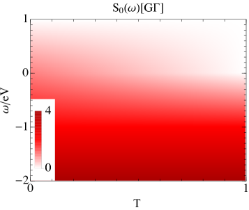
Figure 7: Zero-order current noise $S_{0}(\omega)$ as a function of transmission $T$ and noise frequency $\omega$.

IV.2 Correction to the noise $S_{1}(\omega)$

In this section we analyze the correction $S_{1}(\omega)$ to the finite-frequency current noise due to the charge-vibration interaction in the limit of energy independent transmission of the quantum dot.

The charge-vibration interaction leads to a suppression or an enhancement of the current noise: as shown in Fig. 8: depending on the transmission $T$ and the frequency $\omega$, $S_{1}(\omega)$ can be positive or negative. Such a complex behavior is caused by the interplay of the mean-field corrections and the vertex correction. We note that the corrections to the current noise is scaled with $\lambda^{2}$ and the total noise is positive for all parameter range.

Although the elastic term $S_{\mathrm{ec}}(\omega)$ and the inelastic term $S_{\mathrm{in}}(\omega)$, of the mean field correction and the vertex correction $S_{\mathrm{vc}}(\omega)$ can be further simplified under the assumption of energy-independent transmissions, here we discuss the full expression $S_{1}(\omega)$ for energy-independent transmission. The detailed expressions for the individual terms are given in Appendix D. Generally, $S_{1}(\omega)$ has a piecewise linear dependence of the current noise on the frequency $\omega$ controlled by the frequency of the oscillator $\omega_{0}$ and the voltage $eV$. When $\omega>eV$, the noise correction $S_{1}(\omega)$ vanishes in similar way as $S_{0}(\omega)$, as previously discussed. We distinguish two regimes depending on the frequency of the oscillator and the voltage. The first regime is given by $\omega_{0}<eV$ in which the voltage is sufficiently large to excite the oscillator. In the second one $\omega_{0}<eV$, the voltage is smaller than the frequency of the oscillator such that an additional absorption of a photon by the electron is needed to excite the oscillator.

For $eV>\omega_{0}$, the correction to the noise is given by

$$S^{eV>\omega_{0}}_{1}(\omega)\!=\!\frac{\lambda^{2}e^{2}T^{2}}{2\Gamma^{2}}\!\!\begin{cases}\left(4T\!-\!3\right)\omega\!+\!(2T\!-\!1)\omega_{0}&\omega\!<\!-eV-\omega_{0}\\ \left(3T\!-\!\frac{5}{2}\right)\omega\!+\!(T\!-\!\frac{1}{2})\omega_{0}-\left(T-\frac{1}{2}\right)eV&-eV-\omega_{0}\!<\!\omega\!<\!-eV\\ \left(4T^{2}-2T-\frac{3}{2}\right)\omega+(T-\frac{1}{2})\omega_{0}+\left(4T^{2}-6T+\frac{3}{2}\right)eV&-eV\!<\!\omega\!<\!\mathrm{min}(-\omega_{0},-eV+\omega_{0})\\ \left(2T^{2}-\frac{3}{2}\right)\omega-\left(2T^{2}-3T+\frac{1}{2}\right)\omega_{0}+\left(4T^{2}-6T+\frac{3}{2}\right)eV\\ \hskip 36.98866pt-T(eV(1-2T)+(3-4T)\omega+\omega_{0})\theta(eV-2\omega_{0})&\mathrm{min}(\!-\!\omega_{0},\omega_{0}\!-\!eV)\!<\!\omega\!<\!\mathrm{max}(\!-\!\omega_{0},\omega_{0}\!-\!eV)\\ \left(4T^{2}\!-\!T\!-\!\frac{3}{2}\right)\omega\!-\!(4T^{2}\!-\!4T\!+\!\frac{1}{2})\omega_{0}\!+\!\left(6T^{2}\!-\!7T+\frac{3}{2}\right)eV&\mathrm{max}(-\omega_{0},\omega_{0}-eV)\!<\!\omega\!<\!0\\ \left(5T\!-\!4T^{2}\!-\!\frac{3}{2}\right)\omega\!-\!(4T^{2}\!-\!4T\!+\!\frac{1}{2})\omega_{0}\!+\!\left(6T^{2}\!-\!7T\!+\!\frac{3}{2}\right)eV&0\!<\!\omega\!<\!\mathrm{min}(\omega_{0},eV-\omega_{0})\\ \left(\!-\!2T^{2}\!+\!3T\!-\!1\right)\omega\!+\!2T(1\!-\!T)\omega_{0}\!+\!(1\!-\!T)(1\!-\!4T)eV\\ \hskip 22.76228pt+\!\frac{1}{2}(eV(1\!-\!2T)^{2}\!-\!(1\!-\!8T(1\!-\!T))\omega\!-\!\omega_{0})\theta(eV\!-\!2\omega_{0})&\mathrm{min}(\omega_{0},eV-\omega_{0})\!<\!\omega\!<\!\mathrm{max}(\omega_{0},eV-\omega_{0})\\ \left(-4T^{2}+5T-1\right)\omega+(1-T)(1-4T)eV&\mathrm{max}(\omega_{0},eV-\omega_{0})\!<\!\omega\!<\!eV\\ 0&\omega\!>\!eV\end{cases}$$ (29)

For $\omega<eV$, the noise shows a linear dependence as a function of $\omega$ which can be divided into nine frequency intervals. The behavior of the noise Eq. (29) is illustrated in Fig. 8(a) as a function of the transmission $T$ and frequency $\omega$ for $\omega_{0}=0.25eV$. The separation of the correction to the noise in intervals appears as a kink in the frequency-dependence, i. e. at $\omega=0,\pm\omega_{0},-eV+\omega_{0},-eV$ and $\omega_{0}=-eV-\omega_{0}$. For the other intervals of Eq. (29), the change in slope is too small to reveal the kinks in Fig. 8(a). The transition from the positive to the negative correction to the emission noise in the interval $eV-\omega_{0}<\omega<eV$ appears at $T=0.25$ and is independent from the oscillator frequency $\omega_{0}$ as long as $\omega_{0}<eV$, see Eq. (29). In the interval $-\omega_{0}<\omega<eV-\omega_{0}$, the correction to the noise is positive for small transmission, becomes negative by increasing the transmission and is again positive when $T\rightarrow 1$. Such a double transition as has been obtained for the shot noise ($\omega=0$) in Ref. [Haupt et al., 2009] and measured in Ref. [Kumar et al., 2012]. Here we demonstrate that such a double transition also appears at finite frequencies. Finally, when $\omega<-\omega_{0}$, the correction to the noise has a single transition in which it switches from positive to negative values as increasing the transmission $T$.

Interesting features appear in $S_{1}(\omega)$ for the emission noise ($\omega>0$) at perfect transmission $T=1$. In this case, the vertex correction vanishes at positive frequencies. The noise $S_{1}(\omega)$ is given only by the mean-field corrections and vanishes when $\omega>eV-\omega_{0}$ due to the cancellation of the elastic correction and the inelastic one, as can be seen from Eqs. (75) and (76) in the Appendix. However, $S_{1}(\omega)$ is finite and positive when $0<\omega<eV-\omega_{0}$. Here, as recalled in the previous section, the zero-order noise $S_{0}(\omega)$ vanishes for positive frequencies at $T=1$, e.g. it scales linearly to zero as $1-T$. Hence, a finite emission noise for perfect transmission (or close to it $T\rightarrow 1$) can be an intrinsic signature of the charge-vibration interaction of the quantum transport through the tunnel junction.

We now turn to the discussion of the correction to the noise for $eV<\omega_{0}$. In this case the oscillator cannot be inelastically be excited. The corrections to the noise can be divided into eight intervals

$$S^{eV<\omega_{0}}_{1}(\omega)=\frac{\lambda^{2}e^{2}}{2h\Gamma^{2}}T^{2}\begin{cases}(4T-3)\omega+(2T-1)\omega_{0}&\omega<-eV-\omega_{0}\\ (3T-\frac{5}{2})\omega+(T-\frac{1}{2})\omega_{0}+(\frac{1}{2}-T)eV&-eV-\omega_{0}<\omega<-\omega_{0}\\ (3T-\frac{5}{2})\omega+(T-\frac{1}{2})\omega_{0}-eV(T-\frac{1}{2})&-\omega_{0}<\omega<-eV\\ (2T^{2}-\frac{3}{2})\omega+(T-\frac{1}{2})\omega+(2T^{2}-4T+\frac{3}{2})eV&-eV<\omega<eV-\omega_{0}\\ -(1-T)(1+2T)\omega+eV(1-T)(1-2T)&eV-\omega_{0}<\omega<0\\ (-2T^{2}+3T-1)\omega+(T-1)(2T-1)eV&0<\omega<eV\\ 0&\omega>eV\,.\end{cases}$$ (30)

Figure 11(b) shows the correction to the noise at $\omega_{0}=1.25eV$. In this case the correction to the noise is positive at small transmission and changes sign once time by increasing the transmission. Interestingly, the sign change in the emission noise $(\omega>0)$ appears at $T=0.5$ independent of $\omega_{0}$ as long as $\omega_{0}>eV$.

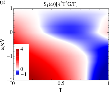
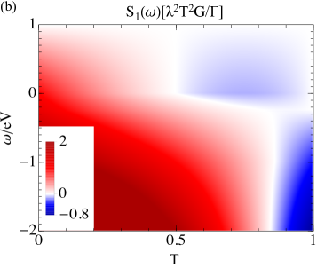
Figure 8: Correction to the noise $S_{1}(\omega)$ as a function of transmission $T$ and frequency $\omega$. In (a) $\omega_{0}=0.25eV$ and in (b) $\omega_{0}=1.25eV$. In (a) the correction to the noise shows a double transition in the frequency range $-\omega_{0}<\omega<eV-\omega_{0}$ from positive to negative value. At $T=1$, $S_{1}(\omega)$ is finite and positive in the frequency range $0<\omega<eV-\omega_{0}$, in contrast to the zero-order noise $S_{0}(\omega)=0$ in Fig. 7.

V Resonant transmission regime

In this section, we focus on the regime in which the electrons tunnel through the resonant level at $\varepsilon_{0}$. This regime is characterized by a tunneling coupling much smaller then the voltage and the frequency of the oscillator with tunneling rates $\Gamma_{l},\Gamma_{r}\ll eV,\omega_{0}$. In this case we have to take the energy-dependence of the Green’s functions appearing the zero-order noise [Eq. (19)], the elastic term [Eq. (25)] and the inelastic term [Eq. (26)] of the mean-field correction, and the vertex correction [Eq. (27)] into account. We report here the numerical results of these expressions. Similar to the previous section, we first study the zero-order noise $S_{0}(\omega)$ and then we discuss the correction $S_{1}(\omega)$.

V.1 Zero-order current noise $S_{0}(\omega)$

Figure 9 shows $S_{0}(\omega)$ as a function of the gate voltage $\varepsilon_{0}$ and the frequency $\omega$. The voltage is applied on the left lead $\mu_{l}=eV$ and $\mu_{r}=0$. Since we discuss the resonant regime, we fix a small coupling to the leads with $\Gamma_{l}=\Gamma_{r}=0.01eV$.

First, consider the case of the emission noise $(\omega>0)$. Since the voltage is applied on the left lead, an electron with energy $\varepsilon=\mu_{l}$ can tunnel from the left chemical potential to the quantum dot at $\varepsilon_{0}$ and thereby emit a photon with energy $\omega=eV-\varepsilon_{0}$. An example of this process is shown in the inset of Fig. 10(a) for $\varepsilon_{0}=0$. Then, when then gate voltage in increased, e.g. $\varepsilon_{0}=eV/2$, the maximal energy for the electron to emit a photon reduces to $eV/2$. In other words, in the resonant transport regime here discussed, the effective, maximal energy of the photon emitted is given by $eV-\varepsilon_{0}>0$. Eventually, when the energy level of the quantum dot is tuned outside the voltage bias region, $\varepsilon_{0}>eV$ or $\varepsilon_{0}<0$, an electron cannot tunnel through the resonant level and the noise vanishes.

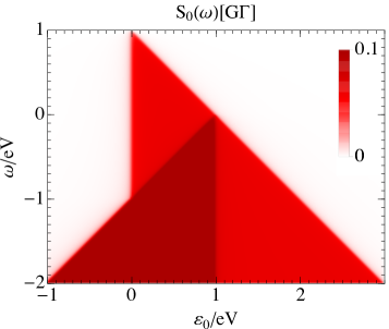
Figure 9: Current noise $S_{0}(\omega)$ as a function of the dot’s energy level $\varepsilon_{0}$ and noise frequency $\omega$ at zero temperature. The coupling to the leads is symmetric $\Gamma_{l}=\Gamma_{r}=\Gamma$ with $\Gamma=0.01eV$.

We now consider the absorption noise at negative frequencies ($\omega<0$). Similar to the emission noise, the effective, minimum amount of absorbed energy by a photon is given by $|\varepsilon_{0}-eV|$ otherwise the electron from the lead lead can not tunnel into the dot’s level. Thus the current (absorption) noise vanishes again for $\varepsilon_{0}>eV$.

To illustrate the general behavior in this frequency range, we can assume $\varepsilon_{0}=0$ for simplicity. When $|\omega|<eV$, a photon is absorbed by the electrons from the quantum dot’s level and then tunnel only to the right lead since $\omega<eV$. An example of such an absorption process in shown in the right inset of Fig. 10(b). This absorption process with the tunneling to the right lead appears for all frequencies in the range $|\omega|<eV$. However, when the frequency is larger than the voltage $|\omega|>eV$, an electron from the quantum dot’s level at $\varepsilon_{0}=0$ can, after the absorption of a photon, tunnel to the right or the left lead, Fig. 10(c) leading to an increase of the current noise. Similar discussion is valid at finite values of $\varepsilon_{0}$, albeit that the electron can also tunnel from the leads to the dot, and it explains the step-like increase of the current noise corresponding to the dark red region in Fig. 9.

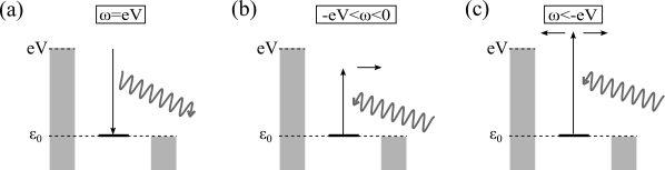
Figure 10: Schematic of processes corresponding to the emission (a) and absorption (b,c) of a photon for the resonant transport regime at $\varepsilon_{0}=0$. These processes explain the behavior of the elastic noise in Fig. 9. In (a), a photon with the maximal frequency $\omega=eV$ is emitted by the contact. In (b) an electron is excited by absorbing a photon with energy smaller than the voltage. After the excitation, the electron can only tunnel to the right lead. In (c), the photon has an energy larger than the voltage such that the excited electron can tunnel to the left and right lead.

V.2 Correction to the noise $S_{1}(\omega)$

In this section we discuss the correction to the noise $S_{1}(\omega)$ in the resonant transport regime.

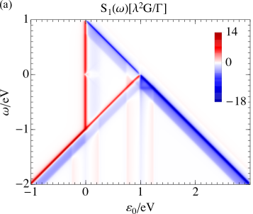
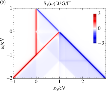
Figure 11: Correction to the noise $S_{1}(\omega)$ as a function of the frequency $\omega$ and the quantum dot’s energy level $\varepsilon_{0}$. The coupling to the leads is symmetric $\Gamma_{l}=\Gamma_{r}=\Gamma=0.01eV$. The oscillator’s frequency is set to (a) $\omega_{0}=0.25eV$ and (b) $\omega_{0}=1.25eV$.

Figure 11 shows the correction $S_{1}(\omega)$ to the noise as a function of the energy level $\varepsilon_{0}$ of the quantum dot and the frequency $\omega$ for the oscillator’s frequency $\omega_{0}=0.25eV$ and $\omega_{0}=1.25eV$. The pattern of $S_{1}(\omega)$ reflects the behavior of the zero-order current noise typical of the resonant transport regime, as shown in Fig. 9. However, the noise correction in Fig. 11 vanishes in extended regions of the diagram as a function of $\omega$ and $\varepsilon_{0}$. As we show in Appendix E in Fig. 12, the vanishing of $S_{1}(\omega)$ is related to the exact cancellation of the inelastic noise and the mean-field elastic term of the mean-field corrections.

To discuss the characteristic features of the oscillator in the noise $S_{1}(\omega)$, we start with a oscillator frequency $\omega_{0}=0.25eV$ as a representative case for $\omega_{0}<eV$ [Fig. 11(a)].

Again, we consider first the case $\varepsilon_{0}=0$. In the range $|\omega|<eV$, the correction to the noise is positive and drops at $\omega=-eV$ to a negative value in the range $-eV<\omega<-eV-\omega_{0}$. When $\omega<-eV-\omega_{0}$ the correction slightly increases but remains negative. A qualitative argument to explain such sharp transition from a positive to a negative correction at $\omega=-eV$ is as follows. Since the oscillator is at zero temperature, it can only absorb a vibrational energy quantum $\omega_{0}$. In the range $-eV<\omega<-eV-\omega_{0}$, an electron is excited form the quantum dot’s level at $\varepsilon_{0}=0$ to an energy above the left chemical potential and, in absence of charge-vibration interaction, it can tunnel to the left or right lead. However, due to the interaction, the excited electron can emit a phonon at frequency $\omega_{0}$ losing some energy. After the emission, the electron has hence an energy below the left chemical potential and hence can only tunnel to the right lead. On the basis of the discussion for the zero-order noise in Sec. V.1, this explains the reduction of the noise and the reason why the correction results to be negative in the interval $-eV<\omega<-eV-\omega_{0}$ at $\varepsilon_{0}=0$. Similar arguments hold at finite values of $\varepsilon_{0}$, where the noise is suppressed within the frequency range $-eV+\varepsilon_{0}<\omega<-eV+\varepsilon_{0}-\omega_{0}$ for $\varepsilon_{0}<eV$. Furthermore, a region of negative correction also appears below the line $\omega=eV-\varepsilon_{0}$ for $\varepsilon_{0}>0$ in the frequency range $eV-\omega_{0}-\varepsilon_{0}<\omega<eV-\varepsilon_{0}$ for $0<\varepsilon_{0}<eV-\omega_{0}$ (emission noise) and $\varepsilon_{0}>eV$ (absorption noise).

Another interesting feature appears when $\varepsilon_{0}$ is tuned close the left $\varepsilon_{0}\sim eV$ or to the right $\varepsilon_{0}\sim 0$ chemical potential. In the region delimited by $\omega<-eV+\varepsilon_{0}$ and $\omega<eV-\varepsilon_{0}$, at given frequency $\omega$, vibrational side bands appear in form of peaks (negative or positive) at $\varepsilon_{0}=\pm\omega_{0}$ and $\varepsilon_{0}=eV\pm\omega_{0}$. These two lateral peaks appear when the inelastic emission of a phonon is in resonance with the lateral chemical potentials. In this case, for instance, an electron inelastically emits a phonon by tunneling either from the level to the right chemical potential ($\varepsilon_{0}=+\omega_{0}$) or from the right chemical potential to the quantum dot ($\varepsilon_{0}=-\omega_{0}$). In both cases the energy to excite the oscillator solely comes from the applied voltage explaining the independence of the two side peaks as a function of frequency. A similar arguments holds when the gate voltage is tuned such that the level position is close to the left chemical potential, i.e $\varepsilon_{0}=eV$.

It is also interesting to note that in the range $eV<\varepsilon_{0}<eV+\omega_{0}$, a resonant (negative) peak appears exactly at $\omega=-\omega_{0}$. In this case we argue that the photon energy absorbed by the whole system, quantum dot and oscillator, is resonant with the local vibration.

As an example of the case $\omega_{0}>eV$, Figure 11(b) shows the correction to the noise for $\omega_{0}=1.25eV$. Here, $S_{1}(\omega)$ has similar features as the Fig. 11(a) with the negative correction band below the diagonal lines having now a larger width of $\omega_{0}=1.25eV$. Additionally, the lateral side peaks are less visible compared to the previous case.

VI Conclusion

We study the frequency-dependent current noise in the Holstein model for a quantum dot between two normal-conducting leads, in the perturbative limit which covers several realistic experimental cases, such as single molecule junctions or suspended carbon nanotube quantum dots. We focused on two limiting cases: the regime of energy-independent transmissions, in which we derived analytical expressions for the current noise, and the regime of the resonant transport. Our analysis and predictions, based on analytic formulas for the Holstein model, constitute a reference for future studies of the frequency-dependent noise in tunnel junction with local charge-vibration interaction in more complex transport situations (many conducting channels, multi-level dots, etc.). Finally, for the case of energy-independent transmission, we found that the noise induced by the interaction of the dot’s charge with the vibration represents the only contribution to the noise for high transmission of the junction $T\simeq 1$. This calls for an experimental investigation of this noise using on-chip detectors, thus providing direct information on the vibrational states of the junction.

Appendix A Keldysh Green’s functions

In this appendix, we recall the definitions and some relations of the Green’s functions which are used in the main text. We refer to the books of Refs. [Rammer, 2007,Cuevas and Scheer, 2010] for a detailed introduction. The Green’s functions are defined as (we omit the spatial dependence)

$${G}(t,t^{\prime}) ={G}^{11}(t,t^{\prime})=-i\langle{\mathcal{T}}\psi(t)\psi^{\dagger}(t^{\prime})\rangle\,,$$ (31)

$$\tilde{G}(t,t^{\prime}) ={G}^{22}(t,t^{\prime})=-i\langle\tilde{\mathcal{T}}\psi(t)\psi^{\dagger}(t^{\prime})\rangle\,,$$ (32)

$${G}^{<}(t,t^{\prime}) ={G}^{12}(t,t^{\prime})=i\langle\psi^{\dagger}(t^{\prime}),\psi(t)\rangle\,,$$ (33)

$${G}^{>}(t,t^{\prime}) ={G}^{21}(t,t^{\prime})=-i\langle\psi(t)\psi^{\dagger}(t^{\prime})\rangle\,,$$ (34)

$${G}^{R}(t,t^{\prime}) =-i\theta(t-t^{\prime})\langle\{\psi(t),\psi^{\dagger}(t^{\prime})\}\rangle\,,$$ (35)

$${G}^{A}(t,t^{\prime}) =i\theta(t^{\prime}-t)\langle\{\psi(t),\psi^{\dagger}(t^{\prime})\}\rangle\,,$$ (36)

$${G}^{K}(t,t^{\prime}) =-i\langle[\psi(t),\psi^{\dagger}(t^{\prime})]\rangle\,.\$$ (37)

with the commutator denoted with $[\,,\,]$ and the field operator $\psi(t)$ in the Heisenberg picture. In the case of bosonic field operators, the commutator is replaced $[\,,\,]$ by the anticommutator $\{\,,\,\}$ and a minus sign must be added in the lesser Green’s function.

The electron Green’s functions satisfy the following relations

$$G^{R}(t,t^{\prime})-G^{A}(t,t^{\prime}) =G^{>}(t,t^{\prime})-G^{<}(t,t^{\prime})$$ (38)

$$G^{K}(t,t^{\prime}) =G^{11}(t,t^{\prime})+{G}^{22}(t,t^{\prime})$$

$$=G^{<}(t,t^{\prime})+{G}^{>}(t,t^{\prime})$$ (39)

$$G^{R}(t,t^{\prime}) =G^{11}(t,t^{\prime})-G^{<}(t,t^{\prime})$$

$$=G^{>}(t,t^{\prime})-{G}^{22}(t,t^{\prime})$$ (40)

$$G^{A}(t,t^{\prime}) =G^{<}(t,t^{\prime})-{G}^{22}(t,t^{\prime})$$

$$=G^{11}(t,t^{\prime})-{G}^{>}(t,t^{\prime})$$ (41)

$$G^{11}(t,t^{\prime}) =G^{R}(t,t^{\prime})+G^{<}(t,t^{\prime})$$

$$=G^{A}(t,t^{\prime})+G^{>}(t,t^{\prime})$$ (42)

$$G^{22}(t,t^{\prime}) =G^{<}(t,t^{\prime})-G^{A}(t,t^{\prime})$$

$$=G^{>}(t,t^{\prime})-G^{R}(t,t^{\prime})$$ (43)

and

$$G^{<}(t,t^{\prime}) =(G^{K}(t,t^{\prime})-G^{R}(t,t^{\prime})+G^{A}(t,t^{\prime}))/2$$ (44)

$$G^{>}(t,t^{\prime}) =(G^{K}(t,t^{\prime})+G^{R}(t,t^{\prime})-G^{A}(t,t^{\prime}))/2$$ (45)

Further, the hermitian-conjugate of the electron Green’s functions satisfy the relations

$${G^{R}(t,t^{\prime})}^{*} =G^{A}(t^{\prime},t)$$ (46)

$${G^{<}(t,t^{\prime})}^{*} =-G^{<}(t^{\prime},t)$$ (47)

$${G^{>}(t,t^{\prime})}^{*} =-G^{>}(t^{\prime},t)$$ (48)

$${G^{11}(t,t^{\prime})}^{*} =-G^{22}(t^{\prime},t)$$ (49)

$${G^{22}(t,t^{\prime})}^{*} =-G^{11}(t^{\prime},t)$$ (50)

The same relations are satisfied if the electron field operators are replaced with bosonic field operators.

Appendix B The electron self-energy with respect to the charge-vibration interaction

We define the self-energies $\Sigma^{11}$ as the following matrices

$$\hat{\Sigma}(\varepsilon)=\begin{pmatrix}\Sigma^{11}(\varepsilon)&-\Sigma^{12}(\varepsilon)\\ -\Sigma^{21}(\varepsilon)&\Sigma^{22}(\varepsilon)\end{pmatrix}$$ (51)

with a minus sign in front of $\Sigma^{12}(\varepsilon)$ and $\Sigma^{21}(\varepsilon)$ due to the different position of the time arguments on the Keldysh contour. The leading order of the self-energy with respect to the charge-vibration coupling are proportional to $\lambda^{2}$ and are given by

$$\Sigma^{11}(\varepsilon) \!\!=\!\!\lambda^{2}\sum_{s}\left[\frac{1}{2}[1+n_{B}(\omega_{0})]G^{11}(\varepsilon+s\omega_{0})\right.$$ (52)

$$-\left.\frac{i}{2\pi}\mathcal{P}\int d\varepsilon^{\prime}\frac{s}{\varepsilon^{\prime}+s\omega_{0}}G^{11}(\varepsilon-\varepsilon^{\prime})\right]$$ (53)

$$\Sigma^{12}(\varepsilon) \!\!=\!\!\lambda^{2}n_{B}(\omega_{0})[G^{12}(\varepsilon-\omega_{0})\!\!+\!\!(1+n_{B}(\omega_{0}))G^{12}(\varepsilon+\omega_{0})]$$ (54)

$$\Sigma^{21}(\varepsilon) \!\!=\!\!\lambda^{2}n_{B}(\omega_{0})[G^{21}(\varepsilon+\omega_{0})\!\!+\!\!(1+n_{B}(\omega_{0}))G^{21}(\varepsilon-\omega_{0})]$$ (55)

$$\Sigma^{22}(\varepsilon) \!\!=\!\!\lambda^{2}\sum_{s}\left[\frac{1}{2}[1+n_{B}(\omega_{0})]G^{22}(\varepsilon+s\omega_{0})\right.$$ (56)

$$+\left.\frac{i}{2\pi}\mathcal{P}\int d\varepsilon^{\prime}\frac{s}{\varepsilon^{\prime}+s\omega_{0}}G^{22}(\varepsilon-\varepsilon^{\prime})\right]$$ (57)

$$\Sigma^{R}(\varepsilon) \!\!=\!\!\Sigma^{11}(\varepsilon)-\Sigma^{12}(\varepsilon)$$ (58)

$$\Sigma^{A}(\varepsilon) \!\!=\!\!\Sigma^{12}(\varepsilon)-\Sigma^{22}(\varepsilon)$$ (59)

with the frequency $\omega_{0}$ of the oscillator, the Bose-distribution function $n_{B}(\omega)$, and the Cauchy principal value $\mathcal{P}$ of the integral. In the previous formulas, the electronic Green’s functions $G$ are the dot’s function in absence of interaction with the vibration.

Appendix C Real-time vertex current noise

In this appendix we transform the vertex correction from the Keldysh contour time integration to the real time integration.

To this end, we first cast the vertex correction in terms of rainbow-like and tadpole-like diagrams. The vertex correction in Eq. (27) can be written as

$$S_{\mathrm{vc}}(\tau,\tau^{\prime})=$$

$$G(\tau,\tau_{1})\Sigma_{\mathrm{rb}}^{\nu}(\tau_{1},\tau_{2})G(\tau_{2},\tau_{3})\Sigma_{l}(\tau_{3},\tau)$$

$$+ \left.G(\tau,\tau_{1})\Sigma_{\mathrm{tp}}^{\nu}(\tau_{2},\tau_{2})G(\tau_{1},\tau_{3})\Sigma_{l}(\tau_{3},\tau)\right\}\,.$$ (60)

Here, we defined the rainbow-like and tadpole-like self-energies $\Sigma_{\mathrm{rb}}^{\nu}(\tau_{1},\tau_{2})$ and $\Sigma_{\mathrm{tb}}^{\nu}(\tau_{1},\tau_{2})$ with $\nu=(\Romannum{1},\Romannum{2})$ respectively. We remark that the energies $\Sigma_{\mathrm{rb}}^{\nu}(\tau_{1},\tau_{2})$ and $\Sigma_{\mathrm{tb}}^{\nu}(\tau_{1},\tau_{2})$ implicitly depend on the external time $\tau^{\prime}$ [see Eqn. (63)-(66)].

The difference between the self-energies labeled with $\Romannum{1}$ and $\Romannum{2}$ comes from the dependence of the Green’s function and self-energies on the external time $\tau^{\prime}$. The rainbow-like and tadpole-like diagrams are

$$\Sigma_{\mathrm{rb}}^{\nu}(\tau_{1},\tau_{2}) =i\lambda^{2}C_{\mathrm{rb}}^{\nu}(\tau_{1},\tau_{2})D(\tau_{1},\tau_{2})$$ (61)

$$\Sigma_{\mathrm{tp}}^{\nu}(\tau_{1},\tau_{2}) =-i\lambda^{2}C_{\mathrm{tp}}^{\nu}(\tau_{2})D(\tau_{1},\tau_{2})$$ (62)

with the functions $C_{\mathrm{rb}}^{\nu}$ and $C_{\mathrm{rb}}^{\nu}$ given by

$$C_{\mathrm{rb}}^{\Romannum{1}}(\tau_{1},\tau_{2}) =\int d\tau_{4}G(\tau_{1},\tau_{4})\Sigma_{l}(\tau_{4},\tau^{\prime})G(\tau^{\prime},\tau_{2})\,,$$ (63)

$$C_{\mathrm{rb}}^{\Romannum{2}}(\tau_{1},\tau_{2}) =\int d\tau_{4}G(\tau_{1},\tau^{\prime})\Sigma_{l}(\tau^{\prime},\tau_{4})G(t_{4},\tau_{2})\,,$$ (64)

and

$$C_{\mathrm{tp}}^{\Romannum{1}}(\tau_{2}) =\int d\tau_{4}G(\tau_{2},\tau_{4})\Sigma_{l}(\tau_{4},\tau^{\prime})G(\tau^{\prime},\tau_{2})\,,$$ (65)

$$C_{\mathrm{tp}}^{\Romannum{2}}(\tau_{2}) =\int d\tau_{4}G(\tau_{2},\tau^{\prime})\Sigma_{l}(\tau^{\prime},\tau_{4})G(\tau_{4},\tau_{2})\,.$$ (66)

The functions $C_{\mathrm{tp}}^{\alpha}(\tau_{2})$ depend only on the time $\tau_{2}$ but not on $\tau_{1}$.

Second, we transform the vertex correction from the time on the Keldysh contour to the real time and perform a Fourier transformation. When transforming Eq. (60) from the contour to the real time, we introduce the matrix Green’s functions defined in Eq. (2). To give an example, the following term

$$A(\tau,\tau^{\prime})=\int d\tau_{1}G(\tau,\tau_{1})\Sigma_{l}(\tau_{1},\tau^{\prime})$$ (67)

transform as

$$\hat{A}(t,t^{\prime})=\int dt_{1}\hat{G}(t,t_{1})\hat{\tau}_{K}\hat{\Sigma}_{l}(t_{1},t^{\prime})$$ (68)

where we have the Pauli matrix $\hat{\tau}_{K}$ with $1$ and $-1$ for diagonal elements which takes into account the position of the contour time $\tau_{1}$ on the Keldysh contour, see Ref.[Rammer, 2007]. Finally, the crucial step to calculate the current noise vertex corrections is to transform the rainbow- and tadpole-like diagrams in Eq. (61) and (62) in the real time representation and perform a Fourier transformation. The rainbow-like diagrams can be written as

$$\hat{\Sigma}_{\mathrm{rb}}^{\nu}(\varepsilon) =i\lambda^{2}\int\frac{d\varepsilon^{\prime}}{2\pi}\begin{pmatrix}C_{\mathrm{rb}}^{\nu,11}(\varepsilon-\varepsilon^{\prime})D^{11}(\varepsilon)&-C_{\mathrm{rb}}^{\nu,12}(\varepsilon-\varepsilon^{\prime})D^{12}(\varepsilon)\\ -C_{\mathrm{rb}}^{\nu,21}(\varepsilon-\varepsilon^{\prime})D^{21}(\varepsilon)&C_{\mathrm{rb}}^{\nu,22}(\varepsilon-\varepsilon^{\prime})D^{22}(\varepsilon)\end{pmatrix}\,,$$ (69)

with the functions

$$\hat{C}_{\mathrm{rb}}^{\Romannum{1}}(\varepsilon) =\begin{pmatrix}G^{11}(\varepsilon-\omega)&G^{12}(\varepsilon-\omega)\\ G^{21}(\varepsilon-\omega)&G^{22}(\varepsilon-\omega)\end{pmatrix}\check{\tau}_{K}\begin{pmatrix}0&\Sigma_{l}^{12}(\varepsilon-\omega)\\ 0&\Sigma_{l}^{22}(\varepsilon-\omega)\end{pmatrix}\begin{pmatrix}0&0\\ G^{21}(\varepsilon)&G^{22}(\varepsilon)\end{pmatrix}$$ (70)

$$\hat{C}_{\mathrm{rb}}^{\Romannum{2}}(\varepsilon) =\begin{pmatrix}0&G^{12}(\varepsilon-\omega)\\ 0&G^{22}(\varepsilon-\omega)\end{pmatrix}\begin{pmatrix}0&0\\ \Sigma_{l}^{21}(\varepsilon)&\Sigma_{l}^{22}(\varepsilon)\end{pmatrix}\check{\tau}_{K}\begin{pmatrix}G^{11}(\varepsilon)&G^{12}(\varepsilon)\\ G^{21}(\varepsilon)&G^{22}(\varepsilon)\end{pmatrix}\,.$$ (71)

Similary, the tadpole-like diagrams are given by

$$\hat{\Sigma}_{\mathrm{tp}}^{\nu} =-i\lambda^{2}\begin{pmatrix}D^{R}(-\omega)&0\\ 0&-D^{A}(-\omega)\end{pmatrix}\int\frac{d\varepsilon^{\prime}}{2\pi}\hat{C}^{\nu,12}_{\mathrm{tp}}(\varepsilon^{\prime})$$ (72)

with

$$\hat{C}_{\mathrm{tp}}^{\Romannum{1}}(\varepsilon) =\begin{pmatrix}G^{11}(\varepsilon-\omega)&G^{12}(\varepsilon-\omega)\\ G^{21}(\varepsilon-\omega)&G^{22}(\varepsilon-\omega)\end{pmatrix}\check{\tau}_{K}\begin{pmatrix}0&\Sigma_{l}^{12}(\varepsilon-\omega)\\ 0&\Sigma_{l}^{22}(\varepsilon-\omega)\end{pmatrix}\begin{pmatrix}0&0\\ G^{21}(\varepsilon)&G^{22}(\varepsilon)\end{pmatrix}$$ (73)

$$\hat{C}_{\mathrm{tp}}^{\Romannum{2}}(\varepsilon) =\begin{pmatrix}0&G^{12}(\varepsilon-\omega)\\ 0&G^{22}(\varepsilon-\omega)\end{pmatrix}\begin{pmatrix}0&0\\ \Sigma_{l}^{21}(\varepsilon)&\Sigma_{l}^{22}(\varepsilon)\end{pmatrix}\check{\tau}_{K}\begin{pmatrix}G^{11}(\varepsilon)&G^{12}(\varepsilon)\\ G^{21}(\varepsilon)&G^{22}(\varepsilon)\end{pmatrix}\,.$$ (74)

Appendix D Individual corrections $S_{\mathrm{mf}}=S_{\mathrm{ec}}+S_{\mathrm{in}}$ and $S_{\mathrm{vc}}$ for the energy-independent transmission regime.

As discussed in the manuscript, the corrections to the noise can be divided into a mean-field elastic correction and vertex correction. In this appendix, we report analytic formulas for the individual contributions to the $S_{1}(\omega)$ in the case of energy-independent transmissions. When $eV>\omega_{0}$, these corrections are given by

$$S^{eV>\omega_{0}}_{\mathrm{in}}(\omega) =\frac{\lambda^{2}e^{2}T^{2}}{4h\Gamma^{2}}\begin{cases}-4(\omega+\omega_{0})&\omega<-eV-\omega_{0}\\ eV-3\omega-3\omega_{0}&-eV-\omega_{0}<\omega<-eV\\ eV(1-T)-(3+T)\omega-3\omega_{0}&-eV<\omega<\mathrm{min}(-\omega_{0},-eV+\omega_{0})\\ eV(1-T)-\omega-(1-T)\omega_{0}\\ \hskip 14.22636pt-\theta(eV-2\omega_{0})(eVT+2((1+T)\omega+\omega_{0}))&\mathrm{min}(-\omega_{0},\omega_{0}-eV)<\omega<\mathrm{max}(-\omega_{0},\omega_{0}-eV)\\ eV(1-2T)-(1+T)\omega-(1-2T)\omega_{0}&\mathrm{max}(-\omega_{0},\omega_{0}-eV)<\omega<0\\ eV(1-2T)-(1-T)\omega-(1-2T)\omega_{0}&0<\omega<\mathrm{min}(\omega_{0},eV-\omega_{0})\\ (-eV+\omega_{0})T\\ +\theta(eV-2\omega_{0})(eV(1-T)-(1-2T)\omega-\omega_{0})&\mathrm{min}(\omega_{0},eV-\omega_{0})<\omega<\mathrm{max}(\omega_{0},eV-\omega_{0})\\ (-eV+\omega)T&\mathrm{max}(\omega_{0},eV-\omega_{0})<\omega<eV\\ 0&\omega>eV\end{cases}$$ (75)

$$S^{eV>\omega_{0}}_{\mathrm{ec}}(\omega)\! =\!\frac{\lambda^{2}e^{2}T^{2}}{4h\Gamma^{2}}\begin{cases}-4(1\!-\!2T)\omega\!+\!4T\omega_{0}&\omega\!<\!-\!eV\!-\!\omega_{0}\\ -eVT+(-4+7T)\omega+3T\omega_{0}&-eV-\omega_{0}<\omega<-eV\\ eV(2-8T+6T^{2})-2\omega+3T(2T\omega+\omega_{0})&-eV<\omega<\mathrm{min}(-\omega_{0},-eV+\omega_{0})\\ eV(2\!-\!8T\!+\!6T^{2})\!-\!(2\!+\!T(1\!-\!4T))\omega\!+\!2(1\!-\!T)T\omega_{0}\\ +T(2eVT+\omega+4T\omega+\omega_{0})\theta(eV-2\omega_{0})&\mathrm{min}(-\omega_{0},\omega_{0}-eV)<\omega<\mathrm{max}(-\omega_{0},\omega_{0}-eV)\\ 2eV(1\!-\!2T)^{2}\!-\!(1\!+\!2T)(2\!-\!3T)\omega\!+\!2(1\!-\!2T)T\omega_{0}&\mathrm{max}(-\omega_{0},\omega_{0}-eV)<\omega<0\\ (-1+2T)(eV(-2+4T)+(2-3T)\omega-2T\omega_{0})&0<\omega<\mathrm{min}(\omega_{0},eV-\omega_{0})\\ (-1+2T)(eV(-2+3T)+2\omega-T(2\omega+\omega_{0})\\ +T(eV-2\omega)\theta(eV-2\omega_{0}))&\mathrm{min}(\omega_{0},eV-\omega_{0})<\omega<\mathrm{max}(\omega_{0},eV-\omega_{0})\\ (2+T(-7+6T))(eV-\omega)&\mathrm{max}(\omega_{0},eV-\omega_{0})<\omega<eV\\ 0&\omega>eV\end{cases}$$ (76)

$$S^{eV>\omega_{0}}_{\mathrm{vc}}(\omega) =\frac{\lambda^{2}e^{2}T^{2}}{4h\Gamma^{2}}\begin{cases}2(\omega+\omega_{0})&\omega<-eV-\omega_{0}\\ 2(\omega+\omega_{0})-T(eV+\omega+\omega_{0})&-eV-\omega_{0}<\omega<-eV\\ T(-3+2T)(eV+\omega)-T\omega_{0}+2(\omega+\omega_{0})&-eV<\omega<\mathrm{min}(-\omega_{0},-eV+\omega_{0})\\ T(eV(-3+2T)+\omega+3\omega_{0}-2T\omega_{0})+\theta(eV-2\omega_{0})\\ (T(eV(-1+2T)-5\omega+4T\omega-3\omega_{0})+2(\omega+\omega_{0}))&\mathrm{min}(-\omega_{0},\omega_{0}-eV)<\omega<\mathrm{max}(-\omega_{0},\omega_{0}-eV)\\ 4T(eV(-1+T)+1/2T(\omega-2\omega_{0})+\omega_{0})&\mathrm{max}(-\omega_{0},\omega_{0}-eV)<\omega<0\\ 2(-1+T)T(2eV-\omega-2\omega_{0})&0<\omega<\mathrm{min}(\omega_{0},eV-\omega_{0})\\ 2(-1+T)T(eV-\omega_{0}+(eV-2\omega)\theta(eV-2\omega_{0}))&\mathrm{min}(\omega_{0},eV-\omega_{0})<\omega<\mathrm{max}(\omega_{0},eV-\omega_{0})\\ 2(-1+T)T(eV-\omega)&\mathrm{max}(\omega_{0},eV-\omega_{0})<\omega<eV\\ 0&\omega>eV\end{cases}$$ (77)

It is interesting to note, that for perfect transmission $T=1$, the emission noise $S^{eV>\omega_{0}}_{\mathrm{vc}}(\omega)$ vanishes due to the factor $1-T$. As discussed Sec. IV the emission noise vanishes too for $\omega>eV-\omega_{0}$ at perfect transmission. From the Eqs. (75) and (77) this can be explained by the exact cancellation of the two mean-field contributions, the inelastic and the elastic term, in the interval $\mathrm{max}(\omega_{0},eV-\omega_{0})<\omega<eV$.

When the voltage is smaller than the frequency of the oscillator, $eV<\omega_{0}$ the contributions to the correction to the noise are

$$S^{eV<\omega_{0}}_{\mathrm{in}}(\omega) =\frac{\lambda^{2}e^{2}}{4h\Gamma^{2}}T^{2}\begin{cases}-4(\omega+\omega_{0})&\omega<-eV-\omega_{0}\\ eV-3(\omega+\omega_{0})&-eV-\omega_{0}<\omega<-\omega_{0}\\ eV-\omega-\omega_{0}&-\omega_{0}<\omega<-eV\\ eV-\omega-\omega_{0}&-eV<\omega<eV-\omega_{0}\\ 0&eV-\omega_{0}<\omega\end{cases}$$ (78)

$$S^{eV<\omega_{0}}_{\mathrm{ec}}(\omega) =\frac{\lambda^{2}e^{2}}{4h\Gamma^{2}}T^{2}\begin{cases}(-4+8T)\omega+4T\omega_{0}&\omega<-eV-\omega_{0}\\ -eVT+(-4+7T)\omega+3T\omega_{0}&-eV-\omega_{0}<\omega<-\omega_{0}\\ -4\omega+T(-eV+5\omega+\omega_{0})&-\omega_{0}<\omega<-eV\\ eV(2+T(-7+4T))+(-2+T(-1+4T))\omega+T\omega_{0}&-eV<\omega<eV-\omega_{0}\\ 2(-1+T)(eV(-1+2T)+\omega+2T\omega)&eV-\omega_{0}<\omega\\ 2(-1+T)(-1+2T)(eV-\omega)&0<\omega<eV\\ 0&\omega>eV\end{cases}$$ (79)

$$S^{eV<\omega_{0}}_{\mathrm{vc}}(\omega) =\frac{\lambda^{2}e^{2}}{4h\Gamma^{2}}T^{2}\begin{cases}2(\omega+\omega_{0})&\omega<-eV-\omega_{0}\\ 2(\omega+\omega_{0})-T(eV+\omega+\omega_{0})&-eV-\omega_{0}<\omega<-\omega_{0}\\ T(-eV+\omega+\omega_{0})&-\omega_{0}<\omega<-eV\\ T(-eV+\omega+\omega_{0})&-eV<\omega<eV-\omega_{0}\\ 0&eV-\omega_{0}<\omega\end{cases}$$ (80)

Appendix E Individual corrections $S_{\mathrm{mf}}=S_{\mathrm{ec}}+S_{\mathrm{in}}$ and $S_{\mathrm{vc}}$ for the resonant transport.

In this appendix we rerpot the different contributions of the correction to the noise $S_{1}(\omega)$ shown in Fig. 11 for the case of resonant transport regime.

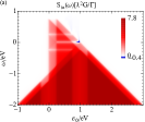
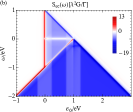
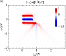
Figure 12: Contributions to $S_{1}(\omega)$ as a function as a function of the frequency $\omega$ and the quantum dot’s energy level $\varepsilon_{0}$. The coupling to the leads is symmetric $\Gamma_{l}=\Gamma_{r}=\Gamma=0.01eV$ and the oscillator’s frequency is set to $\omega_{0}=0.25eV$.

The inelastic term of the mean-field correction to the noise is reported in Fig. 12(a). whereas the elastic term of the mean-field correction in Fig. 12(b). Remarkably, in extended regions of the phase diagram $\omega$ and $\varepsilon_{0}$, the inelastic term and the elastic term perfectly cancel leading to a finite correction only close to the characteristic lines associated to the resonant transport. These lines correspond to the stepd of the zero-order noise $S_{0}(\omega)$, see Fig. 9. Similarly, the vertex correction has a relevant and sharp contribution close to these lines and in correspondence of the vibrational sideband at $\omega=0,\pm\omega_{0}$ in the range $0<\varepsilon_{0}<eV$.

References

- Blanter and Büttiker (2000) Y. M. Blanter and M. Büttiker, Phys. Rep. 336, 1 (2000).
- (2) T. Martin, Noise in Mesoscopic Physics, Les Houches Session LXXXI, edited by H. Bouchiat et al. (Elsevier 2005).
- Landauer (1998) R. Landauer, Nature 392, 658 (1998).
- Callen and Welton (1951) H. B. Callen and T. A. Welton, Phys. Rev. 83, 34 (1951).
- Nazarov and Blanter (2009) Y. V. Nazarov and Y. M. Blanter, Quantum Transport , Introduction to Nanoscience (Cambridge University Press, Cambridge, England, 2009).
- (6) Y. V. Nazarov, Quantum Noise in Mesoscopic Physics.
- Karimi et al. (2016) M. A. Karimi, S. G. Bahoosh, M. Herz, R. Hayakawa, F. Pauly, and E. Scheer, Nano Lett. 16, 1803 (2016).
- Djukic and van Ruitenbeek (2006) D. Djukic and J. M. van Ruitenbeek, Nano Lett. 6, 789 (2006).
- Tal et al. (2008) O. Tal, M. Krieger, B. Leerink, and J. M. van Ruitenbeek, Phys. Rev. Lett. 100, 196804 (2008).
- Kiguchi et al. (2008) M. Kiguchi, O. Tal, S. Wohlthat, F. Pauly, M. Krieger, D. Djukic, J. C. Cuevas, and J. M. van Ruitenbeek, Phys. Rev. Lett. 101, 046801 (2008).
- Jain (1989) J. K. Jain, Phys. Rev. Lett. 63, 199 (1989).
- Kane and Fisher (1994) C. L. Kane and M. P. A. Fisher, Phys. Rev. Lett. 72, 724 (1994).
- Saminadayar et al. (1997) L. Saminadayar, D. C. Glattli, Y. Jin, and B. Etienne, Phys. Rev. Lett. 79, 2526 (1997).
- Lesovik and Loosen (1997) G. B. Lesovik and R. Loosen, Pis’ma Zh. Eksp. Teor. Fiz. 65, 295 (1997).
- Gavish et al. (2000) U. Gavish, Y. Levinson, and Y. Imry, Phys. Rev. B 62, R10637 (2000).
- Aguado and Kouwenhoven (2000) R. Aguado and L. P. Kouwenhoven, Phys. Rev. Lett. 84, 1986 (2000).
- Glazman and Shekhter (1988) L. I. Glazman and R. I. Shekhter, Sov. Phys. JETP 67, 163 (1988).
- Wingreen et al. (1989) N. S. Wingreen, K. W. Jacobsen, and J. W. Wilkins, Phys. Rev. B 40, 11834 (1989).
- König et al. (1996) J. König, H. Schoeller, and G. Schön, Phys. Rev. Lett. 76, 1715 (1996).
- Boese and Schoeller (2001) D. Boese and H. Schoeller, Europhys. Lett.) 54, 668 (2001).
- Lundin and McKenzie (2002) U. Lundin and R. H. McKenzie, Phys. Rev. B 66, 075303 (2002).
- Kuo and Chang (2002) D. M.-T. Kuo and Y. C. Chang, Phys. Rev. B 66, 085311 (2002).
- McCarthy et al. (2003) K. D. McCarthy, N. Prokof’ev, and M. T. Tuominen, Phys. Rev. B 67, 245415 (2003).
- Braig and Flensberg (2003) S. Braig and K. Flensberg, Phys. Rev. B 68, 205324 (2003).
- Flensberg (2003) K. Flensberg, Phys. Rev. B 68, 205323 (2003).
- Galperin et al. (2004) M. Galperin, M. A. Ratner, and A. Nitzan, The Journal of Chemical Physics 121, 11965 (2004).
- Mitra et al. (2004) A. Mitra, I. Aleiner, and A. J. Millis, Phys. Rev. B 69, 245302 (2004).
- Wegewijs and Nowack (2005) M. R. Wegewijs and K. C. Nowack, New J. Phys. 7, 239 (2005).
- Kaat and Flensberg (2005) G. A. Kaat and K. Flensberg, Phys. Rev. B 71, 155408 (2005).
- Koch and von Oppen (2005a) J. Koch and F. von Oppen, Phys. Rev. Lett. 94, 206804 (2005a).
- Koch and von Oppen (2005b) J. Koch and F. von Oppen, Phys. Rev. B 72, 113308 (2005b).
- Zazunov et al. (2006) A. Zazunov, D. Feinberg, and T. Martin, Phys. Rev. B 73, 115405 (2006).
- Koch et al. (2006a) J. Koch, M. Semmelhack, F. von Oppen, and A. Nitzan, Phys. Rev. B 73, 155306 (2006a).
- Koch et al. (2006b) J. Koch, F. von Oppen, and A. V. Andreev, Phys. Rev. B 74, 205438 (2006b).
- Hwang et al. (2007) M.-J. Hwang, M.-S. Choi, and R. López, Phys. Rev. B 76, 165312 (2007).
- Lüffe et al. (2008) M. C. Lüffe, J. Koch, and F. von Oppen, Phys. Rev. B 77, 125306 (2008).
- Tahir and MacKinnon (2008) M. Tahir and A. MacKinnon, Phys. Rev. B 77, 224305 (2008).
- Schmidt and Komnik (2009) T. L. Schmidt and A. Komnik, Phys. Rev. B 80, 041307 (2009).
- Avriller and Levy Yeyati (2009) R. Avriller and A. Levy Yeyati, Phys. Rev. B 80, 041309 (2009).
- Entin-Wohlman et al. (2009) O. Entin-Wohlman, Y. Imry, and A. Aharony, Phys. Rev. B 80, 035417 (2009).
- Haupt et al. (2009) F. Haupt, T. Novotný, and W. Belzig, Phys. Rev. Lett. 103, 136601 (2009).
- Haupt et al. (2010) F. Haupt, T. Novotný, and W. Belzig, Phys. Rev. B 82, 165441 (2010).
- Schultz (2010) M. G. Schultz, Phys. Rev. B 82, 155408 (2010).
- Urban et al. (2010) D. F. Urban, R. Avriller, and A. Levy Yeyati, Phys. Rev. B 82, 121414 (2010).
- Cavaliere et al. (2010) F. Cavaliere, E. Mariani, R. Leturcq, C. Stampfer, and M. Sassetti, Phys. Rev. B 81, 201303 (2010).
- Yar et al. (2011) A. Yar, A. Donarini, S. Koller, and M. Grifoni, Phys. Rev. B 84, 115432 (2011).
- Piovano et al. (2011) G. Piovano, F. Cavaliere, E. Paladino, and M. Sassetti, Phys. Rev. B 83, 245311 (2011).
- Novotný et al. (2011) T. Novotný, F. Haupt, and W. Belzig, Phys. Rev. B 84, 113107 (2011).
- Fang et al. (2011) T.-F. Fang, Q.-f. Sun, and H.-G. Luo, Phys. Rev. B 84, 155417 (2011).
- Li et al. (2012) Z.-Z. Li, S.-H. Ouyang, C.-H. Lam, and J. Q. You, Phys. Rev. B 85, 235420 (2012).
- Skorobagatko (2012) G. A. Skorobagatko, Phys. Rev. B 85, 075310 (2012).
- Rastelli et al. (2012) G. Rastelli, M. Houzet, L. Glazman, and F. Pistolesi, Comptes Rendus Physique 13, 410 (2012).
- Santamore et al. (2013) D. H. Santamore, N. Lambert, and F. Nori, Phys. Rev. B 87, 075422 (2013).
- Härtle et al. (2013) R. Härtle, M. Butzin, and M. Thoss, Phys. Rev. B 87, 085422 (2013).
- Knap et al. (2013) M. Knap, E. Arrigoni, and W. von der Linden, Phys. Rev. B 88, 054301 (2013).
- Walter et al. (2013) S. Walter, B. Trauzettel, and T. L. Schmidt, Phys. Rev. B 88, 195425 (2013).
- Agarwalla et al. (2015) B. K. Agarwalla, J.-H. Jiang, and D. Segal, Phys. Rev. B 92, 245418 (2015).
- Schinabeck et al. (2016) C. Schinabeck, A. Erpenbeck, R. Härtle, and M. Thoss, Phys. Rev. B 94, 201407 (2016).
- Sowa et al. (2017) J. K. Sowa, J. A. Mol, G. A. D. Briggs, and E. M. Gauger, Phys. Rev. B 95, 085423 (2017).
- Ryndyk et al. (2006) D. A. Ryndyk, M. Hartung, and G. Cuniberti, Phys. Rev. B 73, 045420 (2006).
- Zazunov and Martin (2007) A. Zazunov and T. Martin, Phys. Rev. B 76, 033417 (2007).
- Egger and Gogolin (2008) R. Egger and A. O. Gogolin, Phys. Rev. B 77, 113405 (2008).
- Dash et al. (2010) L. K. Dash, H. Ness, and R. W. Godby, The Journal of Chemical Physics 132, 104113 (2010).
- Rastelli et al. (2010) G. Rastelli, M. Houzet, and F. Pistolesi, Europhys. Lett. 89, 57003 (2010).
- Dash et al. (2011) L. K. Dash, H. Ness, and R. W. Godby, Phys. Rev. B 84, 085433 (2011).
- Seoane Souto et al. (2014) R. Seoane Souto, A. Levy Yeyati, A. Martín-Rodero, and R. C. Monreal, Phys. Rev. B 89, 085412 (2014).
- Chen et al. (2016) H.-T. Chen, G. Cohen, A. J. Millis, and D. R. Reichman, Phys. Rev. B 93, 174309 (2016).
- Mera et al. (2015) H. Mera, T. G. Pedersen, and B. K. Nikolić, Phys. Rev. Lett. 115, 143001 (2015).
- Pavlyukh (2017) Y. Pavlyukh, Sci Rep 7, 601 (2017).
- Mühlbacher and Rabani (2008) L. Mühlbacher and E. Rabani, Phys. Rev. Lett. 100, 176403 (2008).
- Hützen et al. (2012) R. Hützen, S. Weiss, M. Thorwart, and R. Egger, Phys. Rev. B 85, 121408 (2012).
- Eidelstein et al. (2013) E. Eidelstein, D. Goberman, and A. Schiller, Phys. Rev. B 87, 075319 (2013).
- Jovchev and Anders (2013) A. Jovchev and F. B. Anders, Phys. Rev. B 87, 195112 (2013).
- Seoane Souto et al. (2015) R. Seoane Souto, R. Avriller, R. C. Monreal, A. Martín-Rodero, and A. Levy Yeyati, Phys. Rev. B 92, 125435 (2015).
- Engel and Loss (2004) H.-A. Engel and D. Loss, Phys. Rev. Lett. 93, 136602 (2004).
- Rothstein et al. (2009) E. A. Rothstein, O. Entin-Wohlman, and A. Aharony, Phys. Rev. B 79, 075307 (2009).
- Ding and Dong (2013) G.-H. Ding and B. Dong, Phys. Rev. B 87, 235303 (2013).
- Moca et al. (2014) C. P. Moca, P. Simon, C.-H. Chung, and G. Zaránd, Phys. Rev. B 89, 155138 (2014).
- Zamoum et al. (2016) R. Zamoum, M. Lavagna, and A. Crépieux, Phys. Rev. B 93, 235449 (2016).
- Crépieux et al. (2017) A. Crépieux, S. Sahoo, T. Q. Duong, R. Zamoum, and M. Lavagna, arXiv:1708.01187 (2017).
- Orth et al. (2012) C. P. Orth, D. F. Urban, and A. Komnik, Phys. Rev. B 86, 125324 (2012).
- Jin et al. (2015) J. Jin, S. Wang, X. Zheng, and Y. Yan, J. Chem. Phys. 142, 234108 (2015).
- Braun et al. (2006) M. Braun, J. König, and J. Martinek, Phys. Rev. B 74, 075328 (2006).
- Cottet et al. (2008) A. Cottet, B. Doucot, and W. Belzig, Phys. Rev. Lett. 101, 257001 (2008).
- Droste et al. (2015) S. Droste, J. Splettstoesser, and M. Governale, Phys. Rev. B 91, 125401 (2015).
- Lefloch et al. (2003) F. Lefloch, C. Hoffmann, M. Sanquer, and D. Quirion, Phys. Rev. Lett. 90, 067002 (2003).
- Reydellet et al. (2003) L. H. Reydellet, P. Roche, D. C. Glattli, B. Etienne, and Y. Jin, Phys. Rev. Lett. 90, 176803 (2003).
- Gabelli and Reulet (2009) J. Gabelli and B. Reulet, J. Stat. Mech. 01, 01049 (2009).
- Ubbelohde et al. (2011) N. Ubbelohde, C. Fricke, C. Flindt, F. Hohls, and R. J. Haug, Nat. Commun. 3, 612 (2011).
- Basset et al. (2012) J. Basset, A. Y. Kasumov, C. P. Moca, G. Zaránd, P. Simon, H. Bouchiat, and R. Deblock, Phys. Rev. Lett. 108, 046802 (2012).
- Basset et al. (2010) J. Basset, H. Bouchiat, and R. Deblock, Phys. Rev. Lett. 105, 166801 (2010).
- Onac et al. (2006) E. Onac, F. Balestro, B. Trauzettel, C. F. J. Lodewijk, and L. P. Kouwenhoven, Phys. Rev. Lett. 96, 026803 (2006).
- Ferrier et al. (2017) M. Ferrier, T. Arakawa, T. Hata, R. Fujiwara, R. Delagrange, R. Deblock, Y. Teratani, R. Sakano, A. Oguri, and K. Kobayashi, Phys. Rev. Lett. 118, 196803 (2017).
- Kumar et al. (2012) M. Kumar, R. Avriller, A. Levy Yeyati, and J. M. van Ruitenbeek, Phys. Rev. Lett. 108, 146602 (2012).
- Rammer (2007) J. Rammer, Quantum Field Theory of Nonequilibrium States, 1st ed. (Cambridge University Press, New York, 2007).
- Cuevas and Scheer (2010) J. C. Cuevas and E. Scheer, Molecular Electronics: An introduction to Theory and Experiment, 1st ed. (World Scientific, Singapore, 2010).