Bounding Errors Due to Switching Delays in Incrementally Stable Switched Systems (Extended Version)

Abstract

Time delays pose an important challenge in networked control systems, which are now ubiquitous. Focusing on switched systems, we introduce a framework that provides an upper bound for errors caused by switching delays. Our framework is based on approximate bisimulation, a notion that has been previously utilized mainly for symbolic (discrete) abstraction of state spaces. Notable in our framework is that, in deriving an approximate bisimulation and thus an error bound, we use a simple incremental stability assumption (namely $\delta$-GUAS) that does not itself refer to time delays. That this is the same assumption used for state-space discretization enables a two-step workflow for control synthesis for switched systems, in which a single Lyapunov-type stability witness serves for two different purposes of state discretization and coping with time delays. We demonstrate the proposed framework with a boost DC-DC converter, a common example of switched systems.

1 Introduction

Time Delays

Networked control—digital control of physical systems via computer networks—represents an important aspect in various emerging system design paradigms, such as cyber-physical systems and the Internet of Things. Consequently, identifying and addressing challenges inherent in networked control has become a crucial part of the design of reliable real-world systems.

The biggest challenge in networked control, besides limited communication capacities and packet losses, is time delay. Physical separation of plants from controllers leads to inevitable communication delays dictated by the speed of light. Worse, the rise of cloud control is making both physical and logical distances between components even longer and more unpredictable. Precise estimation of communication delays is often hard, let alone reducing them.

These trends in control engineering call for a uniform framework for robustness against potential time delays. In this paper, inspired by the hybrid nature of systems that is intrinsic to networked control, we turn to approximate bisimulation for coping with delays.

Approximate Bisimulation

An approximate bisimulation is a binary relation between states of two systems, that witnesses the proximity of the systems’ behaviors. The notion was first introduced in Girard and Pappas (2007) as a quantitative relaxation of bisimulation, a well-established coinductive equivalence notion between discrete transition systems by Park (1981). Approximate bisimulation has been actively studied ever since: a notable theoretical result is its connection to incremental stability in Pola et al. (2008); on the application side, it has been widely used in (discretized) symbolic abstraction of continuous systems.

In this paper we focus on switched systems, and use an approximate bisimulation for error bounds between: a system $\Sigma_{\tau,\delta_{0}}$ with bounded time delays; and the corresponding system $\Sigma_{\tau}$ without delays. The choice of switched systems as our subject is justified by the envisaged applications in networked control. In a switched system, a plant has finitely many operation modes; and mode changes are dictated by a switching signal that is sent from a controller over a computer network. This simple modeling encompasses various real-world networked control systems. Moreover, it turns out that our focus on switched systems greatly aids the analysis of effects of time delays.

Approximate Bisimulation for Switching Delays

Our contributions in technical terms are as follows. Our system model $\Sigma_{\tau,\delta_{0}}$ is a (potentially nonlinear) switched system where switching signals are nearly periodic with a period $\tau$; the system exhibits potential switching delays within a prescribed bound $\delta_{0}$. Our interest is in the difference between the behaviors of $\Sigma_{\tau,\delta_{0}}$ and those of the delay-free simplification $\Sigma_{\tau}$. We turn the two systems into (discrete-time) transition systems $T(\Sigma_{\tau,\delta_{0}})$ and $T(\Sigma_{\tau})$; between them we establish an approximate bisimulation that witnesses proximity of their behaviors. The approximate bisimulation is derived from an incremental stability assumption of the dynamics of the system $\Sigma_{\tau,\delta_{0}}$ (namely $\delta$-GUAS). More specifically, we present a construction that turns a Lyapunov-type witness for $\delta$-GUAS into an approximate bisimulation.

Our workflow just described resembles those in existing works about the use of approximate bisimulation. That is,

• starting from an incrementally stable system $T$, one devises an abstraction $T^{\text{abst}}$ of the system,

• establishing an approximate bisimulation between $T$ and $T^{\text{abst}}$ out of a Lyapunov-like witness of stability.

• Then the outcome of analysis of $T^{\text{abst}}$ (verification, control synthesis, etc.) can be carried over to the original system $T$, modulo the error bounded by the approximate bisimulation.

One novelty of the current work is that, unlike most of the existing works that aim at a symbolic (discrete) abstraction of a state space, our abstraction $T^{\text{abst}}=\Sigma_{\tau}$ is a temporally idealized system without switching delays.

Lyapunov-like witnesses of stability, for the purpose of bounding errors caused by time delays, have already been used in the works by Pola et al. (2010b, a). Compared to these existing works, the current work is distinguished in that we rely only on a standard and relatively simple notion of stability, that does not refer to time delays per se. Indeed, what we rely on is $\delta$-GUAS—the same stability notion used for state-space discretization in many existing works. The abundance of analyses of $\delta$-GUAS in the literature (e.g. Pola et al. (2008); Girard et al. (2010); Girard (2010)) suggests that our use of it is an advantage when it comes to application to various concrete systems. See §8 for further discussions on related work.

Figure 1: A two-step control synthesis workflow for switched systems with delays. We separate two concerns: time delays and state-space discretization. The same stability assumption on $\Sigma_{\tau}$ can be used once for all, for establishing both $\sim_{\varepsilon_{1}}$ and $\sim_{\varepsilon_{2}}$.

Two-Step Control Synthesis for Switched Systems with Delays

Even better, our reliance on the standard notion of $\delta$-GUAS enables the following two-step synthesis workflow, where we combine the current results and those in Girard et al. (2010). See Fig. 1. Our current results are used to derive the first error bound $\varepsilon_{1}$ between (the transition system $T(\Sigma_{\tau,\delta_{0}})$ derived from) the original system $\Sigma_{\tau,\delta_{0}}$, and (the transition system $T(\Sigma_{\tau})$ derived from) the delay-free abstraction $\Sigma_{\tau}$. The latter system $\Sigma_{\tau}$ is a delay-free periodic switched system, to which we can apply the state-space discretization technique in Girard et al. (2010). We thus construct a discretized symbolic model $T_{\tau}^{\text{symb}}$ and establish the second approximate bisimulation $\sim_{\varepsilon_{2}}$ in Fig. 1. The fact that our construction relies on the same stability assumptions used in Girard et al. (2010) means the following: for establishing both of the approximate bisimulations $\sim_{\varepsilon_{1}}$ and $\sim_{\varepsilon_{2}}$, we can reuse the same ingredient (namely a $\delta$-GUAS Lyapunov function), instead of finding two different Lyapunov functions.

Once we obtain a symbolic model, we can apply to it various discrete techniques, such as automata-theoretic synthesis (as in Vardi (1995)), supervisory control of discrete event systems (as in Ramadge and Wonham (1987)), algorithmic game theory (as in Arnold et al. (2003)), etc. This is the horizontal arrow at the bottom of Fig. 1. The resulting controller (i.e.  a switching signal, in the current setting) is then guaranteed, by the two approximate bisimulations, to work well with $\Sigma_{\tau}$ (with precision $\varepsilon_{2}$) and with $\Sigma_{\tau,\delta_{0}}$ (with precision $\varepsilon_{1}+\varepsilon_{2}$).

This way we ultimately derive a switching signal for the original system $\Sigma_{\tau,\delta_{0}}$ whose precision $\varepsilon_{1}+\varepsilon_{2}$ is guaranteed. The workflow in Fig. 1 takes two steps that separate concerns (namely time delays and discretization of state spaces). While this two-step approach can potentially lead to loss of generality (especially in comparison with Pola et al. (2010a), see §8), it seems to help coping with the problem’s complexity. We demonstrate our workflow in §7, where we successfully derive a controller for a boost DC-DC converter example with additional switching delays.

Contributions

Overall, our contributions are summarized as follows. We present a construction of an approximate bisimulation between a nearly-periodic switched systems and its (exactly) periodic approximation. This allows us to bound the difference between trajectories due to switching delays. Thanks to our focus on switched systems we can use a common stability assumption (namely $\delta$-GUAS) as the ingredient of the construction; this allows us to combine the current results with the existing results on symbolic abstraction and control synthesis, leading to a two-step control synthesis workflow (Fig. 1) where the same stability analysis derives two approximate bisimulations.

We defer proofs and another example (besides the boost DC-DC converter in §7) to the appendices.

2 Switched Systems

The set of nonnegative real numbers is denoted by $\mathbb{R}^{+}$. We let $\|\_\|$ denote the usual Euclidean norm on $\mathbb{R}^{n}$.

Definition 2.1 (switched system)

A switched system is a quadruple $\Sigma=(\mathbb{R}^{n},P,{\mathcal{P}},F)$ that consists of:

• a state space $\mathbb{R}^{n}$;

• a finite set $P=\{1,2,\dotsc,m\}$ of modes;

• a set of switching signals ${\mathcal{P}}\subseteq{\mathcal{S}}(\mathbb{R}^{+},P)$, where ${\mathcal{S}}(\mathbb{R}^{+},P)$ is the set of functions from $\mathbb{R}^{+}$ to $P$ that satisfy the following conditions: 1) piecewise constant, 2) continuous from the right, and 3) non-Zeno;

• $F=\{f_{1},f_{2},\dotsc,f_{m}\}$ is the set of vector fields indexed by $p\in P$, where each $f_{p}$ is a locally Lipschitz continuous function from $\mathbb{R}^{n}$ to $\mathbb{R}^{n}$.

A continuous and piecewise $\mathcal{C}^{1}$ function $\mathbf{x}:\mathbb{R}^{+}\rightarrow\mathbb{R}^{n}$ is called a trajectory of the switched system $\Sigma$ if there exists a switching signal $\mathbf{p}\in{\mathcal{P}}$ such that $\dot{\mathbf{x}}(t)=f_{\mathbf{p}(t)}(x(t))$ holds at each time $t\in\mathbb{R}^{+}$ when the switching signal $\mathbf{p}$ is continuous.

We let $\mathbf{x}(t,x,\mathbf{p})$ denote the point reached at time $t\in\mathbb{R}^{+}$, starting from the state $x\in\mathbb{R}^{n}$ (at $t=0$), under the switching signal $\mathbf{p}\in{\mathcal{P}}$. In the special case where the switching signal is constant (i.e. $\mathbf{p}(s)=p$ for all $s\in\mathbb{R}^{+}$),it is denoted by $\mathbf{x}(t,x,p)$. The continuous subsystem of $\Sigma$ with the constant switching signal $\mathbf{p}(s)=p$ for all $s\in\mathbb{R}^{+}$ is denoted by $\Sigma_{p}$. If $P$ is a singleton $P=\{p\}$, the system $\Sigma=\Sigma_{p}$ is a continuous system without switching.

Definition 2.2 (periodicity, switching delay)

Let $0\leq\delta_{0}<\tau$. A switching signal $\mathbf{p}$ is said to be $\tau$-periodic with switching delays within $\delta_{0}$ if it has at most one discontinuity in each interval $[k\tau,k\tau+\delta_{0}]$ (where $k\in\mathbb{N}$), and constant elsewhere. The time instants $t\in\mathbb{R}^{+}$ where $\mathbf{p}$ is discontinuous are called switching times. A switched system $\Sigma=(\mathbb{R}^{n},P,{\mathcal{P}},F)$ is called $\tau$-periodic with switching delays within $\delta_{0}$ if all the switching signals in ${\mathcal{P}}$ are $\tau$-periodic with switching delays within $\delta_{0}$. Additionally, if $\delta_{0}=0$, a switching signal or a switched system is called $\tau$-periodic.

See Fig. 2 for illustration of periodic switching signals and those with delays.

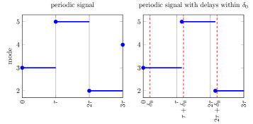
Figure 2: Periodic switching signals, with and without delays.

Remark 2.3

Our results rely on $\delta_{0}<\tau$, which we believe is a reasonable assumption. For example, in automotive applications, common switching periods are 4–8 milliseconds while jitters arising from CAN (Controller Area Networking) latency can be bounded by 120 microseconds.

In this paper we focus on periodic switched systems with switching delays, and their difference from those without switching delays. More specifically, we consider two switched systems

$$\Sigma_{\tau,\delta_{0}} =(\mathbb{R}^{n},P,{\mathcal{P}}_{\tau,\delta_{0}},F) \tau \leq\delta_{0}$$ -periodic with delays (1)

$$\Sigma_{\tau} =(\mathbb{R}^{n},P,{\mathcal{P}}_{\tau},F) \tau$$ -periodic

that have $\mathbb{R}^{n}$, $P$ and $F$ in common. For the former system $\Sigma_{\tau,\delta_{0}}$, the set ${\mathcal{P}}_{\tau,\delta_{0}}$ consists of all $\tau$-periodic signals with delays within $\delta_{0}$; for the latter system $\Sigma_{\tau}$ the set ${\mathcal{P}}_{\tau}$ consists of all $\tau$-periodic switching signals.

3 Transition Systems and Approximate Bisimulation

We use approximate bisimulations from Girard and Pappas (2007) to formalize proximity between $\Sigma_{\tau,\delta_{0}}$ (with delay) and $\Sigma_{\tau}$ (without). In this section we present our key definition (Def. 3.3) that allows such use of approximate bisimulation, in addition to a quick recap of a basic theory of approximate bisimulation.

Definition 3.1 (transition system)

A transition system is a triple $T=(Q,L,\autorightarrow{\scriptsize\raisebox{-3.31529pt}[0.0pt][0.0pt]{$$}}{\scriptsize\raisebox{3.31529pt}[0.0pt][0.0pt]{$$}},O,H,I)$, where

• $Q$ is a set of states;

• $L$ is a set of labels;

• $\autorightarrow{\scriptsize\raisebox{-3.31529pt}[0.0pt][0.0pt]{$$}}{\scriptsize\raisebox{3.31529pt}[0.0pt][0.0pt]{$$}}\subseteq Q\times L\times Q$ is a transition relation;

• $O$ is a set of outputs;

• $H:Q\rightarrow O$ is an output function; and

• $I\subseteq Q$ is a set of initial states.

We let $q\autorightarrow{\scriptsize\raisebox{-3.31529pt}[0.0pt][0.0pt]{$l$}}{\scriptsize\raisebox{3.31529pt}[0.0pt][0.0pt]{$$}}q^{\prime}$ denote the fact that $(q,l,q^{\prime})\in\autorightarrow{\scriptsize\raisebox{-3.31529pt}[0.0pt][0.0pt]{$$}}{\scriptsize\raisebox{3.31529pt}[0.0pt][0.0pt]{$$}}$.

In this paper, for a set $X$, a function $d:X\times X\rightarrow\mathbb{R}^{+}\cup\{\infty\}$ that satisfies, for all $x,y,z\in X$, $d(x,y)\geq 0$ and $d(x,z)\leq d(x,y)+d(y,z)$ is called a premetric on $X$. A transition system $T$ is said to be premetric if the set $O$ of outputs is equipped with a premetric $d$.

Approximate bisimulations are defined between transitions systems. It is a (co)inductive construct that guarantees henceforth proximity of behaviors of two states.

Definition 3.2

Let $T_{i}=(Q_{i},L,\autorightarrow{\scriptsize\raisebox{-3.31529pt}[0.0pt][0.0pt]{$$}}{\scriptsize\raisebox{3.31529pt}[0.0pt][0.0pt]{$i$}},O,H_{i},I_{i})$ ($i=1$, $2$) be two premetric transition systems, sharing the same sets of actions $L$ and outputs $O$ with a premetric $d$. Let $\varepsilon\in\mathbb{R}^{+}$ be a positive number; we call it a precision. A relation $R\subseteq Q_{1}\times Q_{2}$ is called an $\varepsilon$-approximate bisimulation relation between $T_{1}$ and $T_{2}$ if the following three conditions hold for all $(q_{1},q_{2})\in R$.

• $d(H_{1}(q_{1}),H_{2}(q_{2}))\leq\varepsilon$;

• $\forall q_{1}\autorightarrow{\scriptsize\raisebox{-3.31529pt}[0.0pt][0.0pt]{$l$}}{\scriptsize\raisebox{3.31529pt}[0.0pt][0.0pt]{$1$}}q^{\prime}_{1},\exists q_{2}\autorightarrow{\scriptsize\raisebox{-3.31529pt}[0.0pt][0.0pt]{$l$}}{\scriptsize\raisebox{3.31529pt}[0.0pt][0.0pt]{$2$}}q^{\prime}_{2}\text{ such that }(q^{\prime}_{1},q^{\prime}_{2})\in R$; and

• $\forall q_{2}\autorightarrow{\scriptsize\raisebox{-3.31529pt}[0.0pt][0.0pt]{$l$}}{\scriptsize\raisebox{3.31529pt}[0.0pt][0.0pt]{$2$}}q^{\prime}_{2},\exists q_{1}\autorightarrow{\scriptsize\raisebox{-3.31529pt}[0.0pt][0.0pt]{$l$}}{\scriptsize\raisebox{3.31529pt}[0.0pt][0.0pt]{$1$}}q^{\prime}_{1}\text{ such that }(q^{\prime}_{1},q^{\prime}_{2})\in R$.

The transition systems $T_{1}$ and $T_{2}$ are approximately bisimilar with precision $\varepsilon$ if there exists an $\varepsilon$-approximate bisimulation relation $R$ that satisfies the following conditions:

• $\forall q_{1}\in I_{1},\exists q_{2}\in I_{2}\text{ such that }(q_{1},q_{2})\in R$;

• $\forall q_{2}\in I_{2},\exists q_{1}\in I_{1}\text{ such that }(q_{1},q_{2})\in R$.

We let $T_{1}\sim_{\varepsilon}T_{2}$ denote the fact that $T_{1}$ and $T_{2}$ are approximately bisimilar with precision $\varepsilon$.

For the two switched systems $\Sigma_{\tau,\delta_{0}}=(\mathbb{R}^{n},P,{\mathcal{P}}_{\tau,\delta_{0}},F)$ and $\Sigma_{\tau}=(\mathbb{R}^{n},P,{\mathcal{P}}_{\tau},F)$ in (1), we shall construct associated transition systems $T(\Sigma_{\tau,\delta_{0}})$ and $T(\Sigma_{\tau})$, respectively.

Definition 3.3 ($T(\Sigma_{\tau,\delta_{0}}),T(\Sigma_{\tau})$)

The transition system

$$T(\Sigma_{\tau,\delta_{0}})=(Q_{\tau,\delta_{0}},L,\autorightarrow{\scriptsize\raisebox{-3.31529pt}[0.0pt][0.0pt]{$$}}{\scriptsize\raisebox{3.31529pt}[0.0pt][0.0pt]{$\tau,\delta_{0}$}},O,H_{\tau,\delta_{0}},I)\enspace,$$

associated with the switched system $\Sigma_{\tau,\delta_{0}}$ with delays in (1), is defined as follows:

• the set of states is $Q_{\tau,\delta_{0}}\vcentcolon=\mathbb{R}^{n}\times\bigcup_{k\in\mathbb{N}}[k\tau,k\tau+\delta_{0}]\times P$;

• the set of labels $L$ is the set of modes, i.e. $L\vcentcolon=P$;

• the transition relation $\autorightarrow{\scriptsize\raisebox{-3.31529pt}[0.0pt][0.0pt]{$$}}{\scriptsize\raisebox{3.31529pt}[0.0pt][0.0pt]{$\tau,\delta_{0}$}}\subseteq Q_{\tau,\delta_{0}}\times L\times Q_{\tau,\delta_{0}}$ is defined by $(x,t,p)\autorightarrow{\scriptsize\raisebox{-3.31529pt}[0.0pt][0.0pt]{$p^{\prime\prime}$}}{\scriptsize\raisebox{3.31529pt}[0.0pt][0.0pt]{$\tau,\delta_{0}$}}(x^{\prime},t^{\prime},p^{\prime})$ if $p=p^{\prime\prime}$, $x^{\prime}=\mathbf{x}(t^{\prime}-t,x,p)$ and there exists $k\in\mathbb{N}$ such that $t\in[k\tau,k\tau+\delta_{0}]$ and $t^{\prime}\in[(k+1)\tau,(k+1)\tau+\delta_{0}]$;

• the set of outputs is $O\vcentcolon=\mathbb{R}^{n}\times\mathbb{R}^{+}\times P$;

• the output function $H\colon Q_{\tau,\delta_{0}}\to O$ is the canonical embedding function $\mathbb{R}^{n}\times\bigcup_{k\in\mathbb{N}}[k\tau,k\tau+\delta_{0}]\times P\to\mathbb{R}^{n}\times\mathbb{R}^{+}\times P$; and

• the set of initial states is $I\vcentcolon=\mathbb{R}^{n}\times\{0\}\times P$.

Intuitively, each state $(x,t,p)$ of $T(\Sigma_{\tau,\delta_{0}})$ marks switching in the system $\Sigma_{\tau,\delta_{0}}$: $x\in\mathbb{R}^{n}$ is the (continuous) state at switching; $t$ is time of switching; and $p$ is the next mode. Note that, by the assumption on $\Sigma_{\tau,\delta_{0}}$, $t$ necessarily belongs to the interval $[k\tau,k\tau+\delta_{0}]$ for some $k\in\mathbb{N}$.

The transition system

$$T(\Sigma_{\tau}) =(Q_{\tau},L,\autorightarrow{\scriptsize\raisebox{-3.31529pt}[0.0pt][0.0pt]{$$}}{\scriptsize\raisebox{3.31529pt}[0.0pt][0.0pt]{$\tau$}},O,H_{\tau},I)\enspace,$$

associated with the switched system $\Sigma_{\tau}$ without delays in (1), is defined similarly, by fixing $\delta_{0}$ in the above definition to $0$.

Note that, in both of $T(\Sigma_{\tau,\delta_{0}})$ and $T(\Sigma_{\tau})$, the label $p^{\prime\prime}$ for a transition is uniquely determined by the mode component $p$ of the transition’s source $(x,t,p)$. Therefore, mathematically speaking, we do not need transition labels.

In Girard et al. (2010), the state space $Q$ of the transition system is just the continuous state space $\mathbb{R}^{n}$ of the switched system. In comparison, ours has two additional components, namely time $t$ and the current mode $p$. It is notable that moving a mode $p$ from transition labels to state labels allows us to analyze what happens during switching delays, that is, when the system keeps operating under the mode $p$ while it is not supposed to do so.

Definition 3.4 (premetric on outputs)

The transition systems $T(\Sigma_{\tau,\delta_{0}})$ and $T(\Sigma_{\tau})$ are premetric with the following $d$, defined on the common set of outputs $O=\mathbb{R}^{n}\times\mathbb{R}^{+}\times P$:

$$d((x,t,p),(x^{\prime},t^{\prime},p^{\prime}))\vcentcolon=$$

$$\left\{\begin{array}[]{ll}\|x-\mathbf{x}(t-t^{\prime},x^{\prime},p)\|&\begin{array}[]{ll}\text{if }p=p^{\prime},t^{\prime}=k\tau\text{ and }\\ \quad t\in[t^{\prime},t^{\prime}+\delta_{0}]\text{ for some }k\in\mathbb{N}\end{array}\\ \infty&\text{\ otherwise.}\end{array}\right.$$

4 Incremental Stability

After the pioneering work by Pola et al. (2008), a number of frameworks rely on the assumption of incremental stability for the construction of approximate bisimulations. Intuitively, a dynamical system is incrementally stable if, under any choice of an initial state, the resulting trajectory asymptotically converges to one reference trajectory. In this section, we review an incremental stability for switched systems, following Girard et al. (2010).

In the subsequent definitions we will be using the following classes of functions. A continuous function $\gamma:\mathbb{R}^{+}\rightarrow\mathbb{R}^{+}$ is a class ${\mathcal{K}}$ function if it is strictly increasing and $\gamma(0)=0$. A ${\mathcal{K}}$ function is a ${\mathcal{K}}_{\infty}$ function if $\gamma(x)\rightarrow\infty$ when $x\rightarrow\infty$. A continuous function $\beta:\mathbb{R}^{+}\times\mathbb{R}^{+}\rightarrow\mathbb{R}^{+}$ is a class ${\mathcal{KL}}$ function if 1) the function defined by $x\mapsto\beta(x,t)$ is a ${\mathcal{K}}_{\infty}$ function for any fixed $t$; and 2) for any fixed $x$, the function defined by $t\mapsto\beta(x,t)$ is strictly decreasing, and $\beta(x,t)\rightarrow 0$ when $t\rightarrow\infty$.

Definition 4.1

Let $\Sigma=(\mathbb{R}^{n},P,{\mathcal{P}},F)$ be a switched system. $\Sigma$ is said to be incrementally globally uniformly asymptotically stable ($\delta$-GUAS) if there exists a ${\mathcal{KL}}$ function $\beta$ such that the following holds for all $x,y\in\mathbb{R}^{n}$, $t\in\mathbb{R}^{+}$ and $\mathbf{p}\in{\mathcal{P}}$.

$$\|\mathbf{x}(t,x,\mathbf{p})-\mathbf{x}(t,y,\mathbf{p})\|\leq\beta(\|x-y\|,t)$$

Directly establishing that a system is $\delta$-GUAS is often hard. A usual technique in the field is to let a Lyapunov-type function play the role of witness for $\delta$-GUAS.

Definition 4.2

Let $\Sigma=(\mathbb{R}^{n},P,{\mathcal{P}},F)$ be a single-mode switched system with $P=\{p\}$. A smooth function $V:\mathbb{R}^{n}\times\mathbb{R}^{n}\rightarrow\mathbb{R}^{+}$ is a $\delta$-GAS Lyapunov function for $\Sigma$ if there exist ${\mathcal{K}}_{\infty}$ functions $\underline{\alpha}$, $\overline{\alpha}$ and $\kappa>0$ such that the following hold for all $x,y\in\mathbb{R}^{n}$.

$$\underline{\alpha}(\|x-y\|)\leq V(x,y)\leq\overline{\alpha}(\|x-y\|)$$ (2)

$$\frac{\partial V}{\partial x}(x,y)f_{p}(x)+\frac{\partial V}{\partial y}(x,y)f_{p}(y)\leq-\kappa V(x,y)$$ (3)

Note that the left-hand side of (3) is much like the Lie derivative of $V$ along the vector field $f_{p}$.

A sufficient condition for a switched system to be $\delta$-GUAS is the existence of a common $\delta$-GAS Lyapunov function.

Theorem 4.3 (Girard et al. (2010))

Let $\Sigma$ be a switched system. Assume that all continuous subsystems $\Sigma_{p}(p\in{\mathcal{P}})$ have a $\delta$-GAS Lyapunov function $V$ in common (with the same $\kappa$). Then, $V$ is called a common $\delta$-GAS Lyapunov function for $\Sigma$, and $\Sigma$ is $\delta$-GUAS.

Another sufficient condition is the existence of multiple $\delta$-GAS Lyapunov functions, under an additional assumption on the set of switching signals. The use of multiple Lyapunov functions for hybrid and switched systems is first advocated in Branicky (1998). We let ${\mathcal{S}}_{\tau_{d}}(\mathbb{R}^{+},P)\subseteq{\mathcal{S}}(\mathbb{R}^{+},P)$ denote the set of switching signals with a dwell time $\tau_{d}>0$, which means that the intervals between switching times are always longer than $\tau_{d}$.

We introduce the following notations. Given a switched system $\Sigma=(\mathbb{R}^{n},P=\{1,2,\cdots,m\},{\mathcal{P}},F)$, assume that, for each $p\in\{1,2,\dotsc,m\}$, we have a $\delta$-GAS Lyapunov function $V_{p}$ for the subsystem $\Sigma_{p}$. Then there exist a constant $\kappa_{p}\in\mathbb{R}^{+}$ and two ${\mathcal{K}}_{\infty}$ functions $\underline{\alpha}_{p}$ and $\overline{\alpha}_{p}$ as in Def. 4.2. Let us now define

$$\begin{array}[]{ll}\underline{\alpha}\vcentcolon=\min(\underline{\alpha}_{1},\dotsc,\underline{\alpha}_{m})\enspace,&\overline{\alpha}\vcentcolon=\max(\overline{\alpha}_{1},\dotsc,\overline{\alpha}_{m})\enspace,\\ \kappa\vcentcolon=\min(\kappa_{1},\dotsc,\kappa_{m})\enspace.\end{array}$$ (4)

Theorem 4.4 (Girard et al. (2010))

Let $\Sigma=(\mathbb{R}^{n},P,{\mathcal{P}},F)$ be a switched system. Assume that $P=\{1,2,\dotsc,m\}$, and that its set ${\mathcal{P}}$ of switching signals satisfies ${\mathcal{P}}\subseteq{\mathcal{S}}_{\tau_{d}}(\mathbb{R}^{+},P)$. Assume further that, for each $p\in P$, there exists a $\delta$-GAS Lyapunov function $V_{p}$ for the subsystem $\Sigma_{p}$. We also assume that there exists $\mu\in\mathbb{R}^{+}$ such that

$$V_{p}(x,y)\leq\mu V_{p^{\prime}}(x,y)\quad\text{for all }x,y\in\mathbb{R}^{n}\text{ and }p,p^{\prime}\in P.$$

If the dwell time $\tau_{d}$ satisfies $\tau_{d}>\frac{\log\mu}{\kappa}$, then $\Sigma_{\tau_{d}}$ is $\delta$-GUAS.

5 Approximate Bisimulation for Delays I: Common Lyapunov Functions

We have reviewed two witness notions for the incremental stability notion of $\delta$-GUAS: common and multiple $\delta$-GAS Lyapunov functions. These two notions have been previously used mainly for discrete-state abstraction of switched systems (see §8).

It is our main contribution to use the same incremental stability assumptions to derive upper bounds for errors caused by switching delays. We focus on periodic switching systems; our translation of them to transition systems (Def. 3.3) plays an essential role.

The use of common $\delta$-GAS Lyapunov functions is described in this section; the use of multiple $\delta$-GAS Lyapunov functions is in the next section. The proofs in both sections are omitted. See Appendix A for their proofs.

We will be using the following assumption.

Assumption 5.1 (bounded intermode derivative)

Let $\Sigma=(\mathbb{R}^{n},P,{\mathcal{P}},F)$ be a switched system, with $P=\{1,2,\dotsc,m\}$ and $F=\{f_{1},f_{2},\dotsc,f_{m}\}$ being the set of vector fields associated with each mode. We say a function $V\colon\mathbb{R}^{n}\times\mathbb{R}^{n}\rightarrow\mathbb{R}^{+}$ has bounded intermode derivatives if there exists a real number $\nu\geq 0$ such that, for any $p,p^{\prime}\in P$ that are distinct ($p\neq p^{\prime}$), the inequality

$$\frac{\partial V}{\partial x}(x,y)f_{p}(x)+\frac{\partial V}{\partial y}(x,y)f_{p^{\prime}}(y)\leq\nu$$ (5)

holds for each $x,y\in\mathbb{R}^{n}$.

Remark 5.2

Assumption 5.1 seems to be new: it is not assumed in the previous works on approximate bisimulation for switched systems. Imposing the assumption on $\delta$-GAS Lyapunov functions, however, is not a severe restriction. In Girard et al. (2010) they make the assumption

$$\exists\gamma\in\mathbb{R}^{+}.\;\forall x,y,z\in\mathbb{R}^{n}.\;|V(x,y)-V(x,z)|\leq\gamma(\|y-z\|)$$ (6)

(we do not need this assumption in the current work). It is claimed in Girard et al. (2010) that (6) is readily guaranteed if the dynamics of the switched system is confined to a compact set $C\subseteq\mathbb{R}^{n}$, and if $V$ is class $\mathcal{C}^{1}$ in the domain $C$. We can use the same compactness argument to ensure Assumption 5.1.

Definition 5.3 (the function $V^{\prime}$)

Let $\Sigma=(\mathbb{R}^{n},P,{\mathcal{P}},F)$ be a switched system, and let $V\colon\mathbb{R}^{n}\times\mathbb{R}^{n}\rightarrow\mathbb{R}^{+}$ be a common $\delta$-GAS Lyapunov function for $\Sigma$.

We define a function $V^{\prime}:(\mathbb{R}^{n}\times\mathbb{R}^{+}\times P)\times(\mathbb{R}^{n}\times\mathbb{R}^{+}\times P)\rightarrow\mathbb{R}^{+}$ in the following manner:

$$V^{\prime}\bigl{(}(x,t,p),(x^{\prime},t^{\prime},p^{\prime})\bigr{)}\vcentcolon=$$

$$\qquad\begin{cases}V\bigl{(}x,\mathbf{x}(t-t^{\prime},x^{\prime},p^{\prime})\bigr{)}&\text{ if }p=p^{\prime}\text{ and }t\in[t^{\prime},t^{\prime}+\delta_{0}]\\ \infty&\text{ otherwise.}\end{cases}$$

Recall that $\mathbf{x}(t-t^{\prime},x^{\prime},p^{\prime})$ is the state reached from $x^{\prime}$ after time $t-t^{\prime}$ following the vector field $f_{p^{\prime}}$.

Here is our main technical lemma.

Lemma 5.4

Let $\Sigma_{\tau}=(\mathbb{R}^{n},P,{\mathcal{P}}_{\tau},F)$ be a $\tau$-periodic switched system, and $\Sigma_{\tau,\delta_{0}}=(\mathbb{R}^{n},P,{\mathcal{P}}_{\tau,\delta_{0}},F)$ be a $\tau$-periodic switched system with delays within $\delta_{0}$. Assume that there exists a common $\delta$-GAS Lyapunov function $V$ for $\Sigma_{\tau}$, and that $V$ satisfies the additional assumption in Assumption 5.1.

We consider a relation $R_{\varepsilon}\subseteq(\mathbb{R}^{n}\times\mathbb{R}^{+}\times P)\times(\mathbb{R}^{n}\times\mathbb{R}^{+}\times P)$ defined by

$$(q,q^{\prime})\in R_{\varepsilon}\;\overset{\mathrm{def.}}{\Longleftrightarrow}\;V^{\prime}(q,q^{\prime})\leq\underline{\alpha}(\varepsilon)\enspace.$$ (7)

Here $V^{\prime}$ is from Def. 5.3. If we fix $\varepsilon=\underline{\alpha}^{-1}\left(\frac{\nu\delta_{0}}{1-e^{-\kappa(\tau-\delta_{0})}}\right)$ where $\nu$ is from Assumption 5.1, then, the relation $R_{\varepsilon}$ is an approximate bisimulation between the transition systems $T(\Sigma_{\tau,\delta_{0}})$ and $T(\Sigma_{\tau})$.

In the following theorem, we compare the trajectories of $\Sigma_{\tau,\delta_{0}}$ and $\Sigma_{\tau}$ from the same initial state $x$. It is a direct consequence from the previous lemma.

Theorem 5.5

Assume the same assumptions as in Lem. 5.4. Let $\mathbf{p}_{\tau}$ be a $\tau$-periodic switching signal, and $\mathbf{p}_{\tau,\delta_{0}}$ be the same signal but with delays within $\delta_{0}$. That is, for each $s\in\mathbb{R}^{+}$,

$$\mathbf{p}_{\tau,\delta_{0}}(s)=\begin{cases}\mathbf{p}_{\tau}(s)\text{ or }\mathbf{p}_{\tau}(s-\delta_{0})&\text{if $s\in\bigcup_{k\in\mathbb{N},k\geq 1}[k\tau,k\tau+\delta_{0})$}\\ \mathbf{p}_{\tau}(s)&\text{otherwise.}\end{cases}$$

We have, for each $t\in\mathbb{R}^{+}$,

$$\bigl{\|}\mathbf{x}(t,x,\mathbf{p}_{\tau,\delta_{0}})-\mathbf{x}(t,x,\mathbf{p}_{\tau})\bigr{\|}\;\leq\;\underline{\alpha}^{-1}\left(\frac{\nu\delta_{0}}{1-e^{-\kappa(\tau-\delta_{0})}}\right)\enspace.$$

Note that, for any desired precision $\varepsilon$, there always exists a small enough delay bound $\delta_{0}$ that achieves the precision $\varepsilon$ (i.e. $\frac{\nu\delta_{0}}{1-e^{-\kappa(\tau-\delta_{0})}}\leq\varepsilon$).

Remark 5.6

It turns out that the upper bound $\overline{\alpha}$ of a $\delta$-GAS Lyapunov function $V$ (see (2)) is not used in the above results nor their proofs. In Girard et al. (2010), $\overline{\alpha}$ is used to define the state space discretization parameter $\eta$ so that, for each initial state $q_{1}\in I_{1}$, there would be an approximately bisimilar initial state in $I_{2}$ and vice versa. This is not necessary in our current setting where there is an obvious correspondence between the initial states. That $\overline{\alpha}$ is unnecessary is also the case with the multiple Lyapunov function case in the next section.

6 Approximate Bisimulation for Delays II: Multiple Lyapunov Functions

We investigate the use of another witness for $\delta$-GUAS incremental stability—namely multiple $\delta$-GAS Lyapunov functions, see §4—for bounding errors caused by switching delays.

The following is an analogue of Assumption 5.1.

Assumption 6.1

Let $\Sigma=(\mathbb{R}^{n},P,{\mathcal{P}},F)$ be a switched system with $P=\{1,2,\dotsc,m\}$. Let $V_{1},\dotsc,V_{m}\colon\mathbb{R}^{n}\times\mathbb{R}^{n}\rightarrow\mathbb{R}^{+}$ be smooth functions. We say the functions $V_{1},\dotsc,V_{m}$ have bounded intermode derivatives if there exists a real number $\nu^{\prime}\geq 0$ such that, for each $p,p^{\prime}\in P$ that are distinct ($p\neq p^{\prime}$), the inequality

$$\frac{\partial V_{p^{\prime}}}{\partial x}(x,y)f_{p}(x)+\frac{\partial V_{p^{\prime}}}{\partial y}(x,y)f_{p^{\prime}}(y)\leq\nu^{\prime}$$ (8)

holds for each $x,y\in\mathbb{R}^{n}$. (Note the occurrences of $p$ and $p^{\prime}$.)

Under Assumption 6.1 and the dwell-time assumption, namely, $\tau-\delta_{0}>\frac{\log\mu}{\kappa}$, we can establish an approximate bisimulation between the transition systems $T(\Sigma_{\tau,\delta_{0}})$ and $T(\Sigma_{\tau})$.

Lemma 6.2

Let $\Sigma_{\tau}=(\mathbb{R}^{n},P,{\mathcal{P}}_{\tau},F)$ be a $\tau$-periodic switched system and $\Sigma_{\tau,\delta_{0}}=(\mathbb{R}^{n},P,{\mathcal{P}}_{\tau,\delta_{0}},F)$ be a $\tau$-periodic switched system with delays within $\delta_{0}$. Assume that for each $p\in P$, there is a $\delta$-GAS Lyapunov function $V_{p}$ for the single-mode subsystem $\Sigma_{\tau,p}$. We also assume Assumption 6.1 for $V_{1},\dotsc,V_{m}$, and that there exists $\mu\in\mathbb{R}^{+}$ such that

$$V_{p}(x,y)\leq\mu V_{p^{\prime}}(x,y)\;\text{for all }x,y\in\mathbb{R}^{n}\text{ and }p,p^{\prime}\in P\enspace.$$ (9)

The last assumption is the same as in Thm. 4.4. Additionally, we assume the dwell-time assumption $\tau-\delta_{0}>\frac{\log\mu}{\kappa}$.

We consider a relation $R_{\varepsilon}\subseteq(\mathbb{R}^{n}\times\mathbb{R}^{+}\times P)\times(\mathbb{R}^{n}\times\mathbb{R}^{+}\times P)$ defined by

$$(q,q^{\prime})\in R_{\varepsilon}\;\overset{\mathrm{def.}}{\Longleftrightarrow}\;V^{\prime}(q,q^{\prime})\leq\underline{\alpha}(\varepsilon)\enspace.$$ (10)

Here the function $V^{\prime}$ is defined as follows, adapting Def. 5.3 to the current multiple Lyapunov function setting.

$$V^{\prime}\bigl{(}(x,t,p),(x^{\prime},t^{\prime},p^{\prime})\bigr{)}\vcentcolon=$$

$$\qquad\begin{cases}V_{p}\bigl{(}x,\mathbf{x}(t-t^{\prime},x^{\prime},p^{\prime})\bigr{)}&\text{ if }p=p^{\prime}\text{ and }t\in[t^{\prime},t^{\prime}+\delta_{0}]\\ \infty&\text{ otherwise.}\end{cases}$$

If we fix $\varepsilon=\underline{\alpha}^{-1}\left(\frac{\nu\delta_{0}}{1-\mu e^{-\kappa(\tau-\delta_{0})}}\right)$ where $\underline{\alpha}$ and $\kappa$ are from (4) and $\nu^{\prime}$ is from Assumption 6.1, then, the relation $R_{\varepsilon}$ is an approximate bisimulation between the transition systems $T(\Sigma_{\tau,\delta_{0}})$ and $T(\Sigma_{\tau})$.

The next result follows directly from Lem. 6.2.

Theorem 6.3

Assume the same assumptions as in Lem. 6.2, and let $\mathbf{p}_{\tau}$ and $\mathbf{p}_{\tau,\delta_{0}}$ be those periodic switching signals, without and with delays, as in Thm. 5.5. If $\tau-\delta_{0}>\frac{\log\mu}{\kappa}$, we have, for each $t\in\mathbb{R}^{+}$,

$$\bigl{\|}\mathbf{x}(t,x,\mathbf{p}_{\tau,\delta_{0}})-\mathbf{x}(t,x,\mathbf{p}_{\tau})\bigr{\|}\leq\underline{\alpha}^{-1}\left(\frac{\nu^{\prime}\delta_{0}}{1-\mu e^{-\kappa(\tau-\delta_{0})}}\right)\enspace.$$

7 Example

We demonstrate our framework using the example of the boost DC-DC converter from Beccuti et al. (2005). It is a common example of switched systems. For this example we have a common $\delta$-GAS Lyapunov function $V$, and therefore we appeal to the results in §5. We also demonstrate the control synthesis workflow in Fig. 1.

Another example of a water tank with nonlinear dynamics is presented in Appendix B. It has multiple $\delta$-GAS Lyapunov functions, and we use the results in §6.

System Description

The system we consider is the boost DC-DC converter in Fig. 3. It is taken from Beccuti et al. (2005); here we follow and extend the analysis in Girard et al. (2010). The circuit includes a capacitor with capacitance $x_{c}$ and an inductor with inductance $x_{l}$. The capacitor has the equivalent series resistance $r_{c}$, and the inductor has the internal resistance $r_{l}$. The input voltage is $v_{s}$, and the resistance $r_{o}$ is the output load resistance. The state $x(t)=\begin{bmatrix}i_{l}(t)\\ v_{c}(t)\end{bmatrix}$ of this system consists of the inductor current $i_{l}$ and the capacitor voltage $v_{c}$.

The dynamics of this system has two modes $\{{\textit{ON}},{\textit{OFF}}\}$, depending on whether the switch in the circuit is on or off. By elementary circuit theory, the dynamics in each mode is modeled by

$$\dot{x}(t)=A_{p}x(t)+b\quad\text{for }p\in\{{\textit{ON}},{\textit{OFF}}\}\enspace,\text{ where}$$

$$A_{{\textit{ON}}}=\begin{bmatrix}-\frac{r_{l}}{x_{l}}&0\\ 0&-\frac{1}{x_{c}(r_{o}+r_{c})}\end{bmatrix},\quad b=\begin{bmatrix}\frac{v_{s}}{x_{l}}\\ 0\end{bmatrix}\text{ and}$$

$$A_{{\textit{OFF}}}=\begin{bmatrix}-\frac{r_{l}r_{o}+r_{l}r_{c}+r_{o}r_{c}}{x_{l}(r_{o}+r_{c})}&-\frac{r_{l}r_{o}+r_{l}r_{c}+r_{o}r_{c}}{x_{l}(r_{o}+r_{c})}\\ \frac{r_{o}}{x_{c}(r_{o}+r_{c})}&-\frac{1}{x_{c}(r_{o}+r_{c})}\end{bmatrix}\enspace.$$

We use the parameter values from Beccuti et al. (2005), that is, $x_{c}=70$ p.u., $x_{l}=3$ p.u., $r_{c}=0.005$ p.u., $r_{l}=0.05$ p.u., $r_{o}=1$ p.u. and $v_{s}=1$ p.u.

Figure 3: The boost DC-DC converter circuit.

Analysis

Following Girard et al. (2010), we rescale the second variable of the system and redefine the state $x(t)=\begin{bmatrix}i_{l}(t)\\ 5v_{c}(t)\end{bmatrix}$ for better numerical conditioning. The ODEs are updated accordingly.

It is shown in Girard et al. (2010) that the dynamics in each mode is $\delta$-GAS. They share a common $\delta$-GAS Lyapunov function $V(x,y)=\sqrt{(x-y)^{T}M(x-y)}$, with $M=\begin{bmatrix}1.0224&0.0084\\ 0.0084&1.0031\end{bmatrix}$. The common Lyapunov function $V$ has $\underline{\alpha}(s)=s,\overline{\alpha}(s)=1.0127s$ and $\kappa=0.014$. This common Lyapunov function is discovered in Girard et al. (2010) via SDP optimization; we use the same function as an ingredient for our approximate bisimulation.

Our ultimate goal is to synthesize a switching signal that keeps the dynamics in a safe region $\mathcal{S}\vcentcolon=[1.3,1.7]\times[5.7,5.8]$. We shall follow the two-step workflow in Fig. 1.

Let us first use Thm. 5.5 and derive a bound $\varepsilon_{1}$ for errors caused by switching delays. We set the switching period $\tau=0.5$ and the maximum delay $\delta_{0}=\frac{\tau}{1000}$. On top of the analysis in Girard et al. (2010), we have to verify the condition we additionally impose (namely Assumption 5.1). Let us now assume that the dynamics stays in the safe region $\mathcal{S}=[1.3,1.7]\times[5.7,5.8]$—this assumption will be eventually discharged when we synthesize a safe controller. Then it is not hard to see that $\nu=0.41$ satisfies the inequality (5). By Thm. 5.5, we obtain that the error between $\Sigma_{\tau,\delta_{0}}$ (the boost DC-DC converter with delays) and $\Sigma_{\tau}$ (the one without delays) is bounded by $\varepsilon_{1}=0.0294176$.

We sketch how we can combine the above analysis with the analysis in Girard et al. (2010), in the way prescribed in Fig. 1. In Girard et al. (2010) they use the same Lyapunov function as above to derive a discrete symbolic model $T_{\tau}^{\text{symb}}$ and establish an approximate bisimulation between $T(\Sigma_{\tau})$ and the symbolic model. Their symbolic model $T_{\tau}^{\text{symb}}$ can be constructed so that any desired error bound $\varepsilon_{2}$ is guaranteed (a smaller $\varepsilon_{2}$ calls for a finer grid for discretization and hence a bigger symbolic model).

Now we employ an algorithm from supervisory control in Ramadge and Wonham (1987), and synthesize a set of safe switching signals that confine the dynamics of $T_{\tau}^{\text{symb}}$ to a shrunk safe region $\mathcal{S}_{\varepsilon_{1}+\varepsilon_{2}}\vcentcolon=[1.3+(\varepsilon_{1}+\varepsilon_{2}),1.7-(\varepsilon_{1}+\varepsilon_{2})]\times[5.7+(\varepsilon_{1}+\varepsilon_{2}),5.8-(\varepsilon_{1}+\varepsilon_{2})]$. Let $\mathbf{p}$ be any such safe switching signal. By the second approximate bisimulation in Fig. 1, the signal $\mathbf{p}$ is guaranteed to keep the dynamics of $\Sigma_{\tau}$ in the region $\mathcal{S}_{\varepsilon_{1}}\vcentcolon=[1.3+\varepsilon_{1},1.7-\varepsilon_{1}]\times[5.7+\varepsilon_{1},5.8-\varepsilon_{1}]$. Finally, the first approximate bisimulation in Fig. 1 guarantees that the signal $\mathbf{p}$ keeps the dynamics of $\Sigma_{\tau,\delta_{0}}$, the system with switching delays, in $\mathcal{S}$.

Remark 7.1

On the choice of a safe region used in control synthesis for the symbolic model $T_{\tau}^{\text{symb}}$, our current choice $\mathcal{S}_{\varepsilon_{1}+\varepsilon_{2}}\subsetneq\mathcal{S}$ is more conservative than the choice in Girard et al. (2010), where they in fact expand (rather than shrink) the original safe region $\mathcal{S}$. We believe our conservative choice is required in the current workflow (Fig. 1) where two approximation steps are totally separated. Tighter integration of the two steps can lead to relaxation of this conservative choice.

8 Related Work

The notion of approximate bisimulation is first introduced in Girard and Pappas (2007). Use of incremental stability as a source of approximate bisimulations is advocated in Pola et al. (2008). This useful technique has found its applications in a variety of system classes as well as in a variety of problems. A notable application is discretization of continuous state spaces so that discrete verification/synthesis techniques can be employed. The original framework in Pola et al. (2008) has seen its extension to switched systems (Girard et al. (2010)), systems with disturbance (Pola and Tabuada (2009)), and so on. A comprehensive framework where discrete control synthesis is integrated is presented in Girard (2010); the works discussed so far are nicely summarized in the overview paper by Girard and Pappas (2011).

A line of works relevant to ours addresses the issue of time delays (Pola et al. (2010b, a)). The work by Pola et al. (2010b) deals with fixed time delays and the one by Pola et al. (2010a) considers unknown time delays. The goal of these works, which is different from ours, is to construct a comprehensive symbolic (discretized) model that encompasses all possible delays and switching signals. In particular, possible delays are thought of as disturbances (i.e. demonic/adversarial nondeterminism) and consequently they use alternating approximate bisimulations. The main technical gadget in doing so is spline-based finitary approximation of continuous-time signals.

Towards control synthesis for switched systems with unknown switching delays, our workflow (Fig. 1) is two-step while a workflow based on Pola et al. (2010a) is one-step. The latter works as follows. The results in Pola et al. (2010a) yields a symbolic model for a switched system with delays; it is given by a two-player finite-state game $\mathcal{G}$ where angelic moves switching signals and demonic moves are time delays. By solving the game $\mathcal{G}$ (e.g. by the algorithm in Jurdzinski (2000)) one obtains a control strategy. It seems that our two-step workflow has an advantage in complexity: by collecting the spline-based approximations of all possible delays and switching signals, the game $\mathcal{G}$ in Pola et al. (2010a) tends to have a big number of transitions. It has to be noted, however, that the workflow following Pola et al. (2010a) applies to a greater variety of systems (than switched systems) and a resulting control strategy can be more fine-grained (reacting to delays, while our controller always assumes the worst time delays).

Another related work that refers to time delays is Liu and Ozay (2016). The biggest difference between Liu and Ozay (2016) and our work is that their framework is based on the invariance assumption of atomic formulas ($\delta$ in the paper): as long as errors due to delays do not exceed $\delta$, the system satisfies the same set of LTL formulas. In contrast, our results bound distances between trajectories; the use of such bounds is not restricted to satisfaction of LTL specifications.

The works Borri et al. (2012); Zamani et al. (2017) study symbolic abstraction of networked control systems, taking into accounts issues including time delays. The main difference from the current work is that their delays are assumed to be always multiples ($0,\tau,2\tau,\dotsc$) of the period $\tau$; this assumption is enforced in their framework by system components called the zero-order hold (ZOH). Their game-based frameworks are based on alternating approximate bisimulations, much like in Pola et al. (2010a), but the above assumption leads to simpler games for control synthesis. We note that our current setting—where delays are within a fixed bound $\delta_{0}$ with $\delta_{0}<\tau$—is outside the scope of Borri et al. (2012); Zamani et al. (2017).

A recent line of works by Khatib et al. (2016, 2017) tackles the challenge of time delays too. They take timing contracts as specifications; and study a verification problem (Khatib et al. (2016)), and a scheduling problem under the single-processor multiple-task setting (Khatib et al. (2017)). A crucial difference from the current work is that they assume linear dynamics, while we can deal with nonlinear dynamics (under the assumption of incremental stability).

The works by Abbas et al. (2014); Abbas and Fainekos (2015) present an alternative notion of proximity between trajectories called $(\tau,\varepsilon)$-closeness. Its intuition is that, in establishing that the distance between two trajectories is within $\varepsilon$, it is allowed to shift time by $\tau$. Adapting our current results to this notion of proximity does not seem hard, by modifying the definitions in Def. 3.4 and 5.3.

9 Conclusions and Future Work

In this paper, we introduced an approximate bisimulation framework and provided upper bounds for errors that arise from switching delays in periodic switched systems. Our focus on switched systems allows us to use the same incremental stability notion ($\delta$-GUAS) as in Girard et al. (2010) as an ingredient for an approximate bisimulation. This is an advantage in the control synthesis workflow (Fig. 1) for switched systems with delays, in which we separate two concerns of time delays and discretization of state spaces.

Adaptation of the current framework to $(\tau,\varepsilon)$-closeness in Abbas et al. (2014); Abbas and Fainekos (2015) is imminent future work. As we discussed in §8, this adaptation will not be hard.

Extending the current results to a wider class of systems beyond periodic switched ones is a direction that we shall pursue. In particular, we are interested in disturbances and the consequent use of alternating approximate bisimulation introduced in Pola and Tabuada (2009). Such an extension should be carefully devised so that the two-step workflow in Fig. 1 remain valid. For example, once the controller synthesized based on the symbolic model $T_{\tau}^{\text{symb}}$ involves sensing, it is unlikely that the controller achieves precision $\varepsilon_{1}+\varepsilon_{2}$ in the system $\Sigma_{\tau,\delta_{0}}$ with delays. In such a setting, errors in each of the two approximation steps in Fig. 1 can amplify each other, resulting in an overall error bound that is much worse than $\varepsilon_{1}+\varepsilon_{2}$. A related topic of future work is suggested in Rem. 7.1.

Appendix A Relaxation of approximate bisimulation for time-varying error bounds

In this appendix, we introduce a relaxed notion of approximate bisimulation to obtain a tighter error bound that can grow in time. We present the proofs for the lemmas and the theorems in this appendix. We do not show the omitted proofs for the results stated in §5 and §6 themselves, because they are direct consequences from the results in this appendix.

Our relaxation of approximate bisimulation allows errors to potentially grow after each transition, in a manner regulated by some increasing function $g\colon\mathbb{R}^{+}\to\mathbb{R}^{+}$.

Definition A.1 ($g$-incrementing approximate bisimulation)

Let $T_{i}=(Q_{i},L,\autorightarrow{\scriptsize\raisebox{-3.31529pt}[0.0pt][0.0pt]{$$}}{\scriptsize\raisebox{3.31529pt}[0.0pt][0.0pt]{$i$}},O,H_{i},I_{i})$ ($i=1$, $2$) be two premetric transition systems with premetric $d$; they share the same sets of actions $L$ and outputs $O$. Let $\varepsilon\in\mathbb{R}^{+}$ be a precision, and $g\colon\mathbb{R}^{+}\to\mathbb{R}^{+}$ be an increasing function.

A family $\{R_{\varepsilon}\}_{\varepsilon\geq 0}$ of relations $R_{\varepsilon}\subseteq Q_{1}\times Q_{2}$ indexed by $\varepsilon\geq 0$ is called a $g$-incrementing approximate bisimulation between $T_{1}$ and $T_{2}$ if the following conditions hold for all $\varepsilon\geq 0$ and for all $(q_{1},q_{2})\in R_{\varepsilon}$:

• $d(H_{1}(q_{1}),H_{2}(q_{2}))\leq\varepsilon$; and

• there exists a function $g$ such that

  • $\forall q_{1}\autorightarrow{\scriptsize\raisebox{-3.31529pt}[0.0pt][0.0pt]{$l$}}{\scriptsize\raisebox{3.31529pt}[0.0pt][0.0pt]{$1$}}q^{\prime}_{1},\exists q_{2}\autorightarrow{\scriptsize\raisebox{-3.31529pt}[0.0pt][0.0pt]{$l$}}{\scriptsize\raisebox{3.31529pt}[0.0pt][0.0pt]{$2$}}q^{\prime}_{2}\text{ s.t. }(q^{\prime}_{1},q^{\prime}_{2})\in R_{g(\varepsilon)}$;
    and

  • $\forall q_{2}\autorightarrow{\scriptsize\raisebox{-3.31529pt}[0.0pt][0.0pt]{$l$}}{\scriptsize\raisebox{3.31529pt}[0.0pt][0.0pt]{$2$}}q^{\prime}_{2},\exists q_{1}\autorightarrow{\scriptsize\raisebox{-3.31529pt}[0.0pt][0.0pt]{$l$}}{\scriptsize\raisebox{3.31529pt}[0.0pt][0.0pt]{$1$}}q^{\prime}_{1}\text{ s.t. }(q^{\prime}_{1},q^{\prime}_{2})\in R_{g(\varepsilon)}$.

We can establish a $g$-incrementing approximate bisimulation between the transition systems $T(\Sigma_{\tau,\delta_{0}})$ and $T(\Sigma_{\tau})$.

Lemma A.2

Let $\Sigma_{\tau}=(\mathbb{R}^{n},P,{\mathcal{P}}_{\tau},F)$ be a $\tau$-periodic switched system, and $\Sigma_{\tau,\delta_{0}}=(\mathbb{R}^{n},P,{\mathcal{P}}_{\tau,\delta_{0}},F)$ be a $\tau$-periodic switched system with delays within $\delta_{0}$. Assume that there exists a common $\delta$-GAS Lyapunov function $V$ for $\Sigma_{\tau}$, and that $V$ satisfies the additional assumption in Assumption 5.1. Then, for a suitable $g$, there exists a $g$-incrementing approximate bisimulation $\{R_{\varepsilon}\}_{\varepsilon\geq 0}$ between the transition systems $T(\Sigma_{\tau,\delta_{0}})$ and $T(\Sigma_{\tau})$.

Specifically, we define a function $g$ by

$$g(\varepsilon)\vcentcolon=\underline{\alpha}^{-1}\left(e^{-\kappa(\tau-\delta_{0})}\underline{\alpha}(\varepsilon)+\nu\delta_{0}\right)\enspace,$$

where $\nu$ is from Assumption 5.1. For each $\varepsilon\geq 0$, we define a relation $R_{\varepsilon}\subseteq(\mathbb{R}^{n}\times\mathbb{R}^{+}\times P)\times(\mathbb{R}^{n}\times\mathbb{R}^{+}\times P)$ by

$$(q,q^{\prime})\in R_{\varepsilon}\;\overset{\mathrm{def.}}{\Longleftrightarrow}\;V^{\prime}(q,q^{\prime})\leq\underline{\alpha}(\varepsilon)\enspace.$$ (11)

Here $V^{\prime}$ is from Def. 5.3.

It is obvious from the monotonicity of $\underline{\alpha}$ that $(q_{\tau,\delta_{0}},q_{\tau})\in R_{\varepsilon}$ implies $d(q_{\tau,\delta_{0}},q_{\tau})\leq\varepsilon$.

For $q_{\tau,\delta_{0}}=(x_{\tau,\delta_{0}},t_{\tau,\delta_{0}},p_{\tau,\delta_{0}})$ and $q_{\tau}=(x_{\tau},t_{\tau},p_{\tau})$, we assume that $q_{\tau,\delta_{0}}\autorightarrow{\scriptsize\raisebox{-3.31529pt}[0.0pt][0.0pt]{$l$}}{\scriptsize\raisebox{3.31529pt}[0.0pt][0.0pt]{$\tau,\delta_{0}$}}q_{\tau,\delta_{0}}^{\prime}=(x^{\prime}_{\tau,\delta_{0}},t^{\prime}_{\tau,\delta_{0}},p^{\prime}_{\tau,\delta_{0}})$ and $(q_{\tau,\delta_{0}},q_{\tau})\in R_{\varepsilon}$ for some $\varepsilon$. Our goal is to show that there exists $q_{\tau}^{\prime}=(x^{\prime}_{\tau},t^{\prime}_{\tau},p^{\prime}_{\tau})$ such that $q_{\tau}\autorightarrow{\scriptsize\raisebox{-3.31529pt}[0.0pt][0.0pt]{$l$}}{\scriptsize\raisebox{3.31529pt}[0.0pt][0.0pt]{$\tau$}}q_{\tau}^{\prime}$ and $(q_{\tau,\delta_{0}}^{\prime},q_{\tau}^{\prime})\in R_{g(\varepsilon)}$.

By the definition (11) of the relation $R_{\varepsilon}$ and the construction of the transition systems $T_{\tau,\delta_{0}}(\Sigma_{\tau,\delta_{0}})$ and $T_{\tau}(\Sigma_{\tau})$, it is easy to see that $p_{\tau,\delta_{0}}=p_{\tau}$, $t_{\tau}=k\tau$, $t_{\tau,\delta_{0}}\in[k\tau,k\tau+\delta_{0}]$ and $t^{\prime}_{\tau,\delta_{0}}\in[(k+1)\tau,(k+1)\tau+\delta_{0}]$ for some $k\in\mathbb{N}$. Then we define $q_{\tau}^{\prime}$ by $q_{\tau}^{\prime}=(\mathbf{x}(\tau,x_{\tau},p_{\tau}),(k+1)\tau,p^{\prime}_{\tau,\delta_{0}})$ to obtain $q_{\tau}\autorightarrow{\scriptsize\raisebox{-3.31529pt}[0.0pt][0.0pt]{$l$}}{\scriptsize\raisebox{3.31529pt}[0.0pt][0.0pt]{$\tau$}}q_{\tau}^{\prime}$.

Now we show $(q_{\tau,\delta_{0}}^{\prime},q_{\tau}^{\prime})\in R_{g(\varepsilon)}$ for this $q_{\tau}^{\prime}$. By the assumption $(q_{\tau,\delta_{0}},q_{\tau})\in R_{\varepsilon}$, we have $V^{\prime}(q_{\tau,\delta_{0}},q_{\tau})\leq\underline{\alpha}(\varepsilon)$, which means

$$V(x_{\tau,\delta_{0}},\mathbf{x}(t_{\tau,\delta_{0}}-t_{\tau},x_{\tau},p_{\tau}))\leq\underline{\alpha}(\varepsilon).$$ (12)

Note that this equation refers to the states of the two systems at $t=t_{\tau,\delta_{0}}$. When time progresses for $t_{\tau}^{\prime}-t_{\tau,\delta_{0}}$ with mode $p_{\tau,\delta_{0}}=p_{\tau}$ for both systems from $t=t_{\tau,\delta_{0}}$, we have

$$V(\mathbf{x}(t_{\tau}^{\prime}-t_{\tau,\delta_{0}},x_{\tau,\delta_{0}},p_{\tau}),\mathbf{x}(t_{\tau}^{\prime}-t_{\tau,\delta_{0}},\mathbf{x}(t_{\tau,\delta_{0}}-t_{\tau},x_{\tau},p_{\tau}),p_{\tau}))$$

$$\leq e^{-\kappa(t_{\tau}^{\prime}-t_{\tau,\delta_{0}})}V(x_{\tau,\delta_{0}},\mathbf{x}(t_{\tau,\delta_{0}}-t_{\tau},x_{\tau},p_{\tau}))$$

$$\leq e^{-\kappa(\tau-\delta_{0})}V(x_{\tau,\delta_{0}},\mathbf{x}(t_{\tau,\delta_{0}}-t_{\tau},x_{\tau},p_{\tau})).$$ (13)

Note that this equation refers to the states of the two systems at $t=t_{\tau}^{\prime}$. When time progresses for $t_{\tau,\delta_{0}}^{\prime}-t_{\tau}^{\prime}$ with mode $p_{\tau,\delta_{0}}(=p_{\tau})$ for $T_{\tau,\delta_{0}}(\Sigma_{\tau,\delta_{0}})$ and with mode $p^{\prime}_{\tau}$ for $T_{\tau}(\Sigma_{\tau}))$ from $t=t_{\tau}^{\prime}$, we have

$$\quad V^{\prime}(q^{\prime}_{\tau,\delta_{0}},q^{\prime}_{\tau})$$

$$=V(\mathbf{x}(t_{\tau,\delta_{0}}^{\prime}-t_{\tau}^{\prime},\mathbf{x}(t_{\tau}^{\prime}-t_{\tau,\delta_{0}},x_{\tau,\delta_{0}},p_{\tau}),p_{\tau}),$$

$$\qquad\mathbf{x}(t_{\tau,\delta_{0}}^{\prime}-t_{\tau}^{\prime},\mathbf{x}(t_{\tau}^{\prime}-t_{\tau,\delta_{0}},\mathbf{x}(t_{\tau,\delta_{0}}-t_{\tau},x_{\tau},p_{\tau}),p_{\tau}),p^{\prime}_{\tau}))$$

$$\leq e^{-\kappa(\tau-\delta_{0})}V(x_{\tau,\delta_{0}},\mathbf{x}(t_{\tau,\delta_{0}}-t_{\tau},x_{\tau},p_{\tau}))+\nu(t_{\tau,\delta_{0}}^{\prime}-t_{\tau}^{\prime})$$

$$\leq e^{-\kappa(\tau-\delta_{0})}V(x_{\tau,\delta_{0}},\mathbf{x}(t_{\tau,\delta_{0}}-t_{\tau},x_{\tau},p_{\tau}))+\nu\delta_{0}$$

$$=e^{-\kappa(\tau-\delta_{0})}V^{\prime}(q_{\tau,\delta_{0}},q_{\tau})+\nu\delta_{0}$$

$$\leq e^{-\kappa(\tau-\delta_{0})}\underline{\alpha}(\varepsilon)+\nu\delta_{0}$$

$$=\underline{\alpha}(g(\varepsilon)).$$ (14)

In the RHS of the first inequality in (14), the first term is from (13), which bounds the distance of the states at time $t^{\prime}_{\tau}$. The second term overapproximates the effect of the behavior from $t^{\prime}_{\tau}$ to $t^{\prime}_{\tau,\delta_{0}}$, when the two systems are operated in different modes.

Thus we have $(q_{\tau,\delta_{0}}^{\prime},q_{\tau}^{\prime})\in R_{g(\varepsilon)}$. The converse simulation condition is shown similarly.

Theorem A.3

Assume the same assumptions as in Lem. A.2. Let $\mathbf{p}_{\tau}$ be a $\tau$-periodic switching signal, and $\mathbf{p}_{\tau,\delta_{0}}$ be the same signal but with delays within $\delta_{0}$. That is, for each $s\in\mathbb{R}^{+}$,

$$\mathbf{p}_{\tau,\delta_{0}}(s)=\begin{cases}\mathbf{p}_{\tau}(s)\text{ or }\mathbf{p}_{\tau}(s-\delta_{0})&\text{if $s\in\bigcup_{k\in\mathbb{N},k\geq 1}[k\tau,k\tau+\delta_{0})$}\\ \mathbf{p}_{\tau}(s)&\text{otherwise.}\end{cases}$$

We have, for each $k\in\mathbb{N}$ and $t\in[k\tau,(k+1)\tau)$,

$$\bigl{\|}\mathbf{x}(t,x,\mathbf{p}_{\tau,\delta_{0}})-\mathbf{x}(t,x,\mathbf{p}_{\tau})\bigr{\|}\;\leq$$

$$\quad\underline{\alpha}^{-1}\left(\frac{\nu\delta_{0}}{1-e^{-\kappa(\tau-\delta_{0})}}+e^{-\kappa(\tau-\delta_{0})k}\left(-\frac{\nu\delta_{0}}{1-e^{-\kappa(\tau-\delta_{0})}}\right)\right)\enspace.$$

Lem. A.2 serves as a recurrence relation with respect to the number $k$ of switching. By solving it with the initial condition of $d(q_{\tau,\delta_{0},0},q_{\tau,0})=0$, we obtain the result of

$$d(q_{\tau,\delta_{0}},q_{\tau})$$

$$\leq \ g^{k}(0)$$

$$= \ \underline{\alpha}^{-1}\left(\frac{\nu\delta_{0}}{1-e^{-\kappa(\tau-\delta_{0})}}+e^{-\kappa(\tau-\delta_{0})k}\left(-\frac{\nu\delta_{0}}{1-e^{-\kappa(\tau-\delta_{0})}}\right)\right),$$

for all states $q_{\tau,\delta_{0}}$ and $q_{\tau}$ that can be reached via a same sequence of actions of length $k$.

Since the definition of the premetric $d$ is as Def. 3.4, this result only refers to the error between two systems at the switching time in $[k\tau,(k+1)\tau)$. It is easy, however, to have that this $\quad\underline{\alpha}^{-1}\left(\frac{\nu\delta_{0}}{1-e^{-\kappa(\tau-\delta_{0})}}+e^{-\kappa(\tau-\delta_{0})k}\left(-\frac{\nu\delta_{0}}{1-e^{-\kappa(\tau-\delta_{0})}}\right)\right)$ is actually an upper bound of $\bigl{\|}\mathbf{x}(t,x,\mathbf{p}_{\tau,\delta_{0}})-\mathbf{x}(t,x,\mathbf{p}_{\tau})\bigr{\|}$, for all $t\in[k\tau,(k+1)\tau)$, from $\kappa\geq 0$ and $\nu\geq 0$.

Note that the bound in Thm. A.3 can grow over time (i.e. over the number $k$ of switching), while the one in Thm. 5.5 is a conservative bound that is time-invariant.

The following lemma is for the multiple Lyapunov functions. Note that we do not need the dwell-time assumption, which is necessary to obtain the approximate bisimulation in Lem. 6.2.

Lemma A.4

Let $\Sigma_{\tau}=(\mathbb{R}^{n},P,{\mathcal{P}}_{\tau},F)$ be a $\tau$-periodic switched system and $\Sigma_{\tau,\delta_{0}}=(\mathbb{R}^{n},P,{\mathcal{P}}_{\tau,\delta_{0}},F)$ be a $\tau$-periodic switched system with delays within $\delta_{0}$. Assume that for each $p\in P$, there is a $\delta$-GAS Lyapunov function $V_{p}$ for the single-mode subsystem $\Sigma_{\tau,p}$. We also assume Assumption 6.1 for $V_{1},\dotsc,V_{m}$, and that there exists $\mu\in\mathbb{R}^{+}$ such that

$$V_{p}(x,y)\leq\mu V_{p^{\prime}}(x,y)\;\text{for all }x,y\in\mathbb{R}^{n}\text{ and }p,p^{\prime}\in P\enspace.$$ (15)

Then, for a suitable $g$, there exists a $g$-incrementing approximate bisimulation $\{R_{\varepsilon}\}_{\varepsilon\geq 0}$ between the transition systems $T(\Sigma_{\tau,\delta_{0}})$ and $T(\Sigma_{\tau})$.

Specifically, we define $g$ by

$$g(\varepsilon)\vcentcolon=\underline{\alpha}^{-1}\left(\mu e^{-\kappa(\tau-\delta_{0})}\underline{\alpha}(\varepsilon)+\nu^{\prime}\delta_{0}\right)\enspace,$$

where $\underline{\alpha}$ and $\kappa$ are from (4) and $\nu^{\prime}$ is from Assumption 6.1. For each $\varepsilon\geq 0$, we define a relation $R_{\varepsilon}\subseteq(\mathbb{R}^{n}\times\mathbb{R}^{+}\times P)\times(\mathbb{R}^{n}\times\mathbb{R}^{+}\times P)$ by $(q,q^{\prime})\in R_{\varepsilon}\;\overset{\mathrm{def.}}{\Longleftrightarrow}\;V^{\prime}(q,q^{\prime})\leq\underline{\alpha}(\varepsilon)$. Here the definition of the function $V^{\prime}$ is the same as Lem. 6.2.

The proof of this lemma is almost the same as that of Lem. 5.4. The only difference is, after we derive

$$\quad V_{p}(\mathbf{x}(t_{\tau}^{\prime}-t_{\tau,\delta_{0}},x_{\tau,\delta_{0}},p_{\tau}),$$

$$\qquad\mathbf{x}(t_{\tau}^{\prime}-t_{\tau,\delta_{0}},\mathbf{x}(t_{\tau,\delta_{0}}-t_{\tau},x_{\tau},p_{\tau}),p_{\tau}))$$

$$\leq e^{-\kappa(\tau-\delta_{0})}V_{p}(x_{\tau,\delta_{0}},\mathbf{x}(t_{\tau,\delta_{0}}-t_{\tau},x_{\tau},p_{\tau})),$$

which is the counterpart of the inequality (13), we derive

$$\quad V_{p^{\prime}}(\mathbf{x}(t_{\tau}^{\prime}-t_{\tau,\delta_{0}},x_{\tau,\delta_{0}},p_{\tau}),$$

$$\qquad\mathbf{x}(t_{\tau}^{\prime}-t_{\tau,\delta_{0}},\mathbf{x}(t_{\tau,\delta_{0}}-t_{\tau},x_{\tau},p_{\tau}),p_{\tau}))$$

$$\leq\mu e^{-\kappa(\tau-\delta_{0})}V_{p}(x_{\tau,\delta_{0}},\mathbf{x}(t_{\tau,\delta_{0}}-t_{\tau},x_{\tau},p_{\tau}))$$

by using (15). Then, similarly to (14), we obtain the inequality

$$\quad V_{p^{\prime}}(\mathbf{x}(t_{\tau,\delta_{0}}^{\prime}-t_{\tau}^{\prime},\mathbf{x}(t_{\tau}^{\prime}-t_{\tau,\delta_{0}},x_{\tau,\delta_{0}},p_{\tau}),p_{\tau}),$$

$$\qquad\mathbf{x}(t_{\tau,\delta_{0}}^{\prime}-t_{\tau}^{\prime},\mathbf{x}(t_{\tau}^{\prime}-t_{\tau,\delta_{0}},\mathbf{x}(t_{\tau,\delta_{0}}-t_{\tau},x_{\tau},p_{\tau}),p_{\tau}),p^{\prime}_{\tau}))$$

$$\leq\mu e^{-\kappa(\tau-\delta_{0})}V(x_{\tau,\delta_{0}},\mathbf{x}(t_{\tau,\delta_{0}}-t_{\tau},x_{\tau},p_{\tau}))+\nu^{\prime}\delta_{0}.$$

The rest of the proof is straightforward.

The next result follows directly from Lem. A.4.

Theorem A.5

Assume the same assumptions as in Lem. A.4, and let $\mathbf{p}_{\tau}$ and $\mathbf{p}_{\tau,\delta_{0}}$ be those periodic switching signals, without and with delays, as in Thm. 5.5. We have, for each $k\in\mathbb{N}$ and $t\in[k\tau,(k+1)\tau)$,

$$\bigl{\|}\mathbf{x}(t,x,\mathbf{p}_{\tau,\delta_{0}})-\mathbf{x}(t,x,\mathbf{p}_{\tau})\bigr{\|}\;\leq$$

$$\quad\underline{\alpha}^{-1}\left(\frac{\nu^{\prime}\delta_{0}}{1-\mu e^{-\kappa(\tau-\delta_{0})}}+\mu e^{-\kappa(\tau-\delta_{0})k}\left(-\frac{\nu^{\prime}\delta_{0}}{1-\mu e^{-\kappa(\tau-\delta_{0})}}\right)\right)\enspace.$$

Appendix B Another Example of Nonlinear Water tank

System Description

This example demonstrates our framework’s applicability to nonlinear dynamics. The water tank we consider is equipped with a drain and a valve. The system has two modes. When the switch is off, the drain is open and the valve is closed, causing the water level to decrease. When the switch is on, the drain is closed and the valve aperture is set according to the water level. We assume that dynamics of the water level $x$ is modeled by:

$$\dot{x}=\begin{cases}f_{{\textit{OFF}}}(x)\vcentcolon=-a\sqrt{x}\quad\text{when the switch is off,}\\ f_{{\textit{ON}}}(x)\vcentcolon=b(c-x)\quad\text{when the switch is on.}\end{cases}$$ (16)

The behavior for the mode OFF is a well-known water level behavior, found e.g. in the MATLAB®/Simulink® example (The MathWorks, Inc. (2017)). The water leaves at a rate that is proportional to $\sqrt{x}$. The behavior of the mode ON is a natural one when the valve aperture is governed by a float, as found in many toilet tanks.

Let us set the three parameters $a=\frac{1}{5},b=\frac{1}{10}$ and $c=11$. Our scenario is that we would like to control the switch so that the water level should stay in $[1,10]$. We assume there are switching delays within $\delta_{0}=0.1$ seconds. We fix the switching period $\tau$ to be 10 seconds.

Analysis

The dynamics of each mode has a $\delta$-GAS Lyapunov function defined by

$$V_{{\textit{OFF}}}(x,y)\vcentcolon=|e^{\sqrt{x}}-e^{\sqrt{y}}|\quad\text{and}\quad V_{{\textit{ON}}}(x,y)\vcentcolon=|\sqrt{6}(x-y)|\enspace.$$

We obtain the following characteristics for these two $\delta$-GAS Lyapunov functions in the safe region $[1,10]$: $\underline{\alpha}_{{\textit{OFF}}}(s)=s$, $\underline{\alpha}_{{\textit{ON}}}(s)=\sqrt{6}s$, $\kappa_{{\textit{OFF}}}=\kappa_{{\textit{ON}}}=\frac{1}{10}$, $\mu=\frac{2\sqrt{6}}{3}$, and $\nu^{\prime}=2.94$.

By Thm. A.5 we obtain that the error between $\Sigma_{\tau,\delta_{0}}$ and $\Sigma_{\tau}$ is bounded by $\varepsilon=0.747678$. Much like in the previous example, if we design a controller for $\Sigma_{\tau}$ so that $x$ stays within $[1+\varepsilon,10-\varepsilon]$, then the same controller will keep the water level $x$ of the delayed system $\Sigma_{\tau,\delta_{0}}$ within $[1,10]$.

Remark B.1

Our Lyapunov functions for this example are not smooth at $x=y$. Therefore, in (3) and (8), the partial derivatives of $V_{p}$ are undefined. This nonsmoothness can be dealt with using Clarke’s nonsmooth analysis, which nicely accommodates set-valued generalized derivatives. More specifically, our functions are Clarke regular and locally Lipschitz, and we can derive similar results as those in Bacciotti and Ceragioli (1999).

References

• Abbas and Fainekos (2015) Abbas, H. and Fainekos, G.E. (2015). Towards composition of conformant systems. CoRR, abs/1511.05273.
• Abbas et al. (2014) Abbas, H., Mittelmann, H.D., and Fainekos, G.E. (2014). Formal property verification in a conformance testing framework. In MEMOCODE 2014, , 155–164.
• Arnold et al. (2003) Arnold, A., Vincent, A., and Walukiewicz, I. (2003). Games for synthesis of controllers with partial observation. Theor. Comput. Sci., 303(1), 7–34.
• Bacciotti and Ceragioli (1999) Bacciotti, A. and Ceragioli, F. (1999). Stability and stabilization of discontinuous systems and nonsmooth Lyapunov functions. ESAIM: COCV, 4, 361–376.
• Beccuti et al. (2005) Beccuti, A.G., Papafotiou, G., and Morari, M. (2005). Optimal control of the boost dc-dc converter. In Proceedings of the 44th IEEE Conference on Decision and Control, 4457–4462.
• Borri et al. (2012) Borri, A., Pola, G., and Di Benedetto, M.D. (2012). A symbolic approach to the design of nonlinear networked control systems. In Proceedings of the 15th ACM International Conference on Hybrid Systems: Computation and Control, HSCC ’12, 255–264.
• Branicky (1998) Branicky, M.S. (1998). Multiple lyapunov functions and other analysis tools for switched and hybrid systems. IEEE Trans. Automat. Contr., 43(4), 475–482.
• Girard (2010) Girard, A. (2010). Synthesis using approximately bisimilar abstractions: state-feedback controllers for safety specifications. In Proceedings of the 13th ACM International Conference on Hybrid Systems: Computation and Control, HSCC 2010, April 12-15, 2010, 111–120.
• Girard and Pappas (2007) Girard, A. and Pappas, G.J. (2007). Approximation metrics for discrete and continuous systems. IEEE Trans. Automat. Contr., 52(5), 782–798.
• Girard and Pappas (2011) Girard, A. and Pappas, G.J. (2011). Approximate bisimulation: A bridge between computer science and control theory. Eur. J. Control, 17(5-6), 568–578.
• Girard et al. (2010) Girard, A., Pola, G., and Tabuada, P. (2010). Approximately bisimilar symbolic models for incrementally stable switched systems. IEEE Trans. Automat. Contr., 55(1), 116–126.
• Jurdzinski (2000) Jurdzinski, M. (2000). Small progress measures for solving parity games. In STACS, 290–301.
• Khatib et al. (2016) Khatib, M.A., Girard, A., and Dang, T. (2016). Verification and synthesis of timing contracts for embedded controllers. In Proceedings of the 19th International Conference on Hybrid Systems: Computation and Control, HSCC 2016, Vienna, Austria, April 12-14, 2016, 115–124.
• Khatib et al. (2017) Khatib, M.A., Girard, A., and Dang, T. (2017). Scheduling of embedded controllers under timing contracts. In Proceedings of the 20th International Conference on Hybrid Systems: Computation and Control, HSCC 2017, Pittsburgh, PA, USA, April 18-20, 2017, 131–140.
• Liu and Ozay (2016) Liu, J. and Ozay, N. (2016). Finite abstractions with robustness margins for temporal logic-based control synthesis. Nonlinear Analysis: Hybrid Systems, 22(Supplement C), 1 – 15.
• Park (1981) Park, D.M.R. (1981). Concurrency and automata on infinite sequences. In P. Deussen (ed.), Proceedings 5th GI Conference on Theoretical Computer Science, volume 104, 15–32. Springer, Berlin.
• Pola et al. (2008) Pola, G., Girard, A., and Tabuada, P. (2008). Approximately bisimilar symbolic models for nonlinear control systems. Automatica, 44(10), 2508–2516.
• Pola et al. (2010a) Pola, G., Pepe, P., and Benedetto, M.D.D. (2010a). Alternating approximately bisimilar symbolic models for nonlinear control systems with unknown time-varying delays. In Proceedings of the 49th IEEE Conference on Decision and Control, CDC 2010, December 15-17, 2010, Atlanta, Georgia, USA, 7649–7654.
• Pola et al. (2010b) Pola, G., Pepe, P., Benedetto, M.D.D., and Tabuada, P. (2010b). Symbolic models for nonlinear time-delay systems using approximate bisimulations. Systems & Control Letters, 59(6), 365–373.
• Pola and Tabuada (2009) Pola, G. and Tabuada, P. (2009). Symbolic models for nonlinear control systems: Alternating approximate bisimulations. SIAM J. Control Optim., 48(2), 719–733.
• Ramadge and Wonham (1987) Ramadge, P.J. and Wonham, W.M. (1987). Supervisory control of a class of discrete event processes. SIAM J. Control Optim., 25(1), 206–230.
• The MathWorks, Inc. (2017) The MathWorks, Inc. (2017). Passive control of water tank level (r2017b). https://www.mathworks.com/help/control/examples/passive-control-of-water-tank-level.html. [Online; accessed Oct. 2, 2017].
• Vardi (1995) Vardi, M.Y. (1995). An automata-theoretic approach to linear temporal logic. In Logics for Concurrency - Structure versus Automata (8th Banff Higher Order Workshop, August 27 - September 3, 1995, Proceedings), 238–266.
• Zamani et al. (2017) Zamani, M., Jr, M.M., Khaled, M., and Abate, A. (2017). Symbolic abstractions of networked control systems. IEEE Transactions on Control of Network Systems, PP(99), 1–1.