A Bridge Between Hyperparameter Optimization
and Learning-to-learn

Abstract

We consider a class of a nested optimization problems involving inner and outer objectives. We observe that by taking into explicit account the optimization dynamics for the inner objective it is possible to derive a general framework that unifies gradient-based hyperparameter optimization and meta-learning (or learning-to-learn). Depending on the specific setting, the variables of the outer objective take either the meaning of hyperparameters in a supervised learning problem or parameters of a meta-learner. We show that some recently proposed methods in the latter setting can be instantiated in our framework and tackled with the same gradient-based algorithms. Finally, we discuss possible design patterns for learning-to-learn and present encouraging preliminary experiments for few-shot learning.

1 Introduction and framework

Hyperparameter optimization (see, e.g., Moore et al.,, 2011; Bergstra et al.,, 2011; Bergstra and Bengio,, 2012; Maclaurin et al.,, 2015; Bergstra et al.,, 2013; Hutter et al.,, 2015; Franceschi et al.,, 2017) is the problem of tuning the value of certain parameters that control the behaviour of a learning algorithm. This is typically obtained by minimizing the expected error w.r.t. the hyperparameters, using the empirical loss on a validation set as a proxy. Meta-learning (see, e.g., Thrun and Pratt,, 1998; Baxter,, 1998; Maurer,, 2005; Maurer et al.,, 2016; Vinyals et al.,, 2016; Santoro et al.,, 2016; Ravi and Larochelle,, 2017; Mishra et al.,, 2017; Finn et al.,, 2017) is the problem of inferring a learning algorithm from a collection of datasets in order to obtain good performances on unseen datasets. Although hyperparameter optimization and meta-learning are different and apparently unrelated problems, they can be both formulated as special cases of a wider framework that we will introduce. This connection and our observations on learning-to-learn represent the main contribution of this work.

We start by considering bilevel optimization problems (see e.g. Colson et al.,, 2007) of the form

$$\min_{\lambda\in\Lambda}f(\lambda)$$ (1.1)

where $\Lambda\subseteq\mathbb{R}^{m}$ and

$$f(\lambda)=\inf_{w}\{E(w,\lambda):w\in{\rm argmin}_{u}L_{\lambda}(u)\}.$$ (1.2)

We will call the function $f:\Lambda\to\mathbb{R}$ the outer objective (or outer loss), and, for every $\lambda\in\Lambda$, $L_{\lambda}:\mathbb{R}^{d}\to\mathbb{R}$ is called the inner objective (or inner loss). Note that $\{L_{\lambda}\;:\;\lambda\in\Lambda\}$ is a class of objectives parametrized by $\lambda$. As prototypical example of (1.2) consider the case that $L_{\lambda}$ is a regularized empirical error for supervised learning, $E$ is an (unregularized) validation error, $\lambda$ a regularization parameter and $w$ the parameters of the model.

Following (Domke,, 2012; Maclaurin et al.,, 2015; Franceschi et al.,, 2017) we approximate the solutions of problem (1.1) by replacing the “argmin” in problem (1.2) by the $T$-th iterate of a dynamical system of the form

$$w_{0}=\Phi_{0}(\lambda);\quad w_{t}=\Phi_{t}(w_{t-1},\lambda)\ \ t=1,\dots,T$$ (1.3)

where $T$ is the number of iterations, $\Phi_{0}:\mathbb{R}^{m}\to\mathbb{R}^{d}$ is a smooth initialization mapping and, for every $t\in\{1,\dots,T\}$, $\Phi_{t}:\mathbb{R}^{d}\times\mathbb{R}^{m}\rightarrow\mathbb{R}^{d}$ is a smooth mapping that represents the operation performed by the $t$-th step of an optimization algorithm. Since the algorithm might involve auxiliary variables $v$, e.g. velocities when using stochastic gradient descent with momentum (SGDM), we replace $w$ with a state vector $s=(w,v)$. Using this notation, we formulate the following constrained optimization problem

$$\begin{array}[]{cl}\min\limits_{\lambda,s_{1},\dots,s_{T}}&f(\lambda)=E(s_{T},\lambda)\\ \text{~{}~{}~{}~{}~{}subject to}&s_{0}=\Phi_{0}(\lambda)\\ &s_{t}=\Phi_{t}(s_{t-1},\lambda),~{}t\in\{1,\dots,T\}.\end{array}$$ (1.4)

This reformulation of the original problem allows for an efficient computation of the gradient of $f$, either in time or in memory (Maclaurin et al.,, 2015; Franceschi et al.,, 2017), by making use of Reverse or Forward mode algorithmic differentiation (Griewank and Walther,, 2008). Moreover, by considering explicitly the learning dynamics, it is possible to compute the hypergradient with respect to the hyperparameters that appear inside the optimization dynamics (e.g. step size or momentum factor if $\Phi$ is SGDM), as opposed to other methods that compute the hypergradient at the minimizer of the inner objective (Pedregosa,, 2016). This key fact allows for the inclusion of learning-to-learn, more specifically learning-to-optimize, into the framework. In the next two sections we show that gradient-based hyperparameter optimization and learning-to-learn share this same latter underlying mathematical formulation.

2 Gradient-based hyperparameter optimization

In the context of hyperparameter optimization, we are interested in minimizing the generalization error of a model $g:\omathcal{X}\to\omathcal{Y}$, parametrized by a vector $w$, with respect to $\lambda$. The outer optimization variables are in this context called hyperparameters and the outer objective is generally an empirical validation loss. Specifically, a set of labelled examples $D=\{z_{i}\}_{i=1}^{n}$, where $z_{i}=(x_{i},y_{i})\in\omathcal{X}\times\omathcal{Y}$, is spit into training and validation sets $D_{\operatorname{tr}}$, $D_{\operatorname{val}}$. The inner objective is computed on (mini-batches of) examples from $D_{\operatorname{tr}}$ while the outer objective, that represents a proxy for the generalization error of $g$, is computed on $D_{\operatorname{val}}$. Assuming, for simplicity, that the optimization dynamics is given by stochastic gradient descent, and thus that the state $s=w$, problem (1.4) becomes

$$\begin{array}[]{cl}\min\limits_{\lambda,w_{1},\dots,w_{T}}&f(\lambda)=\sum\limits_{z\in D_{\operatorname{val}}}E(w_{T},z)\\ \text{~{}~{}~{}~{}~{}subject to}&w_{0}=\Phi_{0}(\lambda)\\ &w_{t}=w_{t-1}-\eta\sum\limits_{z\in B_{t}}\nabla L_{\lambda}(w_{t-1},z),\quad~{}t\in\{1,\dots,T\},\end{array}$$ (2.1)

where $B_{t}\subset D_{\operatorname{tr}}$ is a mini-batch of samples at the $t$-th iteration, $\eta$ is a learning rate (a component of $\lambda$) and where we made explicit the dependence of the loss functions on the examples. In this setting, the outer loss $E$ does not depend explicitly on the hyperparameters $\lambda$. The above formulation allows for the computation of the hypergradient of any real valued hyperparameter, so that hyperparameters can be optimized with a gradient descent procedure. Having access to hypergradients makes it feasible to optimize a number of hyperparameters of the same order of that of parameters, a situation which arise in the setting of learning-to-learn.

Since in this context the total number of iterations might be often high due to large datasets or complex models, to speed up the optimization and to reduce memory requirements, it is possible to compute partial hypergradients at intermediate iterations, either in reverse or forward mode, and update $\lambda$ online several times before reaching the final iteration $T$ (Franceschi et al.,, 2017).

3 Learning-to-learn

The aim of meta-learning is to learn an algorithm capable of solving ground learning problems originated by a (unknown) distribution $\mathscr{P}$. A meta-dataset $\omathcal{D}=\{D^{j}\}_{j=1}^{N}$ is thus a collection of datasets, or episodes, sampled from $\mathscr{P}$, where each dataset $D^{j}=\{z^{j}_{i}\}_{i=1}^{n_{j}}$ with $z_{i}^{j}=(x_{i}^{j},y_{i}^{j})\in\omathcal{X}^{j}\times\omathcal{Y}^{j}$ is linked to a specific task. We are interested in learning an algorithm capable of “producing” ground models $g^{j}:\omathcal{X}^{j}\to\omathcal{Y}^{j}$, which we assume identified by parameter vectors $w^{j}$. The algorithm itself can be thought of as a meta-model $q$, or meta-learner, parametrized by a vector $\lambda$, so that $w^{j}=q(D^{j},\lambda)$. The meta-learner $q:\omathcal{D}\to\omathcal{W}$ is viewed as a function which maps datasets to models (or weights), effectively making it a (non-standard, usually highly parametrized) learning algorithm. As a learning dynamics, in general, the meta-model can act in an iterative way, so that $q=q_{T}\circ q_{T-1}\circ\dots\circ q_{0}$. Moreover, like the case of a standard optimization algorithm, the meta-learner can make use of auxiliary variables $v^{j}$, forming state vectors $s^{j}=(w^{j},v^{j})$. Since the ground models should exhibit good generalization performances on their specific task, each dataset $D^{j}$ can be split into training and validation sets $D_{\rm{tr}}^{j},D_{\rm{val}}^{j}$, and $q$ can be trained to minimize the average validation error over tasks, which constitutes a natural outer objective in this setting. For each task, the meta-learner produces a sequence of states $s^{j}_{0}=q_{0}(D^{j}_{\operatorname{tr}},\lambda),\dots,s^{j}_{T}=q_{T}(D^{j}_{\operatorname{tr}},s^{j}_{T-1},\lambda)=q(D^{j}_{\operatorname{tr}},\lambda)$.

We can thus formulate problem (1.4) for learning-to-learn as follows:

$$\begin{array}[]{cl}\min\limits_{\lambda,s_{0}^{1},\dots,s_{T}^{N}}&f(\lambda)=\sum\limits_{j=1}^{N}\frac{1}{|D^{j}_{\operatorname{val}}|}\sum\limits_{z\in D^{j}_{\operatorname{val}}}E^{j}(s^{j}_{T},\lambda,z)\\ \text{~{}~{}~{}~{}~{}subject to}&s^{j}_{0}=q_{0}(D^{j}_{\operatorname{tr}},\lambda)\\ &s_{t}^{j}=q_{t}(D^{j}_{\operatorname{tr}},s_{t-1}^{j},\lambda)\quad~{}j\in\{1,\dots,N\},\;t\in\{1,\dots,T\},\end{array}$$ (3.1)

where the functions $E^{j}$ are task specific losses. The meta-model plays the role of the mapping $\Phi$ in (1.3), thus reducing the problem of learning-to-learn to that of learning a training dynamics, or its associated parameters $\lambda$. The meta-learner parameters mirror the hyperparameters in the context of hyperparameter optimization in Section 2 and can be optimized with a gradient descent procedure on the outer objective. The inner objective does not appear explicitly in problem (3.1), but we assume that the meta-learner has access to task specific inner objectives $L^{j}$.

While in principle $q$ could be implemented by any parametrized mapping, the design of meta-learning models can follow three non-exclusive natural directions:

$\bullet$ Learning-to-optimize: $q$ can replace a gradient-based optimization algorithm (Andrychowicz et al.,, 2016; Wichrowska et al.,, 2017), acting on the weights of ground models as $w^{j}_{t+1}=w^{j}_{t}-{q_{t}}(B^{j}_{t},s^{j}_{t-1},L^{j},\nabla_{w}L^{j})$, where $B^{j}_{t}\subseteq D_{\operatorname{tr}}^{j}$ is a mini-batch of examples. The meta-model is often interpreted (Ravi and Larochelle,, 2017) as a recurrent neural network, whose hidden states $v^{j}$ are the analogue of auxiliary variables in Section 1. Alongside the update rule, it is possible to learn an initialization for the ground models weights, described by the mapping $q_{0}$. For instance, (Finn et al.,, 2017) set $q_{0}(D^{j}_{\operatorname{tr}},\lambda)=\lambda=w^{j}_{0}$ assuming that all the input and output spaces of the tasks in $\omathcal{D}$ have the same dimensionality, and use gradient descent for the following steps;

$\bullet$ Learning meta-representations: the meta-learner is composed by a gradient descent procedure and a mapping from ground task instances $x$ to intermediate representations $h(x,\lambda)\in\omathcal{Z}$. In this case the ground models are mappings $g^{j}:\omathcal{Z}\to\omathcal{Y}^{j}$ and an update on ground model weights is of the form $w^{j}_{t+1}=w^{j}_{t}-\eta\sum_{(x,y)\in D_{\operatorname{tr}}^{j}}\nabla L^{j}(w^{j}_{t-1},h(x,\lambda),y)$. This approach can prove particularly useful in cases where the instance spaces are structurally different among tasks. It differs from standard representation learning in deep learning (Bengio et al.,, 2009; Goodfellow et al.,, 2016) since the meta-training loss is specifically designed for promoting generalization across tasks;

$\bullet$ Learning ground loss functions: the meta-learner can be a gradient descent algorithm that optimize a learned inner objective. For example, we may directly parametrize the training error $L$ (which in a standard supervised learning setting is usually a mean squared error for regression or a cross-entropy loss for classification), or learn a multitask regularizer which provides a coupling among different learning tasks in $\mathscr{P}$.

In the next section we presents experiments that explore the second design pattern. For experiments on gradient-based hyperparameter optimization we refer to (Franceschi et al.,, 2017).

4 Experiments

We report preliminary results on the problem of few-shots learning, using MiniImagenet (Vinyals et al.,, 2016), a subset of ImageNet (Deng et al.,, 2009), that contains 60000 downsampled images from 100 different classes. As in (Ravi and Larochelle,, 2017), we build meta-datasets by sampling ground classification problems with 5 classes, where each episode $D=(D_{\operatorname{tr}},D_{\operatorname{val}})$ is constructed so that $D_{\operatorname{tr}}$ contains 1 (one-shot learning) or 5 (5-shots learning) examples per class and $D_{\operatorname{val}}$ contains 15 examples per class. Out of 100 classes, 64 classes are included in a training meta-dataset $\omathcal{D}_{\operatorname{tr}}$ from which we sample datasets for solving problem (3.1); 16 classes form a validation meta-dataset $\omathcal{D}_{\operatorname{val}}$ which is used to tune meta-learning hyperparameters while a third meta-dataset $\omathcal{D}_{\operatorname{test}}$ with the remaining 20 classes is held out for testing. We use the same split and images proposed by (Ravi and Larochelle,, 2017). The code is available at https://github.com/lucfra/FAR-HO.

Our meta-model design involves the learning of a cross-episode intermediate representation. We design a meta-representation $h$ as a four layers convolutional neural network, where each layer is composed by a convolution with 32 filters, a batch normalization followed by a ReLU activation and a 2x2 max-pooling. The ground models $g^{j}$ are logistic regressors that take as input the output of $h$. Ground models parameters $w^{j}$ are initialized to $0$ and optimized by few gradient descent steps on the cross-entropy loss computed on $D^{j}_{\operatorname{tr}}$ (note that, fixing $\lambda$, the inner loss is convex with respect to $w^{j}$). The step-size $\eta$ is also learned. For each task the final classification model is thus given by the composition of the meta-learner with the ground learner so that the prediction for an input sample $x$ is equal to $g^{j}(h(x,\lambda),w_{T}^{j})$. We highlight that, unlike in (Finn et al.,, 2017), the weight of the representation mapping $\lambda$ are kept constant for each episode, and learned across datasets by minimizing the outer objective $f(\lambda)$ in (3.1). We compute a stochastic gradient of $f(\lambda)$ by sampling mini-batches of 4 episodes and use Adam with decaying learning rate as optimization method for the meta-model variables $\lambda$. Finally we perform early stopping during meta-training and optimize the number of gradient descent updates (see Figure 2) based on the mean accuracy on the test sets of episodes in $\omathcal{D}_{\rm{val}}$. We report results in Table 2. The proposed method, called Hyper-Representation, achieves a competitive result despite its simplicity, highlighting the relative importance of learning a good representation independent from specific tasks, on the top of which simple logistic classifiers can perform and generalize well. Figure 3 provides a visual example of the goodness of the learned representation, showing that examples — the first form the training, the second from the testing meta-datasets — from similar classes (different dog breeds) are mapped near by $h$ and, conversely, samples from dissimilar classes are mapped afar. In Appendix A we empirically show the importance of learning $h$ with the proposed framework.

5-classes accuracy %	1-shot	5-shots
Fine-tuning	$28.86\pm 0.54$	$49.76\pm 0.79$
Nearest-neighbor	$41.08\pm 0.70$	$51.04\pm 0.65$
Matching nets	$43.44\pm 0.77$	$55.31\pm 0.73$
Meta-learner LSTM	$43.56\pm 0.84$	$60.60\pm 0.71$
MAML	$48.70\pm 1.75$	$63.11\pm 0.92$
Hyper-Repr. (ours)	$47.01\pm 1.35$	$61.97\pm 0.76$

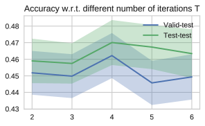
Figure 1: Mean accuracy scores with 95% confidence intervals, computed on episodes from $\omathcal{D}_{\operatorname{test}}$, of various methods on 1-shot and 5-shot classification problems on MiniImagenet.

Figure 2: Meta-validation of the number
of gradient descent steps on ground models
parameters $T$ for one-shot learning.

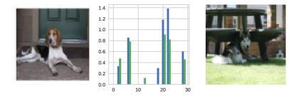
Figure 3: After sampling two datasets $D\in\omathcal{D}_{\rm tr}$ and $D^{\prime}\in\omathcal{D^{\prime}}_{\rm test}$, we show on the left the two images $x\in D,\;x^{\prime}\in D$ that minimize $||h(x,\lambda)-h(x^{\prime},\lambda)||$ and on the right the ones that maximize it. In between each of the two couples we compare a random subset of components of $h(x,\lambda)$ (blue) and $h(x^{\prime},\lambda)$ (green).

Ongoing experiments aim at combining the first and the second design patterns outlined in Section 4 both in depth (lower layers weights are hyperparameters and higher layers weights initial points) and in width (a portion of filters constitutes the meta-representation, while the weights relative to the rest of filters are considered initialization), and at experimenting with the third pattern. Moreover we plan to explore settings in which different datasets come form various domains (e.g. visual, natural language, speech, etc.), are linked to diverse tasks (e.g. classification, localization, segmentation, generation and others) and have structurally different instance spaces.

5 Conclusions

We observed that hyperparameter optimization and learning-to-learn share the same mathematical structure, captured by a bilevel programming problem, which consists in minimizing an outer objective function whose value implicitly depends on the solution of an inner problem. The objective function of this latter problem — whose optimization variables are identified with the parameters of (ground) models — is, in turn, parametrized by the outer problem variables, identified either as hyperparameters or parameters of a meta-model, depending on the context. Since the solution of the inner optimization problem does not have, in general, a closed form expression, we formulate a related constrained optimization problem by considering explicitly an optimization dynamics for the inner problem (e.g. gradient descent). In this way we are able to (A) compute the outer objective and optimize it by gradient descent and (B) optimize also variables that parametrize the learning dynamics. We discussed examples of the framework and present experiments on few-shots learning, introducing a method for learning a shared, cross-episode, representation.

Appendix A On variants of representation learning methods

We report in Table 1 additional results on a series of experiments for one-shot learning on MiniImagenet with the aim of comparing out method for learning a meta-representation outlined in Sections 3 and 4 with other methods for learning representations that involve the factorization of a classifier as $g^{j}\circ h$. The representation mapping $h$ is either pretrained on the classification problem with all the images in the training meta-dataset or learned with different meta-learning algorithms. In all the experiments, for each episode $g^{j}$ is a multinomial logistic regressor learned with few iterations of gradient descent as described in Section 4.

Method	Accuracy 1-shot	Method	Accuracy 1-shot
NN-conv	$39.97$	Bilevel-train 1x5	$27.36$
NN-linear	$41.50$	Bilevel-train 16x5	$29.63$
NN-softmax	$41.36$	Approx-train 1x5	$24.74$
Multiclass-conv	$36.57$	Approx-train 16x5	$38.80$
Multiclass-linear	$43.02$	Classic-train 1x5	$24.70$
Multiclass-softmax	$37.60$	Classic-train 16x5	$40.46$

Table 1: Performance of various methods where the representation is either transfered from models trained in a standard multiclass supervised learning setting (left column) or learned in a meta-learning setting (left column).

In the experiments in the left column we use as representation mapping $h$ the outputs of different layers of two distinct neural networks (denominated NN and Multiclass in the Table) trained with a standard multiclass supervised learning approach on the totality of examples contained in the training meta-dataset (600 examples for each of the 64 classes ). The first network NN, which has 64 filters per layer, achieves a test accuracy of $43.41\%$. It is the same network used to reproduce the Nearest-neighbour baseline in Table 2 and it has been trained with an early stopping procedure on the nearest-neighbour classification accuracy computed on episodes sampled from the validation meta-dataset. The network Multiclass, which has 32 filters per layer, has instead been trained with an early stopping procedure on the accuracy on a small held-out validation set. Achieving a test accuracy of $46.33$, this second model is superior on the (standard) multiclass classification problem. For each of the network we report experiment using as representation different layers. Specifically:

• conv: we use the output of the last convolutional layer as representation, that is $h(x)\in\mathbb{R}^{2304}_{+}$ for NN and $h(x)\in\mathbb{R}^{1152}_{+}$ for Multiclass;

• linear: we use as representation the linear output layer (before applying the softmax operation), so that $h(x)\in\mathbb{R}^{64}$.

• softmax: the representation is given by the probability distribution output of the network; in this case $h(x)\in(0,1)^{64}$

The linear representation yields the best result for both of the networks and in the case of Multiclass achieves comparable results with previously proposed meta-learning methods.

The experiments in the right column, where $h$ is learned with meta-learning techniques, span in two directions: the first one is that of verifying the impact of various approximations on the computation of the hypergradient, and the second one is to empirically assess the importance of the training/validation splitting of each training episode. In the experiments denoted Bilevel-train, we use a bilevel approach but, unlike in section 4, we optimize the parameter vector $\lambda$ of the representation mapping by minimizing the loss on the training sets. The outer objective is thus given by

$$f(\lambda)=\sum\limits_{j=1}^{N}\frac{1}{|D^{j}_{\operatorname{tr}}|}\sum\limits_{z\in D^{j}_{\operatorname{tr}}}E^{j}(w^{j}_{T},\lambda,z).$$

We consider episodes with training set composed by 1 and 16 examples per class, denoted (1x5) and (16x5) respectively. In these cases $f(\lambda)$ goes quickly to 0 and the learning ceases after few hundred iterations. In Approx experiments we consider an approximation of the hypergradient $\nabla f(\lambda)$ by disregarding the optimization dynamics of the inner objectives (i.e. we set $\partial_{\lambda}w^{j}_{T}=0$). We also run this experiment considering the training/validation splitting obtaining a final test accuracy of $41.12\%$. In the experiments denoted as Classic we jointly minimize

$$f(\lambda,w^{1},\dots,w^{N})=\sum\limits_{j=1}^{N}\frac{1}{|D^{j}_{\operatorname{tr}}|}\sum\limits_{z\in D^{j}_{\operatorname{tr}}}E^{j}(w^{j},\lambda,z).$$

and treat the problem as a standard multitask learning problem as suggested in (Baxter,, 1995) (with the exception that we evaluate $f$ a mini-batches of 4 episodes, randomly sampled every 4 gradient descent iterations).

This series of experiments suggest that both the training/validation splitting and the full computation of the hypergradient constitute key factors for learning a good meta-representation. Nevertheless, provided that the training sets contain a sufficient number of examples, also the joint optimization method achieves decent results, while learning the representation using only the training sets of one-shot episodes (experiments train 1x5) proves unsuccessful in every tested setting, a result in line with the theoretical analysis in (Baxter,, 1995). On the other side, using pretrained representations, specially in a low-dimensional space, turns out to be a rather effective baseline. One possible explanation is that, in this context, some classes in the training and testing meta-datasets are rather similar (e.g. various dog breeds) and thus ground classifiers can leverage on very specific representations.

References

- Andrychowicz et al., (2016) Andrychowicz, M., Denil, M., Gomez, S., Hoffman, M. W., Pfau, D., Schaul, T., and de Freitas, N. (2016). Learning to learn by gradient descent by gradient descent. In Advances in Neural Information Processing Systems, pages 3981–3989.
- Baxter, (1995) Baxter, J. (1995). Learning internal representations. In Proceedings of the eighth annual conference on Computational learning theory, pages 311–320. ACM.
- Baxter, (1998) Baxter, J. (1998). Theoretical models of learning to learn. Learning to learn, pages 71–94.
- Bengio et al., (2009) Bengio, Y. et al. (2009). Learning deep architectures for ai. Foundations and trends® in Machine Learning, 2(1):1–127.
- Bergstra and Bengio, (2012) Bergstra, J. and Bengio, Y. (2012). Random search for hyper-parameter optimization. Journal of Machine Learning Research, 13(Feb):281–305.
- Bergstra et al., (2013) Bergstra, J., Yamins, D., and Cox, D. D. (2013). Making a Science of Model Search: Hyperparameter Optimization in Hundreds of Dimensions for Vision Architectures. ICML (1), 28:115–123.
- Bergstra et al., (2011) Bergstra, J. S., Bardenet, R., Bengio, Y., and Kégl, B. (2011). Algorithms for hyper-parameter optimization. In Advances in Neural Information Processing Systems, pages 2546–2554.
- Colson et al., (2007) Colson, B., Marcotte, P., and Savard, G. (2007). An overview of bilevel optimization. Annals of operations research, 153(1):235–256.
- Deng et al., (2009) Deng, J., Dong, W., Socher, R., Li, L.-J., Li, K., and Fei-Fei, L. (2009). Imagenet: A large-scale hierarchical image database. In Computer Vision and Pattern Recognition, 2009. CVPR 2009. IEEE Conference on, pages 248–255. IEEE.
- Domke, (2012) Domke, J. (2012). Generic Methods for Optimization-Based Modeling. In AISTATS, volume 22, pages 318–326.
- Finn et al., (2017) Finn, C., Abbeel, P., and Levine, S. (2017). Model-agnostic meta-learning for fast adaptation of deep networks. In Proceedings of the 34th International Conference on Machine Learning, ICML 2017, pages 1126–1135.
- Franceschi et al., (2017) Franceschi, L., Donini, M., Frasconi, P., and Pontil, M. (2017). Forward and reverse gradient-based hyperparameter optimization. In Proceedings of the 34th International Conference on Machine Learning, ICML 2017, pages 1165–1173.
- Goodfellow et al., (2016) Goodfellow, I., Bengio, Y., and Courville, A. (2016). Deep Learning. MIT Press.
- Griewank and Walther, (2008) Griewank, A. and Walther, A. (2008). Evaluating derivatives: principles and techniques of algorithmic differentiation. SIAM.
- Hutter et al., (2015) Hutter, F., Lücke, J., and Schmidt-Thieme, L. (2015). Beyond Manual Tuning of Hyperparameters. KI - Künstliche Intelligenz, 29(4):329–337.
- Maclaurin et al., (2015) Maclaurin, D., Duvenaud, D., and Adams, R. P. (2015). Gradient-based hyperparameter optimization through reversible learning. In Proceedings of the 32nd International Conference on Machine Learning.
- Maurer, (2005) Maurer, A. (2005). Algorithmic stability and meta-learning. Journal of Machine Learning Research, 6:967–994.
- Maurer et al., (2016) Maurer, A., Pontil, M., and Romera-Paredes, B. (2016). The benefit of multitask representation learning. Journal of Machine Learning Research, 17(81):1–32.
- Mishra et al., (2017) Mishra, N., Rohaninejad, M., Chen, X., and Abbeel, P. (2017). Meta-Learning with Temporal Convolutions. arXiv:1707.03141 [cs, stat].
- Moore et al., (2011) Moore, G., Bergeron, C., and Bennett, K. P. (2011). Model selection for primal SVM. Machine Learning, 85(1-2):175–208.
- Pedregosa, (2016) Pedregosa, F. (2016). Hyperparameter optimization with approximate gradient. In Proceedings of The 33rd International Conference on Machine Learning, volume 48 of Proceedings of Machine Learning Research, pages 737–746. PMLR.
- Ravi and Larochelle, (2017) Ravi, S. and Larochelle, H. (2017). Optimization as a model for few-shot learning. ICLR.
- Santoro et al., (2016) Santoro, A., Bartunov, S., Botvinick, M., Wierstra, D., and Lillicrap, T. (2016). Meta-learning with memory-augmented neural networks. In International conference on machine learning, pages 1842–1850.
- Thrun and Pratt, (1998) Thrun, S. and Pratt, L. (1998). Learning to learn. Springer.
- Vinyals et al., (2016) Vinyals, O., Blundell, C., Lillicrap, T., Kavukcuoglu, K., and Wierstra, D. (2016). Matching networks for one shot learning. In Advances in Neural Information Processing Systems 29: Annual Conference on Neural Information Processing Systems 2016, pages 3630–3638.
- Wichrowska et al., (2017) Wichrowska, O., Maheswaranathan, N., Hoffman, M. W., Colmenarejo, S. G., Denil, M., de Freitas, N., and Sohl-Dickstein, J. (2017). Learned optimizers that scale and generalize. In Proceedings of the 34th International Conference on Machine Learning, ICML 2017, Sydney, NSW, Australia, 6-11 August 2017, pages 3751–3760.