Possible $\eta^{\prime}d$ bound state and its $s$-channel formation in the $\gamma d\to\eta d$ reaction

Abstract

We theoretically investigate a possibility of an $\eta^{\prime}d$ bound state and its formation in the $\gamma d\to\eta d$ reaction. First, in the fixed center approximation to the Faddeev equations we obtain an $\eta^{\prime}d$ bound state with a binding energy of $25\text{ MeV}$ and width of $19\text{ MeV}$, where we take the $\eta^{\prime}N$ interaction with a coupling to the $\eta N$ channel from the linear $\sigma$ model. Then, in order to investigate the feasibility from an experimental point of view, we calculate the cross section of the $\gamma d\to\eta d$ reaction at the photon energy in the laboratory frame around $1.2\text{ GeV}$. As a result, we find a clear peak structure with the strength $\sim 0.2\text{ nb}/\text{sr}$, corresponding to a signal of the $\eta^{\prime}d$ bound state in case of backward $\eta$ emission. This structure will be prominent because a background contribution coming from single-step $\eta$ emission off a bound nucleon is highly suppressed. In addition, the signal can be seen even in case of forward $\eta$ emission as a bump or dip, depending on the relative phase between the bound-state formation and the single-step background.

I Introduction

The properties of hadrons are of great interest to understand the nonperturbative behavior of the fundamental theory of strong interactions, quantum chromodynamics (QCD). Dynamical quark-mass generation is a subject to be studied, where chiral symmetry plays a key role. An order parameter of the spontaneous breakdown of chiral symmetry in the QCD vacuum is the chiral condensate. The masses of the light vector mesons ($\rho$, $\omega$, and $\phi$) are considered to be mostly induced by this order parameter. In this regard, mass modifications of the vector mesons at finite density and/or finite temperature have been studied both theoretically and experimentally Metag:2017yuh . No clear evidence for them has been observed so far. Another candidate to study the relationship between the mass and chiral condensate is the $\eta^{\prime}(958)$ meson. It has an exceptionally large mass although it would be a Nambu-Goldstone boson originating from the $\text{U}_{\rm L}(3)\times\text{U}_{\rm R}(3)$ chiral symmetry breaking Weinberg:1975ui . Its mass generation is considered to be a result of the quantum anomaly in QCD which breaks $\text{U}_{\rm A}(1)$ symmetry tHooft:1976rip ; Witten:1979vv ; Veneziano:1979ec . In addition, it was also pointed out that the chiral condensate plays an essential role for the anomaly to affect the $\eta^{\prime}$ mass Cohen:1996ng ; Lee:1996zy .

In this line, various studies on the in-medium properties of the $\eta^{\prime}$ meson are performed to understand QCD in the nuclear medium theoretically Jido:2011pq ; Pisarski:1983ms ; Bernard:1987sg ; Kunihiro:1989my ; Kapusta:1995ww ; Tsushima:1998qp ; Costa:2002gk ; Nagahiro:2004qz ; Bass:2005hn ; Nagahiro:2006dr ; Nagahiro:2011fi ; Sakai:2013nba ; Bass:2013nya and experimentally Nanova:2012vw ; Nanova:2013fxl ; Nanova:2016cyn ; Tanaka:2016bcp . In particular, from the theoretical side, assuming the mass difference between $\eta^{\prime}$ and low-lying pseudoscalar mesons comes from the chiral condensate in connection with the $\text{U}_{\rm A}(1)$ anomaly, we expect that the $\eta^{\prime}$ mass will be reduced by an order of 100 MeV at normal nuclear density, because partial restoration of chiral symmetry in a nuclear medium, which was suggested by pionic atoms as a reduction of the chiral order parameter Suzuki:2002ae , induces suppression of the $\text{U}_{\rm A}(1)$ anomaly effect to the $\eta^{\prime}$ mass Jido:2011pq . A chiral effective model calculation by the linear $\sigma$ model implies a $\eta^{\prime}$ mass reduction of $\sim 80\text{ MeV}$ at normal nuclear density Sakai:2013nba . A more sophisticated calculation based on the Nambu–Jona-Lasinio model, in which the $\text{U}_{\rm A}(1)$ effect is introduced by the Kobayashi-Maskawa-’t Hooft term, predicts a large reduction of approximately 150 MeV at normal nuclear density Costa:2002gk . Such a large reduction of the $\eta^{\prime}$ mass allows formation of $\eta^{\prime}$-nucleus bound states ($\eta^{\prime}$-mesic nuclei). From the experimental side, the results obtained by the CBELSA/TAPS collaboration imply an attractive and weakly absorptive potential Metag:2017yuh ; Nanova:2012vw ; Nanova:2013fxl ; Nanova:2016cyn : the real part of the $\eta^{\prime}$-nucleus potential at normal nuclear density was found to be $-37\pm 10(\text{stat})\pm 10(\text{syst})\text{ MeV}$ in the $\eta^{\prime}$ photoproduction from ${}^{12}\text{C}$ Nanova:2013fxl and $-41\pm 10(\text{stat})\pm 15(\text{syst})\text{ MeV}$ from ${}^{93}\text{Nb}$ Nanova:2016cyn , while its imaginary part was found to be $-(10\pm 2.5)\text{ MeV}$ Nanova:2012vw . At GSI, the excitation spectrum for the ${}^{12}{\rm C}(p,d)$ reaction was measured to search for $\eta^{\prime}$-mesic nuclei Tanaka:2016bcp . The result of the GSI experiment seems to exclude strongly attractive $\eta^{\prime}$-nucleus potential with a mass reduction of $\gtrsim 150\text{ MeV}$ at normal nuclear density, but is still consistent with the $\eta^{\prime}$ mass reduction of $\lesssim 80\text{ MeV}$. To pin down the properties of the $\eta^{\prime}$ meson in nuclei more rigorously, we need various experimental information on $\eta^{\prime}$-nucleon and $\eta^{\prime}$-nucleus systems, such as the $\eta^{\prime}N$ scattering length in free space Czerwinski:2014yot .

We here emphasize that the $\eta^{\prime}$ mass reduction in a nuclear medium is induced by an attractive $\eta^{\prime}N$ interaction. In this sense, the $\eta^{\prime}N$ interaction plays a key role to investigate properties of the $\eta^{\prime}$ meson. Because experimental information on the $\eta^{\prime}N$ interaction is not sufficient, we employ symmetry properties of hadrons to deduce the $\eta^{\prime}N$ interaction. The $\eta^{\prime}N$ interaction was studied in, e.g., the chiral effective model Kawarabayashi:1980uh ; Bass:1999is ; Borasoy:1999nd ; Oset:2010ub ; Sakai:2013nba . In terms of the linear $\sigma$ model, the scalar meson exchange provides an attractive interaction between $\eta^{\prime}$ and nucleon which is strong enough to bind the $\eta^{\prime}N$ system Sakai:2013nba . Experimentally, the existence of an $\eta^{\prime}N$ bound state is implied by near-threshold behavior of the total cross section of the $\pi^{-}p\to\eta^{\prime}n$ reaction Moyssides:1983 . It has been also pointed out that $\eta^{\prime}n$ bound state, if exists, can be observed in incoherent photoproduction off a deuteron target $\gamma d\to\eta np$ Sekihara:2016jgx .

In this study we extend the consideration on the $\eta^{\prime}N$ system to the $\eta^{\prime}d$ system. We take the $\eta^{\prime}N$ interaction from the linear $\sigma$ model Sakai:2013nba and solve the Faddeev equation for the $\eta^{\prime}d$ system in a certain approximation. We will see that the $\eta^{\prime}d$ system is bound thanks to a strongly attractive $\eta^{\prime}N$ interaction in our model. We further discuss whether this $\eta^{\prime}d$ bound state can be observed in experiments or not. For this purpose we choose the $\gamma d\to\eta d$ reaction, in which the $\eta^{\prime}d$ bound state can be formed in the $s$-channel process and decays into $\eta d$. The biggest advantage of this reaction is that we can easily perform the center-of-mass energy scan to search for the $\eta^{\prime}d$ bound state by varying the photon energy. Because the $\eta^{\prime}d$ threshold is $2.833\text{ GeV}$, the photon energy appropriate for the bound-state search is around $1.20\text{ GeV}$ in the laboratory frame. In addition, it is worth mentioning that the final-state $\eta d$ can specify an isospin $0$ state in its $s$ channel. In the following we will formulate the $\gamma d\to\eta d$ reaction mechanism and calculate its cross section to estimate the production cross section of the $\eta^{\prime}d$ bound state.

This paper is organized as follows. In Sec. II we show that the $\eta^{\prime}N$ interaction from the linear $\sigma$ model leads to an $\eta^{\prime}d$ bound state. Next, in Sec. III we evaluate the cross section of the $\gamma d\to\eta d$ reaction, in which an $\eta^{\prime}d$ bound state may be generated, by using phenomenological $\gamma N\to\eta^{(\prime)}N$ amplitudes and the $\eta^{\prime}N$ interaction constructed in the linear $\sigma$ model. Section IV is devoted to the summary of this paper. Throughout this study we assume isospin symmetry for hadron masses as well as strong interactions.

II Possible $\eta^{\prime}d$ bound state

II.1 $\eta^{\prime}N$ system

Figure 1: Diagrammatic equation for the $\eta^{(\prime)}N\to\eta^{(\prime)}N$ scattering amplitude. The solid and dashed lines represent the nucleon and $\eta^{(\prime)}$, respectively. The shaded squares and dots are the full scattering amplitude and tree-level interaction, respectively.

First of all, we consider the $\eta^{\prime}N$ interaction. We focus on the $s$-wave $\eta^{\prime}N$ system, and take into account a coupling to the $\eta N$ channel because it is the closest open channel coupled in the $s$ wave. We employ the $\eta^{\prime}N$ interaction in the linear $\sigma$ model with the unitarization according to Ref. Sakai:2013nba . Dynamics in the $\eta^{\prime}p$ and $\eta^{\prime}n$ systems is the same, because we assume isospin symmetry. We assign a channel index of $1$ ($2$) to the $\eta^{\prime}N$ ($\eta N$) channel. In the linear $\sigma$ model, the $\eta^{\prime}N$ interaction can be described by the exchange of the singlet and octet $\sigma$ mesons. In momentum space, the interaction $V_{jk}$ with the channel indices $j$ and $k$ can be written as Sakai:2013nba

$$V_{11}=-\frac{6gB}{\sqrt{3}m_{\sigma_{0}}^{2}},\quad V_{12}=V_{21}=+\frac{6gB}{\sqrt{6}m_{\sigma_{8}}^{2}},\quad V_{22}=0,$$ (1)

where the constants $g$, $B$, $m_{\sigma_{0}}$, and $m_{\sigma_{8}}$ determine the strength of the interaction; $g$ is the $\sigma NN$ coupling constant, $B$ is the contribution from the $\text{U}_{\rm A}(1)$ anomaly, and $m_{\sigma_{0}}$ and $m_{\sigma_{8}}$ are the masses of the singlet and octet $\sigma$ mesons.

It should be noted that the interaction in Eq. (1) is the leading-order term of the momentum expansion in the flavor SU(3) symmetric limit. When we switch on the flavor symmetry breaking by the heavier strange quark than up and down quarks, the $\eta$-$\eta^{\prime}$ mixing angle is $-6.2$ degrees in the linear $\sigma$ model Sakai:2013nba . Even in this case of the linear $\sigma$ model, the modification of the $\eta^{\prime}N$ interaction by the $\eta$-$\eta^{\prime}$ mixing is small Sakai:2013nba , owing to the dominance of the singlet $\eta$ in the physical $\eta^{\prime}$ state. Furthermore, the strength of the $\eta^{\prime}N\to\eta^{\prime}N$ part, which is crucial in the following discussions, shifts only several percent for the $\eta$-$\eta^{\prime}$ mixing angle between $0$ and $-20$ degrees, which is adopted in Ref. Bass:2013nya .

Then the $\eta^{\prime}N$ scattering amplitude $T_{jk}(w)$, as a function of the energy of the $\eta^{\prime}N$ system $w$, is a solution of the Lippmann–Schwinger equation diagrammatically expressed in Fig. 1. This equation can be written in the present formulation as

$$T_{jk}(w)=V_{jk}+\sum_{l=1}^{2}V_{jl}G_{l}(w)T_{lk}(w)$$ (2)

with the $\eta^{(\prime)}N$ loop function $G_{j}$. Because the interaction $V_{jk}$ is independent of the external momentum as in Eq. (1), the scattering equation (2) becomes algebraic. For the $\eta^{(\prime)}N$ loop function, we employ a covariant expression as

$$G_{j}(w)\equiv i\int\frac{d^{4}q}{(2\pi)^{4}}\frac{2m_{N}}{[(p-q)^{2}-m_{N}^{2}+i0](q^{2}-m_{j}^{2}+i0)}$$ (3)

with $p^{\mu}=(w,\,\bm{0})$, the nucleon mass $m_{N}$, and $m_{1}=m_{\eta^{\prime}}$ and $m_{2}=m_{\eta}$ being the $\eta^{\prime}$ and $\eta$ masses, respectively. The loop function is calculated with the dimensional regularization as

$$G_{j}(w)=\frac{2m_{N}}{16\pi^{2}}\Bigg{[}a_{j}(\mu_{\rm reg})+\ln\left(\frac{m_{N}^{2}}{\mu_{\rm reg}^{2}}\right)$$

$$+\frac{w^{2}+m_{j}^{2}-m_{N}^{2}}{2w^{2}}\ln\left(\frac{m_{j}^{2}}{m_{N}^{2}}\right)$$

$$-\frac{\lambda^{1/2}(w^{2},\,m_{N}^{2},\,m_{j}^{2})}{w^{2}}\text{arctanh}\left(\frac{\lambda^{1/2}(w^{2},\,m_{N}^{2},\,m_{j}^{2})}{m_{N}^{2}+m_{j}^{2}-w^{2}}\right)\Bigg{]}$$ (4)

with the regularization scale $\mu_{\rm reg}$, the subtraction constant $a_{j}$, and $\lambda(x,\,y,\,z)\equiv x^{2}+y^{2}+z^{2}-2xy-2yz-2zx$. In this study the subtraction constant is fixed by the natural renormalization scheme developed in Ref. Hyodo:2008xr so as to exclude the Castillejo-Dalitz-Dyson pole contribution from the loop function. This can be achieved by requiring $G_{j}(w=m_{N})=0$ for every channel $j$, which results in $a_{1}(\mu_{\rm reg}=m_{N})=-1.84$ and $a_{2}(\mu_{\rm reg}=m_{N})=-1.24$ in the present construction.

Now we fix the model parameters as in Ref. Sakai:2013nba , i.e., $g=7.67$, $B=0.984\text{ GeV}$, $m_{\sigma_{0}}=0.7\text{ GeV}$, and $m_{\sigma_{8}}=1.23\text{ GeV}$, with which we obtain an $\eta^{\prime}N$ bound state. The pole position of the $\eta^{\prime}N$ bound state is $1889-6i\text{ MeV}$, which corresponds to the binding energy of $8\text{ MeV}$ measured from the $\eta^{\prime}N$ threshold and decay width of $12\text{ MeV}$. The existence of an $\eta^{\prime}N$ bound state is implied by near-threshold behavior of the total cross section of the $\pi^{-}p\to\eta^{\prime}n$ reaction Moyssides:1983 , although no bump corresponding to the $\eta^{\prime}n$ bound state has been observed in the $\gamma d\to pX$ reaction at LEPS Muramatsu . In the $\eta^{\prime}N$ scattering, the contribution from the $\eta N$ channel is found to be small while the elastic $\eta^{\prime}N$ interaction is dominant. This is because the transition of the $\eta^{\prime}N$ channel to the $\eta N$ channel is suppressed by the larger mass of the octet scalar meson.

II.2 $\eta^{\prime}d$ system

Next, using the $\eta^{\prime}N$ interaction constructed in the previous subsection, we formulate the $\eta^{\prime}d$ scattering amplitude. We treat the $\eta^{\prime}pn$ three-body system, where we consider the $pn$ subsystem as a deuteron and solve the Faddeev equation in the so-called fixed center approximation (FCA) Bayar:2011qj ; Sekihara:2016vyd . We incorporate two channels for the three-body system: 1) $\eta^{\prime}pn$ and 2) $pn\eta^{\prime}$. We distinguish either $\eta^{\prime}$ appears in the left or right, according to the formulation in Ref. Sekihara:2016vyd . For instance, if the initial state is $\eta^{\prime}pn$ ($pn\eta^{\prime}$), the multiple scattering starts with the $\eta^{\prime}p$ ($\eta^{\prime}n$) scattering in the system. Similarly, if the final state is $\eta^{\prime}pn$ ($pn\eta^{\prime}$), the multiple scattering ends with the $\eta^{\prime}p$ ($\eta^{\prime}n$) scattering in the system. Besides, we can fix the ordering of the nucleons, $pn$, without loss of generality. In the three-body problem, the $\eta$ meson does not appear explicitly but is intrinsically treated in the two-body $\eta^{\prime}N\to\eta^{\prime}N$ amplitude.

Figure 2: Diagrammatic equation for the multiple $\eta^{\prime}$ scattering amplitude of the process $\eta^{\prime}pn\to\eta^{\prime}pn$. The small shaded boxes represent the $\eta^{\prime}N\to\eta^{\prime}N$ scattering amplitude, and the large open boxes indicate its multiple scattering amplitude.

In order to grasp the construction, we first consider the $\eta^{\prime}pn\to\eta^{\prime}pn$, i.e., channel $1\to 1$ scattering amplitude $T_{11}^{\rm FCA}$. This is schematically expressed in Fig. 2 as a diagrammatic equation and can be written as

$$T^{\rm FCA}_{11}(W)= t_{1}(W)+t_{1}(W)G_{\eta^{\prime}}^{\rm FCA}(W)T^{\rm FCA}_{21}(W)$$ (5)

with the total three-body energy $W$ and the three-body Green function $G_{\eta^{\prime}}^{\rm FCA}$ of the $\eta^{\prime}$ propagation. The two-body $\eta^{\prime}N\to\eta^{\prime}N$ scattering amplitude $t_{1}$ is developed in the previous subsection

$$t_{1}(W)=T_{11}(w^{\rm FCA}(W))$$ (6)

with the $\eta^{\prime}N$ two-body center-of-mass energy $w^{\rm FCA}$. We evaluate the two-body energy $w^{\rm FCA}$ as a function of the three-body energy $W$ Bayar:2011qj ; Sekihara:2016vyd by treating two nucleons as one particle of mass $2m_{N}$:

$$w^{\rm FCA}(W)=\sqrt{\frac{W^{2}+m_{\eta^{\prime}}^{2}-2m_{N}^{2}}{2}}.$$ (7)

The three-body Green function $G_{\eta^{\prime}}^{\rm FCA}$ is defined as:

$$G_{\eta^{\prime}}^{\rm FCA}(W)=\int\frac{d^{3}p}{(2\pi)^{3}}\frac{F_{NN}(p)}{p_{\eta^{\prime}}^{0}(W)^{2}-\bm{p}^{2}-m_{\eta^{\prime}}^{2}+i0}$$ (8)

with the $\eta^{\prime}$ energy $p_{\eta^{\prime}}^{0}$

$$p_{\eta^{\prime}}^{0}(W)=\frac{W^{2}+m_{\eta^{\prime}}^{2}-(2m_{N})^{2}}{2W},$$ (9)

and the deuteron form factor $F_{NN}(p)$

$$F_{NN}(p)=\int d^{3}re^{i\bm{p}\cdot\bm{r}}|\varphi(r)|^{2}.$$ (10)

Here $\varphi(r)$ is the deuteron wave function in coordinate space, and the form factor can be rewritten as

$$F_{NN}(p)=\int\frac{d^{3}q}{(2\pi)^{3}}\tilde{\varphi}(q)\tilde{\varphi}(|\bm{q}-\bm{p}|)$$ (11)

with the deuteron wave function in momentum space $\tilde{\varphi}(q)$. For the deuteron wave function, we neglect the $d$-wave component and use a parameterization of the $s$-wave component given in an analytic function Lacombe:1981eg as

$$\tilde{\varphi}(q)=\sum_{j=1}^{11}\frac{C_{j}}{q^{2}+m_{j}^{2}}$$ (12)

with $C_{j}$ and $m_{j}$ determined with the charge-dependent Bonn potential Machleidt:2000ge . This wave function is normalized so as to satisfy $F_{NN}(p=0)=1$.

Figure 3: Absolute value of the scattering amplitude $T_{11}^{\rm FCA}+T_{12}^{\rm FCA}$ as a function of the total three-body energy $W$. The vertical dotted line indicates the $\eta^{\prime}NN$ threshold.

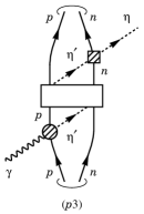
Figure 4: Diagrams for the $\gamma d\to\eta d$ reaction. The shaded circles represent the $\gamma N\to\eta^{(\prime)}N$ amplitude. The small shaded boxes indicate the $\eta^{\prime}N\to\eta N$ amplitude. The large open boxes represent the multiple scattering amplitude for the $\eta^{\prime}pn$ system.

The scattering equation (5) can be straightforwardly extended to the two-channel case, and we obtain

$$T^{\rm FCA}_{ab}(W)=V_{ab}^{\rm FCA}(W)$$

$$\quad+\sum_{c=1}^{2}\tilde{V}_{ac}^{\rm FCA}(W)G_{c}^{\rm FCA}(W)T^{\rm FCA}_{cb}(W).$$ (13)

Here $a$, $b$, and $c$ ($=1$, $2$) are three-body channel indices and $V_{ab}^{\rm FCA}$ and $\tilde{V}_{ab}^{\rm FCA}$ contain the $\eta^{\prime}N\to\eta^{\prime}N$ scattering amplitude as follows:

$$V_{ab}^{\rm FCA}=\left(\begin{array}[]{@{\,}cc@{\,}}t_{1}&0\\ 0&t_{1}\\ \end{array}\right),\quad\tilde{V}_{ab}^{\rm FCA}=\left(\begin{array}[]{@{\,}cc@{\,}}0&t_{1}\\ t_{1}&0\\ \end{array}\right).$$ (14)

The three-body loop function $G_{a}^{\rm FCA}$ is

$$G_{1}^{\rm FCA}=G_{2}^{\rm FCA}=G_{\eta^{\prime}}^{\rm FCA}.$$ (15)

With this formulation, we can calculate the $\eta^{\prime}d$ scattering amplitude as a function of the total three-body energy $W$.

As we will see later, the multiple scattering amplitude practically appears as the sum of the $\eta^{\prime}pn$ and $pn\eta^{\prime}$ contributions, such as $T_{11}^{\rm FCA}+T_{12}^{\rm FCA}$, in full reaction amplitudes. The absolute value of this scattering amplitude $T_{11}^{\rm FCA}+T_{12}^{\rm FCA}$ is shown in Fig. 3 as a function of the total three-body energy $W$. As one can see, the amplitude has a peak structure corresponding to the $\eta^{\prime}d$ bound state. In the amplitude we find the pole of the $\eta^{\prime}d$ bound state at $2809-10i\text{ MeV}$ in the complex energy plane, which corresponds to the binding energy $25\text{ MeV}$ measured from the $\eta^{\prime}d$ threshold and width $19\text{ MeV}$. The binding energy increases more than twice compared to the $\eta^{\prime}N$ bound state because the number of the potential terms increases more than that of the kinetic energy, as in usual many-body systems.

III $s$-channel formation of the $\eta^{\prime}d$ bound state in the $\gamma d\to\eta d$ reaction

Because the $\eta^{\prime}d$ system is bound with the $\eta^{\prime}N$ interaction deduced from the linear $\sigma$ model, it may be experimentally generated in certain reactions. In this section, we consider the $\gamma d\to\eta d$ reaction and examine a possibility of observing its signal. We first formulate the $\gamma d\to\eta d$ scattering amplitude in Sec. III.1, and show the numerical results in Sec. III.2.

III.1 Formulation

In order to calculate the scattering amplitude of the $\gamma d\to\eta d$ reaction, we introduce six diagrams relevant to the formation of the $\eta^{\prime}d$ bound state as shown in Fig. 4:

$$T_{\gamma d\to\eta d}= \mathcal{T}_{p1}+\mathcal{T}_{p2}+\mathcal{T}_{p3}+\mathcal{T}_{n1}+\mathcal{T}_{n2}+\mathcal{T}_{n3}.$$ (16)

On the one hand, $\mathcal{T}_{p1}$ and $\mathcal{T}_{n1}$ are the single-step scatterings for the reaction, which becomes a background in view of the signal of the $\eta^{\prime}d$ bound-state formation. On the other hand, the remaining four terms contain the multiple $\eta^{\prime}$ scattering on both $p$ and $n$ which generates the $\eta^{\prime}d$ bound state. We here neglect diagrams in which the $\eta$ meson is produced in the intermediate state, because around the $\eta^{\prime}d$ threshold the $\eta$ meson in the intermediate state should go highly off-shell and should be kinematically suppressed. This resembles the case of photoproduction of the $\eta^{\prime}n$ bound state in the $\gamma d\to\eta np$ reaction, as discussed in Ref. Sekihara:2016jgx . The reaction diagrams in Fig. 4 contain the $\gamma N\to\eta N$ and $\gamma N\to\eta^{\prime}N$ scattering amplitudes and the transition amplitude of the $\eta^{\prime}d$ bound state to the final-state $\eta d$ system.

Below, we formulate the $\gamma N\to\eta N$ and $\gamma N\to\eta^{\prime}N$ scattering amplitudes based on the experimental data. We then construct the $\gamma d\to\eta d$ scattering amplitude (16) from the amplitudes of $\gamma N\to\eta^{(\prime)}N$, multiple $\eta^{\prime}$ scattering on $pn$, and transition to $\eta d$. In the present formulation of the $\gamma d\to\eta d$ amplitude, we will fix the photo-induced $\gamma N\to\eta^{(\prime)}N$ amplitudes so as to reproduce the existing experimental data of $\eta^{(\prime)}$ photoproduction. Therefore, when we modify the $\eta^{\prime}N$ interaction, they affect only the amplitudes of the multiple $\eta^{\prime}$ scattering on $pn$ and of $\eta^{\prime}N\to\eta N$ entering in the $\eta^{\prime}d\to\eta d$ transition in our model.

III.1.1 $\gamma N\to\eta N$ and $\gamma N\to\eta^{\prime}N$ scattering amplitudes

Let us consider the $\gamma p\to\eta p$ and $\gamma n\to\eta n$ scattering amplitudes. For these reactions, there exist various experimental data of the differential cross sections as a function of the photon energy in the laboratory frame $E_{\gamma}^{\rm lab}$ and the $\eta$ scattering angle in the center-of-mass frame $\theta_{\eta}$, around the photon energy of interest, $E_{\gamma}^{\rm lab}\approx 1.2\text{ GeV}$: for instance, the free proton target case Nakabayashi:2006ut ; Bartholomy:2007zz ; Williams:2009yj ; Sumihama:2009gf ; Crede:2009zzb ; McNicoll:2010qk and the deuteron target case Jaegle:2011sw ; Werthmuller:2014thb ; Ishikawa:2016rgk ; Witthauer:2017pcy . Several theoretical analyses of these data are available as well, e.g., in Refs. Chiang:2002vq ; Anisovich:2011fc ; Kamano:2013iva ; Ronchen:2015vfa .

For the $\gamma p\to\eta p$ reaction, we take the theoretical values of the differential cross section summarized by the Bonn–Gatchina partial wave analysis (BG2014-02) Gutz:2014wit . We simply translate these values into the scattering amplitudes as functions of $E_{\gamma}^{\rm lab}$ and $\theta_{\eta}$ through the formula:

$$T_{\gamma p\to\eta p}(E_{\gamma}^{\rm lab},\,\cos\theta_{\eta})=\sqrt{\frac{16\pi^{2}q_{\rm cm}w^{2}}{m_{N}^{2}q_{\rm cm}^{\prime}}\frac{d\sigma_{\gamma p\to\eta p}}{d\Omega}},$$ (17)

for the $\gamma p\to\eta p$ reaction. Here $w$ is the center-of-mass energy and $q_{\rm cm}$ and $q_{\rm cm}^{\prime}$ are the relative momenta of the initial- and final-state particles in the center-of-mass frame, respectively. For the later convenience, we show the explicit form of $w$, $q_{\rm cm}$, and $q_{\rm cm}^{\prime}$ as functions of $E_{\gamma}^{\rm lab}$:

$$w(E_{\gamma}^{\rm lab})=\sqrt{m_{N}^{2}+2m_{N}E_{\gamma}^{\rm lab}},$$ (18)

$$q_{\rm cm}(E_{\gamma}^{\rm lab})=\frac{w(E_{\gamma}^{\rm lab})^{2}-m_{N}^{2}}{2w(E_{\gamma}^{\rm lab})},$$ (19)

and

$$q_{\rm cm}^{\prime}(E_{\gamma}^{\rm lab})=\frac{\lambda^{1/2}(w(E_{\gamma}^{\rm lab})^{2},\,m_{\eta}^{2},\,m_{N}^{2})}{2w(E_{\gamma}^{\rm lab})}.$$ (20)

As for the $\gamma n\to\eta n$ amplitude $T_{\gamma n\to\eta n}$, one could evaluate it in a similar manner, but here we recall a general relation for $\eta$ photoproduction:

$$T_{\gamma p\to\eta p}\propto A_{\rm IS}+A_{\rm IV},\quad T_{\gamma n\to\eta n}\propto A_{\rm IS}-A_{\rm IV},$$ (21)

where $A_{\rm IS}$ denotes the isoscalar amplitude and $A_{\rm IV}$ the isovector one. In coherent $\eta$ photoproduction off the deuteron, only the sum $T_{\gamma p\to\eta p}+T_{\gamma n\to\eta n}\propto 2A_{\rm IS}$ contributes to the full amplitude. Therefore, we may write the sum of the amplitude as

$$T_{\gamma p\to\eta p}(E_{\gamma}^{\rm lab},\,\cos\theta_{\eta})+T_{\gamma n\to\eta n}(E_{\gamma}^{\rm lab},\,\cos\theta_{\eta})$$

$$=\frac{2|A_{\rm IS}|}{|A_{\rm IS}+A_{\rm IV}|}\sqrt{\frac{16\pi^{2}q_{\rm cm}w^{2}}{m_{N}^{2}q_{\rm cm}^{\prime}}\frac{d\sigma_{\gamma p\to\eta p}}{d\Omega}}.$$ (22)

Empirically, the coefficient $|A_{\rm IS}|/|A_{\rm IS}+A_{\rm IV}|$ is estimated as $0.22$–$0.25$ Weiss:2001yy with $E_{\gamma}^{\rm lab}=580$–$820\text{ MeV}$ from a comparison with theoretical calculations Fix:1997ef ; Kamalov:1996qf ; Ritz:2000ag . In this study we employ $|A_{\rm IS}|/|A_{\rm IS}+A_{\rm IV}|=0.22$.

We note that we neglect the phase for this amplitude so that the amplitude is real. This phase is important when we discuss the interference between the contributions from the background and the signal. We will come back to this point when we discuss the numerical results in Sec. III.2. For the moment we only mention that this treatment is satisfactory to estimate how much the $\eta$ meson is created in the single-step amplitudes, $p1$ and $n1$, as the background.

Next, for the scattering amplitudes of the $\gamma p\to\eta^{\prime}p$ and $\gamma n\to\eta^{\prime}n$ reactions, we focus only on their $s$-wave component because we consider the physics near the $\eta^{\prime}N$ threshold. For the $\gamma p\to\eta^{\prime}p$ reaction, we have several data of the cross section Williams:2009yj ; Sumihama:2009gf ; Crede:2009zzb and theoretical calculations Chiang:2002vq ; Huang:2012xj ; Sakai:2016boo ; Anisovich:2017pox . Here we take the same approach taken in Ref. Sekihara:2016jgx to determine the $\gamma p\to\eta^{\prime}p$ amplitude. Namely, we calculate the scattering amplitude $T_{\gamma p\to\eta^{\prime}p}$ as a function of $E_{\gamma}^{\rm lab}$ with the formula

$$T_{\gamma p\to\eta^{\prime}p}(E_{\gamma}^{\rm lab})=V_{\gamma 1}+\sum_{j=1}^{2}V_{\gamma j}G_{j}(w)T_{j\,\eta^{\prime}p}(w),$$ (23)

with the channel index $i$ [$=1$ ($2$) for $\eta^{\prime}p$ ($\eta p$)] and the center-of-mass energy $w$ fixed as a function of $E_{\gamma}^{\rm lab}$ as in Eq. (18). The constants $V_{\gamma 1}$ and $V_{\gamma 2}$ are model parameters and are fixed as

$$V_{\gamma 1}=0.348\text{ GeV}^{-1},\quad V_{\gamma 2}=0.354\text{ GeV}^{-1},$$ (24)

according to Ref. Sekihara:2016jgx . These values reproduce the experimental cross sections with forward proton emission above the $\eta^{\prime}p$ threshold Williams:2009yj ; Sumihama:2009gf . As for the $\gamma n\to\eta^{\prime}n$ cross section, on the other hand, there are only few data Jaegle:2010jg . Nevertheless, as seen in Ref. Jaegle:2010jg , the value of the $\gamma n\to\eta^{\prime}n$ cross section near the threshold is similar to that of $\gamma p\to\eta^{\prime}p$. Therefore, we assume that the $\gamma n\to\eta^{\prime}n$ amplitude is the same as the $\gamma p\to\eta^{\prime}p$ one:

$$T_{\gamma n\to\eta^{\prime}n}(E_{\gamma}^{\rm lab})=T_{\gamma p\to\eta^{\prime}p}(E_{\gamma}^{\rm lab}).$$ (25)

III.1.2 $\gamma d\to\eta d$ scattering amplitude

Now our task is to fix the scattering amplitude of the $\gamma d\to\eta d$ reaction, which can be constructed from the amplitudes for $\eta^{(\prime)}$ photoproduction, multiple $\eta^{\prime}$ scatterings, and transition to $\eta d$, according to the diagrams in Fig. 4.

The amplitudes of the single-step scattering, $\mathcal{T}_{p1}$ and $\mathcal{T}_{n1}$, consist of the $\gamma N\to\eta N$ amplitude, deuteron wave functions in the initial and final states, and the loop by the nucleon lines. Therefore, calculating the relative momenta for the nucleons and integrating them, we can evaluate the amplitude $\mathcal{T}_{p1}$ as

$$\mathcal{T}_{p1} =T_{\gamma p\to\eta p}(E_{\gamma}^{\rm lab},\,\cos\Theta_{\eta})\int\frac{d^{3}q}{(2\pi)^{3}}\tilde{\varphi}(q)\tilde{\varphi}(|\bm{q}-\bm{p}_{d}^{\rm lab}/2|)$$

$$=T_{\gamma p\to\eta p}(E_{\gamma}^{\rm lab},\,\cos\Theta_{\eta})F_{NN}(p_{d}^{\rm lab}/2),$$ (26)

with the final-state deuteron momentum in the laboratory frame $\bm{p}_{d}^{\rm lab}$. The integral part was replaced with the deuteron form factor $F_{NN}$ in Eq. (11). We note that the $\gamma p\to\eta p$ scattering amplitude can be placed out of the integral by fixing its arguments with external momenta. Namely, we can use the same $E_{\gamma}^{\rm lab}$ as in the free proton target case. The $\eta$ scattering angle $\Theta_{\eta}$ can be evaluated from the Mandelstam variable $t=(p_{\gamma}^{\mu}-p_{\eta}^{\mu})^{2}$, where $p_{\gamma}^{\mu}$ and $p_{\eta}^{\mu}$ are the four-momenta of the initial photon and the final $\eta$, respectively, as

$$\cos\Theta_{\eta}=\frac{\left(p_{\gamma}^{\mu}-p_{\eta}^{\mu}\right)^{2}-m_{\eta}^{2}+2q_{\rm cm}\sqrt{(q_{\rm cm}^{\prime})^{2}+m_{\eta}^{2}}}{2q_{\rm cm}q_{\rm cm}^{\prime}}.$$ (27)

The momenta $q_{\rm cm}$ and $q_{\rm cm}^{\prime}$ should be calculated with Eqs. (19) and (20), respectively. In some conditions the right-hand side may become more than $1$ or less than $-1$ because the bound proton is not on its mass shell but is off-shell due to the Fermi motion. In such a case we take $\cos\Theta_{\eta}=1$ or $-1$, respectively.

In the same manner, we can evaluate the $\mathcal{T}_{n1}$ amplitude, and as a consequence we have

$$\mathcal{T}_{p1}+\mathcal{T}_{n1}= \left[T_{\gamma p\to\eta p}(E_{\gamma}^{\rm lab},\,\cos\Theta_{\eta})\right.$$

$$\quad\left.+T_{\gamma n\to\eta n}(E_{\gamma}^{\rm lab},\,\cos\Theta_{\eta})\right]F_{NN}(p_{d}^{\rm lab}/2),$$ (28)

where the sum of the amplitudes $T_{\gamma p\to\eta p}+T_{\gamma n\to\eta n}$ can be evaluated by Eq. (22).

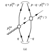
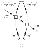
Figure 5: Feynman diagrams for the Green function of the $\eta^{\prime}$ propagation (a) after the first collision and (b) before the last collision. The solid, dashed, and wavy lines represent the nucleons, $\eta^{(\prime)}$ meson, and photon, respectively. The open circles and boxes are not included in the evaluation of the Green function. Three-momenta carried by the particles are shown (a) in the laboratory frame and (b) in the total center-of-mass frame.

Next, we fix the double scattering amplitude $\mathcal{T}_{p2}$. As in Fig. 4 ($p2$), we construct this with the deuteron wave functions at appropriate places, $\gamma p\to\eta^{\prime}p$ amplitude for the first collision, $pn\eta^{\prime}\to pn\eta^{\prime}$ amplitude, $\eta^{\prime}p\to\eta p$ amplitude, and two Green functions of the $\eta^{\prime}$ propagation: after the first collision and before the last collision.

Among them, the two Green functions can be evaluated by using the diagrams in Fig. 5. For the Green function after the first collision [Fig. 5(a)], the photon momentum should be shared by $\eta^{\prime}$ and two nucleons. Assigning the momenta $p_{\gamma}^{\rm lab}/3$ and $2p_{\gamma}^{\rm lab}/3$, where $p_{\gamma}^{\rm lab}=E_{\gamma}^{\rm lab}$, for the $\eta^{\prime}$ and deuteron in the multiple $\eta^{\prime}$ scattering in the laboratory frame, respectively, we can evaluate this Green function for the $\eta^{\prime}$ propagation as

$$G_{\eta^{\prime}}^{\rm first} =\int\frac{d^{3}q}{(2\pi)^{3}}\int\frac{d^{3}p}{(2\pi)^{3}}\frac{\tilde{\varphi}(q)\tilde{\varphi}(|\bm{q}-\bm{p}+2\bm{p}_{\gamma}^{\rm lab}/3|)}{p_{\eta^{\prime}}^{0}(W)^{2}-\bm{p}^{2}-m_{\eta^{\prime}}^{2}+i0}$$

$$=\int\frac{d^{3}p}{(2\pi)^{3}}\frac{F_{NN}(|\bm{p}-2\bm{p}_{\gamma}^{\rm lab}/3|)}{p_{\eta^{\prime}}^{0}(W)^{2}-\bm{p}^{2}-m_{\eta^{\prime}}^{2}+i0}.$$ (29)

The energy of the mediated meson $p_{\eta^{\prime}}^{0}(W)$ was defined in Eq. (9). For the Green function before the last collision [Fig. 5(b)], we need to bind two nucleons, one of which has a high momentum $\approx p_{\eta}^{\rm cm}$ coming from the mass difference between $\eta^{\prime}$ and $\eta$, to make the final-state deuteron. Therefore, the Green function before the last collision is

$$G_{\eta^{\prime}}^{\rm last}= \int\frac{d^{3}q^{\prime}}{(2\pi)^{3}}\int\frac{d^{3}p^{\prime}}{(2\pi)^{3}}\frac{\tilde{\varphi}(q^{\prime})\tilde{\varphi}(|\bm{q}^{\prime}+\bm{p}^{\prime}-\bm{p}_{\eta}^{\rm cm}/2|)}{p_{\eta^{\prime}}^{0}(W)^{2}-\bm{p}^{\prime\,2}-m_{\eta^{\prime}}^{2}+i0}$$

$$= \int\frac{d^{3}p^{\prime}}{(2\pi)^{3}}\frac{F(|\bm{p}^{\prime}-\bm{p}_{\eta}^{\rm cm}/2|)}{p_{\eta^{\prime}}^{0}(W)^{2}-\bm{p}^{\prime\,2}-m_{\eta^{\prime}}^{2}+i0}.$$ (30)

We note that, owing to the integrals, both the Green functions $G_{\eta^{\prime}}^{\rm first}$ and $G_{\eta^{\prime}}^{\rm last}$ do not depend on the directions of $\bm{p}_{\gamma}^{\rm lab}$ and $\bm{p}_{\eta}^{\rm cm}$, respectively, and they are functions only of the center-of-mass energy $W$.

Now we can formulate the scattering amplitude $\mathcal{T}_{p2}$ as

$$\mathcal{T}_{p2}= T_{\gamma p\to\eta^{\prime}p}(E_{\gamma}^{\rm lab})G_{\eta^{\prime}}^{\rm first}T_{22}^{\rm FCA}(W)G_{\eta^{\prime}}^{\rm last}T_{21}(w^{\rm FCA}(W)),$$ (31)

where $T_{21}$ is the $\eta^{\prime}N\to\eta N$ scattering amplitude in Sec. II.1 with its argument $w^{\rm FCA}$ in Eq. (7).

In a similar manner, we can evaluate the other amplitudes for the $\gamma d\to\eta d$ reaction:

$$\mathcal{T}_{p3}= T_{\gamma p\to\eta^{\prime}p}(E_{\gamma}^{\rm lab})G_{\eta^{\prime}}^{\rm first}T_{21}^{\rm FCA}(W)G_{\eta^{\prime}}^{\rm last}T_{21}(w^{\rm FCA}(W)),$$ (32)

$$\mathcal{T}_{n2}= T_{\gamma n\to\eta^{\prime}n}(E_{\gamma}^{\rm lab})G_{\eta^{\prime}}^{\rm first}T_{12}^{\rm FCA}(W)G_{\eta^{\prime}}^{\rm last}T_{21}(w^{\rm FCA}(W)),$$ (33)

and

$$\mathcal{T}_{n3}= T_{\gamma n\to\eta^{\prime}n}(E_{\gamma}^{\rm lab})G_{\eta^{\prime}}^{\rm first}T_{11}^{\rm FCA}(W)G_{\eta^{\prime}}^{\rm last}T_{21}(w^{\rm FCA}(W)).$$ (34)

Here we note that, because the scatterings of $p2$, $p3$, $n2$, and $n3$ take place in $s$ wave, the scattering amplitudes $\mathcal{T}_{p2,p3,n2,n3}$ do not depend on the scattering angle but only on $E_{\gamma}^{\rm lab}$. In the full amplitudes, the multiple scattering amplitude appears as the sum of the $\eta^{\prime}pn$ and $pn\eta^{\prime}$ contributions, i.e., $\mathcal{T}_{p2}+\mathcal{T}_{p3}\propto T_{21}^{\rm FCA}+T_{22}^{\rm FCA}$ and $\mathcal{T}_{n2}+\mathcal{T}_{n3}\propto T_{11}^{\rm FCA}+T_{12}^{\rm FCA}$.

III.2 Numerical Results

With the scattering amplitudes constructed in the previous subsection, we can calculate the cross section of the $\gamma d\to\eta d$ reaction. In the present study the spin components for the photon and baryons are irrelevant, so we can write the differential cross section omitting the average and summation of the polarizations as

$$\frac{d\sigma_{\gamma d\to\eta d}}{d\Omega}=\frac{m_{d}^{2}\,p_{\rm cm}^{\prime}}{16\pi^{2}p_{\rm cm}W^{2}}\left|\mathcal{T}_{\gamma d\to\eta d}\right|^{2},$$ (35)

where $p_{\rm cm}$ and $p_{\rm cm}^{\prime}=p_{\eta}^{\rm cm}$ denote the momenta of the photon and $\eta$ in the center-of-mass frame, respectively, and $m_{d}$ is the deuteron mass.

Figure 6: Differential cross section $d\sigma/d\Omega$ for the $\gamma d\to\eta d$ reaction with the photon energy $E_{\gamma}^{\rm lab}=669$–$688\text{ MeV}$ as a function of $\eta$ emission angle in the center-of-mass frame. The theoretical result is obtained at $E_{\gamma}^{\rm lab}=680\text{ MeV}$. The experimental data are taken from Ref. Weiss:2001yy (TAPS) and from Ref. HoffmannRothe:1997sv (PHOENICS).

Figure 7: Differential cross section $d\sigma_{\gamma d\to\eta d}/d\Omega$ for the $\gamma d\to\eta d$ reaction with scattering angles $\cos\theta_{\eta}^{\rm cm}=-1$, $-0.5$, $0$, $+0.5$, and $+1$. The solid lines denote the values for the full calculation, while the dotted and dashed lines are contributions from the impulse $\eta$ production and the multiple $\eta^{\prime}$ scattering, respectively.

Before showing the numerical results in the energy region of the $\eta^{\prime}d$ bound-state signal, we demonstrate that the coefficient for the coherent process $|A_{\rm IS}|/|A_{\rm IS}+A_{\rm IV}|=0.22$ [see Eq. (22)] can reproduce the $\gamma d\to\eta d$ cross section at slightly above the $\eta$ production threshold, e.g., $E_{\gamma}^{\rm lab}=680\text{ MeV}$. For this calculation, the $\gamma p\to\eta p$ amplitude is assumed to be constant independent of both the photon energy and scattering angle and is fitted to reproduce the cross section summarized by Bonn–Gatchina in the close-to-threshold region of $\eta$ production off the free proton, $E_{\gamma}^{\rm lab}\approx 708\text{ MeV}$. Other terms in the calculation of the $\gamma d\to\eta d$ amplitude are unchanged.

The numerical result is shown in Fig. 6 with the photon energy $E_{\gamma}^{\rm lab}=680\text{ MeV}$. As one can see from the comparison with the experimental data at $E_{\gamma}^{\rm lab}=669$–$688\text{ MeV}$, the cross section as well as the angular dependence is quantitatively reproduced. This means that the present formulation is appropriate with the coefficient $|A_{\rm IS}|/|A_{\rm IS}+A_{\rm IV}|=0.22$ and we do not need further normalization factors. In the following we use the same value even in the energy region of the $\eta^{\prime}d$ bound state.

Now we show the numerical results of the differential cross section for the $\gamma d\to\eta d$ reaction with the photon energies which may generate an $\eta^{\prime}d$ bound state in Fig. 7. The scattering angle is chosen to be $\cos\theta_{\eta}^{\rm cm}=-1$, $-0.5$, $0$, $+0.5$, and $+1$. We also plot contributions from the impulse $\eta$ production ($\mathcal{T}_{p1}+\mathcal{T}_{n1}$) and the multiple $\eta^{\prime}$ scattering ($\mathcal{T}_{p2}+\mathcal{T}_{p3}+\mathcal{T}_{n2}+\mathcal{T}_{n3}$).

Let us consider backward $\eta$ production with $\cos\theta_{\eta}^{\rm cm}=-1$. As one can see from the lowest panel of Fig. 7, the differential cross section is dominated by the multiple $\eta^{\prime}$ scattering contribution and the $\eta^{\prime}d$ bound-state signal is clear as a bump structure with its strength $\sim 0.2\text{ nb}/\text{sr}$. In backward $\eta$ production, single-step $\eta$ emission off a bound nucleon is highly suppressed because of a momentum mismatching between two nucleons in forming a deuteron. In this sense, backward $\eta$ production is of interest in searching for the signal of the $\eta^{\prime}d$ bound state. A similar tendency holds in the scattering angle $\cos\theta_{\eta}^{\rm cm}\leq 0$, where the cross section is dominated by the multiple $\eta^{\prime}$ scattering shown in dashed lines.

Next, as the $\eta$ is emitted at more forward angles, the single-step background contribution becomes much more significant. At $\cos\theta_{\eta}^{\rm cm}=+0.5$ the single-step contribution is comparable to the bound-state signal, and at $\cos\theta_{\eta}^{\rm cm}=1$ the single-step contribution is dominant. However, even at $\cos\theta_{\eta}^{\rm cm}=+0.5$ and $+1$, we can observe a bump structure coming from the $\eta^{\prime}d$ bound state. At $\cos\theta_{\eta}^{\rm cm}=+0.5$ the peak strength is approximately $0.5\text{ nb}/\text{sr}$, and at $\cos\theta_{\eta}^{\rm cm}=+1$ it is about $5\text{ nb}/\text{sr}$.

Here we should discuss two ambiguities in our amplitude. First, in the formulation of the $\gamma p\to\eta p$ and $\gamma n\to\eta n$ amplitudes, we suppressed the spin component as in Eq. (22). However, we used these amplitudes only to estimate the background contribution and to compare it with the signal strength of the $\eta^{\prime}d$ bound state. This background contribution was found to be negligible in backward $\eta$ production. Therefore, we will obtain the bound-state peak in backward $\eta$ production even if we take into account the spin component rigorously.

Second, as mentioned below Eq. (22), we fixed the $\gamma p\to\eta p$ amplitude as real quantities and did not introduce any explicit relative phase between the single-step amplitude and multiple $\eta^{\prime}$ amplitude. An important point is that the relative phase affects the structure for the bound state in forward $\eta$ production. The bump structure at $\cos\theta_{\eta}^{\rm cm}=+0.5$ and $+1$ in Fig. 7 is determined by the constructive interference between the bound-state formation and the single-step background contribution. Such a pattern of the interference may change owing to the phases of the underlying reactions. For instance, if we introduce a relative phase $e^{i\pi}=-1$, a bump in forward $\eta$ production seen in Fig. 7 would become a dip structure due to the destructive interference. Besides, the bound-state signal in backward $\eta$ production will be almost independent of the relative phase between the single-step amplitude and multiple $\eta^{\prime}$ one, because the multiple $\eta^{\prime}$ scattering dominates the cross section and the interference is negligible. In this sense, we may experimentally discuss the relative phase as well as the strength of the bound-state signal by investigating the angular dependence of the cross section.

Figure 8: Differential cross section $d\sigma/d\Omega$ for the $\gamma d\to\eta d$ reaction with several values of the parameter $g$ in the $\eta^{\prime}N\to\eta^{\prime}N$ interaction (1). The scattering angle is fixed as $\cos\theta_{\eta}^{\rm cm}=-1$.

Before closing this section, we briefly discuss how the signal of the $\eta^{\prime}d$ bound state in the $\gamma d\to\eta d$ reaction changes in case of slightly smaller or larger binding energies of the $\eta^{\prime}d$ system. For this purpose, we vary the strength of the $\eta^{\prime}N$ interaction via the parameter $g$ in Eq (1), which is the coupling constant for the $\sigma NN$ vertex. We plot in Fig. 8 the differential cross section at the scattering angle $\cos\theta_{\eta}^{\rm cm}=-1$ with parameters $g=6.0$, $7.0$, $8.0$, and $9.0$, which generate the $\eta^{\prime}d$ bound state with its poles at $2832-2i$, $2821-6i$, $2801-11i$, and $2775-17i\text{ MeV}$, respectively. As one can see, when the coupling constant $g$ is smaller, i.e., the $\eta^{\prime}N$ interaction is weaker, the strength of the $\eta^{\prime}d$ bound-state signal decreases as well. On the other hand, a larger coupling constant $g$ brings a similar strength of the bound-state signal $\sim 0.2\text{ nb}/\text{sr}$ compared to that in the case of the original parameter.

IV Summary

We theoretically investigated a possibility of binding an $\eta^{\prime}d$ system by an attractive strong interaction between $\eta^{\prime}$ and nucleons. Thanks to the attractive nature of the $\eta^{\prime}N$ interaction from the linear $\sigma$ model, which is an effective model respecting chiral symmetry of QCD, the $\eta^{\prime}d$ system can be bound in this model. With the fixed center approximation to the Faddeev equation, its binding energy measured from the $\eta^{\prime}d$ threshold and decay width are $25\text{ MeV}$ and $19\text{ MeV}$, respectively.

We then proposed the $s$-channel formation of the $\eta^{\prime}d$ bound state in the $\gamma d\to\eta d$ reaction at the center-of-mass energy $\approx 2.8\text{ GeV}$, corresponding to the photon energy $E_{\gamma}^{\rm lab}\approx 1.2\text{ GeV}$. A clear peak structure with the strength of $\sim 0.2\text{ nb}/\text{sr}$ for the signal of the $\eta^{\prime}d$ bound state was observed in backward $\eta$ emission, thanks to large suppression of a background coming from single-step $\eta$ emission off a bound nucleon. In addition, the bound-state signal may manifest itself even in forward $\eta$ emission as a bump or a dip, which depends on the interference between the bound-state formation and the single-step background.

This result motivates a new experimental program Fujioka:2017LOI using the tagged photon beam Ishikawa:2010zza and the FOREST detector Ishikawa:2016kin at the Research Center for Electron Photon Science (ELPH), Tohoku University, Japan.