Combination of analysis techniques for efficient track reconstruction in high multiplicity events

Abstract

A novel combination of established data analysis techniques for reconstructing all charged-particle tracks in high energy collisions is proposed. It uses all information available in a collision event while keeping competing choices open as long as possible. Suitable track candidates are selected by transforming measured hits to a binned, three- or four-dimensional, track parameter space. It is accomplished by the use of templates taking advantage of the translational and rotational symmetries of the detectors. Track candidates and their corresponding hits, the nodes, form a usually highly connected network, a bipartite graph, where we allow for multiple hit to track assignments, edges. The graph is cut into very many minigraphs by removing a few of its vulnerable components, edged and nodes. Finally the hits are distributed among the track candidates by exploring a deterministic decision tree. A depth-limited search is performed maximising the number of hits on tracks, and minimising the sum of track-fit $\chi^{2}$. Simplified models of LHC silicon trackers, as well as the relevant physics processes, are employed to study the performance (efficiency, purity, timing) of the proposed method in the case of single or many simultaneous proton-proton collisions (high pileup), and for single heavy-ion collisions at the highest available energies.

1 Introduction

Traditional methods of track reconstruction can be scaled to work in high multiplicity events, namely in many simultaneous collisions (pileup) of elementary particles Aad:2015ina ; Rovere:2015rep and in high multiplicity single heavy-ion collisions. Nevertheless the performances are not optimal, efficiency and purity are reduced, especially at low momentum. That is why present data taking conditions and further luminosity and energy upgrades of high energy particle colliders, as well as those of detector systems, call for new ideas.

Image transformation methods and neural networks Fruhwirth:1993wv are often used in gaseous detectors (time projection chambers Aamodt:2008zz ; Cheshkov:2006ym and transition radiation trackers Aad:2008zzm ; Mindur:2017nqn ). In the case of silicon trackers the combinatorial track finding methods employed for trajectory building mostly use local information Strandlie:2004ig ; Chatrchyan:2008aa . They start with a trajectory seed and build the trajectory by extending the seed through the detector layers, picking up compatible hits. In the case of very many compatible hits the number of concurrently built trajectory candidates must be limited. Only some of the best candidates are kept which biases the final result. In this sense, decisions are made too early. Moreover, trajectories are mostly treated separately, there is no interaction between their assigned hits.

In this study a combination of established data analysis techniques for the offline reconstruction of all charged-particle trajectories is proposed. It uses all information available in an event while keeping competing choices open as long as possible. Details of silicon detectors, relevant physical effects and tracking with Kalman filter are introduced in Sec. 2. Pattern recognition along with the preparation of templates, image transformation, and trajectory building are discussed in Sec. 3. The optimal distribution of hits among tracks with help of graph-theoretic methods are shown in Sec. 4. Results of simulations based on simplified but realistic models of silicon trackers at particle colliders are detailed in Sec. 5, where the performance (efficiency, purity, timing, parallelisation) of the proposed methods are displayed.

Table 1: The main characteristics of the inner barrel silicon detectors of the studied experimental setups. The value of the longitudinal magnetic field $B_{z}$ is shown along with layer type, radii of barrel cylinders, tilt angle (in case of double-sided strips), spatial resolution of hits in $r\phi$ and $z$ directions, and material thickness $x/X_{0}$ in radiation length units. In the case of strips the strip length $l_{z}$ is given instead, in parentheses.

	$B_{z}$ [T]	Layer type	Radii [cm]	Tilt [mrad]	$\sigma_{r\phi}$	$\sigma_{z}$ ($l_{z}$)	$x/X_{0}$ [$\%$]
Exp A	2.0	pixels	5.0, 8.8, 12.2	–	10 $\mathrm{\mu}m$	115 $\mathrm{\mu}m$	4
		strips	29.88, 29,92	$\pm 20$	17 $\mathrm{\mu}m$	(6.4 cm)	2
		strips	37.08, 37,12	$\pm 20$	17 $\mathrm{\mu}m$	(6.4 cm)	2
		strips	44.28, 44,32	$\pm 20$	17 $\mathrm{\mu}m$	(6.4 cm)	2
Exp B	0.4	pixels	3.9, 7.6	–	12 $\mathrm{\mu}m$	100 $\mathrm{\mu}m$	1
		drifts	14.9, 23.8	–	35 $\mathrm{\mu}m$	25 $\mathrm{\mu}m$	1
		strips	38.48, 38.52	$+7.5,-27.5$	20 $\mathrm{\mu}m$	(4 cm)	0.5
		strips	43.58, 43.62	$+7.5,-27.5$	20 $\mathrm{\mu}m$	(4 cm)	0.5
Exp C	3.8	pixels	4.4, 7.3, 10.2	–	15 $\mathrm{\mu}m$	15 $\mathrm{\mu}m$	3
		strips	25.48, 25,52	$\pm 50$	23 $\mathrm{\mu}m$	(10 cm)	2
		strips	33.88, 33.92	$\pm 50$	23 $\mathrm{\mu}m$	(10 cm)	2
		strips	41.8	0	35 $\mathrm{\mu}m$	(10 cm)	2
		strips	49.8	0	35 $\mathrm{\mu}m$	(10 cm)	2

2 Silicon detectors at particle colliders

At currently operating particle colliders the interaction region is very narrow (of the order of $50\,\mathrm{\mu}m$) in transverse direction, while in $z$ (longitudinal or beam) direction it is long, with a characteristic size of about 10 cm MLamont . For single heavy-ion collisions the $z_{0}$ position of the primary interaction (vertex) is estimated with good precision using the copiously produced high transverse-momentum particles, thanks to the small pointing uncertainty of their tracks, reconstructed with traditional methods. In the case of single or multiple pp collisions no such information on the locations of the interaction vertices exists.

The trajectory of a primary particle is primarily determined by its initial position $(0,0,z_{0})$ and parameters $(q,\eta,p_{\text{T}},\phi_{0})$ of its initial momentum at creation. Here $q$ is the charge, $\eta=-\ln\tan(\theta_{0}/2)$ is the pseudorapidity, $p_{\text{T}}$ is the transverse momentum, $\phi_{0}$ and $\theta_{0}$ are the azimuthal and polar angles of the initial momentum vector in spherical coordinates. In a large volume solenoid the magnetic field near the center of the detector is rather homogeneous and points in the $z$ direction. Hence in small volumes the trajectories of charged particles can be approximated by piecewise helices. For practical purposes a primary particle is parametrised by $(k_{\text{T}},\sinh\eta,\phi_{0},z_{0})$ in the following, where $k_{\text{T}}=q/R$ is the signed curvature of the projection of its trajectory on the transverse (bending) plane, $R$ is its radius. If the particle is singly charged the curvature is connected to $p_{\text{T}}$ as $p_{\text{T}}=eB_{z}R$, where $e$ is the electric charge of a proton, $B_{z}$ is the value of the longitudinal magnetic field.

The central parts of silicon trackers generally consist of several concentric cylindrical layers. Those close to the nominal interaction point are equipped with tiny pixel sensors, while others contain long strip sensors parallel with the beam direction. Some strip layers are double-sided, they are located very close to each other two by two, and have a small relative tilt angle. The main characteristics of the inner barrel silicon detectors of the studied experimental setups are given in Table 1.

The trajectory of the primary particle intersects the concentric cylindrical layers and leaves hits behind in the silicon (Fig. 1). In the simplified case, when the magnetic field is homogeneous and if the detector material and its physical effects are neglected, the position of those hits could be precisely determined by simple equations. The physical effects of detector material changes this overly simple picture.

Figure 1: Left: pixel hits (red open squares) and strip hits (red solid line sections) of a single inelastic pp collision from the simulation of Exp B. The location of the primary interaction is plotted with a green circle, the beamline is indicated by a gray straight line. Charged particle trajectories (blue dashed curves) are also plotted. Right: event with 40 simultaneous inelastic pp collisions from the simulation of Exp C.

2.1 Physical effects

When a long lived charged particle propagates through material the most important effects which alter its momentum vector are multiple scattering and energy loss. The distribution of multiple Coulomb scattering is roughly Gaussian Olive:2016xmw , the standard deviation of the planar scattering angle is

$$\theta_{0}=\frac{13.6~{}\text{MeV}}{\beta cp}z\sqrt{x/X_{0}}\bigl{[}1+0.038\ln(x/X_{0})\bigr{]},$$ (1)

where $p$, $\beta c$, and $z$ are the momentum, velocity, and charge of the particle in electron charge units, and $x/X_{0}$ is the thickness of the scattering material in radiation lengths.

Momentum and energy is lost during traversal of sensitive detector layers and support structures. To a good approximation the most probable energy loss $\Delta_{p}$, and the full width of the energy loss distribution at half maximum $\Gamma_{\Delta}$ Bichsel:1988if are

$$\Delta_{p} =\xi\left[\ln\frac{2mc^{2}\beta^{2}\gamma^{2}\xi}{I^{2}}+0.2000-\beta^{2}-\delta\right],$$ (2)

$$\Gamma_{\Delta} =4.018\xi,$$ (3)

where $\xi=\frac{K}{2}z^{2}\frac{Z}{A}\rho\frac{x}{\beta^{2}}$ is the Landau parameter; $K=4\pi N_{A}r_{e}^{2}m_{e}c^{2}$; $m$ is the mass of the particle; $Z$, $A$, $I$, and $\rho$ are the mass number, atomic number, excitation energy, and the density of the material, respectively Olive:2016xmw . The density correction $\delta$ is neglected.

2.2 Hit clusters

An incoming charged particle loses energy in the sensitive detector elements by producing electron-hole pairs. The neighboring channels collecting a charge above a given threshold are grouped to form a cluster, a reconstructed hit. The size (dimensions) of the cluster depends on the angle of incidence of the particle: bigger angles result in larger clusters. The expected cluster dimensions in $r\phi$ and $z$ directions in pitch units are

$$m_{r\phi} =\frac{t_{r}|\tan\psi|}{t_{r\phi}}, m_{z} =\frac{t_{r}|\tan\theta|}{t_{z}},$$

where $\theta$ and $\psi$ are local angles (Sec. 2.3), $t_{r}$ is the thickness of the layer in radial direction, while $t_{r\phi}$ and $t_{z}$ are the dimensions of sensitive elements, pitches, in azimuthal ($r\phi$) and longitudinal ($z$) directions, respectively. For simplicity, the values $t_{r}=300\,\mathrm{\mu}m$, $t_{r\phi}=100\,\mathrm{\mu}m$, and $t_{z}=200\,\mathrm{\mu}m$ are chosen in the simulation (Sec. 5) for each experimental setup. Due to the large fluctuations in energy loss, the measured $w_{r\phi}$ and $w_{z}$ dimensions of the clusters differ from the expected ones. In order to model these effects in the simulation, the cluster dimensions are varied by one unit in both directions for pixels, and up and down by two units in $r\phi$ direction for strips.

If the size of a pixel cluster is at least two units in both directions, the layout of its pixels with charge deposit and its location relative to the nominal interaction point usually indicate the sign of the electric charge of the particle (Fig. 2). This way a pixel cluster is characterised by the measured widths $w_{r\phi}$ and $w_{z}$ (dimensions of its rectangular envelope), and the charge $q$, which can be $1$ or $-1$, or left unknown. A strip cluster has only one such quantity, its $w_{r\phi}$ width.

2.3 Particle tracking

The Kalman filter is widely used in particle physics experiments for charged track and vertex finding and fitting, and provides a coherent framework for handling known physical effects and measurement uncertainties Fruhwirth:1987fm . It is equivalent to a global linear least-squares fit which takes into account all correlations coming from process noise. It is the optimum solution since it minimises the mean square estimation error.

Figure 2: Illustration of the connection between the hit cluster shape and the local momentum vector, as well as the electric charge of the particle. The low-momentum positively charged particle (red) leaves a cluster with dimensions $(3,3)$, in pitch units, in the pixel detector. The fast charged particle (blue) induces a smaller $(2,1)$ cluster; in this case the electric charge cannot be unambiguously determined.

The state vector $\vec{x}=(\kappa,\theta,\psi,r\phi,z)$ is five dimensional:

$$\kappa =q/p \text{(signed inverse momentum)},$$

$$\theta =\theta(\vec{p}) \text{(local polar angle)},$$

$$\psi =\phi({\vec{p}}) \text{(local azimuthal angle)},$$

$$r\phi =r\phi({\vec{r}}) \text{(global azimuthal position)},$$

$$z =r_{L} \text{(global longitudinal position)}.$$

The propagation function $\vec{f}(\vec{x})$ from layer to layer is calculated analytically using a helix model. Multiple scattering and energy loss in tracker layers is implemented with their Gaussian approximations shown in Eqs. (1)–(3). The propagation matrix $F=\partial\vec{f}/\partial\vec{x}$ is obtained by numerical derivation. The measurement vector for pixel hits $\vec{m}=(r\phi,z)$ is two dimensional, for strip hits $\vec{m}=(r\phi)$ it is one dimensional. The measurement operator for pixels is

$$H=\begin{pmatrix}0&0&0&1&0\\ 0&0&0&0&1\end{pmatrix}.$$

while for strips it is

$$H=\begin{pmatrix}0&0&0&1&-\tan\alpha\end{pmatrix}.$$

The covariance of the process noise $Q$ is

$$Q=(F_{\kappa}\otimes F_{\kappa}^{T})\sigma_{\kappa}^{2}+(F_{\theta}\otimes F_{\theta}^{T})\sigma_{\theta}^{2}+(F_{\psi}\otimes F_{\psi}^{T})\sigma_{\psi}^{2}$$

where $\sigma_{\kappa}=\kappa\sigma_{\Delta}/\beta$, $\sigma_{\theta}=\sigma_{\psi}=\theta_{0}$ and $F_{a}=\partial\vec{f}/\partial x_{a}$ is a vector. Multiple scattering contributes both to the variation of $\theta$ and $\psi$, while energy loss affects only $\kappa$.

The covariance of measurement noise $V$ for pixels is

$$V=\begin{pmatrix}\sigma_{r\phi}^{2}&0\\ 0&\sigma_{z}^{2}\end{pmatrix}.$$

Figure 3: Left: distributions of $\phi-\phi_{0}$ differences of the hit and track azimuth angles as a function of $k_{\text{T}}$ for some selected detector layers. Right: distributions of $z-z_{0}$ differences of the hit and track longitudinal coordinates as a function of $\sinh\eta$ for some selected detector layers. Values from simulation of Exp C are plotted with various symbols, while the oversimplified expectations $\phi-\phi_{0}\approx-\arcsin(r/2\cdot k_{\text{T}})$ and $z-z_{0}\approx 2\sinh\eta\cdot\arcsin(r/2\cdot k_{\text{T}})/k_{\text{T}}$ at $k_{\text{T}}=0.01~{}\mathrm{cm^{-1}}$ are shown with the curves.

In the case of strips with $\alpha$ tilt angle, the inverse of the covariance matrix is

$$V^{-1}=R(\alpha)\begin{pmatrix}1/\sigma_{r\phi}^{2}&0\\ 0&0\end{pmatrix}R^{T}(\alpha)\approx\frac{1}{\sigma_{r\phi}^{2}}\begin{pmatrix}1-\alpha^{2}&-\alpha\\ -\alpha&\alpha^{2}\end{pmatrix}$$

where $R(\alpha)$ is a rotation matrix.

Table 2: Ranges and the optimised number of bins (working point) corresponding to track parameters. The value of $p_{\text{T,min}}$ is 0.1 GeV/$c$.

Variable	Range	Bins
$k_{\text{T}}$	$[-eB_{z}/p_{\text{T,min}},eB_{z}/p_{\text{T,min}}]$	50
$\sinh\eta$	$[-\sinh 1.5,\sinh 1.5]$	100
$\phi_{0}$	$[-\pi,\pi]$	200
$z_{0}$	$[-3\sigma_{z},3\sigma_{z}]$	50

Simulated particles are tracked while they are in the volume of the tracker detector, that is, trajectories looping in the magnetic field are properly followed. In the case of pattern recognition and track reconstruction only inside-out propagation is considered.

3 Pattern recognition

Our goal is to collect as much information as possible about potential track candidates, based on the location and shape of the measured hits in an event. To accomplish this, the position of each hit is transformed to a four-dimensional $(k_{\text{T}},\sinh\eta,\phi_{0},z_{0})$ accumulator space of track parameters. The accumulator space is not continuous but binned. (Bins are consecutive, adjacent, non-overlapping equal size intervals of a variable.) Ranges and the optimised number of bins corresponding to track parameters are shown in Table 2. The transformation is a variant of the well-known Hough transform hough1962method . In the absence of physical effects (Sec. 2.1) the image of a point-like $(r\phi,z)$ hit would be a well-defined two-dimensional manifold in that space, while the image of a section-shaped strip hit would be a three-dimensional manifold.

3.1 Preparation of templates

The detector models studied here have translational symmetry in longitudinal ($z$) and rotational symmetry in azimuthal ($r\phi$) direction. The $\phi-\phi_{0}$ angular difference primarily depends on $k_{\text{T}}$, while the $z-z_{0}$ longitudinal difference is mostly a function of $\sinh\eta$ (Fig. 3). These difference distributions further depend on the shape of the hit cluster (Sec. 2.2). For particles with a given $(k_{\text{T}},\sinh\eta)$ and mass, the $(\phi-\phi_{0},z-z_{0})$ values on a given detector layer populate a small rectangular area. The dimensions of that area result from the binning of the track parameters.

With help of numerous simulated particles we determine the populated area with help of local linear approximations

$$\begin{pmatrix}\phi-\phi_{0}\\ z-z_{0}\end{pmatrix}=\begin{pmatrix}\phi-\phi_{0}\\ z-z_{0}\end{pmatrix}_{c}+\frac{\partial(\phi-\phi_{0},z-z_{0})}{\partial(k_{\text{T}},\sinh\eta)}\begin{pmatrix}\Delta k_{\text{T}}\\ \Delta\sinh\eta\end{pmatrix}$$

around the center of each $(k_{\text{T}},\sinh\eta)$ bin. In practice the $(\cdot)_{c}$ central values and the $\partial(\cdot)/\partial(\cdot)$ Jacobian is deduced for each bin. The set of these values will be referred to as templates in the following.

In order to have uniform coverage in all bins, the distribution of simulated particles is chosen to be constant in $k_{\text{T}}$, $\sinh\eta$, and $\phi_{0}$. To limit fluctuations, normally distributed random variables, used in the simulation of physics processes (Sec. 2.1), are limited to values within 3.5 standard deviations (only about 0.05% lies outside this range). Altogether $2\times 10^{6}$ pions are generated.

The role and use of cluster shape information is shown through the distribution of template values (their width in $\phi$ direction) as a function of $(k_{\text{T}},\sinh\eta)$ in Fig. 4.

The prepared templates are used in two ways. During the early stage of image transformation they provide a $(\phi_{0},z_{0})$ accumulator area to increment for each (pixel) hit, in the case of a given $(k_{\text{T}},\sinh\eta)$ bin. Later they are used to specify a search rectangle on the $(r\phi,z)$ plane of a (strip) layer for a given $(k_{\text{T}},\sinh\eta,\phi_{0},z_{0})$ bin.

Although detector models with only barrel silicon detectors are studied here, the above considerations can be adopted to other geometries, such as disks perpendicular to the beam axis. In that case, the translational symmetry would be lost and the templates would become more complex by introducing another dimension, namely the relative $z$ position of the primary interaction with respect to the longitudinal coordinate of the disk.

3.2 Image transformation

The transformation of spatial information to track space proceeds as described in the following. First hits on the three innermost layers are dealt with, containing exclusively pixel hits. For each hit all potential $(k_{\text{T}},\sinh\eta)$ accumulator bins are examined and the corresponding possible $(\phi_{0},z_{0})$ values, enveloped by rectangles, are determined. Bins within such $(k_{\text{T}},\sinh\eta,\phi_{0},z_{0})$ area are incremented. Since we look for tracks with hits on all three innermost layers, only those accumulator bins are kept which gathered votes from all three layers.

Figure 4: The role and use of cluster shape information is shown through the distribution of template values (their width in $\phi$ direction) as a function of $(k_{\text{T}},\sinh\eta)$. The clusters with given $(w_{r\phi},w_{z})^{q}$ shape values are taken from a given pixel layer. For better discrimination between the three cluster shapes, the projections of their set of points are also shown on the base with light colour.

The subsequent layers usually contain strip hits. The method used for the innermost layers would not be efficient here because there are far too many accumulator bins to handle. To this end, the kept accumulator bins are examined, corresponding to proto-tracks with three counts, obtained in the previous step. Using the bin coordinates $(k_{\text{T}},\sinh\eta,\phi_{0},z_{0})$ we look for compatible hits by determining a search rectangle on the $(r\phi,z)$ plane for each layer. For quick access, and in order to facilitate hit selection, strip hits are in advance partitioned on an equidistant grid using their $(r\phi,z)$ coordinates.

Figure 5: Distribution of hit images (red dots) in $(k_{\text{T}},\sinh\eta,\phi_{0})$ accumulator space in the case of a single pp collision for a given $z_{0}$ value. The found track candidates are marked with blue boxes.

The search for compatible hits proceeds outwards. It is advantageous since the process can be abandoned if some layers provided no compatible hits while they are still reachable according to the curvature range of the examined bin. In other words, the number of layers with compatible hits should not be very different from the number of reachable layers. (We can allow for a few layers without hits.)

3.3 Trajectory building

Track candidates are built using hit images collected in given accumulator bins (Fig. 5). Trajectory propagation and track fitting is performed by the extended classical Kalman filter Fruhwirth:1987fm including prediction, filtering, and smoothing, with pion mass assumption. The initial state vector is estimated by placing a helix to the innermost two hits and using the beamline as a constraint by adding a zeroth point with value $r\phi=0$, and with an uncertainty of $\sigma_{r\phi}\approx 50\,\mathrm{\mu}m$. In the case of an off-centered beam, $\sigma_{r\phi}$ can be increased to properly contain the interaction region in the transverse plane.

Trajectory building normally proceeds from inside out and considers all hit combinations recursively by forming branches. At each layer there are usually multiple hits to add to the existing trajectory. The number of hits to be considered is especially large for the inner strip layers that would exponentially increase the number of trajectory branches.

A powerful solution for this problem is the effective detection of unsuitable (outlier) hits in the busy detector layers. For this purpose, trajectory building starts with the estimate of the initial state vector at the zeroth point, which is then propagated through the first three layers. At that point we already have a good knowledge about the parameters of the track that is being reconstructed. Instead of going to the next (strip) layer, the trajectory is at once propagated to one of the potential hits in the outermost detector layer (Fig. 6). During propagation the physical effects of the crossed layers are duly taken into account but information about their hits is not used. Next, the outliers in the intermittent omitted layers are detected in the smoothing step of the deficient trajectories using the smoothed residual Fruhwirth:1987fm . Hits in the upper 0.5% tail of the corresponding $\chi^{2}$ distribution are discarded.

Figure 6: Hits (red boxes and line sections) belonging to a given bin in the accumulator space and trajectories propagated to the outermost detector layer (blue dashed curves). The beamline is indicated with the gray straight line.

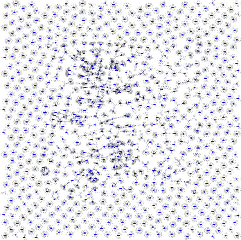
Figure 7: The bipartite graph $G$ of hits (black ellipses) and track candidates (blue diamonds) for an event with multiple (40) pp collisions. Directed arrows, graph edges, show potential hit-to-track candidate assignments. Filled diamonds indicate true tracks, while open ones show candidates where one or more hits are not in place.

Once the list of compatible strip hits is narrowed down, full trajectory building with the selected hits is performed again. During trajectory building we can allow for a few (one or two) missing hits. It may mean no hit at all or too large $\chi^{2}$ for a given number of degrees of freedom (ndf). If there are too many missing hits, the process is abandoned. In order not to lose a noticeable amount of track candidates, but also to have a good selection power, trajectories in the upper 0.5% tail of the corresponding $\chi^{2}$ distribution are discarded and not developed further (roughly those with $\chi^{2}\lesssim 1.7~{}\mathrm{ndf}+8.0$ are kept).

4 Optimal distribution of hits among tracks

In the end we have a set of track candidates with the somewhat unusual property that temporarily several track candidates may share some hits. Our goal is to resolve these ambiguities, hit confusion, by optimally allocating the hits among tracks, since all hits must be assigned to not more than one track. (The tasks is called optimal packing in mathematics.) The hits and track candidates, and their relations, are best represented by a bipartite graph $G$. The nodes of $G$ are from two disjoint sets: hits and track candidates, such that each edge connects a hit to a track candidate (Figs. 7 and 8). Our goal is to assign all hits to at most one track, while keeping an eye on the total goodness-of-fit of all tracks ($\sum\chi^{2}$) in the event.

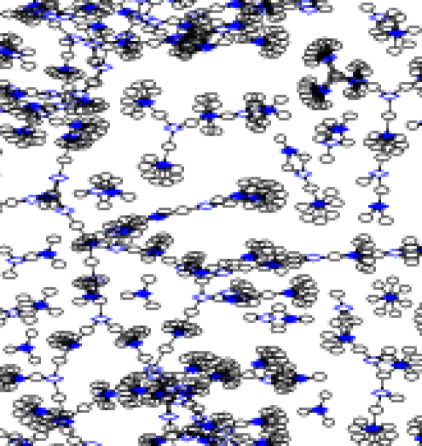
Figure 8: A small fraction of the bipartite graph $G$ of hits (black ellipses) and track candidates (blue diamonds) for an event with multiple (40) pp collisions. Directed arrows, graph edges, show potential hit-to-track candidate assignments. Filled diamonds indicate true tracks, while open ones show candidates where one or more hits are not in place.

First those track candidates are privileged which are very likely real. To this end, we extract a subgraph by selecting track candidates which have at least three hits not requested by other candidates, that is, at least three leaf hit nodes. (A leaf hit node is connected to exactly one track candidate node.) This subgraph is disconnected (Sec. 4.1), the arising minigraphs are solved (Sec. 4.2) individually. Selected tracks and stored, edges and nodes of the subgraph are removed from $G$. Next we extract the subgraph containing track candidates with the highest maximum number of possible hits (usually $n=9$), and their corresponding hits. Thanks to the high number of hits required, these track candidates are likely real. Selected tracks are again stored, nodes and edges removed from $G$ as above. Then the process is restarted with the subgraph of track candidates with $n-1$ hits, iterating down to the subgraph of track candidates with three hits.

4.1 Disconnecting a subgraph

The graphs encountered are usually highly connected. If we would try to allocate the hits to tracks one by one, the number of trials needed would explode exponentially with increasing number of nodes. In order to reduce the complexity of the problem, the graphs should be partitioned into several small pieces. This can be accomplished by finding some vulnerable components in the graph whose removal disconnects the graph. Such weak elements are special edges (bridges) and special nodes (articulation points) whose deletion increases the number of connected components of the graph. Of course this way some tracks would lose a hit, but that is only a small price to pay.

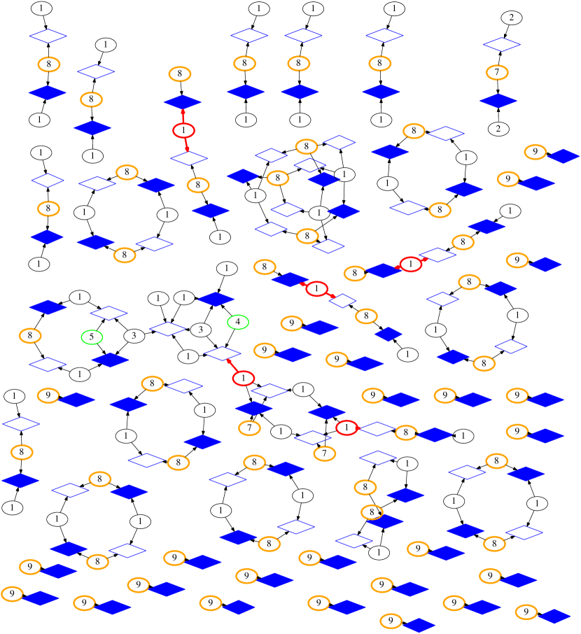
Figure 9: Example minigraphs obtained after the removing most of bridges and articulation points from the bipartite graph $G$ of hits and track candidates, in the case of an event with multiple (40) pp collisions. The thickness and colour of contracted hits (ellipses) refer the number of hits with identical role they represent (orange – 6 or more, green – 4 or 5, black – 3 or less), that number is printed within the corresponding ellipses. Filled diamonds indicate true tracks, while open ones show candidates where one or more hits are not in place. The remaining bridges and articulation points are drawn with thick red arrows and ellipses, respectively.

Bridges and articulation points can be found in linear time with help of graph traversal techniques. The depth-first search is an algorithm for traversing and searching a graph. One starts at some arbitrary node as the root and explores as far as possible along each branch before backtracking. The nodes of bridges and the articulation points are found by requiring that their children nodes do not have a backedge.

In a “disconnecting” step the found bridges and articulation points are removed. During the process new vulnerable elements may come to light, hence the disconnecting steps are repeated until no new such elements are found. As a next step, the resulted graph is further partitioned into disjoint graphs. This task is best accomplished by the flood fill method embedded into the above detailed traversal technique. The output of the disconnecting step is a large set of disjoint minigraphs.

In high-pileup pp events there are usually several thousand track candidates. Their corresponding bipartite graph $G$ and its subgraphs contain several hundred bridges and up to 50 articulation points. Once the subgraphs are disconnected, we get couple of thousand minigraphs.

4.2 Solving a minigraph

A minigraph usually has several hits with identical role: they are connected to the same set of track candidates. (Their number is between 2 and 7 hits for the detector models studied here.) In the interest of reducing complexity, hits with identical role are treated jointly, the set of such hits gets “contracted”.

The number of remaining nodes is usually small (Fig. 9), the contracted hits can be distributed among tracks by building and solving a decision tree. The process is similar to exploring decision trees of deterministic strategy board games, such as chess and go, including their horizon problem (limited search depth). What is different here is that our process is a single-player one. The optimal hit-to-track assignments are chosen in the following way, recursively:

Figure 10: Comparisons of track-fit $\chi^{2}$ distributions of track candidates (top) and of final tracks (bottom) for events with multiple pp collisions. Distributions from data (histograms) and compared to theoretical expectations (curves) for tracks with given number of degrees of freedom (ndf).

1. First the most important, highest ranked available (contracted) hit is located. Rank is calculated as the product of the number of similar hits (the number of hits the contracted hit represents) and the number of edges the hit node has (the number of associated track candidates). Such a definition gives preference to contracted hits which represent many particle hits and have a central role in the graph.

2. The highest ranked hit can be attached to several track candidates, and these choices are evaluated sequentially and recursively as branches of a decision tree. After a hit-track assignment is chosen, the track and its hits are selected, and their nodes and all corresponding edges are removed from the minigraph.

3. Track candidate nodes and corresponding edges with too few remaining hits (less than three) and those with too many missing hits are also removed.

4. As long as there are nodes left in the minigraph we go back to step 1, otherwise the actual path of the decision tree is evaluated based primarily on the amount of hits on selected tracks. If there are two decision trees with the same amount of hits, the one with lower $\sum\chi^{2}$ of the selected tracks is chosen.

In order to save time during solving the decision tree, the selected tracks candidates are not re-fitted but only the adjusted $\chi^{2}$ values of their remaining hits, calculated based on a Kalman-fit using all the initial hits, are summed and the corresponding ndf values are recalculated.

In the end the decision path with the best score is taken, the selected tracks and their hits are stored.

5 Results

In the computer simulation the interaction region is centered at $(x,y,z)=(0,0,0)$. In $z$ (beam) direction it is described by a Gaussian distribution with a standard deviation of $\sigma_{z}=$ 5 cm. The silicon tracker covers the pseudorapidity range of $|\eta|<1.5$.

Inelastic pp collisions at $\sqrt{s}=$ 14 TeV are obtained from the Pythia8 Sjostrand:2007gs Monte Carlo event generator (version 219). It is known to well reproduce the measured momentum spectrum of charged particles in pp collisions at $\sqrt{s}=$ 13 TeV Khachatryan:2015jna ; Adam:2015pza ; Aad:2016mok with an average pseudorapidity density of $dN/d\eta\approx 5.5$ near $\eta\approx 0$, as well as the composition of the most abundant charged particles (pions, kaons, protons). Semi-central PbPb collisions at $\sqrt{s_{\text{NN}}}=$ 5.5 TeV with $dN/d\eta\approx 1000$ are obtained from the Hydjet Lokhtin:2005px Monte Carlo event generator (version 1.9). It was tuned to match the measured momentum spectrum of charged particles in the highest energy heavy ion collisions, as seen for $\sqrt{s_{\text{NN}}}=$ 5.02 TeV energy central PbPb collisions Adam:2015ptt .

Physical effects (multiple scattering and energy loss) are simulated according to the simple models detailed in Sec. 2.1 using the description of detector materials shown in Table 1.

Figure 11: Performance of the proposed algorithm as a function of transverse momentum ($p_{\text{T}})$ of the charged particles. Efficiency (left) and fake track rate (right) are plotted for Exp A (top), Exp B (middle), and Exp C (bottom). The values are separately given for single pp (green triangles), multiple (40) pp (red circles), and semi-central PbPb (blue boxes) collisions. The horizontal scale is linear in the region 0–1 GeV/$c$, while it is logarithmic for 1–10 GeV/$c$. In the case of Exp C, values for single pp events from Sirunyan:2017zmn are shown for comparison with light green bands.

Comparisons of track-fit $\chi^{2}$ distributions of initial track candidates and of final tracks for events with multiple pp collisions are shown in Fig. 10. Distributions from data and compared to theoretical expectations for tracks with given number of degrees of freedom. While track candidates have distorted $\chi^{2}$ distributions, those of final tracks are much closer to the expected curves.

The proposed algorithm was coded in C++ and run on a 3.1 GHz quad-core computer. The average CPU time needed was on average 13 sec for events with 40 simultaneous inelastic pp collisions.

The performance as a function of transverse momentum $p_{\text{T}}$ of the charged particles is shown in Fig. 11. (A reconstructed track is considered matched to a simulated one if all their hits correspond to each other, or if at most one of them is not in place.) Efficiency and fake track rate are plotted for the three experimental setups. The values are separately given for single pp, for multiple simultaneous pp, and for semi-central PbPb collisions. It is clear that for $p_{\text{T}}>$ 0.2 GeV/$c$ the efficiency is above 90–95% and fake track rate is well below 1%, independent of collision system (pp, PbPb) and pileup (1–40). At very low transverse momentum ($p_{\text{T}}<$ 0.2 GeV/$c$) efficiency drops and fake track rate increases to some 2–4%. Both measures show a clear advantage and convincing performance of the proposed method over those presently used in the highest energy particle physics experiments, where performance usually decreases with increasing event multiplicity.

In the case of multiple pp collisions most computing time is spent on the image transformation, while for PbPb trajectory building takes most of the resources. Disconnecting and solving the graph is quick in both cases. Efficiency, running times, and fake track rate values as a function of the number of simultaneous inelastic pp collisions are shown in Fig. 12. Efficiency for all charged particles slowly decreases but stays in the 80–90% range. The fake track rate starts at the permille level and stays under a percent.

Figure 12: Performance of the proposed algorithm as a function of the number of simultaneous inelastic pp collisions. Efficiency (open red circles, top left), running times (open blue diamonds, top right), and fake track rate (open green triangles, bottom) values are plotted. Lines are drawn to guide the eye.

6 Summary

A combination of established data analysis techniques for charged-particle reconstruction was presented. The method follows a global approach and uses all information available in a collision event. It employs image transformation based on precomputed templates taking advantage of the translational and rotational symmetries of the detectors. Track candidates and their corresponding hits form a usually highly connected network, a graph. The graph is partitioned into very many minigraphs by removing a few of its vulnerable components, edges and nodes. The hits of the subgraphs are distributed among the track candidates by solving a deterministic decision tree.

Tests using simplified computer models of LHC silicon trackers show that efficiency and purity of track reconstruction are excellent and the timing of the proposed method is reasonable, both in simultaneous proton-proton collisions (high pileup), and in single heavy-ion collisions at the highest available energies.

- (1) G. Aad et al. (ATLAS), Eur. Phys. J. C 76(11), 581 (2016), 1510.03823
- (2) M. Rovere (CMS), J. Phys. Conf. Ser. 664(7), 072040 (2015)
- (3) R. Fruhwirth, Comput. Phys. Commun. 78, 23 (1993)
- (4) K. Aamodt et al. (ALICE), JINST 3, S08002 (2008)
- (5) C. Cheshkov, Nucl. Instrum. Meth. A 566, 35 (2006)
- (6) G. Aad et al. (ATLAS), JINST 3, S08003 (2008)
- (7) B. Mindur (ATLAS), Nucl. Instrum. Meth. A 845, 257 (2017)
- (8) A. Strandlie, Nucl. Instrum. Meth. A 535, 57 (2004)
- (9) S. Chatrchyan et al. (CMS), JINST 3, S08004 (2008)
- (10) M. Lamont, Journal of Physics: Conference Series 455, 012001 (2013)
- (11) C. Patrignani et al. (Particle Data Group), Chin. Phys. C 40(10), 100001 (2016)
- (12) H. Bichsel, Rev. Mod. Phys. 60, 663 (1988)
- (13) R. Fruhwirth, Nucl. Instrum. Meth. A 262, 444 (1987)
- (14) P.V.C. Hough, Tech. rep. (1962), US Patent 3069654
- (15) T. Sjöstrand, S. Mrenna, P.Z. Skands, Comput. Phys. Commun. 178, 852 (2008), 0710.3820
- (16) V. Khachatryan et al. (CMS), Phys. Lett. B 751, 143 (2015), 1507.05915
- (17) J. Adam et al. (ALICE), Phys. Lett. B 753, 319 (2016), 1509.08734
- (18) G. Aad et al. (ATLAS), Phys. Lett. B 758, 67 (2016), 1602.01633
- (19) I.P. Lokhtin, A.M. Snigirev, Eur. Phys. J. C 45, 211 (2006), hep-ph/0506189
- (20) J. Adam et al. (ALICE), Phys. Rev. Lett. 116(22), 222302 (2016), 1512.06104
- (21) A.M. Sirunyan et al. (CMS), Phys. Rev. D 96(11), 112003 (2017), 1706.10194