A uniqueness theorem in potential theory with implications for tomography-assisted inversion

Abstract

Inversion of potential field data is central for remote sensing in physics, geophysics, neuroscience and medical imaging. Potential-field inversion results are improved by including constraints from independent measurements, like tomographic source localization, but so far no mathematical theorem guarantees that such prior information can yield uniqueness of the achieved assignment. Standard potential theory is used here to prove a uniqueness theorem which completely characterizes the mathematical background of source-localized inversion. It guarantees for an astonishingly large class of source localizations that it is possible by potential field measurements on a surface to differentiate between signals from prescribed source regions. The well-known general non-uniqueness of potential field inversion only prevents that the source distribution within the individual regions can be uniquely recovered. This result enables large scale surface scanning to reconstruct reliable magnetization directions of localized magnetic particles and provides an incentive to improve scanning methods for paleomagnetic applications.

1 Introduction

It is long known that a charge distribution inside a sphere cannot be uniquely reconstructed from potential field measurements on or outside this sphere, because every charge distribution inside can be replaced by an equivalent surface charge distribution creating the same outside potential (Kellogg, 1929). When inverting magnetic field surface measurements, all mathematical approaches make substantial additional assumptions about the source magnetization to achieve useful reconstructions (see e.g. Zhdanov, 2015; Baratchart et al., 2013). To still infer localized information in spite of this non-uniqueness, we previously suggested to constrain the source regions inside a region $\Omega$ by additional tomographic information (de Groot et al., 2018). The corresponding inversion algorithm turned out to be extremely successful and efficient which seemed to deserve a mathematical underpinning. This led to a new type of inversion problem, namely to assign parts of the total measured signal to charge distributions inside regions $P_{1},\ldots,P_{N}$ that beforehand have been tomographically outlined. Is it now still possible that some non-zero charge distribution, for example inside particles $P_{1},P_{2},P_{4},P_{5}$ in Fig. 1a, creates exactly the same measurement signal as another charge distribution inside the omitted particle $P_{3}$? Here it is shown that this is not the case for regions $P_{1},\ldots,P_{N}$ which are topologically separated in a sense specified below. Accordingly, a potential field measurement at the surface of $\Omega$ can be uniquely decomposed into signals from such individual, preassigned source regions. By that, the inevitable non-uniqueness of potential-field inversion turns out to be completely constrained to the uncertainty of the internal source distribution within these individual regions.

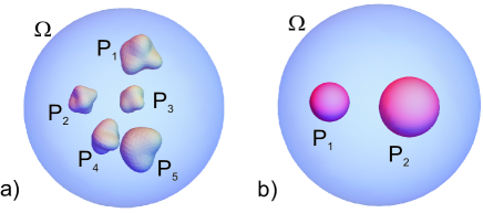
Figure 1: Geometric situation a) in the general case, and b) for the simplified model.

To show this result, it is first proved that there is no non-zero charge distribution in one region, that annihilates the signal of a charge distribution in another, topologically separated region. This is the content of the No-Mutual-Annihilator theorem in section  2.

From that the main theorem on unique source assignment in section 3 follows directly by the linearity of the von Neumann boundary value problem for the Poisson equation. Therefore, the main mathematical content is encapsulated in the two-region NMA theorem, that can be regarded as a far reaching generalization of a theorem of Gauss about separating the internal and external components of the geomagnetic field (Gauss, 1877; Backus et al., 1997). It essentially relies on the fact that harmonic functions are analytic and can be uniquely analytically continued on simply connected open sets (Axler et al., 2001, Theorem 1.27).

2 The No-Mutual-Annihilator theorem

Let $\Omega\subset\mathbb{R}^{3}$ be open and $\partial\Omega$ a nonempty, smooth compact manifold. For a set $G$ with $\overline{G}\subset\Omega$ the (Neumann) annihilator of $G$ in $\partial\Omega$ is defined as

$${\rm Ann}(G):=\left\{\rho\in L^{1}(G):{\rm supp}\,\rho\subset\mathring{G},\right.$$

$$\left.\exists\Phi\in C^{2}(\Omega)\cap C^{1}(\overline{\Omega}):\Delta\,\Phi=\rho{~{}~{}\rm and~{}~{}}\frac{\partial\Phi}{\partial n}=0{\rm~{}on~{}}\partial\Omega\right\}.$$

Physically, ${\rm Ann}(G)$ represents the vector space of all possible charge distributions inside the region $G$ which create no measurement signal on the boundary $\partial\Omega$. Because the measurement signal is the normal derivative of the potential field, the potential itself is only defined up to a globally constant summand, and in the following this constant is chosen such that the analytic continuation of $\Phi$ to $\mathbf{R}^{3}$ vanishes at infinity. The corresponding potentials are called zero-gauged.

$N$ pairwise disjoint compact sets $P_{1},\ldots,P_{N}$ with $P_{i}\subset\Omega$ have the no-mutual-annihilator (NMA) property if

$${\rm Ann}(\bigcup\limits_{i=1}^{N}P_{i})~{}=~{}\bigoplus\limits_{i=1}^{N}{\rm Ann}(P_{i}).$$

In the above equation the ”$\supset$” inclusion is always true, because any element of the vector space spanned by the annihilators of the $P_{i}$ is an annihilator of the union $\bigcup\limits_{i=1}^{N}P_{i}$. The other inclusion ”$\subset$” in the NMA property implies, that it is impossible to have a charge distribution $\rho$ within the region $\bigcup\limits_{i=1}^{N}P_{i}$ which generates a zero signal on the boundary, such that if the charge distribution is set to zero in some, but not all, of the $P_{i}$, the resulting boundary signal is not zero.

An example of two sets which do not have the NMA property are two nested balls $P_{1}=B(r)$ and $P_{2}=B(R)\backslash B(r)$ for $0<r<R$. A well-known annihilator in this case are constant non-zero charge distributions of opposite sign such that the integral over $B(R)$ is zero (Zhdanov, 2015). Setting the charge distribution in one of $P_{1},P_{2}$ to zero clearly generates a non-zero field on $\partial\Omega$.

Intuitively it appears plausible that two point charges inside a sphere, which lie far apart from each other, but close to the surface of the sphere do have the NMA property. At least if the charge distribution inside one of them has a non-zero total charge, then the other must have the opposite total charge to annihilate the field at large distance, but at small distance on the surface $\partial\Omega$ these charges cannot cancel each other.

It is also known that the annihilator sets ${\rm Ann}(G)$ for $\overline{G}\subset\Omega$ are large. For star-shaped $G$, any charge distribution $\rho\in L^{1}(G)$ which for all harmonic functions $h\in C^{2}(\Omega):\Delta\,h\,=\,0$ fulfills

$$\int\limits_{G}h(r)\,\rho(r)\,dV\,=\,0$$

generates no field on $\partial\Omega$, such that $\rho\in{\rm Ann}(G)$ (Zhdanov, 2015). This apparently bleak state of affairs with respect to unique-inversion results is emphasized by the fact that (Zhdanov, 2015) reports as the best result so far that if a gravity field is generated by a star-shaped body of constant density $\rho(r)=\rho_{0}$, the gravity inverse problem has a unique solution (Novikov, 1938).

It therefore may appear incredible that a far-reaching uniqueness result, as claimed above, is not in conflict with the known non-uniqueness results. We will now show that it is mathematically feasible. To make the proof easier to follow, it is first shown under relatively weak topological conditions that two disjoint regions have the NMA property. By induction this is then generalized to a finite number of $N$ regions. The essential property to avoid non-uniqueness of the inversion is that the complement of these finite regions is a simply connected region where analytical continuation is uniquely possible. Thereby uniqueness of the inversion is closely linked to uniqueness of analytical continuation.

Two-region NMA theorem.

Let $\Omega\subset\mathbf{R}^{3}$ be open and $\partial\Omega$ a smooth compact manifold and $P_{1},P_{2}\subset\Omega$ be disjoint compact sets, such that $\mathbb{R}^{3}\backslash P_{1}$, $\mathbb{R}^{3}\backslash P_{2}$, and $\mathbb{R}^{3}\backslash(P_{1}\cup P_{2})$ are simply connected then $P_{1}$ and $P_{2}$ have the No-Mutual-Annihilator property with respect to $\Omega$.

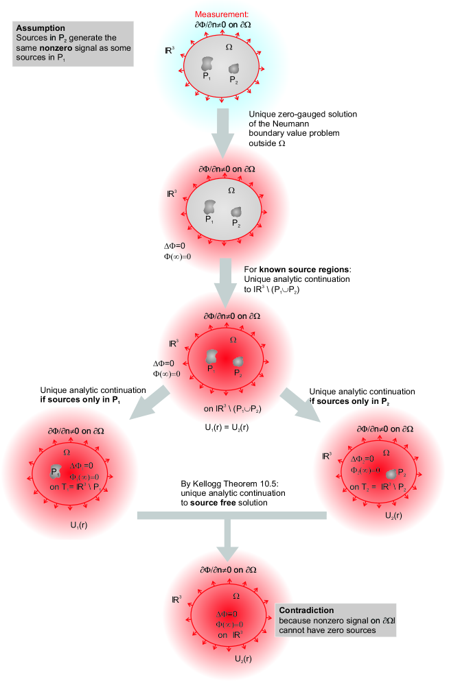
Figure 2: Overview of the proof of the two-region NMA theorem. The assumption that sources in region $P_{1}$ generate the same nonzero field on the surface $\partial\Omega$ as sources inside region $P_{2}$ leads to a contradiction if $T_{1}$ and $T_{2}$ are simply connected.

Proof.

We derive a contradiction from the assumption that there exists a mutual annihilator

$$\rho\in{\rm Ann}(P_{1}\cup P_{2})\backslash({\rm Ann}(P_{1})\oplus{\rm Ann}(P_{2})).$$

By definition, then there are two nonzero functions $\rho_{1},\rho_{2}\in L^{1}(\Omega)$ with ${\rm supp}\,\rho_{1}\subset P_{1}$, ${\rm supp}\,\rho_{2}\subset P_{2}$, such that

$$\rho=\rho_{1}-\rho_{2},$$

and the non-zero normal derivatives of their potentials $\frac{\partial\Phi_{1}}{\partial n},\frac{\partial\Phi_{2}}{\partial n}$ are identical on $\partial\Omega$. Now recall that the solution of the Neumann problem for harmonic functions is unique for zero-gauged potentials (Kellogg, 1929, Theorem 8.4), by which $\Phi_{1}=\Phi_{2}$ on $\mathbb{R}^{3}\backslash\Omega$, where a potential $U$ is called zero-gauged, if

$$\lim\limits_{||x||\to\infty}U(x)~{}=~{}0.$$

We now conjure up a bit of mathematical magic in form of Theorem 10.5 in (Kellogg, 1929) which essentially encapsulates Gauss theorem of separation of sources. By assumption, the sets $T_{1}:=\mathbb{R}^{3}\backslash P_{1}$ and $T_{2}:=\mathbb{R}^{3}\backslash P_{2}$ are simply connected and open and overlap on the simply connected set $\mathbb{R}^{3}\backslash(P_{1}\cup P_{2})$. By analytic continuation on the simply connected open sets $T_{1}$ and $T_{2}$ (Axler et al., 2001, Theorem 1.27) there is a unique harmonic function $U_{1}$ on $T_{1}$ with $U_{1}=\Phi_{1}$ on $\mathbb{R}^{3}\backslash\Omega$, and a unique $U_{2}$ on $T_{2}$ with $U_{2}=\Phi_{2}$ on $\mathbb{R}^{3}\backslash\Omega$. By (Kellogg, 1929, Theorem 10.5 ), there now also is a unique harmonic function $U$ on $\mathbb{R}^{3}$ with $U=U_{1}$ on $T_{1}$ and $U=U_{2}$ on $T_{2}$. This implies that $U$ solves the zero-gauged Neumann problem $\Delta U=0$ on $\mathbb{R}^{3}$ with boundary condition $\frac{\partial U}{\partial n}=\frac{\partial\Phi_{1}}{\partial n}$ on $\partial\Omega$. Because the unique zero-gauged potential with $\Delta U=0$ on $\mathbb{R}^{3}$ is $U=0$, it follows that $\rho_{1}=\rho_{2}=0$ which contradicts the assumption. ∎

Because the above proof is quite mathematical in nature, in the supplementary information the special case of a two-ball NMA theorem, in which $P_{1,2}$ are disjoint balls as in Fig. 1b, is proved by directly applying Gauss theorem of separation of sources. This may help to acquire a physical understanding of the strength and limitations of the result, and may also lend more credulity to the derivation above. In the next step the result of the two-region NMA theorem is extended to arbitrary numbers of regions by induction.

Corollary: General NMA theorem.

Let $\Omega\subset\mathbf{R}^{3}$ be open and $\partial\Omega$ a smooth compact manifold. For a natural number $N\geq 1$ let $P_{1},\ldots,P_{N}\subset\Omega$ be pairwise disjoint compact sets, such that $\mathbb{R}^{3}\backslash P_{k}$ and $\mathbb{R}^{3}\backslash\bigcup\limits_{i=1}^{k}P_{i}$ are simply connected for all $k=1,\ldots,N$. Then the $P_{i}$ have the No-Mutual-Annihilator property with respect to $\Omega$.

Proof.

For $N=1$ there is nothing to prove. Assume that $N>1$ and that the corollary is true for $N-1$. Define the sets $P_{1}^{\prime}=\bigcup\limits_{i=1}^{N-1}P_{i}$ and $P_{2}^{\prime}=P_{N}$. The assumptions on the $P_{k}$ imply that $P_{1}^{\prime}$ and $P_{2}^{\prime}$ fulfill the conditions to apply the two-region NMA theorem, whereby $P_{1}^{\prime}$ and $P_{2}^{\prime}$ have the No-Mutual-Annihilator property with respect to $\Omega$ which implies

$${\rm Ann}(\bigcup\limits_{i=1}^{N}P_{i})~{}=~{}{\rm Ann}(\bigcup\limits_{i=1}^{N-1}P_{i})\oplus{\rm Ann}(P_{N}).$$

Because the corollary is true for $N-1$ and $P_{1},\ldots,P_{N-1}$ fulfill the conditions for its application we have by induction

$${\rm Ann}(\bigcup\limits_{i=1}^{N-1}P_{i})~{}=~{}\bigoplus\limits_{i=1}^{N-1}{\rm Ann}(P_{i}).$$

Substituting this in the above equation proves the corollary. ∎

3 Unique source assignment

The previous two theorems provide all prerequisites to formulate the main result of this article:

Unique source assignment theorem.

Let $\Omega\subset\mathbb{R}^{3}$ be open, simply connected, and $\partial\Omega$ a smooth compact manifold. Assume that $P_{1},\ldots,P_{N}\subset\Omega$ are pairwise disjoint compact sets such that $\mathbb{R}^{3}\backslash P_{k}$ and $\mathbb{R}^{3}\backslash\bigcup\limits_{i=1}^{k}P_{i}$ are simply connected for all $k=1,\ldots,N$. If the sources of the zero-gauged potential $\Phi$ have compact support on $\bigcup\limits_{k=1}^{N}P_{k}$, then $\frac{\partial\Phi}{\partial n}$ on $\partial\Omega$ uniquely determines zero-gauged potentials $\Phi_{1},\ldots,\Phi_{N}$, such that $\Phi_{i}$ is harmonic on $\mathbb{R}^{3}\backslash\bigcup\limits_{k\neq i}P_{k}$, which implies that it has no sources outside $P_{i}$, and

$$\frac{\partial\Phi}{\partial n}~{}=~{}\sum\limits_{i=1}^{N}\frac{\partial\Phi_{i}}{\partial n}~{}~{}{\rm on}~{}~{}\partial\Omega.$$

Proof.

Because the source of $\Phi$ is a charge distribution $\rho$ in $\bigcup\limits_{k=1}^{N}P_{k}$ there exist zero-gauged harmonic potentials $\Phi_{1},\ldots,\Phi_{N}$ with the required properties, namely those generated by the local charge distributions $\rho_{k}=\rho|_{P_{k}}$.

Uniqueness is now shown by the general NMA theorem. Take any charge distribution $\rho^{\prime}$ in $\bigcup\limits_{k=1}^{N}P_{k}$ with zero-gauged potentials $\Psi_{1},\ldots,\Psi_{N}$, such that $\Psi_{i}$ is harmonic on $\mathbb{R}^{3}\backslash\bigcup\limits_{k\neq i}P_{k}$ and

$$\frac{\partial\Phi}{\partial n}~{}=~{}\sum\limits_{i=1}^{N}\frac{\partial\Psi_{i}}{\partial n}~{}~{}{\rm on}~{}~{}\partial\Omega.$$

Then define $\Gamma_{i}=\Phi_{i}-\Psi_{i}$ such that $\Gamma$ with

$$\Gamma:=\sum\limits_{i=1}^{N}\Gamma_{i}~{}=~{}0~{}~{}{\rm on}~{}~{}\mathbb{R}^{3}\backslash\Omega,~{}~{}{\rm and}~{}~{}\frac{\partial\Gamma}{\partial n}~{}=~{}0~{}~{}{\rm on}~{}~{}\partial\Omega,$$

is the zero-gauged potential from the source distribution $\rho-\rho^{\prime}$, which thereby is a member of

$${\rm Ann}(\bigcup\limits_{i=1}^{N}P_{i})~{}=~{}\bigoplus\limits_{i=1}^{N}{\rm Ann}(P_{i}).$$

The equality is due to the general NMA theorem and its right hand side implies that $\Gamma_{i}~{}=~{}0$, or $\Phi_{i}=\Psi_{i}$ for $i=1,\ldots,N$. Thus the zero-gauged $\Phi_{i}$ are uniquely determined by $\frac{\partial\Phi}{\partial n}$ on $\partial\Omega$. ∎

3.1 Unique source assignment is well-posed

When denoting by $H_{0}(\mathbb{R}^{3}\backslash P)$ the space of harmonic, zero-gauged functions outside a compact region $P$, the linear operator for solving the inverse problem

$$A:H_{0}(\mathbb{R}^{3}\backslash(P_{1}\cup P_{2}))\to H_{0}(\mathbb{R}^{3}\backslash P_{1}),~{}~{}\Phi\mapsto~{}\Phi_{1}$$

has the nullspace $H_{0}(\mathbb{R}^{3}\backslash P_{2})$ which is closed in $H_{0}(\mathbb{R}^{3}\backslash(P_{1}\cup P_{2}))$, whereby $A$ is continuous (Rudin, 1991, theorem 1.18). Accordingly the source assignment problem a) has a solution, b) this solution is unique, and c) the operator that maps the measurement to the solution is continuous, which by Hadamard’s definition (Zhdanov, 2015) implies that the inversion is a well-posed problem. In case of sufficiently dense data and low signal-to-noise ratio the inverse problem therefore can be expected to be solvable in a stable and robust way. As with any inverse problem, the numerical inversion can still be ill-conditioned, for example in cases where the the discretization is too coarse or the signal-to-noise ratio is low.

4 Consequences

This new theorem provides a clear and astoundingly general condition for when it is theoretically possible to uniquely assign potential field signals to source regions. To give a intuitive argument why this kind of theorem can exist, consider the simple case when $\Omega$ and all $P_{k}$ are balls. The theorem now guarantees that from the spherical harmonic expansion of the field on $\partial\Omega$ all individual spherical harmonic expansions on the $\partial P_{k}$ are uniquely determined. Thus the coefficients of one countably infinite basis of an harmonic function space uniquely define $N$ countably infinite coefficient sets on $N$ infinite bases, which is no contradiction in analogy to the Hilbert-hotel paradox (Hilbert, 1924/1925).

Unique source assignment is significant in geophysics for gravimetric, or aeromagnetic interpretation, when combined with tomographic methods like seismic imaging. It also lies the foundation for reading three-dimensional magnetic storage media. In rock-magnetism, after the pioneering work of Egli and Heller (2000), different magnetic surface scanning techniques are increasingly used to infer magnetization sources and magnetization structure inside rocks (e.g. Uehara and Nakamura, 2007; Hankard et al., 2009; Usui et al., 2012; Lima et al., 2013; Glenn et al., 2017). In this context, the unique source-assignment theorem enables paleomagnetic reconstruction from natural particle ensembles (de Groot et al., 2018), because it establishes that individual dipole moments from a large number of magnetic particles in a non-magnetic matrix that are localized by density tomography (micro-CT) can be uniquely recovered from surface magnetic field measurements. In de Groot et al. (2018) uniqueness of dipole reconstruction is individually certified by showing that for some specific set of $K$ magnetic particles found by density tomography one can find $3K$ surface measurements such that the a $3K\times 3K$-matrix of the forward calculation is invertible. This proves that only a unique set of dipoles can explain the measurement. The result proven here is much more general in that it asserts, that no two different sets of multipole expansions originating from the particles can lead to the same surface signal. The induction proof of the unique source assignment theorem even indicates a divide-and-conquer type strategy for algorithmic implementation of an inverse reconstruction.

When scanning a sample in its natural-remanent magnetization state, and again after applying standard paleomagnetic stepwise demagnetization procedures, the resultant demagnetization data set can be studied on an individual particle level to identify stable and unaltered remanence carriers. By selecting only optimally preserved and stable remanence carriers from a large collection of measured particles, reliable statistical average paleomagnetic directions or NRM intensities can be calculated for terrestrial or extraterrestrial rocks that due to unresolvable noise currently could not be used as recorders of their magnetic history.

Further potential application areas of unique source assignment theorems are for example inversion problems in EEG (electroencephalography), MEG (magnetoencephalography), or ECG(electrocardiography), where it might enable to uniquely assign externally measured potential field signals to previously determined brain or heart regions (Baillet et al., 2001; Michel et al., 2004; Grech et al., 2008; Michel and Murray, 2012; Huster et al., 2012). Empirical inversion techniques that now use numerical and statistical approaches to assess the reliability of their results (Friston et al., 2008; Castano-Candamil et al., 2015) may profit from unique source assignment to prior known regions.

What essentially remains impossible is to assign signals to source regions which lie inside other source regions, like the nested balls described in section 2. These cases are excluded, because they do not fulfill the condition of simple connectivity of $\mathbb{R}^{3}\backslash P_{k}$ for all $k$, which makes analytic continuation impossible. The fact that this appears to be the only obstruction to unique reconstruction provides a new incentive and direction to study potential field measurement techniques in combination with a priori source localization to recover a maximum of information about the spherical harmonic expansion of the individual source regions.

Supplementary information

Kelloggs theorem 10.5.

If $T_{1}$ and $T_{2}$ are two domains with common points, and if $U_{1}$ is harmonic in $T_{1}$ and $U_{2}$ in $T_{2}$, these functions coinciding at the common points of $T_{1}$ and $T_{2}$, then they define a single function, harmonic in the domain $T$ consisting of all points of $T_{1}$ and $T_{2}$.[Kellogg, 1929]

Two-ball NMA theorem.

Let $\Omega\subset\mathbf{R}^{3}$ be open and $\partial\Omega$ a smooth compact manifold and $P_{1},P_{2}\subset\Omega$ be disjoint balls, then $P_{1}$ and $P_{2}$ have the No-Mutual-Annihilator property with respect to $\Omega$.

Proof.

If there exists a mutual annihilator

$$\rho\in{\rm Ann}(P_{1}\cup P_{2})\backslash({\rm Ann}(P_{1})\oplus{\rm Ann}(P_{2})),$$

then there are two nonzero functions $\rho_{1},\rho_{2}\in L_{1}(\Omega)$ with ${\rm supp}\,\rho_{1}\subset P_{1}$, ${\rm supp}\,\rho_{2}\subset P_{2}$, and $\rho=\rho_{1}-\rho_{2}$, such that the non-zero normal derivatives of their potentials $\frac{\partial\Phi_{1}}{\partial n},\frac{\partial\Phi_{2}}{\partial n}$ are identical on $\partial\Omega$. Because the solution of the Neumann problem for zero-gauged harmonic functions is unique, $\Phi_{1}=\Phi_{2}$ on $\mathbf{R}^{3}\backslash\Omega$. Because $P_{1},P_{2}$ are disjoint $\mathbb{R}^{3}\backslash\overline{P_{1}\cup P_{2}}$ is an open simply connected set and the harmonic functions $\Phi_{1},\Phi_{2}$ are defined on $\mathbb{R}^{3}\backslash\overline{P_{1}\cup P_{2}}$, and equal on the nonempty open set $\mathbb{R}^{3}\backslash\overline{\Omega}$. Because every harmonic function is analytic, this implies $\Phi_{1}~{}=~{}\Phi_{2}$ on $\mathbb{R}^{3}\backslash\overline{P_{1}\cup P_{2}}$[Axler et al., 2001, theorem 1.27]
For the potential $\Phi_{1}$ all sources lie inside $P_{1}$ and $\frac{\partial\Phi_{1}}{\partial n}$ on $\partial P_{2}$ is uniquely defined. By Gauss theorem [Gauss, 1877, Backus et al., 1997], the spherical harmonic expansion of $\Phi_{1}$ on $\partial P_{2}$ is uniquely defined from $\frac{\partial\Phi_{1}}{\partial n}$ on $\partial P_{2}$ and thus only contains terms related to external sources, because ${\rm supp}\,\rho_{1}$ is outside of $\partial P_{2}$. On the other hand $\frac{\partial\Phi_{1}}{\partial n}~{}=~{}\frac{\partial\Phi_{2}}{\partial n}$ on $\partial P_{2}$, and the spherical harmonic expansion of $\Phi_{2}$ on $\partial P_{2}$ has only Gauss coefficients from inner sources, because ${\rm supp}\,\rho_{2}$ is inside of $\partial\Omega_{2}$. Because a non-zero potential cannot at the same time have only inner sources and only outer sources, a mutual annihilator cannot exist. ∎

References

- Axler et al. [2001] S. Axler, P. Bourdon, and W. Ramey. Harmonic Function Theory. Springer, New York, 2nd edition, 2001.
- Backus et al. [1997] P. Backus, R. Parker, and C. Constable. Foundations of Geomagnetism. Cambridge University Press, Cambridge, 1997.
- Baillet et al. [2001] S. Baillet, J. C. Mosher, and R. M. Leahy. Electromagnetic brain mapping. Ieee Signal Processing Magazine, 18(6):14–30, 2001.
- Baratchart et al. [2013] L. Baratchart, D. P. Hardin, E. A. Lima, E. B. Saff, and B. P. Weiss. Characterizing kernels of operators related to thin-plate magnetizations via generalizations of Hodge decompositions. Inverse Problems, 29:015004 (29 pp), 2013.
- Castano-Candamil et al. [2015] S. Castano-Candamil, J. Hohne, J. D. Martinez-Vargas, X. W. An, G. Castellanos-Dominguez, and S. Haufe. Solving the EEG inverse problem based on space-time-frequency structured sparsity constraints. Neuroimage, 118:598–612, 2015.
- de Groot et al. [2018] L. V. de Groot, K. Fabian, A. Béguin, P. Reith, A. Barnhoorn, and H. Hilgenkamp. Determining individual particle magnetizations in assemblages of micro-grains. Geophys. Res. Lett., 45, 2018. doi: 10.1002/2017GL076634.
- Egli and Heller [2000] R. Egli and F. Heller. High-resolution imaging using a high-T-c superconducting quantum interference device (SQUID) magnetometer. Journal of Geophysical Research-Solid Earth, 105:25709–25727, 2000.
- Friston et al. [2008] K. J. Friston, L. Harrison, J. Daunizeau, S. Kiebel, C. Phillips, N. Trujillo-Barreto, R. Henson, G. Flandin, and J. Mattout. Multiple sparse priors for the M/EEG inverse problem. Neuroimage, 39(3):1104–1120, 2008.
- Gauss [1877] C. F. Gauss. Werke, Fünfter Band. Springer, Berlin, Heidelberg, 1877.
- Glenn et al. [2017] D. R. Glenn, R. R. Fu, P. Kehayias, D. Le Sage, E. A. Lima, B. P. Weiss, and R. L. Walsworth. Micrometer-scale magnetic imaging of geological samples using a quantum diamond microscope. Geochemistry Geophysics Geosystems, 18(8):3254–3267, 2017.
- Grech et al. [2008] R. Grech, T. Cassar, J. Muscat, K. P. Camilleri, S. G. Fabri, M. Zervakis, P. Xanthopoulos, V. Sakkalis, and B. Vanrumste. Review on solving the inverse problem in EEG source analysis. Journal of Neuroengineering and Rehabilitation, 5, 2008.
- Hankard et al. [2009] F. Hankard, J. Gattacceca, C. Fermon, M. Pannetier-Lecoeur, B. Langlais, Y. Quesnel, P. Rochette, and S. A. McEnroe. Magnetic field microscopy of rock samples using a giant magnetoresistance-based scanning magnetometer. Geochemistry Geophysics Geosystems, 10, 2009.
- Hilbert [1924/1925] David Hilbert. Über das Unendliche. Vorlesung, 1924/1925.
- Huster et al. [2012] R. J. Huster, S. Debener, T. Eichele, and C. S. Herrmann. Methods for simultaneous EEG-fMRI: An introductory review. Journal of Neuroscience, 32(18):6053–6060, 2012.
- Kellogg [1929] O. D. Kellogg. Foundations of Potential Theory. Springer, New York, 1929.
- Lima et al. [2013] E. A. Lima, B. P. Weiss, L. Baratchart, D. P. Hardin, and E. B. Saff. Fast inversion of magnetic field maps of unidirectional planar geological magnetization. Journal of Geophysical Research-Solid Earth, 118(6):2723–2752, 2013.
- Michel and Murray [2012] C. M. Michel and M. M. Murray. Towards the utilization of EEG as a brain imaging tool. Neuroimage, 61(2):371–385, 2012.
- Michel et al. [2004] C. M. Michel, M. M. Murray, G. Lantz, S. Gonzalez, L. Spinelli, and R. G. de Peralta. EEG source imaging. Clinical Neurophysiology, 115(10):2195–2222, 2004.
- Novikov [1938] P. S. Novikov. Sur le problème inverse du potential. Dokl. Acad. Sci. URSS, 18:165–168, 1938.
- Rudin [1991] W. Rudin. Functional Analysis. McGraw-Hill, New York, 2nd edition, 1991.
- Uehara and Nakamura [2007] M. Uehara and N. Nakamura. Scanning magnetic microscope system utilizing a magneto-impedance sensor for a nondestructive diagnostic tool of geological samples. Review of Scientific Instruments, 78(4), 2007.
- Usui et al. [2012] Y. Usui, M. Uehara, and K. Okuno. A rapid inversion and resolution analysis of magnetic microscope data by the subtractive optimally localized averages method. Computers & Geosciences, 38(1):145–155, 2012.
- Zhdanov [2015] Michael S. Zhdanov. Inverse Theory and Applications in Geophysics. Elsevier, Amsterdam, 2nd edition, 2015.