“Zero-Shot” Super-Resolution using Deep Internal Learning

Abstract

Deep Learning has led to a dramatic leap in Super-Resolution (SR) performance in the past few years. However, being supervised, these SR methods are restricted to specific training data, where the acquisition of the low-resolution (LR) images from their high-resolution (HR) counterparts is predetermined (e.g., bicubic downscaling), without any distracting artifacts (e.g., sensor noise, image compression, non-ideal PSF, etc). Real LR images, however, rarely obey these restrictions, resulting in poor SR results by SotA (State of the Art) methods. In this paper we introduce “Zero-Shot” SR, which exploits the power of Deep Learning, but does not rely on prior training. We exploit the internal recurrence of information inside a single image, and train a small image-specific CNN at test time, on examples extracted solely from the input image itself. As such, it can adapt itself to different settings per image. This allows to perform SR of real old photos, noisy images, biological data, and other images where the acquisition process is unknown or non-ideal. On such images, our method outperforms SotA CNN-based SR methods, as well as previous unsupervised SR methods. To the best of our knowledge, this is the first unsupervised CNN-based SR method.

(a) Historic image: Check-point Charlie (end of World-War II) – $SR\times 2$
	ZSSR (ours)
	EDSR [12]

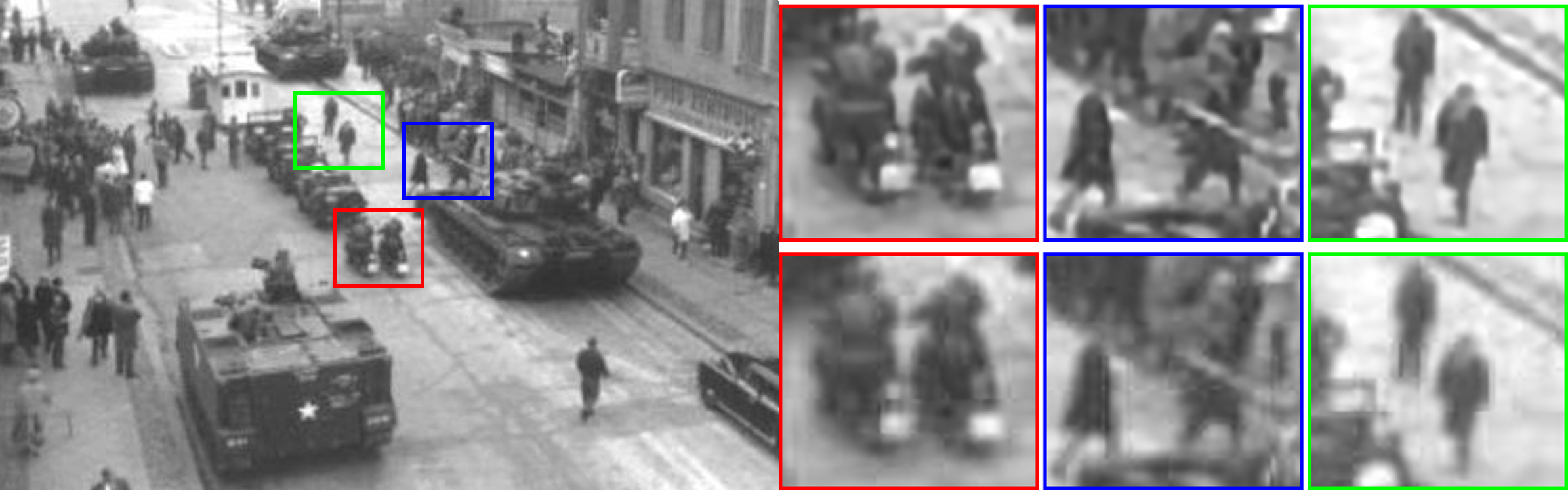
(a)

(b) iPhone image – $SR\times 3$	(c) Historic image: JFK funeral – $SR\times 2$
	EDSR [12]          ZSSR (ours)
	(d) Outdoor image downloaded from the Internet – $SR\times 2$
EDSR [12]          ZSSR (ours)	EDSR [12]                                ZSSR (ours)

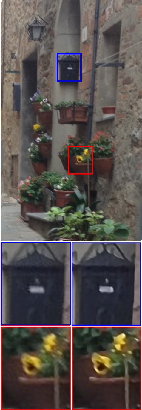
(b)

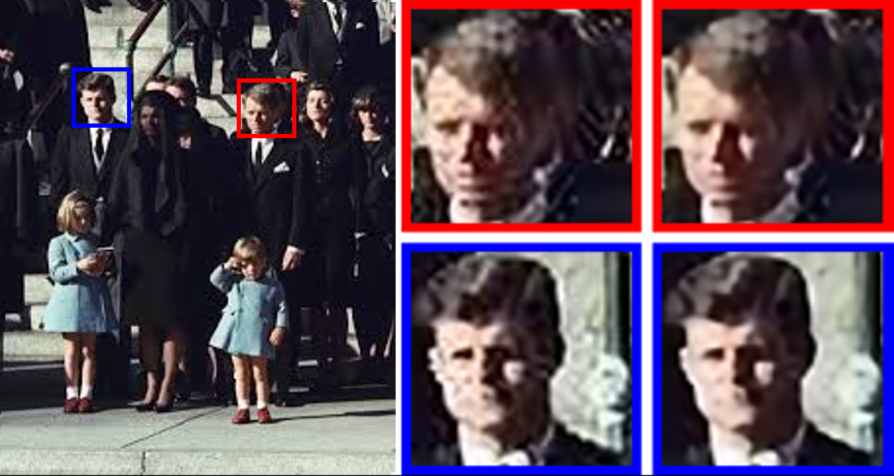
(c)

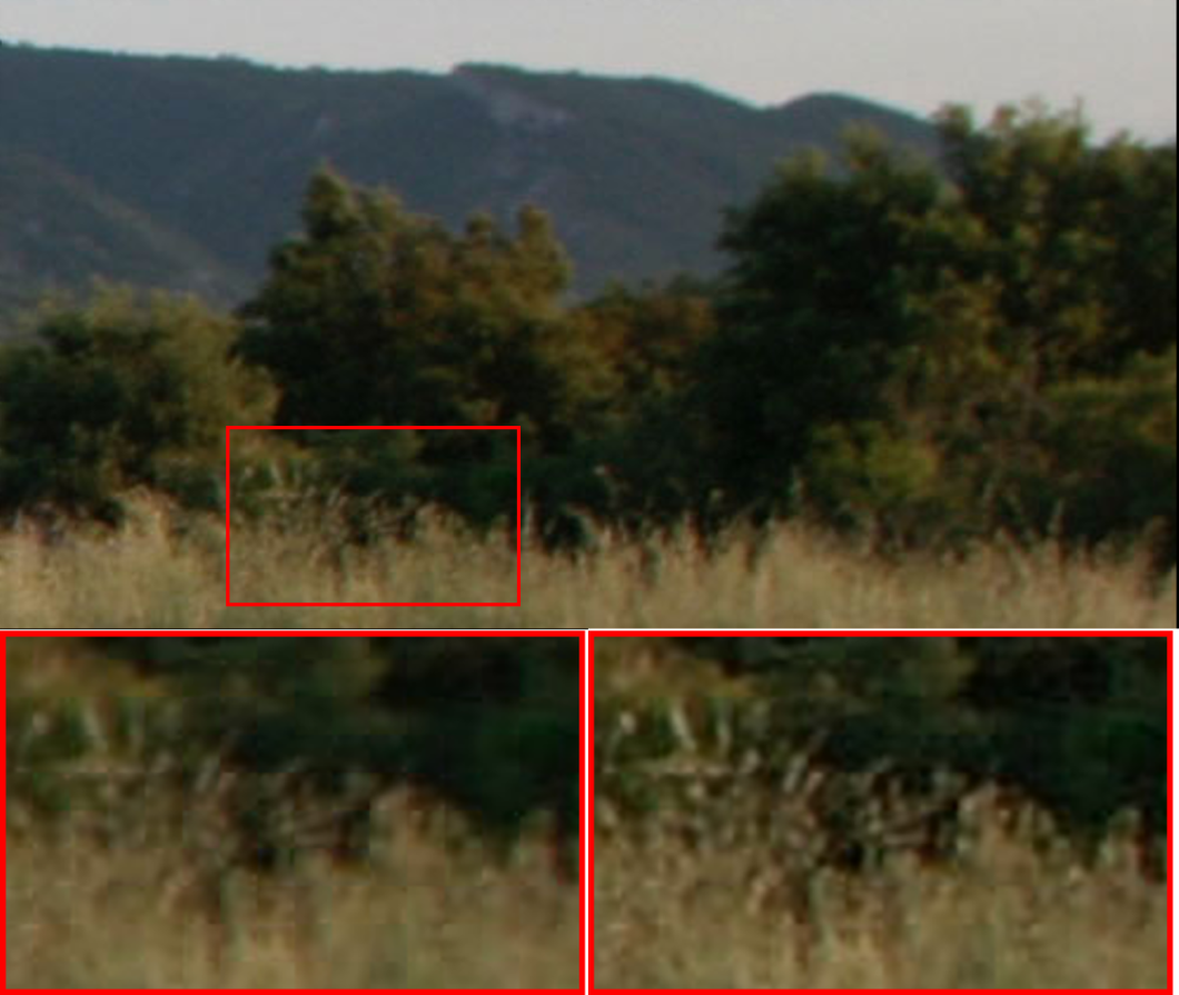
(d)

Figure 1: SR of real images (unknown LR acquisition process). Real-world images rarely obey the ‘ideal conditions’ assumed by supervised SR methods. For example, old historic photos (a,c), images taken by smartphones (b), random images on the Internet (d), etc. Since ZSSR trains at test time on examples extracted from the test image, it is better at performing SR ‘In-the-Wild’ (i.e., in unconstrained and unknown settings). Full sized images can be found on our project website.

(a) SR under aliasing:

	Ground truth	EDSR+ [12]	ZSSR (ours)
	(PSNR /SSIM)	( 21.64 / 0.6641)	(25.02 / 0.7658)

(b) SR under unknown non-ideal downscaling kernel:

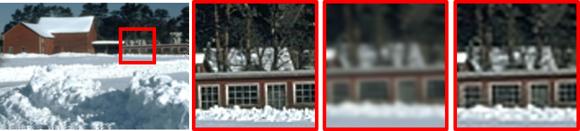
	Ground truth	EDSR+ [12]	ZSSR (ours)
	(PSNR /SSIM)	(24.44 / 0.7006)	(27.62 / 0.8367)

Figure 2: SR of ‘non-ideal’ LR images – a controlled experiment. (a) LR image generated with aliasing (donwscaling kernel is a delta function). (b) LR image generated with a non-ideal downscaling kernel. The unknown image-specific kernel is estimated directly from the LR test image using [14], and fed into our image-specific CNN as the downscaling kernel (note that externally-trained networks cannot make use of such image-specific information at test-time). Full sized images can be found on our project website. Quantitative evaluation on hundreds of ‘non-ideal’ LR images can be found in Sec. 4.2.

1 Introduction

Super-Resolution (SR) from a single image has recently received a huge boost in performance using Deep-Learning based methods [3, 9, 8, 11, 12]. The recent SotA (State of the Art) method [12] exceeds previous non-Deep SR methods (supervised [21] or unsupervised [4, 5, 6]) by a few dBs – a huge margin! This boost in performance was obtained with very deep and well engineered CNNs, which were trained exhaustively on external databases, for lengthy periods of time (days or weeks). However, while these externally supervised methods perform extremely well on data satisfying the conditions they were trained on, their performance deteriorates significantly once these conditions are not satisfied.

For example, SR CNNs are typically trained on high-quality natural images, from which the low-resolution (LR) images were generated with a specific predefined downscaling kernel (usually a Bicubic kernel with antialiasing – MATLAB’s default imresize command), without any distracting artifacts (sensor noise, non-ideal PSF, image compression, etc.), and for a predefined SR scaling-factor (usually $\times 2$, $\times 3$ or $\times 4$; assumed equal in both dimensions). Fig. 2 shows what happens when these conditions are not satisfied, e.g., when the LR image is generated with a non-ideal (non-bicubic) downscaling kernel, or contains aliasing effects, or simply contains sensor noise or compression artifacts. Fig. 1 further shows that these are not contrived cases, but rather occur often when dealing with real LR images – images downloaded from the internet, images taken by an iPhone, old historic images, etc. In those ‘non-ideal’ cases, SotA SR methods often produce poor results.

In this paper we introduce “Zero-Shot” SR (ZSSR), which exploits the power of Deep Learning, without relying on any prior image examples or prior training. We exploit the internal recurrence of information within a single image and train a small image-specific CNN at test time, on examples extracted solely from the LR input image itself (i.e., internal self-supervision). As such, the CNN can be adapted to different settings per image. This allows to perform SR on real images where the acquisition process is unknown and non-ideal (see example results in Figs. 1 and 2). On ‘non-ideal’ images, our method outperforms externally-trained SotA SR methods by a large margin.

The recurrence of small pieces of information (e.g., small image patches) across scales of a single image, was shown to be a very strong property of natural images [4, 23]. This formed the basis for many unsupervised image enhancement methods, including unsupervised SR [4, 5, 6], Blind-SR [14] (when the downscaling kernel is unknown), Blind-Deblurring [15, 1], Blind-Dehazing [2], and more. While such unsupervised methods can exploit image-specific information (hence are less subject to the above-mentioned supervised restrictions), they typically rely on simple Eucledian similarity of small image patches, of predefined size (typically $5\times 5$), using K-nearest-neighbours search. As such, they do not generalize well to patches that do not exist in the LR image, nor to new implicitly learned similarity measures, nor can they adapt to non-uniform sizes of repeating structures inside the image.

Our image-specific CNN leverages on the power of the cross-scale internal recurrence of image-specific information, without being restricted by the above-mentioned limitations of patch-based methods. We train a CNN to infer complex image-specific HR-LR relations from the LR image and its downscaled versions (self-supervision). We then apply those learned relations on the LR input image to produce the HR output. This outperforms unsupervised patch-based SR by a large margin.

Since the visual entropy inside a single image is much smaller than in a general external collection of images [23], a small and simple CNN suffices for this image-specific task. Hence, even though our network is trained at test time, its train+test runtime is comparable to the test runtime of SotA supervised CNNs. Interestingly, our image-specific CNN produces impressive results (although not SotA) on the ‘ideal’ benchmark datasets used by the SotA supervised methods (even though our CNN is small and has not been pretrained), and surpasses SotA supervised SR by a large margin on ‘non-ideal’ images. We provide both visual and empirical evidence of these statements.

The term “Zero-Shot” used here, is borrowed from the domains of recognition/classification. Note however, that unlike these approaches for Zero-Shot Learning [22] or One-shot Learning [18], our approach does not require any side information/attributes or any additional images. We may only have a single test image at hand, one of a kind, and nothing else. Nevertheless, when additional information is available and provided (e.g., the downscaling kernel can be estimated directly from the test image using [14]), our image-specific CNN can make good use of this at test time, to further improve the results.

Our contributions are therefore several-fold:
(i) To our best knowledge, this is the first unsupervised CNN-based SR method.
(ii) It can handle non-ideal imaging conditions, and a wide variety of images and data types (even if encountered for the first time).
(iii) It does not require pretraining and can be run with modest amounts of computational resources.
(iv) It can be applied for SR to any size and theoretically also with any aspect-ratio.
(v) It can be adapted to known as well as unknown imaging conditions (at test time).
(v) It provides SotA SR results on images taken with ‘non-ideal’ conditions, and competitive results on ‘ideal’ conditions for which SotA supervised methods were trained on.

2 The Power of Internal Image Statistics

Fundamental to our approach is the fact that natural images have strong internal data repetition. For example, small image patches (e.g., $5$$\times$$5$, $7$$\times$$7$) were shown to repeat many times inside a single image, both within the same scale, as well as across different image scales. This observation was empirically verified by [4, 23] using hundreds of natural images, and was shown to be true for almost any small patch in almost any natural image.

Fig. 3 shows an example of a simple single-image SR based on internal patch recurrence (courtesy of [4]). Note that it is able to recover the tiny handrails in the tiny balconies, since evidence to their existence is found elsewhere inside this image, in one of the larger balconies. In fact, the only evidence to the existence of these tiny handrails exists internally, inside this image, at a different location and different scale. It cannot be found in any external database of examples, no matter how large this dataset is! As can be seen, SotA SR methods fail to recover this image-specific information when relying on externally trained images. While the strong internal predictive-power is exemplified here using a ‘fractal-like’ image, the internal predictive-power was analyzed and shown to be strong for almost any natural image [4].

In fact, it was empirically shown by [23] that the internal entropy of patches inside a single image is much smaller than the external entropy of patches in a general collection of natural images. This further gave rise to the observation that internal image statistics often provides stronger predictive-power than external statistics obtained from a general image collection. This preference was further shown to be particularly strong under growing uncertainty and image degradations (see [23, 16] for details).

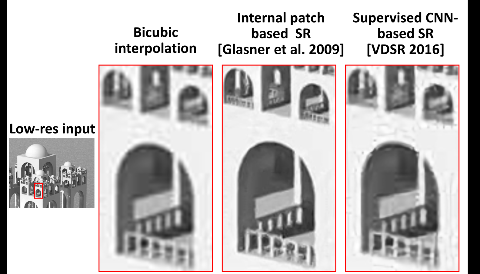
Figure 3: Internal predictive power of image-specific information. Simple unsupervised internal-SR [4] is able to reconstruct the tiny handrail in the tiny balconies, whereas externally-trained SotA SR methods fail to do so. Evidence to the existence of those tiny handrails exists only internally, inside this image, at a different location and scale (in one of the larger balconies). Such evidence is not found in any external database of images (no matter how large it is).

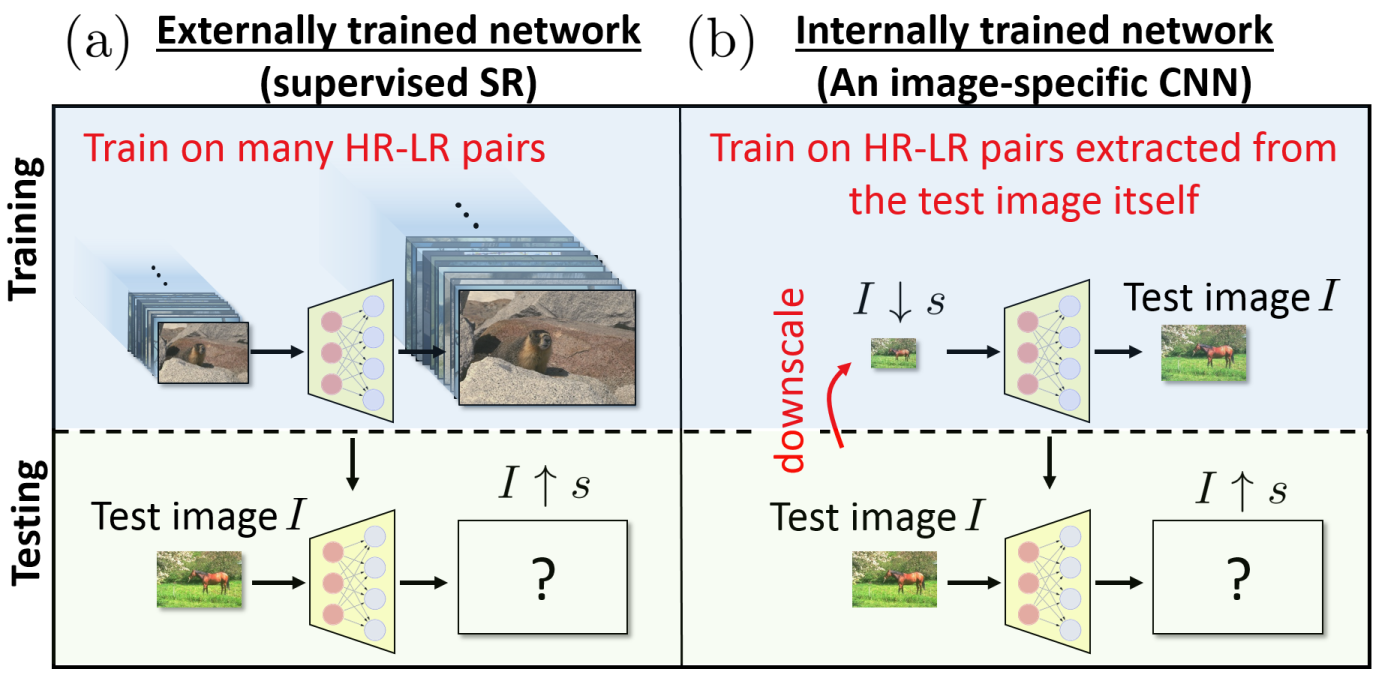
Figure 4: Image-Specific CNN – “Zero-Shot” SR.  (a) Externally-supervised SR CNNs are pre-trained on large external databases of images. The resulting very deep network is then applied to the test image $I$.  (b) Our proposed method (ZSSR): a small image-specific CNN is trained on examples extracted internally, from the test image itself. It learns how to recover the test image $I$ from its coarser resolutions. The resulting self-supervised network is then applied to the LR image $I$ to produce its HR output.

3 Image-Specific CNN

Our image-specific CNN combines the predictive power and low entropy of internal image-specific information, with the generalization capabilities of Deep-Learning. Given a test image $I$, with no external examples available to train on, we construct an Image-Specific CNN tailored to solve the SR task for this specific image. We train our CNN on examples extracted from the test image itself. Such examples are obtained by downscaling the LR image $I$, to generate a lower-resolution version of itself, $I\downarrow s$ (where $s$ is the desired SR scale factor). We use a relatively light CNN, and train it to reconstruct the test image $I$ from its lower-resolution version $I\downarrow s$ (top part of Fig. 4(b)). We then apply the resulting trained CNN to the test image $I$, now using $I$ as the LR input to the network, in order to construct the desired HR output $I\uparrow s$ (bottom of Fig. 4(b)). Note that the trained CNN is fully convolutional, hence can be applied to images of different sizes.

Since our “training set” consists of one instance only (the test image), we employ data augmentation on $I$ to extract more LR-HR example-pairs to train on. The augmentation is done by downscaling the test image $I$ to many smaller versions of itself ($I=I_{0},I_{1},I_{2},...,I_{n}$). These play the role of the HR supervision and are called “HR fathers”. Each of the HR fathers is then downscaled by the desired SR scale-factor $s$ to obtain the “LR sons”, which form the input training instances. The resulting training set consists of many image-specific LR-HR example pairs. The network can then stochastically train over these pairs.

We further enrich the training set by transforming each LR-HR pair using 4 rotations ($0^{\circ},90^{\circ},180^{\circ},270^{\circ}$) and their mirror reflections in the vertical and horizontal directions. This adds $\times 8$ more image-specific training examples.

For the sake of robustness, as well as to allow large SR scale factors $s$ even from very small LR images, the SR is performed gradually [4, 20]. Our algorithm is applied for several intermediate scale-factors ($s_{1},s_{2},...,s_{m}=s$). At each intemediate scale $s_{i}$, we add the generated SR image HR_i and its downscaled/rotated versions to our gradually growing training-set, as new HR fathers. We downscale those (as well as the previous smaller ‘HR examples’) by the next gradual scale factor $s_{i+1}$, to generate the new LR-HR training example pairs. This is repeated until reaching the full desired resolution increase $s$.

3.1 Architecture & Optimization

Supervised CNNs, which train on a large and diverse external collection of LR-HR image examples, must capture in their learned weights the large diversity of all possible LR-HR relations. As such, these networks tend to be extremely deep and very complex. In contrast, the diversity of the LR-HR relations within a single image is significantly smaller, hence can be encoded by a much smaller and simpler image-specific network.

We use a simple, fully convolutional network, with 8 hidden layers, each has 64 channels. We use ReLU activations on each layer. The network input is interpolated to the output size. As done in previous CNN-based SR methods [9, 8, 3], we only learn the residual between the interpolated LR and its HR parent. We use $L_{1}$ loss with ADAM optimizer [10]. We start with a learning rate of 0.001. We periodically take a linear fit of the reconstruction error and if the standard deviation is greater by a factor than the slope of the linear fit we divide the learning rate by 10. We stop when we get to a learning rate of $10^{-6}$.

To accelerate the training stage and make the runtime independent of the size of the test image $I$, at each iteration we take a random crop of fixed size from a randomly-selected father-son example pair. The crop is typically $128$$\times$$128$ (unless the sampled image-pair is smaller). The probability of sampling a LR-HR example pair at each training iteration is set to be non-uniform and proportional to the size of the HR-father. The closer the size-ratio (between the HR-father and the test image $I$) is to $1$, the higher its probability to be sampled. This reflects the higher reliability of non-synthesized HR examples over synthesize ones.

Lastly, we use a method similar to the geometric self-ensemble proposed in [12] (which generates 8 different outputs for the 8 rotations+flips of the test image $I$, and then combines them). We take the median of these 8 outputs rather than their mean. We further combine it with the back-projection technique of [7, 4], so that each of the 8 output images undergoes several iterations of back-projection and finally the median image is corrected by back-projection as well.

Runtime: Although training is done at test time, the average runtime per image is $54~{}sec$ for a single increase in SR scale-factor (on a Tesla K-80 GPU). This runtime is independent of the image size or the relative SR scale-factor $s$ (this is a result of the equally sized random crops used in training; the final test runtime is negligible with respect to training iterations). Nevertheless, better SR results are obtained when using a gradual increase in resolution. For example, a gradual increase using 6 intermediate scale-factors typically improves the PSNR by $\sim$$0.2{dB}$, but increases the runtime to $\sim$$5min$ per image. There is therefore a tradeoff between runtime and the output quality, which is up to the user to choose. Most of the results reported in this paper were produced using 6 intermediate scale-factors.

For comparison, the test-time of the leading EDSR+ [12] (on the same platform) is $\sim$$20~{}sec$ for SR$\times 2$ on a $200$$\times$$200$ image. However, EDSR’s run time grows quadratically with the image size, and reaches $5min$ for an $800\times 800$ image. Beyond that size, our network is faster than EDSR+.

3.2 Adapting to the Test Image

When the acquisition parameters of the LR images from their HR ones are fixed for all images (e.g., same downscaling kernel, high-quality imaging conditions), current supervised SR methods achieve an incredible performance [19]. In practice, however, the acquisition process tends to change from image to image, since cameras/sensors differ (e.g., different lens types and PSFs), as well as the individual imaging conditions (e.g., subtle involuntary camera shake when taking the photo, poor visibility conditions, etc). This results in different downscaling kernels, different noise characteristics, various compression artifacts, etc. One could not practically train for all possible image acquisition configurations/settings. Moreover, a single supervised CNN is unlikely to perform well for all possible types of degradations/settings. To obtain good performance, one would need many different specialized SR networks, each trained (for days or weeks) on different types of degradations/settings.

This is where the advantage of an image-specific network comes in. Our network can be adapted to the specific degradations/settings of the test image at hand, at test time. Our network can receive from the user, at test time, any of the following parameters:
(i) The desired downscaling kernel (when no kernel is provided, the bicubic kernel serves as a default).
(ii) The desired SR scale-factor $s$.
(iii) The desired number of gradual scale increases (a tradeoff between speed and quality – the default is 6).
(iv) Whether to enforce Backprojection between the LR and HR image (the default is ‘Yes’).
(v) Whether to add ‘noise’ to the LR sons in each LR-HR example pair extracted from the LR test image (the default is ‘No’).

The last 2 parameters (cancelling the Backprojection and adding noise) allow to handle SR of poor-quality LR images (whether due to sensor noise in the image, JPEG compression artifacts, etc.) We found that adding a small amount of Gaussian noise (with zero mean and a small standard-deviation of $\sim$$5$ grayscales), improves the performance for a wide variety of degradations (Gaussian noise, speckle noise, JPEG artifacts, and more). We attribute this phenomenon to the fact that image-specific information tends to repeat across scales, whereas noise artifacts do not [24]. Adding a bit of synthetic noise to the LR sons (but not to their HR fathers) teaches the network to ignore uncorrelated cross-scale information (the noise), while learning to increase the resolution of correlated information (the signal details).

Indeed, our experiments show that for low-quality LR images, and for a wide variety of degradation types, the image-specific CNN obtains significantly better SR results than SotA EDSR+ [12] (see Sec. 4). Similarly, in the case of non-ideal downscaling kernels, the image-specific CNN obtains a significant improvement over SotA (even in the absence of any noise). When the downscaling kernel is known (e.g., a sensor with a known PSF), it can be provided to our network. When the downscaling kernel is unknown (which is usually the case), a rough estimate of the kernel can be computed directly from the test image itself (e.g., using the method of [14]). Such rough kernel estimations suffice to obtain $+1$$dB$ improvement over EDSR+ on non-ideal kernels (see examples in Figs. 1 and 2, and empirical evaluations in Sec. 4).

Note that providing the estimated downscaling kernel to externally-supervised SotA SR methods at test time, would be of no use. They would need to exhaustively re-train a new network on a new collection of LR-HR pairs, generated with this specific (non-parametric) downscaling kernel.

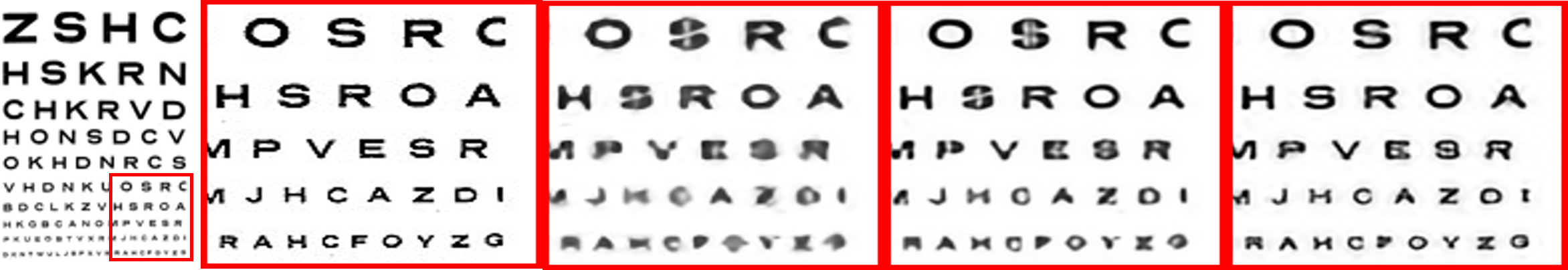
	Ground Truth	VDSR [8]	EDSR+ [12]	ZSSR (ours)
	(PSNR, SSIM)	(20.11, 0.9136)	(25.29 / 0.9627)	(25.68 / 0.9546)

Figure 5: In images with strong internal repetitive structures, ZSSR tends to surpass VDSR, and sometimes also EDSR+, even though the LR image was generated using the ‘ideal’ supervised setting (i.e., bicubic downscaling).

		Supervised			Unsupervised
Dataset	Scale	SRCNN [3]	VDSR [8]	EDSR+ [12]	SelfExSR [6]	ZSSR (ours)
Set5	$\times 2$	36.66 / 0.9542	37.53 / 0.9587	38.20 / 0.9606	36.49 / 0.9537	37.37 / 0.9570
	$\times 3$	32.75 / 0.9090	33.66 / 0.9213	34.76 / 0.9290	32.58 / 0.9093	33.42 / 0.9188
	$\times 4$	30.48 / 0.8628	31.35 / 0.8838	32.62 / 0.8984	30.31 / 0.8619	31.13 / 0.8796
Set14	$\times 2$	32.42 / 0.9063	33.03 / 0.9124	34.02 / 0.9204	32.22 / 0.9034	33.00 / 0.9108
	$\times 3$	29.28 / 0.8209	29.77 / 0.8314	30.66 / 0.8481	29.16 / 0.8196	29.80 / 0.8304
	$\times 4$	27.49 / 0.7503	28.01 / 0.7674	28.94 / 0.7901	27.40 / 0.7518	28.01 / 0.7651
BSD100	$\times 2$	31.36 / 0.8879	31.90 / 0.8960	32.37 / 0.9018	31.18 / 0.8855	31.65 / 0.8920
	$\times 3$	28.41 / 0.7863	28.82 / 0.7976	29.32 / 0.8104	28.29 / 0.7840	28.67 / 0.7945
	$\times 4$	26.90 / 0.7101	27.29 / 0.7251	27.79 / 0.7437	26.84 / 0.7106	27.12 / 0.7211

Table 1: Comparison of SR results for the ’ideal’ case (bicubic downscaling).

VDSR [8]	EDSR+ [12]	Blind-SR [14]	ZSSR [estimated kernel] (ours)	ZSSR [true kernel] (ours)
27.7212 / 0.7635	27.7826 / 0.7660	28.420 / 0.7834	28.8118 / 0.8306	29.6814 / 0.8414

Table 2: SR in the presence of unknown downscaling kernels. LR images were generated from the BSD100 dataset using random downscaling kernels (of reasonable size). SR$\times 2$ was then applied to those images. Please see text for more details.

Bicubic interpolation	EDSR+ [12]	ZSSR (ours)
27.9216 / 0.7504	27.5600 / 0.7135	28.6148 / 0.7809

Table 3: SR in the presence of unknown image degradation. Each LR image from the BSD100 dataset was randomly degraded using one of 3 types of degradations: (i) Gaussian noise, (ii) Speckle noise, (iii) JPEG compression. SR$\times 2$ was then applied to those images, without knowing the type of degradation. ZSSR shows robustness to unknown degradations, whereas SotA SR methods are not. In fact, under such conditions, bicubic interpolation outperforms current SotA SR methods.

4 Experiments & Results

Our method (ZSSR - ‘Zero-Shot SR’) is primarily aimed at real LR images obtained with realistic (unknown and varying) acquisition setting. These usually have no HR ground truth, hence are evaluated visually (as in Fig. 1). In order to quantitatively evaluate ZSSR’s performance, we ran several controlled experiments, on a variety of settings. Interestingly, ZSSR produces competitive results (although not SotA) on the ‘ideal’ benchmark datasets for which the SotA supervised methods train and specialize (even though our CNN is small, and has not been pretrained). However, on ‘non-ideal’ datasets, ZSSR surpasses SotA SR by a large margin. All reported numerical results were produced using the evaluation script of [8, 9].

4.1 The ‘Ideal’ Case

While this is not the aim of ZSSR, we tested it also on the standard SR benchmarks of ‘ideal’ LR images. In these benchmarks, the LR images are ideally downscaled from their HR versions using MATLAB’s $imresize$ command (a bicubic kernel downsampling with antialiasing). Table 1 shows that our image-specific ZSSR achieves competitive results against externally-supervised methods that were exhaustively trained for these conditions. In fact, ZSSR is significantly better than the older SRCNN [3], and in some cases achieves comparable or better results than VDSR [8] (which was the SotA until a year ago). Within the unsupervised-SR regime, ZSSR outperforms the leading method SelfExSR [6] by a large margin.

Moreover, in images with very strong internal repetitive structures, ZSSR tends to surpass VDSR, and sometimes also EDSR+, even though these LR images were generated using the ‘ideal’ supervised setting. One such example is shown in Fig. 5. Although this image is not a typical natural image, further analysis shows that the preference for internal learning (via ZSSR) exhibited in Fig. 5 exists not only in ‘fractal-like’ images, but is also found in general natural images. Several such examples are shown in Fig. 6. As can be seen, some of the pixels in the image (those marked in green) benefit more from exploiting internally learned data recurrence (ZSSR) over deeply learned external information, whereas other pixels (those marked in red) benefit more from externally learned data (EDSR+). As expected, the internal approach (ZSSR) is mostly advantageous in image area with high recurrence of information, especially in areas where these patterns are extremely small (of extremely low resolution), like the small windows in the top of the building. Such tiny patters find larger (high-res) examples of themselves elsewhere inside the same image (at a different location/scale). This indicates that there may be potential for further SR improvement (even in the ‘ideal’ bicubic case), by combining the power of Internal-Learning with External-Learning in a single computational framework. This remains part of our future work.

4.2 The ‘Non-ideal’ Case

Real LR images do not tend to be ideally generated. We have experimented with non-ideal cases that result from either: (i) non-ideal downscaling kernels (that deviate from the bicubic kernel), and (ii) low-quality LR images (e.g., due to noise, compression artifacts, etc.) In such non-ideal cases, the image-specific ZSSR provides significantly better results than SotA SR methods (by $1-2dB$). These quantities experiments are described next. Fig. 2 shows a few such visual results. Additional visual results and full images can be found in our project website.

(A) Non-ideal downscaling kernels:   The purpose of this experiment is to test more realistic blur kernels with the ability to numerically evaluate the results. For this purpose we created a new dataset from BSD100 [13] by downscaling the HR images using random (but reasonably sized) Gaussian kernels. For each image, the covariance matrix $\bf{\Sigma}$ of its downscaling kernel was chosen to have a random angle $\theta$ and random lengths $\lambda_{1},\lambda_{2}$ in each axis:

$$\lambda_{1},\lambda_{2} \backsim U[0,s^{2}]$$

$$\theta \backsim U[0,\pi]$$

$$\bf{\Lambda} =diag(\lambda_{1},\lambda_{2})$$

$$\bf{U} =\begin{bmatrix}\cos(\theta)&-\sin(\theta)\\ \sin(\theta)&\cos(\theta)\end{bmatrix}$$

$$\bf{\Sigma} =\bf{U\Lambda U^{t}}$$ (1)

where $s$ is the HR-LR downscaling factor. Thus, each LR image was subsampled by a different random kernel. Table 2 compares our performance against the leading externally-supervised SR methods [12, 8]. We also compared our performance to the unsupervised Blind-SR method of [14]. We considered two cases for applying ZSSR: (i) The more realistic scenario of unknown downscaling kernel. For this mode we used [14] to evaluate the kernel directly from the test image and fed it to ZSSR. The unknown SR kernel is estimated in [14] by seeking a non-parametric downscaling kernel which maximizes the similarity of patches across scales in the LR test image. (ii) We applied ZSSR with the true downscaling kernel used to create the LR image. Such a scenario is potentially useful for images obtained by sensors with known specs.

Note that none of the externally-supervised methods are able to benefit from knowing the blur kernel of the test image (whether estimated or real), since they were trained and optimized exhaustively for a specific kernel. Table 2 shows that ZSSR outperforms SotA methods by a very large margin: $+1db$ for unknown (estimated) kernels, and $+2db$ when provided the true kernels. Visually, the SR images generated by SotA methods are very blurry (see Fig. 2, and project website) . Interestingly, the unsupervised Blind-SR method of [14], which does not use any deep learning, also outperforms SotA SR methods. This further supports the analysis and observations of [17], that (i) an accurate donwscaling model is more important than sophisticated image priors, and (ii) using the wrong donwscaling kernel leads to oversmoothed SR results.

A special case of a non-ideal kernel is the $\delta$ kernel, which results in aliasing. This case too, is not handled well by SotA methods (see example in Fig. 2).

(B) Poor-quality LR images:   In this experiment, we tested images with different types of quality degradation. To test the robustness of ZSSR in coping with unknown damage, we chose for each image from BSD100 [13] a random type of degradation out of 3 degradations: (i) Gaussian noise [$\sigma=0.05$], (ii) Speckle noise [$\sigma=0.05$], (iii) JPEG compression [quality = 45 (By MATLAB standard)]. Table 3 shows that ZSSR is robust to unknown degradation types, while these typically damage SR supervised methods to the point where bicubic interpolation outperforms current SotA SR methods!

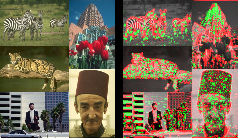
Figure 6: Internal vs. External preference. Green: pixels that favor Internal-SR (i.e., pixels where ZSSR obtains lower error with respect to the ground-truth HR image); Red: pixels that favour External-SR (EDSR+). Notice that edges (which are frequent in natural images) prefer External-SR, whereas unique image structures (e.g., the tiny windows at the top of the high building) prefer Internal-SR. Such tiny patters find larger (high-res) examples of themselves elsewhere inside the same image (at a different location/scale).

5 Conclusion

We introduce the concept of “Zero-Shot” SR, which exploits the power of Deep Learning, without relying on any external examples or prior training. This is obtained via a small image-specific CNN, which is trained at test time on internal examples extracted solely from the LR test image. This yields SR of real-world images, whose acquisition process is non-ideal, unknown, and changes from image to image (i.e., image-specific settings). In such real-world ‘non-ideal’ settings, our method substantially outperforms SotA SR methods, both qualitatively and quantitatively. To our best knowledge, this is the first unsupervised CNN-based SR method.

References

- [1] Y. Bahat, N. Efrat, and M. Irani. Non-uniform blind deblurring by reblurring. In ICCV, 2017.
- [2] Y. Bahat and M. Irani. Blind dehazing using internal patch recurrence. In ICCP, 2016.
- [3] K. H. X. T. Chao Dong, Chen Change Loy. Learning a deep convolutional network for image super-resolution. In European Conference on Computer Vision (ECCV), 2014.
- [4] S. B. D. Glasner and M. Irani. Super-resolution from a single image. In International Conference on Computer Vision (ICCV), 2009.
- [5] G. Freedman and R. Fattal. Image and video upscaling from local self-examples. ACM Transactions on Graphics, 30(2):12, 2011.
- [6] J.-B. Huang, A. Singh, and N. Ahuja. Single image super-resolution from transformed self-exemplars. In Proceedings of the IEEE Conference on Computer Vision and Pattern Recognition, pages 5197–5206, 2015.
- [7] M. Irani and S. Peleg. Improving resolution by image registration. CVGIP: Graphical Model and Image Processing, 53(3):231–239, 1991.
- [8] J. Kim, J. Kwon Lee, and K. Mu Lee. Accurate image super-resolution using very deep convolutional networks. In The IEEE Conference on Computer Vision and Pattern Recognition (CVPR) Workshops, pages 1646–1654, 06 2016.
- [9] J. Kim, J. K. Lee, and K. M. Lee. Deeply-recursive convolutional network for image super-resolution. In The IEEE Conference on Computer Vision and Pattern Recognition (CVPR Oral), June 2016.
- [10] D. P. Kingma and J. Ba. Adam: A method for stochastic optimization. CoRR, abs/1412.6980, 2014.
- [11] C. Ledig, L. Theis, F. Huszar, J. Caballero, A. Cunningham, A. Acosta, A. Aitken, A. Tejani, J. Totz, Z. Wang, and W. Shi. Photo-realistic single image super-resolution using a generative adversarial network. arXiv:1609.04802, 2016.
- [12] B. Lim, S. Son, H. Kim, S. Nah, and K. M. Lee. Enhanced deep residual networks for single image super-resolution. In The IEEE Conference on Computer Vision and Pattern Recognition (CVPR) Workshops, July 2017.
- [13] D. Martin, C. Fowlkes, D. Tal, and J. Malik. A database of human segmented natural images and its application to evaluating segmentation algorithms and measuring ecological statistics. In Proc. 8th Int’l Conf. Computer Vision, volume 2, pages 416–423, July 2001.
- [14] T. Michaeli and M. Irani. Nonparametric blind super-resolution. In International Conference on Computer Vision (ICCV), 2013.
- [15] T. Michaeli and M. Irani. Blind deblurring using internal patch recurrence. In European Conference on Computer Vision (ECCV). 2014.
- [16] I. Mosseri, M. Zontak, and M. Irani. Combining the power of internal and external denoising. In ICCP, 2013.
- [17] A. A. B. N. A. l. Netalee Efrat, Daniel Glasner. Accurate blur models vs. image priors in single image super-resolution. In ICCV, 2013.
- [18] A. Santoro, S. Bartunov, M. Botvinick, D. Wierstra, and T. P. Lillicrap. Meta-learning with memory-augmented neural networks. In International Conference on Machine Learning (ICML).
- [19] R. Timofte, E. Agustsson, M.-H. Van Gool, Luc Yang, L. Zhang, et al. Ntire 2017 challenge on single image super-resolution: Methods and results. In The IEEE Conference on Computer Vision and Pattern Recognition (CVPR) Workshops, July 2017.
- [20] R. Timofte, R. Rothe, and L. Van Gool. Seven ways to improve example-based single image super resolution. In The IEEE Conference on Computer Vision and Pattern Recognition (CVPR), June 2016.
- [21] R. Timofte, V. D. Smet, and L. V. Gool. A+: Adjusted anchored neighborhood regression for fast super-resolution. In ACCV, 2014.
- [22] Y. Xian, B. Schiele, and Z. Akata. Zero-shot learning – the Good, the Bad and the Ugly. In CVPR, 2017.
- [23] M. Zontak and M. Irani. Internal statistics of a single natural image. In IEEE Conference on Computer Vision and Pattern Recognition (CVPR), June 2011.
- [24] M. Zontak, I. Mosseri, and M. Irani. Separating signal from noise using patch recurrence across scales. In CVPR, 2013.