The fundamental Laplacian eigenvalue of the
regular polygon with Dirichlet boundary conditions

Abstract

The lowest eigenvalue of the Laplacian within the $S$-sided regular polygon with Dirichlet boundary conditions is the focus of this report. As suggested by others, this eigenvalue may be expressed as an asymptotic expansion in powers of $1/S$ where, interestingly, they have shown that the first few coefficients in that expansion, up to sixth order, may be expressed analytically in terms of Riemann zeta functions and roots of Bessel functions. This report builds on that work with three main contributions: (1) compelling numerical evidence independently supporting those published results, (2) a conjecture adding two more terms to the asymptotic expansion, and (3) an observation that higher-order coefficients both alternate in sign and grow rapidly in magnitude, which suggest the series doesn’t converge unless $S\!\geq\!10$. This report is based on a numerical computation of the eigenvalues precise to fifty digits for $S$ up to 150.

Keywords: Laplacian eigenvalue; regular polygon; asymptotic expansion

Introduction

Let $\Omega_{S}$ denote the interior of an $S$-sided regular polygon, and $\partial\Omega_{S}$ its boundary. The Laplacian eigenvalue problem with Dirichlet boundary conditions for that polygon is defined by

$$\left.\begin{array}[]{rl}\left[\Delta+\lambda\right]\Psi(\mathbf{r})=0&\text{ for $\mathbf{r}\in\Omega_{S}$}\\[4.30554pt] \Psi(\mathbf{r})=0&\text{ for $\mathbf{r}\in\partial\Omega_{S}$}\end{array}\right\}$$ (1)

where $\Delta$ is the two-dimensional Laplacian, $\lambda>0$ is an eigenvalue, and $\Psi(\mathbf{r})\not\equiv 0$ is a corresponding eigenfunction.

A given regular polygon has an infinite tower of eigenvalues, but this report shall focus only on the lowest (fundamental) eigenvalue, and, more specifically, an asymptotic expansion of the form

$$\lambda(S)\sim\widehat{\lambda}(S)\equiv j_{\text{\tiny 01}}^{2}\left[1+\sum_{\mu=1}^{\infty}\frac{C_{\mu}}{S^{\mu}}\right]=j_{\text{\tiny 01}}^{2}\left[1+\frac{C_{1}}{S}+\frac{C_{2}}{S^{2}}+\frac{C_{3}}{S^{3}}+\cdots\right]$$ (2)

where $j_{\text{\tiny 01}}^{2}\approx 5.7831$ is the lowest eigenvalue of the unit-radius circle. Since we don’t [yet] know how the expansion converges, make the distinction: $\lambda(S)$ denotes the exact fundamental eigenvalue for all $S=3,4,5,...$; whereas $\widehat{\lambda}(S)$ denotes its asymptotic expansion. When $\widehat{\lambda}(S)$ is truncated at $C_{N}/S^{N}$, i.e., to $N$th order, it shall be written $\widehat{\lambda}^{[N]}(S)$ so that

$$\lambda(S)\sim\widehat{\lambda}(S)=\widehat{\lambda}^{[N]}(S)+O(1/S^{N+1}).$$ (3)

Built into the series is the assumption that as the polygon approaches the unit-radius circle, i.e., in the limit $S\to\infty$, $\lambda(\infty)\!=\!\widehat{\lambda}(\infty)\!=\!j_{\text{\tiny 01}}^{2}$. This assumption seems natural, and is supported by numerics, but in passing, recall the curious polygon-circle paradox of thin-plate theory [8] where an analogous assumption breaks down.

When the area of $\Omega_{S}$ is held constant at $\pi$, i.e., the same area as the unit-radius circle, the proposed expansion to eighth order is

$$\widehat{\lambda}^{[8]}(S)=j_{\text{\tiny 01}}^{2}\left\{1+\frac{4\,\zeta(3)}{S^{3}}+\frac{\left[12-2j_{\text{\tiny 01}}^{2}\right]\,\zeta(5)}{S^{5}}+\frac{\left[8+4j_{\text{\tiny 01}}^{2}\right]\,\zeta^{2}(3)}{S^{6}}\right.\\[4.30554pt] \left.\mbox{}+\frac{\left[36-12j_{\text{\tiny 01}}^{2}-\frac{1}{2}\,j_{\text{\tiny 01}}^{4}\right]\,\zeta(7)}{S^{7}}+\frac{\left[48+8j_{\text{\tiny 01}}^{2}+2j_{\text{\tiny 01}}^{4}\right]\,\zeta(3)\zeta(5)}{S^{8}}\right\}$$ (4)

where $\zeta(n)=\sum_{\mu=1}^{\infty}\mu^{-n}$ is the well-known Riemann zeta function, and where the last two terms are contributions of this work.

The constant area of $\pi$ is chosen to more readily expose interesting facts about the eigenvalue and its asymptotic expansion. Doing so automatically factors out the well-known area rescaling dependence and simplifies the expressions. The Appendix details the relationship between this transcribed (equal area) regular polygon eigenvalue and the inscribed one, as well as some other relationships.

Over the last twenty years, a few others have considered this problem. A common theme is that those workers computed the eigen-solution while gradually deforming the circle into the regular polygon. In 1997, Molinari [7] suggested an expansion of $\sqrt{\lambda(S)}$ in powers of $1/S$ and used conformal mapping to estimate the leading coefficients of what he called a “partial resummation of terms in the $1/S$ expansion”, which he claimed improved convergence. In 2004, Grinfeld and Strang [3] proposed Eq. (2), and they used “the calculus of moving surfaces” (CMS) and numerics to estimate the first few coefficients. Although of limited numerical precision, these early efforts seemed promising and offered interesting insights.

More recently, in 2012, Grinfeld and Strang [4] revisited the problem and were able to express the coefficients up to $C_{4}$ as integer multiples of the Riemann zeta function. An interesting application of that work appears in 2010 when Oikonomou [10] studied the Casimir energy of a scalar field within a regular polygon. Several years later, in 2015, Boady [2], working with Grinfeld, and also using CMS, contributed two more terms, $C_{5}$ and $C_{6}$. Their results were obtained using a computer algebra system and do not depend on numerical computations per se. The terms up to sixth order – first line of Eq. (4) – shall be referred to as the Grinfeld-Strang-Boady [GSB] terms.

Of note is that only two solutions with finite $S$ are known in closed form, which for $\pi$-area $\Omega_{S}$ are

$$\lambda(3)=\frac{4\pi}{\sqrt{3}}\qquad\text{and}\qquad\lambda(4)=2\pi$$ (5)

All numerical evidence indicates that the $\pi$-area regular polygon eigenvalues are monotonic with $S$,

$$7.2552\approx\frac{4\pi}{\sqrt{3}}\geq\lambda(S)>\lambda(S+1)>j_{\text{\tiny 01}}^{2}\approx 5.7831$$ (6)

which is not unexpected [1, 9].

As terms are added to the asymptotic expansion per Eq. (4), interesting facts begin to emerge. For example, the Riemann zeta function arguments are (so far) chosen from $\{3,5,7,...\}$, and – within each term – sum to that term’s order. That pattern automatically requires $C_{1}=C_{2}=C_{4}=0$, which is a priori not obvious; and, for example, the eighth order term involves only $\zeta(3)\,\zeta(5)$ since $3+5$ is the only way to get $8$ from that set. Of course, each added term also brings us a little closer to identifying the elusive form of the function $\lambda(N)$ for which $\widehat{\lambda}(N)$ is merely its asymptotic expansion.

Of more practical interest is the ability to rapidly compute relatively high-precision eigenvalues. Indeed, using Eq. (4) and the computed, fifty-digit eigenvalues, the relative discrepancy is empirically determined to be

$$\frac{\widehat{\lambda}^{[8]}(S)-\lambda(S)}{\lambda(S)}\approx\frac{-18.38}{S^{7.86}}$$ (7)

apparently valid for all $S\!\geq\!5$. To illustrate, the ordinarily difficult-to-calculate $S\!=\!128$ eigenvalue is readily found to a precision of about fifteen digits,

$$\lambda(128) =5.78319922243209895\cdots\quad\text{(exact)}$$ (8)

$$\widehat{\lambda}^{[8]}(128) =5.78319922243209606\cdots$$ (9)

with a relative discrepancy of $-5.0\times 10^{-16}$, and where an ellipsis in a number indicates truncation, not rounding.

My approach is quite straightforward. It begins with a high-precision numerical computation [5] of the eigenvalues for $S$ from 5 to 150, precise to about fifty digits. These computed eigenvalues (skipping the lowest few) are then fit using linear regression to a truncated version of Eq. (2) with just under forty terms. My conjecture for the seventh and eighth order terms is derived using an LLL integer relation algorithm on the fit values of the coefficients. The list of computed eigenvalues, the LLL technique, and some other details are provided in the Appendix.

All computations were performed on my personal commodity hardware running free software with GNU/Linux (lubuntu 16.04.3 LTS) and its numerous ancillary utilities. For the eigenvalue computations, which took several months, I used a six-core (12-thread) i7-5820K @ 3.30 GHz with 64 GB RAM computer. Software of choice was the pari/gp [11] calculator (compiled with gmp and pthread). A few symbolic computations were performed using maxima [6].

Linear Regression

With the computed eigenvalues, linear regression shall be used to seek numerical values of the coefficients $C_{\mu}$ of Eq. (2). Because this process uses up to around forty coefficients and requires up to several dozen digits of precision, this unusual application of linear regression requires some computational caveats.

The numerically computed eigenvalues shall be denoted $\Lambda^{\text{[up]}}(S)$ and $\Lambda^{\text{[dn]}}(S)$ for the upper and lower bounds, respectively, or generically, $\Lambda(S)$ (which can refer to either bound or their mean). The relative difference between the computed bounds satisfies

$$(0.114)\times 10^{-50}<\frac{\Lambda^{\text{[up]}}(S)-\Lambda^{\text{[dn]}}(S)}{\Lambda(S)}<(0.998)\times 10^{-50}$$ (10)

which is just under $10^{-50}$, and with a mean of $(0.871)\times 10^{-50}$.

To develop the model equation, first let the independent variable be $X=1/S$. The dependent variable $Y$ shall incorporate (1) the computed eigenvalues, (2) the assumption that $\lambda(\infty)\!=\!j_{\text{\tiny 01}}^{2}$, and (3) analytic expressions for the coefficients. Initially, all coefficients are assumed unknown. Only after compelling numerical evidence supports an analytic expression for a coefficient shall that coefficient be considered known and exact, embellished with a tilde (so that $C_{\mu}$ becomes $\widetilde{C}_{\mu}$), and incorporated into $Y$.

Virtually nothing is published regarding the convergence of Eq. (2) except for the vague but obvious notion that convergence improves as $S$ increases. If we fit using low values of $S$ for which the asymptotic series doesn’t converge, the method will fail because it won’t capture the true nature of the function $\lambda(S)$. Therefore, the fit shall exclude the lowest few computed eigenvalues, and that fit used to conjecture convergence properties.

To make this work, as many coefficients as possible must be included in the fit, but not so many that the fit function begins to oscillate wildly as it tries to “connect the dots” with a polynomial in $X$. Also, because of the numerically ill-conditioned nature of the linear regression matrix computations, sufficient precision must be used. To that end, the precision of the linear regression computations is set to a more-than-adequate 200 digits. Both the number of terms to include in the expansion and the computation precision are established experimentally.

To estimate the precision of the coefficients, the upper and lower eigenvalue bounds are separately fit to the same model equation. This process yields two sets of numerical values for the coefficients, $\{C_{\mu}^{\text{[up]}}\}$ and $\{C_{\mu}^{\text{[dn]}}\}$, which incidentally do not form bounds. The relative difference and approximate number of digits in agreement between a pair of these numbers are, respectively,

$$\epsilon_{\mu}=\frac{C_{\mu}^{\text{[up]}}-C_{\mu}^{\text{[dn]}}}{\frac{1}{2}\left[C_{\mu}^{\text{[up]}}+C_{\mu}^{\text{[dn]}}\right]}\qquad\text{and}\qquad d_{\mu}=-\log_{10}\left|\epsilon_{\mu}\right|$$ (11)

In this report, a given coefficient shall be reported as the average value rounded one digit beyond a rounded $d_{\mu}$, along with the value of $d_{\mu}$. By example, if $C_{28}^{\mathrm{[up]}}=1.26128551\times 10^{16}$ and $C_{28}^{\mathrm{[dn]}}=1.26175766\times 10^{16}$, then this coefficient is reported as

$$C_{28}\ \{d_{28}\}=1.262\times 10^{16}\ \{3.4\}$$ (12)

where $\epsilon_{28}\!=\!-3.74\!\times\!10^{-4}$. Parameters are adjusted so that $d_{\mu}\!>\!1$ in every case.

Three important observations regarding the numerical values of the coefficients – looking down the series – include a drop in precision, an alternation in sign, and a growth in magnitude. These observations are quantified below.

In order to satisfy all the criteria, the following is chosen

Fit Parameters: (a) include up to $$C_{38} S=13,14,\cdots,150$$ and (b) use (13)

In hindsight, this will ensure that the minimum $S$-value is not too small, enough terms are included in the fit, and that every $d_{\mu}\!>\!1$.

There shall be four passes, of which the first three successfully establish the analytic set of coefficients depicted in Eq. (4). The final pass is used to estimate the remaining coefficients. With each pass, the number of unknown coefficients decreases, increasing their numerical precision slightly.

Pass 1

To begin, assume all of the first 38 coefficients are unknown and fit the computed eigenvalue data to the truncated series

$$Y_{a}\equiv S\cdot\left[\frac{\Lambda(S)}{j_{\text{\tiny 01}}^{2}}-1\right]=C_{1}+C_{2}X+C_{3}X^{2}+\cdots+C_{38}X^{37}$$ (14)

When this is done, the leading nine coefficients – listed in Table 1 – dramatically reveal that $C_{1}$, $C_{2}$, and $C_{4}$ range from thirty to forty orders of magnitude smaller than the nearby non-zero coefficients. Indeed, to the precision of the computation, they are effectively zero, which offers compelling numerical evidence in support of the GSB  result that

$$\framebox{$\widetilde{C}_{1}=\widetilde{C}_{2}=\widetilde{C}_{4}=0$}$$ (15)

Table 1: First pass results. The first nine and the last of 38 coefficients, assuming none are initially known per Eq. (14). Note the [near-]zero coefficients marked with arrows.

$\mu$	$C_{\mu}\ \{d_{\mu}\}$
1	$+0.0000000000000000000000000000000000000019\ \{1.4\}$  $\leftarrow$
2	$-0.0000000000000000000000000000000000039\ \{1.4\}$  $\leftarrow$
3	$+4.8082276126383771415989526460458038\ \{34.4\}$
4	$-0.0000000000000000000000000000023\ \{1.3\}$  $\leftarrow$
5	$+0.44964098545032430901630041787\ \{27.9\}$
6	$+44.98497175863112456004906931\ \{27.3\}$
7	$-50.539324388135164383037966\ \{24.9\}$
8	$+200.872237801870351587037\ \{23.1\}$
9	$-317.7704850739388022226\ \{21.1\}$
$\cdots$
38	$+2.53\times 10^{21}\ \{1.6\}$

Pass 2

Next, incorporate Eq. (15) into the dependent variable and refit the computed eigenvalue data to the model equation

$$Y_{b} \equiv S^{3}\cdot\left[\frac{\Lambda(S)}{j_{\text{\tiny 01}}^{2}}-1\right]=C_{3}+C_{5}X^{2}+C_{6}X^{3}+\cdots+C_{38}X^{35}$$ (16)

which now includes 35 terms in the expansion on the right hand side. The first three coefficients of the fit are then compared to the non-zero GSB  terms

$$\left.\begin{aligned} C_{3}\ \{d_{3}\}&=4.80822761263837714159895264604579996267\ \{38.0\}\\ 4\,\zeta(3)&=4.80822761263837714159895264604579996\raisebox{-3.22916pt}{\makebox[0.0pt]{\tiny$\blacktriangle$}}3059\cdots\end{aligned}\right\} \quad 36\ \text{digits}$$ (17)

$$\left.\begin{aligned} C_{5}\ \{d_{5}\}&=0.44964098545032430901630041683027\ \{30.8\}\\ (12-2j_{\text{\tiny 01}}^{2})\,\zeta(5)&=0.4496409854503243090163004168\raisebox{-3.22916pt}{\makebox[0.0pt]{\tiny$\blacktriangle$}}29603\cdots\end{aligned}\right\} \quad 28\ \text{digits}$$ (18)

$$\left.\begin{aligned} C_{6}\ \{d_{6}\}&\approx 44.98497175863112456004906966023\ \{29.8\}\\ (8+4j_{\text{\tiny 01}}^{2})\,\zeta(3)^{2}&=44.984971758631124560049069660\raisebox{-3.22916pt}{\makebox[0.0pt]{\tiny$\blacktriangle$}}994\cdots\end{aligned}\right\} \quad 29\ \text{digits}$$ (19)

where the number of digits in agreement is indicated. This result provides compelling numerical evidence supporting the remaining GSB  terms,

$$\framebox{$\widetilde{C}_{3}=4\,\zeta(3)$}\qquad\framebox{$\widetilde{C}_{5}=(12-2j_{\text{\tiny 01}}^{2})\,\zeta(5)$}\qquad\framebox{$\widetilde{C}_{6}=(8+4j_{\text{\tiny 01}}^{2})\,\zeta(3)^{2}$}$$ (20)

Pass 3

Next, incorporate the full GSB result, Eqs. (15) and (20), into the dependent variable and refit the computed eigenvalue data to the model equation

$$Y_{c} \equiv S^{7}\cdot\left[\frac{\Lambda(S)}{j_{\text{\tiny 01}}^{2}}-\left(1+\frac{\widetilde{C}_{3}}{S^{3}}+\frac{\widetilde{C}_{5}}{S^{5}}+\frac{\widetilde{C}_{6}}{S^{6}}\right)\right]=C_{7}+C_{8}X+\cdots+C_{38}X^{31}$$ (21)

which now includes 32 terms in the expansion on the right hand side. Comparing the resulting numerical coefficients $C_{7}$ and $C_{8}$ to the proposed expressions yields

$$\left.\begin{aligned} C_{7}\ \{d_{7}\}&=-50.53932438813516438303806289079\ \{30.4\}\\ \left(36-12j_{\text{\tiny 01}}^{2}-\mbox{$\frac{1}{2}$}j_{\text{\tiny 01}}^{4}\right)\,\zeta(7)&=-50.539324388135164383038062890\raisebox{-3.22916pt}{\makebox[0.0pt]{\tiny$\blacktriangle$}}904\cdots\end{aligned}\right\} \quad 29\ \text{digits}$$ (22)

$$\left.\begin{aligned} C_{8}\ \{d_{8}\}&=+200.87223780187035158705886400\ \{27.8\}\\ \left(48+8j_{\text{\tiny 01}}^{2}+2j_{\text{\tiny 01}}^{4}\right)\,\zeta(3)\,\zeta(5)&=+200.872237801870351587058864\raisebox{-3.22916pt}{\makebox[0.0pt]{\tiny$\blacktriangle$}}190\cdots\end{aligned}\right\} \quad 27\ \text{digits}$$ (23)

which provide compelling numerical evidence in support of my conjecture,

$$\framebox{$\widetilde{C}_{7}=\left(36-12j_{\text{\tiny 01}}^{2}-\frac{1}{2}j_{\text{\tiny 01}}^{4}\right)\,\zeta(7)$}\qquad\framebox{$\widetilde{C}_{8}=\left(48+8j_{\text{\tiny 01}}^{2}+2j_{\text{\tiny 01}}^{4}\right)\,\zeta(3)\zeta(5)$}$$ (24)

To discover the above relationships, the numerical coefficients, $C_{7}$ and $C_{8}$, are input into an LLL integer relation algorithm using

$$0 =a_{7}C_{7}+(b_{7}+c_{7}j_{\text{\tiny 01}}^{2}+d_{7}j_{\text{\tiny 01}}^{4})\,\zeta(7)$$ (25)

$$0 =a_{8}C_{8}+(b_{8}+c_{8}j_{\text{\tiny 01}}^{2}+d_{8}j_{\text{\tiny 01}}^{4})\,\zeta(3)\,\zeta(5)$$

where the respective four integers $\{a,b,c,d\}$ are sought. The form of the integer relation is guided by the GSB result. Details, including a computer program, are given in the Appendix.

Pass 4

Finally, incorporate Eqs. (15), (20), and (24) into the dependent variable and refit the computed eigenvalue data to the model equation

$$Y_{d}\equiv S^{9}\cdot\left[\frac{\Lambda(S)}{j_{\text{\tiny 01}}^{2}}-\left(1+\frac{\widetilde{C}_{3}}{S^{3}}+\frac{\widetilde{C}_{5}}{S^{5}}+\frac{\widetilde{C}_{6}}{S^{6}}+\frac{\widetilde{C}_{7}}{S^{7}}+\frac{\widetilde{C}_{8}}{S^{8}}\right)\right]\\ =C_{9}+C_{10}X+C_{11}X^{2}+\cdots+C_{38}X^{29}\qquad$$ (26)

which now includes 30 terms in the expansion on the right hand side. The complete results of this fit are shown in Table 2.

Table 2: Fourth pass results listing all thirty coefficients of the model Eq. (26). Note the sign alternation, growth in magnitude of $C_{\mu}$, and decrease in precision, $d_{\mu}$.

$\mu$	$C_{\mu}\ \{d_{\mu}\}$	$\mu$	$C_{\mu}\ \{d_{\mu}\}$
9	$-317.77048507393880222654502267\ \{27.5\}$	24	$+6.590391\times 10^{12}\ \{5.7\}$
10	$+1816.7620988762759616659826\ \{25.1\}$	25	$-4.19643\times 10^{13}\ \{5.0\}$
11	$-6016.33571769034682922143\ \{22.8\}$	26	$+2.7470\times 10^{14}\ \{4.4\}$
12	$+25200.97379293246467587\ \{20.9\}$	27	$-1.8436\times 10^{15}\ \{3.9\}$
13	$-93352.057545638041207\ \{19.0\}$	28	$+1.262\times 10^{16}\ \{3.4\}$
14	$+395412.696177504392\ \{17.2\}$	29	$-8.702\times 10^{16}\ \{3.0\}$
15	$-1718008.2767654300\ \{15.6\}$	30	$+5.934\times 10^{17}\ \{2.7\}$
16	$+7970543.96349877\ \{14.2\}$	31	$-3.89\times 10^{18}\ \{2.5\}$
17	$-38310267.955146\ \{12.8\}$	32	$+2.36\times 10^{19}\ \{2.3\}$
18	$+192454613.5202\ \{11.5\}$	33	$-1.27\times 10^{20}\ \{2.1\}$
19	$-1004632656.0\ \{10.3\}$	34	$+5.80\times 10^{20}\ \{2.0\}$
20	$+5.447327793\times 10^{9}\ \{9.2\}$	35	$-2.12\times 10^{21}\ \{1.9\}$
21	$-3.05943716\times 10^{10}\ \{8.2\}$	36	$+5.77\times 10^{21}\ \{1.8\}$
22	$+1.7770589\times 10^{11}\ \{7.3\}$	37	$-1.03\times 10^{22}\ \{1.8\}$
23	$-1.065749\times 10^{12}\ \{6.5\}$	38	$+8.96\times 10^{21}\ \{1.7\}$

Convergence

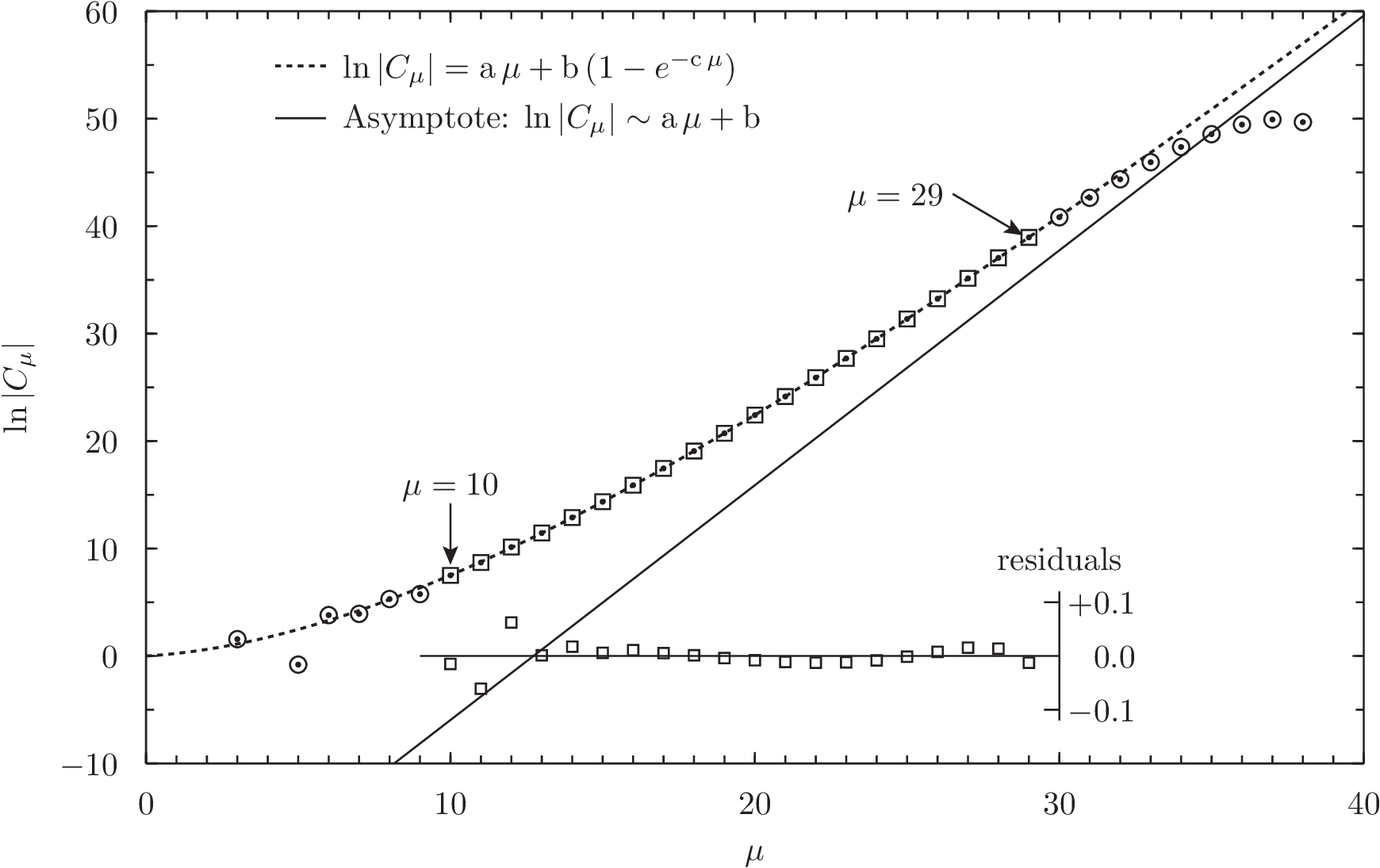
Figure 1: Coefficient growth. The coefficient data (Pass 2) are fit to a simple model using from $\mu=10$ to $29$, inclusive. (Circled data excluded from fit.) The inset displays the residuals of the points used in the fit on $50\times$ scale.

Numerically, the coefficients of Eq. (2) exhibit two important properties which can be seen clearly in Table 2. As one looks down that series, beyond the first few terms, the coefficients appear to both alternate in sign and grow in magnitude very rapidly, apparently consistent with

$$\begin{cases}\displaystyle C_{\mu}=(-1)^{\mu}|C_{\mu}|&\qquad\text{for $\mu>7$}\\ \ln\left|C_{\mu}\right|\sim\mathrm{a}\,\mu+\mathrm{b}&\qquad\text{as $\mu\to\infty$}\end{cases}$$ (27)

To analyze the coefficient growth, the natural logarithm of the absolute value of the non-zero coefficients is plotted against the series index in Fig. 1 (circled and squared dots). The down-turn in the last ten or so coefficients is an artifact of the truncation (here, at $\mu\!=\!38$). Also visible (at this scale) is that a smooth pattern isn’t established until $\mu\!\approx\!10$.

If “$\ln\left|C_{\mu}\right|$” does indeed approach a straight-line asymptote, the slope “$\mathrm{a}$” of that asymptote determines convergence. To see this, for sufficiently large but finite $N$, the remainder

$$R_{N}(S)\equiv\frac{\widehat{\lambda}(S)-\widehat{\lambda}^{[N\!-\!1]}(S)}{j_{\text{\tiny 01}}^{2}}=\sum_{\mu=N}^{\infty}\frac{C_{\mu}}{S^{\mu}}\approx e^{\mathrm{b}}\sum_{i=N}^{\infty}\displaystyle(-1)^{\mu}\left[\frac{e^{\mathrm{a}}}{S}\right]^{\mu}$$ (28)

certainly diverges if $S$ is too small. Indeed, the alternating geometric series in the last term is absolutely convergent if $S>e^{\mathrm{a}}$, and diverges otherwise. (Both $\mathrm{a}$ and $S$ are positive.) Since $\widehat{\lambda}^{[N]}(S)$ is finite, conclude that $\widehat{\lambda}(S)$ is absolutely convergent if and only if

$$S>S_{\text{cr}}\equiv e^{\mathrm{a}}\qquad\text{(critical $S$-value)}$$ (29)

The challenge is to determine the slope of the asymptote, presuming there is one. Without a known functional form for the coefficients, there must be some mathematical caution with this numerical exploration. The most straightforward technique is to fit the numerical values of the coefficients to a model with the simple criteria that it have as few parameters as possible and a built-in asymptote.

The model chosen here is the three-parameter exponential approach to the asymptote,

$$\ln\left|C_{\mu}\right|=\mathrm{a}\,\mu+\mathrm{b}\,\left(1-e^{-c\mu}\right)$$ (30)

Some numerical values are excluded from the fit to avoid both the artificial down-turn at the high end and the non-smooth behavior in the low end. For the current set of data, using $10\!\leq\!\mu\!\leq\!29$ yields

$$\left\{\begin{aligned} \mathrm{a}&=\phantom{+}2.185\pm 0.013\\ \mathrm{b}&=-27.81\pm 0.57\\ \mathrm{c}&=\phantom{+}0.07244\pm 0.0013\end{aligned}\right.$$ (31)

where the expected values and standard deviations are reported. This choice of model fits the data quite well and even extrapolates through the lower end as shown in Fig 1. The inset displays the residuals for the coefficients used in the fit. With these numbers,

$$S_{\text{cr}}=e^{\mathrm{a}}=8.89\pm 0.12=\underbrace{8.53\text{ to }9.25}_{6\sigma\ \text{interval}}$$ (32)

Other simple models yield values anywhere between 7 and 9, but none as large as 10. Erring on the side of caution, conclude that the asymptotic series converges if $S$ is at least $10$. In hindsight, since $S_{\text{cr}}\!<\!13$, this result is consistent with the fit parameters, Eq. (13), used to determine the coefficients.

Future

There is much room for future work. For example, it is tempting to search for yet higher-order coefficients and to study other eigenvalues of the regular polygon. Another direction is to establish more rigorous convergence criteria. Yet another higher goal is to establish an analytic form of $\lambda(S)$, not merely its asymptotic expansion.

Of note is that I am unable to extend the results to the ninth-order term (or higher). The natural extension of Eq. 25 might look like

$$0=a_{9}C_{9}+\left[b_{9}+c_{9}j_{\text{\tiny 01}}^{2}+d_{9}j_{\text{\tiny 01}}^{4}+e_{9}j_{\text{\tiny 01}}^{6}\right]\,\zeta(3)^{3}+\left[f_{9}+g_{9}j_{\text{\tiny 01}}^{2}+h_{9}j_{\text{\tiny 01}}^{4}+i_{9}j_{\text{\tiny 01}}^{6}\right]\,\zeta(9)$$ (33)

where the nine [small] integers $\{a_{9},b_{9},...,i_{9}\}$ must be determined – provided the Boady conjecture is somewhat valid. However, $C_{9}$ is computed here to only about 27 digits (Table 2), and the LLL routine does not suggest a unique solution as it does with the lower-order terms. The failure may be due to either a breakdown in the simple pattern or an insufficient precision for the LLL algorithm, or both.

Conclusion

This investigation of the asymptotic expansion of the fundamental Dirichlet eigenvalue of the Laplacian within the $S$-sided regular polygon leads to three original results:

1. independent and compelling numerical evidence in support of the GSB result,

2. a conjecture for the next two terms (seventh and eighth order), and

3. numerical evidence that the asymptotic series may converge only if $S\!\geq\!10$.

These results are obtained using fifty-digit computed eigenvalues for $S$ up to 150. Regression analysis of that data provides the evidence in support of the GSB result. The GSB result, together with an integer relation analysis of the numerical coefficients, leads to the conjecture for the next two terms with compelling numerical evidence supporting it. Looking further down the asymptotic series, a simple pattern (sign alternation and coefficient growth) emerged that suggests it may converge only if $S\!\geq\!10$.

Appendix

Relation to the GSB result The $S$-sided regular polygon used by others [7, 3, 10, 4, 2] is typically inscribed in a unit-radius circle. Grinfeld and Strang use the term transcribe to refer to an area-preserving circle-to-polygon deformation. Although I don’t deform a circle, the sequence ($S=3,4,5,...$) of $\pi$-area regular polygons shall herein be referred to as transcribed regular polygons to distinguish them from inscribed polygons, both in relation to that unit-radius circle.

To distinguish the two problems, a prime is placed on the inscribed problem variables. Thus

$$A(S)=\pi\qquad\text{ and }\qquad A^{\prime}(S)=S\cos\left(\frac{\pi}{S}\right)\sin\left(\frac{\pi}{S}\right)$$ (34)

are, respectively, the transcribed and inscribed area of the $S$-sided regular polygon. Note that $A^{\prime}(\infty)=\pi$, as required.

The area-rescaling relation for the eigenvalues is then either

$$\lambda(S)\,\pi=\lambda^{\prime}(S)A^{\prime}(S)\qquad\text{ or }\qquad\widehat{\lambda}(S)\,\pi=\widehat{\lambda}^{\prime}(S)\,A^{\prime}(S)$$ (35)

assuming $\widehat{\lambda}(S)$ and $\widehat{\lambda}^{\prime}(S)$ converge. By asymptotically expanding this, it is straightforward to show the relationship between the published GSB-result (inscribed) and my $\pi$-area (transcribed) result, as discussed around Eqs. 11.46 to 11.48 of the Boady thesis. The following, lightly-commented maxima [6] code will do that. Note that my maxima function g(S) is $\widehat{\lambda}^{[6]}(S)/j_{\text{\tiny 01}}^{2}$ and variable L is $j_{\text{\tiny 01}}^{2}$.

⬇

/* g(S) , for pi-area regular polygon, to sixth order */

g(S):=1 + 4*zeta(3)/S^3 + (12-2*L)*zeta(5)/S^5

+ (8+4*L)*zeta(3)*zeta(3)/S^6;

/* Area of inscribed regular polygon divided by pi */

A(S):=(S/%pi)*cos(%pi/S)*sin(%pi/S);

/* expand out to sixth order in powers of 1/S */

expr:taylor(g(S)/A(S),S,inf,6);

/* Kludge to express in terms of zeta functions. */

expr:expr,[%pi^2=6*Z(2),%pi^4=90*Z(4),%pi^6=945*Z(6),

zeta(3)=Z(3),zeta(5)=Z(5)];

/* The next line shows the GSB result, Boady thesis Eq. 11.46 */

collectterms(expand(ratsimp(expr)),S);

The transcribed and inscribed expressions are, respectively,

$$\widehat{\lambda}^{[6]}(S) =j_{\text{\tiny 01}}^{2}\,\left[1+\frac{4\,\zeta(3)}{S^{3}}+\frac{(12-2j_{\text{\tiny 01}}^{2})\,\zeta(5)}{S^{5}}+\frac{(8+4\,j_{\text{\tiny 01}}^{2})\,\zeta^{2}(3)}{S^{6}}\right]$$ (36)

$$\widehat{\lambda}^{[6]\prime}(S) =j_{\text{\tiny 01}}^{2}\,\left[1+\frac{4\,\zeta(2)}{S^{2}}+\frac{4\,\zeta(3)}{S^{3}}+\frac{28\,\zeta(4)}{S^{4}}\right.$$

$$+ \left.\frac{(12-2j_{\text{\tiny 01}}^{2})\,\zeta(5)+16\,\zeta(2)\,\zeta(3)}{S^{5}}+\frac{(8+4\,j_{\text{\tiny 01}}^{2})\,\zeta^{2}(3)+124\,\zeta(6)}{S^{6}}\right]$$ (37)

One thing to note is that terms with even zeta function arguments appear to be artifacts of the area dependence.

Relation to other eigenvalues

The focus of this report has been on the lowest eigenvalue. It is important to note that the asymptotic series may be readily modified for eigenvalues within the same symmetry class as the lowest one, i.e., those with $S$ even lines of symmetry intersecting at the polygon center. Indeed, some of the other efforts were not limited to the lowest eigenvalue. The extension is made by simply replacing $j_{\text{\tiny 01}}$ with the appropriate Bessel function root. See, for example, the Casimir energy analysis by Oikonomou [10].

LLL procedure

Below is a lightly-commented Pari gp-calculator program that applies an LLL integer-relation algorithm to the five coefficients using the gp routine qflll.

⬇

{

default(realprecision,100); \\ working precision, 100 digits

L0= (solve(x=sqrt(5.7),sqrt(5.8), besselj(0,x)))^2; \\ j_{01}^2

o = [3,5,6,7,8]; \\ vector of term orders

t = [1,2,2,3,3]; \\ number of terms in RHS

C = vector(#o); \\ numerical coefficients order

C[1] = 4.80822761263837714159895264604579996267; \\ 3

C[2] = 0.44964098545032430901630041683027; \\ 5

C[3] = 44.98497175863112456004906966023; \\ 6

C[4] = -50.53932438813516438303806289079; \\ 7

C[5] = 200.87223780187035158705886400; \\ 8

\\ Choosing zeta functions {3,5,6=3+3,7,8=3+5}

Z = [zeta(3), zeta(5), zeta(3)^2, zeta(7), zeta(3)*zeta(5)];

for (i=1, #o, \\ loop over the five terms

u = [C[i]]; \\ start off u-vector

u = concat(u, Z[i]*vector(t[i], j, L0^(j-1)));

N = #u;

p = 30; \\ rounding parameter

M = matid(N); \\ NxN identity matrix

M[N,]=round(u*10^p); \\ put numbers in last row

v = qflll(M)[,1]; \\ LLL routine, 1st col returned

v = sign(v[1])*v; \\ make v[1] positive

epsil = sum(j=1, #v, u[j]*v[j]); \\ ideally close to zero

relerr= abs(epsil/C[i]); \\ relative error

printf(”C_%d=%6.3f ”, o[i], C[i]);

printf(”relerr=%6.3g v=[%d”, relerr, v[1]);

for(j=1,t[i], printf(”,%d”, v[j+1])); printf(”]\n”);

);

}

For reference, the output is

⬇

C_3= 4.808 relerr=8.11 e-38 v=[1,-4]

C_5= 0.450 relerr=1.48 e-30 v=[1,-12,2]

C_6=44.985 relerr=1.70 e-29 v=[1,-8,-4]

C_7=-50.539 relerr=4.53 e-30 v=[2,-72,24,1]

C_8=200.872 relerr=9.46 e-28 v=[1,-48,-8,-2]

which can be used to construct the coefficients displayed in Eq. (4), including the non-zero GSB terms.

Computed eigenvalues

The computed eigenvalues upon which this work relies are listed in Table LABEL:tab:eigenvalues. This data represents a several-month computation, from July 22 to November 5, 2017. The computer time required for each eigenvalue increased with $S$ from a few seconds for $S\!=\!5$ to about 2.5 days at $S\!=\!150$.

Table 3: Computed fifty-digit Dirichlet eigenvalues of the Laplacian, per Eq. (1), for the $\pi$-area, $S$-sided regular polygon with $S$ up to $150$. By example, $\Lambda=5.12\,^{56}_{37}$ means $5.1237<\lambda<5.1256$. $\epsilon$ is the relative difference between upper and lower bounds. The first two eigenvalues are closed-form, and the last entry is the $S\!\to\!\infty$ circle eigenvalue.

$S$	$\Lambda$	$\epsilon\ (\times 10^{-51})$
$3$	$7.255197456936871402376313030568622929136264992370962\cdots=4\pi/\sqrt{3}$
$4$	$6.283185307179586476925286766559005768394338798750211\cdots=2\pi$
$5$	$6.02213793204263387829800871005424296700530534044855\,^{88}_{18}$	$1.14$
$6$	$5.9174178316136612156885745768389615450082860040929\,^{721}_{266}$	$7.67$
$7$	$5.8664493126559858577124749417588410842427349136980\,^{702}_{495}$	$3.52$
$8$	$5.8384914335924428505166403795638157848367571520259\,^{684}_{419}$	$4.52$
$9$	$5.821826802270265731735546443716945921671786764620\,^{6082}_{5822}$	$4.46$
$10$	$5.8112603592191160227888164688111646234421581749002\,^{717}_{159}$	$9.59$
$11$	$5.8042306367174007218783944528561768184219904268906\,^{603}_{187}$	$7.15$
$12$	$5.7993698043565000793150253110077586111011868022191\,^{607}_{300}$	$5.27$
$13$	$5.7959002668560147097907710633371318342893868231820\,^{486}_{260}$	$3.88$
$14$	$5.793357005271194553273227078683828691973872008926\,^{8251}_{7934}$	$5.45$
$15$	$5.791450010651579975693848498149681163522889425220\,^{2343}_{1931}$	$7.09$
$16$	$5.7899918999902085343497522138280801741824641952139\,^{910}_{405}$	$8.70$
$17$	$5.7888578719811046986171966351899455269041934747495\,^{463}_{110}$	$6.07$
$18$	$5.7879625918578468642125683801538930922402544098186\,^{443}_{032}$	$7.08$
$19$	$5.787246351381961243008036644834744747679263989712\,^{6307}_{5843}$	$8.01$
$20$	$5.7866665141403722135309129620257370578364779208083\,^{802}_{290}$	$8.84$
$21$	$5.7861920775968442730282037573295124400580514989647\,^{594}_{040}$	$9.56$
$22$	$5.7858001294283650275745860443434083658465152450013\,^{521}_{126}$	$6.81$
$23$	$5.7854734864549016320482640701967564443197042731253\,^{729}_{441}$	$4.96$
$24$	$5.785199089790024091834463612979690633039598488051\,^{8322}_{7878}$	$7.66$
$25$	$5.7849668941304235014186706838851226120341859263223\,^{965}_{502}$	$7.98$
$26$	$5.7847690863148429779922747176926528381622936339967\,^{445}_{104}$	$5.88$
$27$	$5.7845995272364846405932228271557722785394731147071\,^{640}_{151}$	$8.44$
$28$	$5.7844533477517199511967948423990305225015801633632\,^{812}_{448}$	$6.28$
$29$	$5.784326652365411207380293385946299260682128920466\,^{5349}_{4846}$	$8.68$
$30$	$5.784216299392264044119036734072080273019850029152\,^{1071}_{0693}$	$6.53$
$31$	$5.784119736080032703344528384598811278461255613439\,^{3095}_{2588}$	$8.75$
$32$	$5.784034873702444318330507486930290862975888102019\,^{3253}_{2867}$	$6.65$
$33$	$5.783959992040508812335032522628621979446533803257\,^{2140}_{1637}$	$8.69$
$34$	$5.7838936656948092520334765687133149515574394886548\,^{910}_{410}$	$8.62$
$35$	$5.7838347067709882028407000052233665412473857264158\,^{612}_{227}$	$6.64$
$36$	$5.783782119955880627699919965851270952506815797405\,^{8288}_{7800}$	$8.42$
$37$	$5.783735067049846291962440636524259616676854699958\,^{3345}_{2864}$	$8.30$
$38$	$5.7836928387732922677065179222622535502538886661416\,^{934}_{461}$	$8.16$
$39$	$5.7836548322108711433862079109147809210199222742790\,^{551}_{087}$	$8.02$
$40$	$5.783620532655973576951368558889088191821701701593\,^{5398}_{4942}$	$7.87$
$41$	$5.783589498912728857243541087541613440608196223660\,^{2233}_{1681}$	$9.53$
$42$	$5.783561351331960679963744950469531484077839530288\,^{6533}_{5995}$	$9.29$
$43$	$5.7835357620219719712774467620660707772186262259777\,^{895}_{372}$	$9.04$
$44$	$5.783512446799268033474803357987667934572313002680\,^{7317}_{6808}$	$8.79$
$45$	$5.783491158538856302913858878804287379136291682036\,^{6143}_{5647}$	$8.55$
$46$	$5.7834716816561681101051372252375789382247863870892\,^{595}_{113}$	$8.31$
$47$	$5.783453827508463297379645913916576075154358289917\,^{3155}_{2592}$	$9.72$
$48$	$5.7834374305468654192506360647558848068434756772524\,^{645}_{100}$	$9.41$
$49$	$5.783422345083940177286945516586288853576803572305\,^{1365}_{0838}$	$9.11$
$50$	$5.7834084425682129947801161963236469590292923516017\,^{854}_{343}$	$8.82$
$51$	$5.7833956092779034421663981399445418601302161224952\,^{893}_{399}$	$8.53$
$52$	$5.7833837443627027000195590153219733045460685739016\,^{742}_{177}$	$9.76$
$53$	$5.7833727581755982440480496612883417072850762249903\,^{706}_{160}$	$9.42$
$54$	$5.7833625708472927428973141440030573413552170062\,^{900473}_{899947}$	$9.09$
$55$	$5.783353111064236385644810842163192250719443038200\,^{6093}_{5585}$	$8.77$
$56$	$5.78334431501812935463844781588756191043588875765\,^{40427}_{39854}$	$9.89$
$57$	$5.7833361255002921030903693546648597586536448335457\,^{618}_{066}$	$9.53$
$58$	$5.7833284911188091539136722748217426193090792309470\,^{845}_{313}$	$9.18$
$59$	$5.7833213656200338537379396114645869789760826156081\,^{794}_{282}$	$8.84$
$60$	$5.783314707299059428210797800183990949668498895119\,^{6345}_{5774}$	$9.86$
$61$	$5.783308478486244250571058736219661811034316213866\,^{3113}_{2564}$	$9.48$
$62$	$5.7833026450989284101703805978440170235282052458579\,^{531}_{002}$	$9.13$
$63$	$5.783297176249175699422050587208076227946408600731\,^{7365}_{6856}$	$8.79$
$64$	$5.7832920438997850274611258286193147488559177241149\,^{925}_{364}$	$9.70$
$65$	$5.783287222561990216101379318958387384571634250267\,^{3215}_{2675}$	$9.32$
$66$	$5.7832826890292492111478490456613641227808808137750\,^{732}_{212}$	$8.97$
$67$	$5.783278422142346980297970170232395388356378905112\,^{1470}_{0900}$	$9.83$
$68$	$5.783274402581728387648667336549538768975499369192\,^{6319}_{5771}$	$9.45$
$69$	$5.7832706126835606254665067931060003616486874965111\,^{554}_{028}$	$9.08$
$70$	$5.783267036276517720104953505291690754885783103053\,^{3438}_{2865}$	$9.89$
$71$	$5.7832636585366972675053570571575828141496986506519\,^{916}_{366}$	$9.50$
$72$	$5.7832604658584342703907945644030276005726248720419\,^{576}_{046}$	$9.14$
$73$	$5.7832574457390789460408703608938752178996635604860\,^{577}_{004}$	$9.90$
$74$	$5.7832545866760630843215845592704878980855033362418\,^{808}_{257}$	$9.51$
$75$	$5.7832518780747999519072844129240886957218156591922\,^{670}_{141}$	$9.14$
$76$	$5.7832493101661516716346291929211527006058362175622\,^{945}_{374}$	$9.85$
$77$	$5.7832468739323602985306185231341800220529994071590\,^{639}_{150}$	$8.45$
$78$	$5.783244561040478512305563118717910086346504177634\,^{6472}_{5945}$	$9.09$
$79$	$5.7832423637824563386561208792114744191451563621838\,^{703}_{137}$	$9.76$
$80$	$5.7832402750211444434602632903336057637956537641100\,^{733}_{246}$	$8.41$
$81$	$5.783238288141564708788818913744019150004231228987\,^{6027}_{5504}$	$9.01$
$82$	$5.7832363970068770166311668301521069133506020689353\,^{844}_{285}$	$9.64$
$83$	$5.78323459591853914193516915928294052374939682204\,^{30082}_{29599}$	$8.34$
$84$	$5.78323287958021583661957400684452483337094433777\,^{80111}_{79539}$	$9.87$
$85$	$5.783231243065044797761869159688729531153474161960\,^{8425}_{7929}$	$8.57$
$86$	$5.7832296817859122999872941895330211636707297244341\,^{803}_{275}$	$9.12$
$87$	$5.7832281914684307238009975309857996746289319161078\,^{918}_{356}$	$9.69$
$88$	$5.783226768126344787904121271120141989640291161915\,^{8089}_{7600}$	$8.44$
$89$	$5.783225408039123644386441987435525040163562180818\,^{3249}_{2730}$	$8.96$
$90$	$5.783224107731522678222767981643965415039391863402\,^{5443}_{4893}$	$9.49$
$91$	$5.783222863954922345132559440101223356983832893756\,^{4446}_{3917}$	$9.12$
$92$	$5.783221673670272096140477542110521995453407740228\,^{7388}_{6879}$	$8.78$
$93$	$5.7832205340324857277389860275897345239229247945415\,^{675}_{138}$	$9.27$
$94$	$5.7832194423761506695184080213013434106581037042669\,^{600}_{033}$	$9.78$
$95$	$5.7832183962024280411626163932933568556831624568013\,^{978}_{433}$	$9.41$
$96$	$5.783217393167033007010852241398377430861882282949\,^{2327}_{1753}$	$9.90$
$97$	$5.783216431069196227758518741530320098257066954853\,^{8270}_{7765}$	$8.71$
$98$	$5.783215507841517228010683796245184675675966031085\,^{8128}_{7597}$	$9.16$
$99$	$5.783214621540629415561788196159738903682817178900\,^{4118}_{3560}$	$9.62$
$100$	$5.783213770338604434367144876070106403216402193565\,^{4364}_{3827}$	$9.26$
$101$	$5.7832129525150306224265566440583980748230299905146\,^{534}_{018}$	$8.91$
$102$	$5.783212166449706678032327479127825448347817055273\,^{1180}_{0639}$	$9.34$
$103$	$5.783211410615897300382237922986464486484414973146\,^{3446}_{2880}$	$9.78$
$104$	$5.783210683574102639949628780569819360526210833755\,^{8062}_{7560}$	$8.66$
$105$	$5.783209983966297937380176592129591988164382058292\,^{3293}_{2723}$	$9.84$
$106$	$5.783209310510603806034215145692410082844657773366\,^{6300}_{5794}$	$8.72$
$107$	$5.7832086619963512745011282308896272842754873361699\,^{771}_{243}$	$9.11$
$108$	$5.7832080372795089971773313237835737211106455961164\,^{988}_{437}$	$9.51$
$109$	$5.7832074352784430036203824301621058164531928714376\,^{652}_{077}$	$9.92$
$110$	$5.783206854969982026448346069044505432273217666833\,^{1081}_{0569}$	$8.82$
$111$	$5.783206295385763854495868384691346982424634552152\,^{1382}_{0850}$	$9.19$
$112$	$5.783205755608840330598899278697864669617886870683\,^{4198}_{3644}$	$9.57$
$113$	$5.7832052347705205764174624901385415125593493624890\,^{856}_{280}$	$9.95$
$114$	$5.7832047320474338019919255227789909098567095792232\,^{862}_{347}$	$8.88$
$115$	$5.7832042466587946646835703161902916564434900898372\,^{578}_{002}$	$9.95$
$116$	$5.783203777863855598037977272725438352252698382214\,^{6403}_{5888}$	$8.89$
$117$	$5.78320332495953185129119383617831568697480390758\,^{30315}_{29780}$	$9.23$
$118$	$5.7832028872781861783972732175519624981091930701562\,^{574}_{019}$	$9.58$
$119$	$5.7832024641855612037927177369523705379144297168954\,^{592}_{017}$	$9.93$
$120$	$5.7832020550788484815190743450796360573620493874627\,^{710}_{156}$	$9.57$
$121$	$5.783201659384884164529487670253652645264573710311\,^{4258}_{3724}$	$9.22$
$122$	$5.7832012765584620207102095560653892586849534945666\,^{979}_{426}$	$9.55$
$123$	$5.783200906080755279143481813903136517206041981035\,^{3386}_{2814}$	$9.87$
$124$	$5.783200547457839471403393668939526347739671446805\,^{1004}_{0452}$	$9.52$
$125$	$5.7832002002193090544707614611862501293189148764360\,^{754}_{184}$	$9.84$
$126$	$5.783199863916981169795599727550027796605983950656\,^{5444}_{4894}$	$9.48$
$127$	$5.783199538123680412174552013868591251347340966166\,^{6035}_{5505}$	$9.15$
$128$	$5.783199222432098956985238320133014718214303003483\,^{5340}_{4793}$	$9.44$
$129$	$5.783198916453726829015452454213861349980377100531\,^{3297}_{2733}$	$9.74$
$130$	$5.783198619817847494322697718282907407501883505901\,^{3379}_{2835}$	$9.40$
$131$	$5.783198332170594321576460839361900033150683319289\,^{3283}_{2758}$	$9.07$
$132$	$5.783198053174063794165401631077445539852104232715\,^{8325}_{7747}$	$9.98$
$133$	$5.7831977825054816616973973974236090228425636259915\,^{783}_{225}$	$9.63$
$134$	$5.783197519856418501824964777729256102794211740624\,^{6034}_{5460}$	$9.91$
$135$	$5.78319726493205142280133747938195184354472751162\,^{40300}_{39781}$	$8.97$
$136$	$5.783197017450468875813125929970793135181216310333\,^{2208}_{1673}$	$9.23$
$137$	$5.7831967771420157657553791022485248591356074629077\,^{779}_{228}$	$9.50$
$138$	$5.783196543748676251355969965179691633199779643683\,^{3230}_{2699}$	$9.17$
$139$	$5.78319631702349181190803820593767295255592560127\,^{10466}_{09919}$	$9.43$
$140$	$5.7831960967300123296839310805154072611401163978360\,^{776}_{215}$	$9.69$
$141$	$5.7831958826417780956100870897864370536602334172115\,^{593}_{016}$	$9.95$
$142$	$5.78319567454183079209634447072860419375002513070\,^{20001}_{19477}$	$9.03$
$143$	$5.7831954722222516420511547774247258923709033792146\,^{705}_{134}$	$9.86$
$144$	$5.783195275483725038000991945505785473982967396266\,^{5381}_{4829}$	$9.52$
$145$	$5.783195084135126080710376077178119900703268965184\,^{8025}_{7492}$	$9.20$
$146$	$5.783194897993130563536383404875214594259743023232\,^{7540}_{6993}$	$9.43$
$147$	$5.7831947168818460376488389106165087799453564413638\,^{878}_{318}$	$9.67$
$148$	$5.78319454063246268484401771071146302825917616988\,^{20197}_{19656}$	$9.34$
$149$	$5.7831943690829228095596336817453011340629123532482\,^{985}_{431}$	$9.57$
$150$	$5.7831942020776078403959106662108900488674959487428\,^{954}_{386}$	$9.80$

$\infty$

&   $5.783185962946784521175995758455807035071441806423685\cdots=j_{\text{\tiny 01}}^{2}$

References

- [1] P. Antunes and P. Freitas. New bounds for the principal Dirichlet eigenvalue of planar regions. Experimental Mathematics, 15:333–342, 2006.
- [2] Mark Boady. Applications of Symbolic Computation to the Calculus of Moving Surfaces. PhD thesis, Drexel University, Philadelphia, PA, 2015.
- [3] P. Grinfeld and G. Strang. The Laplacian eigenvalues of a polygon. Computers and Mathematics with Applications, 48:1121–1133, 2004.
- [4] P. Grinfeld and G. Strang. Laplace eigenvalues on regular polygons: A series in . J. Math. Anal. Appl., 385:135–149, 2012.
- [5] Robert Stephen Jones. Computing ultra-precise eigenvalues of the Laplacian within polygons. Advances in Computational Mathematics, May 2017.
- [6] Maxima. Maxima, a Computer Algebra System. Version 5.32. http://maxima.sourceforge.net/, 2017.
- [7] Luca Molinari. On the ground state of regular polygonal billiards. J. Phys. A: Math. Gen., 30(18):6517–6424, 1997.
- [8] N. W. Murray. The polygon-circle paradox and convergence in thin plate theory. Mathematical Proceedings of the Cambridge Philosophical Society, 73(1):279–282, 1973.
- [9] Carlo Nitsch. On the first Dirichlet Laplacian eigenvalue of regular polygons. Kodai Mathematical Journal, 37:595–607, 2014. http://arxiv.org/abs/1403.6709.
- [10] V. K. Oikonomou. Casimir energy for a regular polygon with Dirichlet boundaries. 2010. http://arxiv.org/abs/1012.5376.
- [11] The PARI Group, Univ. Bordeaux. PARI/GP version 2.9.3, 2017. Available online http://pari.math.u-bordeaux.fr/.