On $L_{p}$-error of bivariate polynomial
interpolation on the square

Abstract.

We obtain estimates of the $L_{p}$-error of the bivariate polynomial interpolation on the Lissajous-Chebyshev node points for wide classes of functions including non-smooth functions of bounded variation in the sense of Hardy-Krause. The results show that $L_{p}$-errors of polynomial interpolation on the Lissajous-Chebyshev nodes have almost the same behavior as the polynomial interpolation in the case of the tensor product Chebyshev grid.

1. Introduction

Let $B(D)$ be the set of all real-valued bounded measurable functions $f$ on some non-empty set $D\subset{\mathbb{R}}^{d}$. Denote ${\bm{k}}=(k_{1},\dots,k_{d})\in{{\mathbb{Z}}}_{+}^{d}$, ${\bm{n}}=(n_{1},\dots,n_{d})\in{{\mathbb{N}}}^{d}$, and ${\bm{x}}=(x_{1},\dots,x_{d})\in D$. Let $X_{\bm{n}}=\{{\bm{x}}_{\bm{k}}\}_{{\bm{k}}\in{\mathcal{I}}_{{\bm{n}}}}$ be a set of distinct points ${\bm{x}}_{\bm{k}}=(x_{1}^{({\bm{k}})},\dots,x_{d}^{({\bm{k}})})\in D$, where ${\mathcal{I}}_{{\bm{n}}}\subset{{\mathbb{Z}}}_{+}^{d}$ is the index set related to $X_{\bm{n}}$; let $\Pi_{\bm{n}}$ be some abstract space of polynomial functions on $D$ (e.g. algebraic or trigonometric polynomials of order at most ${\bm{n}}$ in some sense).

The polynomial interpolation problem associated to $X_{\bm{n}}$ and $\Pi_{\bm{n}}$ is to find for each $f\in B(D)$ a polynomial $P\in\Pi_{\bm{n}}$ such that

(1.1) $$P({\bm{x}}_{{\bm{k}}})=f({\bm{x}}_{{\bm{k}}})\quad\text{for all}\quad{\bm{k}}\in{\mathcal{I}}_{{\bm{n}}}.$$

If this problem is solvable, then one can construct the so-called Lagrange interpolation polynomial

$$L(f,X_{\bm{n}},{\bm{x}})=\sum_{{\bm{k}}\in{\mathcal{I}}_{{\bm{n}}}}f({\bm{x}}_{\bm{k}})\ell_{{\bm{k}}}(X_{\bm{n}},{\bm{x}}),$$

where $\ell_{{\bm{k}}}(X_{\bm{n}},{\bm{x}})\in\Pi_{\bm{n}}$ are fundamental Lagrange polynomials, i.e. $\ell_{{\bm{k}}}(X_{\bm{n}},{\bm{x}}_{\bm{l}})={\delta}_{{\bm{l}},{\bm{k}}}$ for all ${\bm{l}},{\bm{k}}\in{\mathcal{I}}_{\bm{n}}$ (${\delta}_{{\bm{l}},{\bm{k}}}$ is the Kronecker delta). In this case, we have

(1.2) $$L(f,X_{\bm{n}},{\bm{x}}_{\bm{k}})=f({\bm{x}}_{\bm{k}})\quad\text{for all}\quad{\bm{k}}\in{\mathcal{I}}_{\bm{n}}.$$

Everywhere below we will suppose that (1.1) is solvable and

(1.3) $$L(P,X_{\bm{n}},{\bm{x}})=P({\bm{x}})\quad\text{for all}\quad P\in\Pi_{\bm{n}}.$$

One of the main problems in multivariate polynomial interpolation is the choice of a suitable set of node points $X_{{\bm{n}}}$, which should provide ”​good” properties of the interpolation polynomials $L(f,X_{\bm{n}},{\bm{x}})$ depending on considered tasks. In the bivariate interpolation on $[-1,1]^{2}$, efficient node points were introduced by Morrow and Patterson [21], Xu [29] (see also [13]), Caliari, De Marchi, Vianello [5]. The set of points introduced in [5] are known as the so-called Padua points. It turned out that the Padua points are a promising set of nodes for bivariate polynomial interpolation. In particular, this point set allows unique interpolation in the appropriate space of polynomials; the Lebesgue constant of the interpolation problem on the Padua points grows only logarithmically with respect to the total degree of the interpolating polynomial; the Padua points can be characterized as a set of node points of a particular Lissajous curve [2]. The last property can be applied in a new medical imaging technology called Magnetic Particle Imaging. The main reason of this application is that the data acquisition path of the scanning device is commonly described by the Lissajous curves (see e.g. [16]). Under investigation of the bivariate polynomial interpolation of data values on these curves it was gained several extensions of the generating curve approach of the Padua points in [10] and [11] (see also the survey [12]).

Let us recall that in the bivariate setting the Lissajous curve ${\gamma}_{{\bm{n}}}:{\mathbb{R}}\to J^{2}$, $J=[-1,1]$, is given by

$${\gamma}_{{\bm{n}}}(t)=\left(\cos(n_{2}t),\cos(n_{1}t)\right),$$

where $n_{1}$ and $n_{2}$ are relatively prime. If we sample the curve ${\gamma}_{{\bm{n}}}$ along $n_{1}n_{2}+1$ equidistant points on $[0,\pi]$, then we get the set

$${\rm LC}_{{\bm{n}}}=\left\{{\gamma}_{{\bm{n}}}\left(\frac{\pi k}{n_{1}n_{2}}\right),\,k=0,\dots,n_{1}n_{2}\right\}$$

called the Lissajous-Chebyshev node points of the (degenerate) Lissajous curve (see [10]). Note that in the case $n_{2}=n_{1}+1$ the Lissajous-Chebyshev node points ${\rm LC}_{{\bm{n}}}$ coincide with the Padua points ${\rm Pad}_{n_{1}}$ (see [5], [2]).

The multivariate Lagrange interpolation on the Lissajous-Chebyshev node points was studied in detail in the recent papers [10], [6], and [7]. In particular, the following estimate of the error of approximation by the interpolation polynomials $L(f,{\rm LC}_{{\bm{n}}},\cdot)$ was obtained in [7]: if $\frac{\partial^{r}}{\partial^{r}x_{1}}f$, $\frac{\partial^{s}}{\partial^{s}x_{2}}f\in C(J^{2})$, then

(1.4) $$\|f-L(f,{\rm LC}_{{\bm{n}}},\cdot)\|_{L_{\infty}(J^{2})}=\mathcal{O}(\log n_{1}\log n_{2})\left(\frac{1}{{n_{1}}^{r}}+\frac{1}{{n_{2}}^{s}}\right).$$

Note that the polynomial $L(f,{\rm LC}_{{\bm{n}}},\cdot)$ has total degree at most $n_{1}+n_{2}-1$. Precisely, it has degree $n_{1}-1$ in $x_{1}$ and degree $n_{2}$ in $x_{2}$ (see also Theorem 3.1 and Theorem 3.2 below).

Concerning approximation in the weighted $L_{p,w}(J^{2})$ space with the Chebyshev weight $w(x_{1},x_{2})=1/{(\sqrt{1-x_{1}^{2}}\sqrt{1-x_{2}^{2}})^{\frac{1}{p}}}$, it is only known convergence (see [10]):

if $f\in C(J^{2})$ and $1\leq p<\infty$, then

(1.5) $$\|f-L(f,{\rm LC}_{{\bm{n}}},\cdot)\|_{L_{p,w}(J^{2})}\to 0\quad\text{\emph{as}}\quad\min\{n_{1},n_{2}\}\to\infty.$$

Results of qualitative type were considered only in the case of the Padua points (see [4]):

if $f\in C(J^{2})$, then

$$\|f-L(f,{\rm Pad}_{n},\cdot)\|_{L_{p,w}(J^{2})}\leq C_{p}E(f,\mathcal{P}_{n}^{2})_{\infty},$$

where $E(f,\mathcal{P}_{n}^{2})_{\infty}$ is the error of the best approximation of $f$ by polynomials from $\mathcal{P}_{n}^{2}$ (bivariate algebraic polynomials of degree $n$ in two variables) in the uniform metric.

Note that analogues of (1.4) and (1.5) for the Xu points, the Padua points, and the Lissajous-Chebyshev node points of the non-degenerate Lissajous curve were derived in [2], [3], [29], and [12].

In this paper, we obtain estimates of the error $\|f-L(f,{\rm LC}_{{\bm{n}}},\cdot)\|_{L_{p,w}(J^{2})}$ for wide classes of functions including non-smooth functions of bounded variation. In particular, we show that if a bivariate function $f$ has bounded variation in the sense of Hardy-Krause (see the definition in Section 4), then

(1.6) $$\|f-L(f,{\rm LC}_{{\bm{n}}},\cdot)\|_{L_{p,w}(J^{2})}=\mathcal{O}\left(\frac{1}{{n_{1}}^{1/p}}+\frac{1}{{n_{2}}^{1/p}}\right),$$

see Corollary 4.1.

A main idea of the proof of (1.6) is that using Marcinkiewicz-Zygmund-type inequalities and the fact that ${\rm LC}_{{\bm{n}}}$ is a subset of a certain set of points that forms the tensor product Chebyshev grid (see Figure 1), we can estimate the $L_{p}$-norm of the difference $f-L(f,{\rm LC}_{{\bm{n}}},\cdot)$ via the $L_{p}$-norm of the error of approximation of $f$ by some tensor product interpolation polynomials (see Lemma 5.10). Then we can apply some known results for classical interpolation polynomials, e.g. [22], [24], or [25].

The paper is organized as follows: In Section 2 we consider an abstract interpolation problem and obtain two types of estimates for the error of approximation of functions by interpolation polynomials. In Section 3 we give preliminary results and some notations related to the polynomial interpolation on the Lissajous-Chebyshev nodes. In Section 4 we formulate the main results. In Section 5 we prove auxiliary and main results of the paper.

2. General estimates of the error of approximation by interpolation polynomials

Let $B_{p}(D)$, $1\leq p<\infty$, be a subspace of $B(D)$ equipped with the norm $\|f\|_{p}=\|f\|_{B_{p}(D)}$. Everywhere below we suppose that the set of polynomials $\Pi_{\bm{n}}$ is a subset of $B_{p}(D)$ for any $1\leq p<\infty$.

Let us consider generalized Marcinkiewicz-Zygmund (MZ) inequalities associated with a norm $\|\cdot\|_{p}$, node points $X_{\bm{n}}$, weights ${\Lambda}_{\bm{n}}=\{{\lambda}_{\bm{k}}\}_{{\bm{k}}\in{\mathcal{I}}_{\bm{n}}}\subset{\mathbb{R}}_{+}^{d}$, and a finite dimensional space of polynomials $\Pi_{\bm{n}}$.

We distinguish the so-called left-hand side and right-hand side MZ inequalities. In what follows, we say that the right-hand side MZ inequality associated with $(X_{\bm{n}},{\Lambda}_{\bm{n}},\Pi_{\bm{n}},\|\cdot\|_{p})$ holds with a constant $M>0$ if

(2.1) $$M\left(\sum_{{\bm{k}}\in{\mathcal{I}}_{\bm{n}}}{\lambda}_{\bm{k}}|P({\bm{x}}_{\bm{k}})|^{p}\right)^{\frac{1}{p}}\leq\|P\|_{p}\quad\text{for all}\quad P\in\Pi_{\bm{n}}.$$

By analogy, we say that the left-hand side MZ inequality associated with $(X_{\bm{n}},{\Lambda}_{\bm{n}},\Pi_{\bm{n}},\|\cdot\|_{p})$ holds with a constant $M>0$ if

(2.2) $$\|P\|_{p}\leq M\left(\sum_{{\bm{k}}\in{\mathcal{I}}_{\bm{n}}}{\lambda}_{\bm{k}}|P({\bm{x}}_{\bm{k}})|^{p}\right)^{\frac{1}{p}}\quad\text{for all}\quad P\in\Pi_{\bm{n}}.$$

Below, the error of the best approximation of $f$ by elements of $\Pi_{\bm{n}}$ in the norm $\|\cdot\|_{p}$ is given by

$$E(f,\Pi_{\bm{n}})_{p}=\inf_{P\in\Pi_{\bm{n}}}\|f-P\|_{p}.$$

Let us consider two arbitrary polynomial operators ${\mathcal{L}}_{\bm{n}}:B_{p}(D)\mapsto\Pi_{\bm{n}}$ and ${\mathcal{L}}_{\bm{n}}^{\prime}:B_{p}(D)\mapsto\Pi_{\bm{n}}^{\prime}\subset B_{p}(D)$ of ”interpolation type” such that for any $f\in B_{p}(D)$ one has

(2.3) $${\mathcal{L}}_{\bm{n}}f({\bm{x}}_{\bm{k}})={\mathcal{L}}_{\bm{n}}^{\prime}f({\bm{x}}_{\bm{k}}),\quad{\bm{x}}_{\bm{k}}\in X_{\bm{n}}.$$

In the following theorem, using the above MZ inequalities, we obtain an estimate of $\|f-{\mathcal{L}}_{\bm{n}}f\|_{p}$ via the sum of $E(f,\Pi_{\bm{n}})_{p}$ and the error of approximation of $f$ by ${{\mathcal{L}}}_{\bm{n}}^{\prime}f$.

Theorem 2.1.

Let $f\in B_{p}(D)$, $1\leq p<\infty$, $X_{\bm{n}}\subset{X}_{\bm{n}}^{\prime}\subset D$, $\Pi_{\bm{n}}\subset{\Pi}_{\bm{n}}^{\prime}$, and let ${\Lambda}_{\bm{n}}=\{{\lambda}_{\bm{k}}\}_{{\bm{k}}\in{\mathcal{I}}_{\bm{n}}}$ and ${{\Lambda}}_{\bm{n}}^{\prime}=\{{{\lambda}}_{\bm{k}}^{\prime}\}_{{\bm{k}}\in{{\mathcal{I}}}_{\bm{n}}^{\prime}}$ be such that for some ${\gamma}>0$ one has ${\lambda}_{\bm{k}}\leq{\gamma}{{\lambda}}_{\bm{k}}^{\prime}$ for all ${\bm{k}}\in{\mathcal{I}}_{\bm{n}}$. Suppose also that equalities (2.3) hold. If the left-hand side MZ inequality associated with $(X_{\bm{n}},{\Lambda}_{\bm{n}},\Pi_{\bm{n}},\|\cdot\|_{p})$ holds with a constant $M>0$ and the right-hand side MZ inequality associated with $(X_{\bm{n}}^{\prime},{\Lambda}_{\bm{n}}^{\prime},\Pi_{\bm{n}}^{\prime},\|\cdot\|_{p})$ holds with a constant $M^{\prime}>0$, then

(2.4) $$\|f-{\mathcal{L}}_{\bm{n}}f\|_{p}\leq\left(\frac{{\gamma}M}{M^{\prime}}+1\right)\left(E(f,\Pi_{\bm{n}})_{p}+\|f-{{\mathcal{L}}}_{\bm{n}}^{\prime}f\|_{p}\right).$$

Proof.

Let $P\in\Pi_{\bm{n}}$ be such that $\|f-P\|_{p}=E(f,\Pi_{{\bm{n}}})_{p}$. We have

(2.5) $$\|f-{\mathcal{L}}_{\bm{n}}f\|_{p}\leq\|f-P\|_{p}+\|P-{\mathcal{L}}_{\bm{n}}f\|_{p}.$$

By (2.2), (2.3), and (2.1), we obtain

(2.6) $$\begin{split}\|P-{\mathcal{L}}_{\bm{n}}f\|_{p}&\leq M\left(\sum_{{\bm{k}}\in{\mathcal{I}}_{\bm{n}}}{\lambda}_{\bm{k}}|P({\bm{x}}_{\bm{k}})-{\mathcal{L}}_{\bm{n}}f({\bm{x}}_{\bm{k}})|^{p}\right)^{\frac{1}{p}}\\ &=M\left(\sum_{{\bm{k}}\in{\mathcal{I}}_{\bm{n}}}{\lambda}_{\bm{k}}|P({\bm{x}}_{\bm{k}})-{{\mathcal{L}}}_{\bm{n}}^{\prime}f({\bm{x}}_{\bm{k}})|^{p}\right)^{\frac{1}{p}}\\ &\leq{\gamma}M\left(\sum_{{\bm{k}}\in{{\mathcal{I}}}_{\bm{n}}^{\prime}}{{\lambda}}_{\bm{k}}^{\prime}|P({{\bm{x}}}_{\bm{k}}^{\prime})-{{\mathcal{L}}}_{\bm{n}}^{\prime}f({{\bm{x}}}_{\bm{k}}^{\prime})|^{p}\right)^{\frac{1}{p}}\\ &\leq\frac{{\gamma}M}{M^{\prime}}\|P-{{\mathcal{L}}}_{\bm{n}}^{\prime}f\|_{p}\\ &\leq\frac{{\gamma}M}{M^{\prime}}\left(\|f-P\|_{p}+\|f-{{\mathcal{L}}}_{\bm{n}}^{\prime}f\|_{p}\right).\end{split}$$

Finally, combining (2.5) and (2.6), we get (2.4). ∎

In the next theorem, we estimate the error of approximation of a function $f$ by a particular interpolation process ${\mathcal{L}}_{\bm{n}}f$ by means of the error of the best one-sided approximation given by

$$\widetilde{E}(f,\Pi_{{\bm{n}}})_{p}=\inf\left\{\|Q_{{\bm{n}}}-q_{{\bm{n}}}\|_{p}\,:\,q_{{\bm{n}}},Q_{{\bm{n}}}\in\Pi_{{\bm{n}}},\,q_{{\bm{n}}}(x)\leq f(x)\leq Q_{{\bm{n}}}(x),\,x\in D\right\}.$$

Theorem 2.2.

Let $f\in B_{p}(D)$, $1\leq p<\infty$, and ${\mathcal{L}}_{\bm{n}}f({\bm{x}})=L(f,X_{\bm{n}},{\bm{x}})$. If the right-hand side and the left-hand side MZ inequalities associated with $(X_{\bm{n}},{\Lambda}_{\bm{n}},\Pi_{\bm{n}},\|\cdot\|_{p})$ hold with constants $M_{1}$ and $M_{2}$, correspondingly, then

(2.7) $$\|f-{\mathcal{L}}_{\bm{n}}f\|_{p}\leq\left(\frac{M_{2}}{M_{1}}+1\right)\widetilde{E}(f,\Pi_{\bm{n}})_{p}.$$

Proof.

Let $q_{{\bm{n}}},Q_{{\bm{n}}}\in\Pi_{{\bm{n}}}$ be such that $q_{{\bm{n}}}(x)\leq f(x)\leq Q_{{\bm{n}}}(x)$ and $\|Q_{{\bm{n}}}-q_{{\bm{n}}}\|_{p}=\widetilde{E}(f,\Pi_{{\bm{n}}})_{p}$. We have

(2.8) $$\|f-{\mathcal{L}}_{\bm{n}}f\|_{p}\leq\|q_{\bm{n}}-f\|_{p}+\|q_{\bm{n}}-{\mathcal{L}}_{\bm{n}}f\|_{p}.$$

It is obvious that

(2.9) $$\|q_{\bm{n}}-f\|_{p}\leq\|q_{\bm{n}}-Q_{\bm{n}}\|_{p}=\widetilde{E}(f,\Pi_{\bm{n}})_{p}.$$

Let us estimate the second term in the right-hand side of (2.8). By (2.1) and (2.2), we derive

(2.10) $$\begin{split}\|q_{\bm{n}}-{\mathcal{L}}_{\bm{n}}f\|_{p}&\leq M_{2}\left(\sum_{{\bm{k}}\in{\mathcal{I}}_{\bm{n}}}{\lambda}_{\bm{k}}|q_{\bm{n}}({\bm{x}}_{\bm{k}})-{\mathcal{L}}_{\bm{n}}f({\bm{x}}_{\bm{k}})|^{p}\right)^{\frac{1}{p}}\\ &=M_{2}\left(\sum_{{\bm{k}}\in{\mathcal{I}}_{\bm{n}}}{\lambda}_{\bm{k}}|q_{\bm{n}}({\bm{x}}_{\bm{k}})-f({\bm{x}}_{\bm{k}})|^{p}\right)^{\frac{1}{p}}\\ &\leq M_{2}\left(\sum_{{\bm{k}}\in{\mathcal{I}}_{\bm{n}}}{\lambda}_{\bm{k}}|q_{\bm{n}}({\bm{x}}_{\bm{k}})-Q_{\bm{n}}({\bm{x}}_{\bm{k}})|^{p}\right)^{\frac{1}{p}}\\ &\leq\frac{M_{2}}{M_{1}}\|q_{\bm{n}}-Q_{\bm{n}}\|_{p}=\frac{M_{2}}{M_{1}}\widetilde{E}(f,\Pi_{\bm{n}})_{p}.\end{split}$$

Thus, combining (2.8)–(2.10), we get (2.7). ∎

3. Preliminary results and some notations

In this section, we give some notations and preliminary results related to the bivariate interpolation on the Lissajous-Chebyshev node points.

Let ${\mathcal{N}}^{2}=\{(m,n)\in{{\mathbb{N}}}^{2}\,:\,m\,\,\text{and}\,\,n\,\,\text{are relatively prime}\}$. In what follows, for simplicity, we use the notation

(3.1) $$x_{k}=\cos\left(\frac{k\pi}{m}\right),\quad y_{l}=\cos\left(\frac{l\pi}{n}\right),\quad k=0,\dots,m,\quad l=0,\dots,n,$$

to abbreviate the Chebyshev-Gauss-Lobatto points.

Recall that for each $(m,n)\in{\mathcal{N}}^{2}$, the Lissajous curve ${\gamma}_{m,n}:{\mathbb{R}}\to J^{2}$ is given by

$${\gamma}_{m,n}(t)=\left(\cos(nt),\cos(mt)\right)$$

and the Lissajous-Chebyshev node points of the (degenerate) Lissajous curve are defined by

$${\rm LC}_{m,n}=\left\{{\gamma}_{m,n}\left(\frac{\pi k}{mn}\right),\,k=0,\dots,mn\right\}$$

(see Figure 1).

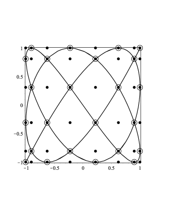
Figure 1. Lissajous curve $\gamma_{7,5}$; points of ${\rm LC}_{7,5}$ (big circles); points of the tensor product Chebyshev grid $\left\{(x_{i},y_{j}):i=0,\dots,7,\,j=0,\dots,5\right\}$ (small solid circles).

Proposition 3.1.

(See [10]). Let $({m,n})\in{\mathcal{N}}^{2}$. The set ${\rm LC}_{m,n}$ contains $(m+1)(n+1)/2$ distinct points and can be represented in the following form

$${\rm LC}_{m,n}=\left\{(x_{i},y_{j}):(i,j)\in{\mathcal{I}}_{m,n}\right\},$$

where

$${\mathcal{I}}_{m,n}=\left\{(i,j)\in{{\mathbb{Z}}}_{+}^{2}:i=0,\dots,m,\,j=0,\dots,n,\,i+j=0\pmod{2}\right\}.$$

Further, to study the interpolation problem on ${\rm LC}_{m,n}$, we need to introduce some additional notations. Let

$$C_{n}(x)=\cos(n\arccos x)$$

be the Chebyshev polynomial of the first kind. The normalized Chebyshev polynomial is defined by

$$\hat{C}_{n}(x)=\left\{\begin{array}[]{ll}1,&\hbox{$n=0$,}\\ \sqrt{2}C_{n}(x),&\hbox{$n\neq 0$.}\end{array}\right.$$

A proper set of polynomials for interpolation on ${\rm LC}_{m,n}$ is given by

$$\Pi_{m,n}^{\mathcal{L}}={\rm span}\{C_{k}(x)C_{l}(y)\,:\,(k,l)\in\Gamma_{m,n}^{\mathcal{L}}\},$$

where

$${\Gamma}_{m,n}^{\mathcal{L}}=\left\{(i,j)\in{{\mathbb{Z}}}_{+}^{2}:\frac{i}{m}+\frac{j}{n}<1\right\}\cup\{(0,n)\}.$$

To construct the Lagrange interpolation polynomial corresponding to the sets ${\rm LC}_{m,n}$ and $\Pi_{m,n}^{\mathcal{L}}$, we will use the following weights

(3.2) $${\lambda}_{i,j}:=\left\{\begin{array}[]{ll}\displaystyle 1/{(2mn)},&\hbox{$(x_{i},y_{j})$ is a vertex point of $J^{2}$,}\\ \displaystyle 1/(mn),&\hbox{$(x_{i},y_{j})$ is an edge point of $J^{2}$,}\\ \displaystyle 2/(mn),&\hbox{$(x_{i},y_{j})$ is an interior point of $J^{2}$.}\end{array}\right.$$

Let us present two basic theorems for our further consideration.

Theorem 3.1.

(See [10]). For $f\in B(J^{2})$, the unique solution of the interpolation problem

$${\mathcal{L}}_{m,n}(f)(x_{k},y_{l})=f(x_{k},y_{l}),\quad(x_{k},y_{l})\in{\rm LC}_{m,n},$$

in the space $\Pi_{n,m}^{\mathcal{L}}$ is given by the polynomial

(3.3) $${\mathcal{L}}_{m,n}f(x,y)=\sum_{(k,l)\in{\mathcal{I}}_{m,n}}f(x_{k},y_{l})\ell_{m,n}(x,y;x_{k},y_{l}),$$

where

(3.4) $$\begin{split}\ell_{m,n}(x,y;x_{k},y_{l})&={\lambda}_{k,l}\left(\sum_{(i,j)\in\Gamma_{m,n}^{\mathcal{L}}}\hat{C}_{i}(x_{k})\hat{C}_{j}(y_{l})\hat{C}_{i}(x)\hat{C}_{j}(y)-\frac{1}{2}\hat{C}_{n}(y_{l})\hat{C}_{n}(y)\right).\end{split}$$

These polynomials form the fundamental polynomials of Lagrange interpolation in the space $\Pi_{m,n}^{\mathcal{L}}$ with respect to the point set ${\rm LC}_{m,n}$, i.e. $\ell_{m,n}(x_{k^{\prime}},y_{l^{\prime}};x_{k},y_{l})=\delta_{(k,l),(k^{\prime},l^{\prime})}.$

The next theorem was obtained in [7]. In what follows for $r,s\in{{\mathbb{Z}}}_{+}$, we denote

$$f^{(r,s)}(x,y)=\frac{\partial^{r+s}f}{\partial x^{r}\partial y^{s}}(x,y).$$

Theorem 3.2.

For $f\in C(J^{2})$ and $(m,n)\in{\mathcal{N}}^{2}$, we have

$$\|f-{\mathcal{L}}_{m,n}f\|_{L_{\infty}(J^{2})}\leq C\log(m+1)\log(n+1)E(f,\Pi_{m,n}^{\mathcal{L}})_{L_{\infty}(J^{2})},$$

where $C$ is some absolute constant. In particular, if $f^{(r,0)},f^{(0,s)}\in C(J^{2})$ for some $r,s\in{{\mathbb{Z}}}_{+}$, then

$$\begin{split}\|f-&{\mathcal{L}}_{m,n}(f)\|_{L_{\infty}(J^{2})}\\ &\leq C_{r,s}\log(m+1)\log(n+1)\left({m^{-r}}{\omega}^{(1)}(f^{(r,0)},{m^{-1}})_{\infty}+{n^{-s}}{\omega}^{(2)}(f^{(0,s)},{n^{-1}})_{\infty}\right),\end{split}$$

where

$${\omega}^{(1)}(f,{\delta})_{\infty}=\sup_{|h|\leq 1-{\delta}}\|f(\cdot+h,\cdot)-f\|_{\infty},$$

$${\omega}^{(2)}(f,{\delta})_{\infty}=\sup_{|h|\leq 1-{\delta}}\|f(\cdot,\cdot+h)-f\|_{\infty}$$

are the partial moduli of continuity by the first and second variables, correspondingly.

4. Main results

Our goal is to obtain analogues of Theorem 3.2 in the weighted $L_{p}$-spaces. We say that a real bivariate function $f:D\to{\mathbb{R}}^{2}$ belongs to the weighted space $L_{p,u}(D)$, $1\leq p<\infty$, with the weight $u(x,y)\geq 0$ if

$$\|f\|_{L_{p,u}(D)}=\left(\int_{D}|f(x,y)u(x,y)|^{p}{\rm d}x{\rm d}y\right)<\infty.$$

We denote the Chebyshev-type weight $w$ in the case $D=J^{2}=[-1,1]^{2}$ by

$$w(x,y)=\frac{1}{\left(\sqrt{1-x^{2}}\sqrt{1-y^{2}}\right)^{\frac{1}{p}}}.$$

In the one-dimensional case, the function $w$ has the same meaning, i.e. $w(x)=(1-x^{2})^{-1/(2p)}$. In what follows, if $u\equiv 1$, then we denote $\|f\|_{L_{p}(D)}=\|f\|_{L_{p,u}(D)}$.

Everywhere below, $c_{p}$ and $C_{p}$ denote some positive constants depending only on $p$.

From Theorem 2.2 and Lemma 5.1 in Section 5 below, we directly obtain the following quite standard result.

Theorem 4.1.

Let $f\in B(J^{2})$, $1\leq p<\infty$, and $(m,n)\in{\mathcal{N}}^{2}$. Then

$$\|f-{\mathcal{L}}_{m,n}f\|_{L_{p,w}(J^{2})}\leq C_{p}K_{p}({m,n})\widetilde{E}(f,\Pi_{m,n}^{\mathcal{L}})_{L_{p,w}(J^{2})},$$

where

(4.1) $$K_{p}(m,n)=\left\{\begin{array}[]{ll}\log(m+1)\log(n+1),&\hbox{$p=1$,}\\ 1,&\hbox{$1<p<\infty$.}\end{array}\right.$$

The error of the best one-sided approximation $\widetilde{E}(f,\Pi_{m,n}^{\mathcal{L}})_{L_{p,w}(J^{2})}$ is a rather specific quantity, for which, in fact, it is difficult to find effective estimates via more classical objects. In the case of standard polynomial spaces, some estimates of the error of the best one-sided approximation can be found in [26], [15], [14]. For example, it is well-known that in the one-dimensional case for any periodic function $f$ of bounded variation on ${{\mathbb{T}}}\simeq[-\pi,\pi)$ and $1\leq p<\infty$, one has (see Lemma 5.8)

(4.2) $$\widetilde{E}(f,{\mathcal{T}}_{n})_{L_{p}({{\mathbb{T}}})}=\mathcal{O}({n^{-1/p}}),$$

where ${\mathcal{T}}_{n}$ is the set of all univariate real trigonometric polynomials of order at most $n$. Note that (4.2) implies some well-known estimates of the error of approximation of $f$ by the classical Lagrange interpolation polynomials on equidistant nodes [25] (see also [22], [23]).

We do not know if it is possible to obtain similar estimates in the multivariate case which can be used together with Theorem 4.1 to obtain efficient estimates of $\|f-{\mathcal{L}}_{m,n}f\|_{L_{p,w}(J^{2})}$. In this paper, instead of utilizing Theorem 4.1, we apply another approach based on Theorem 2.1. To introduce this approach, we need to recall some notation.

Let $BV(I)$, $I=[a,b]$, be the set of all real-valued functions $f:I\to{\mathbb{R}}$ with bounded variation on $I$. Recall that $f\in BV(I)$ if

$$V_{I}(f)=\sup_{a\leq\xi_{1}<\dots<\xi_{n}\leq b}\sum_{k=1}^{n-1}|f(\xi_{k+1})-f(\xi_{k})|<\infty.$$

A real-valued bivariate function $f\,:\,I^{2}\to{\mathbb{R}}$ is said to be of bounded variation on $I^{2}$ in the sense of Hardy-Krause (see [1]) if $f(\cdot,y),f(x,\cdot)\in BV(I)$ for some fixed $x,y\in I$ and if

$$H_{I^{2}}(f)=\sup_{\pi_{1},\pi_{2}}\sum_{k=1}^{m-1}\sum_{l=1}^{n-1}|{\Delta}f(\xi_{k},\eta_{l})|<\infty,$$

where

$${\Delta}f(\xi_{k},\eta_{l})=f(\xi_{k+1},\eta_{l+1})-f(\xi_{k+1},\eta_{l})-f(\xi_{k},\eta_{l+1})+f(\xi_{k},\eta_{l})$$

and

$$\pi_{1}:a\leq\xi_{1}<\dots<\xi_{m}\leq b,$$

$$\pi_{2}:a\leq\eta_{1}<\dots<\eta_{n}\leq b$$

are arbitrary decompositions of $I$. The class of such functions $f$ we denote by $HBV(I^{2})$. Other classes of functions of multivariate bounded variation as well as their relation to the class $HBV(I^{2})$ can be found, e.g., in [1].

Note that if $f\in HBV(I^{2})$, then $f(\cdot,y)$, $f(x,\cdot)\in BV(I)$ for any fixed $x,y\in I$. In what follows the values

$$V_{1,I}(f)(y)\quad\text{and}\quad V_{2,I}(f)(x)$$

are defined as the total variations of $f(\cdot,y)$ and $f(x,\cdot)$ on $I$. Note that for $f\in HBV(I^{2})$ we also have $V_{1,I}(f)$, $V_{2,I}(f)\in BV(I)$ (see [1]). Hence, $\sup_{y\in I}V_{1,I}(f)(y)$ and $\sup_{x\in I}V_{2,I}(f)(x)$ are finite.

Denote

$$\widetilde{D}^{(r,s)}f(x,y)=\left\{\frac{\partial^{r+s}}{\partial^{r}\!\phi\,\partial^{s}\psi}f(\cos\phi,\cos\psi)\right\}_{\phi=\arccos x,\,\psi=\arccos y}.$$

The following theorem is one of the main results of this paper.

Theorem 4.2.

Let $f\in B(J^{2})$, $1\leq p<\infty$, $r,s\in{{\mathbb{Z}}}_{+}$, and $(m,n)\in{\mathcal{N}}^{2}$. If $\widetilde{D}^{(r,s)}f\in HBV(J^{2})$, then

$$\begin{split}\|f-{\mathcal{L}}_{m,n}f&\|_{L_{p,w}(J^{2})}\leq CK_{p}(m,n)\bigg{(}{m^{-\frac{1}{p}-r}}\|V_{1,J}(\widetilde{D}^{(r,0)}f)\|_{L_{p,w}(J)}\\ &+{n^{-\frac{1}{p}-s}}\|V_{2,J}(\widetilde{D}^{(0,s)}f)\|_{L_{p,w}(J)}+m^{-\frac{1}{p}-r}n^{-\frac{1}{p}-s}H_{J^{2}}(\widetilde{D}^{(r,s)}f)\bigg{)},\end{split}$$

where the constant $C$ does not depend on $m$, $n$, and $f$.

Denote ${\varphi}(t)=\sqrt{1-t^{2}}$, ${\varphi}_{1}(x,y)={\varphi}(x)$, and ${\varphi}_{2}(x,y)={\varphi}(y)$.

Corollary 4.1.

Let $f\in B(J^{2})$, $1\leq p<\infty$, $r,s\in\{0,1\}$, and $(m,n)\in{\mathcal{N}}^{2}$. If ${\varphi}_{1}^{r}{\varphi}_{2}^{s}f^{(r,s)}\in HBV(J^{2})$, then

$$\begin{split}\|f-{\mathcal{L}}_{m,n}f&\|_{L_{p,w}(J^{2})}\leq CK_{p}(m,n)\bigg{(}{m^{-\frac{1}{p}-r}}\|V_{1,J}({\varphi}_{1}^{r}f^{(r,0)})\|_{L_{p,w}(J)}\\ &+{n^{-\frac{1}{p}-s}}\|V_{2,J}({\varphi}_{2}^{s}f^{(0,s)})\|_{L_{p,w}(J)}+m^{-\frac{1}{p}-r}n^{-\frac{1}{p}-s}H_{J^{2}}({\varphi}_{1}^{r}{\varphi}_{2}^{s}f^{(r,s)})\bigg{)},\end{split}$$

where the constant $C$ does not depend on $m$, $n$, and $f$.

Sharper results can be obtained in terms of moduli of smoothness and the errors of the best approximation of functions by algebraic polynomials. To formulate such results, let us recall some notations.

Denote

$$\Delta_{h}^{\nu}(f,x)=\left\{\begin{array}[]{ll}\displaystyle{\sum_{i=1}^{\nu}}\binom{\nu}{i}(-1)^{\nu-i}f(x+(i-\nu/2)h),&\hbox{$x\pm\nu h/2\in J$,}\\ \displaystyle 0,&\hbox{otherwise.}\end{array}\right.$$

The weighted Ditzian-Totik modulus of smoothness of $f\in L_{p,u}(J)$ of order $\nu\in{{\mathbb{N}}}$ and step $t>0$ is defined by

(4.3) $$\begin{split}{\omega}_{\nu}^{\varphi}(f,t)_{p,u}=\sup_{0<h\leq t}&\|u{\Delta}_{h{\varphi}}^{\nu}f\|_{L_{p}[-1+t^{*},1-t^{*}]}\\ &+\sup_{0<h\leq t}\|u\overrightarrow{{\Delta}}_{h}^{\nu}f\|_{L_{p}[-1,-1+At^{*}]}+\sup_{0<h\leq t}\|u\overleftarrow{{\Delta}}_{h}^{\nu}f\|_{L_{p}[1-At^{*},1]},\end{split}$$

where $t^{*}=2\nu^{2}t^{2}$, $A$ is an absolute constant, and the forward and backward $\nu$th differences are given by

$$\overrightarrow{{\Delta}}_{h}^{\nu}f(x)={\Delta}_{h}^{\nu}(f,x+\nu h/2),\quad\overleftarrow{{\Delta}}_{h}^{\nu}f(x)={\Delta}_{h}^{\nu}(f,x-\nu h/2)$$

(for details see [9, p. 218]).

In our work, we mainly deal with the following analogue of (4.3) given by

(4.4) $${\omega}_{\nu,{\alpha}}^{\varphi}(f,t)_{p}=\sup_{0\leq h\leq t}\|\mathcal{W}_{\nu h}^{\alpha}{\Delta}_{h{\varphi}}^{\nu}(f,\cdot)\|_{L_{p}(J)},$$

where

$$\mathcal{W}_{\delta}(x)=\left(\left(1-x-\frac{{\delta}{\varphi}(x)}{2}\right)\left(1+x-\frac{{\delta}{\varphi}(x)}{2}\right)\right)^{\frac{1}{2}}.$$

The modulus (4.4) has been recently introduced in [17]. It is known (see [18]) that at least for ${\alpha}\in{{\mathbb{N}}}$ the modulus (4.4) is equivalent to the weighted Ditzian-Totik modulus of smoothness (4.3) with $u={\varphi}^{\alpha}$.

Let us extend the modulus of smoothness (4.4) to the bivariate case. For this we denote $\mathcal{W}_{\delta}^{1}(x,y)=\mathcal{W}_{\delta}(x)$ and $\mathcal{W}_{\delta}^{2}(x,y)=\mathcal{W}_{\delta}(y)$. Let also $w_{1}(x,y)=w(x)$ and $w_{2}(x,y)=w(y)$.

For an admissible $f\,:\,J^{2}\to{\mathbb{R}}$, the partial moduli of smoothness related to (4.4) are defined by

$${\omega}_{\nu,{\alpha}}^{{\varphi},j}(f,t)_{p}=\sup_{0\leq h\leq t}\|\mathcal{W}_{\nu h}^{{\alpha},j}{\Delta}_{h{\varphi}_{j}}^{\nu,j}(f,\cdot)\|_{L_{p,w_{i}}(J^{2})},\quad i,j=1,2,\quad i\neq j,$$

where ${\Delta}_{h{\varphi}_{j}}^{\nu,j}={\Delta}_{h{\varphi}_{j}e_{j}}^{\nu}$ and $e_{1}=(1,0)$, $e_{2}=(0,1)$. The corresponding mixed modulus of smoothness is given by

$${\omega}_{\nu,{\alpha}_{1},{\alpha}_{2}}^{{\varphi}}(f,t_{1},t_{2})_{p}=\sup_{0\leq h_{j}\leq t_{j},\,j=1,2}\|\mathcal{W}_{\nu h_{1}}^{{\alpha}_{1},1}\mathcal{W}_{\nu h_{2}}^{{\alpha}_{2},2}{\Delta}_{h_{1}{\varphi}_{1}}^{\nu,1}{\Delta}_{h_{2}{\varphi}_{2}}^{\nu,2}(f,\cdot)\|_{L_{p}(J^{2})}.$$

Now we are ready to formulate a result which gives a refinement of Theorem 4.2 in the case of smooth functions. In what follows, we denote the set of all (locally) absolutely continuous functions on $[a,b]$ by $AC([a,b])$ ($AC_{\rm loc}([a,b])$).

Theorem 4.3.

Let $f\in B(J^{2})$, $1\leq p<\infty$, $r,s\in{{\mathbb{N}}}$, $\nu\in{{\mathbb{N}}}$, and $(m,n)\in{\mathcal{N}}^{2}$. Suppose $f^{(r-1,0)}(\cdot,y)$ and $f^{(r,s-1)}(\cdot,y)$ or $f^{(0,s-1)}(x,\cdot)$ and $f^{(r-1,s)}(x,\cdot)$ belong to $AC_{\rm loc}(J)$ for a.e. $x,y\in J$. If, in addition, ${\varphi}_{1}^{r}f^{(r,0)}$, ${\varphi}_{2}^{s}f^{(0,s)}$, ${\varphi}_{1}^{r}{\varphi}_{2}^{s}f^{(r,s)}\in L_{p,w}(J^{2})$, and $m>r$, $n>s$, then

$$\begin{split}\|f-&{\mathcal{L}}_{m,n}f\|_{L_{p,w}(J^{2})}\leq CK_{p}(m,n)\Bigg{(}{m^{-r}}{\omega}_{\nu,r-1/p}^{{\varphi},1}\left(f^{(r,0)},m^{-1}\right)_{p}\\ &+{n^{-s}}{\omega}_{\nu,s-1/p}^{{\varphi},2}\left(f^{(0,s)},n^{-1}\right)_{p}+{m^{-r}}n^{-s}{\omega}_{\nu,r-1/p,s-1/p}^{{\varphi}}\left(f^{(r,s)},m^{-1},n^{-1}\right)_{p}\Bigg{)},\end{split}$$

where the constant $C$ does not depend on $m$, $n$, and $f$.

Remark 4.1.

Note that Theorem 4.2 is valid also for discontinuous functions of bounded variation while in Theorem 4.3 we have to require the existence of partial and mixed derivatives of at least first order. We have a similar situation in Theorem 4.4 and Theorem 4.5 stated below.

It is also possible to obtain estimates of the error of approximation of functions $f$ by interpolation polynomials ${\mathcal{L}}_{m,n}f$ without using mixed moduli of smoothness, mixed derivatives, and the notion of bounded variation in the sense of Hardy-Krause. To formulate such results we need some additional notation.

Let $\mathcal{P}_{n}$ be the space of all real-valued univariate algebraic polynomials of degree at most $n$. In what follows, for simplicity, we denote

$$E_{n}^{\mathcal{P}}(f)_{L_{p,u}(J)}=E(f,\mathcal{P}_{n})_{L_{p,u}(J)}.$$

Let also

$$E_{m,\infty}^{\mathcal{P}}(f)_{L_{p,u}(J^{2})}=E(f,{\mathcal{P}}_{m,\infty}(L_{p,u}))_{L_{p,u}(J^{2})},$$

where ${\mathcal{P}}_{m,\infty}(L_{p,u})$ is a class of functions $g$ such that $g\in L_{p,u}(J^{2})$ and $g$ is an algebraic polynomial of degree at most $m$ in the first variable. By analogy, we define the class ${\mathcal{P}}_{\infty,n}(L_{p,u})$ and

$$E_{\infty,n}^{\mathcal{P}}(f)_{L_{p,u}(J^{2})}=E(f,{\mathcal{P}}_{\infty,n}(L_{p,u}))_{L_{p,u}(J^{2})}.$$

In what follows, for a sequence $\{a_{k}\}_{k\in\mathcal{I}_{n}}$, $\mathcal{I}_{n}=\{0,1,\dots,n-1\}$, of numbers, we denote

$$\|\{a_{k}\}\|_{\widetilde{\ell}_{p}^{n}}=\left(\frac{1}{n}\sum_{k=0}^{n-1}|a_{k}|^{p}\right)^{\frac{1}{p}}.$$

The following result is a counterpart of Theorem 4.3 for the errors of the best approximation. Recall that the points $x_{k}$ and $y_{l}$ are given by (3.1).

Theorem 4.4.

Let $f\in B(J^{2})$, $1\leq p<\infty$, $r,s\in{{\mathbb{N}}}$, and $(m,n)\in{\mathcal{N}}^{2}$. Suppose $f^{(r-1,0)}(\cdot,y)$, $f^{(0,s-1)}(x,\cdot)\in AC_{\rm loc}(J)$ for a.e. $x,y\in J$. If, in addition, ${\varphi}_{1}^{r}f^{(r,0)}\in L_{p,w}(J^{2})$ and ${\varphi}_{2}^{s}f^{(0,s)}(x_{k},\cdot)\in L_{p,w}(J)$ for all $k\in\mathcal{I}_{6m}$ and $m>r$, $n>s$, then

$$\begin{split}\|f-{\mathcal{L}}_{m,n}f\|_{L_{p,w}(J^{2})}\leq CK_{p}(m,n)\Big{(}m^{-r}&E_{m-r,\infty}^{\mathcal{P}}(f^{(r,0)})_{L_{p,{\varphi}_{1}^{r}w}(J^{2})}\\ &+n^{-s}\|\{E_{n-s}^{\mathcal{P}}(f^{(0,s)}(x_{k},\cdot))_{L_{p,{\varphi}_{2}^{s}w}(J)}\}\|_{\widetilde{\ell}_{p}^{6m}}\Big{)},\end{split}$$

where the constant $C$ does not depend on $m$, $n$, and $f$.

Remark 4.2.

The result symmetric to Theorem 4.4 has the following form: If we suppose in Theorem 4.4 that ${\varphi}_{2}^{s}f^{(0,s)}\in L_{p,w}(J^{2})$ and ${\varphi}_{1}^{s}f^{(r,0)}(\cdot,y_{k})\in L_{p,w}(J)$ for all $k\in\mathcal{I}_{6n}$, then

$$\begin{split}\|f-{\mathcal{L}}_{m,n}f\|_{L_{p}(J^{2})}\leq CK_{p}(m,n)\Big{(}n^{-s}&E_{\infty,{n-s}}^{\mathcal{P}}(f^{(0,s)})_{L_{p,{\varphi}_{2}^{s}w}(J^{2})}\\ &+m^{-r}\|\{E_{m-r}^{\mathcal{P}}(f^{(r,0)}(\cdot,y_{k}))_{L_{p,{\varphi}_{1}^{r}w}(J)}\}\|_{\widetilde{\ell}_{p}^{6n}}\Big{)},\end{split}$$

where the constant $C$ does not depend on $m$, $n$, and $f$.

For not necessarily smooth functions, we obtain the following analogues of Theorem 4.2 in terms of the classical bounded variation.

Theorem 4.5.

Let $f\in B(J^{2})$, $1\leq p<\infty$, $r,s\in{{\mathbb{Z}}}_{+}$, and $(m,n)\in{\mathcal{N}}^{2}$. Suppose that $\widetilde{D}^{(r,0)}f(\cdot,y)\in BV(J)$ for a.e. $y\in J$ and $\widetilde{D}^{(0,s)}f(x_{k},\cdot)\in BV(J)$ for all $k\in{\mathcal{I}}_{6m}$. If, in addition, $V_{1,J}(\widetilde{D}^{(r,0)}f)\in L_{p,w}(J)$, then

$$\begin{split}\|f-&{\mathcal{L}}_{m,n}f\|_{L_{p,w}(J^{2})}\\ &\leq CK_{p}(m,n)\left({m^{-r-1/p}}\|V_{1,J}(\widetilde{D}^{(r,0)}f)\|_{L_{p,w}({{\mathbb{T}}})}+{n^{-s-1/p}}\|\{V_{2,J}(\widetilde{D}^{(0,s)}f(x_{k},\cdot))\}\|_{\widetilde{\ell}_{p}^{6m}}\right),\end{split}$$

where the constant $C$ does not depend on $m$, $n$, and $f$.

Remark 4.3.

The result symmetric to Theorem 4.5 has the following form: If we suppose in Theorem 4.5 that $\widetilde{D}^{(0,s)}f(x,\cdot)\in BV(J)$ for a.e. $x\in J$ and $\widetilde{D}^{(r,0)}f(\cdot,y_{k})\in BV(J)$ for all $k\in{\mathcal{I}}_{6n}$, and, in addition, $V_{2,J}(\widetilde{D}^{(0,s)}f)\in L_{p,w}(J)$, then

$$\begin{split}\|f-&{\mathcal{L}}_{m,n}f\|_{L_{p,w}(J^{2})}\\ &\leq CK_{p}(m,n)\left({n^{-s-1/p}}\|V_{2,J}(\widetilde{D}^{(0,s)}f)\|_{L_{p,w}({{\mathbb{T}}})}+{m^{-r-1/p}}\|\{V_{1,J}(\widetilde{D}^{(r,0)}f(\cdot,y_{l}))\}\|_{\widetilde{\ell}_{p}^{6n}}\right),\end{split}$$

where the constant $C$ does not depend on $m$, $n$, and $f$.

5. Proof of the main results

5.1. Marcinkiewicz-Zygmund type inequalities

Let us start from the MZ type inequality for algebraic polynomials $P$ from $\Pi_{m,n}^{\mathcal{L}}$.

Lemma 5.1.

Let $1\leq p<\infty$ and $P\in\Pi_{m,n}^{\mathcal{L}}$. Then

(5.1) $$c_{p}\left(\sum_{(k,l)\in{\mathcal{I}}_{m,n}}{\lambda}_{k,l}|P(x_{k},y_{l})|^{p}\right)^{\frac{1}{p}}\leq\|P\|_{L_{p,w}(J^{2})},$$

(5.2) $$\|P\|_{L_{p,w}(J^{2})}\leq C_{p}K_{p}(m,n)\left(\sum_{(k,l)\in{\mathcal{I}}_{m,n}}{\lambda}_{k,l}|P(x_{k},y_{l})|^{p}\right)^{\frac{1}{p}},$$

where $\lambda_{k,l}$ and $K_{p}(m,n)$ are given by (3.2) and (4.1), correspondingly.

Proof.

The proof of (5.1) for all $1\leq p<\infty$ as well as the proof of (5.2) in the case $1<p<\infty$ one can find in [10]. Let us consider (5.2) in the case $p=1$. By (3.3), we get

(5.3) $$\|P\|_{L_{1,w}(J^{2})}\leq\sum_{(k,l)\in{\mathcal{I}}_{m,n}}|P(x_{k},y_{l})|\|\ell_{m,n}(\cdot,\cdot;x_{k},y_{l})\|_{L_{1,w}(J^{2})}.$$

At the same time, from [10] (see also [7]) it follows

(5.4) $$\sup_{(x,y)\in J^{2}}\|\ell_{m,n}(\cdot,\cdot;x,y)\|_{L_{1,w}(J^{2})}\leq C(mn)^{-1}\log(m+1)\log(n+1),$$

where $C$ is some absolute constant.

Combining (5.3) and (5.4), we proved the lemma. ∎

Now let us consider a trigonometric analogue of Lemma 5.1 for the following bivariate trigonometric polynomials given by

$${\mathcal{T}}_{m,n}^{\mathcal{L}}={\rm span}\{\cos(k\phi)\cos(l\psi)\,:\,(k,l)\in\Gamma_{m,n}^{\mathcal{L}}\}.$$

Lemma 5.2.

Let $1\leq p<\infty$ and $T\in{\mathcal{T}}_{m,n}^{\mathcal{L}}$. Then

$$\|T\|_{L_{p}({{\mathbb{T}}}^{2})}\leq C_{p}K_{p}(m,n)\left(\frac{1}{mn}\sum_{(k,l)\in{\mathcal{I}}_{m,n}}\Big{|}T\Big{(}\frac{\pi k}{m},\frac{\pi l}{n}\Big{)}\Big{|}^{p}\right)^{\frac{1}{p}}.$$

Proof.

We only need to apply the standard trigonometric substitution $x=\cos\phi$, $y=\cos\psi$ to the inequality (5.2) and to take into account that $T$ is an even polynomial in each variable. ∎

For application of Theorem 2.1, we need the following polynomial set

$${\mathcal{T}}_{m,n}^{\prime}=\operatorname{span}\{\cos(k\phi)\cos(l\psi)\,:\,(k,l)\in{\mathcal{I}}_{m,n}^{\prime}\},$$

where the index set is given by

$${{\mathcal{I}}}_{m,n}^{\prime}=\left\{(i,j)\in{{\mathbb{Z}}}_{+}^{2}:\begin{array}[]{ccc}i=0,\dots,6m-1\\ j=0,\dots,6n-1\end{array}\right\}.$$

Lemma 5.3.

Let $1\leq p<\infty$ and $T\in{\mathcal{T}}_{m,n}^{\prime}$. Then

$$c_{p}\left(\frac{1}{36mn}\sum_{(k,l)\in{\mathcal{I}}_{m,n}^{\prime}}\Big{|}T\Big{(}\frac{\pi k}{3m},\frac{\pi l}{3n}\Big{)}\Big{|}^{p}\right)^{\frac{1}{p}}\leq\|T\|_{L_{p}({{\mathbb{T}}}^{2})}.$$

Proof.

The proof easily follows from the well-known one-dimensional result, see, e.g., [28]:

(5.5) $$\bigg{(}\frac{1}{6n}\sum_{k=0}^{6n-1}\Big{|}T\Big{(}\frac{\pi k}{3n}\Big{)}\Big{|}^{p}\bigg{)}^{\frac{1}{p}}\leq C_{p}\|T\|_{L_{p}({{\mathbb{T}}})},\quad T\in{\mathcal{T}}_{6n},$$

where ${\mathcal{T}}_{n}$ is the set of all real-valued univariate trigonometric polynomials of order at most $n$. ∎

5.2. Weighted averaged moduli of smoothness

The following weighted Ditzian-Totik modulus of smoothness of $f\in L_{p,u}(J)$ was considered in [9, see (6.1.9)]

(5.6) $$\begin{split}{\omega}_{\nu}^{*{\varphi}}(f,t)_{p,u}=&\left(\frac{1}{t}\int_{0}^{t}\int_{-1+t^{*}}^{1-t^{*}}|u(x){\Delta}_{\tau{\varphi}}^{\nu}(f,x)|^{p}{\rm d}x{\rm d}\tau\right)^{\frac{1}{p}}\\ &+\left(\frac{1}{t^{*}}\int_{0}^{t^{*}}\int_{-1}^{-1+At^{*}}|u(x)\overrightarrow{{\Delta}}_{\tau}^{\nu}(f,x)|^{p}{\rm d}x{\rm d}\tau\right)^{\frac{1}{p}}\\ &+\left(\frac{1}{t^{*}}\int_{0}^{t^{*}}\int_{1-At^{*}}^{1}|u(x)\overleftarrow{{\Delta}}_{\tau}^{\nu}(f,x)|^{p}{\rm d}x{\rm d}\tau\right)^{\frac{1}{p}}\end{split}$$

(recall that $t^{*}=2\nu^{2}t^{2}$ and $A$ is some absolute constant).

For ${\delta}>0$, we denote

$$\begin{split}\mathcal{D}_{\delta}=\left\{x\in{\mathbb{R}}\,:\,1-\frac{{\delta}{\varphi}(x)}{2}\geq|x|\right\}\setminus\{\pm 1\}=\left\{|x|\leq\frac{4-{\delta}^{2}}{4+{\delta}^{2}}\right\}.\end{split}$$

In [18], in connection with the modulus (4.4), it was introduced a ”modification”  of the averaged modulus of smoothness (5.6). For $f\in L_{p,{\varphi}^{\alpha}}(J)$, it is defined by

(5.7) $${\omega}_{\nu,{\alpha}}^{*{\varphi}}(f,t)_{p}=\left(\frac{1}{t}\int_{0}^{t}\|\mathcal{W}_{\nu\tau}^{{\alpha}}{\Delta}_{\tau{\varphi}}^{\nu}(f,\cdot)\|_{L_{p}(\mathcal{D}_{\nu\tau})}^{p}{\rm d}\tau\right)^{\frac{1}{p}}.$$

In contrast to (5.6), this modulus of smoothness is more convenient for the goal of this paper.

We have the following inequalities for the moduli of smoothness introduced above.

Lemma 5.4.

Let $\nu\in{{\mathbb{N}}}$, ${\alpha}>0$, and ${\varphi}^{\alpha}f\in L_{p}(J)$, $1\leq p<\infty$. Then

(5.8) $${\omega}_{\nu}^{\varphi}(f,t)_{p,{\varphi}^{\alpha}}\leq c{\omega}_{\nu}^{*{\varphi}}(f,t)_{p,{\varphi}^{\alpha}}\leq C{\omega}_{\nu,{\alpha}}^{*{\varphi}}(f,t)_{p}\leq C{\omega}_{\nu,{\alpha}}^{{\varphi}}(f,t)_{p},$$

where the constants $c$ and $C$ do not depend on $t$ and $f$.

Proof.

The scheme of proving the first inequality in (5.8) can be found in [9, pp. 56–57]. The second inequality can be shown analogously to the proof of Lemma 6.1 in [18]. The third inequality is obvious. ∎

Now let us introduce bivariate analogues of the modulus of smoothness (5.7).

For $f\,:\,J^{2}\to{\mathbb{R}}$ and $i,j=1,2$, where $i\neq j$, we define the partial averaged modulus of smoothness by

$${\omega}_{\nu,{\alpha}}^{*{\varphi},j}(f,t)_{p}=\left(\frac{1}{t}\int_{0}^{t}{\rm d}\tau\int_{\mathcal{D}_{\nu\tau}}{\rm d}x_{j}\int_{-1}^{1}|\mathcal{W}_{\nu\tau}^{{\alpha}}(x_{j}){\Delta}_{\tau{\varphi}(x_{j})}^{\nu,j}(f,x_{1},x_{2})|^{p}\frac{{\rm d}x_{i}}{\sqrt{1-x_{i}^{2}}}\right)^{\frac{1}{p}}.$$

A corresponding mixed averaged modulus of smoothness is given by

$$\begin{split}{\omega}_{\nu,{\alpha}_{1},{\alpha}_{1}}^{*{\varphi}}&(f,t_{1},t_{2})_{p}\\ &=\left(\frac{1}{t_{1}t_{2}}\int_{0}^{t_{1}}\int_{0}^{t_{2}}\|\mathcal{W}_{\nu\tau_{1}}^{{\alpha}_{1},1}\mathcal{W}_{\nu\tau_{2}}^{{\alpha}_{2},2}{\Delta}_{\tau_{1}{\varphi}_{1}}^{\nu,1}{\Delta}_{\tau_{2}{\varphi}_{2}}^{\nu,2}(f,\cdot)\|_{L_{p}(\mathcal{D}_{\nu\tau_{1}}\times\mathcal{D}_{\nu\tau_{2}})}^{p}{\rm d}\tau_{1}{\rm d}\tau_{2}\right)^{\frac{1}{p}}.\end{split}$$

5.3. Weighted error of the best approximation by algebraic polynomials

We will use the following Jackson-type inequalities for $E_{n}^{\mathcal{P}}(f)_{L_{p,u}(J)}$.

Lemma 5.5.

Let $0\leq r<\nu$, ${\alpha}>0$, $f^{(r-1)}$ be locally absolutely continuous in $(-1,1)$, and ${\varphi}^{{\alpha}+r}f^{(r)}\in L_{p}(J)$, $1\leq p<\infty$. Then

(5.9) $$E_{n}^{\mathcal{P}}(f)_{L_{p,{\varphi}^{\alpha}}(J)}\leq Cn^{-r}{\omega}_{\nu-r}^{\varphi}(f^{(r)},n^{-1})_{p,{\varphi}^{{\alpha}+r}},\quad n>r.$$

In particular,

(5.10) $$E_{n}^{\mathcal{P}}(f)_{L_{p,{\varphi}^{\alpha}}(J)}\leq Cn^{-r}E_{n-r}^{\mathcal{P}}(f^{(r)})_{L_{p,{\varphi}^{{\alpha}+r}}(J)},\quad n>r,$$

where the constant $C$ does not depend on $n$ and $f$.

Proof.

Inequality (5.9) can be found in [17]. The proof of (5.10) follows from [19, Theorem 1]. In particular, we have

$$E_{n}^{\mathcal{P}}(f)_{L_{p,{\varphi}^{\alpha}}(J)}=E_{n}^{\mathcal{P}}(f-P_{n})_{L_{p,{\varphi}^{\alpha}}(J)}\leq Cn^{-r}\|{\varphi}^{r}(f-P_{n})^{(r)}\|_{L_{p,{\varphi}^{\alpha}}(J)},$$

where we choose the polynomial $P\in{\mathcal{P}}_{n}$ such that

$$\|{\varphi}^{r+{\alpha}}(f^{(r)}-P_{n}^{(r)})\|_{L_{p}(J)}=E_{n-r}^{\mathcal{P}}(f^{(r)})_{L_{p,{\varphi}^{r+{\alpha}}}(J)}.$$

∎

5.4. De la Vallée-Poussin means

Let us consider the de la Vallée-Poussin means of Lagrange interpolation polynomials (see [27]). These means will play the role of an intermediate approximant $\mathcal{L}_{\bm{n}}^{\prime}$ in the application of Theorem 2.1.

We start form the one-dimensional case, in which de la Vallée-Poussin means are given by

(5.11) $${\mathcal{V}}_{n}f(\phi)={\mathcal{V}}_{n}(f,\phi)=\frac{1}{3n}\sum_{k=0}^{6n-1}f\left(t_{k}\right)K_{n}\left(\phi-t_{k}\right),\quad t_{k}=\frac{\pi k}{3n},$$

where

$$K_{n}(\phi)=\frac{1}{2}+\sum_{k=1}^{2n}\cos k\phi+\sum_{k=2n+1}^{4n-1}\frac{4n-k}{2n}\cos k\phi.$$

Recall some basic properties of ${\mathcal{V}}_{n}(f,\phi)$ (see [27]).

Lemma 5.6.

The following assertions hold:

1) $\deg{\mathcal{V}}_{n}f\leq 4n-1$;

2) ${\mathcal{V}}_{n}f\left(t_{k}\right)=f\left(t_{k}\right),\quad k=0,\dots,6n-1$;

3) ${\mathcal{V}}_{n}T(\phi)=T(\phi)$ for any $T\in{\mathcal{T}}_{2n}$.

Lemma 5.7.

Let $f\in B({{\mathbb{T}}})$, $1\leq p<\infty$, and $n\in{{\mathbb{N}}}$. Then

$$\|f-{\mathcal{V}}_{n}f\|_{L_{p}({{\mathbb{T}}})}\leq C_{p}\widetilde{E}(f,{\mathcal{T}}_{n})_{L_{p}({{\mathbb{T}}})}.$$

Proof.

Let $q_{n},Q_{n}\in{\mathcal{T}}_{n}$ be such that $q_{n}(t)\leq f(t)\leq Q_{n}(t)$ and $\|Q_{n}-q_{n}\|_{L_{p}({{\mathbb{T}}})}=\widetilde{E}(f,{\mathcal{T}}_{n})_{L_{p}({{\mathbb{T}}})}$. Similarly to (2.8) and (2.9), we derive

(5.12) $$\|f-{\mathcal{V}}_{n}f\|_{L_{p}({{\mathbb{T}}})}\leq\widetilde{E}(f,{\mathcal{T}}_{n})_{L_{p}({{\mathbb{T}}})}+\|q_{n}-{\mathcal{V}}_{n}f\|_{L_{p}({{\mathbb{T}}})}.$$

Next, using Lemma 5.6, item 3, the inequality

(5.13) $$\|{\mathcal{V}}_{n}f\|_{L_{p}({{\mathbb{T}}})}\leq C_{p}\left(\frac{1}{n}\sum_{k=0}^{6n-1}|f(t_{k})|^{p}\right)^{\frac{1}{p}},$$

which can be proved similarly to Theorem 3.2.3 in [20], and inequality (5.5), we obtain

(5.14) $$\begin{split}\|q_{n}-{\mathcal{V}}_{n}f\|_{L_{p}({{\mathbb{T}}})}&=\|{\mathcal{V}}_{n}(q_{n}-f)\|_{L_{p}({{\mathbb{T}}})}\leq C\left(\frac{1}{n}\sum_{k=0}^{6n-1}|q_{n}(t_{k})-f(t_{k})|^{p}\right)^{\frac{1}{p}}\\ &\leq C\left(\frac{1}{n}\sum_{k=0}^{6n-1}|q_{n}(t_{k})-Q_{n}(t_{k})|^{p}\right)^{\frac{1}{p}}\\ &\leq C\|q_{n}-Q_{n}\|_{L_{p}({{\mathbb{T}}})}=C\widetilde{E}(f,{\mathcal{T}}_{n})_{L_{p}({{\mathbb{T}}})}.\end{split}$$

Finally, combining (5.12) and (5.14), we proved the lemma. ∎

Lemma 5.8.

Let $f\in B({{\mathbb{T}}})$, $1\leq p<\infty$, and $n\in{{\mathbb{N}}}$.

1) If $f$ is an absolutely continuous function on ${{\mathbb{T}}}$ and $f^{\prime}\in L_{p}({{\mathbb{T}}})$, then

$$\|f-{\mathcal{V}}_{n}f\|_{L_{p}({{\mathbb{T}}})}\leq{C_{p}}{n^{-1}}{E}(f^{\prime},{\mathcal{T}}_{n})_{L_{p}({{\mathbb{T}}})}.$$

2) If $f\in BV({{\mathbb{T}}})$, then

$$\|f-{\mathcal{V}}_{n}f\|_{L_{p}({{\mathbb{T}}})}\leq{C_{p}}{n^{-\frac{1}{p}}}V_{{\mathbb{T}}}(f).$$

Proof.

The assertions of the lemma follow from Lemma 5.7 and the following two inequalities:

$$\widetilde{E}(f,{\mathcal{T}}_{n})_{L_{p}({{\mathbb{T}}})}\leq{C_{p}}{n^{-1}}{E}(f^{\prime},{\mathcal{T}}_{n})_{L_{p}({{\mathbb{T}}})},$$

$$\widetilde{E}(f,{\mathcal{T}}_{n})_{L_{p}({{\mathbb{T}}})}\leq{C_{p}}{n^{-\frac{1}{p}}}V_{{\mathbb{T}}}(f).$$

The first inequality can be found, e.g., in [26, Theorem 8.1]. The second one follows from [26, see Theorem 8.2 and the formula (7) on p. 10]. ∎

In what follows we denote

$$f^{*}(\phi)=f(\cos\phi).$$

Lemma 5.9.

Let $r,\nu\in{{\mathbb{N}}}$, $f^{(r-1)}$ be locally absolutely continuous on $(-1,1)$, and ${\varphi}^{r}f^{(r)}\in L_{p,w}(J)$, $1\leq p<\infty$. Then

(5.15) $$\|f^{*}-\mathcal{V}_{n}f^{*}\|_{L_{p}({{\mathbb{T}}})}\leq Cn^{-r}{\omega}_{\nu,r-1/p}^{*{\varphi}}(f^{(r)},n^{-1})_{p},\quad n>r,$$

where the constant $C$ does not depend on $n$ and $f$.

Proof.

A simple observation is that it is sufficient to derive (5.15) for functions $f$ with an absolutely continuous derivative $f^{(r-1)}$ on $[-1,1]$. Indeed, first we can prove (5.15) for the functions $f_{\rho}(x)=f(\rho x)$ and then to take limit as $\rho\to 1$ (see also [8, p. 260]).

Thus, by Lemma 5.8, we have

(5.16) $$\|f^{*}-\mathcal{V}_{n}f^{*}\|_{L_{p}({{\mathbb{T}}})}\leq Cn^{-1}E((f^{*})^{\prime},{\mathcal{T}}_{n})_{L_{p}({{\mathbb{T}}})}.$$

Let $P_{n-1}\in\mathcal{P}_{n-1}$ be such that

$$\|f^{\prime}-P_{n-1}\|_{L_{p,w{\varphi}}(J)}=E_{n-1}^{\mathcal{P}}(f^{\prime})_{L_{p,w{\varphi}}(J)}.$$

Then, using Lemma 5.5 and Lemma 5.4, we derive

(5.17) $$\begin{split}E((f^{*})^{\prime},{\mathcal{T}}_{n})_{L_{p}({{\mathbb{T}}})}&\leq\|\sin\phi f^{\prime}(\cos\phi)-\sin\phi P_{n-1}(\cos\phi)\|_{L_{p}({{\mathbb{T}}})}\\ &=\|(f^{\prime}-P_{n-1}){\varphi}\|_{L_{p,w}(J)}=E_{n-1}^{\mathcal{P}}(f^{\prime})_{L_{p,w{\varphi}}(J)}\\ &\leq Cn^{-r+1}{\omega}_{\nu}^{\varphi}(f^{(r)},n^{-1})_{p,w{\varphi}^{r}}\\ &\leq Cn^{-r+1}{\omega}_{\nu,r-1/p}^{*{\varphi}}(f^{(r)},n^{-1})_{p}.\end{split}$$

Combining (5.16) and (5.17), we get (5.15). ∎

Now let us consider the multidimensional analogue of (5.11). Let $f:{\mathbb{R}}^{2}\to{\mathbb{R}}$ be $2\pi$-periodic in each variable. We introduce the bivariate de la Vallée-Poussin type interpolation operator by

$${\mathcal{V}}_{m,n}f(\phi,\psi)={\mathcal{V}}_{m,n}(f,\phi,\psi)=\frac{1}{9mn}\sum_{(k,l)\in{{\mathcal{I}}}_{m,n}^{\prime}}f(\phi_{k},\psi_{l})K_{m}(\phi-\phi_{k})K_{n}(\psi-\psi_{l}),$$

where

$$\phi_{k}=\frac{\pi k}{3m},\quad\psi_{l}=\frac{\pi l}{3n},\quad k=0,\dots,6m-1,\quad l=0,\dots,6n-1.$$

We also need the following auxiliary operators:

$${\mathcal{V}}_{m,\infty}f(\phi,\psi)={\mathcal{V}}_{m,\infty}(f,\phi,\psi)={\mathcal{V}}_{m}(f(\cdot,\psi),\phi),$$

$${\mathcal{V}}_{\infty,n}f(\phi,\psi)={\mathcal{V}}_{\infty,n}(f,\phi,\psi)={\mathcal{V}}_{n}(f(\phi,\cdot),\psi).$$

It is easy to see that ${\mathcal{V}}_{m,n}(f,\phi,\psi)={\mathcal{V}}_{m,\infty}({\mathcal{V}}_{\infty,n}f,\phi,\psi)$.

In what follows, we pass from the algebraic case of functions on $J^{2}$ to the case of periodic functions on ${{\mathbb{T}}}^{2}\simeq[0,2\pi)^{2}$, by using the standard substitution

$$f^{*}(\phi,\psi)=f(\cos\phi,\cos\psi).$$

Everywhere below we also denote $I=[0,\pi)$.

Lemma 5.10.

Let $f\in B(J^{2})$, $1\leq p<\infty$, and $(m,n)\in{\mathcal{N}}^{2}$. Then

$$\begin{split}\|f-&{{\mathcal{L}}}_{m,n}f\|_{L_{p,w}(J^{2})}\\ &\leq C_{p}K_{p}(m,n)\left(\|f^{*}-{\mathcal{V}}_{\lfloor\frac{m}{8}\rfloor,\lfloor\frac{n}{8}\rfloor}f^{*}\|_{L_{p}({{\mathbb{T}}}^{2})}+\|f^{*}-{\mathcal{V}}_{m,n}f^{*}\|_{L_{p}({{\mathbb{T}}}^{2})}\right).\end{split}$$

Proof.

Consider the interpolation polynomial

$$\begin{split}{\mathcal{L}}_{m,n}^{\mathcal{T}}f^{*}(\phi,\psi)&=\sum_{(k,l)\in\mathcal{I}_{m,n}}f^{*}(\phi_{3k},\psi_{3l})\ell_{m,n}(\cos\phi,\cos\psi;x_{k},y_{l})\\ &=\sum_{(k,l)\in\mathcal{I}_{m,n}}f(x_{k},y_{l})\ell_{m,n}(\cos\phi,\cos\psi;x_{k},y_{l}).\end{split}$$

It is clear that

$${{\mathcal{L}}}_{m,n}f(\cos\phi,\cos\psi)={\mathcal{L}}_{m,n}^{\mathcal{T}}f^{*}(\phi,\psi)$$

and

(5.18) $$\|f-{{\mathcal{L}}}_{m,n}f\|_{L_{p,w}(J^{2})}=\|f^{*}-{\mathcal{L}}_{m,n}^{\mathcal{T}}f^{*}\|_{L_{p}(I^{2})}=\frac{1}{4}\|f^{*}-{\mathcal{L}}_{m,n}^{\mathcal{T}}f^{*}\|_{L_{p}({{\mathbb{T}}}^{2})}.$$

It is also easy to see that ${\mathcal{L}}_{m,n}^{\mathcal{T}}f^{*}(\phi_{3k},\psi_{3l})=f^{*}(\phi_{3k},\psi_{3l})={\mathcal{V}}_{m,n}f^{*}(\phi_{3k},\psi_{3l})$ for any $(k,l)\in{\mathcal{I}}_{m,n}$, ${\mathcal{L}}_{m,n}^{\mathcal{T}}f^{*}\in{\mathcal{T}}_{m,n}^{\mathcal{L}}\subset{\mathcal{T}}_{m,n}^{\prime}\ni{\mathcal{V}}_{m,n}f^{*}$, and $(\phi_{3k},\psi_{3l})_{(k,l)\in{\mathcal{I}}_{m,n}}\subset(\phi_{k},\psi_{l})_{(k,l)\in{\mathcal{I}}_{m,n}^{\prime}}$. Thus, using Theorem 2.1 with Lemmas 5.2 and 5.3, and taking into account (5.18), we derive

$$\begin{split}&\|f-{{\mathcal{L}}}_{m,n}f\|_{L_{p,w}(J^{2})}=\frac{1}{4}\|f^{*}-{\mathcal{L}}_{m,n}^{\mathcal{T}}f^{*}\|_{L_{p}({{\mathbb{T}}}^{2})}\\ &\leq CK_{p}(m,n)\left(E(f^{*},{\mathcal{T}}_{m,n}^{\mathcal{L}})_{L_{p}({{\mathbb{T}}}^{2})}+\|f^{*}-{\mathcal{V}}_{m,n}f^{*}\|_{L_{p}({{\mathbb{T}}}^{2})}\right)\\ &\leq CK_{p}(m,n)\left(E(f^{*},{\mathcal{T}}_{\lfloor\frac{m}{12}],[\frac{n}{12}\rfloor}^{\prime})_{L_{p}({{\mathbb{T}}}^{2})}+\|f^{*}-{\mathcal{V}}_{m,n}f^{*}\|_{L_{p}({{\mathbb{T}}}^{2})}\right)\\ &\leq CK_{p}(m,n)\left(\|f^{*}-{\mathcal{V}}_{\lfloor\frac{m}{8}\rfloor,\lfloor\frac{n}{8}\rfloor}(f^{*})\|_{L_{p}({{\mathbb{T}}}^{2})}+\|f^{*}-{\mathcal{V}}_{m,n}f^{*}\|_{L_{p}({{\mathbb{T}}}^{2})}\right).\end{split}$$

The lemma is proved. ∎

Lemma 5.11.

Under the conditions of Theorem 4.2, we have for any $m,n\in{{\mathbb{N}}}$

$$\begin{split}\|f^{*}-{\mathcal{V}}_{m,n}f^{*}\|_{L_{p}({{\mathbb{T}}}^{2})}&\leq C\bigg{(}{m^{-\frac{1}{p}-r}}\|V_{1,J}(\widetilde{D}^{(r,0)}f)\|_{L_{p,w}(J)}\\ &+{n^{-\frac{1}{p}-s}}\|V_{2,J}(\widetilde{D}^{(0,s)}f)\|_{L_{p,w}(J)}+m^{-\frac{1}{p}-r}n^{-\frac{1}{p}-s}H_{J^{2}}(\widetilde{D}^{(r,s)}f)\bigg{)},\end{split}$$

where the constant $C$ does not depend on $m$, $n$, and $f$.

Proof.

From the conditions of the lemma, it follows that $(f^{*})^{(r,s)}\in HBV(I^{2})$. Thus, using Lemma 5.8, item 2, and repeating the proofs of the main results from [24] for the interpolation operator ${\mathcal{V}}_{m,n}f^{*}$ on $I^{2}$, we obtain

(5.19) $$\begin{split}\|f^{*}-&{\mathcal{V}}_{m,n}f^{*}\|_{L_{p}({{\mathbb{T}}}^{2})}=4\|f^{*}-{\mathcal{V}}_{m,n}f^{*}\|_{L_{p}(I^{2})}\\ &\leq C\bigg{(}{m^{-\frac{1}{p}-r}}\|V_{1,I}((f^{*})^{(r,0)})\|_{L_{p}(I)}\\ &\quad\quad\quad\quad+{n^{-\frac{1}{p}-s}}\|V_{2,I}((f^{*})^{(0,s)})\|_{L_{p}(I)}+m^{-\frac{1}{p}-r}n^{-\frac{1}{p}-s}H_{I^{2}}((f^{*})^{(r,s)})\bigg{)}.\end{split}$$

Using the substitution $x=\cos\phi$ and $y=\cos\psi$, it is easy to see that

(5.20) $$\|V_{1,I}((f^{*})^{(r,0)})\|_{L_{p}(I)}=\|V_{1,J}(\widetilde{D}^{(r,0)}f)\|_{L_{p,w}(J)},$$

(5.21) $$\|V_{2,I}((f^{*})^{(0,s)})\|_{L_{p}(I)}=\|V_{2,J}(\widetilde{D}^{(0,s)}f)\|_{L_{p,w}(J)},$$

and

$$H_{I^{2}}((f^{*})^{(r,s)})=H_{J^{2}}(\widetilde{D}^{(r,s)}f).$$

Thus, combining the above three inequalities and (5.19), we proved the lemma. ∎

A sharper result can be obtained in terms of moduli of smoothness but only for smooth functions.

Lemma 5.12.

Under the conditions of Theorem 4.3, we have for any $m>r$ and $n>s$

$$\begin{split}\|f^{*}-&\mathcal{V}_{m,n}f^{*}\|_{L_{p}({{\mathbb{T}}}^{2})}\leq C\Bigg{(}{m^{-r}}{\omega}_{\nu,r-1/p}^{{\varphi},1}\left(f^{(r,0)},m^{-1}\right)_{p}\\ &+{n^{-s}}{\omega}_{\nu,s-1/p}^{{\varphi},2}\left(f^{(0,s)},n^{-1}\right)_{p}+{m^{-r}}n^{-s}{\omega}_{\nu,r-1/p,s-1/p}^{{\varphi}}\left(f^{(r,s)},m^{-1},n^{-1}\right)_{p}\Bigg{)},\end{split}$$

where the constant $C$ does not depend on $m$, $n$, and $f$.

Proof.

It is sufficient to consider the case $f^{(0,s-1)}(x,\cdot),f^{(r-1,s)}(\cdot,y)\in AC_{\rm loc}(J)$ for a.e. $x,y\in J$. Denote

$$f^{*}-{\mathcal{B}}_{m,n}f^{*}=(I-{\mathcal{V}}_{m,\infty})(f^{*}-{\mathcal{V}}_{\infty,n}f^{*}).$$

By Lemma 5.9, Fubini’s theorem, and Lemma 5.4, we obtain

(5.22) $$\begin{split}&\|f^{*}-{\mathcal{B}}_{m,n}(f^{*})\|_{L_{p}({{\mathbb{T}}}^{2})}^{p}\\ &=\int_{0}^{2\pi}\|(I-{\mathcal{V}}_{m,\infty})(f^{*}(\cdot,\psi)-{\mathcal{V}}_{\infty,n}f^{*}(\cdot,\psi))\|_{L_{p}({{\mathbb{T}}})}^{p}{\rm d}\psi\\ &\leq Cm^{-rp}\int_{0}^{2\pi}{\omega}_{\nu,r-1/p}^{*{\varphi}}(f^{(r,0)}(\cdot,\psi)-{\mathcal{V}}_{\infty,n}(f^{(r,0)}(\cdot,\psi)),m^{-1})_{p}^{p}{\rm d}\psi\\ &=Cm^{-rp+1}\int_{0}^{2\pi}{\rm d}\psi\int_{0}^{1/m}{\rm d}\tau_{1}\\ &\quad\quad\times\int_{\mathcal{D}_{\nu\tau_{1}}}\left|\mathcal{W}_{\nu\tau_{1}}^{r-1/p}(x_{1}){\Delta}_{\tau_{1}{\varphi}(x_{1})}^{\nu,1}\left(f^{(r,0)}(x_{1},\cos\psi)-{\mathcal{V}}_{\infty,n}(f^{(r,0)}(x_{1},\cdot),\cos\psi)\right)\right|^{p}{\rm d}x_{1}\\ &=Cm^{-rp+1}\int_{0}^{1/m}\int_{\mathcal{D}_{\nu\tau_{1}}}|\mathcal{W}_{\nu\tau_{1}}^{r-1/p}(x_{1})|^{p}{\rm d}x_{1}{\rm d}\tau_{1}\\ &\quad\quad\times\int_{0}^{2\pi}\left|{\Delta}_{\tau_{1}{\varphi}(x_{1})}^{\nu,1}f^{(r,0)}(x_{1},\cos\psi)-{\mathcal{V}}_{\infty,n}({\Delta}_{\tau_{1}{\varphi}(x_{1})}^{\nu,1}f^{(r,0)}(x_{1},\cdot),\cos\psi)\right|^{p}{\rm d}\psi\\ &\leq Cm^{-rp+1}\int_{0}^{1/m}\int_{\mathcal{D}_{\nu\tau_{1}}}|\mathcal{W}_{\nu\tau_{1}}^{r-1/p}(x_{1})|^{p}{\rm d}x_{1}{\rm d}\tau_{1}\\ &\quad\quad\times n^{-sp+1}\int_{0}^{1/n}\int_{\mathcal{D}_{\nu\tau_{2}}}|\mathcal{W}_{\nu\tau_{2}}^{s-1/p}(x_{2}){\Delta}_{\tau_{1}{\varphi}(x_{1})}^{\nu,1}{\Delta}_{\tau_{2}{\varphi}(x_{2})}^{\nu,2}f^{(r,s)}(x_{1},x_{2})|^{p}{\rm d}x_{2}{\rm d}\tau_{2}\\ &\leq Cm^{-rp}n^{-sp}{\omega}_{\nu,r-1/p,s-1/p}^{\varphi}(f^{(r,s)},n^{-1},m^{-1})_{p}^{p}.\end{split}$$

By analogy, we obtain the following estimates

(5.23) $$\|f^{*}-{\mathcal{V}}_{m,\infty}f^{*}\|_{L_{p}({{\mathbb{T}}}^{2})}\leq Cm^{-r}{\omega}_{\nu,r-1/p}^{{\varphi},1}(f^{(r,0)},m^{-1})_{p},$$

(5.24) $$\|f^{*}-{\mathcal{V}}_{\infty,n}f^{*}\|_{L_{p}({{\mathbb{T}}}^{2})}\leq Cn^{-s}{\omega}_{\nu,s-1/p}^{{\varphi},2}(f^{(0,s)},n^{-1})_{p}.$$

Finally, taking into account that

$$f^{*}-{\mathcal{V}}_{m,n}f^{*}=f^{*}-{\mathcal{V}}_{m,\infty}f^{*}+f-{\mathcal{V}}_{\infty,n}f^{*}+{\mathcal{B}}_{m,n}f^{*}-f^{*}$$

and combining (5.22)–(5.24), we proved the lemma.

∎

To obtain estimates of the error of approximation under less restrictive conditions on the function, we use another approach based on the following representation (see also [24])

(5.25) $$\begin{split}f^{*}(\phi,\psi)-&{\mathcal{V}}_{m,n}f^{*}(\phi,\psi)\\ &=f^{*}(\phi,\psi)-{\mathcal{V}}_{m,\infty}f^{*}(\phi,\psi)+{\mathcal{V}}_{m,\infty}\left(f^{*}(\cdot,\psi)-{\mathcal{V}}_{\infty,n}f^{*}(\cdot,\psi)\right)(\phi).\end{split}$$

Lemma 5.13.

Under the conditions of Theorem 4.4, we have for any $m>r$, $n>s$

(5.26) $$\begin{split}\|f^{*}-{\mathcal{V}}_{m,n}f^{*}\|_{L_{p}({{\mathbb{T}}}^{2})}\leq C\Big{(}m^{-r}&E_{m-r,\infty}^{\mathcal{P}}(f^{(r,0)})_{L_{p,{\varphi}_{1}^{r}w}(J^{2})}\\ &+n^{-s}\|\{E_{n-s}^{\mathcal{P}}(f^{(0,s)}(x_{k},\cdot))_{L_{p,{\varphi}_{2}^{s}w}(J)}\}\|_{\widetilde{\ell}_{p}^{6m}}\Big{)},\end{split}$$

where the constant $C$ does not depend on $m$, $n$, and $f$.

Proof.

Analogously to the proof of Lemma 5.9, it is sufficient to consider only the case $f^{(r-1,0)}(\cdot,y)$, $f^{(0,s-1)}(x,\cdot)\in AC([-1,1])$ for a.e. $x,y\in J$.

By (5.25), we have

(5.27) $$\|f^{*}-{\mathcal{V}}_{m,n}f^{*}\|_{L_{p}({{\mathbb{T}}}^{2})}\leq\|f^{*}-{\mathcal{V}}_{m,\infty}f^{*}\|_{L_{p}({{\mathbb{T}}}^{2})}+\|{\mathcal{V}}_{m,\infty}(f^{*}-{\mathcal{V}}_{\infty,n}f^{*})\|_{L_{p}({{\mathbb{T}}}^{2})}.$$

Using Lemma 5.8, item 1, we get

(5.28) $$\|f^{*}-{\mathcal{V}}_{m,\infty}f^{*}\|_{L_{p}({{\mathbb{T}}}^{2})}\leq Cm^{-1}E((f^{*})^{(1,0)},{\mathcal{T}}_{m,\infty}(L_{p}))_{L_{p}({{\mathbb{T}}}^{2})},$$

where ${\mathcal{T}}_{m,\infty}(L_{p})$ is the class of functions $g$ such that $g\in L_{p}({{\mathbb{T}}}^{2})$ and $g$ is a trigonometric polynomial of degree at most $m$ in the first variable.

Let $P_{m-1,\infty}\in{\mathcal{P}}_{m-1,\infty}(L_{p,w})$ be such that

$$\|f^{(1,0)}-P_{m-1,\infty}\|_{L_{p,w{\varphi}_{1}}(J^{2})}=E_{m-1,\infty}^{\mathcal{P}}(f^{(1,0)})_{L_{p,w{\varphi}_{1}}(J^{2})}.$$

Then, by (5.10), it is easy to see that

(5.29) $$\begin{split}E((f^{*})^{(1,0)},&{\mathcal{T}}_{m,\infty}(L_{p}))_{L_{p}({{\mathbb{T}}}^{2})}\\ &\leq\|\sin\phi f^{(1,0)}(\cos\phi,\cos\psi)-\sin\phi P_{m-1,\infty}(\cos\phi,\cos\psi)\|_{L_{p}({{\mathbb{T}}}^{2})}\\ &\leq CE_{m-1,\infty}^{\mathcal{P}}(f^{(1,0)})_{L_{p,w{\varphi}_{1}}(J^{2})}\leq Cn^{-r+1}E_{m-r,\infty}^{\mathcal{P}}(f^{(r,0)})_{L_{p,w{\varphi}_{1}^{r}}(J^{2})}.\end{split}$$

Thus, combining (5.28) and (5.29), we get

(5.30) $$\begin{split}\|f^{*}-{\mathcal{V}}_{m,\infty}f^{*}\|_{L_{p}({{\mathbb{T}}}^{2})}\leq Cn^{-r}E_{m-r,\infty}^{\mathcal{P}}(f^{(r,0)})_{L_{p,w{\varphi}_{1}^{r}}(J^{2})}.\end{split}$$

Next, by (5.13), we derive

(5.31) $$\begin{split}\|{\mathcal{V}}_{m,\infty}(f^{*}-{\mathcal{V}}_{\infty,n}f^{*})\|_{L_{p}({{\mathbb{T}}}^{2})}^{p}&=\int_{0}^{2\pi}\|{\mathcal{V}}_{m,\infty}(f^{*}(\cdot,\psi)-{\mathcal{V}}_{\infty,n}f^{*}(\cdot,\psi))\|_{L_{p}({{\mathbb{T}}})}^{p}{\rm d}\psi\\ &\leq C\int_{0}^{2\pi}\frac{1}{m}\sum_{k=0}^{6m-1}|f^{*}(\phi_{k},\psi)-{\mathcal{V}}_{\infty,n}f^{*}(\phi_{k},\psi)|^{p}{\rm d}\psi\\ &=\frac{C}{m}\sum_{k=0}^{6m-1}\|f^{*}(\phi_{k},\cdot)-{\mathcal{V}}_{\infty,n}f^{*}(\phi_{k},\cdot)\|_{L_{p}({{\mathbb{T}}})}^{p}.\end{split}$$

By Lemma 5.8, item 1, (5.10), and (5.17), we get

(5.32) $$\begin{split}\|f^{*}(\phi_{k},\cdot)-{\mathcal{V}}_{\infty,n}f^{*}(\phi_{k},\cdot)\|_{L_{p}({{\mathbb{T}}})}&\leq Cn^{-1}E_{n}^{\mathcal{T}}((f^{*})^{\prime}(\phi_{k},\cdot))_{L_{p}({{\mathbb{T}}})}\\ &\leq Cn^{-s}E_{n-s}^{\mathcal{P}}(f^{(0,s)}(x_{k},\cdot))_{L_{p,{\varphi}_{2}^{s}w}(J)}.\end{split}$$

Finally, combining (5.27)–(5.32), we obtain (5.26). ∎

By analogy, using Lemma 5.8, item 2, and equalities (5.20) and (5.21), one can prove the following result in terms of functions of bounded variation.

Lemma 5.14.

Under the conditions of Theorem 4.5, we have for any $m,n\in{{\mathbb{N}}}$

$$\begin{split}\|f^{*}-&{\mathcal{V}}_{m,n}f^{*}\|_{L_{p}({{\mathbb{T}}}^{2})}\\ &\leq C\left({m^{-r-1/p}}\|V_{1,J}(\widetilde{D}^{(r,0)}f)\|_{L_{p,w}({{\mathbb{T}}})}+{n^{-s-1/p}}\|\{V_{2,J}(\widetilde{D}^{(0,s)}f(x_{k},\cdot))\}\|_{\widetilde{\ell}_{p}^{6m}}\right),\end{split}$$

where the constant $C$ does not depend on $m$, $n$, and $f$.

Remark 5.1.

The corresponding results symmetric to Lemma 5.13 and Lemma 5.14 can be obtained by using the equality

$$\begin{split}f^{*}({\varphi},\psi)-&{\mathcal{V}}_{m,n}f^{*}({\varphi},\psi)\\ &=f^{*}({\varphi},\psi)-{\mathcal{V}}_{\infty,n}f^{*}({\varphi},\psi)+{\mathcal{V}}_{\infty,n}\left(f^{*}({\varphi},\cdot)-{\mathcal{V}}_{m,\infty}f^{*}({\varphi},\cdot)\right)(\psi)\end{split}$$

and repeating the proofs of these lemmas. See also Remarks 4.2 and 4.3.

5.5. Proofs of the main theorems

The proofs of Theorem 4.2, Theorem 4.3, Theorem 4.4, and Theorem 4.5 follow from Lemma 5.10 and Lemmas 5.11, 5.12, 5.13, and 5.14, correspondingly. Let us also mention that the above Lemmas 5.11–5.14 are valid without the assumption $(m,n)\in{\mathcal{N}}^{2}$.

5.6. Final remarks

Note that the above results with minor changes are also valid in the case of the Padua points [5], the Xu points [29], and the Lissajous-Chebyshev node points of the (non-degenerate) Lissajous curve [11]. To see this one only needs to note that the above sets of points are subsets of the Chebyshev grid $\{(x_{k},y_{k})\,:\,(k,l)\in\mathcal{I}_{m,n}^{\prime}\}$. Then one can apply the corresponding auxiliary results from Section 5.

References

[1] J. A. Clarkson and C. R. Adams, On definitions of bounded variation for functions of two variables, Trans.
Amer. Math. Soc. 35 (1934), 824–854.
[2] L. Bos, M. Caliari, S. De Marchi, M. Vianello, and Y. Xu,
Bivariate Lagrange interpolation at the Padua points: the generating
curve approach, J. Approx. Theory 143 (2006), no. 1, 15–25.
[3] L. Bos, S. De Marchi, M. Vianello, On the Lebesgue constant for the Xu interpolation
formula, J. Approx. Theory 141 (2006), no. 2, 134–141.
[4] L. Bos, S. De Marchi, M. Vianello, Y. Xu, Bivariate Lagrange interpolation at the Padua points: the ideal theory approach, Numer.
Math. 108 (2007), no. 1, 43–57.
[5] M. Caliari, S. De Marchi, M. Vianello, Bivariate polynomial interpolation on the
square at new nodal sets, Appl. Math. Comput. 165 (2005), no. 2, 261–274.
[6] P. Dencker, W. Erb, Multivariate polynomial interpolation on Lissajous–Chebyshev nodes J. Approx. Theory 219 (2017), 15–45.
[7] P. Dencker, W. Erb, Yu. Kolomoitsev, T. Lomako, Lebesgue constants for multiple Fourier series and polynomial interpolation on Lissajous–Chebyshev nodes, J. of Complexity 43 (2017), 1–27.
[8] R. A. DeVore, G. G. Lorentz, Constructive Approximation, Springer-Verlag, New York, 1993.
[9] Z. Ditzian, V. Totik, Moduli of Smoothness, Springer-Verlag, Berlin-New York, 1987.
[10] W. Erb, Bivariate Lagrange interpolation at the node points of Lissajous
curves - the degenerate case, Appl. Math. Comput. 289 (2016), 409–425.
[11]
W. Erb, C. Kaethner, M. Ahlborg, T. M. Buzug, Bivariate Lagrange interpolation at the node points of
non-degenerate Lissajous curves, Numer. Math. 133 (2016), no. 1, 685–705.
[12]
W. Erb, C. Kaethner, P. Dencker, M. Ahlborg,
A survey on bivariate Lagrange interpolation on Lissajous nodes,
Dolomites Research Notes on Approximation 8 (2015), 23–36.
[13] L. A. Harris, Bivariate Lagrange interpolation at the Geronimus nodes, Contemp. Math.
591 (2013), 135–147.
[14] V. H. Hristov, Best onesided approximation and mean approximation by interpolation polynomials
of periodic functions, Math. Balkanica, New Series 3: Fasc. 3–4 (1989), 418–429.
[15] V. H. Hristov, K. G. Ivanov, Operators for onesided approximation by algebraic polynomials in , Math. Balkanica, New Series 2: Fasc. 3–4 (1988), 374–390.
[16] T. Knopp, S. Biederer, T. F. Sattel, J. Weizenecker, B. Gleich, J. Borgert, T. M. Buzug, Trajectory analysis for magnetic particle imaging, Phys. Med. Biol. 54 (2009), no. 2, 385–397.
[17] K. A. Kopotun, D. Leviatan, I. A. Shevchuk, New moduli of smoothness, Publ. Inst. Math. (Beograd) (N.S.) 96 (110) (2014), 169–180.
[18] K. A. Kopotun, D. Leviatan, I. A. Shevchuk, New moduli of smoothness: weighted DT moduli
revisited and applied, Constr. Approx. 42 (2015), no. 1, 129–159.
[19] N. X. Ky, On approximation of functions by polynomials with weight, Acta Math. Hungar.
59 (1992), no. 1-2, 49–58.
[20] G. Mastroianni, G. V. Milovanović, Interpolation Processes, Basic Theory and Applications, Springer, Berlin, 2008.
[21] C. R. Morrow, T. N. L. Patterson, Construction of algebraic cubature rules using polynomial
ideal theory, SIAM J. Numer. Anal. 15 (1978), 953–976.
[22] J. Prestin, Trigonometric interpolation of functions of bounded variation, in: Constructive
Theory of Functions (Proceedings of the international conference on
constructive theory of functions, Varna 1984), (Sofia, 1984), 699-703.
[23] J. Prestin, Mean convergence of Lagrange interpolation in: Seminar Analysis, Operator Equat. and Numer. Anal. 1988/89, Karl-Weierstraß-Institut für Mathematik, Berlin 1989, 75–86.
[24] J. Prestin, M. Tasche, Trigonometric interpolation for bivariate functions of bounded variation in: Approximation and Function Spaces, Banach Center Publ., Vol. 22, PWN, Warsaw 1989, 309–321.
[25] J. Prestin, Y. Xu, Convergence rate for trigonometric interpolation of non-smooth functions, J. Approx. Theory 77 (1994), no. 2, 113–122
[26] B. Sendov, V. A. Popov, The Averaged Moduli of Smoothness. Chichester: John Wiley & Sons Ltd., 1988.
[27] J. Szabados, On an interpolatory analogon of the de la Vallée Poussin
means, Studia Sci. Math. Hungarica 9 (1974), 187–190.
[28] Y. Xu, The generalized Marcinkiewicz-Zygmund inequality
for trigonometric polynomials, J. Math. Anal. Appl. 161 (1991), 447–456.
[29]
Y. Xu, Lagrange interpolation on Chebyshev points of two variables,
J. Approx. Theory 87 (1996), no. 2, 220–238.