Measuring the distance between quantum many-body wave functions

Abstract

We study the distance of two wave functions under chaotic time evolution. The two initial states are differed only by a local perturbation. To be entitled “chaos” the distance should have a rapid growth afterwards. Instead of focusing on the entire wave function, we measure the distance $d^{2}(t)$ by investigating the difference of two reduced density matrices of the subsystem $A$ that is spatially separated from the local perturbation. This distance $d^{2}(t)$ grows with time and eventually saturates to a small constant. We interpret the distance growth in terms of operator scrambling picture, which relates $d^{2}(t)$ to the square of commutator $C(t)$ (out-of-time-order correlator) and shows that both these quantities measure the area of the operator wave front in subsystem $A$. Among various one-dimensional spin-$\frac{1}{2}$ models, we numerically show that the models with non-local power-law interaction can have an exponentially growing regime in $d^{2}(t)$ when the local perturbation and subsystem $A$ are well separated. This regime is absent in the spin-$\frac{1}{2}$ chain with local interaction only. After sufficiently long time evolution, $d^{2}(t)$ relaxes to a small constant, which decays exponentially as we increase the system size and is consistent with eigenstate thermalization hypothesis. Based on these results, we demonstrate that $d^{2}(t)$ is a useful quantity to characterize both quantum chaos and quantum thermalization in many-body wave functions.

I Introduction and Motivation

Quantum chaos is a subject that has attracted a lot of attention and efforts from various subfields of physics. It is important in understanding the quantum nature of black hole dynamics and plays a key role in the process of thermalization in a fully isolated quantum many-body system. The traditional method of studying quantum chaos is to analyze the spectrum correlation of the Hamiltonian. According to Bohigas-Giannoni-Schmidt conjecture, the spectrum of the quantum chaotic model shows level repulsion statistics which is universally determined by the random matrix theory of the same symmetry class BohigasGiannoniSchmidtConjecture . However, the level repulsion statistics is a static property of the Hamiltonian and does not directly help us understand the dynamics of quantum chaos.

In a classical chaotic system, the trajectories of two states with a small initial separation can diverge exponentially under time evolution. This phenomenon is called the butterfly effect and can be characterized by the Lyapunov exponent Gutzwiller2013chaos . In quantum mechanics, physical states are wave functions in a Hilbert space. Then a natural question to ask is how to define a “distance” between the wave functions, and use the distance to characterize quantum chaotic systems. A sensible definition of distance should reproduce the diverging behaviors under a quantum chaotic evolution.

The goal of this work is to give a proper definition of the notion of distance between wave functions to characterize quantum chaos. More specifically, we prepare two identical wavefunctions and perturb one of them with a local operator $\hat{O}(x)$, then evolve them with the same chaotic Hamiltonian, then we expect a proper definition of “distance” will grow with time. Of course, one simple definition of “distance” is the overlap between the wave functions. However due to the unitarity of quantum evolution, the wavefunction overlap is time independent and hence can not display any growth under time evolution, including chaotic evolution. It is thus not a useful quantity to characterize quantum chaos.

On the other hand, the evolution of the reduced density matrix $\hat{\rho}_{A}$ is not unitary. We therefore measure the Hilbert-Schmidt distance $d^{2}(t)$ of the two reduced density matrices and use this to quantify the difference of two states. Our approach is based on the following observation: if we choose a subsystem $A$ that is spatially separated from the local operator $\hat{O}(x)$, then it will take some time for a local observer in $A$ to “feel” the difference between the two initial states. $A$ as the starting point of our study. The same quantity was first proposed in Ref. Leviatan_2017, , where the authors used $d^{2}(t)$ to study the chaos dynamics in some one dimensional spin-$1/2$ chain model with conserved energy. In this paper, we will continue to explore this quantity in more detail, discuss its physical interpretation in the language of operator spreading and also make connection with the square of commutator (out-of-time-order correlator)Larkin1969 .

To demonstrate this idea, we compute the time dependence of $d^{2}(t)$ and observe the growth pattern and saturation value in spin-$\frac{1}{2}$ one-dimensional chains with a finite length. Not surprisingly, the scaling behavior of $d^{2}(t)$ is model dependent. In spin models with non-local interactionsHastings2006 ; Gong2014 , we observe a clear exponential growing regime after the perturbation has propagated to the subsystem. By contrast such exponential regime is absent in spin models with only local interactions. This is slightly different from classical chaos, where the separation of trajectories will always grow exponentially with time. In both cases, we find that the saturation values are the distance of two independent random pure states (Page states)Page1993 , meaning that the initial similarities of the two states have been almost completely washed out after a long time chaotic evolution.

The growth behaviors of $d^{2}(t)$ can be understood in the operator spreading picture of the time evolved perturbation operator $\hat{O}(x,-t)$ developed in Refs. Keyserlingk2017, and Nahum2017, . The operator $\hat{O}(x,-t)$ comprises of operator basis that is spreading under the chaotic evolution. Using the tools in quantum information, we are able to relate the average distance $\overline{d^{2}(t)}$ over the initial Page states to the area of the wave front of the operator basis in $O(x,-t)$ in subsystem $A$. The interaction controls the shape of the wave front, and hence the growth pattern of $\overline{d^{2}(t)}$.

Based on this picture, we show that $\overline{d^{2}(t)}$ is related to the square of commutatorLarkin1969

$$C(t)=-\operatorname{Tr}\left\{\left[\hat{O}(x,t),\hat{O}^{\prime}(y)\right]^{2}\right\}$$ (1)

which also measures the area of the wave front for one dimensional chaotic models. This quantity can be used to detect quantum chaos and is shown to grow exponentially with time in some large $N$ systemsShenker2013a ; Shenker2013b ; Shenker2014 ; Maldacena2016 ; Kitaev2014 ; Kitaev2015 ; Sachdev1993 . The growth rate is the quantum analog of the Lyapunov exponent and characterizes the quantum butterfly effect. Our argument relating $C(t)$ with $\overline{d^{2}(t)}$ is supported by the numerical collapse of the two curves (after rescaling) in the models we study. Therefore $d^{2}(t)$ is a legitimate candidate to quantify quantum chaos.

Although the growth of $d^{2}(t)$ is model dependent, after sufficient long time evolution, once the wave front of $\hat{O}(x,t)$ fully spreads into region $A$, $d^{2}(t)$ saturates to a small constant, which decreases exponentially with the total system size. We further study $d^{2}(t)$ for two different initial states with the same energy in a model with static Hamiltonian. We find that $d^{2}(t)$ always relaxes to an exponentially small constant at late time. These results are consistent with eigenstate thermalization hypothesis Srednicki1994 ; Deutsch1991 , which states that for a generic chaotic system, the reduced density matrix for a small subsystem can eventually approach a thermal form with the effective temperature set by the initial energy of the state.

We first briefly summarize the main results of this paper: (1) $d^{2}(t)$ measures the distance between the wave functions and has similar scaling behavior as the square of commutator. It can grow exponentially in time in spin-$\frac{1}{2}$ chain models with non-local power-law interactions. (2) The saturation value of $d^{2}(t\to\infty)$ is a small constant which characterizes the quantum thermalization in many-body systems.

This paper is structured as follows. We first define the Hilbert-Schmidt distance $d^{2}(t)$ between two wave functions in Sec. II and then numerically study $d^{2}(t)$ in two spin-$\frac{1}{2}$ chain models with local interactions in Sec. III. In Sec. IV, we further study $d^{2}(t)$ in spin models with non-local power-law interaction. In Sec. V, we give a physical interpretation for $d^{2}(t)$ in terms of the operator scrambling picture and make the connection with the square of commutator. We summarize and conclude in Sec. VI. The appendices are devoted to the details of the calculations and techniques used in this paper.

II Definition of the Hilbert-Schmidt distance

As we explained in the introduction, we prepare two initial states $|\psi_{1}\rangle$ and $|\psi_{2}\rangle=\hat{O}(x)|\psi_{1}\rangle$, where $\hat{O}(x)$ is a local perturbation at position $x$. Our goal is to define a distance between these two states during the evolution under the same unitary operator $\hat{U}(t)$.

Intuitively, the initial distance should be small because these two states only have a local difference. Under unitary time evolution, we can write $|\psi_{2}(t)\rangle$ as $\hat{O}(x,-t)|\psi_{1}(t)\rangle$, where $\hat{O}(x,-t)=\hat{U}(t)\hat{O}(x)\hat{U}^{{\dagger}}(t)$ is the backward evolved Heisenberg operator. This operator becomes more and more non-local as evolution, suggesting a growing distance between the states. A properly defined distance should reflect these properties.

A naïve trial is to use the norm of the difference

$$d^{2}\sim\left\lVert|\psi_{1}(t)\rangle-|\psi_{2}(t)\rangle\right\rVert_{2}^{2}$$ (2)

where $|\psi_{i}(t)\rangle=\hat{U}(t)|\psi_{i}\rangle$ ($i=1,2$) are time evolved states. The 2-norm is related to the overlap of $\langle\psi_{2}(t)|\psi_{1}(t)\rangle$, from which we can see that the distance does not satisfy either of the requirements proposed above. First we notice that the initial states can be orthogonal even if $\hat{O}(x)$ is only a 1-bit operation. This gives zero overlap and large initial separation. More importantly, the overlap does not change under the unitary time evolution and we end up with a constant distance.

These problems will not occur if we only pay attention to part of the wavefunction – the subsystem. A local perturbation outside the subsystem will give an identical initial reduced density matrix, thus giving a zero initial distance. Furthermore we note that the dynamics of the subsystem is not unitary: the time dependent reduced density matrices $\hat{\rho}_{1}(t)$, $\hat{\rho}_{2}(t)$ of $|\psi_{1}(t)\rangle$, $|\psi_{2}(t)\rangle$ do not obey the Heisenberg equation. This motivates us to use Hilbert-Schmidt distance (square-norm distance) between these two reduced density matrices

$$d^{2}(\hat{\rho}_{1},\hat{\rho}_{2})\equiv\mbox{Tr}(\hat{\rho}_{1}(t)-\hat{\rho}_{2}(t))^{2}$$ (3)

as a measure of separation of states. This quantity is semi-positive definite and satisfies the triangle inequality, thus it is a well-defined distance. We will use it to explore the quantum chaos dynamics.

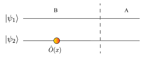
We expect the following development of $d^{2}(t)$ for the one dimensional system shown in Fig. 1. The local perturbation $\hat{O}(x,t=0)$ is outside of subsystem A, so at $t=0$, the distance $d^{2}(t=0)$ is strictly equal to zero. As time evolves, the operator $\hat{O}(x,-t)$ spreads out in the space and as it reaches the subsystem $A$, $d^{2}(t)$ becomes nonzero and increases with time. After sufficient long time, $\hat{O}(x,-t)$ has spread over the entire space and $d^{2}(t)$ will saturate to a constant.

Figure 1: The setup for computing $d^{2}(t)$.

III The spin chain models with local interaction

III.1 Floquet spin-$\frac{1}{2}$ chain

The dynamics of the Floquet (periodically driven) system is determined by the unitary time evolution operator over one period, namely the Floquet operator. Following Ref. Kim_2014, , we consider the following Floquet operator:

$$\hat{U}_{F}=\exp[-i\tau\hat{H}_{z}]\exp\left[-i\tau\hat{H}_{x}\right]~{},$$ (4)

where

$$\hat{H}_{x}=\sum_{j=1}^{L}g\hat{\sigma}_{j}^{x}$$

$$\hat{H}_{z}=\sum_{j=1}^{L-1}\hat{\sigma}_{j}^{z}\hat{\sigma}_{j+1}^{z}+\sum_{j=1}^{L}h\hat{\sigma}_{j}^{z}~{}.$$ (5)

This model is a one dimensional periodically driven system with period $T=2\tau$. In the numerical calculation, we choose open boundary condition with number of sites $L=24$. The system parameters are $(g,h)=(0.9045,0.8090)$. The parameter $\tau$ controls the period of the Floquet operator.

For both numerical and analytical convenience, we choose the initial state $|\psi_{1}\rangle$ as the Page state, which is defined as,

$$|\Psi(\{\alpha_{i}\})\rangle=\sum_{i}\alpha_{i}|C_{i}\rangle$$ (6)

where the coefficients $\alpha_{i}$ of the state in a fixed basis $\{|C_{i}\rangle\}_{i}$ are random complex numbers subject to the normalization constraint, with a probability distribution invariant under a unitary basis transformation. This state has (almost) maximal entanglement entropy and was first studied in detail by D. PagePage1993 . $|\psi_{2}\rangle$ is obtained by acting a local Hermitian operator $\hat{O}(x)=\hat{\sigma}^{x}(x)$ at location $x$ on $|\psi_{1}\rangle$. We study the Hilbert-Schmidt distance $\overline{d^{2}(t)}$ between $|\psi_{1}(t)\rangle$ and $|\psi_{2}(t)\rangle$ under the unitary time evolution, where the over-line denotes averaging over the ensemble of the initial Page states $|\psi_{1}\rangle$.

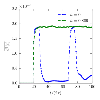
Since we are considering a Floquet model, the evolution time $t$ is an integer multiple of period, $t=nT$ with $n\in\mathbb{Z}_{+}$. There are in total three parameters we can tune: the half period of Floquet system $\tau$, the length $L_{A}$ of the subsystem A and the location of the local operator $x$. We first fix $L_{A}=6$, $x=1$ and change $\tau$. As shown in Fig. 2, when $t/T<18$, $\hat{O}(x,-t)$ does not propagate to region $A$ and we have $\overline{d^{2}}=0$. When $t\geq 18T$, $\overline{d^{2}(t)}$ starts to increase and eventually saturates to a small constant independent of $\tau$. How fast $\overline{d^{2}(t)}$ relaxes to the constant is $\tau$ dependent. When $\tau=0.8$, $\overline{d^{2}(t)}$ almost reaches the saturation value in one time step, suggesting rapid spreading of the local operator for this $\tau$ value.

Figure 2: (a) $\overline{d^{2}(t)}$ vs the time step $t/(2\tau)$ for various $\tau$ with fixed $L_{A}$ and $x$. (b) $\overline{d^{2}(t)}$ vs $t/(2\tau)$ for various $x$ with fixed $L_{A}$ and $\tau$. (c) Comparision between the saturation value of $\overline{d^{2}(t)}$ and $\overline{d^{2}(\hat{\rho}_{1},\hat{\rho}_{2})}$ between two independent Page states in Eq.(7).

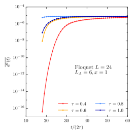
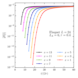
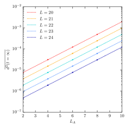
We present the dependence of $\overline{d^{2}(t)}$ on $x$ in Fig. 2. The time for $\overline{d^{2}(t)}$ starting to increase is linearly proportional to the distance between $\hat{\sigma}^{x}(x)$ and subsystem $A$. $\overline{d^{2}(t)}$ will eventually saturate to the same constant independent of $x$. Here we provide an interpretation for this saturation value. After long time evolution, the information of $\hat{O}(x,-t)$ is fully scrambled in the Hilbert space and we expect that $|\psi_{1}(t)\rangle$ and $|\psi_{2}(t)\rangle$ are close to two independent Page states. Since the reduced density matrix of Page state belongs to the fixed trace Wishart-Laguerre random matrix ensemble loggasrandommatrices ; mejia_difference_2017 , we can obtain an analytical result for $\overline{d^{2}(\hat{\rho}_{1},\hat{\rho}_{2})}$ of two independent Page states

$$\overline{d^{2}(\hat{\rho}_{1},\hat{\rho}_{2})}=\frac{2}{m}$$ (7)

where the subsystem $A$ and $B$ have dimensions $n=2^{L_{A}}$, $m=2^{L_{B}}$ with ratio $\alpha=n/m$ (The detail of this calculation can be found App. B). In Fig. 2, we present the saturation value of $\overline{d^{2}(t)}$ of the Floquet model and we find that they match well with $\overline{d^{2}(\hat{\rho}_{1},\hat{\rho}_{2})}$ of two independent Page states. In the thermodynamic limit $L\to\infty$ while keeping $L_{A}$ fixed, $\overline{d^{2}(\hat{\rho}_{1},\hat{\rho}_{2})}$ is exponentially small. We will explain why this constant is so small in the next section.

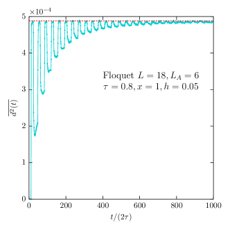
We further study the integrable system by tuning off the field in $z$ direction and compare it with the non-integrable system. The early time behaviors are rather similar for both $h=0.809$ (non-integrable) and $h=0$ ($z$ field off, integrable) as shown Fig. 3. However, in late times, $\overline{d^{2}(t)}$ saturates to constants in the non-integrable system while oscillates periodically in the integrable system. The oscillation behavior is caused by the ballistic quasi-particles created by the local operator $\hat{O}(x)$. Once the information has spread over the system, the quasi-particles will bounce back and forth periodically. As a result, the length of the system and the velocity of the quasi-particles determine the periodCardy2007 .

We also consider $h=0.05$ which weakly breaks the integrability and present the result in Fig. 3. Initially, the dynamics is similar to the case of $h=0$. As time evolves, the amplitude of the oscillation becomes smaller and vanishes after sufficiently long time evolution. We consider a relatively smaller system size $L=18$ since it takes very long time for $\overline{d^{2}(t)}$ to saturate. We find that the saturation value is again the same as that for two independent Page states. Therefore the integrability breaking term, albeit small, will eventually wash out the memory of the initial state and drive the system to the non-integrable behaviors.

Figure 3: (a) $\overline{d^{2}(t)}$ vs $t/(2\tau)$ for non-integrable system with $h=0.809$ and integrable system with $h=0$. (b) $\overline{d^{2}(t)}$ vs $t/(2\tau)$ for a system which weakly breaks integrability with $h=0.05$. The red dashed line on the top is $\overline{d^{2}}$ between two independent Page states.

III.2 Quantum Ising model with a longitudinal field

The Hamiltonian of the quantum Ising model with a longitudinal field is

$$\hat{H}_{\rm Ising}=-\sum_{i}\hat{\sigma}^{z}_{i}\hat{\sigma}^{z}_{i+1}-h_{x}\sum_{i}\hat{\sigma}^{x}_{i}-h_{z}\sum_{i}\hat{\sigma}^{z}_{i}~{}.$$ (8)

We take $(h_{x},h_{z})=(1.05,0.5)$Banuls2011 and compute $\overline{d^{2}(t)}$ for Page state ensemble under unitary time evolution governed by the Ising Hamiltonian $\hat{H}_{\rm Ising}$. The local perturbation is still $\hat{O}(x)=\hat{\sigma^{x}}(x)$.

We present the results in Fig. 4 for various $L_{A}$. As we move $\hat{O}(x)$ further away from subsystem $A$, it takes longer time, but eventually leads to a saturation of $\overline{d^{2}(t)}$ to a constant very close to values of two independent Page states. The growth of $\overline{d^{2}(t)}$ is always slower than an exponential function. This behavior is similar to that of the Floquet spin chain we studied in the previous section.

Figure 4: (a) $\overline{d^{2}(t)}$ vs time $t$ for Ising model defined in Eq.(8) on the semi-log scale, where the average is performed over 200 Page states. The dashed line is $\overline{d^{2}}$ between two independent Page states. (b) $\overline{d^{2}(t)}$ of the same model vs time $t$ for various $L$ on the semi-log scale, where the average is performed over 200 random product states. (c) $\overline{d^{2}(t)}$ vs time $t$ of two RPS states with energy close to zero under the same unitary time evolution.

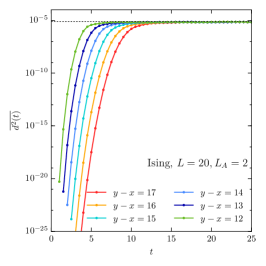
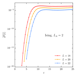
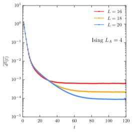
We also explore the initial state ensemble dependence of the saturation value. For the case of Ising model, we prepare another set of states that are random product states (RPS) with energy $E\in[-1,1]$. A RPS is a tensor product of state on each site whose spin directions are uniformly distributed on Bloch sphere. It thus has zero initial entanglement entropy (EE). We apply a perturbation on the RPS state and then compute the time dependent distance $\overline{d^{2}(t)}$. The results are presented in Fig. 4. The saturation values of $\overline{d^{2}(t)}$ for this set of initial states is different from the ones of two random states, but it still decays exponentially as we increase the system size.

The small saturation value of $\overline{d^{2}(t\to\infty)}$ can be understood in the following way. For a generic system, the initial wavefunction will eventually thermalize under its own dynamics at long times Srednicki1994 ; Deutsch1991 . In particular, it has been proven that in $1+1$d conformal field theory (satisfying generalized Gibbs ensemble Rigol2006 ; Rigol2007 ), the reduced density matrix of a small subsystem will relax to the thermal density matrix up to exponentially small corrections with the temperature determined by the initial energy density Cardy2015 . Therefore, if the two initial states have the same energy density, after sufficiently long time evolution, the reduced density matrix of both states will thermalize at the same effective temperature with $\overline{d^{2}(t)}$ approaching to a small constant. The Ising model considered here satisfies ETHBanuls2011 . The local perturbation applied to $|\psi_{2}\rangle$ will not change energy density and gives rise to an exponentially small saturation value of $\overline{d^{2}(t\to\infty)}$.

Furthermore, we study the saturation value of $d^{2}(t)$ when $|\psi_{1}\rangle$ and $|\psi_{2}\rangle$ are not connected by a local unitary transformation but have the same energy density. We choose $|\psi_{1}\rangle$ and $|\psi_{2}\rangle$ to be two different PRS states. At $t=0$, $\overline{d^{2}(t)}$ for subsystem $A$ is a $O(1)$ constant. After sufficiently long time evolution, $\overline{d^{2}(t)}$ relaxes to a small constant, which decreases exponentially as $L$ increases and is also consistent with ETH.

IV The spin chain models with power-law interaction

IV.1 Floquet spin-$\frac{1}{2}$ chain model

In this section, we consider Floquet model with power-law interaction

$$\hat{U}_{F}=\exp[-i\tau\hat{H}_{z}]\exp\left[-i\tau\hat{H}_{x}\right]~{},$$ (9)

where

$$\hat{H}_{x}=\sum_{j=1}^{L}g\hat{\sigma}_{j}^{x}$$

$$\hat{H}_{z}=\sum_{j>k}\frac{\hat{\sigma}_{j}^{z}\hat{\sigma}_{k}^{z}}{(j-k)^{\alpha}}+\sum_{j=1}^{L}h\hat{\sigma}_{j}^{z}~{}.$$ (10)

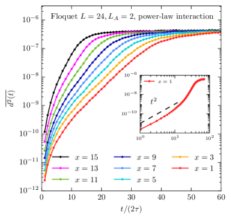
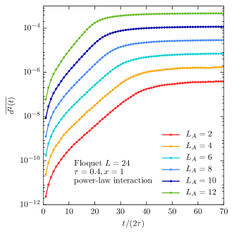
We fix parameter $(g,h,\tau)=(0.9045,0.8090,0.4)$ and compute $\overline{d^{2}(t)}$ averaged over the Page state ensemble. We take the power law exponent $\alpha=2.0$.

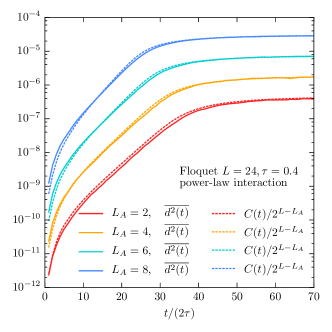
As shown in Fig. 5, when the distance between region $A$ and $\hat{\sigma}^{x}(x)$ is large, we can observe a clear intermediate fast growing regime. It has positive curvature on the log-log scale in the inset, indicating that it is faster than any power law growth. The fact that it is a straight line on the semi-log plot confirms the existence of an exponential growth regime.

This is different from the spin chain models with local interaction, where an exponentially growing regime is invisible in the parameter range we choose. The physical interpretation for this regime will be given in Sec. V.

Notice that at early time, $\overline{d^{2}(t)}$ scales as $t^{2}$ (inset of Fig. 5), which can be understood by taking short time expansion for $\hat{\sigma}^{x}(x,-t)$. Similar behavior is also found in Ref. Dora2017, and we will not discuss it here.

For fixed $L_{A}$, as we decrease the distance between $\hat{\sigma}^{x}(x)$ and subsystem $A$, this intermediate exponentially growing regime becomes smaller and vanishes eventually. Nevertheless, $\overline{d^{2}(t)}$ always saturates to the same constant, which is also the same as that of two independent Page states. We also present $\overline{d^{2}(t)}$ for various $L_{A}$ with fixed $x=1$ in Fig. 5. As we increase the subsystem length $L_{A}$, the distance between $x$ and the subsystem $A$ reduces, and therefore the exponentially growing regime becomes smaller. We observe that the growth rate is not very sensitive to the distance between $\hat{\sigma}^{x}(x)$ and region $A$.

Notice that when $L_{A}=2$, $\overline{d^{2}(t)}$ is averaged of 200 Page states due to large fluctuation in the data. When the subsystem has $L_{A}\geq 4$, the fluctuation is much smaller and the ensemble average is unnecessary. In the numerical calculation, we take average over 8 states.

Figure 5: (a) $\overline{d^{2}(t)}$ vs $t/(2\tau)$ for various $x$ with fixed $L_{A}$ on the semi-log scale for Floquet operator in Eq.(9). The average is over $200$ Page states. (b) $\overline{d^{2}(t)}$ vs $t/(2\tau)$ for various $L_{A}$ with fixed $x$ on the semi-log scale. We perform $200$ Pages states average for $L_{A}=2$ and $8$ Page states average for $L_{A}\geq 4$.

IV.2 Ising model with power-law interaction

We now consider a static Hamiltonian with a non-local power-law interaction,

$$\hat{H}=-\sum_{j>k}\frac{\hat{\sigma}^{z}_{j}\hat{\sigma}^{z}_{k}}{(j-k)^{\alpha}}-h_{x}\sum_{i}\hat{\sigma}^{x}_{i}-h_{z}\sum_{i}\hat{\sigma}^{z}_{i}~{}.$$ (11)

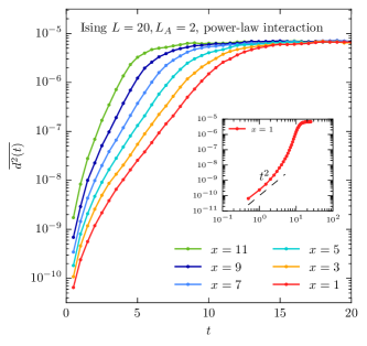
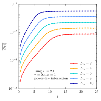
where we fix the parameter $(h_{x},h_{z})=(1.05,0.5)$ to be the same as in Eq.(8). We take the power law exponent $\alpha=2.1$, where we find the longest exponentially growing regime for $\overline{d^{2}(t)}$.

We still take $|\psi_{1}\rangle$ as a Page state and $|\psi_{2}\rangle=\hat{\sigma}^{x}(x)|\psi_{1}\rangle$. As we can observe in Fig. 6, the non-local power-law interaction leads to an exponentially growing regime in $\overline{d^{2}(t)}$, which becomes longer as we increase the distance between $\hat{\sigma}^{x}(x)$ and region $A$. The saturation value of $\overline{d^{2}(t)}$ is still the same as that for two independent Page states.

Figure 6: (a) $\overline{d^{2}(t)}$ vs $t$ for various $x$ with fixed $L_{A}$ on the semi-log scale for Ising model in Eq.(11). The average is over $200$ Page states. (b) $\overline{d^{2}(t)}$ vs $t$ for various $L_{A}$ with fixed $x$ on the semi-log scale. We perform $200$ Pages states average for $L_{A}=2$ and $8$ Page states average for $L_{A}\geq 4$.

V Connection between $d^{2}(t)$ and the square of commutator

In this section, we use the operator spreading picture to interpret the behaviors of $d^{2}(t)$ and relate it to the square of commutator. We will show that they are essentially the same quantity after a proper rescaling in the models we consider.

V.1 $d^{2}(t)$ in operator spreading picture

For simplicity, we will restrict our discussion to the spin-$\frac{1}{2}$ chain that is numerically studied in this paper, but a generalization to models with $q>2$ dimensional on-site Hilbert space is straightforward.

On each site of the spin-$\frac{1}{2}$ chain, we can define a local operator basis which consists of the identity operator $\hat{I}_{2}$ and the three Pauli matrices $\hat{\sigma}^{x}$, $\hat{\sigma}^{y}$, $\hat{\sigma}^{z}$. Using the tensor product of the local basis, we can build a complete operator basis $\{\hat{H}_{j}\}$ for the entire Hilbert space, in which each operator $\hat{H}_{j}$ is a string of $\hat{\sigma}^{x,y,z}$ and $\hat{I}_{2}$. This basis has a natural inner product $\mbox{Tr}(\hat{H}_{i}\hat{H}_{j})=\delta_{ij}|H|$, where $|H|$ is the size of the Hilbert space. We can choose $4^{L_{B}}$ operators $\{B_{j}\}$ from $\{H_{j}\}$ which consists of only identity operators in region $A$. They form an operator basis completely confined in region $B$. The average over these operators can be used to take a partial trace on any operator $\hat{O}$ in the full Hilbert space Hosur_2016 ,

$$\frac{1}{|B|}\sum_{i}\hat{B_{i}}\hat{O}\hat{B}_{i}=\mbox{Tr}_{B}(\hat{O})\otimes\hat{I}_{B}$$ (12)

where $|B|$ is the Hilbert space dimension of region $B$. A corollary of this identity is that for any operator $\hat{O}$

$$\operatorname{Tr}_{A}(\operatorname{Tr}_{B}\hat{O}\operatorname{Tr}_{B}\hat{O})=\operatorname{Tr}_{A}\operatorname{Tr}_{B}((\operatorname{Tr}_{B}\hat{O}\otimes I_{B})\hat{O})=\frac{1}{|B|}\sum_{i}\operatorname{Tr}(B_{i}\hat{O}B_{i}\hat{O})$$ (13)

This equation has been used to show the connection between the OTO correlator and operator entanglement entropy Hosur_2016 ; Fan_2016 ; harrow_random_2009 .

Figure 7: Diagrammatic proof of Eq.(13). The top channel corresponds to the region $A$ and the bottom channel corresponds to the region $B$. Dotted line indicates summation over $\hat{B}$ operators.

Using the above identity, we are going to rewrite $d^{2}(t)$ in terms of spreading of local operator in real space. For the pure state under unitary time evolution, the reduced density matrix for region A (after tracing out region B) takes the form,

$$\hat{\rho}(t)=\mbox{Tr}_{B}\left[\hat{U}(t)|\psi\rangle\langle\psi|\hat{U}^{{\dagger}}(t)\right]$$ (14)

The difference of the time dependent density matrices in region $A$ is $\hat{\rho}_{1}(t)-\hat{\rho}_{2}(t)=\hat{U}(t)\hat{V}\hat{U}^{\dagger}(t)$, where $\hat{V}=|\psi_{1}\rangle\langle\psi_{1}|-|\psi_{2}\rangle\langle\psi_{2}|$. Therefore the time dependent distance is

$$d^{2}(t)=\mbox{Tr}_{A}\left[\mbox{Tr}_{B}\hat{U}(t)\hat{V}\hat{U}^{{\dagger}}(t)\right]^{2}=\frac{1}{|B|}\sum_{i}\mbox{Tr}\left[\hat{B}_{i}(t)\hat{V}\hat{B}_{i}(t)\hat{V}\right]$$ (15)

where $\hat{B}_{i}(t)=\hat{U}^{{\dagger}}(t)\hat{B}_{i}\hat{U}$. The above equation is obtained by using the operator identity in Eq.(13) and is also diagrammatically interpreted in Fig. 7.

By plugging the explicit form of $\hat{V}$ into Eq.(15), we can expand $d^{2}(t)$ as

$$d^{2}(t)=\frac{1}{|B|}\sum_{i}\left[\langle\psi_{1}|\hat{B}_{i}(t)|\psi_{1}\rangle^{2}+\langle\psi_{2}|\hat{B}_{i}(t)|\psi_{2}\rangle^{2}-2\langle\psi_{1}|\hat{B}_{i}(t)|\psi_{2}\rangle\langle\psi_{2}|\hat{B}_{i}(t)|\psi_{1}\rangle\right]$$ (16)

Take $|\psi_{1}\rangle$ as a Page state, we can use its properties (Eq.(43) and Eq.(44) in App. A) and obtain the following expression,

$$\overline{d^{2}(t)} =\frac{2}{|B|}\sum_{i}\frac{\operatorname{Tr}^{2}(\hat{B}_{i})-\operatorname{Tr}^{2}(\hat{B}_{i}\hat{O}(x,-t))}{|H|(|H|+1)}$$ (17)

$$=\frac{2}{|B|}\frac{|H|}{|H|+1}\left\{1-\frac{1}{|H|^{2}}\sum_{i}\mbox{Tr}^{2}\left[\hat{B}_{i}\hat{O}(x,-t)\right]\right\}$$

This is one of the most important results in this paper. Notice that this averaged result is state independent and depends only on the spreading of $\hat{O}(x,-t)$ in the Hilbert space. Specifically, $\hat{O}(x,-t)$ can always be expanded in the operator basis as

$$\hat{O}(x,-t)=\sum_{j}\alpha_{j}(t)\hat{H}_{j}$$ (18)

For Hermitian operators on Hermitian basis $\{\hat{H}_{j}\}$, the components $\alpha_{j}(t)$ are real numbers and they satisfy the normalization constraint $\sum_{j}\alpha_{j}(t)^{2}=1$. The trace with the basis $\{\hat{B}_{i}\}$ evaluates the component of $\hat{O}(x,-t)$ that is completely confined in region $B$. Therefore $\overline{d^{2}(t)}$ is proportional to the weights of the operator basis that is not entirely in region $B$.

The spreading of operator $\hat{O}(x,-t)$ depends on the behavior of the coefficients $\alpha_{j}(t)$ and gives rise to an effective hydrodynamical description in one dimensional chaotic systems Nahum2017 ; Keyserlingk2017 ; Khemani2017 ; Rakovszky2017 . As time evolves, the string operators dominating the sum in Eq.(18) grow spatially and we can define the end point distribution to measure the spreading of $\hat{O}(x,-t)$,

$$f_{R}(s,t)\equiv\sum_{j}\alpha_{j}(t)^{2}\delta(\text{right most site}(\hat{H}_{j})=s)$$ (19)

which counts all the components of the basis that ends at site $s$ at time $t$. It is subjected to the normalization

$$\int_{0}^{L}f_{R}(s,t)ds=1$$ (20)

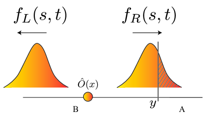
and can be interpreted as the (coarse grained) probability distribution of operators in $\hat{O}(-x,t)$ that ends at location $s$ at time $t$. One can similarly define the left end distribution $f_{L}(s,t)$.

Initially, the local operator $\hat{O}(x)$ only occupies one operator basis on one site. In early time, almost all operators contained in $\hat{O}(x,-t)$ are confined in region $B$, hence $\overline{d^{2}(t)}$ is small. Under the chaotic evolution, the end points distribution should move outwards on the left and right ends. Fig. 8 is the schematic of the shape of the distribution at late times. If the right end points of most operators are moving to the right, the distribution $f_{R}(s,t)$ should have a sharp wave front. Once the wave front crosses the cut at $y$, there will be an appreciable fraction of operators in $\hat{O}(x,-t)$ that has spread into region $A$, which contributes to the rapid growth of $d^{2}(t)$. In fact, the area of the wave front cut by the boundary of $A$ and $B$ is proportional to $\overline{d^{2}(t)}$,

$$\overline{d^{2}(t)}=\frac{2}{|B|}\frac{|H|}{(|H|+1)}\int_{y}^{L}f_{R}(s,t)ds\sim\frac{2}{|B|}\int_{y}^{L}f_{R}(s,t)ds$$ (21)

After sufficiently long time evolution, we expect that all the string operators in $\hat{O}(x,-t)$ have spanned the entire system. This means that $f_{R}(s,t)$ is localized at $s=L$ and $\overline{d^{2}(t)}$ saturates to

$$\overline{d^{2}(t)}\sim\frac{2}{|B|}$$ (22)

This is consistent with analytical result of the distance of two independent Page states (see App. B)

Figure 8: The schematics of the wave front $f_{L}(s,t)$ and $f_{R}(s,t)$ of $\hat{O}(x,-t)$.

V.2 $d^{2}(t)$ and square of commutator

We would like to compare $d^{2}(t)$ with another interesting quantity, the square of commutator

$$C(t)=-\frac{1}{|H|}\operatorname{Tr}[\hat{O}(x,-t),\hat{O}^{\prime}(y)]^{2}$$ (23)

where we take $\hat{O}^{\prime}(y)$ as a local Pauli operator sitting at position $y$ that does not evolve. We will just take it be $\hat{\sigma}^{x}$. In the operator basis we choose, only those do not commute with $\hat{O}^{\prime}(y)$ will contribute to $C(t)$, i.e.,

$$C(t)=-\sum_{j}\alpha_{j}^{2}(t)\frac{1}{|H|}\operatorname{Tr}[\hat{H}_{j},\hat{\sigma}^{x}(y)]^{2}=4\sum_{j}\alpha_{j}^{2}(t)\delta(\hat{H}_{j}\big{|}_{y}=\hat{\sigma}^{y,z})$$ (24)

Under the chaotic evolution, it is reasonable to assume that the probability of having $\hat{\sigma}^{x,y,z}$ and $\hat{I}$ are essentially the same . As a result, roughly half (in total weight) of the operators going across the position $y$ will contribute and hence

$$C(t)=\frac{1}{2}4\sum_{j}\alpha_{j}^{2}(t)\delta(\text{right most site}\geq y)=2\int_{y}^{L}dsf_{R}(s,t)$$ (25)

We therefore show that $\overline{d^{2}(t)}$ is essentially the rescaled version of $C(t)$ with the same distance $|y-x|$ in these chaotic systems

$$\overline{d^{2}(t)}=\frac{1}{|B|}C(t)$$ (26)

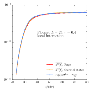
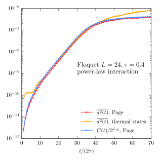
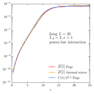
The numerical verification of the collapse is shown in Fig. 9 and Fig. 10. Notice that $\overline{C_{s}(t)}$ we compute is averaged over Page ensemble,

$$\overline{C_{s}(t)}=-\overline{\langle\psi|[\hat{O}(x,-t),\hat{O}^{\prime}(y)]^{2}|\psi\rangle}$$ (27)

which is equivalent to $C(t)$ defined in Eq.(23) (using the identity Eq.(43)). The collapse is an evidence that both $\overline{d^{2}(t)}$ and $C(t)$ measure the area of the wave front in the chaotic many-body systems.

Figure 9: (a) $\overline{d^{2}(t)}$ and $\overline{C_{s}(t)}$ vs $t/(2\tau)$ on the semi-log scale for Floquet operator in Eq.(4) with local interaction ($L_{A}=2$). (b) $\overline{d^{2}(t)}$ and $\overline{C_{s}(t)}$ vs $t/(2\tau)$ on the semi-log scale for Floquet operator in Eq.(9) with power-local interaction ($L_{A}=2$). The slope of the curve (for the exponentially growing regime) is $0.244$. (c) $\overline{d^{2}(t)}$ and $\overline{C_{s}(t)}$ vs $t$ on the semi-log scale for the static Hamiltonian in Eq.(8) with local interaction. (d) $\overline{d^{2}(t)}$ and $\overline{C_{s}(t)}$ vs $t$ on the semi-log scale for the static Hamiltonian in Eq.(11). The slope of the curve (for the exponentially growing regime) is $0.902$. In (a),(b) and (d), we take $\hat{O}(x,t=0)=\hat{\sigma}^{x}$ in $\overline{d^{2}(t)}$ and $\hat{O}(x,t=0)=\hat{O}^{\prime}(y)=\hat{\sigma}^{x}$ in $\overline{C_{s}(t)}$. In (c), for $\overline{C_{s}(t)}$, we fix $\hat{O}(x,t=0)=\hat{\sigma}^{z}$ and consider $\hat{O}^{\prime}(y)=\hat{\sigma}^{z}$ (red curve) and $\hat{O}^{\prime}(y)=\hat{\sigma}^{x}$ (yellow curve). The difference between these two curves at early time is because $\sigma^{z}$ has a larger overlap with energy density operator. The $\overline{d^{2}(t)}$ of $\hat{O}(x,t=0)=\hat{\sigma}^{z}$ (dashed black curve) lies in the middle between the red and blue curves.

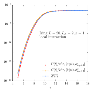
One interesting question is: how does $\overline{d^{2}(t)}$ or $C(t)$ grow with the time? Based on the arguments above, we can see that it depends on the shape of the operator wave front and the way it propagates, which is ultimately determined by the form of the interaction. For spin-$\frac{1}{2}$ chain with local interaction, we do not find an obvious exponentially growing regime in $\overline{d^{2}(t)}$ and $C(t)$. The absence of Lyapunov regime in spin-$1/2$ chain model is also discussed in Ref. Luitz2017, and is different from the classical chaotic spin chain model where we effectively have $S\to\infty$Wijn2013 . This is consistent with recent study in the random tensor network with local unitary time evolution, where $f_{R}(s,t)$ in the coarse grained picture is the probability distribution generated by a biased random walkNahum2017 ; Keyserlingk2017 . The distribution $f_{R}(s,t)$ is a moving Gaussian packet with the width of front broadened diffusively and there is no clear exponentially growing regime in $C(t)$.

However, non-local power-law interaction changes the story. As shown in Fig. 9 and 9, when the distance between $x$ and $y$ is large, we find a clear exponentially growing regime in both $\overline{d^{2}(t)}$ and $C(t)$. This is because the power-law interaction generates a wider wave packet in $f_{R}(s,t)$. We expect that when $|y-x|$ is large, the front has a near-exponential shape. To verify this point, we investigate $\overline{d^{2}(t)}$ and $C(t)$ for different distances $|y-x|$ at the same time $t$. As shown in Fig. 10, the area of the wave front in regime $A$ decreases exponentially as we increase the distance $|y-x|$. The slope seems to be invariant as we increase time $t$.

Figure 10: (a) $\overline{d^{2}(t)}$ and $\overline{C_{s}(t)}$ vs $t/(2\tau)$ on the semi-log scale for Floquet operator in Eq.(9) for various $y$ and fixed $x=1$ on the semi-log scale. (b) $2^{L_{B}-1}\overline{d^{2}(t)}$ (rescaled $d^{2}$) and $\overline{C_{s}(t)}/2$ vs the distance $|y-x|$ for various time $t$. Both quantities are measuring the area of the wave front in region $A$.

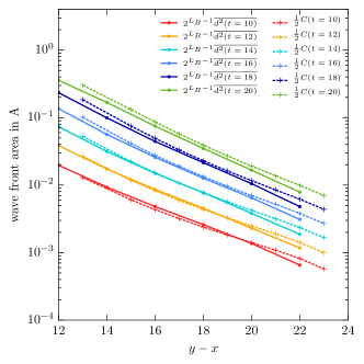
The near-exponential shape of the wave front is responsible for the exponentially growing regime in $\overline{d^{2}(t)}$ or $C(t)$, with the growth rate as the so-called quantum Lyapunov exponent, which is also found in some quantum many-body models in the large $N$ limitShenker2013a ; Shenker2013b ; Shenker2014 ; Maldacena2016 ; Kitaev2014 ; Kitaev2015 ; Sachdev1993 but is absent in the spin-$\frac{1}{2}$ chain with local interaction where $N=2$. It seems that the long-range power-law interaction effectively increases $N$ and gives rise to this Lyapunov regime. In the future, it would be interesting to have a better understanding on this Lyapunov regime and explore the dependence of Lyapunov exponent on the distance $|y-x|$ in some random non-local unitary tensor networks.

In most of the results, we use the Page states to compute $\overline{d^{2}(t)}$ for both simple numerical implementation and analytical control. They are however difficult to be generated in experiments. To resolve this issue, we also consider $\overline{d^{2}(t)}$ averaged over thermal states, which in comparison are more physical and much easier to be realized in the experiments. We prepare the thermal states by evolving the RPS states under unitary time evolution. After sufficiently long time evolution, these states will thermalize and can be used as the initial state for $\overline{d^{2}(t)}$. These thermal states share similar properties with the Page states but are subjected to some conservation laws determined by the Hamiltonian. In Fig. 9, we see that the thermal state average matches well with $\overline{d^{2}(t)}$ of the Page states for a large regime of time with both the Floquet evolution and time independent Hamiltonian. Notably, in spin model with non-local interactions, the thermal state average $\overline{d^{2}(t)}$ also grows exponentially with time, showing the same behavior as Page ensemble.

VI Conclusion

In conclusion, we study Hilbert-Schmidt distance $d^{2}(t)$ between reduced density matrices of two many-body wave functions initially differed by a local perturbation. Under unitary time evolution governed by a chaotic Hamiltonian, $\overline{d^{2}(t)}$ grows with time and eventually saturates to a small constant. In contrast to the exponential divergence of nearby trajectories in classical chaos, the growth of $\overline{d^{2}(t)}$ depends on the form of the interactions in the non-integrable models. We find that for spin-$\frac{1}{2}$ chain model with non-local power-law interaction, $\overline{d^{2}(t)}$ has a clear exponential growing regime if the local perturbation is far away from the subsystem. While for spin-$\frac{1}{2}$ chain with local interaction, $\overline{d^{2}(t)}$ always grows slower than the exponential function.

Moreover, we show that after sufficiently long time evolution, $\overline{d^{2}(t)}$ will approach a small constant, indicating the thermalization of a small subsystem in a many-body quantum state.

We further use operator scrambling picture to show that $\overline{d^{2}(t)}$ is the rescaled area of the wave front of the evolved local perturbation operator. The same interpretation also applies to the square of the commutator $C(t)$ under chaotic evolution. Hence the growth scaling of $\overline{d^{2}(t)}$ is determined by the shape of the wave front, which is ultimately determined by the form of interactions. From the collapse of the numerical data of $C(t)$ and $\overline{d^{2}(t)}$, we conclude that the exponent in the exponential growing region of $\overline{d^{2}(t)}$ is the quantum Lyapunov exponent which was previously observed in some large $N$ models.

Appendix A Average over Page ensemble

In this section, we compute the expectation values $\overline{\langle\psi|\hat{O}|\psi\rangle}$ and $\overline{\langle\psi|\hat{O}_{1}|\psi\rangle\langle\psi|\hat{O}_{2}|\psi\rangle}$ over the Page ensemble. For the ease of notation, we will reserve $n$ to denote the complex dimension of the Hilbert space. When comparing the result with main text, $n$ should be identified with $|H|$.

A.1 Probability Measure

The random pure state (Page state) has a probability measure that is uniform in the Hilbert space. Such a uniform measure has ${\rm U}(n)$ invariance, meaning that the average is invariant under the ${\rm U}(n)$ action, e.g.

$$\overline{\langle\psi|\hat{O}|\psi\rangle}=\overline{\langle\psi|U^{\dagger}\hat{O}U|\psi\rangle},\quad\forall U\in{\rm U}(n)$$ (28)

Such invariance can be constructed by choosing complex Gaussian random variables as the coefficients in an orthonormal basis. For vector $\bm{\mathbf{c}}\in\mathbb{C}^{n}$, whose component $c_{i}$ are sampled from standard complex normal distribution, we have the required invariance,

$$\mathbb{E}(U\bm{\mathbf{c}}) =U\mathbb{E}(\bm{\mathbf{c}})=\bm{\mathbf{0}}=\mathbb{E}(\bm{\mathbf{c}})$$ (29)

$$\mathbb{E}(U(\bm{\mathbf{c}}-\mu)U(\bm{\mathbf{c}}-\mu)^{\dagger}U^{\dagger}) =U\mathbb{E}(\bm{\mathbf{c}}\bm{\mathbf{c}}^{\dagger})U^{\dagger}=\mathbb{I}=\mathbb{E}(\bm{\mathbf{c}}\bm{\mathbf{c}}^{\dagger})$$

This is how we generate the Page state in the numerical calculation.

Writing $c_{j}=x_{2j-1}+ix_{2j}$, the $N=2n$-dimensional real vector $\bm{\mathbf{x}}$ has independent real Gaussian random variable as its component. With the normalization constraint, the probability measure is

$$d\mu\propto \exp(-\frac{1}{2}|\bm{\mathbf{x}}|^{2})\delta(1-|\bm{\mathbf{x}}|^{2})\prod_{i}dx_{i}\propto\delta(1-|\bm{\mathbf{x}}|^{2})\prod_{i}dx_{i}$$ (30)

which is the uniform measure on the $2n-1$ dimensional sphere. The expectation value of the state $\overline{\langle\psi|\hat{O}|\psi\rangle}$ is a function (polynomial) $f(\bm{\mathbf{x}})$ of real and imaginary parts of the elements. Averaging over the random states is given by the integral

$$\overline{\langle\psi|\hat{O}|\psi\rangle}=\int_{S_{N-1}}d\mu\,f(\bm{\mathbf{x}})$$ (31)

A.2 Moments of the probability measure

The $\overline{\langle\psi|\hat{O}|\psi\rangle}$ and $\overline{\langle\psi|\hat{O}_{1}|\psi\rangle\langle\psi|\hat{O}_{2}|\psi\rangle}$ can be converted to the average over the coefficients of the Page state, e.g.

$$\overline{\langle\psi|\hat{O}|\psi\rangle} =O_{ij}\overline{c_{i}^{*}c_{j}}=O_{ij}\overline{(x_{2i-1}-ix_{2i})(x_{2j-1}+ix_{2j})}$$ (32)

$$\overline{\langle\psi|\hat{O}_{1}\psi\rangle\langle\psi|\hat{O}_{2}|\psi\rangle} =O^{1}_{ij}O^{2}_{kl}\overline{(x_{2i-1}-ix_{2i})(x_{2j-1}+ix_{2j})(x_{2k-1}-ix_{2k})(x_{2l-1}+ix_{2l})}$$

hence we need up to 4th order moments of $x_{i}$.

By the reflection symmetry, there are only 3 types of moments that need to be computed,

$$A_{1}=\int d\mu\,x_{i}^{2},\quad\int d\mu\,x_{i}^{2}x_{j}^{2}=\left\{\begin{aligned} A_{2}&\quad i=j\\ B_{2}&\quad i\neq j\\ \end{aligned}\right.$$ (33)

The 2nd moment

$$A_{1}=\int d\mu\,x_{i}^{2}=\frac{1}{N}\int d\mu|\bm{\mathbf{x}}|^{2}=\frac{1}{N}$$ (34)

is be obtained by ${\rm O}(N)$ symmetry, which also relates $A_{2}$ and $B_{2}$,

$$1=\int d\mu\,|\bm{\mathbf{x}}|^{2}\times|\bm{\mathbf{x}}|^{2}=NA_{2}+N(N-1)B_{2}$$ (35)

So we only need $A_{2}$ or $B_{2}$.

We first compute the normalization constant, which is proportional to the area of sphere

$$\int_{\mathbb{R}^{N}}\delta(1-|\bm{\mathbf{x}}|^{2})\prod_{i}dx_{i} =\int_{0}^{\infty}r^{N-1}dr\delta(1-r^{2}){\rm S}_{N-1}$$ (36)

$$=\frac{1}{2}{\rm S}_{N-1}\int_{0}^{\infty}\delta(1-r^{2})r^{N-2}dr^{2}=\frac{1}{2}{\rm S}_{N-1}$$

With this we can compute $A_{2}$ with the remaining ${\rm O}(N-1)$ symmetry,

$$A_{2} =\frac{2}{{\rm S}_{N-1}}\int x_{1}^{4}\delta(1-|\bm{\mathbf{x}}|^{2})\prod_{i}dx_{i}=\frac{{\rm S}_{N-2}}{{\rm S}_{N-1}}\int_{0}^{\infty}dr^{2}\int_{0}^{\infty}dx^{2}_{1}\,\delta(1-x_{1}^{2}-r^{2})r^{N-3}x^{3}_{1}$$ (37)

$$=\frac{{\rm S}_{N-2}}{{\rm S}_{N-1}}\int_{0}^{1}dx\,x^{\frac{3}{2}}(1-x)^{\frac{N-3}{2}}=\frac{{\rm S}_{N-2}}{{\rm S}_{N-1}}\frac{3\sqrt{\pi}}{4}\frac{\Gamma(\frac{N-1}{2})}{\Gamma(\frac{N}{2}+2)}$$

$$=\frac{3}{4}\frac{\Gamma(\frac{N}{2})}{\Gamma(\frac{N}{2}+2)}=\frac{3}{N(N+2)}\implies B_{2}=\frac{1}{N(N+2)}$$

In fact, the general pure $2k$ moments can be computed similarly

$$A_{2k} =\frac{2}{{\rm S}_{N-1}}\int x_{1}^{2k}\delta(1-|\bm{\mathbf{x}}|^{2})\prod_{i}dx_{i}=\frac{(2k-1)!!}{(N+2k-2)(N+2k-4)\cdots N}$$ (38)

Now we apply these results to the quantity we need to compute in Eq.(32), where $N=2n$. We have the 2nd moments

$$\overline{c^{*}_{i}c_{j}}=\overline{(x_{2i-1}-ix_{2i})(x_{2j-1}+ix_{2j})}=\delta_{ij}\frac{2}{N}=\frac{1}{n}\delta_{ij}$$ (39)

The general 4th moments reduces to three types of contractions

$$\overline{c_{i}^{*}c_{j}c_{k}^{*}c_{l}} =(\delta_{ij}\delta_{kl}+\delta_{il}\delta_{jk})\overline{c_{i}^{*}c_{i}c_{k}^{*}c_{k}}(1-\delta_{ik})+\delta_{ik}\delta_{jl}\overline{c_{i}^{*}c_{i}^{*}c_{j}c_{j}}(1-\delta_{ij})+\delta_{ij}\delta_{jk}\delta_{kl}\overline{c_{i}^{*}c_{i}c_{i}^{*}c_{i}}$$ (40)

where each of them can be represented by $A_{2}$ and $B_{2}$

$$\overline{c_{i}^{*}c_{i}c_{k}^{*}c_{k}}(1-\delta_{ik}) =(1-\delta_{ik})\overline{(x_{2i-1}^{2}+x_{2i}^{2})(x_{2k-1}^{2}+x_{2k}^{2})}$$ (41)

$$=(1-\delta_{ik})4B_{2}=(1-\delta_{ik})\frac{1}{n(n+1)}$$

$$\overline{c_{i}^{*}c^{*}_{i}c_{j}c_{j}}(1-\delta_{ij}) =(1-\delta_{ij})\overline{(x_{2i-1}^{2}-x_{2i}^{2}-2ix_{2i-1}x_{2i})(x_{2j-1}^{2}-x_{jk}^{2}+2ix_{2j-1}x_{2j})}$$

$$=(1-\delta_{ij})(2B_{2}-2B_{2})=0$$

$$\overline{c_{i}^{*}c_{i}c_{i}^{*}c_{i}} =\overline{(x_{2i-1}^{2}+x_{2i}^{2})^{2}}=\frac{2}{n(n+1)}$$

Therefore we have ”Wick theorem” for the moments of $c_{i}$

$$\overline{c_{i}^{*}c_{j}c_{k}^{*}c_{l}} =(\delta_{ij}\delta_{kl}+\delta_{il}\delta_{jk})\frac{1}{n(n+1)}(1-\delta_{ik})+\frac{2}{n(n+1)}\delta_{ik}\delta_{jl}\delta_{ij}$$ (42)

$$=(\delta_{ij}\delta_{kl}+\delta_{il}\delta_{jk})\frac{1}{n(n+1)}$$

A.3 Average of expectation values

We apply the results of the previous sections to the average of expectation values. For operator $\hat{O}$, we have

$$\overline{\langle\psi|\hat{O}|\psi\rangle} =O^{ij}\overline{c_{i}^{*}c_{j}}=\frac{1}{n}\delta_{ij}O^{ij}=\frac{1}{n}\operatorname{Tr}(\hat{O})$$ (43)

For two operators $\hat{O}_{1}$ and $\hat{O}_{2}$, we have

$$\overline{\langle\psi|\hat{O}_{1}|\psi\rangle\langle\psi|\hat{O}_{2}|\psi\rangle} =O_{1}^{ij}O_{2}^{kl}\overline{c_{i}^{*}c_{j}c_{k}^{*}c_{l}}=\frac{1}{n(n+1)}O_{1}^{ij}O_{2}^{kl}(\delta_{ij}\delta_{kl}+\delta_{il}\delta_{jk})$$ (44)

$$=\frac{1}{n(n+1)}[\operatorname{Tr}(\hat{O}_{1}\hat{O}_{2})+\operatorname{Tr}(\hat{O}_{1})\operatorname{Tr}(\hat{O}_{2})]$$

where $n$ is the Hilbert space dimension $|H|$ in the main text.

Appendix B Averaged distance of two independent Page states

As discussed in App. A, the random pure state (Page state) can be constructed by assigning complex Gaussian random variables as the coefficients in any orthonormal basis.

We divide the Hilbert space into subsystem $A$ with dimension $n$ and $B$ with dimension $m\geq n$. In the same orthonormal basis, we can obtain the decomposition coefficients $\psi_{ij}$ of the wavefunction on the subsystem basis. Call this $n\times m$ matrix $Y$, the reduced density matrix is $\hat{\rho}_{A}=YY^{\dagger}$. The reduced density matrix consists of products of Gaussian random variables, and thus is a Wishart matrix with unit trace constraint.

The element of $Y$ matrix satisfies a Gaussian probability distributionnadal_statistical_2011

$$P(\{Y_{ij}\})\sim\exp\left[\frac{\beta}{2}\operatorname{Tr}YY^{{\dagger}}\right]$$ (45)

where the Dyson index $\beta=2$ in this case. Therefore the eigenvalue of $YY^{{\dagger}}$ scales as $n$, and the (rescaled) spectral density is defined as

$$\varrho(x,\rho)=\frac{1}{n}\sum_{i}\delta(x-\frac{\lambda_{i}}{n}).$$ (46)

In the large $n$ limit (keeping the ratio $\alpha=\frac{n}{m}$ fixed), the spectral density reduces to the Marchenko-Pastur distribution with parameters

$$\varrho_{\,\!{}_{\rm W}}(x)=\frac{1}{2\pi x}\sqrt{(\frac{\alpha_{+}}{\alpha}-x)(x-\frac{\alpha_{-}}{\alpha})}$$ (47)

where $\alpha_{\pm}=(1\pm\sqrt{\alpha})^{2}$.

Wishart matrix with the trace constraint is called fixed trace Wishart-Laguerre ensemble. Due to the constraint, the eigenvalues scales as $\frac{1}{n}$, so we shall instead usenadal_statistical_2011 ; mejia_difference_2017

$$\varrho(x,\rho)=\frac{1}{n}\sum_{i}\delta(x-n\lambda_{i})$$ (48)

The corresponding asymptotic distribution is

$$\varrho_{\,\!{}_{\rm W,tr}}(x)=\frac{1}{2\pi\alpha x}\sqrt{(\alpha_{+}-x)(x-\alpha_{-})}$$ (49)

it is different from the one without the trace constraint.

The distance we want to compute is the second moments of the eigenvalues of $\hat{\rho}_{1}-\hat{\rho}_{2}$

$$d^{2}(t)=\operatorname{Tr}(\hat{\rho}_{1}-\hat{\rho}_{2})^{2}=\sum_{i}\lambda_{i}^{2}$$ (50)

which is the distribution of the difference of two independent variables sampled from the Marchenko-Pastur distribution. Because of the constraint $\sum_{i}\lambda_{i}=0$, the eigenvalues also scale as $\frac{1}{n}$,

$$\varrho(x,\hat{\rho}_{1}-\hat{\rho}_{2})=\frac{1}{n}\sum_{i}\delta(x-n\lambda_{i})$$ (51)

Taking a function $f(x)$, the average of the sum $\sum_{i}f(\lambda_{i})$ can be carried over the spectral density function

$$\frac{1}{n}\sum_{i=1}^{n}f(\lambda_{i}) =\int\,f(\lambda)\frac{1}{n}\sum_{i=1}^{n}\delta(\lambda-\lambda_{i})P(\{\lambda_{i}\})\,d\lambda$$ (52)

$$=\int\,f(\lambda)\frac{1}{n}\sum_{i=1}^{n}\delta(n\lambda-n\lambda_{i})P(\{\lambda_{i}\})\,dn\lambda$$

$$=\int f(\frac{x}{n})\varrho(x,\hat{\rho}_{2}-\hat{\rho}_{1})\,dx$$

Ref. mejia_difference_2017, computes the asymptotic eigenvalue distribution and its absolute moments

$$m_{z}=\int|x|^{z}\varrho(x)\,dx=\frac{\Gamma(z+1)(2\alpha)^{\frac{z}{2}}}{\Gamma(\frac{z}{2}+1)\Gamma(\frac{z}{2}+2)}{}_{2}F_{1}(1-\frac{z}{2},-\frac{z}{2};\frac{z}{2}+2;\frac{\alpha}{2})$$ (53)

where ${}_{2}F_{1}$ is the hypergeometric function. Hence

$$d^{2} =n\int\frac{1}{n^{2}}x^{2}\varrho(x)\,dx=\frac{1}{n}m_{2}=\frac{1}{n}(2\alpha){}_{2}F_{1}(0,-1;3;\frac{\alpha}{2})$$ (54)

$$=\frac{2\alpha}{n}=\frac{2}{m}$$

References

- [1] C. Schmidt O. Bohigas, M. J. Giannoni. Characterization of chaotic quantum spectra and universality of level fluctuation laws. Phys. Rev. Lett., 52:1, 1984.
- [2] Martin C Gutzwiller. Chaos in classical and quantum mechanics, volume 1. Springer Science & Business Media, 2013.
- [3] E. Leviatan, F. Pollmann, J. H. Bardarson, D. A. Huse, and E. Altman. Quantum thermalization dynamics with Matrix-Product States. arXiv preprint arXiv:1702.08894, 2017.
- [4] A. I. Larkin and Yu. N. Ovchinnikov. Quasiclassical Method in the Theory of Superconductivity. Soviet Journal of Experimental and Theoretical Physics, 28:1200, June 1969.
- [5] Matthew B. Hastings and Tohru Koma. Spectral gap and exponential decay of correlations. Communications in Mathematical Physics, 265(3):781–804, Aug 2006.
- [6] Zhe-Xuan Gong, Michael Foss-Feig, Spyridon Michalakis, and Alexey V. Gorshkov. Persistence of locality in systems with power-law interactions. Phys. Rev. Lett., 113:030602, Jul 2014.
- [7] Don N. Page. Average entropy of a subsystem. Phys. Rev. Lett., 71:1291–1294, Aug 1993.
- [8] C. W. von Keyserlingk, Tibor Rakovszky, Frank Pollmann, and S. L. Sondhi. Operator hydrodynamics, otocs, and entanglement growth in systems without conservation laws. Phys. Rev. X, 8:021013, Apr 2018.
- [9] Adam Nahum, Sagar Vijay, and Jeongwan Haah. Operator spreading in random unitary circuits. Phys. Rev. X, 8:021014, Apr 2018.
- [10] Stephen H. Shenker and Douglas Stanford. Black holes and the butterfly effect. Journal of High Energy Physics, 2014(3):1–25, 2014.
- [11] Stephen H. Shenker and Douglas Stanford. Multiple shocks. Journal of High Energy Physics, 2014(12):1–20, 2014.
- [12] Stephen H. Shenker and Douglas Stanford. Stringy effects in scrambling. Journal of High Energy Physics, 2015(5):1–34, 2015.
- [13] Juan Maldacena and Douglas Stanford. Remarks on the Sachdev-Ye-Kitaev model. Phys. Rev. D, 94:106002, Nov 2016.
- [14] A. Kitaev, 2014. Talks given at the Fundamental Physics Prize Symposium, Nov. 10, 2014, and at KITP, Feb. 12, 2015.
- [15] A. Kitaev, 2015. Talks at KITP, April 7, 2015 and May 27, 2015.
- [16] Subir Sachdev and Jinwu Ye. Gapless spin-fluid ground state in a random quantum heisenberg magnet. Phys. Rev. Lett., 70:3339–3342, May 1993.
- [17] Mark Srednicki. Chaos and quantum thermalization. Phys. Rev. E, 50:888–901, Aug 1994.
- [18] J. M. Deutsch. Quantum statistical mechanics in a closed system. Phys. Rev. A, 43:2046–2049, Feb 1991.
- [19] Hyungwon Kim, Tatsuhiko N. Ikeda, and David A. Huse. Testing whether all eigenstates obey the eigenstate thermalization hypothesis. Phys. Rev. E, 90:052105, Nov 2014.
- [20] P.J. Forrester. Log-Gases and Random Matrices (LMS-34). Princeton University Press, 2010.
- [21] José Mejía, Camilo Zapata, and Alonso Botero. The difference between two random mixed quantum states: exact and asymptotic spectral analysis. Journal of Physics A: Mathematical and Theoretical, 50(2):025301, January 2017.
- [22] Pasquale Calabrese and John Cardy. Quantum quenches in extended systems. Journal of Statistical Mechanics: Theory and Experiment, 2007(06):P06008, 2007.
- [23] M. C. Bañuls, J. I. Cirac, and M. B. Hastings. Strong and weak thermalization of infinite nonintegrable quantum systems. Phys. Rev. Lett., 106:050405, Feb 2011.
- [24] Marcos Rigol, Alejandro Muramatsu, and Maxim Olshanii. Hard-core bosons on optical superlattices: Dynamics and relaxation in the superfluid and insulating regimes. Phys. Rev. A, 74:053616, Nov 2006.
- [25] Marcos Rigol, Vanja Dunjko, Vladimir Yurovsky, and Maxim Olshanii. Relaxation in a completely integrable many-body quantum system: An ab initio study of the dynamics of the highly excited states of 1d lattice hard-core bosons. Phys. Rev. Lett., 98:050405, Feb 2007.
- [26] John Cardy. Quantum quenches to a critical point in one dimension: some further results. Journal of Statistical Mechanics: Theory and Experiment, 2016(2):023103, 2016.
- [27] Balázs Dóra and Roderich Moessner. Out-of-time-ordered density correlators in luttinger liquids. Phys. Rev. Lett., 119:026802, Jul 2017.
- [28] P. Hosur, X.-L. Qi, D. A. Roberts, and B. Yoshida. Chaos in quantum channels. Journal of High Energy Physics, 2:4, February 2016.
- [29] Ruihua Fan, Pengfei Zhang, Huitao Shen, and Hui Zhai. Out-of-time-order correlation for many-body localization. Science Bulletin, 62(10):707 – 711, 2017.
- [30] Aram W. Harrow and Richard A. Low. Random Quantum Circuits are Approximate 2-designs. Communications in Mathematical Physics, 291(1), October 2009.
- [31] Vedika Khemani, Ashvin Vishwanath, and David A Huse. Operator spreading and the emergence of dissipation in unitary dynamics with conservation laws. arXiv preprint arXiv:1710.09835, 2017.
- [32] Tibor Rakovszky, Frank Pollmann, and CW von Keyserlingk. Diffusive hydrodynamics of out-of-time-ordered correlators with charge conservation. arXiv preprint arXiv:1710.09827, 2017.
- [33] This assumption may not be valid in the presence of conservation law (See Fig. 9). Moreover, it may also break down in the chaotic system which weakly breaks integrability. All these problems deserve to be further explored in the future.
- [34] David J. Luitz and Yevgeny Bar Lev. Information propagation in isolated quantum systems. Phys. Rev. B, 96:020406, Jul 2017.
- [35] A S de Wijn, B Hess, and B V Fine. Lyapunov instabilities in lattices of interacting classical spins at infinite temperature. Journal of Physics A: Mathematical and Theoretical, 46(25):254012, 2013.
- [36] Celine Nadal, Satya N. Majumdar, and Massimo Vergassola. Statistical Distribution of Quantum Entanglement for a Random Bipartite State. Journal of Statistical Physics, 142(2):403–438, January 2011.