A Spectral Approach for the Design of Experiments: Design, Analysis and Algorithms

Abstract

This paper proposes a new approach to construct high quality space-filling sample designs. First, we propose a novel technique to quantify the space-filling property and optimally trade-off uniformity and randomness in sample designs in arbitrary dimensions. Second, we connect the proposed metric (defined in the spatial domain) to the objective measure of the design performance (defined in the spectral domain). This connection serves as an analytic framework for evaluating the qualitative properties of space-filling designs in general. Using the theoretical insights provided by this spatial-spectral analysis, we derive the notion of optimal space-filling designs, which we refer to as space-filling spectral designs. Third, we propose an efficient estimator to evaluate the space-filling properties of sample designs in arbitrary dimensions and use it to develop an optimization framework to generate high quality space-filling designs. Finally, we carry out a detailed performance comparison on two different applications in $2$ to $6$ dimensions: a) image reconstruction and b) surrogate modeling on several benchmark optimization functions and an inertial confinement fusion (ICF) simulation code. We demonstrate that the propose spectral designs significantly outperform existing approaches especially in high dimensions.

Keywords: design of experiments, space-filling, poisson-disk sampling, surrogate modeling, regression

1 Introduction

Exploratory analysis and inference in high dimensional parameter spaces is a ubiquitous problem in science and engineering. As a result, a wide-variety of machine learning tools and optimization techniques have been proposed to address this challenge. In its most generic formulation, one is interested in analyzing a high-dimensional function $f:\mathcal{D}\rightarrow\mathbb{R}$ defined on the $d$-dimensional domain $\mathcal{D}$. A typical approach for such an analysis is to first create an initial sampling $\mathcal{X}=\{\mathbf{x_{i}}\in\mathcal{D}\}_{i=1}^{N}$ of $\mathcal{D}$, evaluate $f$ at all $\mathbf{x_{i}}$, and perform subsequent analysis and learning using only the resulting tuples $\{(\mathbf{x_{i}},f(\mathbf{x_{i}}))\}_{i=1}^{N}$. Despite the widespread use of this approach, a critical question that still persists is: how should one obtain a high quality initial sampling $\mathcal{X}$ for which the data $f(\mathcal{X})$ is collected? This challenge is typically refered to as Design of Experiments (DoE) and solutions have been proposed as early as  (Fisher, 1935) to optimize agricultural experiments. Subsequently, DoE has received significant attention from researchers in different fields (Garud et al., 2017) as it is an important building block for a wide variety of applications, such as surrogate modeling, image reconstruction, reinforcement learning, or data analysis. In several scenarios, it has been shown that success crucially depends on the quality of the initial sampling $\mathcal{X}$. Currently, a plethora of sampling solutions exist in the literature with a wide-range of assumptions and statistical guarantees; see (Garud et al., 2017; Owen, 2009) for a detailed review of related methods. Conceptually, most approaches aim to cover the sampling domain as uniformly as possible, in order to generate the so called space-filling experimental designs. However, it is well know that uniformity alone does not necessarily lead to high performance. For example, optimal sphere packings lead to highly uniform designs, yet are well known to cause strong aliasing artifacts most easily perceived in many computer graphics applications. Instead, a common assumption is that a good design should balance uniformity and randomness. Unfortunately, an exact definition for what should be considered a good space-filling design remains elusive.

Most common approaches use various scalar metrics to encapsulate different notions of ideal sampling properties. One popular metric is the discrepancy of an experimental design, defined as an appropriate $\ell_{p}$ norm of the ratio of points within all (hyper-rectangular) sub-volumes of $\mathcal{D}$ and the corresponding volume ratio. In other words, discrepancy quantifies the non-uniformity of a sample design. The most prominent examples of so called discrepancy sequences are Quasi-Monte Carlo (QMC) methods and their variants (Caflisch, 1998). In their classical form, discrepancy sequences are deterministic though extensions to incorporate randomess have been proposed, for example, using digital scrambling (Owen, 1995). Nevertheless, by optimizing for discrepancy these techniques focus almost exclusively on uniformity, and consequently even optimized QMC patterns can be quite structured and create aliasing artifacts. Furthermore, even the fastest known strategies for evaluating popular discrepancy measures require $O(N^{2}d)$ operations making evaluation, let alone optimization, for discrepancy difficult even for moderate dimensions. Finally, for most discrepancy measures, the optimal achievable values are not known. This makes it difficult to determine whether a poorly performing sample design is due to the insufficiency of the chosen discrepancy measure or due to ineffective optimization.

Another class of metrics to describe sample designs are based on geometric distances. These can be used directly by, for example, optimizing the maximin or minimax distance of a sample design (Schlömer et al., 2011) or indirectly by enforcing empty disk conditions. The latter is the basis for the so-called Poisson disk samples (Lagae and Dutré, 2008), which aim to generate random points such that no two samples can be closer than a given minimal distance $r_{min}$, i.e. enforcing an empty disc of radius $r_{min}$ around each sample. Typically, Poisson-type samples are characterized by the relative radius, $\rho$, defined as the ratio of the minimum disk radius $r_{min}$ and the maximum possible disk radius $r_{max}$ for $N$ samples to cover the sampling domain. Similar to the discrepancy sequences, maximin and minimax designs exclusively consider uniformity, are difficult to optimize for especially in higher dimensions, and often lead to very regular patterns. Poisson disk samples use $\rho$ to trade off randomness (lower $\rho$ values) and uniformity (higher $\rho$ values). A popular recommendation in $2$-d is to aim for $0.65\leq\rho\leq 0.85$ as a good compromise. However, there does not exist any theoretical guidance for choosing $\rho$ and hence, optimal values for higher dimensions are not known. As discussed in more detail in Section 2, there also exist a wide variety of techniques that combine different metrics and heuristics. For example, Latin Hypercube sampling (LHS) aims to spread the sample points uniformly by stratification, and one can potentially optimize the resulting design using maximin or minimax techniques (Jin et al., 2005).

In general, scalar metrics to evaluate the quality of a sample design tend not to be very descriptive. Especially in high dimensions different designs with, for example, the same $\rho$ can exhibit widely different performance and for some discrepancy sequences the optimal designs converge to random samples in high dimensions (Morokoff and Caflisch, 1994; Wang and Sloan, 2008). Furthermore, one rarely knows the best achievable value of the metric, i.e. the lowest possible discrepancy, for a given problem which makes evaluating and comparing sampling designs difficult. Finally, most metrics are expensive to compute and not easily optimized. This makes it challenging in practice to create good designs in high dimensions and with large sample sizes.

To alleviate this problem, we propose a new technique to quantify the space-filling property, which enables us to systematically trade-off uniformity and randomness, consequently producing better quality sampling designs. More specifically, we use tools from statistical mechanics to connect the qualitative performance (in the spectral domain) of a sampling pattern with its spatial properties characterized by the pair correlation function (PCF). The PCF measures the distribution of point samples as a function of distances, thus, providing a holistic view of the space-filling property (See Figure 1). Furthermore, we establish the connection between the PCF and the power spectral density (PSD) via the $1-$D Hankel transform in arbitrary dimensions, thus providing a relation between the PCF and an objective measure of sampling quality to help subsequent design and analysis.

Using insights from the analysis of space-filling designs in the spectral domain, we provide design guidelines to systematically trade-off uniformity and randomness for a good sampling pattern. The analytical tractability of the PCF enables us to perform theoretical analysis in the spectral domain to derive the structure of optimal space-filling designs, referred to as space-filling spectral design in the rest of this paper. Next, we develop an edge corrected kernel density estimator based technique to measure the space-filling property via PCFs in arbitrary dimensions. In contrast to existing PCF estimation techniques, the proposed PCF estimator is both accurate and computationally efficient. Based on this estimator, we develop a systematic optimization framework and a novel algorithm to synthesize space-filling spectral designs. In particular, we propose to employ a weighted least-squares based gradient descent optimization, coupled with the proposed PCF estimator, to accurately match the optimal space-filling spectral design defined in terms of the PCF.

Note that, there is a strong connection between the proposed space-filling spectral designs and coverage based designs such as Poisson Disk Sampling (PDS) (Gamito and Maddock, 2009). However, the major difference lies in the metric/criterion these techniques use to estimate and optimize the space-filling designs. Furthermore, existing works on PDS focus primarily on algorithmic issues, such as worst-case running times and numerical issues associated with providing high-quality implementations. However, different PDS methods often demonstrate widely different performances which raises the questions of how to evaluate the qualitative properties of different PDS patterns and how to define an optimal PDS pattern? We argue that, coverage $(\rho)$ based metrics alone are insufficient for understanding the statistical aspects of PDS. This makes it difficult to generate high quality PDS patterns. As we will demonstrate below, existing PDS approaches largely ignore the randomness objective and instead concentrate exclusively on the coverage objective resulting in inferior sampling patterns compared to space-filling spectral designs, especially in high dimensions. Note that, on the other hand, the proposed PCF based metric does not have these limitations and enables a comprehensive analysis of statistical properties of space-filling designs (including PDS), while producing higher quality sampling patterns compared to the state-of-the-art PDS approaches.

In (Kailkhura et al., 2016a), we use the PCF to understand the nature of PDS and provided theoretical bounds on the sample size of achievable PDS. Here we significantly extend our previous work and provide a more comprehensive analysis of the problem along with a novel space-filling spectral designs, an edge corrected PCF estimator, an optimization approach to synthesize the space-filling spectral designs and a detailed evaluation of the performance of the proposed sample design. The main contributions of this paper can be summarized as follows:

• We provide a novel technique to quantify the space-filling property of sample designs in arbitrary dimensions and systematically trade-off uniformity and randomness.

• We use tools from statistical mechanics to connect the qualitative performance (in the spectral domain) of a sample design with its spatial properties characterized by the PCF.

• We develop a computationally efficient edge corrected kernel density estimator based technique to estimate the space-filling property in arbitrary dimensions.

• Using theoretical insights obtained via spectral analysis of point distributions, we provide design guidelines for optimal space-filling designs.

• We devise a systematic optimization framework and a gradient descent optimization algorithm to generate high quality space-filling designs.

• We demonstrate the superiority of proposed space-filling spectral samples compared to existing space-filling approaches through rigorous empirical studies on two different applications: $a)$ image reconstruction and $b)$ surrogate modeling on several benchmark optimization functions and an inertial confinement fusion (ICF) simulation code.

2 Related Work

Figure 1: A sample design that balances randomness and uniformity. 1 Point distribution, and 1 Pair correlation function.

In this section, we provide a brief overview of existing approaches for creating space-filling sampling patterns. Note that, the prior art for this long-studied research area is too extensive, and hence we recommend interested readers to refer to (Garud et al., 2017; Owen, 2009) for a more comprehensive review.

2.1 Latin Hypercube Sampling

Monte-Carlo methods form an important class of techniques for space-filling sample design. However, it is well known that Monte-Carlo methods are characterized by high variance in the resulting sample distributions. Consequently, variance reduction methods are employed in practice to improve the performance of simple Monte Carlo techniques. One example is stratified sampling using the popular Latin Hypercube Sampling (LHS) (McKay, 1992; Packham, 2015). Since its inception, several variants of LHS have been proposed with the goal of achieving better space-filling properties, in addition to reducing variance. A notable improvement in this regard are techniques that achieve LHS space filling not only in one-dimensional projections, but also in higher dimensions. For example, Tang (Tang, 1993; Leary et al., 2003) introduced orthogonal-array-based Latin hypercube sampling to improve space-filling in higher dimensional subspaces. Furthermore, a variety of space-filling criteria such as entropy, integrated mean square error, minimax and maximin distances, have been utilized for optimizing LHS (Jin et al., 2005). A particularly effective and widely adopted metric is the maximin distance criterion, which maximizes the minimal distance between points to avoid designs with points too close to one another (Morris and Mitchell, 1995). A detailed study on LHS and its variants can be found in (Koehler and Owen, 1996).

2.2 Quasi Monte Carlo Sampling

Following the success of Monte-Carlo methods, Quasi-Monte Carlo (QMC) sampling was introduced in  (Halton, 1964) and since then has become the de facto solution in a wide-range of applications (Caflisch, 1998; Wang and Sloan, 2008). The core idea of QMC methods is to replace the random or pseudo-random samples in Monte-Carlo methods with well-chosen deterministic points. These deterministic points are chosen such that they are highly uniform, which can be quantified using the measure of discrepancy. Low-discrepancy sequences along with bounds on their discrepancy were introduced in the 1960’s by Halton (Halton, 1964) and Sobol (Sobol, 1967), and are still in use today. However, despite their effectiveness, a critical limitation of QMC methods is that error bounds and statistical confidence bounds of the resulting designs cannot be obtained due to the deterministic nature of low-discrepancy sequences. In order to alleviate this challenge, randomized quasi-Monte Carlo (RQMC) sampling has been proposed (L’Ecuyer and Lemieux, 2005), and in many cases shown to be provably better than the classical QMC techniques (Owen and Tribble, 2005). This has motivated the development of other randomized quasi-Monte Carlo techniques, for example, methods based on digital scrambling (Owen, 1995).

2.3 Poisson Disk Sampling

While discrepancy-based designs have been popular among uncertainty quantification researchers, the computer graphics community has had long-standing success with coverage-based designs. In particular, Poisson disk sampling (PDS) is widely used in applications such as image/volume rendering. The authors in (Dippé and Wold, 1985; Cook, 1986) were the first to introduce PDS for turning regular aliasing patterns into featureless noise, which makes them perceptually less visible. Their work was inspired by the seminal work of Yellott et.al. (Yellott, 1983), who observed that the photo-receptors in the retina of monkeys and humans are distributed according to a Poisson disk distribution, thus explaining its effectiveness in imaging.

Due to the broad interest created by the initial work on PDS, a large number of approaches to generate Poisson disk distributions have been developed over the last decade (Gamito and Maddock, 2009; Ebeida et al., 2012, 2011; Ip et al., 2013; Bridson, 2007; Öztireli and Gross, 2012; Heck et al., 2013; Wei, 2008; Dunbar and Humphreys, 2006; Wei, 2010; Balzer et al., 2009; Geng et al., 2013; Yan and Wonka, 2012, 2013; Ying et al., 2013b, 2014; Hou et al., 2013; Ying et al., 2013a; Guo et al., 2014; Wachtel et al., 2014; Xu et al., 2014; Ebeida et al., 2014; de Goes et al., 2012; Zhou et al., 2012). Most Poisson disk sample generation methods are based on dart throwing (Dippé and Wold, 1985; Cook, 1986), which attempts to generate as many darts as necessary to cover the sampling domain while not violating the Poisson disk criterion. Given the desired disk size $r_{min}$ (or coverage $\rho$), dart throwing generates random samples and rejects or accepts each sample based on its distance to the previously accepted samples. Despite its effectiveness, its primary shortcoming is the choice of termination condition, since the algorithm does not know whether or not the domain is fully covered. Hence, in practice, the algorithm has poor convergence, which in turn makes it computationally expensive. On the other hand, dart throwing is easy to implement and applicable to any sampling domain, even non-Euclidean. For example, Anirudh et.al. use a dart throwing technique to generate Poisson disk samples on the Grassmannian manifold of low-dimensional linear subspaces (Anirudh et al., 2017).

Reducing the computational complexity of PDS generation, particularly in low and moderate dimensions, has been the central focus of many existing efforts. To this end, approximate techniques that produce sample sets with characteristics similar to Poisson disk have been developed. Early examples (McCool and Fiume, 1992) are relatively simple and can be used for a wide range of sampling domains, but the gain in computational efficacy is limited. Other methods partition the space into grid cells in order to allow parallelization across the different cells and achieve linear time algorithms (Bridson, 2007). Another class of approaches, referred to as tile-based methods, have been developed for generating a large number of Poisson disk samples in $2$-D. Broadly, these methods either start with a smaller set of samples, often obtained using other PDS techniques, and tile these samples (Wachtel et al., 2014), or alternatively use a regular tile structure for placing each sample (Ostromoukhov et al., 2004). With the aid of efficient data structures, these methods can generate a large number of samples efficiently. Unfortunately, these approximations can lead to low sample quality due to artifacts induced at tile boundaries and the inherent non-random nature of tilings. More recently, many researchers have explored the idea of partitioning the sampling space in order to avoid generating new samples that will be ultimately rejected by dart throwing. While some of these methods only work in $2-$D (Dunbar and Humphreys, 2006; Ebeida et al., 2011), the efficiency of other methods that are designed for higher dimensions (Gamito and Maddock, 2009; Ebeida et al., 2012) drops exponentially with increasing dimensions. Finally, relaxation methods that iteratively increase the Poisson disk radius of a sample set (McCool and Fiume, 1992) by re-positioning the samples also exist. However, these methods have the risk of converging to a regular pattern with tight packing unless randomness is explicitly enforced (Balzer et al., 2009; Schlömer et al., 2011).

A popular variant of PDS is the maximal PDS (MPDS) distribution, where the maximality constraint requires that the sample disks overlap, in the sense that they cover the whole domain leaving no room to insert an additional point. In practice, maximal PDS tends to outperform traditional PDS due to better coverage. However, algorithmically guaranteeing maximality requires expensive checks causing the resulting algorithms to be slow in moderate ($2$-$5$) and practically unfeasible in higher ($7$ and above) dimensions. Though strategies to alleviate this limitation have been proposed in (Ebeida et al., 2012), the inefficiency of MPDS algorithms in higher dimensions still persists. Interestingly, a common limitation of all existing MPDS approaches is that there is no direct control over the number of samples produced by the algorithm, which makes the use of these algorithms difficult in practice, since optimizing samples for a given sample budget is the most common approach.

As discussed in Section 1, the metrics used by the space-filling designs discussed above do not provide insights into how to systematically trade-off uniformity and randomness. Thereby, making the design and optimization of sampling pattern a cumbersome process. To alleviate this problem, we propose a novel metric for assessing the space-filling property and connect the proposed metric (defined in the spatial domain) to the objective measure of design performance (defined in the spectral domain).

3 A Metric for Assessing Space-filling Property

(a) Random

(b) Regular

(c) Sobol

(d) Halton

(e) LHS

(f) MPDS

(g) Step PCF

(h) Stair PCF

Figure 2: Visualization of $2-$d point distributions obtained using different sample design techniques. In all cases, the number of samples $N$ was fixed at $1000$.

(a) Random

(b) Regular

(c) Sobol

(d) Halton

(e) LHS

(f) MPDS

(g) Step PCF

(h) Stair PCF

Figure 3: Space-filling Metric: Pair correlation functions, corresponding to the samples in Figure 2, characterize the coverage (and randomness) of point distributions obtained using different techniques.

(a) Random

(b) Regular

(c) Sobol

(d) Halton

(e) LHS

(f) MPDS

(g) Step PCF

(h) Stair PCF

Figure 4: Performance Quality Metric: Power spectral density is used to characterize the effectiveness of sample designs, through the distribution of power in different frequencies.

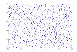
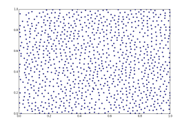
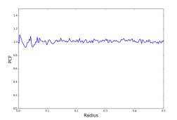
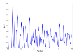
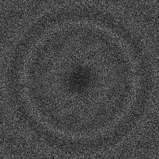
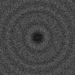
In this section we first provide a definition of a space-filling design. Subsequently, we propose a metric to quantify space-filling properties of sample designs.

3.1 Space-filling Designs

Without any prior knowledge of the function $f$ of interest, a reasonable objective when creating $\mathcal{X}$ is that the samples should be random to provide an equal chance of finding features of interest, e.g., local minima in an optimization problem, anywhere in $\mathcal{D}$. However, to avoid sampling only parts of the parameter space, a second objective is to cover the space in $\mathcal{D}$ uniformly, in order to guarantee that all sufficiently large features are found. Therefore, a good space-filling design can be defined as follows:

Definition 1

A space-filling design is a set of $\mathbf{x_{i}}$’s that are randomly distributed (Objective $1$: Randomness) but no two samples are closer than a given minimum distance $r_{min}$ (Objective $2$: Coverage).

Next, we describe the metric that we use to quantify the space-filling property of a sample design. The proposed metric is based on the spatial statistic, pair correlation function (PCF) and we will show that this metric is directly linked to an objective measure of design performance defined in the spectral domain.

3.2 Pair Correlation Function as a Space-filling Metric

In contrast to existing scalar space-filling metrics such as discrepancy, and coverage, the PCF characterizes the distribution of sample distances, thus providing a comprehensive description of the sample designs. More specifically, PCF describes the joint probability of having sampling points at a certain distance apart. A precise definition of the PCF can be given in terms of the intensity $\lambda$ and product density $\beta$ of a point process (Illian et al., 2008; Öztireli and Gross, 2012).

Definition 2

Let us denote the intensity of a point process $\mathcal{X}$ as $\lambda(\mathcal{X})$, which is the average number of points in an infinitesimal volume around $\mathcal{X}$. For isotropic point processes, this is a constant value. To define the product density $\beta$, let $\{B_{i}\}$ denote the set of infinitesimal spheres around the points, and $\{dV_{i}\}$ indicate the volume measures of $B_{i}$. Then, we have $P(\mathbf{x_{1}},\cdots,\mathbf{x_{N}})=\beta(\mathbf{x_{1}},\cdots,\mathbf{x_{N}})dV_{1}\cdots dV_{N}$. In the isotropic case, for a pair of points, $\beta$ depends only on the distance between the points, hence one can write $\beta(\mathbf{x_{i}},\mathbf{x_{j}})=\beta(||\mathbf{x_{i}}-\mathbf{x_{j}}||)=\beta(r)$ and $P(r)=\beta(r)dxdy$. The PCF is then defined as

$$G(r)=\dfrac{\beta}{\lambda^{2}}.$$ (1)

Note that, the PCF characterizes spatial properties of a sample design. However, in several cases, it is easier to link the objective performance of a sample design to its spectral properties. Therefore, we establish a connection between the spatial property of a sample design defined in PCF space to its spectral properties.

3.3 Connecting Spatial Properties and Spectral Properties of Space-filling Designs

Fourier analysis is a standard approach for understanding the objective properties of sampling patterns. Hence, we propose to analyze the spectral properties of sample designs, using tools such as the power spectral density, in order to assess their quality. For isotropic samples, a quality metric of interest is the radially-averaged power spectral density, which describes how the signal power is distributed over different frequencies.

Definition 3

For a finite set of $N$ points, $\{\mathbf{x}_{j}\}_{j=1}^{N}$, in a region with unit volume, the radially-averaged power spectral density (PSD) is formally defined as

$$P(k)=\frac{1}{N}|S(k)|^{2}=\frac{1}{N}\sum_{j,\ell}e^{-2\pi ik(\mathbf{x}_{\ell}-\mathbf{x}_{j})},$$ (2)

where $S(k)$ denotes the Fourier transform of the sample function.

Next, we show that the connection between spectral properties of a $d$-dimensional isotropic sample design and its corresponding pair correlation function can be obtained via the $d$-dimensional Fourier transform or more efficiently using the $1$-d Hankel transform.

Proposition 4

For an isotropic sample design with $N$ points, $\{\mathbf{x}_{j}\}_{j=1}^{N}$, in a $d$-dimensional region with unit volume, the pair correlation function $G(r)$ and radially averaged power spectral density $P(k)$ are related as follows:

$$G(r)=1+\dfrac{V}{2\pi N}H\left[P({k})-1\right]$$ (3)

where $V$ is the volume of the sampling region and $H[.]$ denotes the $1$-d Hankel transform, defined as

$$H(f(k))=\int_{0}^{\infty}kJ_{0}(kr)f(k)dk,$$

with $J_{0}(.)$ denoting the Bessel function of order zero.

Proof  Note that, PSD and PCF of a sample design are related via the $d$-dimensional Fourier transform as follows:

$$P(\mathbf{k}) = 1+\frac{N}{V}F\left(G(\mathbf{r})-1\right)$$

$$= 1+\frac{N}{V}\int_{\mathbb{R}^{d}}\left(G(\mathbf{r})-1\right)\exp(-i\mathbf{k.r})d\mathbf{r}.$$

It can be shown that, for radially symmetric or isotropic functions, the above relationship simplifies to

$$P(k)=1+2\pi\frac{N}{V}H\left[G({r})\right].$$

Next, using the inverse property of the Hankel transform, i.e.,

$$H_{0}^{-1}(f(r))=\int_{0}^{\infty}rJ_{0}(kr)f(r)dr,$$

we have

$$G(r)=1+\dfrac{V}{2\pi N}H\left[P({k})-1\right].$$ (4)

 
Proposition 4 is important as it enables us to qualitatively understand space-filling designs by first mapping them into the PCF space constructed based on spatial distances between points and, then, evaluating and understanding spectral properties of sample designs.

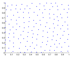
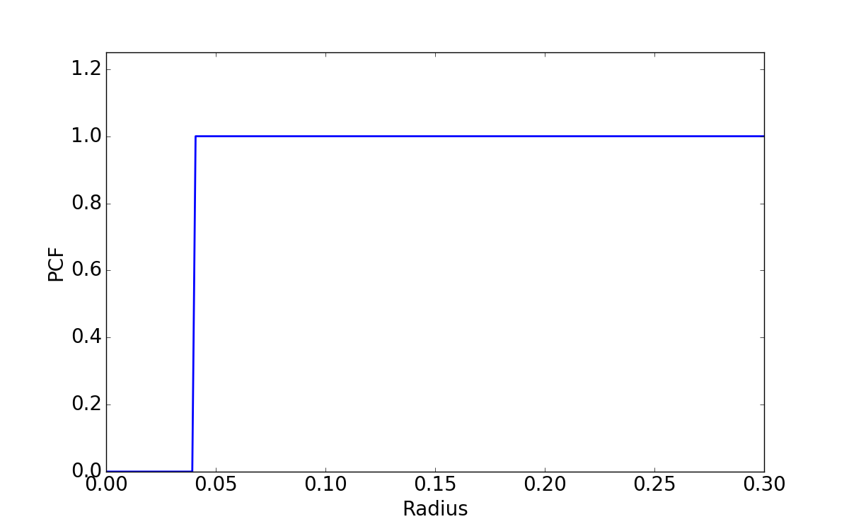
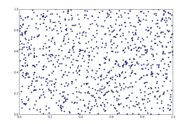
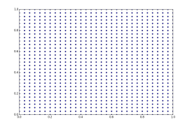
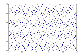
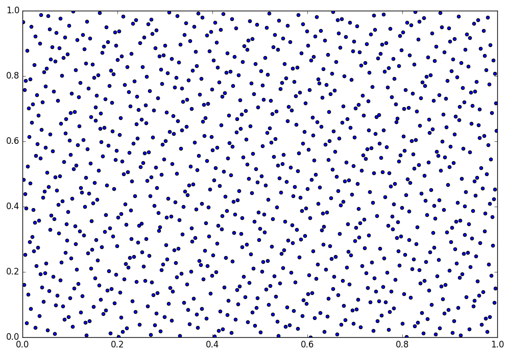
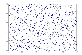
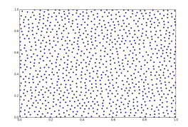
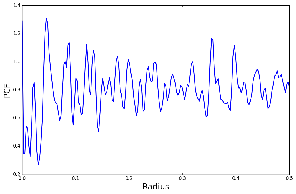
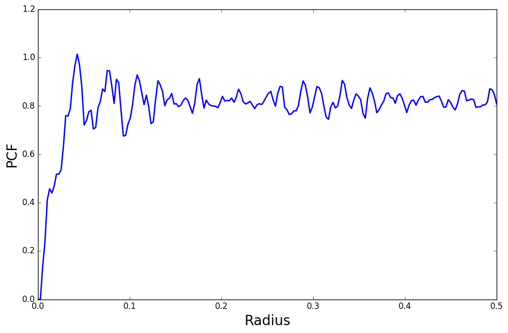
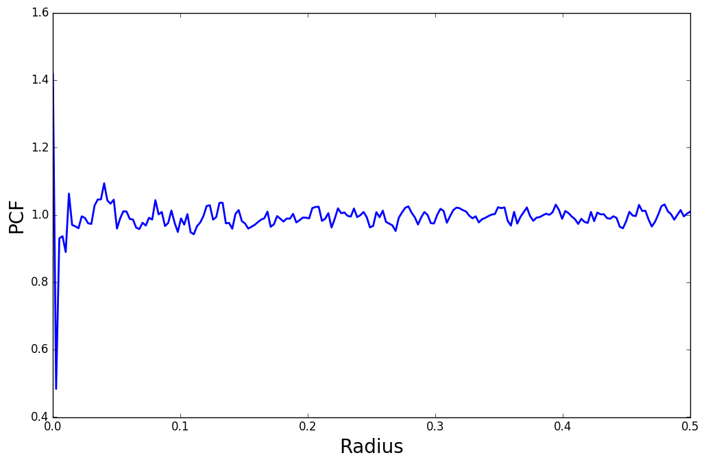
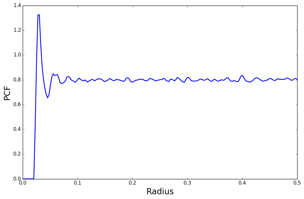
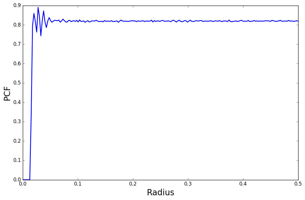
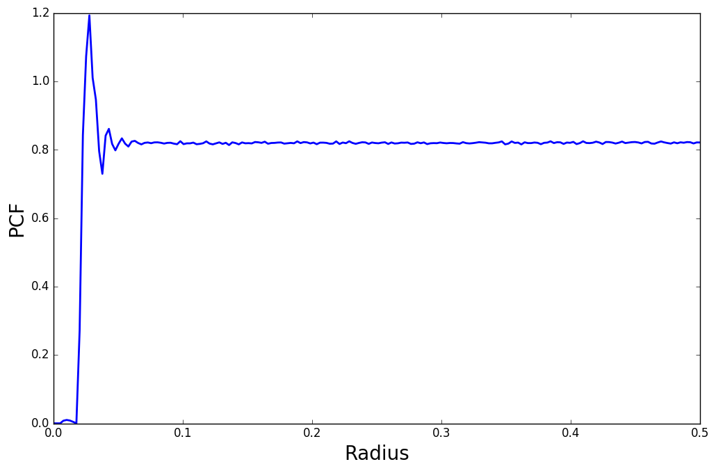
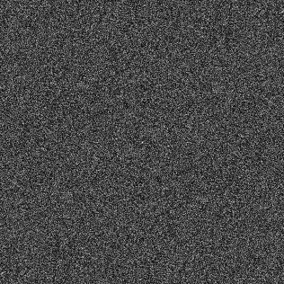
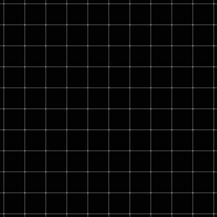
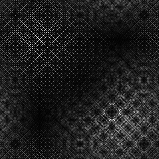
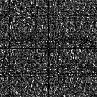
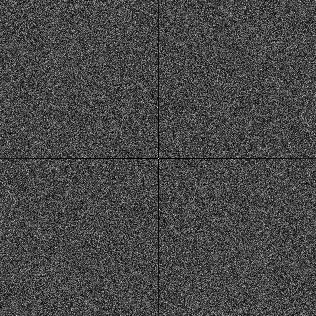
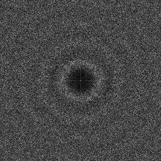
In Figure 3, we show the PCF of some commonly used $2$-d sample designs ($N=1000$) illustrated in Figure 2. As can be observed, both regular grid samples and QMC sequences have significant oscillations in their PCFs, which can be attributed to their structured nature. Regular grid sample design demonstrates a large disk radius $r_{min}$ ($G(r)=0$ for $0\leq r\leq r_{min}$) as every sample is at least $r_{min}$ apart from the rest of the samples, which in turn implies a better coverage. However, in practice, they perform poorly compared to randomized sample designs and this can be understood by studying their spectral properties. In contrast, random sample (Monte-Carlo) designs have a constant PCF with nearly no oscillations, since point samples are uncorrelated, thus, $P(r)=\lambda dx\lambda dy$ and theoretically have $G(r)=1,\;\forall r$. Furthermore, the LHS design has a similar PCF as random designs with the exception of a small, yet non-zero, $r_{min}$.

Other variants of PDS like MPDS, Step PCF and Stair PCF designs attempt to trade-off between coverage ($G(r)=0$ for $0\leq r\leq r_{min}$) and randomness $G(r)=1,\;\text{for}\;r>r_{min}$. Note that, the Step and the Stair PCF methods are space-filling spectral designs proposed later in this paper. However, upon a careful comparison, it can be seen that MPDS has a larger peak and more oscillations in its PCF compared to the proposed designs. In fact, our empirical studies show that the amount of oscillations in the PCF of the MPDS design significantly increases with dimensions.

Next, in Figure 4, we show the corresponding PSDs of the different sample designs. It can be seen that, oscillations in PCF directly correspond to oscillations in PSDs. For example, the oscillatory behavior of the PCF for regular and QMC sequences cause a non-uniform distribution of power in their corresponding PSDs. Furthermore, the larger peak height in the PCF of MPDS implies that a large amount of power is concentrated in a small frequency band instead of power being distributed over all frequencies. In Section 5, we will analyze the effect of the shape of PCF on the performance of a sample design in detail.

It is important to note that, not every PCF (or PSD) is physically realizable by a sample design. In fact, there are two necessary mathematical conditions  that a sample design must satisfy to be realizable.

Definition 5 (Realizability)

A PCF can be defined to be realizable through a sample design, if it satisfies the following conditions:

• its PCF must be non-negative, i.e., $G(r)\geq 0,\;\forall r$, and

• its corresponding PSD must be non-negative, i.e., $P(k)\geq 0,\;\forall k$.

As both the PSD and the PCF characteristics are strongly tied to each other (as shown in Proposition 4), these two conditions limit the space of realizable space-filling spectral designs. The results from this section will serve as tools for qualitatively understanding and, thus, designing optimal space-filling spectral designs in the following sections.

4 Space-filling Spectral Designs

In this section, we first formalize desired characteristics of a good space-filling design, as given in Definition 1. Next, we will describe the proposed framework for creating space-filling spectral designs.

Definition 6

A set of $N$ point samples $\mathcal{X}$ in a sampling domain $\mathcal{D}$ can be characterized as a space-filling design, if $\mathcal{X}=\{\mathbf{x_{i}}\in\mathcal{D};\;i=1,\cdots N\}$ satisfy the following two objectives:

• $\forall\mathbf{x_{i}}\in\mathcal{X},\;\forall\triangle\mathcal{D}\subseteq\mathcal{D}\;:\;P(\mathbf{x_{i}}\in\triangle\mathcal{D})=\int_{\triangle\mathcal{D}}\mathbf{dx}$

• $\forall\mathbf{x_{i}},\mathbf{x_{j}}\in\mathcal{X}\;:\;||\mathbf{x_{i}}-\mathbf{x_{j}}||\geq r_{\text{min}}$

where $r_{\text{min}}$ is referred to as the coverage radius.

In the above definition, the first objective states that the probability of a uniformly distributed random sample $\mathbf{x_{i}}\in\mathcal{X}$ falling inside a subset $\triangle\mathcal{D}$ of $\mathcal{D}$ is equal to the hyper-volume of $\triangle\mathcal{D}$. The second condition enforces the minimum distance constraint between point sample pairs for improving coverage.

A Poisson design enforces the first condition alone, in which case the number of samples that fall inside any subset $\triangle\mathcal{D}\subseteq\mathcal{D}$ obeys a discrete Poisson distribution. Though easier to implement, Poisson sampling often produces distributions where the samples are grouped into clusters and leaves holes in possibly the regions of interest. In other words, this increases the risk of missing important features, when only the samples are used for analysis. Consequently, a sample design that distributes random samples in a uniform manner across $\mathcal{D}$ is preferred, so that clustering patterns are not observed. The coverage condition explicitly eliminates the clustering behavior by preventing samples from being closer than $r_{\text{min}}$. A space-filling design can be defined conveniently in the PCF domain and we refer to this as the space-filling spectral design, due to its direct connection to the spectral domain properties.

4.1 Defining a Space-filling Spectral Design in Spatial Domain

For Poisson design, point locations are not correlated and, therefore, $P(r)=\lambda dx\lambda dy$. This implies that for Poisson designs $G(r)=1$. Similarly, for space-filling designs, due to the minimum distance constraint between the point sample pairs, we do not have any point samples in the region $0\leq r<r_{\text{min}}$. Consequently, space-filling spectral designs are defined as a step pair correlation function in the spatial domain (Step PCF).

Proposition 7

Given the desired coverage radius $r_{\text{min}}$, a space-filling spectral design is defined in the spatial domain as

$$G(r-r_{\text{min}})=\left\{\begin{array}[]{rll}0&\mbox{if}\ r<r_{\text{min}}\\ 1&\mbox{if}\ r\geq r_{\text{min}}.\end{array}\right.$$

As a consequence of Proposition 4, space-filling spectral designs can equivalently be defined in the spectral domain.

4.2 Defining a Space-filling Spectral Design in Spectral Domain

We derive the power spectral density of the space-filling spectral design using the connection established in Section 3. Following our earlier notation, we denote the $d$-dimensional power spectral density by $P(\mathbf{k})$ and $d$-dimensional PCF by $G(\mathbf{r})$.

Proposition 8

Given the desired coverage radius $r_{\text{min}}$, a $d$-dimensional space-filling spectral design $\mathcal{X}$, with $N$ sample points in a sampling domain $\mathcal{D}$ of volume $V$, can be defined in the PSD domain as

$$P(k)=1-\frac{N}{V}\left(\dfrac{2\pi r_{\text{min}}}{k}\right)^{\frac{d}{2}}J_{\frac{d}{2}}(kr_{\text{min}})$$

where $J_{\frac{d}{2}}(.)$ is the Bessel function of order $d/2$.

Proof  We know that,

$$P(\mathbf{k}) = 1+\frac{N}{V}F\left(G(\mathbf{r})-1\right),$$ (5)

$$= 1+\frac{N}{V}\int_{\mathbb{R}^{d}}\left(G(\mathbf{r})-1\right)\exp(-i\mathbf{k.r})d\mathbf{r},$$ (6)

where $F(.)$ denotes the $d$-dimensional Fourier transform. Note that, for the radially symmetric or isotropic functions, i.e., $G(r)$ where $r=||\mathbf{r}||$, the above relationship simplifies to

$$P(k)=1+\frac{N}{V}\;{(2\pi)^{\frac{d}{2}}}k^{1-\frac{d}{2}}H_{\frac{d}{2}-1}\left(r^{\frac{d}{2}-1}(G({r})-1)\right),$$ (7)

where

$$H_{v}(f(r))(k)=\int_{0}^{\infty}rJ_{v}(kr)f(r)dr$$

is the $1-$d Hankel transform of order $v$ with $J$ being the Bessel function. To derive the PSD of a step function, we first evaluate the Hankel transform of $f(r)=(G(r)-1)$ where $G(r)$ is a step function.

$$H_{\frac{d}{2}-1}\left(r^{\frac{d}{2}-1}(G(r)-1)\right) = \int_{0}^{\infty}r^{\frac{d}{2}}J_{\frac{d}{2}-1}(kr)\left(G(r)-1\right)dr$$

$$= -\int_{0}^{r_{\text{min}}}r^{\frac{d}{2}}J_{\frac{d}{2}-1}(kr)dr$$

$$= -\dfrac{{}^{r_{\text{min}}^{\frac{d}{2}}}}{k}J_{\frac{d}{2}}(kr_{\text{min}})$$

Using this expression in (7), we obtain

$$P(k)=1-\frac{N}{V}\left(\dfrac{2\pi r_{\text{min}}}{k}\right)^{\frac{d}{2}}J_{\frac{d}{2}}(kr_{\text{min}}).$$ (8)

 
This proposition connects the spatial properties of a space-filling spectral design, defined via the PCF, to its spectral properties. The motivation for this is the fact that in several cases, it is easier to link the objective performance of a sample design to its spectral properties. In the next section, we will develop the relation between spectral properties and an objective measure of the performance, which in turn provides us guidelines for designing better space-filling spectral sampling patterns.

5 Qualitative Analysis of Space-filling Spectral Designs

In this section, we derive insights regarding the objective performance of space-filling spectral designs. To this end, we analyze the impact of the shape of the PCF on the reconstruction performance. Further, for a tractable analysis, we consider the task of recovering the class of periodic functions using space-filling spectral designs and analyze the reconstruction error as a function of their spectral properties. The analysis presented in this section will clarify how the shape of the PCF of a sample design directly impacts its reconstruction performance.

5.1 Analysis of Reconstruction Error for Periodic Functions

Let us denote the Fourier transform of the sample design $\mathcal{X}$ by $\mathcal{S}$. The function to be sampled and its corresponding Fourier representation are denoted by $\mathcal{I}$ and $\hat{\mathcal{I}}(k)$ respectively. Now, the spectrum of the sampled function is given by $\hat{\mathcal{I}}_{s}(k)=\mathcal{S}\ast\hat{\mathcal{I}}(k)$. Note that, a sampling pattern with a finite number of points is comprised of two components, a DC peak at the origin and a noisy remainder $\mathcal{\bar{S}}$. Thus, equivalently, we have $\hat{\mathcal{I}}_{s}(k)=\{n\delta(k)+\mathcal{\bar{S}}\}\ast\hat{\mathcal{I}}(k).$ The error introduced in the process of function reconstruction is the difference between the reconstructed and the original functions:

$$\mathcal{E}(k)=|\hat{\mathcal{I}}_{s}(k)/N-\mathcal{I}(k)|^{2}=|\mathcal{\bar{S}}\ast\hat{\mathcal{I}}(k)/N|^{2}$$

where we have divided the R.H.S. by $N$ to normalize the energy of $\mathcal{I}_{s}$. For error analysis, we focus on the low frequency content of the error term, since the high frequency components are removed during the reconstruction process.

Denoting the power spectrum without the DC component by $\mathcal{P^{\prime}}(k)$, for a constant function the error simplifies to

$$\mathcal{E}(k)\propto|\mathcal{S^{\prime}}(k)|^{2}\propto\mathcal{P^{\prime}}(k).$$ (9)

This, as stated above, allows for the characterization of the error in terms of the spectral properties of the sampling pattern used.

Next, we consider an important class of functions, the family of periodic functions, for further analysis. All periodic functions with a finite period can be expressed as a Fourier series, which is a summation of sine and cosine terms

$$\mathcal{I}(x)=a_{0}+\sum_{m=1}^{M}a_{m}cos(2\pi mx)+\sum_{m=1}^{M}b_{m}sin(2\pi mx).$$

The Fourier transform of this function is equivalently a summation of pulses:

$$\hat{\mathcal{I}}(k)=a_{0}\delta(k)+\sum_{m=1}^{M}a_{m}\left(\dfrac{1}{2}(\delta(k-m)+\delta(k+m)\right)+\sum_{m=1}^{M}b_{m}\left(\dfrac{1}{2}(\delta(k+m)-\delta(k-m))\right).$$

Making substitutions, $a_{m}+b_{m}=A_{m},a_{m}-b_{m}=B_{m}$, we obtain

$$\mathcal{E}(k)=\dfrac{1}{4N^{2}}\Big{|}4a_{0}\mathcal{S^{\prime}}(k)+\sum_{m=1}^{M}\big{(}A_{m}\mathcal{S^{\prime}}(k+m)+B_{m}\mathcal{S^{\prime}}(k-m)\big{)}\Big{|}^{2}.$$

The reconstruction error can then be upper bounded as follows:

$$\mathcal{E}(k)\leq\dfrac{1}{4N}\Big{[}4a_{0}^{2}\mathcal{P^{\prime}}(k)+\sum_{m=1}^{M}\big{(}A_{m}^{2}\mathcal{P^{\prime}}(k+m)+B_{m}^{2}\mathcal{P^{\prime}}(k-m)\big{)}\Big{]}.$$ (10)

In the case of a single sinusoidal function, $cos(2\pi fx)$, using triangle inequality, this becomes (Heck et al., 2013)

$$\mathcal{E}(k)\leq\dfrac{1}{4N}\Big{[}\mathcal{P^{\prime}}(k+f)+\mathcal{P^{\prime}}(k-f)+2\;\sqrt[]{\mathcal{P^{\prime}}(k+f)\mathcal{P^{\prime}}(k-f)}\Big{]}.$$ (11)

Even though this is only an upper bound, we will see that it accurately predicts the characteristics of the sampling error and provides useful guidelines.

The above analysis implies that to assess the quality of the sample designs, one can analyze their spectral behavior. More specifically, the above analysis suggests that to minimize the reconstruction error: (a) the power spectra of the sample design should be close to zero, and (b) for errors to be broadband white noise (uniform over frequencies), the power spectra should be a constant. Note that, in several applications, e.g., image reconstruction, most relevant information is predominantly at low frequencies. In such scenarios, this naturally leads to the following criteria for sample designs: (a) the spectrum should be close to zero for low frequencies which indicates the range of frequencies that can be represented with almost no error, (b) the spectrum should be a constant for high frequencies or contain minimal amount of oscillations in the power spectrum.

5.2 Effect of PCF Characteristics on Sampling Performance

Based on the two criteria discussed above, we assess the effect of the shape of the PCF on the quality of space-filling designs in the spectral domain. Note that, PCFs of the samples constructed in practice (Figure 2) often demonstrates the following characteristics: (a) presence of a zero-region characterized by $r_{min}$, (b) a large peak around $r_{min}$, and (c) damped oscillations. To model and analyze these characteristics, we consider the following parametric PCF family:

$$G(r)=G(r-r_{\text{min}})+a\left(G(r-r_{\text{min}})-G(r-r_{\text{min}}-\delta)\right)$$ (12)

$$\qquad+\frac{a}{4r}\exp(-r/2)\sin(c\times r-c)G(r-r_{\text{min}})$$

where $G(r-r_{\text{min}})$ is the Step function, peak width $\delta\geq 0$ and the peak height $a\geq 1$ and last term in (12) corresponds to damped oscillations. This family is a generalization of Step PCF, with additional parameterization of peak height and oscillations in the PCF.

5.2.1 Effect of Peak Height on Spectral Properties

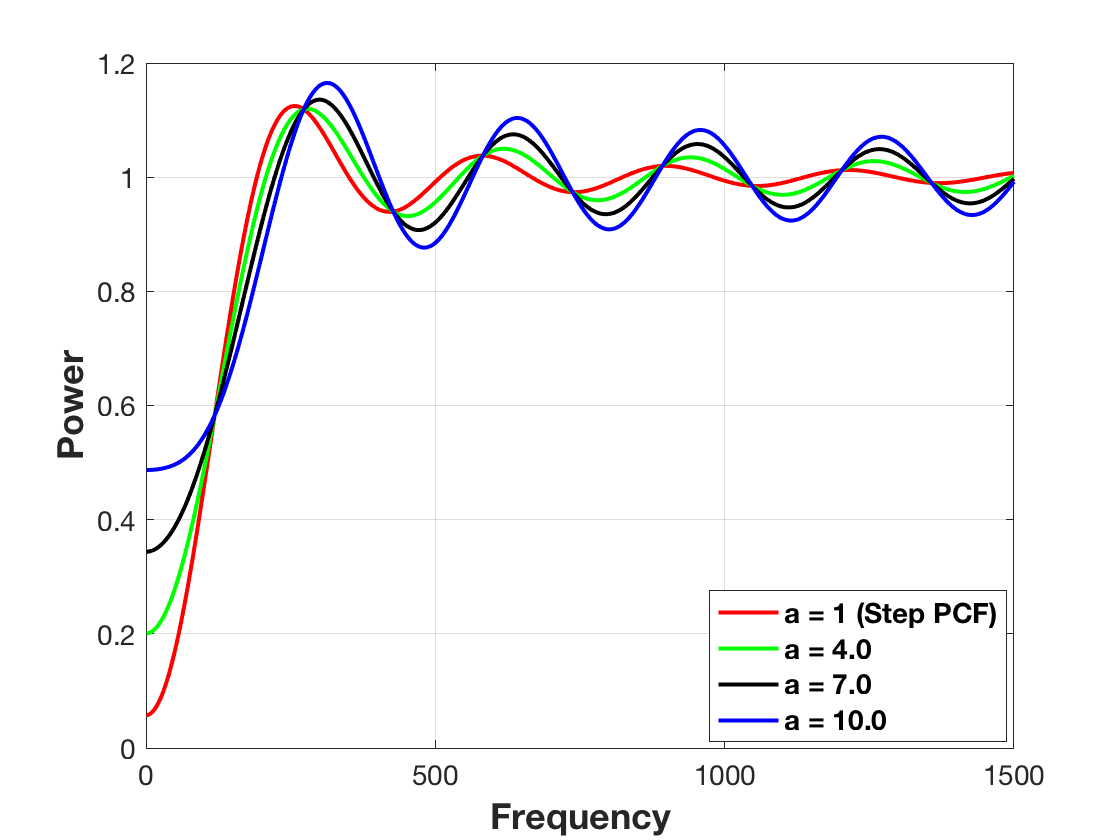
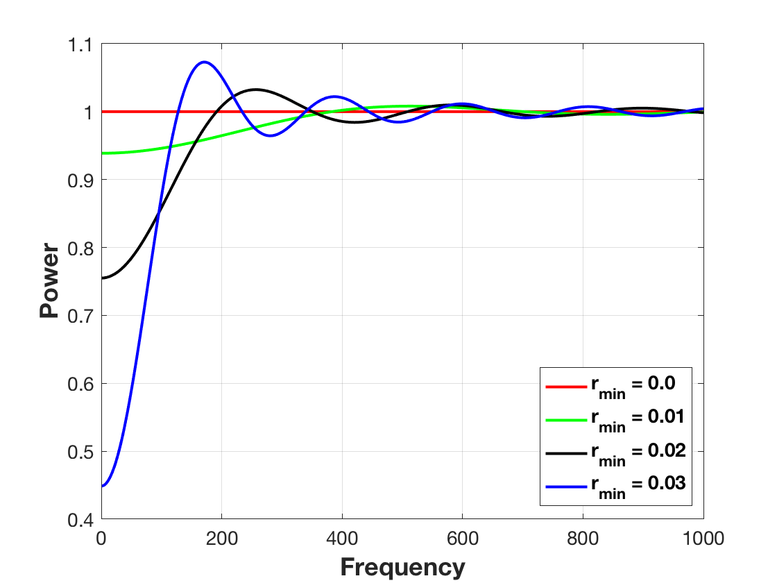
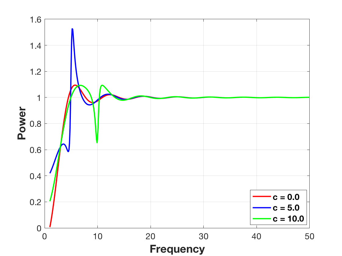
In order to study the impact of increasing peak height in the PCF on the PSD characteristics, we conduct an empirical study. We compute the PSD of a sample design with the following parameters: $N=195,r_{\text{min}}=0.02,\delta=0.005$. Note that, we vary the PCF peak height $a$, which actually reflects the behavior of existing coverage based PDS algorithms. As shown in Figure 5, increasing $a$ results in both significantly higher low frequency power and larger high frequency oscillations. As expected, the PSD of the Step PCF (or $a=1$) performs the best, i.e., the spectrum is close to zero for low frequencies and constant for high frequencies.

5.2.2 Effect of Disk Radius on Spectral Properties

Next, we study the importance of choosing an appropriate $r_{\text{min}}$ (or coverage $\rho$) while generating sample distributions. In Figure 5, we show the PSD for $N=195$ and $a$ = 1, with varying disk radius values $r_{\text{min}}$. For a fixed sample budget, as we increase the radius, we observe two contrasting changes in the PSD: $(i)$ the spectrum tends to be close to zero at low frequencies and $(ii)$ an increase in oscillations for high frequencies. Consequently, there is a trade-off between low frequency power and high frequency oscillations in power spectra which can be controlled by varying $r_{\text{min}}$. However, the increase in oscillations are less significant compared to the gain in the zero-region. Furthermore, in several applications, low frequency content is more informative, and hence one may still attempt to maximize $r_{min}$ or coverage.

5.2.3 Effect of Oscillations on Spectral Properties

Finally, we study the effect of oscillations in the PCF on the power distribution in the spectral domain. In Figure 5, we plot the PSD for $a=1$ with varying amounts of oscillations controlled via the parameter $c$. It can be seen that introducing oscillations in the PCF results in significantly higher low frequency power and larger high frequency oscillations. As expected, the PSD of the Step PCF (or $c=0$) behaves the best.

In summary, the discussion in this section suggests that the PCF of an ideal space-filling spectral design should have the following three properties: $(a)$ large $r_{min}$, $(b)$ small peak height, and $(c)$ low oscillations. Since, the Step PCF satisfies these three properties, it is expected to be a good space-filling spectral design. Next, we consider the problem of optimizing the parameter of the Step PCF design, i.e. $r_{min}$.

Figure 5: (a) Effect of peak height in the PCF on power spectra, (b) Effect of disk radius in the PCF on power spectra, (c) Effect of oscillations in the PCF on power spectra.

6 Optimization of Step PCF based Space-filling Spectral Designs

The proposed space-filling metric enjoys mathematical tractability and is supported by theoretical results as defined in Section 4. This enables us to obtain new insights for optimizing Step PCF based space-filling spectral designs. In particular, (a) For a fixed $r_{\text{min}}$, we obtain the maximum number of point samples in any arbitrary dimension $d$, (b) For a fixed sampling budget $N$, we derive the maximum achievable $r_{\text{min}}$ in arbitrary dimension $d$.

6.1 Case 1: Fixed $r_{\text{min}}$

The problem of finding the maximum number of point samples in a Step PCF based space-filling spectral design with a given disk radius $r_{\text{min}}$ can be formalized as follows:

$$\begin{split}{\mathrm{maximize}}\quad&N\\ \mbox{subject to}\quad&P(k)\geq 0,\;\forall k\\ \quad&G(r-r_{\text{min}})\geq 0,\;\forall r,\end{split}$$ (13)

where $P(k)=1-\frac{N}{V}\left(\dfrac{2\pi r_{\text{min}}}{k}\right)^{\frac{d}{2}}J_{\frac{d}{2}}(kr_{\text{min}})$. Note that, a space-filling spectral design has to satisfy realizability constraints as defined in Definition 5.

Proposition 9

For a fixed disk radius $r_{\text{min}}$, the maximum number of point samples possible for a realizable Step PCF based space-filling spectral design in the sampling region with volume $V$ is given by

$$N=\dfrac{V\Gamma\left(\frac{d}{2}+1\right)}{\pi^{\frac{d}{2}}r_{\text{min}}^{d}}.$$

Proof  Using the definition of the Step PCF function, the constraint $G(r-r_{\text{min}})$ is trivially satisfied. Note that, the constraint $P(k)\geq 0,\;\forall k$ is equivalent to $\underset{k}{\min}\;P(k)\geq 0$. In other words,

$$\underset{k}{\min}\;1-\rho\left(\dfrac{2\pi r_{\text{min}}}{k}\right)^{\frac{d}{2}}J_{\frac{d}{2}}(kr_{\text{min}})\geq 0$$

$$\Leftrightarrow \underset{k}{\max}\;\rho\left(\dfrac{2\pi r_{\text{min}}}{k}\right)^{\frac{d}{2}}J_{\frac{d}{2}}(kr_{\text{min}})\leq 1$$

$$\Leftrightarrow \rho\left({2\pi}\right)^{\frac{d}{2}}r_{\text{min}}^{d}\;\underset{k}{\max}\;\left(\dfrac{J_{\frac{d}{2}}(kr_{\text{min}})}{(kr_{\text{min}})^{\frac{d}{2}}}\right)\leq 1$$

$$\Leftrightarrow \rho\left({2\pi}\right)^{\frac{d}{2}}r_{\text{min}}^{d}\;\dfrac{1}{2^{\frac{d}{2}}\Gamma\left(\frac{d}{2}+1\right)}\leq 1$$

$$\Leftrightarrow N\leq\dfrac{V\Gamma\left(\frac{d}{2}+1\right)}{\left({\pi}\right)^{\frac{d}{2}}r_{\text{min}}^{d}}$$

where, we have used the fact that $J_{v}(x)\approx{(x/2)^{v}}/{\Gamma(v+1)}$.  

Note that, for the $2$-dimensional case, we have $\frac{J_{1}(kr_{\text{min}})}{kr_{\text{min}}}=\text{jinc}(kr_{\text{min}})$. Now using the fact that $\text{jinc}(x)$ has the maximum value equal to $1/2$, for a fixed disk radius $r_{\text{min}}$, the maximum number of point samples possible in a $2$-d Step PCF based space-filling spectral design is given by

$$N={V}/{\pi(r_{\text{min}})^{2}},$$

which again corroborates our bound in Proposition 9.

6.2 Case 2: Fixed $N$

Alternately, we can also derive the bound for the disk radius of Step PCF with a fixed sampling budget $N$ as follows:

$$\begin{split}{\mathrm{maximize}}\quad&r_{\text{min}}\\ \mbox{subject to}\quad&P(k)\geq 0,\;\forall k\\ \quad&G(r-r_{\text{min}})\geq 0,\;\forall r\end{split}$$ (14)

Proposition 10

For a fixed sampling budget $N$, the maximum possible disk radius $r_{\text{min}}$ for a realizable Step PCF based space-filling spectral design in the sampling region with volume $V$ is given by

$$r_{\text{min}}=\sqrt[d]{\dfrac{V\Gamma\left(\frac{d}{2}+1\right)}{\pi^{\frac{d}{2}}N}}.$$

Proof  The proof is similar to the one in Proposition 9.  

6.3 Relative Radius of Step PCF

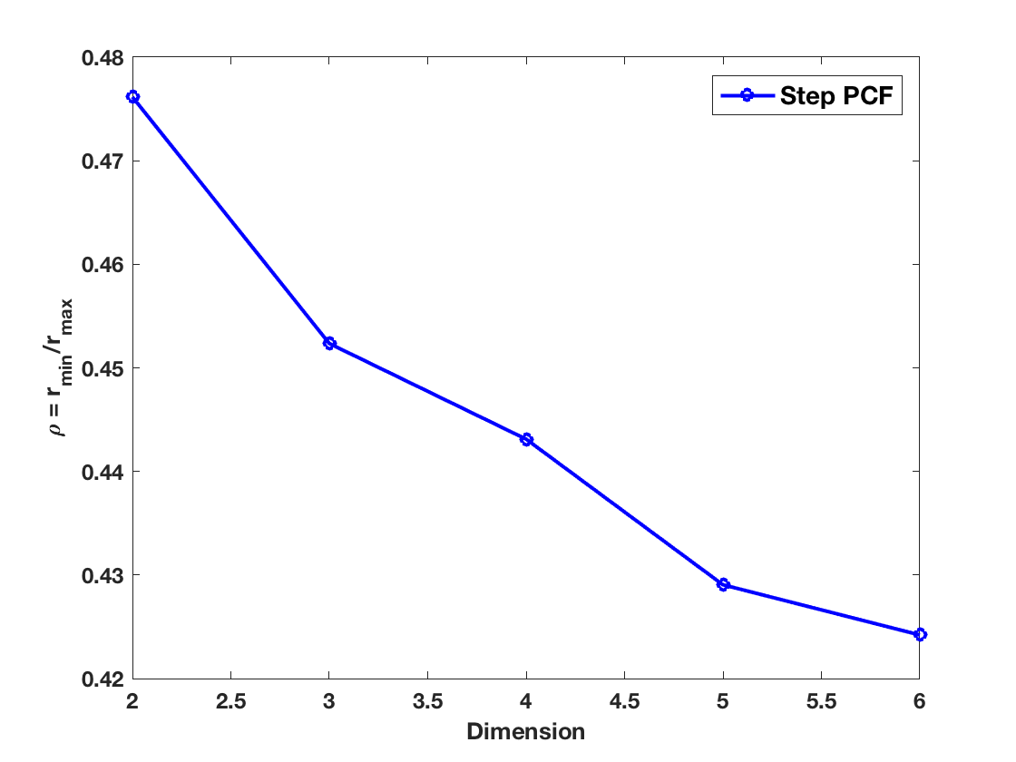
As mentioned before, the current literature characterizes coverage by the fraction $\rho$ of the maximum possible radius $r_{max}$ for $N$ samples to cover the sampling domain, such that $r_{min}=\rho r_{max}$. The maximum possible disk radius is achieved by the deterministic hexagonal lattice (Schreiber, 1943) and can be approximated in a $d$ dimensional sampling region as $r_{max}\approx\sqrt[d]{\tfrac{A_{d}}{C_{d}N}}$. Here, $A_{d}$ is the hypervolume of the sampling domain and $C_{d}=V_{d}/r^{d}$ with $V_{d}$ being the hypervolume of a hypersphere with radius $r$. Note that, a uniformly distributed point set can have a relative radius of $0$, and the relative radius of a hexagonal lattice equals $1$ (in $2$-d). Next, we derive a closed-form expression for the relative radius of Step PCF based design.

Proposition 11

For a fixed sampling budget $N$, the maximum relative radius $\rho$ for Step PCF based space-filling spectral design in the sampling region with volume $V$ is given by $\rho=\dfrac{1}{2\;\sqrt[d]{\eta_{d}}}$ where $\eta_{d}$ is maximal density of a sphere packing in $d$-dimensions.

Proof  Let us denote by $r_{max}=\underset{r}{\arg\min}\;\eta_{d}$, then, the maximal density of a sphere packing with $N$ samples in $d$-dimensions is given by

$$\eta_{d}=\dfrac{N\pi^{d/2}}{\Gamma(1+\frac{d}{2})}\dfrac{r_{max}^{d}}{V}$$ (15)

$$\Leftrightarrow \eta_{d}=\left(\frac{r_{max}}{r_{min}}\right)^{d}$$ (16)

$$\Leftrightarrow \rho=\dfrac{1}{2\;\sqrt[d]{\eta_{d}}}$$ (17)

where equality in (16) uses Proposition (10).  

For $d=2$ and $3$, the relative radius simplifies to:

$$\rho=0.5\sqrt[2]{\dfrac{\pi\sqrt{3}}{6}},\;\textbf{for}\;d=2,\;\text{and}$$

$$\rho=0.5\sqrt[3]{\dfrac{\pi\sqrt{2}}{6}},\;\textbf{for}\;d=3.$$

Note that, finding the maximal density of a sphere packing for an arbitrary high dimension (except in $d=2,3$ and recently in $8,24$ (viazovska, 2017; Cohn et al., 2017)) is an open problem. Note that, best known packings are often lattices, thus, we use the best known lattices to be an approximation of $r_{max}$ in our analysis.

In Figure 6, we plot the relative radius $\rho=r_{min}/r_{max}$ of Step PCF for different dimensions $d$. It is interesting to notice that the relative radius of Step PCF based designs increases as the dimension $d$ increases, i.e., Step PCF based designs approach a more regular pattern. Further, note that, for a fixed sampling budget both $r_{min}$ and $r_{max}$ increase as the number of dimensions increases. The Step PCF based designs maintain randomness by keeping the PCF flat, but this comes at a cost: the disk radius $r_{min}$ of these patterns is very small (as can be seen from Figure 6). For several applications, covering the space better (by trading-off randomness) is more important. In the next section, we will propose a new class of space-filling spectral designs that can achieve a much higher $r_{min}$ at the small cost of compromising randomness by introducing a single peak into an otherwise flat PCF.

Figure 6: Relative radius $\rho=r_{min}/r_{max}$ of Step PCF based space-filling spectral design for different dimensions $d$.

7 Space-filling Spectral Designs with Improved Coverage

To improve the coverage of Step PCF base space-filling spectral design, in this section, we propose a novel space-filling spectral design which systematically trades-off randomness with coverage of the resulting samples. Note that, the randomness property can be relaxed either by increasing the peak height of the PCF, or by increasing the amounts oscillations in the PCF (as discussed in Section 5.2). For simplicity, we adopt the former strategy and use only the peak height parameter. More specifically, as an alternative to Step PCF, we design the following generalization which we refer as the Stair PCF design.

7.1 Stair PCF based Space-filling Spectral Design

Now, we define the proposed Stair PCF based space-filling design and quantify the gains achieved in the coverage characteristics (i.e. $r_{min}$).

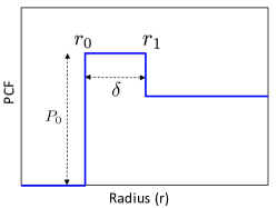
Stair PCF in the Spatial Domain: The Stair PCF construction is defined as follows:

$$G(r;r_{0},r_{1},P_{0})=f(r-r_{1})+P_{0}\left(f(r-r_{0})-f(r-r_{1})\right),$$ (18)

$$\text{with }f(r-r_{0})=\left\{\begin{array}[]{rll}0&\mbox{if}\ r\leq r_{0}\\ 1&\mbox{if}\ r>r_{0}\end{array}\right\},$$ (21)

$$\text{where }r_{0}\leq r_{1}\text{ and }P_{0}\geq 1.$$

This family of space-filling spectral designs has three interesting properties:

• except for a single peak in the region $r_{0}\leq r\leq r_{1}$, the PCF is flat, thus, does not compromise randomness entirely,

• both the height and width of the peak can be optimized to maximize coverage,

• the Step PCF based spectral design can be derived as as a special case of this construction.

A representative example of Stair PCF is shown in Figure (7).

Stair PCF in the Spectral Domain: Following the analysis in the earlier sections, we derive the power spectral density of Stair PCF based space-filling spectral designs.

Proposition 12

The power spectral density of a Stair PCF based space-filling spectral designs, $G(r;r_{0},r_{1},P_{0})$, with $N$ samples in the sampling region with volume $V$ is given by

$$P(k)=1-\frac{N}{V}P_{0}\left(\dfrac{2\pi r_{0}}{k}\right)^{\frac{d}{2}}J_{\frac{d}{2}}(kr_{0})-\frac{N}{V}(1-P_{0})\left(\dfrac{2\pi r_{1}}{k}\right)^{\frac{d}{2}}J_{\frac{d}{2}}(kr_{1}).$$

Proof  Using results from Section 4.2, we have

$$P(k)=1+\frac{N}{V}\;{(2\pi)^{\frac{d}{2}}}k^{1-\frac{d}{2}}H_{\frac{d}{2}-1}\left(r^{\frac{d}{2}-1}(G({r})-1)\right).$$ (22)

To derive the PSD of a Stair function, we first evaluate the Hankel transform of $f(r)=(G(r)-1)$ where $G(r)$ is a Stair function.

$$H_{\frac{d}{2}-1}\left(r^{\frac{d}{2}-1}(G(r)-1)\right)=\int_{0}^{\infty}r^{\frac{d}{2}}J_{\frac{d}{2}-1}(kr)\left(G(r)-1\right)dr$$

$$=-P_{0}\int_{0}^{r_{0}}r^{\frac{d}{2}}J_{\frac{d}{2}-1}(kr)dr-(1-P_{0})\int_{0}^{r_{1}}r^{\frac{d}{2}}J_{\frac{d}{2}-1}(kr)dr$$

$$=-P_{0}\dfrac{{}^{r_{0}^{\frac{d}{2}}}}{k}J_{\frac{d}{2}}(kr_{0})-(1-P_{0})\dfrac{{}^{r_{1}^{\frac{d}{2}}}}{k}J_{\frac{d}{2}}(kr_{1})$$

Using this expression in (22),

$$P(k)=1-\frac{N}{V}P_{0}\left(\dfrac{2\pi r_{0}}{k}\right)^{\frac{d}{2}}J_{\frac{d}{2}}(kr_{0})-\frac{N}{V}(1-P_{0})\left(\dfrac{2\pi r_{1}}{k}\right)^{\frac{d}{2}}J_{\frac{d}{2}}(kr_{1}).$$ (23)

 

(a) $d=2$

(b) $d=3$

(c) $d=4$

(d) $d=5$

(e) $d=6$

Figure 7: (a) Pair correlation function of Stair PCF based designs, (b)-(f) Maximum Disk Radius For Step and Stair PCF for dimensions $2$ to $6$.

Next, we empirically evaluate the gain in coverage achieved by Stair PCF based designs compared to the Step PCF based designs.

7.2 Coverage Gain with Stair PCF

Ideally, the optimal Stair PCF should be obtained by simultaneously maximizing $r_{0}$ ($:=r_{min}$) and minimizing $P_{0}$. Furthermore, not all PCFs in the Stair PCF family are realizable. Due to the realizability conditions, the parameters cannot be adjusted independently. The main challenge, therefore, is to find the combinations of the three parameters $(r_{0},r_{1},P_{0})$ that is realizable and yield a good sample design. Unlike Step PCF, the closed form expression for the optimal parameters $(r_{0},r_{1},P_{0})$ are difficult to obtain, and, therefore, we explore this family of PCF patterns empirically by searching configurations for which:

• the disk radius $r_{0}$ is as high as possible, and

• the PCF is flat with minimal increase in the peak height $P_{0}$.

7.2.1 Disk Radius $r_{min}$ vs. Sample Budget $N$

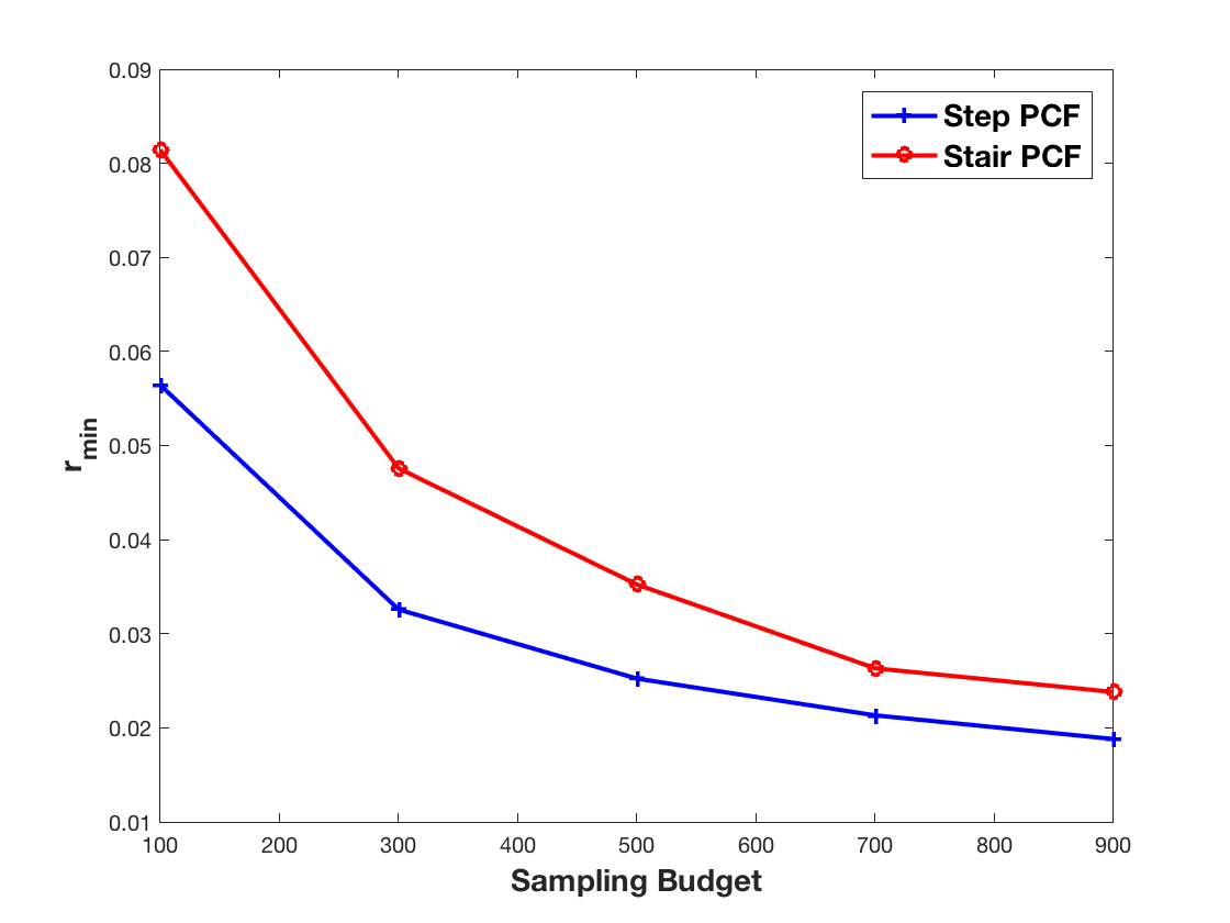
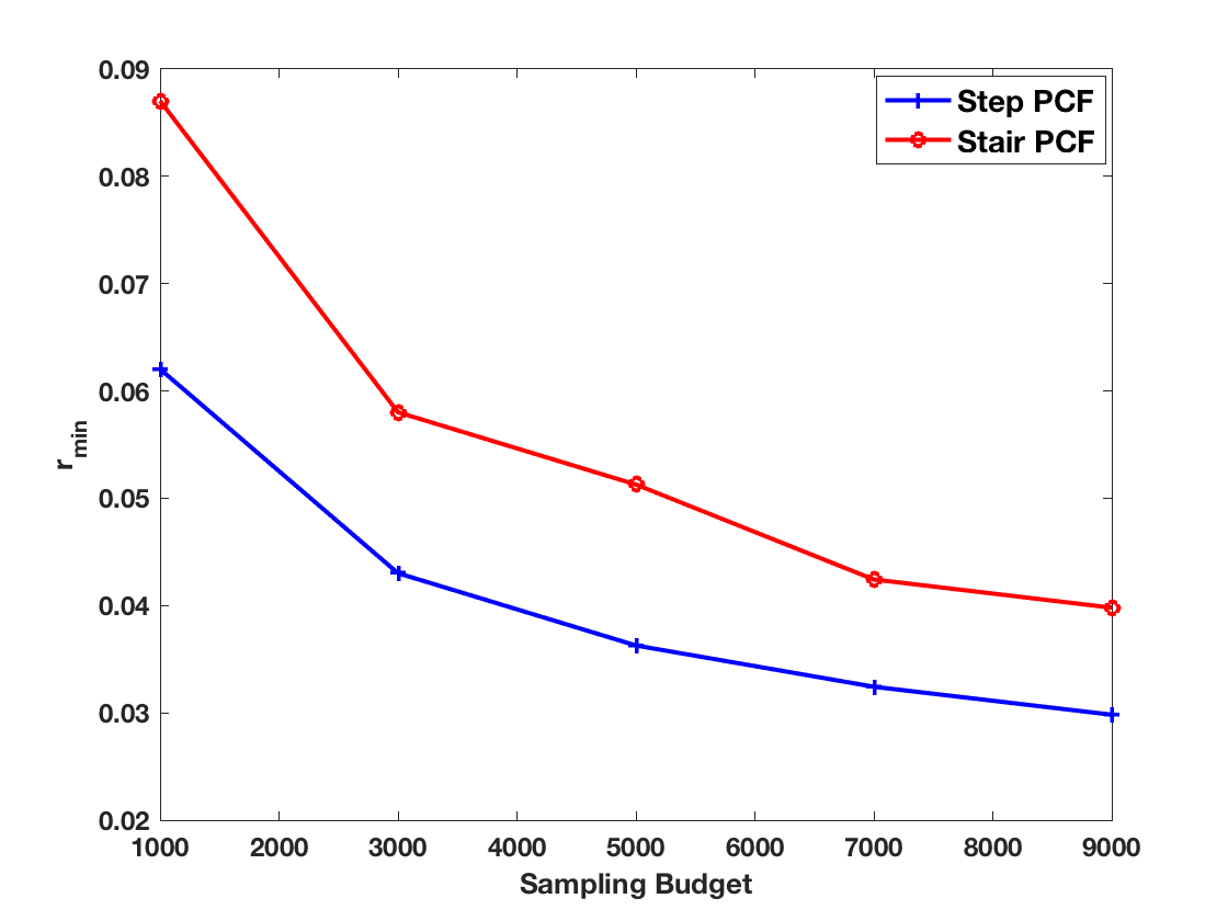
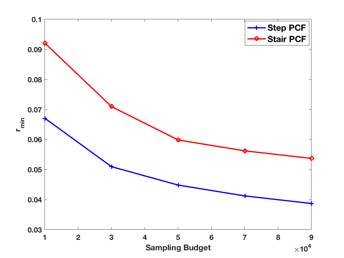
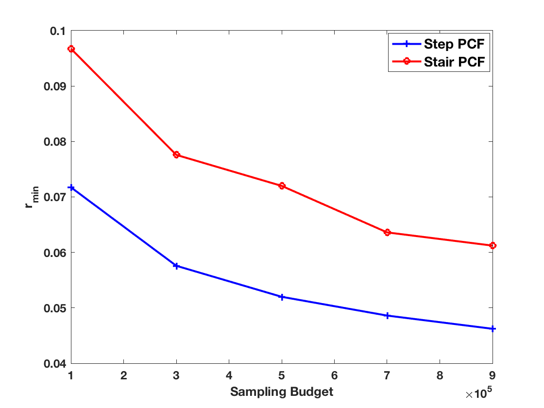
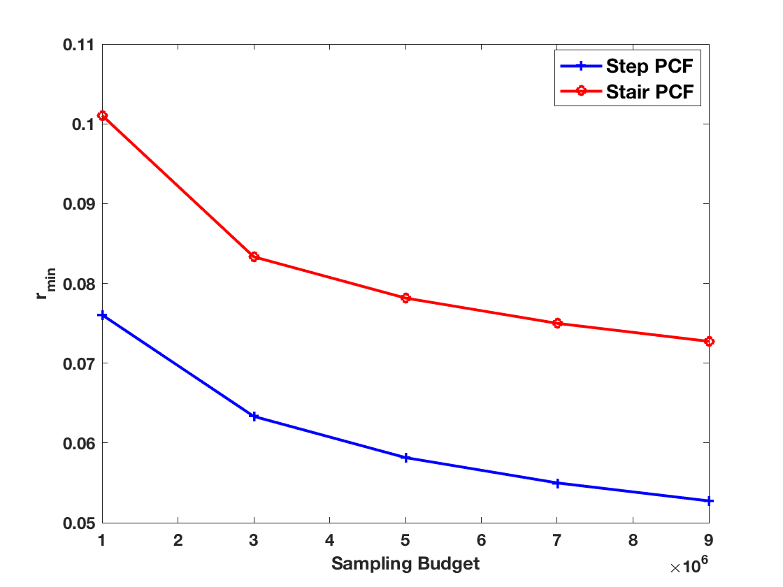
In this section, we show the increase in coverage (or $r_{min}$) obtained by compromising randomness by increasing peak height in the PCF. We constrain the peak height to be below $P_{0}\leq 1.5$ and analyze the gain in $r_{min}$ due to this small compromise in randomness. Furthermore, we assume that $r_{min}^{step}\leq r_{0}\leq 2\times r_{min}^{step}$ and $r_{0}\leq r_{1}\leq 1.5\times r_{0}$. In Figures 7(a) through 7(e), we compare the maximum $r_{min}$ achieved by the Step and Stair PCF designs, for varying sample sizes in dimensions $2$ to $6$. It can be seen that introducing a small peak in the PCF results in a significant increase in the coverage. This gain can be observed for all sampling budgets in all dimensions. Furthermore, as expected, for low sampling budgets maximal gain is observed, and should decrease with increasing $N$ as the $r_{min}$ for both the families will asymptotically (in $N$) converge to zero.

7.2.2 Relative Radius $\rho$ vs. Dimension $d$

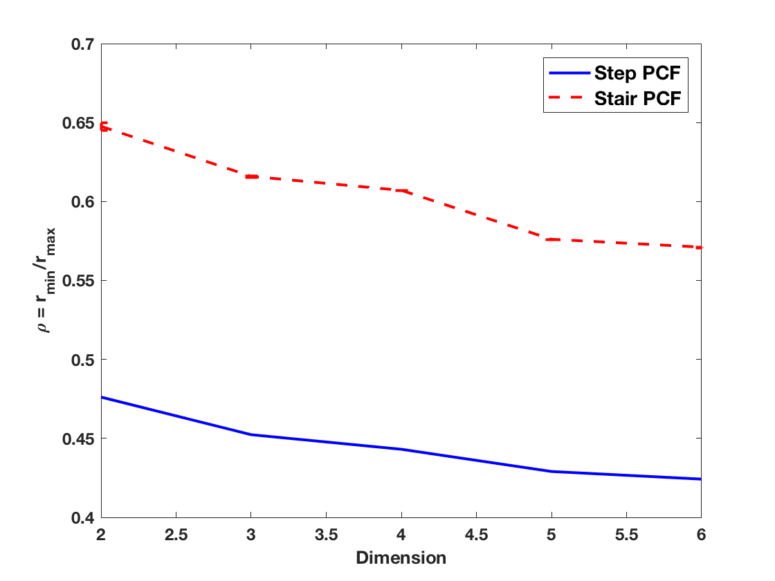
In this section, we study the increase in relative radius $\rho$ due to the introduction of a peak in the PCF. Again, we assume that $P_{0}\leq 1.5$, $r_{min}^{step}\leq r_{0}\leq 2\times r_{min}^{step}$ and $r_{0}\leq r_{1}\leq 1.5\times r_{0}$. In Figure 8, we show the maximum $\rho=r_{min}/r_{max}$ achieved by the Step and Stair PCFs for different dimensions $d$. For Stair PCF, we do not have a closed form expression of $\rho$, thus, we obtain the maximum achievable $r_{min}$ empirically for various sampling budgets and plot the mean (with standard deviation) behavior of the $\rho$. It can be seen that introducing a small peak in the PCF results in a significant increase in the relative radius. This gain can be observed at all sampling budgets in all dimensions. This also corroborates the recommendation of using $0.65\leq\rho\leq 0.85$ in practice for coverage based designs and suggests that in higher dimensions $\rho$ should be higher.

Figure 8: (a) Gain in the relative radius $\rho$ achieved with the Stair PCF constructions, in comparison to the Step PCF constructions; (b) Upper bound on the reconstruction error of Step and Stair PCF based constructions.

7.2.3 Analysis of Reconstruction Error Upper Bound

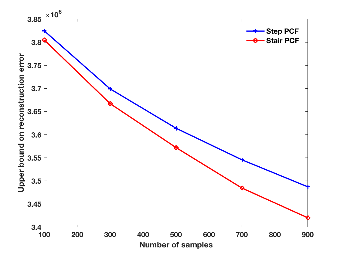
We also assess the reconstruction quality of the Step and Stair PCF based spectral designs, on the class of periodic functions considered in Section 5.1, for varying sampling budgets. Here, we consider the setup where $0\leq k\leq 1000$ and $0\leq f\leq 1000$. In Figure 8, we plot the average reconstruction error upper bounds as given in (11) for Step and Stair PCF. As expected, for both sample designs, the reconstruction error decreases with an increase in the sampling budget. More interestingly, the reconstruction error of Stair PCF is lower compared to the reconstruction error of Step PCF, thus showing the effectiveness of increased coverage in sample designs.

8 Synthesis of Space-filling Spectral Designs

In this section, we describe the proposed approach for synthesizing sample designs that match the optimal (Stair or Step) PCF characteristics. Existing approaches for PCF matching such as (Öztireli and Gross, 2012; Kailkhura et al., 2016b) rely on kernel density estimators to evaluate the PCF of a point set. A practical limitation of these approaches is the lack of an efficient PCF estimator in high dimensions. More specifically, these estimators are biased due to lack of an appropriate edge correction strategy. This bias in PCF estimation arises due to the fact that sample hyper-spheres used in calculating point-pattern statistics may fall partially outside the study region and will produce a biased estimate of the PCF unless a correction is applied. The effect of this bias is barely noticeable in $2$ dimensions and hence existing PCF matching algorithms have ignored this. However, this problem becomes severe in higher dimensions, thus, making the matching algorithm highly inaccurate. To address this crucial limitation, we introduce an edge corrected estimator for computing the PCF of sample designs in arbitrary dimensions. Following this, we describe a gradient descent based optimization technique to synthesize samples that match the desired PCF.

8.1 PCF Estimation in High Dimensions with Edge Correction

In order to create an unbiased PCF estimator, we propose to employ an edge corrected kernel density estimator, defined as follows:

$$\hat{G}(r)=\frac{V_{W}}{\gamma_{W}}\frac{V_{W}}{N}\frac{1}{S_{E}(N-1)}\sum\limits_{i=1}^{N}\underset{i\neq j}{\sum\limits_{j=1}^{N}}k\left(r-|x_{i}-x_{j}|\right)$$ (24)

where $k(.)$ denotes the kernel function; here we use the classical Gaussian kernel

$$k(z)=\frac{1}{\sqrt{\pi}\sigma}\exp\left(-\frac{z^{2}}{2\sigma^{2}}\right).$$ (25)

In the above expression, $V_{W}$ indicates the volume of the sampling region. When the sampling region is a hyper-cube with length $1$, we have $V_{W}=1$. Let $S_{E}$ denote the area of hyper-sphere with radius $r$ which is given by

$$S_{E}=\dfrac{dr^{d-1}\pi^{\frac{d}{2}}}{\Gamma(1+\frac{d}{2})}.$$

Also, we denote the surface area of the sampling region by $S_{W}$, which is expressed as

$$S_{W}=r^{d-1}\sin^{d-2}\phi_{1}\sin^{d-3}\phi_{2}\cdots\sin\phi_{d-2}.$$

The term $\frac{V_{W}}{\gamma_{W}}$ performs edge correction to handle the unboundedness of the estimator, where $\gamma_{W}$ is an isotropic set covariance function given by

$$\gamma_{W}=\dfrac{1}{S_{E}}\underset{\underset{0\leq\phi_{i}\leq\pi,i=1\;\text{to}\;d-2}{0\leq\phi_{d-1}\leq 2\pi}}{\int}S_{W}\gamma d\phi_{1}\cdots d\phi_{d-1}$$ (26)

where $\gamma=\prod_{p=1}^{d}(1-|x^{p}|)$ with

$$x^{1}=r\cos\phi_{1}$$

$$x^{2}=r\sin\phi_{1}\cos\phi_{2}$$

$$x^{3}=r\sin\phi_{1}\sin\phi_{2}\cos\phi_{3}$$

$$\vdots$$

$$x^{d-1}=r\sin\phi_{1}\cdots\sin\phi_{d-2}\cos\phi_{d-1}$$

$$x^{d}=r\sin\phi_{1}\cdots\sin\phi_{d-2}\sin\phi_{d-1}.$$

(a) $d=2$

(b) $d=3$

(c) $d=4$

(d) $d=5$

(e) $d=6$

Figure 9: (a) Incorrect PCF estimation due to the use of an approximate edge correction factor, (b)-(f) Effectiveness of the approximation edge correction, obtained using polynomial regression, in comparison to the true edge correction from the evaluation of a multi-dimensional integral, for dimensions $2$ to $6$.

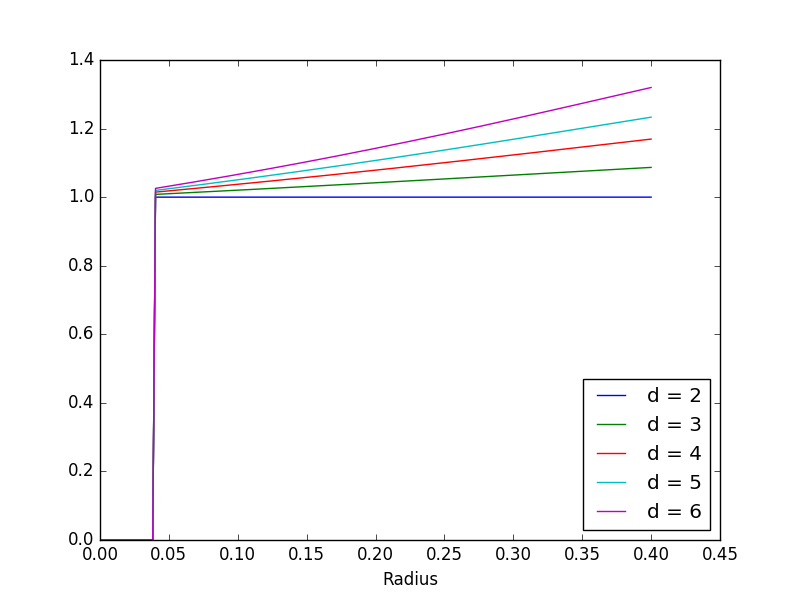
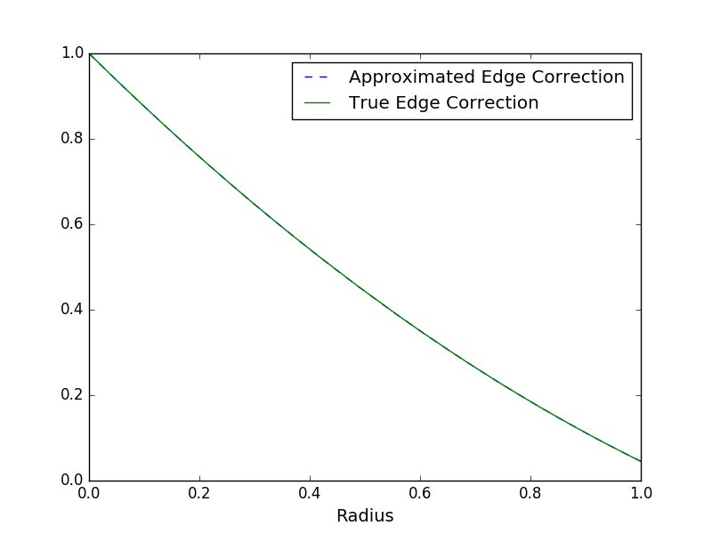
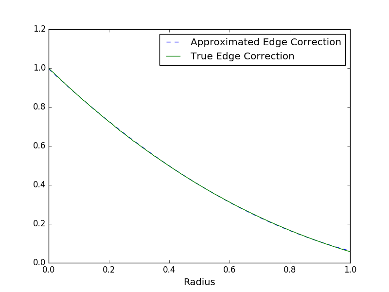
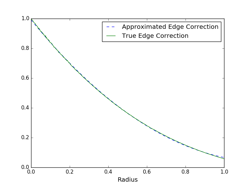
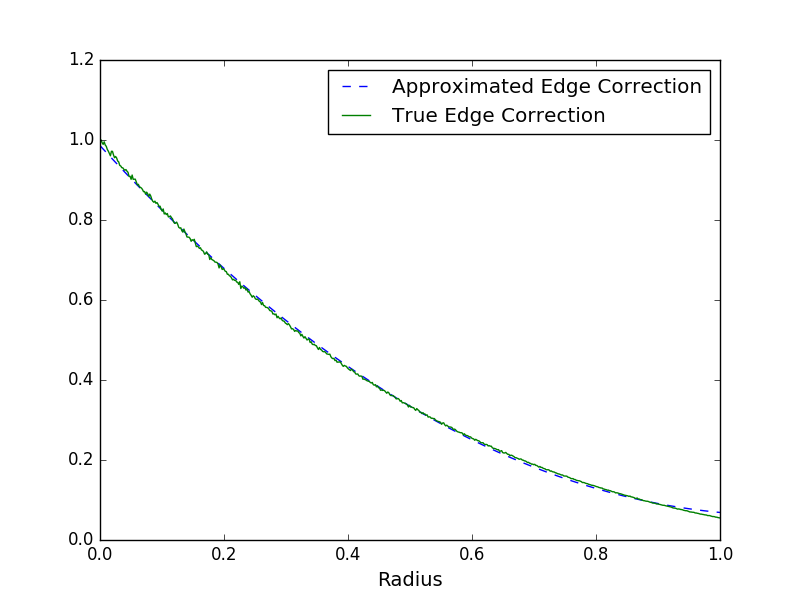
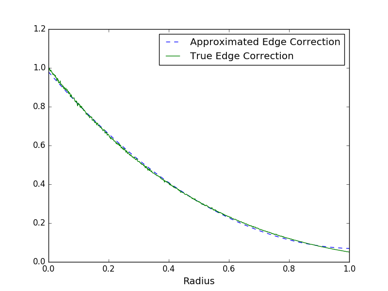
In Figure 9, we show that by using an approximate edge correction factor (using the same factor as $d=2$), the PCF is wrongly estimated. Moreover, as the dimension increases, the estimated PCF moves farther away from the true PCF very quickly.

Note that, the calculation of the correct edge correction factor requires the evaluation of a multi-dimensional integral which is computationally expensive in high dimensions. In this paper, we provide a closed form approximation of $\gamma_{W}$ (using polynomial regression of order $2$) in different dimensions $d=2$ to $6$ when $r\leq 1.0$. More specifically, we have the following approximation $\hat{\gamma_{W}}=1-a_{1}r+a_{2}r^{2}$ where $a_{1}$ and $a_{2}$ are as given below.

Dimension	$d=2$	$d=3$	$d=4$	$d=5$	$d=6$
$a_{1}$	$4/\pi$	$1.47$	$1.63$	$1.75$	$1.89$
$a_{2}$	$1/\pi$	$0.54$	$0.72$	$0.87$	$1.04$

It can be observed from Figures 9(a) through 9(e) that the proposed approximations are quite tight.

8.2 Synthesis Algorithm

The underlying idea of the proposed algorithm is to iteratively transform an initial random input sample design such that its PCF matches the target PCF. In particular, we propose a non-linear least squares formulation to optimize for the desired space-filling properties. Let us denote the target PCF by $G^{*}(r)$. We discretize the radius $r$ into $m$ points $\{r_{j}\}_{j=1}^{m}$ and minimize the sum of the weighted squares of errors between the target PCF $G^{*}(r_{j})$ and the curve-fit function (kernel density estimator of PCF) $G(r_{j})$ over $m$ points. This scalar-valued goodness-of-fit measure is referred to as the chi-squared error criterion and can be posed as a non-linear weighted least squares problem as follows.

$$\arg\min\;\;\sum\limits_{j=1}^{M}\left(\dfrac{G(r_{j})-G^{*}(r_{j})}{w_{j}}\right)^{2},$$

where $w_{j}$ indicates the weight (importance) assigned to the fitting error at radius $r_{j}$. This optimization problem can be efficiently solved using a variant of gradient descent algorithm (discussed next), that in our experience converges quickly. In the simplest cases of uniform weights the solution tends to produce a higher fitting error at lower radii $r_{j}$. To address this challenge we use a non-uniform distribution for the weights $\{w_{j}\}$. These weights are initialized to be uniform and are updated in an adaptive fashion in the gradient descent iterations. The weight $w_{j}$ at gradient descent iteration $t+1$ is given by (Kailkhura et al., 2016b):

$$w_{j}=\dfrac{1}{|G^{t}(r_{j})-G^{*}(r_{j})|}$$

where $G^{t}(r_{j})$ is the value of the PCF at radius $r_{j}$ during the gradient descent iteration $t$. Note that, PCF matching is a highly non-convex problem. We found that the following trick further helps solve PCF matching problem more efficiently.

8.2.1 One Sided PCF Smoothing

We propose to perform one sided smoothing of the target PCF which is given as follows:

$$\hat{G}^{*}(r)=\left\{\begin{array}[]{rll}(cr)^{b}&\mbox{if}\ r<r_{\text{min}}\\ 1&\mbox{if}\ r\geq r_{\text{min}}.\end{array}\right.$$

where $c$ is some pre-specified constant and $b>1$ is the smoothing constant obtained via cross-validation. More specifically, we add polynomial noise in the low radius region of the PCF. This can also be interpreted as polynomial approximation of the PCF in the low radii regime. We have noticed that sometimes adding a controlled amount of Gaussian noise instead of polynomial noise also improves the performance.

8.2.2 Edge Corrected Gradient Descent

The non-linear least squares problem is solved iteratively using gradient descent. Starting with a random point set $X=\{x_{i}\}_{i=1}^{N}$, we iteratively update $x_{i}$ in the negative gradient direction of the objective function. At each iteration $k$, this can be formally stated as

$$x_{i}^{k+1}=x_{i}^{k}-\lambda\dfrac{\Delta_{i}}{|\Delta_{i}|},$$

where $\lambda$ is the step size and $\Delta_{i}=\{\Delta_{i}^{k}\}_{k=1}^{d}$ in the normalized edge corrected gradient is given by

$$\Delta_{i}^{p}=\underset{i\neq l}{\sum} \dfrac{(x_{l}^{p}-x_{i}^{p})}{|x_{l}-x_{i}|}\sum_{j=1}^{m}\dfrac{G(r_{j})^{k}-G^{*}(r_{j})}{w_{j}(1-a_{1}r_{j}+a_{2}r_{j}^{2})r_{j}^{d-1}}$$

$$\left(|x_{l}-x_{i}|-r_{j}\right)k\left(r_{j}-|x_{i}-x_{l}|\right).$$ (27)

We re-evaluate the PCF $G(r_{j})^{k}$ of the updated point set after each iteration using the unbiased estimator from the previous section.

Figure 10: Step PCF synthesis using one sided PCF smoothing technique. 10 $d=2$ 10 $d=3$ 10 $d=4$ 10 $d=5$ 10 $d=6$.

Figure 11: Stair PCF synthesis using one sided PCF smoothing technique. 11 $d=2$ 11 $d=3$ 11 $d=4$ 11 $d=5$ 11 $d=6$.

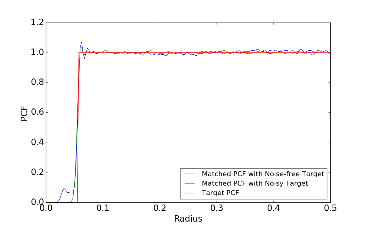
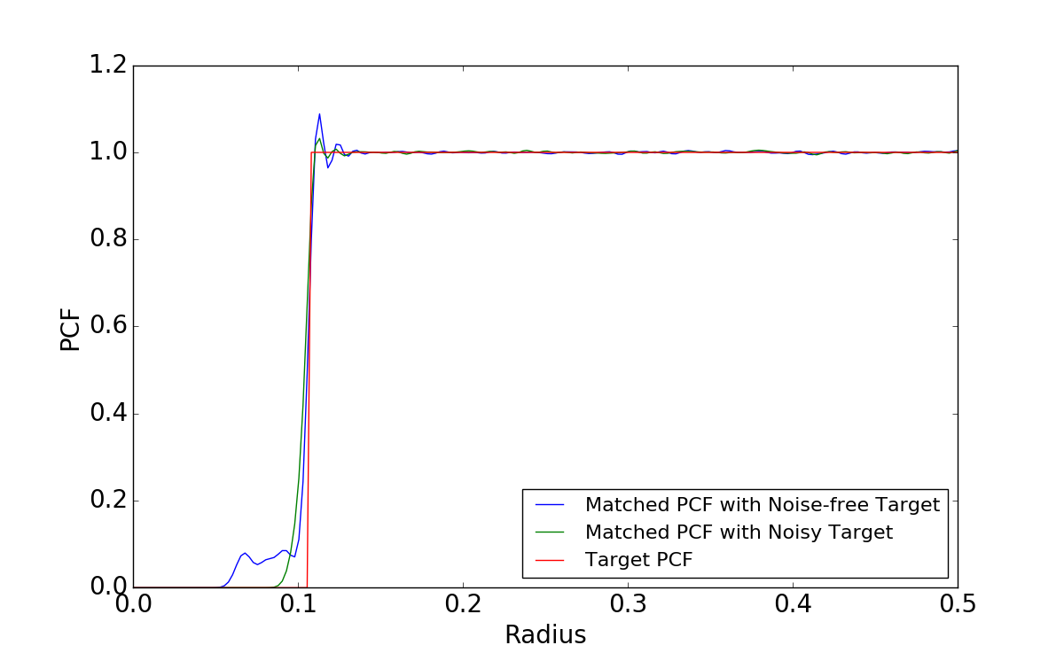
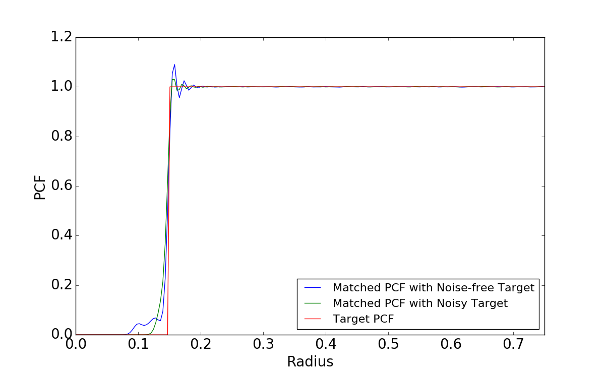
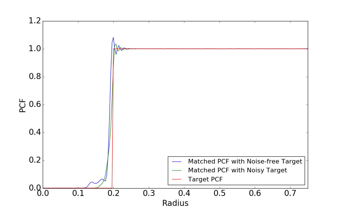
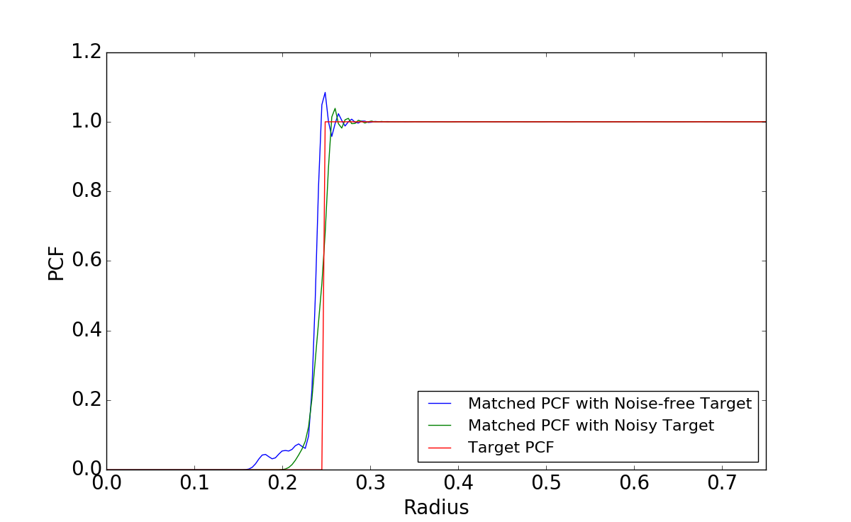
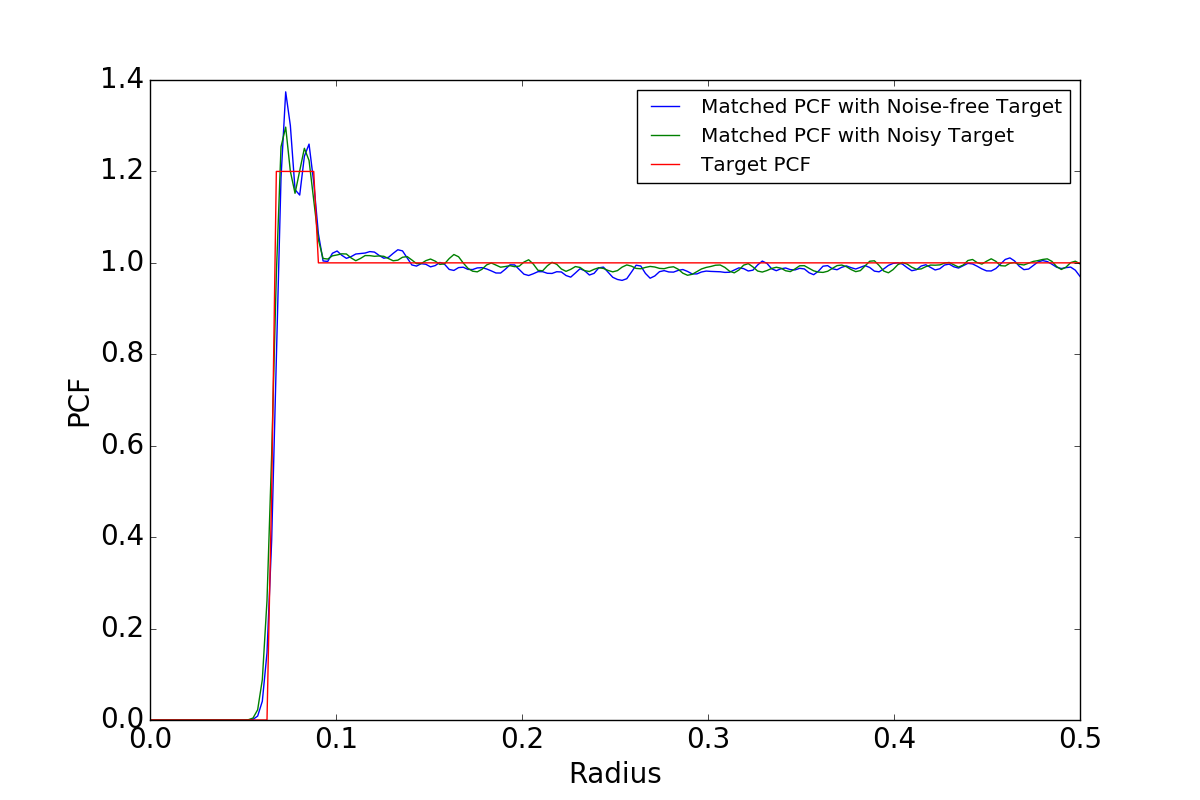
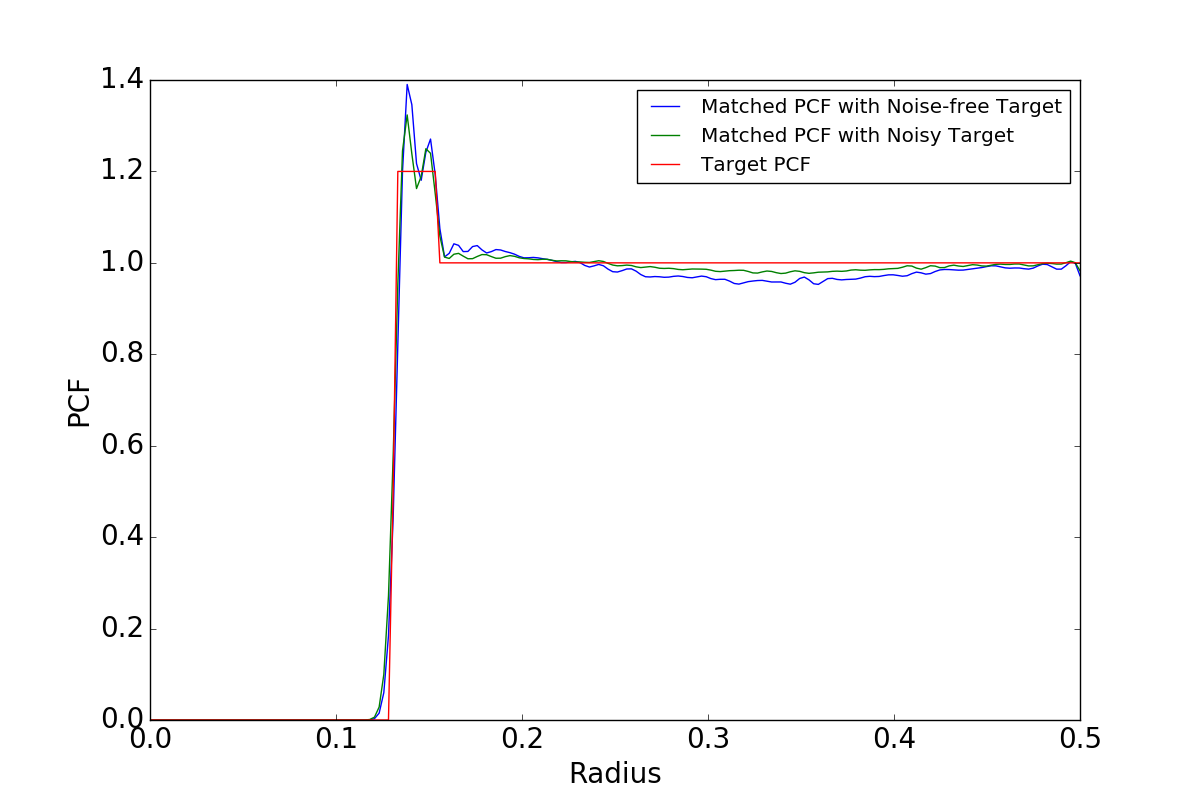
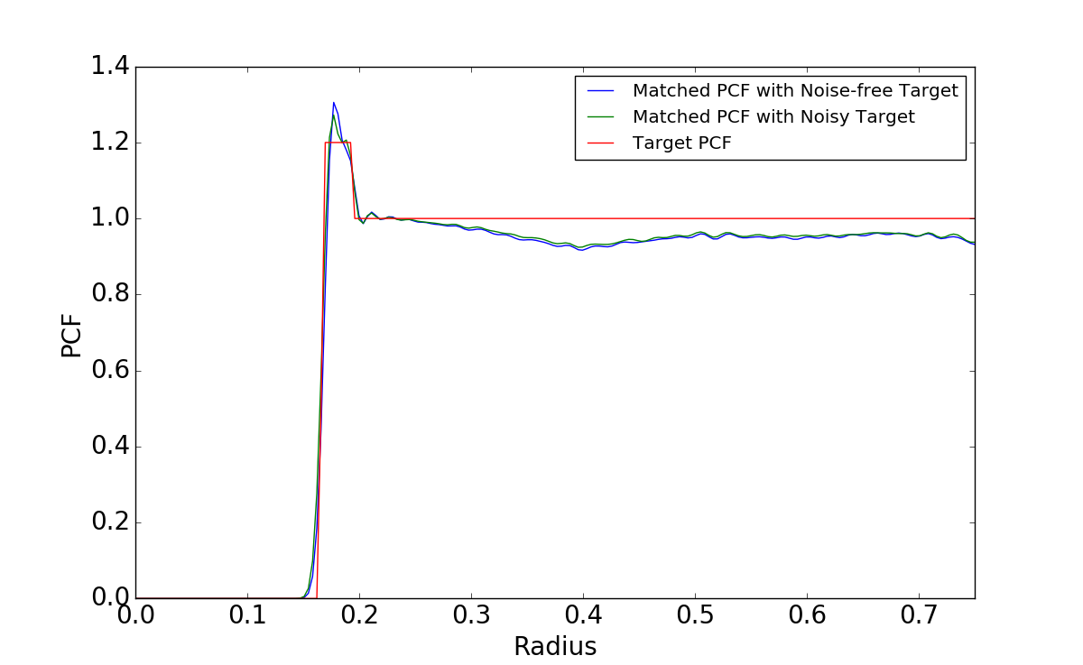
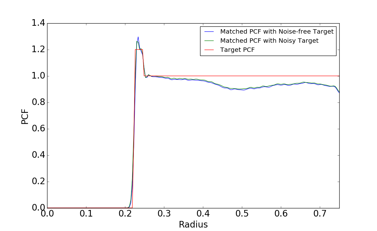
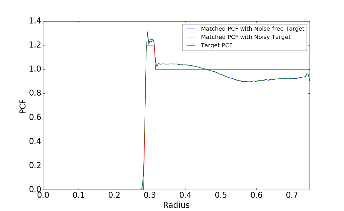
In Figure 10, we compare the behavior of the proposed PCF matching algorithm with and without the one sided PCF smoothing. The target PCF is designed using a Step PCF design with $r_{min}$ as given in Proposition 10. PCF matching is carried out with varying sampling budget, $N=100,\;200,\;400,\;600,\;800$ for $d=2,\;3,\;4,\;5,\;6$, respectively. The variances of the Gaussian kernel were set at $\sigma^{2}=0.0065,\;0.007,\;0.01,\;0.01,\;0.01$ for $d=2,\;3,\;4,\;5,\;6$, respectively and the step size for the gradient descent algorithm was fixed at $0.001$. The value of $b$ was obtained using cross-validation. The initial point set was generated randomly (uniform) in the unit hyper-cube and matching was carried for $100$ gradient descent iterations. It can be observed that the proposed algorithm produces an accurate fit to the target, and that the smoothing actually leads to improved performance.

In Figure 11, we demonstrate the synthesis of a Stair PCF based spectral design, using parameters $P_{0}=1.2,\delta=0.025$. Similar to the previous case, PCF matching is carried out with varying sampling budget, $N=100,\;200,\;400,\;600,\;800$, for $d=2,\;3,\;4,\;5,\;6$ respectively. The variances of the Gaussian kernel were set at $\sigma^{2}=0.0065,\;0.007,\;0.01,\;0.01,\;0.01$ for $d=2,\;3,\;4,\;5,\;6$, respectively and the step size for the gradient descent algorithm was fixed at $0.001$. We found that matching the Stair PCF is more challenging for a gradient descent optimization compared to the Step PCF. When a random point set is used for initialization, reaching convergence takes much longer. However, choosing the initial point set intelligently improves the quality of matching significantly. In all our experiments, we used the maximal PDS (Ebeida et al., 2012) to initialize the optimization and matching was carried for $100$ gradient descent iterations. We observed that another reasonable choice for the initialization is a regular grid sample, and interestingly in most cases it matches the performance of the MPDS initialization. Furthermore, one sided PCF smoothing does not provide significant improvements in this case, particularly in higher dimensions.

9 Experiments

In this section, we evaluate the qualitative performance of proposed space-filling spectral designs and present comparisons to popularly adopted space-filling designs, such as LHS, QMC and MPDS. Note that, currently, there does not exist any PDS synthesis approach which can generate sample sets with a desired size $N$ while achieving user-specified spatial characteristics (e.g. relative radius). In all PDS synthesis approaches, there is no control over the number of samples generated by the algorithm which makes the use of these algorithms difficult in practice. However, the proposed approach can control both $N$ and $r_{min}$ simultaneously. For our qualitative comparison, we perform three empirical studies, in dimensions $2$ to $6$ : (a) image reconstruction, (b) regression on several benchmark optimization functions, and (c) surrogate modeling for an inertial confinement fusion (ICF) simulation code.

Table 1: Impact of different space-filling designs on image reconstruction performance. In all cases, we show the reconstructed images and their PSNR values.

$\boldsymbol{\alpha}$	Sobol	Halton	LHS	MPDS	Step	Stair
0.001
	14.82 dB	15.75 dB	14.29 dB	16.90 dB	16.00 dB	16.46 dB
0.002
	12.10 dB	12.34 dB	11.39 dB	13.16 dB	12.58 dB	12.96 dB
0.003
	11.22 dB	11.38 dB	10.75 dB	11.88 dB	11.55 dB	11.78 dB
0.004
	10.61 dB	10.67 dB	10.34 dB	10.92 dB	10.80 dB	10.90 dB
0.005
	9.80 dB	9.70 dB	9.59 dB	9.82 dB	9.83 dB	9.84 dB
0.006
	9.09 dB	8.97 dB	8.97 dB	8.96 dB	9.08 dB	9.02 dB
0.007
	8.49 dB	8.39 dB	8.51 dB	8.32 dB	8.49 dB	8.42 dB

9.1 Image Reconstruction

In this experiment, we consider the problem of designing sample distributions for image reconstruction. More specifically, we consider the commonly used zone plate test function:

$$z(r)=(1+\cos(\alpha r^{2}))/2,$$

with varying levels of complexity (or frequency content) $\alpha$. Note that, we choose the zone plate for our study over natural images, since it shows the response for a wide range of frequencies and aliasing effects that are not masked by image features. For all zone plate renderings in this paper, we have tiled toroidal sets of $1000$ $2$-dimensional points over the image-plane and utilized a Lanczos filter with a support of width $4$ for resampling. Further, we also report the peak signal-to-noise ratio (PSNR) as a quantitative error measure:

$$\text{PSNR}=20\log_{10}\dfrac{1}{\text{MSE}},$$

where MSE is the mean squared error. However, it is well known in the image processing community that PSNR can be a weak surrogate for visual quality and, therefore, we also show the reconstructed images.

Table 1 illustrates the reconstructions obtained using different space-filling designs, for varying values of $\alpha$. It can be observed from the results that the QMC sequences produce a large amount of aliasing artifacts in the high frequency regions, which can be directly linked to the oscillations in their corresponding PCFs. On the other hand, LHS design recovers a small amount of low-frequencies, and maps most of the frequencies to white noise due to its small $r_{min}$ and near-constant PCF. In contrast, sample designs which attempt to trade-off between coverage and randomness properties, i.e., MPDS and the proposed spectral space-filling designs (as seen in Figure 3), have superior reconstruction quality. These designs reduce the aliasing artifacts, have cleaner low frequency content (upper left corner)) and map all high frequencies (bottom right corner) to white noise. More interestingly, we see that for low complexity cases, i.e., lower $\alpha$, the MPDS performs the best followed by the proposed Stair and Step PDS respectively. For moderately complex images, the Stair PDS performs the best followed by the Step and the MPDS. Finally, for highly complex images, the Step PDS performs the best followed by the Stair and the MPDS. These observations corroborate our discussion in Section 5.2 that an increase in $r_{min}$ (coverage) in the PCF results in an increase in the range of low frequencies that can be recovered without aliasing, and equivalently reduction in the amount of oscillations (or an increase in randomness) in the PCF leads to reduced oscillations in the PSD, which in turn indicates a systematic mapping of high frequency content to white noise.

9.2 Regression Modeling for Benchmark Optimization Functions

In this study, we consider the problem of fitting regression models to analytical functions and perform a comparative study of different sample designs, in terms of their generalization performance. More specifically, we consider a set of benchmark analytic functions between dimensions $2$ and $6$, that are commonly used in global optimization tests (Jamil and Yang, 2013). They are chosen due to their diversity in terms of their complexity and shapes. We compare the performance of proposed space-filling spectral designs (Step, Stair) with coverage based designs (MPDS), low-discrepancy designs (Halton and Sobol), latin hypercube sampling and random sampling. Appendix A lists the set of functions used in our experiments. In each case, we fit a random forest regressor with $30$ trees and repeated for $20$ independent realizations of sample designs. We evaluate the generalization performance on $10^{6}$ regular grid based test samples. Finally, we employ $3$ popular quality metrics to quantify the performance of the resulting regression models: mean squared error (MSE), relative average absolute error (AAE), and the R²-statistic. The metrics are defined as follows:

$$MSE(\mathbf{y},\hat{\mathbf{y}})=\frac{\sum_{i=1}^{N}(y_{i}-\hat{y}_{i})^{2}}{N},$$ (28)

$$AAE(\mathbf{y},\hat{\mathbf{y}})=\frac{\sum_{i=1}^{N}|y_{i}-\hat{y}_{i}|}{N*STD(\mathbf{y})},$$ (29)

$$R^{2}(\mathbf{y},\hat{\mathbf{y}})=1-\frac{\sum_{i=1}^{N}(y_{i}-\hat{y}_{i})^{2}}{\sum_{i=1}^{N}(y_{i}-MEAN(\mathbf{y}))^{2}}$$ (30)

where $\mathbf{y}=f(\mathbf{x})$ are the true function values and $\hat{\mathbf{y}}$ are the predicted values.

Tables 2 through 6 show the performance of different space-filling designs for various analytic functions in dimensions $2$ to $6$, respectively. We see that, for $d=2$ (Table 2), LHS and Halton sequences perform better compared to the rest of the sample designs on most of the test functions. However, on some functions, e.g., GoldsteinPrice, Stair PCF and MPDS perform better. Therefore, none of the sample designs consistently guarantee superior performance. For $d=3$ (Table 3), we see that Stair PCF design and MPDS (followed by Sobol sequences) perform consistently better compared to the rest of the approaches. As we go higher in dimensions, i.e., $d>3$, we notice a significant gain in the performance of Stair PCF based space-filling spectral designs. Interesting, the amount of performance gain of Stair PCF based design increases as we go higher in dimensions. The reason for the poor performance of QMC sequences and LHS for $d>3$ is due to their poor space-filling properties in high dimensions (Wang and Sloan, 2008). In comparison, both space-filling spectral designs and MPDS have good space-filling properties. We found that Stair PCF design and MPDS have similar coverage characteristics ($r_{min}$). However, the difference in their performance can be attributed to the fact that MPDS designs have significantly more oscillations in their PCF compared to an equivalent Stair PCF based space-filling spectral design, i.e. violation of the randomness objective.

Table 2: Impact of sample design on generalization performance of regression models fit to benchmark analytical functions in $2$ dimensions. LHS and Halton sequences perform slightly better compared to rest of the sample designs.

Function	MSE	AAE	R2-Statistic
GoldsteinPrice
Chichinadze
Rosenbrock
Cube

Table 3: Impact of sample design on generalization performance of regression models fit to benchmark analytical functions in $3$ dimensions. While the Stair PCF and MPDS designs are consistently better than the other methods, the amount of performance gain is minimal.

Function	MSE	AAE	R2-Statistic
BoxBetts
Hartmann3
Wolfe
Helical Valley

Table 4: Impact of sample design on generalization performance of regression models fit to benchmark analytical functions in $4$ dimensions. Stair PCF and MPDS designs demonstrate appreciable gains over popular sample design choices.

Function	MSE	AAE	R2-Statistic
DeVilliersGlasser01
Colville
Powell

Table 5: Impact of sample design on generalization performance of regression models fit to benchmark analytical functions in $5$ dimensions. In higher dimensions, conventional methods such as the LHS and QMC perform very poorly, while Stair PCF design significantly outperforms all competing methods, because of improved trade-off between coverage and randomness properties.

Function	MSE	AAE	R2-Statistic
Dolan
BiggsExp05

Table 6: Impact of sample design on generalization performance of regression models fit to benchmark analytical functions in $6$ dimensions. Even with highly complex functions such as the Hartmann6, the proposed Stair PCF based spectral space-filling design produces more accurate regression models, thus evidencing the importance of improved space-filling characteristics.

Function	MSE	AAE	R2-Statistic
Trid
Hartmann6

Table 7: Performance of surrogate models for the NIF $1-$d HYDRA simulator using different sample design techniques, with varying number of input parameters. While the conventional sample designs achieve reasonable performance in low dimensions, the proposed Stair PCF based design is consistently superior as the dimension of the input space grows.

Function	MSE	AAE	R2-Statistic
Parameter Space Dimension = 2
PEAK fusion power
Parameter Space Dimension = 3
Radiation energy
Parameter Space Dimension = 4
MINradius shock
Parameter Space Dimension = 5
MINradius shock
Parameter Space Dimension = 6
MAXpressure

9.3 Surrogate Model Design for an Inertial Confinement Fusion (ICF) Simulator

In this subsection, we consider the problem of designing surrogate models for an inertial confinement fusion (ICF) simulator developed at the National Ignition Facility (NIF). The NIF is aimed at demonstrating inertial confinement fusion (ICF), that is, thermonuclear ignition and energy gain in a laboratory setting. The goal is to focus $192$ beams of the most energetic laser built so far onto a tiny capsule containing frozen deuterium. Under the right conditions, the resulting pressure will collapse the target to the point of ignition where hydrogen starts to fuse and produce massive amounts of energy, effectively creating a small star which can be harnessed for energy production. Though significant progress has been made, the ultimate goal of “ignition” has not yet been reached.

NIF employs an adaptive pipeline: perform experiments, use post-shot simulations to understand the experimental results, and design new experiments with parameter settings that are expected to improve performance. From an analysis viewpoint, the goal is to search the parameter space to find the region that leads to near-optimal performance. The dataset considered here is a so called engineering or macro-physics simulation ensemble in which an implosion is simulated using different input parameters, such as, laser power, pulse shape etc. From these simulations, scientists extract a set of drivers, physical quantities believed to determine the behavior of the resulting implosion. These drivers are then analyzed with respect to the energy yield to better understand how to optimize future experiments. As one can expect, the success of this pipeline heavily depends on the quality of samples used for post-shot simulations.

We use the NIF $1$-d HYDRA simulator (Marinak et al., 2001) and compare the performance of proposed space-filling spectral designs with existing approaches (random, LHS, Halton and Sobol and MPDS). For each simulation run, a large number of output quantities, such as peak velocity, yield, etc., are computed, and subsequently used to describe the resulting implosion. We vary the number of input parameters between $2$ and $6$, and fix the remaining variables to their default values. In each case, we fit a random forest regressor with $30$ trees and repeated for $20$ independent realizations of sample designs. We evaluated the reconstruction performance on $10^{5}$ regular grid based test samples using the metrics in the previous experiment.

Table 7 shows the regression performance of the different sample designs for various output quantities in dimensions $2$ to $6$. We observe that regression error patterns are consistent with our observations in Section 9.2. The proposed Stair PCF based design consistently performs the best (followed by MPDS) for $d\geq 3$. Furthermore, the performance gain with the Stair PCF based design improves as we go higher in dimensions. This performance gain can be credited to their ability to achieve better space-filling properties in high dimensions by intelligently balancing the trade-off between coverage and randomness, and the effectiveness of the quality metric (PCF) adopted for design and optimization.

10 Conclusion and Future Directions

In this work, we considered the problem of constructing high quality space-filling designs. We proposed the use of pair correlation function (PCF) to quantify the space-filling property and systematically traded-off coverage and randomness in sample designs in arbitrary dimensions. Next, we linked PCF to the power spectral density (PSD) to analyze the objective measure of the design performance. Using the insights provided by this spatial-spectral analysis, we proposed novel space-filling spectral designs. We also provided an efficient PCF estimator to evaluate the space-filling properties of sample designs in arbitrary dimensions. Next, we devised a gradient descent based optimization algorithm to generate high quality space-filling designs. Superiority of proposed space-filling spectral designs were shown on two different applications in $2$ to $6$ dimensions: a) image reconstruction and b) surrogate modeling on several benchmark optimization functions and an inertial confinement fusion (ICF) simulation code. There are still many interesting questions that remain to be explored in the future work such as an analysis of the problem for non-linear manifolds. Note that, some analytical methodologies used in this paper are certainly exploitable for studying and designing space-filling designs in different manifolds. Other questions such as PCF parameterizations for other variants of space-filling designs and optimization approaches to synthesize them can also be investigated.

Acknowledgments

Acknowledgments This work was performed under the auspices of the U.S. Department of Energy by Lawrence Livermore National Laboratory under Contract DE-AC52-07NA27344. LLNL-JRNL-743060

A Benchmark Optimization Functions

A.1 2 Dimensional Functions

Rosenbrock: $\sum_{p=1}^{2}\left(100((x^{p})^{2}-x^{p+1})+(x^{p}-1)^{2}\right)$
Cube: $100(x^{2}-(x^{1})^{3})^{2}+(1-x^{1})^{2}$
Chichinadze: $(x^{1})^{2}-12x^{1}+8\sin(2.5\pi x^{1})+10\cos(0.5\pi x^{1})+11-0.2\dfrac{\sqrt{5}}{\exp(0.5(x^{2}-0.5)^{2})}$
GoldsteinPrice: $\left(1+(x^{1}+x^{2}+1)^{2}(19-14x^{1}+3(x^{1})^{2}-14x^{2}+6x^{1}x^{2}+3(x^{2})^{2})\right)\\ \qquad\left(30+(2x^{1}-3x^{2})^{2}(18-32x^{1}+12(x^{1})^{2}+48x^{2}-36x^{1}x^{2}+27(x^{2})^{2})\right)$

A.2 3 Dimensional Functions

BoxBetts: $\sum_{p=1}^{3}g(x^{i})^{2};g(x)=\exp(-0.1(p+1)x^{1})-\exp(-0.1(p+1)x^{2})-(\exp(-0.1(p+1))-\exp(-(p+1))x^{3})$
HelicalValley: $100(x^{3}-10\psi(x^{1},x^{2}))^{2}+(\sqrt{(x^{1})^{2}+(x^{2})^{2}}-1)^{2}+(x^{3})^{2};2\pi\psi(x^{1},x^{2})=\tan^{-1}(x^{2}/x^{1})\;\textbf{if}\;x^{1}\geq 0,\;\textbf{and}\;\pi+\tan^{-1}(x^{2}/x^{1})\;\textbf{otherwise.}$
Wolfe: $\frac{4}{3}((x^{1})^{2}+(x^{2})^{2}-x^{1}x^{2})^{0.75}+x^{3}$
Hartmann3: $-\sum_{i=1}^{4}c_{i}\exp(-\sum_{j=1}^{3}a_{ij}(x^{j}-p_{ij})^{2})$

A.3 4 Dimensional Functions

DeVilliersGlasser01: $\sum_{i=1}^{24}\left(x^{1}(x^{2})^{0.1(i-1)}\sin(x^{3}(0.1(i-1))+x^{4})-y_{i}\right)^{2}$
Powell: $(x^{3}+10x^{1})^{2}+5(x^{2}-x^{4})^{2}+(x^{1}-2x^{2})^{4}+10(x^{3}-x^{4})^{4}$
Colville: $(x^{1}-1)^{2}+100((x^{1})^{2}-x^{2})^{2}+10.1(x^{2}-1)^{2}+(x^{3}-1)^{2}+90((x^{3})^{2}-x^{4})^{2}+10.1(x^{4}-1)^{2}+19.8\frac{x^{4}-1}{x^{2}}$

A.4 5 Dimensional Functions

BiggsExp05: $\sum_{i=1}^{11}(x^{3}e^{-t_{i}x^{1}}-x^{4}e^{-t_{i}x^{2}}+3e^{-t_{i}x^{5}}-y_{i})^{2};\;t_{i}=0.1i;\;y_{i}=e^{-t_{i}}-5e^{-10t_{i}}+3e^{-4t_{i}}$
Dolan: $|(x61+1.7x^{2})\sin(x^{1})-1.5x^{3}-0.1x^{4}\cos(x^{5}-x^{1})+0.2(x^{5})^{2}-x^{2}-1|$

A.5 6 Dimensional Functions

Trid: $\sum_{p=1}^{6}(x^{p}-1)^{2}-\sum_{p=2}^{6}x^{p}x^{p-1}$
Hartmann6: $-\sum_{i=1}^{4}c_{i}\exp(-\sum_{j=1}^{6}a_{ij}(x^{j}-p_{ij})^{2})$

References

- Anirudh et al. (2017) R. Anirudh, B. Kailkhura, J. J. Thiagarajan, and P. T. Bremer. Poisson disk sampling on the grassmannnian: Applications in subspace optimization. In 2017 IEEE Conference on Computer Vision and Pattern Recognition Workshops (CVPRW), pages 690–698, July 2017. doi: 10.1109/CVPRW.2017.98.
- Balzer et al. (2009) Michael Balzer, Thomas Schlömer, and Oliver Deussen. Capacity-constrained point distributions: A variant of lloyd’s method. ACM Trans. Graph., 28(3):86:1–86:8, July 2009. ISSN 0730-0301. doi: 10.1145/1531326.1531392.
- Bridson (2007) Robert Bridson. Fast poisson disk sampling in arbitrary dimensions. In ACM SIGGRAPH 2007 Sketches, SIGGRAPH ’07, New York, NY, USA, 2007. ACM. doi: 10.1145/1278780.1278807.
- Caflisch (1998) Russel E. Caflisch. Monte carlo and quasi-monte carlo methods. Acta Numerica, 7:1–49, 1998. doi: 10.1017/S0962492900002804.
- Cohn et al. (2017) Henry Cohn, Abhinav Kumar, Stephen D Miller, Danylo Radchenko, and Maryna Viazovska. The sphere packing problem in dimension . Annals of Mathematics, 185(3):1017–1033, 2017.
- Cook (1986) Robert L. Cook. Stochastic sampling in computer graphics. ACM Trans. Graph., 5(1):51–72, January 1986. ISSN 0730-0301. doi: 10.1145/7529.8927. URL http://doi.acm.org/10.1145/7529.8927.
- de Goes et al. (2012) Fernando de Goes, Katherine Breeden, Victor Ostromoukhov, and Mathieu Desbrun. Blue noise through optimal transport. ACM Trans. Graph., 31(6):171:1–171:11, November 2012. ISSN 0730-0301. doi: 10.1145/2366145.2366190.
- Dippé and Wold (1985) Mark A. Z. Dippé and Erling Henry Wold. Antialiasing through stochastic sampling. SIGGRAPH Comput. Graph., 19(3):69–78, July 1985. ISSN 0097-8930. doi: 10.1145/325165.325182. URL http://doi.acm.org/10.1145/325165.325182.
- Dunbar and Humphreys (2006) Daniel Dunbar and Greg Humphreys. A spatial data structure for fast poisson-disk sample generation. ACM Trans. Graph., 25(3):503–508, July 2006. ISSN 0730-0301. doi: 10.1145/1141911.1141915.
- Ebeida et al. (2011) Mohamed S. Ebeida, Andrew A. Davidson, Anjul Patney, Patrick M. Knupp, Scott A. Mitchell, and John D. Owens. Efficient maximal poisson-disk sampling. ACM Trans. Graph., 30(4):49:1–49:12, July 2011. ISSN 0730-0301. doi: 10.1145/2010324.1964944.
- Ebeida et al. (2012) Mohamed S. Ebeida, Scott A. Mitchell, Anjul Patney, Andrew A. Davidson, and John D. Owens. A simple algorithm for maximal poisson-disk sampling in high dimensions. Computer Graphics Forum, 31(2pt4):785–794, 2012. ISSN 1467-8659. doi: 10.1111/j.1467-8659.2012.03059.x.
- Ebeida et al. (2014) Mohamed S. Ebeida, Anjul Patney, Scott A. Mitchell, Keith R. Dalbey, Andrew A. Davidson, and John D. Owens. K-d darts: Sampling by k-dimensional flat searches. ACM Trans. Graph., 33(1):3:1–3:16, February 2014. ISSN 0730-0301. doi: 10.1145/2522528.
- Fisher (1935) Ronald A Fisher. The design of experiments. 1935. Oliver and Boyd, Edinburgh, 1935.
- Gamito and Maddock (2009) Manuel N. Gamito and Steve C. Maddock. Accurate multidimensional poisson-disk sampling. ACM Trans. Graph., 29(1):8:1–8:19, December 2009. ISSN 0730-0301. doi: 10.1145/1640443.1640451.
- Garud et al. (2017) Sushant S. Garud, Iftekhar A. Karimi, and Markus Kraft. Design of computer experiments: A review. Computers and Chemical Engineering, 106(Supplement C):71 – 95, 2017. ISSN 0098-1354. ESCAPE-26.
- Geng et al. (2013) Bo Geng, HuiJuan Zhang, Heng Wang, and GuoPing Wang. Approximate poisson disk sampling on mesh. Science China Information Sciences, 56(9):1–12, 2013. ISSN 1674-733X. doi: 10.1007/s11432-011-4322-8.
- Guo et al. (2014) Jianwei Guo, Dong-Ming Yan, Guanbo Bao, Weiming Dong, Xiaopeng Zhang, and Peter Wonka. Efficient triangulation of poisson-disk sampled point sets. The Visual Computer, 30(6-8):773–785, 2014. ISSN 0178-2789. doi: 10.1007/s00371-014-0948-z.
- Halton (1964) J. H. Halton. Algorithm 247: Radical-inverse quasi-random point sequence. Commun. ACM, 7(12):701–702, December 1964. ISSN 0001-0782. doi: 10.1145/355588.365104. URL http://doi.acm.org/10.1145/355588.365104.
- Heck et al. (2013) Daniel Heck, Thomas Schlömer, and Oliver Deussen. Blue noise sampling with controlled aliasing. ACM Trans. Graph., 32(3):25:1–25:12, July 2013. ISSN 0730-0301.
- Hou et al. (2013) Wenguang Hou, Xuming Zhang, Xin Li, Xudong Lai, and Mingyue Ding. Poisson disk sampling in geodesic metric for {DEM} simplification. International Journal of Applied Earth Observation and Geoinformation, 23:264 – 272, 2013. ISSN 0303-2434. doi: http://dx.doi.org/10.1016/j.jag.2012.09.008.
- Illian et al. (2008) Janine Illian, Antti Penttinen, Helga Stoyan, and Dietrich Stoyan. Statistical analysis and modelling of spatial point patterns, volume 70. John Wiley & Sons, 2008.
- Ip et al. (2013) Cheuk Yiu Ip, M. Adil Yalçin, David Luebke, and Amitabh Varshney. Pixelpie: Maximal poisson-disk sampling with rasterization. In Proceedings of the 5th High-Performance Graphics Conference, HPG ’13, pages 17–26, New York, NY, USA, 2013. ACM. ISBN 978-1-4503-2135-8. doi: 10.1145/2492045.2492047.
- Jamil and Yang (2013) Momin Jamil and Xin-She Yang. A literature survey of benchmark functions for global optimisation problems. International Journal of Mathematical Modelling and Numerical Optimisation, 4(2):150–194, 2013.
- Jin et al. (2005) Ruichen Jin, Wei Chen, and Agus Sudjianto. An efficient algorithm for constructing optimal design of computer experiments. Journal of Statistical Planning and Inference, 134(1):268 – 287, 2005. ISSN 0378-3758. doi: https://doi.org/10.1016/j.jspi.2004.02.014. URL http://www.sciencedirect.com/science/article/pii/S0378375804001922.
- Kailkhura et al. (2016a) B. Kailkhura, J. J. Thiagarajan, P. T. Bremer, and P. K. Varshney. Theoretical guarantees for poisson disk sampling using pair correlation function. In 2016 IEEE International Conference on Acoustics, Speech and Signal Processing (ICASSP), pages 2589–2593, March 2016a. doi: 10.1109/ICASSP.2016.7472145.
- Kailkhura et al. (2016b) Bhavya Kailkhura, Jayaraman J. Thiagarajan, Peer-Timo Bremer, and Pramod K. Varshney. Stair blue noise sampling. ACM Trans. Graph., 35(6):248:1–248:10, November 2016b. ISSN 0730-0301. doi: 10.1145/2980179.2982435. URL http://doi.acm.org/10.1145/2980179.2982435.
- Koehler and Owen (1996) JR Koehler and AB Owen. Computer experiments. Handbook of statistics, 13:261–308, 1996.
- Lagae and Dutré (2008) Ares Lagae and Philip Dutré. A comparison of methods for generating poisson disk distributions. Computer Graphics Forum, 27(1):114–129, 2008. ISSN 1467-8659. doi: 10.1111/j.1467-8659.2007.01100.x.
- Leary et al. (2003) Stephen Leary, Atul Bhaskar, and Andy Keane. Optimal orthogonal-array-based latin hypercubes. 2003. URL https://eprints.soton.ac.uk/22393/.
- L’Ecuyer and Lemieux (2005) Pierre L’Ecuyer and Christiane Lemieux. Recent advances in randomized quasi-monte carlo methods. Modeling uncertainty, pages 419–474, 2005.
- Marinak et al. (2001) MM Marinak, GD Kerbel, NA Gentile, O Jones, D Munro, S Pollaine, TR Dittrich, and SW Haan. Three-dimensional hydra simulations of national ignition facility targets. Physics of Plasmas, 8(5):2275–2280, 2001.
- McCool and Fiume (1992) Michael McCool and Eugene Fiume. Hierarchical poisson disk sampling distributions. In Proceedings of the Conference on Graphics Interface ’92, pages 94–105, San Francisco, CA, USA, 1992. Morgan Kaufmann Publishers Inc. ISBN 0-9695338-1-0. URL http://dl.acm.org/citation.cfm?id=155294.155306.
- McKay (1992) Michael D. McKay. Latin hypercube sampling as a tool in uncertainty analysis of computer models. In Proceedings of the 24th Conference on Winter Simulation, WSC ’92, pages 557–564, New York, NY, USA, 1992. ACM. ISBN 0-7803-0798-4. doi: 10.1145/167293.167637.
- Morokoff and Caflisch (1994) William J. Morokoff and Russel E. Caflisch. Quasi-random sequences and their discrepancies. SIAM J. Sci. Comput, 15:1251–1279, 1994.
- Morris and Mitchell (1995) Max D. Morris and Toby J. Mitchell. Exploratory designs for computational experiments. Journal of Statistical Planning and Inference, 43(3):381 – 402, 1995. ISSN 0378-3758. doi: https://doi.org/10.1016/0378-3758(94)00035-T. URL http://www.sciencedirect.com/science/article/pii/037837589400035T.
- Ostromoukhov et al. (2004) Victor Ostromoukhov, Charles Donohue, and Pierre-Marc Jodoin. Fast hierarchical importance sampling with blue noise properties. ACM Trans. Graph., 23(3):488–495, August 2004. ISSN 0730-0301. doi: 10.1145/1015706.1015750. URL http://doi.acm.org/10.1145/1015706.1015750.
- Owen (1995) Art B. Owen. Randomly Permuted (t,m,s)-Nets and (t, s)-Sequences, pages 299–317. Springer New York, New York, NY, 1995. ISBN 978-1-4612-2552-2. doi: 10.1007/978-1-4612-2552-2˙19. URL https://doi.org/10.1007/978-1-4612-2552-2_19.
- Owen (2009) Art B Owen. Monte carlo and quasi-monte carlo for statistics. Monte Carlo and Quasi-Monte Carlo Methods 2008, pages 3–18, 2009.
- Owen and Tribble (2005) Art B Owen and Seth D Tribble. A quasi-monte carlo metropolis algorithm. Proceedings of the National Academy of Sciences of the United States of America, 102(25):8844–8849, 2005.
- Öztireli and Gross (2012) A. Cengiz Öztireli and Markus Gross. Analysis and synthesis of point distributions based on pair correlation. ACM Trans. Graph., 31(6):170:1–170:10, November 2012. ISSN 0730-0301. doi: 10.1145/2366145.2366189.
- Packham (2015) N. Packham. Combining latin hypercube sampling with other variance reduction techniques. Wilmott, 2015(76):60–69, 2015. ISSN 1541-8286. doi: 10.1002/wilm.10410. URL http://dx.doi.org/10.1002/wilm.10410.
- Schlömer et al. (2011) Thomas Schlömer, Daniel Heck, and Oliver Deussen. Farthest-point optimized point sets with maximized minimum distance. In Proceedings of the ACM SIGGRAPH Symposium on High Performance Graphics, HPG ’11, pages 135–142, New York, NY, USA, 2011. ACM. ISBN 978-1-4503-0896-0. doi: 10.1145/2018323.2018345. URL http://doi.acm.org/10.1145/2018323.2018345.
- Schreiber (1943) Edwin W. Schreiber. Mathematical snapshots*. School Science and Mathematics, 43(9):795–799, 1943. ISSN 1949-8594. doi: 10.1111/j.1949-8594.1943.tb06003.x. URL http://dx.doi.org/10.1111/j.1949-8594.1943.tb06003.x.
- Sobol (1967) I.M Sobol. On the distribution of points in a cube and the approximate evaluation of integrals. USSR Computational Mathematics and Mathematical Physics, 7(4):86 – 112, 1967. ISSN 0041-5553. doi: https://doi.org/10.1016/0041-5553(67)90144-9. URL http://www.sciencedirect.com/science/article/pii/0041555367901449.
- Tang (1993) Boxin Tang. Orthogonal array-based latin hypercubes. Journal of the American statistical association, 88(424):1392–1397, 1993.
- viazovska (2017) maryna s viazovska. the sphere packing problem in dimension 8. annals of mathematics, 185(3):991–1015, 2017.
- Wachtel et al. (2014) Florent Wachtel, Adrien Pilleboue, David Coeurjolly, Katherine Breeden, Gurprit Singh, Gaël Cathelin, Fernando de Goes, Mathieu Desbrun, and Victor Ostromoukhov. Fast tile-based adaptive sampling with user-specified fourier spectra. ACM Trans. Graph., 33(4):56:1–56:11, July 2014. ISSN 0730-0301. doi: 10.1145/2601097.2601107.
- Wang and Sloan (2008) Xiaoqun Wang and Ian H. Sloan. Low discrepancy sequences in high dimensions: How well are their projections distributed? Journal of Computational and Applied Mathematics, 213(2):366 – 386, 2008. ISSN 0377-0427. doi: https://doi.org/10.1016/j.cam.2007.01.005. URL http://www.sciencedirect.com/science/article/pii/S0377042707000374.
- Wei (2008) Li-Yi Wei. Parallel poisson disk sampling. ACM Trans. Graph., 27(3):20:1–20:9, August 2008. ISSN 0730-0301. doi: 10.1145/1360612.1360619. URL http://doi.acm.org/10.1145/1360612.1360619.
- Wei (2010) Li-Yi Wei. Multi-class blue noise sampling. ACM Trans. Graph., 29(4):79:1–79:8, July 2010. ISSN 0730-0301. doi: 10.1145/1778765.1778816.
- Xu et al. (2014) Qingtong Xu, Jing Wang, and Xuandong An. A pipeline for surface reconstruction of 3-dimentional point cloud. In Audio, Language and Image Processing (ICALIP), 2014 International Conference on, pages 822–826, July 2014. doi: 10.1109/ICALIP.2014.7009909.
- Yan and Wonka (2012) Dong-Ming Yan and Peter Wonka. Adaptive maximal poisson-disk sampling on surfaces. In SIGGRAPH Asia 2012 Technical Briefs, SA ’12, pages 21:1–21:4, New York, NY, USA, 2012. ACM. ISBN 978-1-4503-1915-7. doi: 10.1145/2407746.2407767.
- Yan and Wonka (2013) Dong-Ming Yan and Peter Wonka. Gap processing for adaptive maximal poisson-disk sampling. ACM Trans. Graph., 32(5):148:1–148:15, October 2013. ISSN 0730-0301. doi: 10.1145/2516971.2516973.
- Yellott (1983) JI Yellott. Spectral consequences of photoreceptor sampling in the rhesus retina. Science, 221(4608):382–385, 1983. ISSN 0036-8075. doi: 10.1126/science.6867716. URL http://science.sciencemag.org/content/221/4608/382.
- Ying et al. (2013a) Xiang Ying, Zhenhua Li, and Ying He. A parallel algorithm for improving the maximal property of poisson disk sampling in r2 and r3. In Proceedings of the ACM SIGGRAPH Symposium on Interactive 3D Graphics and Games, I3D ’13, pages 179–179, New York, NY, USA, 2013a. ACM. ISBN 978-1-4503-1956-0. doi: 10.1145/2448196.2448227.
- Ying et al. (2013b) Xiang Ying, Shi-Qing Xin, Qian Sun, and Ying He. An intrinsic algorithm for parallel poisson disk sampling on arbitrary surfaces. Visualization and Computer Graphics, IEEE Transactions on, 19(9):1425–1437, Sept 2013b. ISSN 1077-2626. doi: 10.1109/TVCG.2013.63.
- Ying et al. (2014) Xiang Ying, Zhenhua Li, and Ying He. A parallel algorithm for improving the maximal property of poisson disk sampling. Computer-Aided Design, 46:37 – 44, 2014. ISSN 0010-4485. doi: http://dx.doi.org/10.1016/j.cad.2013.08.016. 2013 {SIAM} Conference on Geometric and Physical Modeling.
- Zhou et al. (2012) Yahan Zhou, Haibin Huang, Li-Yi Wei, and Rui Wang. Point sampling with general noise spectrum. ACM Trans. Graph., 31(4):76:1–76:11, July 2012. ISSN 0730-0301. doi: 10.1145/2185520.2185572.