Guaranteed error bounds for stabilised space-time IgA approximations to parabolic problems

Abstract

The paper is concerned with space-time IgA approximations of parabolic initial-boundary value problems. We deduce guaranteed and fully computable error bounds adapted to special features of IgA approximations and investigate their applicability. The derivation method is based on the analysis of respective integral identities and purely functional arguments. Therefore, the estimates do not contain mesh-dependent constants and are valid for any approximation from the admissible (energy) class. In particular, they provide computable error bounds for norms associated with stabilised space–time IgA approximations as well as imply efficient error indicators enhancing the performance of fully adaptive solvers. The last section of the paper contains a series of numerical examples where approximate solutions are recovered by IgA techniques. The mesh refinement algorithm is governed by a local error indicator generated by the error majorant. Numerical results discussed in the last section illustrate both reliability, as well as the quantitative efficiency of the error estimates presented.

1 Introduction

Time-dependent systems governed by parabolic partial differential equations (PDEs) are typical models in scientific and engineering applications. This triggers their active investigation in modelling, mathematical analysis and numerical solution. By virtue of fast development of parallel computers, treating time as yet another dimension in space in evolutionary equations became quite natural. The space-time approach is not affected by the disadvantages of time-marching schemes. Its various versions can be useful in combination with parallelisation methods, e.g., those discussed in [12, 13, 30].

Investigation of effective adaptive refinement methods is crucial for constructing fast and efficient solvers for PDEs. At the same time, scheme localisation is strongly linked with reliable and quantitatively efficient a posteriori error estimation tools. These tools are intended to identify the areas of a computational domain with relatively high discretisation errors and by that provide a fully automated refinement strategy in order to reach the desired accuracy level for the current approximation. Local refinement tools in IgA such as T-splines, THB-splines, and LR-splines were combined with various a posteriori error estimation techniques, e.g., error estimates using hierarchical bases [9, 41], residual-based [19, 42, 5, 24, 14], and goal-oriented error estimates [40, 8, 25, 26]. Below we use a different (functional) method providing fully guaranteed error estimates in various weighted norms equivalent to the global energy norm. These estimates include only global constants (independent of the mesh characteristic $h$) and are valid for any approximation from the admissible functional space. Functional type error estimates (so-called majorants and minorants of deviation from the exact solution) were introduced in [37, 38] and later applied to different mathematical models [34, 31]. They provide guaranteed, sharp, and fully computable upper and lower bounds of errors. This approach, in combination with the IgA approximations generated by tensor-product splines, was proposed and investigated in [23] for elliptic boundary value problems (BVP).

In this paper, we derive new functional type a posteriori error estimates for time-dependent problems (cf. also [36]) in the context of the stabilised space-time IgA scheme introduced in [30]. This scheme exploits the time-upwind test function based on the space-time streamline diffusion method (see, e.g., [17, 20, 21]) and the approximations provided by the IgA framework. The obtained functional estimates, in turn, provide bounds for the error measured in new stronger norm induced by alternative stabilised space-time variational formulation of the parabolic problem. By exploiting the universality and efficiency of considered error estimates as well as the smoothness of IgA approximations, we aim to construct fully-adaptive, fast and efficient parallel space-time methods that could tackle complicated problems inspired by industrial applications. We also study the numerical properties of newly derived error bounds and compare their performance to the behaviour of the bounds known from [36] on an extensive set of examples.

The outline of the paper is as follows: Section 2 states the problem, discusses its solvability and provides an overview of the existing error control tools for initial BVPs (I–BVPs). In Section 3, we deduce new functional type a posteriori error estimates using a stabilised formulation of parabolic I–BVPs. Our analysis is based on a series of transformations performed on a stabilised variational setting; the result of these transformations defines respective generalised solutions. Section 4 presents a stabilised space-time IgA scheme with its main properties along with an overview of main ideas and definitions of the IgA framework. Section 5 is devoted to the algorithmic realisation of an adaptive procedure based on the a posteriori error estimates discussed above. Finally, in Section 6 we present and discuss obtained numerical results that demonstrate the efficiency of several majorants and the error identity for a comprehensive range of examples.

2 Parabolic model problem

Let $\overline{Q}:=Q\cup\partial Q$, $Q:=\Omega\times(0,T)$, denote a space-time cylinder, where $\Omega\subset{\mathds{R}}^{d}$, $d\in\{1,2,3\}$, is a bounded Lipschitz domain with a boundary $\partial\Omega$, and $(0,T)$ is a given time interval with the final time $T$, $0<T<+\infty$. Here, the boundary $\partial Q$ of the space-time cylinder $Q$ is defined as $\partial Q:=\Sigma\,\cup\,\overline{\Sigma}_{0}\,\cup\,\overline{\Sigma}_{T}$ with $\Sigma=\partial\Omega\times(0,T)$, $\Sigma_{0}=\Omega\times\{0\}$, and $\Sigma_{T}=\Omega\times\{T\}$. We discuss our approach to guaranteed error control of space-time approximations within the paradigm of a classical linear parabolic I–BVP: find $u:\overline{Q}\rightarrow\mathds{R}$ satisfying the parabolic PDE, the boundary condition, and the initial condition

$$\partial_{t}u-\Delta_{x}u=f\;\;\;{\rm in}\;\;\;Q,\quad u=0\;\;\;{\rm on}\;\;\;\Sigma,\quad\mbox{and}\quad u=u_{0}\;\;\;{\rm on}\;\;\;{\overline{\Sigma}_{0}},$$ (1)

respectively, where $\partial_{t}$ is a time derivative, $\Delta_{x}$ denotes the Laplace operator in space, $f\in L^{2}(Q)$ is a given source function, and $u_{0}\in H^{1}_{0}(\Sigma_{0})$ is prescribed initial data. Here, $L^{2}(Q)$ is a space of square-integrable functions over $Q$ equipped with the usual norm and the scalar product denoted respectively by

$$\|\,v\,\|_{Q}:=\|\,v\,\|_{L^{2}(Q)}=(v,v)^{{}^{1}\!/_{2}}_{L^{2}(Q)}\quad\mbox{and}\quad(v,w)_{Q}=(v,w)_{L^{2}(Q)}:=\int_{Q}v(x,t)w(x,t)\mathrm{\>d}x\mathrm{d}t,\quad\forall v,w\in L^{2}(Q).$$

By $H^{k}(Q)$, $k\geq 1$, we denote standard Sobolev spaces of functions having derivatives of the order $k$ with respect to (w.r.t.) space and time. Next, we introduce the Sobolev spaces

$$H^{1,0}_{0}(Q) :=\big{\{}u\in L^{2}(Q)\!\! :\!\nabla_{x}u\in[L^{2}(\Omega)]^{d},u\big{|}_{\Sigma}=0\big{\}},$$ (2)

$$V^{1}_{0}:=H^{1}_{0}(Q) :=\big{\{}u\in H^{1}(Q) :u\big{|}_{\Sigma}=0\big{\}},$$

$$H^{1}_{0,\overline{0}}(Q) :=\big{\{}u\in V^{1}_{0} :u\big{|}_{\Sigma_{T}}=0\big{\}},$$

$$V^{1}_{0,\underline{0}}:=H^{1}_{0,\underline{0}}(Q) :=\big{\{}u\in V^{1}_{0} :u\big{|}_{\Sigma_{0}}=0\big{\}},$$

$$V^{\Delta_{x}}_{0}:=H^{\Delta_{x}}_{0}(Q) :=\big{\{}u\in V^{1}_{0} :\,\Delta_{x}u\in L^{2}(Q)\big{\}},$$

$$V^{\Delta_{x}}_{0,\underline{0}}:=H^{\Delta_{x}}_{0,\underline{0}}(Q) :=\big{\{}u\in V^{\Delta_{x}}_{0} :\,u\big{|}_{\Sigma_{0}}=0\big{\}},\quad\mbox{with the norm}\quad\|w\|^{2}_{V^{\Delta_{x}}_{0,\underline{0}}}:=\|\Delta_{x}w\|^{2}_{Q}+\|\partial_{t}w\|^{2}_{Q},$$

$$V^{\nabla_{x}\partial_{t}}_{0,\underline{0}}=H^{\nabla_{x}\partial_{t}}_{0,\underline{0}}(Q) :=\{w\in V^{\Delta_{x}}_{0,\underline{0}} :\nabla_{x}\partial_{t}w\in L^{2}(Q)\}.$$

For the vector-valued functions, we additionally introduce the Hilbert spaces

$$H^{\mathrm{div}_{x},0}(Q) :=\big{\{}\boldsymbol{y}\in[L^{2}(Q)]^{d}\;:\;\mathrm{div}_{x}\boldsymbol{y}\in L^{2}(Q)\big{\}}\quad\mbox{and}\quad$$

$$H^{\mathrm{div}_{x},1}(Q) :=\big{\{}\boldsymbol{y}\in H^{\mathrm{div}_{x},0}(Q)\;:\;\partial_{t}\boldsymbol{y}\in[L^{2}(Q)]^{d}\big{\}}.$$

It follows from [28] that, if $f\in L^{2}(Q)$ and $u_{0}\in H^{1}_{0}(\Sigma_{0})$, then problem (1) is uniquely solvable in $V^{\Delta_{x}}_{0}$, and the solution $u$ depends continuously on $t$ in the $H^{1}_{0}(\Omega)$-norm. Moreover, according to [28, Remark 2.2], the norm $\|\,\nabla_{x}u(\cdot,t)\,\|^{2}_{\Omega}$ is an absolutely continuous function of $t\in[0,T]$ for any $u\in V^{\Delta_{x}}_{0}$. If $u_{0}\in L^{2}(\Sigma_{0})$, then the problem is uniquely solvable in a wider class $H^{1,0}_{0}(Q)$, and meets the modified variational formulation

$$(\nabla_{x}{u},\nabla_{x}{w})_{Q}-(u,\partial_{t}w)_{Q}=:a(u,w)=l(w):=(f,{w})_{Q}+(u_{0},{w})_{\Sigma_{0}}$$ (3)

for all $w\in V^{1}_{0,\overline{0}}(Q)$, where $(u_{0},w)_{\Sigma_{0}}:=\int_{\Sigma_{0}}u_{0}(x)\,{w}(x,0)dx=\int_{\Omega}u_{0}(x)\,{w}(x,0)dx$. According to well-established arguments (see [27, 28, 43, 6, 7]), without loss of generality, we can ‘homogenise’ the problem, i.e., consider (3) with $u_{0}=0$.

Our main goal is to establish fully computable estimates for space-time approximations of this class of problems. For this purpose, we use a functional approach to derive a posteriori error estimates. The first and the simplest forms of such estimates have been derived in [36] for (1). The paper [36] provides the upper bound of the norm

$$|\!|\!|e|\!|\!|^{2}_{(\nu_{1},\nu_{2})}:=\nu_{1}\,\|\nabla_{x}e\|^{2}_{Q}+\nu_{2}\,\|e\|^{2}_{\Sigma_{T}},\quad\nu_{i}\geq 0,$$ (4)

where $e=u-v$ is the difference between the exact solution $u$ and any approximation $v$ in the respective energy class $V^{1}_{0}$. Assuming for simplicity that the initial condition is satisfied exactly, it is shown that for any $v\in V^{1}_{0}$ approximating $u\in V^{1}_{0}$ and any $\boldsymbol{y}\in H^{\mathrm{div}_{x},1}(Q)$, we have the following inequality:

$$|\!|\!|e|\!|\!|^{2}_{(2-\nu,1)} :=(2-\nu)\,\|e\|^{2}_{Q}+\,\|e\|^{2}_{\Sigma_{T}}$$

$$\leq\overline{\rm M}^{\rm I}(v,\boldsymbol{y};\beta):=\tfrac{1}{\nu}\,\Big{(}(1+\beta)\,\|\boldsymbol{y}-\nabla_{x}v\|^{2}_{Q}+(1+\tfrac{1}{\beta})\,C_{{\rm F}}^{2}\,\|\mathrm{div}_{x}\boldsymbol{y}+f-\partial_{t}v\|^{2}_{Q}\Big{)},$$ (5)

where $\nu\in(0,2]$ is an auxiliary parameter, and $C_{{\rm F}}$ stands for the constant in the Friedrichs inequality [11]

$$\|w\|_{Q}\!\leq\!C_{{\rm F}}\|\nabla_{x}w\|_{Q},\quad\forall w\in H^{1,0}_{0}(Q).$$ (6)

The numerical properties of (5) w.r.t. the time-marching and space-time methods are discussed in [33, 32, 18] in the framework of finite-difference and finite-element schemes. The advanced upper error-bound $\overline{\rm M}^{\rm I\!I}(v,\boldsymbol{y},\eta)$ (valid for the same error norm) introduced in [36] contains an additional auxiliary function $\eta\in V^{1}_{0}$. For the same $v$ and $\boldsymbol{y}$, as well as any $\eta\in V^{1}_{0}$, any fixed parameters $\nu\in(0,2]$ and $\gamma\in[1,+\infty)$, an alternative majorant has the form

$$(2-\nu)\,\|\nabla_{x}e\|^{2}_{Q}+(1 -\tfrac{1}{\gamma})\,\|e\|_{\Sigma_{T}}\leq\overline{\rm M}^{\rm I\!I}(v,\boldsymbol{y},\eta):=\gamma\,\|\eta\|^{2}_{\Sigma_{T}}+\|u_{0}-v\|^{2}_{\Sigma_{0}}-2\,(\eta,u_{0}-u_{h})_{\Sigma_{0}}+2\mathcal{F}(v,\eta)$$

$$+\tfrac{1}{\nu}\,\Big{\{}(1+\beta)\,\|\boldsymbol{y}-\nabla_{x}v+\nabla_{x}\eta\|^{2}_{Q}+C_{{\rm F}}^{2}\,(1+\tfrac{1}{\beta})\,\|\mathrm{div}_{x}\boldsymbol{y}+f-\partial_{t}v-\partial_{t}w\|^{2}_{Q}\Big{\}},$$ (7)

where

$$\mathcal{F}(v,\eta):=(\nabla_{x}v,\nabla_{x}\eta)+(\partial_{t}v-f,\eta).$$

The optimal parameters $\nu$, $\beta$, and $\gamma$ are easily defined in each particular case by minimisation of the respective majorant.

Finally, we note that for the case where $u,v\in V^{\Delta_{x}}_{0}$, the heat equation (1) imposes the error identity (see [1]):

$$\|\Delta_{x}e\|^{2}_{Q}+\|\partial_{t}e\|^{2}_{Q}+\|\nabla_{x}e\|^{2}_{\Sigma_{T}}=:|\!|\!|e|\!|\!|^{2}_{\mathcal{L}}\equiv{\rm E\!\!\!Id}^{2}(v):=\|\nabla_{x}(u_{0}-v)\|^{2}_{\Sigma_{0}}+\|\Delta_{x}v+f-\partial_{t}v\|^{2}_{Q}.$$ (8)

The numerical performance of estimates $\overline{\rm M}^{\rm I}$ and $\overline{\rm M}^{\rm I\!I}$, and of the identity (8) is studied in Section 6.

3 Error majorants

In this section, we derive error majorants of the functional type for a stabilised weak formulation of parabolic I–BVPs. They provide guaranteed and fully computable upper bounds of the distance between the exact solution $u$ and some approximation $v$. Functional nature of the majorants allows us to obtain a posteriori error estimates for any conforming approximation $v\in V^{\Delta_{x}}_{0,\underline{0}}$.

We begin by testing (1) with the time-upwind test function

$$\lambda\,w+\mu\,\partial_{t}w,\quad w\in V^{\nabla_{x}\partial_{t}}_{0,\underline{0}},\quad\lambda,\mu\geq 0,$$ (9)

and arrive at the stabilised weak formulation for $u\in V^{1}_{0,\underline{0}}$, i.e.,

$$\big{(}\partial_{t}u,\lambda\,w+\mu\,\partial_{t}w\big{)}_{Q}+\big{(}\nabla_{x}{u},\nabla_{x}(\lambda\,w+\mu\,\partial_{t}w)\big{)}_{Q}=:a_{s}(u,w)=l_{s}(w):=(f,\lambda\,w+\mu\,\partial_{t}w)_{Q},\quad\forall w\in V^{\nabla_{x}\partial_{t}}_{0,\underline{0}}.$$ (10)

Then, the error $e=u-v$, $u,v\in V^{\nabla_{x}\partial_{t}}_{0,\underline{0}}$ ( this condition is required to ensure the existence of the term $\|\nabla_{x}e\|^{2}_{\Sigma_{T}}$), is measured in terms of the norm generated by the bilinear form $a_{s}(u,w)$, i.e.,

$$|\!|\!|e|\!|\!|^{2}_{s,\nu_{i}}:=\nu_{1}\,\|\nabla_{x}{e}\|^{2}_{Q}+\nu_{2}\,\|\partial_{t}e\|^{2}_{Q}+\nu_{3}\,\|\nabla_{x}e\|^{2}_{\Sigma_{T}}+\nu_{4}\,\|e\|^{2}_{\Sigma_{T}},$$ (11)

where $\{\nu_{i}\}_{i=1,...,4}$ are the positive weights introduced in the derivation process.

To obtain guaranteed error bounds of $|\!|\!|e|\!|\!|^{2}_{s,\nu_{i}}$, we apply the method similar to the one developed in [36, 33] for parabolic I–BVPs. As a starting point, we consider the space of functions $V^{\nabla_{x}\partial_{t}}_{0,\underline{0}}$ (see (2)) equipped with the norm

$$\|w\|^{2}_{V^{\nabla_{x}\partial_{t}}_{0,\underline{0}}}:={\sup\limits_{t\in[0,T]}\|\nabla_{x}w(\cdot,t)\|^{2}_{\Omega}}+\|w\|^{2}_{V^{\Delta_{x}}_{0,\underline{0}}},$$

where $\|w\|^{2}_{V^{\Delta_{x}}_{0,\underline{0}}}:=\|\Delta_{x}w\|^{2}_{Q}+\|\partial_{t}w\|^{2}_{Q}$, which is dense in $V^{\Delta_{x}}_{0,\underline{0}}$. According to [28, Remark 2.2], the norms $\|\cdot\|_{V^{\nabla_{x}\partial_{t}}_{0,\underline{0}}}$ and $\|\cdot\|_{V^{\Delta_{x}}_{0,\underline{0}}}$ are equivalent. Below, we exploit the density this property to derive the majorants (11) in Theorems 1 and 2.

Theorem 1

For any $v\!\in\!V^{\Delta_{x}}_{0,\underline{0}}$ and ${\boldsymbol{y}}\!\in\!H^{\mathrm{div}_{x},0}(Q)$, the following estimate holds:

$$(2-\tfrac{1}{\gamma})\,(\lambda\,\|\nabla_{x}e\|^{2}_{Q} +\mu\,\|\partial_{t}e\|^{2}_{Q})+\lambda\,\|e\|^{2}_{\Sigma_{T}}+\mu\,\|\nabla_{x}{e}\|^{2}_{\Sigma_{T}}$$

$$\qquad\qquad=:|\!|\!|e|\!|\!|^{{\rm I},2}_{s}\leq\overline{\rm M}^{\rm I}_{s,h}(v,\boldsymbol{y};\gamma,\beta,\alpha):=\gamma\Big{\{}\lambda\,\overline{\rm M}^{\rm I}(v,\boldsymbol{y};\beta)+\mu\,\widetilde{\rm M}^{\rm I}(v,\boldsymbol{y};\alpha)\Big{\}},$$ (12)

where $\overline{\rm M}^{\rm I}(v,\boldsymbol{y};\beta)$ is the majorant defined in (5) with $\nu=1$, i.e.,

$$\overline{\rm M}^{\rm I}(v,\boldsymbol{y};\beta):=(1+\beta)\,\|\mathbf{r}^{\rm I}_{\rm d}\|^{2}_{Q}+(1+\tfrac{1}{\beta})\,C_{{\rm F}}^{2}\,\|\mathbf{r}^{\rm I}_{\rm eq}\|^{2}_{Q}$$

and

$$\widetilde{\rm M}^{\rm I}(v,\boldsymbol{y};\alpha):=(1+\alpha)\,\|\mathrm{div}_{x}\mathbf{r}^{\rm I}_{\rm d}\|^{2}_{Q}+(1+\tfrac{1}{\alpha})\,\|\mathbf{r}^{\rm I}_{\rm eq}\|^{2}_{Q}.$$

Here, $C_{{\rm F}}$ is the Friedrichs constant (6), $\mathbf{r}^{\rm I}_{\rm eq}$ and $\mathbf{r}^{\rm I}_{\rm d}$ are the residuals defined by relations

$$\mathbf{r}^{\rm I}_{\rm eq}(v,\boldsymbol{y}) :=f-\partial_{t}v+\mathrm{div}_{x}\>\boldsymbol{y}\quad\mbox{and}\quad\mathbf{r}^{\rm I}_{\rm d}(v,\boldsymbol{y}):=\boldsymbol{y}-\nabla_{x}{v},$$ (13)

$\lambda,\mu>0$ are the weights introduced in (9), $\gamma\in\big{[}\tfrac{1}{2},+\infty)$, and $\alpha,\beta>0.$

Proof: Let $\{u_{n}\}_{n=1}^{\infty}$ be a sequence in $V^{\nabla_{x}\partial_{t}}_{0,\underline{0}}$ such that $u_{n}\rightarrow u$ in $V^{\Delta_{x}}_{0,\underline{0}}$ for $n\rightarrow\infty$. It satisfies the identity (cf. (10))

$$a_{s}(u_{n},w)=(f_{n},\lambda\,w+\mu\,\partial_{t}w)_{Q},\quad\mbox{where}\quad f_{n}={(u_{n})}_{t}-\Delta_{x}u_{n}\in L^{2}(Q).$$ (14)

Next, we consider a sequence $\{v_{n}\}_{n=1}^{\infty}\in V^{\nabla_{x}\partial_{t}}_{0,\underline{0}}$ approximating $\{u_{n}\}_{n=1}^{\infty}$ in the sence that $v_{n}\rightarrow u$ in $V^{\Delta_{x}}_{0,\underline{0}}$ for $n\rightarrow\infty$. By subtracting $a_{s}(v_{n},w)$ from the left- and right-hand side (LHS and RHS, respectively) of (14) and by setting the test function $w$ to be the following difference $e_{n}=u_{n}-v_{n}\in V^{\nabla_{x}\partial_{t}}_{0,\underline{0}}$, we arrive at the error identity

$$\lambda\,\|\nabla_{x}{e_{n}}\|^{2}_{Q}+\mu\,\|\,\partial_{t}e_{n}\|^{2}_{Q}+\tfrac{1}{2}\,(\mu\,\|\nabla_{x}{e_{n}}\|^{2}_{\Sigma_{T}}+\lambda\|e_{n}\|^{2}_{\Sigma_{T}})\\ =\lambda\Big{(}(f_{n}-\partial_{t}v_{n},e_{n})_{Q}-(\nabla_{x}{v_{n}},\nabla_{x}{e_{n}})_{Q}\!\Big{)}+\mu\Big{(}(f_{n}-\partial_{t}v_{n},\partial_{t}e_{n})_{Q}-(\nabla_{x}{v_{n}},\nabla_{x}\,\partial_{t}e_{n})_{Q}\!\Big{)}.$$ (15)

First, we modify the RHS of (15) by means of the relation

$$(\mathrm{div}_{x}\boldsymbol{y},\lambda\,e_{n}\!+\!\mu\,\partial_{t}e_{n})_{Q}+(\boldsymbol{y},\nabla_{x}(\lambda\,e_{n}\!+\!\mu\,\partial_{t}e_{n}))_{Q}=0.$$

The obtained result can be presented as follows:

$$\lambda\,\|\nabla_{x}{e_{n}}\|^{2}_{Q}+\mu\,\|\partial_{t}\,e_{n}\|^{2}_{Q} +\tfrac{1}{2}\,(\mu\,\|\nabla_{x}{e_{n}}\|^{2}_{\Sigma_{T}}+\lambda\,\|e_{n}\|^{2}_{\Sigma_{T}})$$

$$=\lambda\,\big{(}(f_{n}-\partial_{t}v_{n}+\mathrm{div}_{x}\>\boldsymbol{y},e_{n})_{Q}+(\boldsymbol{y}-\nabla_{x}{v_{n}},\nabla_{x}{e_{n}})_{Q}\big{)}$$

$$\qquad\qquad\qquad\qquad\qquad+\mu\,\big{(}(f_{n}-\partial_{t}v_{n}+\mathrm{div}_{x}\>\boldsymbol{y},\partial_{t}{e_{n}})_{Q}+(\boldsymbol{y}-\nabla_{x}{v},\nabla_{x}\partial_{t}{e_{n}})_{Q}\big{)}$$

$$=\lambda\,\big{(}(\mathbf{r}^{\rm I}_{\rm eq}(v_{n},\boldsymbol{y}),e_{n})_{Q}+(\mathbf{r}^{\rm I}_{\rm d}(v_{n},\boldsymbol{y}),\nabla_{x}{e_{n}})_{Q}\big{)}$$

$$\qquad\qquad\qquad\qquad\qquad+\mu\,\big{(}(\mathbf{r}^{\rm I}_{\rm eq}(v_{n},\boldsymbol{y}),\partial_{t}{e_{n}})_{Q}+(\mathbf{r}^{\rm I}_{\rm d}(v_{n},\boldsymbol{y}),\nabla_{x}\partial_{t}{e_{n}})_{Q}\big{)}.$$ (16)

Integrating by parts in the term $(\mathbf{r}^{\rm I}_{\rm d}(v_{n},\boldsymbol{y}),\nabla_{x}\partial_{t}{e_{n}})_{Q}$ leads to the identity

$$\mu\,\big{(}\mathbf{r}^{\rm I}_{\rm d},\nabla_{x}(\partial_{t}e_{n})\big{)}_{Q}=-\mu\,(\mathrm{div}_{x}(\boldsymbol{y}-\nabla_{x}{v_{n}}),\partial_{t}e_{n})_{Q}=-\mu\,(\mathrm{div}_{x}\boldsymbol{y}-\Delta_{x}v_{n},\partial_{t}e_{n})_{Q}.$$

Using density arguments, i.e., $u_{n}\rightarrow u$, $v_{n}\rightarrow v$ in $V^{\Delta_{x}}_{0,\underline{0}}$, and $f_{n}\rightarrow$ in $L^{2}(Q)$, as ${n\rightarrow\infty}$, we arrive at the identity formulated for $e=u-v$ with $u,v\in V^{\Delta_{x}}_{0,\underline{0}}$, i.e.,

$$\lambda\,\|\nabla_{x}{e}\|^{2}_{Q}+\mu\,\|\partial_{t}\,e\|^{2}_{Q} +\tfrac{1}{2}\,(\mu\,\|\nabla_{x}{e}\|^{2}_{\Sigma_{T}}+\lambda\,\|e\|^{2}_{\Sigma_{T}})$$

$$=\lambda\,\big{(}\left(\mathbf{r}^{\rm I}_{\rm eq},e\right)_{Q}+(\mathbf{r}^{\rm I}_{\rm d},\nabla_{x}{e})_{Q}\big{)}+\mu\,\big{(}\left(\mathbf{r}^{\rm I}_{\rm eq},\partial_{t}{e}\right)_{Q}-\mu\,(\mathrm{div}_{x}\mathbf{r}^{\rm I}_{\rm d},\partial_{t}e)_{Q}\big{)}.$$ (17)

By means of the Hölder, Friedrichs, and Young inequalities with positive scalar-valued parameters $\gamma$, $\beta$, and $\alpha$, we deduce estimate (12). $\square$

The next theorem assumes higher regularity on the approximation $v$ and the auxiliary function $\boldsymbol{y}$.

Theorem 2

For any $v\!\in\!V^{\nabla_{x}\partial_{t}}_{0,\underline{0}}$ and ${\boldsymbol{y}}\!\in\!H^{\mathrm{div}_{x},1}(Q)$, we have the inequality

$$(2-\tfrac{1}{\zeta})(\lambda\,\|\nabla_{x}{e}\|^{2}_{Q} +\mu\,\|\partial_{t}e\|^{2}_{Q})+\mu\,(1-\tfrac{1}{\epsilon})\|\nabla_{x}e\|^{2}_{\Sigma_{T}}+\lambda\,\|e\|^{2}_{\Sigma_{T}}=:|\!|\!|e|\!|\!|^{{\rm I\!I},2}_{s}\leq\overline{\rm M}^{\rm I\!I}_{s,h}(v,\boldsymbol{y};\zeta,\alpha,\epsilon,\beta)$$

$$\quad:=\epsilon\,\mu\|\mathbf{r}^{\rm I}_{\rm d}\|^{2}_{\Sigma_{T}}+\zeta\,\Big{(}\lambda\big{(}(1+\alpha)\,\overline{\rm M}^{\rm I}(v,\boldsymbol{y};\beta)+(1+\tfrac{1}{\alpha})\,\tfrac{\mu^{2}}{\lambda^{2}}\,\|\partial_{t}\mathbf{r}^{\rm I}_{\rm d}\|^{2}_{Q}\big{)}+\mu\,\|\mathbf{r}^{\rm I}_{\rm eq}\|_{Q}^{2}\Big{)},$$

where $\overline{\rm M}^{\rm I}(v,\boldsymbol{y};\beta)$ is the majorant defined in (5) with $\nu=1$, $C_{{\rm F}}$ is the Friedrichs constant in (6), $\mathbf{r}^{\rm I}_{\rm eq}(v,y)$ and $\mathbf{r}^{\rm I}_{\rm d}(v,y)$ are the residuals defined in (13), $\lambda,\mu>0$ are the parameters from (9), $\zeta\in\big{[}\tfrac{1}{2},+\infty)$, $\epsilon\in[1,+\infty)$, and $\beta,\alpha>0$.

4 Stabilised formulation and its IgA discretisation

For the reader convenience, we recall the general concept of the IgA approach, the definitions of B-splines (NURBS), and their use in geometrical representation of the space-time cylinder $Q$ as well as in the construction of the IgA trial spaces, which are used to approximate the solution of the variational problem (3).

Throughout the paper, $p\geq 2$ denotes the degree of polynomials used for the IgA approximations, whereas $n$ denotes the number of basis functions used to construct a $B$-spline curve. A knot-vector is a non-decreasing set of coordinates in the parameter domain, written as $\Xi=\{\xi_{1},...,\xi_{n+p+1}\}$, $\xi_{i}\in\mathds{R}$, where $\xi_{1}=0$ and $\xi_{n+p+1}=1$. The knots can be repeated, and multiplicity of the $i$-th knot is indicated by $m_{i}$. In what follows, we consider only open knot vectors, i.e., $m_{1}=m_{n+p+1}=p+1$. For the one-dimensional parametric domain $\widehat{Q}:=(0,1)$, ${\mathcal{\widehat{K}}}_{h}:=\{\widehat{K}\}$ denotes a locally quasi-uniform mesh, where each element $\widehat{K}\in\mathcal{\widehat{K}}_{h}$ is constructed by distinct neighbouring knots. The global size of $\mathcal{\widehat{K}}_{h}$ is denoted by $\hat{h}:=\max_{\widehat{K}\in\mathcal{\widehat{K}}_{h}}\{\hat{h}_{\widehat{K}}\}$, where $\hat{h}_{\widehat{K}}:={\rm diam}(\widehat{K}).$

The univariate B-spline basis functions $\widehat{B}_{i,p}:\widehat{Q}\rightarrow\mathds{R}$ are defined by means of Cox-de Boor recursion formula

$$\widehat{B}_{i,p}(\xi):=\tfrac{\xi-\xi_{i}}{\xi_{i+p}-\xi_{i}}\,\widehat{B}_{i,p-1}(\xi)+\tfrac{\xi_{i+p+1}-\xi}{\xi_{i+p+1}-\xi_{i+1}}\widehat{B}_{i+1,p-1}(\xi),\quad\widehat{B}_{i,0}(\xi)\,:=\begin{cases}1&\mbox{if}\quad\xi_{i}\leq\xi\leq\xi_{i+1}\\ 0&\mbox{otherwise}\end{cases},$$ (18)

and are $(p-m_{i})$-times continuously differentiable across the $i$-th knot with multiplicity $m_{i}$.

Figure 1: Mapping of the single-patch reference (parameter) domain $\widehat{Q}$ to the physical single-patch space-time cylinder $Q$.

The multivariate B-splines on the parameter domain $\widehat{Q}:=(0,1)^{d+1}$, $d=\{1,2,3\}$, are defined as a tensor-product of the corresponding univariate ones. In the multidimensional case, we define the knot-vector dependent on the coordinate direction $\Xi^{\alpha}=\{\xi^{\alpha}_{1},...,\xi^{\alpha}_{n^{\alpha}+p^{\alpha}+1}\}$, $\xi^{\alpha}_{i}\in\mathds{R}$, where $\alpha=1,...,d+1$ indicates the direction (in space or in time). Furthermore, we introduce a set of multi-indices ${\mathcal{I}}=\big{\{}\,i=(i_{1},...,i_{d+1}):i_{\alpha}=1,...,n_{\alpha}$, $\,\alpha=1,...,d+1\big{\}}$ and a multi-index $p:=(p_{1},...,p_{d+1})$ indicating the order of polynomials. The tensor-product of univariate B-spline basis functions generates multivariate B-spline basis functions

$$\widehat{B}_{i,p}({\boldsymbol{\xi}}):=\prod_{\alpha=1}^{d+1}\widehat{B}_{i_{\alpha},p_{\alpha}}(\xi^{\alpha}),\quad{\boldsymbol{\xi}}=(\xi^{1},...,\xi^{d+1})\in\widehat{Q}.$$

The univariate and multivariate NURBS basis functions are defined in the parametric domain by means of B-spine basis functions, i.e., for the given $p$ and any $i\in{\mathcal{I}}$, the NURBS basis functions $\widehat{R}_{i,p}:\widehat{Q}\rightarrow\mathds{R}$ are defined as

$$\widehat{R}_{i,p}({\boldsymbol{\xi}}):=\tfrac{w_{i}\,\widehat{B}_{i,p}({\boldsymbol{\xi}})}{W({\boldsymbol{\xi}})}.$$ (19)

Here, $W({\boldsymbol{\xi}})$ is the weighting function $W({\boldsymbol{\xi}}):=\sum_{i\in{\mathcal{I}}}w_{i}\,\widehat{B}_{i,p}({\boldsymbol{\xi}}),$ where $w_{i}\in\mathds{R}^{+}$.

The physical space-time domain $Q\subset\mathds{R}^{d+1}$ is defined by the geometrical mapping $\Phi:\widehat{Q}\rightarrow Q$ of the parametric domain $\widehat{Q}:=(0,1)^{d+1}$:

$$Q:=\Phi(\widehat{Q})\subset\mathds{R}^{d+1},\quad\Phi({\boldsymbol{\xi}}):=\sum_{i\in{\mathcal{I}}}\widehat{R}_{i,p}({\boldsymbol{\xi}})\,{\bf P}_{i},$$ (20)

where $\{{\bf P}_{i}\}_{i\in\mathcal{I}}\in\mathds{R}^{d+1}$ are the control points. For simplicity, we assume the same polynomial degree for all coordinate directions, i.e., $p_{\alpha}=p$ for all $\alpha=1,...,d+1$. By means of geometrical mapping (20), the mesh $\mathcal{K}_{h}$ discretising $Q$ is defined as $\mathcal{K}_{h}:=\big{\{}K=\Phi(\widehat{K}):\widehat{K}\in\mathcal{\widehat{K}}_{h}\big{\}}$. The global mesh size is denoted by

$$h:=\max\limits_{K\in\mathcal{K}_{h}}\{\,h_{K}\,\},\quad h_{K}:=\|\nabla\Phi\|_{L^{\infty}(K)}\,\hat{h}_{\widehat{K}}.$$ (21)

Moreover, we assume that $\mathcal{K}_{h}$ is a quasi-uniform mesh, i.e., there exists a positive constant $C_{u}$ independent of $h$, such that $h_{K}\leq h\leq C_{u}\,h_{K}.$

The finite dimensional spaces $V_{h}$ on $Q$ are constructed by a push-forward of the NURBS basis functions, i.e.,

$$V_{h}:={\rm span}\,\big{\{}\phi_{h,i}:=\widehat{R}_{i,p}\circ\Phi^{-1}\big{\}}_{i\in\mathcal{I}},$$ (22)

where the geometrical mapping $\Phi$ is invertible in $Q$, with smooth inverse on each element $K\in\mathcal{K}_{h}$, see, e.g., see [39, 3]. The subspace

$$V_{0h}:=V_{h}\cap V^{\Delta_{x},1}_{0,\underline{0}}$$

is introduced for the functions satisfying homogeneous boundary and initial conditions.

A stable space-time IgA scheme for (1) was presented and analysed in [30], where the authors proved its efficiency for fixed and moving spatial computational domains. In our analysis, we use spline bases of sufficiently high order, so that $v_{h}\in V_{0h}\subset V^{\Delta_{x},1}_{0,\underline{0}}$. In order to provide an efficient discretisation method, we consider (10), where $\lambda=1$ and $\mu=\delta_{h}=\theta h$ in (9) with some positive parameter $\theta$ and the global mesh-size $h$ defined in (21). It implies the stabilised space-time IgA scheme: find $u_{h}\in V_{0h}$ satisfying

$$(\partial_{t}u_{h},v_{h}+\delta_{h}\partial_{t}v_{h})_{Q}+\big{(}\nabla_{x}{u_{h}},\nabla_{x}({v_{h}}+\delta_{h}\partial_{t}v_{h})\big{)}_{Q}=:a_{s,h}(u_{h},v_{h})=l_{s,h}(v_{h}):=(f,v_{h}+\delta_{h}\,\partial_{t}v_{h})_{Q}.$$ (23)

for all $v_{h}\in V_{0h}$. The $V_{0h}$-coercivity of $a_{h}(\cdot,\cdot):V_{0h}\times V_{0h}\rightarrow\mathds{R}$ w.r.t. the norm

$$|\!|\!|v_{h}|\!|\!|^{2}_{s,h}:=\|\nabla_{x}{v_{h}}\|^{2}_{Q}+\delta_{h}\,\|\partial_{t}v_{h}\|^{2}_{Q}+\|v_{h}\|^{2}_{\Sigma_{T}}+\delta_{h}\,\|\nabla_{x}v_{h}\|^{2}_{\Sigma_{T}}$$ (24)

follows from [30, Lemma 1]. As was noted in [30], coercivity implies that the IgA solution $u_{h}\in V_{0h}$ of (23) is unique. Moreover, since the IgA scheme (23) is posed in the finite dimensional space $V_{0h}$, uniqueness yields existence of the solution in $V_{0h}$. Moreover, following [30, 29], we can show boundedness of the bilinear form in (23) with respect to appropriately chosen norms. Combining coercivity and boundedness properties of $a_{s,h}(\cdot,\cdot)$ with the consistency of the scheme and approximation results for IgA spaces implies a corresponding a priori error estimate presented in Theorem 3 below.

Theorem 3

Let $u\in H^{s}_{0}(Q):=H^{s}(Q)\cap H^{1,0}_{0}(Q)$, $s\in\mathds{N}$, $s\geq 2$, be the exact solution to (3), and let $u_{h}\in V_{0h}$ be the solution to (23) with some fixed parameter $\theta$. Then, the following a priori error estimate

$$\|u-u_{h}\|_{s,h}\leq C\,h^{r-1}\,\|u\|_{H^{r}(Q)}$$ (25)

holds, where $r=\min\{s,p+1\}$, and $C>0$ is a generic constant independent of $h$.

Proof:  See, e.g., [30, Theorem 8]. $\square$

Corollary 1 presents a posteriori error majorants for $\lambda=1$ and $\mu=\delta_{h}$, where $\delta_{h}=\theta\,h$, $\theta>0$.

Corollary 1

(i) If $v\!\in\!V^{\Delta_{x}}_{0,\underline{0}}$ and ${\boldsymbol{y}}\!\in\!H^{\mathrm{div}_{x},0}(Q)$, Theorem 1 yields the estimate

$$(2-\tfrac{1}{\gamma})\,(\|\nabla_{x}e\|^{2}_{Q}+\delta_{h}\,\|\partial_{t}e\|^{2}_{Q}) +\|e\|^{2}_{\Sigma_{T}}+\delta_{h}\,\|\nabla_{x}{e}\|^{2}_{\Sigma_{T}}=:|\!|\!|e|\!|\!|^{{\rm I},2}_{s,h}$$

$$\leq\overline{\rm M}^{\rm I}_{s,h}(v,\boldsymbol{y};\gamma,\beta,\alpha):=\gamma\,\Big{(}\overline{\rm M}^{\rm I}(v,\boldsymbol{y};\gamma,\beta)+\delta_{h}\,\widetilde{\rm M}^{\rm I}(v,\boldsymbol{y};\alpha)\Big{)},$$ (26)

where $\overline{\rm M}^{\rm I}$ and $\widetilde{\rm M}^{\rm I}$ are defined in Theorem 1 and the best $\beta$ and $\alpha$ are given by relations

$$\beta=\tfrac{C_{{\rm F}}\,\|\mathbf{r}^{\rm I}_{\rm eq}\|_{Q}}{\|\mathbf{r}^{\rm I}_{\rm d}\|_{Q}}\quad\mbox{ and}\quad\alpha=\tfrac{\|\mathbf{r}^{\rm I}_{\rm eq}\|_{Q}}{\|\mathrm{div}_{x}\mathbf{r}^{\rm I}_{\rm d}\|_{Q}}.$$

A particularly useful form of (26) follows $\gamma=1$, i.e.,

$$\,\|\nabla_{x}{e}\|^{2}_{Q} +\delta_{h}\,\|\partial_{t}e\|^{2}_{Q}+\|e\|^{2}_{\Sigma_{T}}+\delta_{h}\,\|\nabla_{x}e\|^{2}_{\Sigma_{T}}=:|\!|\!|e|\!|\!|^{2}_{s,h}\leq\overline{\rm M}^{\rm I}_{s,h}(v,\boldsymbol{y};\alpha,\beta):=\overline{\rm M}^{\rm I}(v,\boldsymbol{y};\beta)+\delta_{h}\,\widetilde{\rm M}^{\rm I}(v,\boldsymbol{y};\alpha).$$

(ii) If $v\in V^{\nabla_{x}\partial_{t}}_{0,\underline{0}}$ and ${\boldsymbol{y}}\in H^{\mathrm{div}_{x},1}(Q)$, then Theorem 2 yields

$$(2-\tfrac{1}{\zeta})(\|\nabla_{x}{e}\|^{2}_{Q} +\delta_{h}\,\|\partial_{t}e\|^{2}_{Q})+(1-\tfrac{1}{\epsilon})\|\nabla_{x}e\|^{2}_{\Sigma_{T}}+\delta_{h}\,\|e\|^{2}_{\Sigma_{T}}=:|\!|\!|e|\!|\!|^{{\rm I\!I},2}_{s,h}\leq\overline{\rm M}^{\rm I\!I}_{s,h}(v,\boldsymbol{y};\zeta,\beta,\alpha,\epsilon^{\rm I})$$

$$:=\epsilon\,\delta_{h}\,\|\mathbf{r}^{\rm I}_{\rm d}\|^{2}_{\Sigma_{T}}+\zeta\,\Big{(}(1+\alpha)\,\overline{\rm M}^{\rm I}(v,\boldsymbol{y};\gamma,\beta)+(1+\tfrac{1}{\alpha})\delta_{h}^{2}\,\|\partial_{t}\mathbf{r}^{\rm I}_{\rm d}\|^{2}_{Q}+\delta_{h}\,\|\mathbf{r}^{\rm I}_{\rm eq}\|_{Q}^{2}\Big{)},$$ (27)

where the optimal parameters are given by relations

$$\beta=\tfrac{C_{{\rm F}}\|\mathbf{r}^{\rm I}_{\rm eq}\|_{Q}}{\|\mathbf{r}^{\rm I}_{\rm d}\|_{Q}}\quad{and}\quad\alpha=\tfrac{\delta_{h}\,\|\partial_{t}\mathbf{r}^{\rm I}_{\rm d}\|_{Q}}{\sqrt{(1+\beta)\,\|\mathbf{r}^{\rm I}_{\rm d}\|^{2}_{Q}+\big{(}1+\tfrac{1}{\beta}\big{)}C_{{\rm F}}^{2}\,\|\mathbf{r}^{\rm I}_{\rm eq}\|^{2}_{Q}}}.$$

For $\zeta=1$ and $\epsilon=2$, we obtain

$$\,\|\nabla_{x}{e} \|^{2}_{Q}+\delta_{h}\,\|\partial_{t}e\|^{2}_{Q}+\|e\|^{2}_{\Sigma_{T}}+\tfrac{\delta_{h}}{2}\,\|\nabla_{x}e\|^{2}_{\Sigma_{T}}\leq\overline{\rm M}^{\rm I\!I}_{s,h}(v,\boldsymbol{y};\beta,\alpha)$$

$$:=\epsilon\,\delta_{h}\,\|\mathbf{r}^{\rm I}_{\rm d}\|^{2}_{\Sigma_{T}}+\zeta\,\Big{(}(1+\alpha)\,\overline{\rm M}^{\rm I}(v,\boldsymbol{y};\beta)+(1+\tfrac{1}{\alpha})+\delta_{h}^{2}\,\|\partial_{t}\mathbf{r}^{\rm I}_{\rm d}\|^{2}_{Q}+\delta_{h}\,\|\mathbf{r}^{\rm I}_{\rm eq}\|_{Q}^{2}\Big{)}.$$ (28)

In both (i) and (ii), $\mathbf{r}^{\rm I}_{\rm d}$ and $\mathbf{r}^{\rm I}_{\rm eq}$ are defined in (13), $C_{{\rm F}}$ is the Friedrichs constant in (6), $\delta_{h}$ is the discretisation parameter, $\gamma,\zeta\in\big{[}\tfrac{1}{2},+\infty)$, $\epsilon\in[1,+\infty)$, and $\beta,\alpha>0$.

5 Numerical realisation

In this section, we discuss the IgA discretisation of the variational formulation presented above as well as the estimates that control the reconstructed approximations quality. We also suggest efficient algorithms for the reconstruction of a posteriori error bounds. The numerical examples presented in Section 6 demonstrate computational properties of the majorants that follow from [36], of the error identity ${\rm E\!\!\!Id}$, and of the error bounds exposed in Section 3.

5.1 Computation of the majorants in the IgA framework

We consider the approximations

$$u_{h}\in V_{0h}:=V_{h}\cap V^{\Delta_{x},1}_{0,\underline{0}},$$

where $V_{h}$ is defined in (22) and we consider NURBS of degree $p=2$. Due to the restriction on knots-multiplicity of $\hat{\mathcal{S}}^{p}_{h}$ in the framework of one-patch domains, $u_{h}\in C^{p-1}$ is automatically provided. It is important to note that the scope of this paper is limited to a single-patch domain since it is important to first fully analyse the behaviour of the error-estimation tool in a simplified setting. The extension of this simpler setting to a widely used in practice multi-patch case, in which the physical domain is decomposed into several simple patches, will be a focus of the subsequent paper.

Then approximation has the form

$$u_{h}(x,t)=u_{h}(x_{1},...,x_{d+1}):=\sum_{i\in\mathcal{I}}\underline{\rm u}_{h,i}\,\phi_{h,i}(x_{1},...,x_{d+1}),$$

where $\underline{\rm u}_{h}:=\big{[}\underline{\rm u}_{h,i}\big{]}_{i\in\mathcal{I}}\in{\mathds{R}}^{|\mathcal{I}|}$ is the vector of degrees of freedom (also called control points in the IgA community) defined by the linear system

$${\rm K}_{h}\,\underline{\rm u}_{h}={\rm f}_{h},\quad{\rm K}_{h}:=\big{[}a_{s,h}(\phi_{h,i},\phi_{h,j})\big{]}_{i,j\in\mathcal{I}},\quad{\rm f}_{h}:=\big{[}l_{s,h}(\phi_{h,i})\big{]}_{i\in\mathcal{I}}.$$ (29)

In the numerical tests presented in Section 6, we analyse the approximation properties of $u_{h}$ by looking at the convergence of the error $e=u-u_{h}$ measured in terms of the following three norms earlier defined in (4) (with $\nu=1$), (8), and (24), i.e.,

$${|\!|\!|e|\!|\!|^{2}_{(1,1)}}={|\!|\!|e|\!|\!|^{2}} :=\|\nabla_{x}e\|^{2}_{Q}+\|e\|^{2}_{\Sigma_{T}},$$ (30)

$$|\!|\!|e|\!|\!|^{2}_{\mathcal{L}} :=\|\Delta_{x}e\|^{2}_{Q}+\|\partial_{t}e\|^{2}_{Q}+\|\nabla_{x}e\|^{2}_{\Sigma_{T}},\quad\mbox{and}$$

$$|\!|\!|e|\!|\!|^{2}_{s,h} :=\|\nabla_{x}e\|^{2}_{Q}+\delta_{h}\,\|\partial_{t}e\|^{2}_{Q}+\|e\|^{2}_{\Sigma_{T}}+\delta_{h}\,\|\nabla_{x}e\|^{2}_{\Sigma_{T}}.$$

The majorant for $|\!|\!|e|\!|\!|^{2}$ (defined in (5) with $\nu=1$) has the form

$$\overline{\rm M}^{\rm I}(u_{h},\boldsymbol{y}_{h}):=(1+\beta)\,\|\boldsymbol{y}_{h}-\nabla_{x}u_{h}\|^{2}_{Q}+(1+\tfrac{1}{\beta})\,C_{{\rm F}}^{2}\,\|\mathrm{div}_{x}\boldsymbol{y}_{h}+f-\partial_{t}u_{h}\|^{2}_{Q}=(1+\beta)\,\overline{\mathrm{m}}^{{\rm I}}_{\mathrm{d}}+(1+\tfrac{1}{\beta})\,C_{{\rm F}}^{2}\,\overline{\mathrm{m}}^{{\rm I}}_{\mathrm{eq}},$$ (31)

where $\beta>0$ and ${\boldsymbol{y}}_{h}\in Y_{h}\subset H^{\mathrm{div}_{x},0}(Q)$. The space $Y_{h}\equiv\mathcal{S}^{q}_{h}:=\big{\{}{{\boldsymbol{\psi}}}_{h,i}:=\oplus^{d+1}\hat{\mathcal{S}}^{q}_{h}\circ\Phi^{-1}\big{\}}$ is generated by the push-forward of $\oplus^{d+1}\hat{\mathcal{S}}^{q}_{h}$, where $\hat{\mathcal{S}}^{q}_{h}$ is the space of NURBS of degree $q$ approximating each of $d+1$ components of $\boldsymbol{y}_{h}=\big{(}y_{h}^{(1)},\ldots,y_{h}^{(d+1)}\big{)}^{\rm T}$. The best estimate follows from the minimisation of $\overline{\rm M}^{\rm I}(u_{h},\boldsymbol{y}_{h})$ w.r.t.

$$\boldsymbol{y}_{h}(x,t)=\boldsymbol{y}_{h}(x_{1},...,x_{d+1})=\sum_{i\in\mathcal{I}\times(d+1)}\underline{\rm\bf y}_{h,i}\,{{\boldsymbol{\psi}}}_{h,i}(x_{1},...,x_{d+1}).$$

Here, ${{\boldsymbol{\psi}}}_{h,i}$ are the basis functions generating the space $Y_{h}$, and $\underline{\rm\bf y}_{h}:=\big{[}\underline{\rm\bf y}_{h,i}\big{]}_{i\in\mathcal{I}}\in{\mathds{R}}^{(d+1)|\mathcal{I}|}$ is defined by the linear system

$$\left({C_{{\rm F}}^{2}}\,{\rm Div}_{h}+{\beta}\,{\rm M}_{h}\right)\,\underline{\rm\bf y}_{h}=-{C_{{\rm F}}^{2}}\,{\rm z}_{h}+{\beta}\,{\rm g}_{h},$$ (32)

where

$$\begin{array}[]{r@{$\;$}l l}{{\rm Div}_{h}}&:=\big{[}(\mathrm{div}_{x}{{\boldsymbol{\psi}}}_{h,i},\mathrm{div}_{x}{{\boldsymbol{\psi}}}_{h,j})_{Q}\big{]}_{i,j=1}^{(d+1)|\mathcal{I}|},\qquad\,{\rm z}_{h}:=\big{[}\big{(}f-v_{t},\mathrm{div}_{x}{{\boldsymbol{\psi}}}_{h,j}\big{)}_{Q}\big{]}_{j=1}^{(d+1)|\mathcal{I}|},\\[5.0pt] {{\rm M}_{h}}&:=\big{[}({{\boldsymbol{\psi}}}_{h,i},{{\boldsymbol{\psi}}}_{h,j})_{Q}\big{]}_{i,j=1}^{(d+1)|\mathcal{I}|},\qquad\qquad\qquad{\rm g}_{h}:=\big{[}\big{(}\nabla_{x}v,{{\boldsymbol{\psi}}}_{h,j}\big{)}_{Q}\big{]}_{j=1}^{(d+1)|\mathcal{I}|}.\end{array}$$ (33)

Next, we consider a discretisation of the second form of the majorant $\overline{\rm M}^{\rm I\!I}(u_{h},\boldsymbol{y}_{h},\eta_{h})$. For simplicity of exposition, we assume that the initial condition on $\Sigma_{0}$ is satisfied exactly, and parameters $\delta^{\rm I\!I}$ and $\gamma$ are set to $1$. In order to make the reconstruction of $\eta_{h}$ transparent and overcome minimisation of $\overline{\rm M}^{\rm I\!I}(u_{h},\boldsymbol{y}_{h},\eta_{h})$ w.r.t. $\eta_{h}$, we represent $\eta_{h}$ as $\eta_{h}=w_{h}-u_{h}$. Here, $u_{h}$ is the approximation at hand obtained by solving (29) and $w_{h}$ is the solution to the same variational problem (14) using wider approximation space

$${{W}_{0h}:=W_{h}\cap H^{1}_{0}(Q),\quad\mbox{with}\quad W_{h}\equiv{\mathcal{S}}^{r}_{h}:=\big{\{}\chi_{h,i}:=\hat{\mathcal{S}}^{r}_{h}\circ{\upchi}^{-1}\big{\}},}$$

where ${\mathcal{S}}^{r}_{h}$ is the space of NURBS of degree $r$. As a result, the function $w_{h}$ can be represented in the form

$$w_{h}(x,t)=w_{h}(x_{1},...,x_{d+1}):=\sum_{i\in\mathcal{I}}\underline{\rm w}_{h,i}\,\chi_{h,i}.$$

Here, $\underline{\rm w}_{h}:=\big{[}\underline{\rm w}_{h,i}\big{]}_{i\in\mathcal{I}}\in{\mathds{R}}^{|\mathcal{I}|}$ is the vector of control points of $w_{h}$ defined by the linear system

$${\rm K}^{(r)}_{h}\,\underline{\rm w}_{h}={\rm f}^{(r)}_{h},$$ (34)

where ${\rm K}^{(r)}_{h}:=\big{[}a_{s,h}(\chi_{h,i},\chi_{h,j})\big{]}_{i,j\in\mathcal{I}}$, ${\rm f}^{(r)}_{h}:=\big{[}l_{s,h}(\chi_{h,i})\big{]}_{i\in\mathcal{I}}$, and $r$ indicates the degree of splines used to construct the basis $\chi_{h,i}$. Taking the new representation of $\eta_{h}$ into account, (7) can be reformulated as follows:

$$\|\nabla_{x}e\|^{2}_{Q}\leq\overline{\rm M}^{\rm I\!I}(u_{h},w_{h}) =\|w_{h}-u_{h}\|^{2}_{\Sigma_{T}}+2\,\mathcal{F}(u_{h},w_{h}-u_{h})+(1+{\beta})\,\big{\|}{\mathbf{r}}^{\rm I\!I}_{\rm d}\big{\|}^{2}_{Q}+C_{{\rm F}}^{2}\,(1+\tfrac{1}{{\beta}})\,\big{\|}{\mathbf{r}}^{\rm I\!I}_{\rm eq}\big{\|}^{2}_{Q},$$ (35)

where

$${\mathbf{r}}^{\rm I\!I}_{\rm d}(u_{h},\boldsymbol{y}_{h},w_{h}):=\boldsymbol{y}_{h}+\nabla_{x}w_{h}-2\,\nabla_{x}u_{h}\quad\mbox{and}\quad{\mathbf{r}}^{\rm I\!I}_{\rm eq}(\boldsymbol{y}_{h},w_{h}):=\mathrm{div}_{x}\boldsymbol{y}_{h}+f-\partial_{t}w_{h}.$$

Since $\partial_{t}w_{h}$ is approximated by a richer space, the term $\big{\|}{\mathbf{r}}^{\rm I\!I}_{\rm eq}(\boldsymbol{y}_{h},w_{h})\big{\|}^{2}_{Q}$ is expected to be smaller than $\|{\mathbf{r}}_{\rm eq}(\boldsymbol{y}_{h},u_{h})\|^{2}_{Q}$. Therefore, the value of the error bound $\overline{\rm M}^{\rm I\!I}$ must be improved. The optimal parameter ${\beta}$ is calculated by ${\beta}:=C_{{\rm F}}\|{\mathbf{r}}^{\rm I\!I}_{\rm eq}\|_{Q}/\|{\mathbf{r}}^{\rm I\!I}_{\rm d}\|_{Q}$.

In [36], it was shown that if $w_{h}=u$ and $\boldsymbol{y}_{h}=\nabla_{x}u$, inequality (35) can be reformulated as follows:

$$\|\nabla_{x}e\|^{2}_{Q}\leq\overline{\rm M}^{\rm I\!I}(u_{h},u) :=\|u-u_{h}\|^{2}_{\Sigma_{T}}+2\,\mathcal{F}(u_{h},u-u_{h})+4\,(1+{\beta})\,\|\nabla_{x}(u-u_{h})\|^{2}_{Q}.$$

Moreover, after rearranging the terms of

$$\mathcal{F}(u_{h},u-u_{h})=\Big{(}(\nabla_{x}u,\nabla_{x}(u-u_{h}))+(\partial_{t}u-f,u-u_{h})\Big{)}+(\nabla_{x}(u_{h}-u),\nabla_{x}(u-u_{h}))+(\partial_{t}(u_{h}-u),u-u_{h}),$$

it is easy to see that the first scalar product on the RHS of $\mathcal{F}(u_{h},u-u_{h})$ vanishes. As a result, we obtain

$$\|\nabla_{x}e\|^{2}_{Q}\leq\overline{\rm M}^{\rm I\!I}(u_{h},u) :=\|u-u_{h}\|^{2}_{\Sigma_{T}}+(4\,(1+{\beta})-2)\,\|\nabla_{x}(u-u_{h})\|^{2}_{Q}-2(\partial_{t}(u-u_{h}),u-u_{h})$$

$$\;=(4\,(1+{\beta})-2)\,\|\nabla_{x}(u-u_{h})\|^{2}_{Q}.$$ (36)

Thus, we have the following double inequality

$$\|\nabla_{x}e\|^{2}_{Q}\leq\overline{\rm M}^{\rm I\!I}(u_{h},u)\leq C_{\overline{\rm M}^{\rm I\!I}\rm gap}\|\nabla_{x}e\|^{2}_{Q},\quad C_{\overline{\rm M}^{\rm I\!I}\rm gap}:=(4\,(1+{\beta})-2),$$

and therefore ${C^{-1}_{\overline{\rm M}^{\rm I\!I}\rm gap}}\,\overline{\rm M}^{\rm I\!I}(u_{h},u)$ can be used for more efficient error indication.

5.2 Algorithms

Next, we concentrate on the algorithms providing an adaptive procedure based on the a posteriori error estimates presented above. A reliable $u_{h}$-approximation procedure is summarised in Algorithm 1. We assume that $f$, $u_{0}$, and $Q$ in (1) are given. As an input to Algorithm 1, the initial (or obtained on a previous refinement step) mesh $\mathcal{K}_{h}$ discretising the space-time cylinder $Q$ is provided. As an output, Algorithm 1 returns a refined version of the mesh denoted by $\mathcal{K}_{h_{\rm ref}}$. Overall, the algorithm is structured according to the classic block-chain

$${\rm APPROXIMATE}\rightarrow{\rm ESTIMATE}\rightarrow{\rm MARK}\rightarrow{\rm REFINE}.$$

The APPROXIMATE step involves assembling of the system of the IgA solution $u_{h}$, i.e., the matrix ${{\rm{K}}_{h}}$ and RHS ${{\rm{f}}_{h}}$ in (29), and solving it with sparse direct ${\rm LU}$ factorisations (like Eigen SparseLU [15] that is used in our numerical example). Such a choice of a solver is made in order to provide a fair comparison of time spent on solving (29), (32), and (34). On coarser grids, sparse direct solvers are quite efficient. However, on finer grids, iterative solvers like multigrid become more and more efficient in a nested iteration setting, where one can use the interpolated coarse grid solution as an initial guess on the next, adaptively refined grid, see, e.g., [2, 4, 16]. The time spent on assembling and solving sub-procedures is tracked and saved in the vectors ${t_{\rm as}(u_{h})}$ and ${t_{\rm sol}(u_{h})}$, respectively. This notation is used in the upcoming examples to analyse the efficiency of Algorithm 1 and to compare the computational costs for its subroutines. After the APPROXIMATE step, the error contained in $u_{h}$ is evaluated in terms of several norms defined in (30), i.e., $|\!|\!|e|\!|\!|$, $|\!|\!|e|\!|\!|_{s,h}$, and $|\!|\!|e|\!|\!|_{\mathcal{L}}$. To measure the time for element-wise (e/w) assembling of the latter quantities, we use $t_{\rm e/w}(|\!|\!|e|\!|\!|)$, $t_{\rm e/w}(|\!|\!|e|\!|\!|_{s,h})$, and $t_{\rm e/w}(|\!|\!|e|\!|\!|_{\mathcal{L}})$, respectively.

The next ESTIMATE step focuses on the reconstruction of the global estimates $\overline{\rm M}^{\rm I}(u_{h},\boldsymbol{y}_{h})$, $\overline{\rm M}^{\rm I\!I}(u_{h},w_{h})$, and $\overline{\rm M}_{s,h}(u_{h},\boldsymbol{y}_{h})$, as well as the error identity ${\rm E\!\!\!Id}$. The time spent on each of the error estimators is measured in the same way, for instance, ${t_{\rm as}(\boldsymbol{y}_{h})}$, ${t_{\rm sol}(\boldsymbol{y}_{h})}$, and $t_{\rm e/w}(\overline{\rm M}^{\rm I})$ correspond to the times required to assemble system (32), solve it, and evaluate e/w contributions of $\overline{\rm M}^{\rm I}(u_{h},\boldsymbol{y}_{h})$. Analogously, since $\overline{\rm M}^{\rm I\!I}(u_{h},\boldsymbol{y}_{h})$ depends on $w_{h}$, we store in ${t_{\rm as}(w_{h})}$ the time corresponding to the assembling of system (34) and in ${t_{\rm sol}(\boldsymbol{y}_{h})}$ the time spent on (34). Element-wise evaluation costs are tracked in $t_{\rm e/w}(\overline{\rm M}^{\rm I\!I}(u_{h},\boldsymbol{y}_{h}))$. The reconstruction of $\overline{\rm M}_{s,h}(u_{h},\boldsymbol{y}_{h})$ as well as ${\rm E\!\!\!Id}$ narrows down to their e/w assembly since they do not have to be optimised and can be directly computed. Therefore, the time-expenses are saved in $t_{\rm e/w}(\overline{\rm M}_{s,h}(u_{h},\boldsymbol{y}_{h}))$ as well as $t_{\rm e/w}({\rm E\!\!\!Id})$. A detailed description of the majorant $\overline{\rm M}^{\rm I}(u_{h},\boldsymbol{y}_{h})$ calculation procedure is presented in Algorithm 2, whereas the steps of $\overline{\rm M}^{\rm I\!I}(w_{h})$-reconstruction are described in Algorithm 3.

  Input: $\mathcal{K}_{h}$ {discretisation of $Q$}      ${\rm span}\,\big{\{}\phi_{h,i}(x_{1},...,x_{d+1})\big{\}}$, $i=1,...,|\mathcal{I}|$ {$V_{h}$-basis}

  APPROXIMATE:

• ASSEMBLE the matrix ${{\rm{K}}_{h}}$ and RHS ${{\rm{f}}_{h}}$ :${t_{\rm as}(u_{h})}$

• SOLVE ${\rm K}_{h}\,\underline{\rm u}_{h}={\rm f}_{h}$ :${t_{\rm sol}(u_{h})}$

• Reconstruct $u_{h}(x,t)=u_{h}(x_{1},...,x_{d+1}):=\sum_{i\in\mathcal{I}}\underline{\rm u}_{h,i}\,\phi_{h,i}$

Compute the error $e=u-u_{h}$ measured in terms of $|\!|\!|e|\!|\!|$, $|\!|\!|e|\!|\!|_{s,h}$, and $|\!|\!|e|\!|\!|_{\mathcal{L}}$ :${t_{\rm e/w}(|\!|\!|e|\!|\!|)+t_{\rm e/w}(|\!|\!|e|\!|\!|_{s,h})+t_{\rm e/w}(|\!|\!|e|\!|\!|_{\mathcal{L}})}$

  ESTIMATE:

• compute $\overline{\rm M}^{\rm I}(u_{h},\boldsymbol{{y}}_{h})$ :${t_{\rm as}(\boldsymbol{{y}}_{h})+t_{\rm sol}(\boldsymbol{{y}}_{h})+t_{\rm e/w}(\overline{\rm M}^{\rm I})}$

• compute $\overline{\rm M}^{\rm I\!I}(u_{h},w_{h})$ :${t_{\rm as}(w_{h})+t_{\rm sol}(w_{h})+t_{\rm e/w}(\overline{\rm M}^{\rm I\!I})}$

• compute $\overline{\rm M}^{\rm I}_{s,h}(u_{h},\boldsymbol{{y}}_{h})$ :$t_{\rm e/w}(\overline{\rm M}^{\rm I}_{s,h})$

• compute ${\rm E\!\!\!Id}(u_{h})$ :${t_{\rm e/w}({\rm E\!\!\!Id})}$

  MARK: Using the marking criteria $\mathds{M}_{*}(\sigma)$, select elements $K$ of the mesh $\mathcal{K}_{h}$ that must be refined

  REFINE: Execute the refinement strategy: $\mathcal{K}_{h_{\rm ref}}=\mathcal{R}(\mathcal{K}_{h})$

  Output: $\mathcal{K}_{h_{\rm ref}}$ {refined discretisation of $\Omega$}

Algorithm 1 Reliable reconstruction of $u_{h}$ (a single refinement step)

In the third chain-block MARK, we use a marking criterion denoted by ${\mathds{M}}_{*}({\sigma})$. It provides an algorithm for defining the threshold $\mathfrak{S}_{*}$ for selecting those $K\in\mathcal{K}_{h}$ for further refinement that satisfies the criterion

$${\overline{\mathrm{m}}^{{\rm I},2}_{\mathrm{d},K}\geq{\mathfrak{S}}_{*}({\mathds{M}}_{*}({\sigma})),\quad K\in\mathcal{K}_{h}}.$$

Having reconstructed ${\rm E\!\!\!Id}(u_{h})$ in addition to $\overline{\mathrm{m}}^{{\rm I}}_{\mathrm{d}}{}(u_{h},\boldsymbol{{y}}_{h})$, which is defined by one term of $\overline{\rm M}^{\rm I}(u_{h},\boldsymbol{{y}}_{h})$, we have a variety of different error indicators to base the mesh refinement strategy on. In the open source C++ library G+Smo [22] used for carrying out the numerical examples presented further, several marking strategies are considered. In particular, the marking based on ‘absolute threshold’ is denoted as GARU (an abbreviation for ‘greatest appearing residual utilisation’), the ‘relative threshold’ is denoted as PUCA (which stands for ‘percent-utilising cutoff ascertainment’), and the most widely used bulk marking (also known as the Dörfler marking [10]) is denoted by BULK. In further examples, we mainly use the latter marking criterion. In the case of uniform refinement, all elements of $\mathcal{K}_{h}$ are marked for refinement (i.e, $\sigma=0$). If the numerical IgA scheme is implemented correctly, the error is supposed to decrease at least as $O(h^{p})$, which is verified throughout the numerical tests in Section 6.

Finally, on the last REFINE step, we apply the refinement algorithm $\mathcal{R}$ to those elements that have been selected on the MARK level. Since the THB-splines are based on subdomains of different hierarchical levels, the procedure $\mathcal{R}$ increases the level of subdomains by applying the dyadic cell refinement.

In the following, we concentrate on the structure of Algorithm 2, which clarifies the ESTIMATE step of Algorithm 1 in the context of functional type error estimates. On the Input step, the algorithm receives the approximate solution $u_{h}$ reconstructed by the IgA scheme. Moreover, since the majorant is minimised w.r.t. the vector-valued variable $\boldsymbol{y}_{h}\in Y_{h}$, the collection of basis functions generating the space $Y_{h}:={\rm span}\,\big{\{}{\boldsymbol{\psi}}_{h,i}\big{\}}$, $i=1,...,(d+1)|\mathcal{I}|$ is provided. The last input parameter $N^{\rm it}_{\rm maj}$ defines the number of the optimisation loops executed to obtain a good enough minimiser of $\overline{\rm M}^{\rm I}$. According to the tests performed in [35, 33, 18], one or two iterations are usually sufficient to achieve the reasonable accuracy of error majorant. Another criterion to exit the cycle earlier and, therefore, minimise the computational costs of the error control, can be the condition that the ratio $(1+\tfrac{1}{\beta})\,C_{{\rm F}}^{2}\,\overline{\mathrm{m}}^{{\rm I},2}_{\mathrm{eq}}/(1+\beta)\,\overline{\mathrm{m}}^{{\rm I},2}_{\mathrm{d}}$ is small enough. In this case, the efficiency index is automatically close to one. When the calculation of $\overline{\rm M}^{\rm I}$ is followed up by the reconstruction of $\overline{\rm M}^{\rm I\!I}$, we consider only $N^{\rm it}_{\rm maj}=1$ iteration. In addition to $\overline{\rm M}^{\rm I}$ and $\overline{\rm M}^{\rm I\!I}$, we evaluate the majorant $\overline{\rm M}^{\rm I}_{s,h}$ specifically derived in Theorem 1 for the stabilised scheme (14) and the control of the error $|\!|\!|e|\!|\!|_{s,h}$.

We emphasise that both matrices ${{\rm{Div}}_{h}}$ and ${{\rm{M}}_{h}}$, as well as vectors ${\rm z}_{h}$ and ${\rm g}_{h}$, are assembled only once. The loop iterates $N^{\rm it}_{\rm maj}$ times such that each time the optimal $\underline{\rm\bf y}^{(n)}_{h}$ and $\beta^{{\rm I},(n)}$ are reconstructed. In our implementation, the optimality system for the flux (see (32)) is solved by the sparse direct ${\rm LDL^{\rm T}}$ Cholesky factorisations. The time spent on ASSEMBLE and SOLVE steps w.r.t. the system (32) is measured by ${t_{\rm as}(\boldsymbol{y}_{h})}$ and ${t_{\rm sol}(\boldsymbol{y}_{h})}$ respectively and compared to ${t_{\rm as}}(u_{h})$ and ${t_{\rm sol}}(u_{h})$ in forthcoming numerical examples. It is crucial to note that the matrices ${{\rm Div}_{h}}$ and ${{\rm M}_{h}}$ have block structure (of $(d+1)\times(d+1)$ blocks) due to the properties of the approximation spaces $V_{h}$ and $Y_{h}$. Moreover, since ${{\rm Div}_{h}}$, ${{\rm M}_{h}}$, ${\rm r}_{h}$ and ${\rm g}_{h}$ are generated by the scalar product of the derivatives or divergence w.r.t. spatial coordinates only, $(d+1,d+1)$-th block of ${{\rm Div}_{h}}$ is zero as well as the $(d+1)$-th block of the RHS of (32), i.e.,

$$\left({C_{{\rm F}}^{2}}\,\begin{bmatrix}{\rm Div}_{h}^{(d)}&0\\ 0&0\end{bmatrix}+{\beta}\,\begin{bmatrix}{\rm M}_{h}^{(d)}&0\\ 0&{M}_{h}^{(1)}\end{bmatrix}\right)\,\cdot\,\begin{bmatrix}{\boldsymbol{y}}_{h}^{(d)}\\ {\boldsymbol{y}}_{h}^{(1)}\end{bmatrix} =-{C_{{\rm F}}^{2}}\,\begin{bmatrix}{\rm z}_{h}^{(d)}\\ 0\end{bmatrix}+{\beta}\,\begin{bmatrix}{\rm g}_{h}^{(d)}\\ 0\end{bmatrix},$$

where $(1)$-block corresponds to the time variable. This resolves into the vector $Y_{h}$ with zero $(d+1)$-th block, which in turn allows us to solve the system composed only of spatial blocks. Besides the computational costs related to the assembling and solving of (29) and (32), we measure the time spent on the e/w evaluation of all the majorants.

Analogously to the selection of $q$ for the space $Y_{h}$, we let $r=p+l$, $l\in\mathds{N}^{+}$. At the same time, we use a coarser mesh $\mathcal{K}_{Lh}$, $L\in\mathds{N}^{+}$ in order to recover $w_{h}$. For the reader convenience, we collect the notation related to the spaces parametrisation in Table 1. The sequence of steps of the $w_{h}$-approximation, as well as $\overline{\rm M}^{\rm I\!I}$-reconstruction corresponding to it, are presented in Algorithm 3. Its structure is similar to the structure of Algorithm 2 with the exception that the free variable of $\overline{\rm M}^{\rm I\!I}(v_{h},\boldsymbol{y}_{h},w_{h})$ is a scalar function and we solve system (34) to reconstruct the degrees of freedom (d.o.f.) of $w_{h}$ only once.

Evaluation of the error identity does not require any optimisation techniques. Therefore, it can be computed straightforwardly by using

$${\rm E\!\!\!Id}^{2}(u_{h}):=\|\nabla_{x}(u_{0}-u_{h})\|^{2}_{\Sigma_{0}}+\|\Delta_{x}u_{h}+f-\partial_{t}u_{h}\|^{2}_{Q}$$

without any overhead in time performance. Time spent on the element-wise assembly of ${\rm E\!\!\!Id}$ is tracked in $t_{\rm e/w}({\rm E\!\!\!Id})$.

Algorithm 2  ESTIMATE step (majorant $\overline{\rm M}^{\rm I}$ minimisation)

  Input: $u_{h}$ {approximation}     $\mathcal{K}_{h}$ {discretisation of $\Omega$}      ${\rm span}\,\big{\{}{\boldsymbol{\psi}}_{h,i}\big{\}}$, $i=1,...,(d+1)|\mathcal{I}|$ {$Y_{h}$-basis}      $N^{\rm it}_{\rm maj}$ {number of optimisation iterations}

  ASSEMBLE ${{\rm{Div}}_{h}},{{\rm{M}}_{h}}\in\mathds{R}^{(d+1)|\mathcal{I}|\times(d+1)|\mathcal{I}|}$ and ${\rm z}_{h}$, ${\rm g}_{h}\in{\mathds{R}}^{(d+1)|\mathcal{I}|}$ :${t_{\rm as}(\boldsymbol{{y}}_{h})}$

  Set $\beta^{(0)}=1$

  for $n=1$ to $N^{\rm it}_{\rm maj}$ do

     SOLVE  $\big{(}{}^{C_{{\rm F}}^{2}}\!/_{\beta^{(n-1)}\,}{{\rm{Div}}_{h}}+{{\rm{M}}_{h}}\big{)}\,\underline{\rm\bf y}^{(n)}_{h}=-{}^{C_{{\rm F}}^{2}}\!/_{\beta^{(n-1)}\,}{\rm z}_{h}+{\rm g}_{h}$ :${t_{\rm sol}(\boldsymbol{{y}}_{h})}$

     Reconstruct $\boldsymbol{y}^{(n)}_{h}:=\sum_{i\in\mathcal{I}\times(d+1)}\underline{\rm\bf y}^{(n)}_{h,i}\,{{\boldsymbol{\psi}}}_{h,i}$

      Compute $\overline{\mathrm{m}}^{{\rm I},{(n)}}_{\mathrm{eq}}:=\|\,\mathrm{div}_{x}\boldsymbol{y}^{(n)}_{h}+f-\partial_{t}u_{h}\,\|_{\Omega}$ and $\overline{\mathrm{m}}^{{\rm I},{(n)}}_{\mathrm{d}}:=\|\boldsymbol{y}^{(n)}_{h}-\nabla_{x}u_{h}\,\|_{\Omega}$ :${\bf t_{\rm e/w}(\overline{\rm M}^{{\rm I}})}$

      Compute $\beta^{(n)}=\tfrac{C_{{\rm F}}\,\overline{\mathrm{m}}^{{\rm I},{(n)}}_{\mathrm{eq}}}{\overline{\mathrm{m}}^{{\rm I},{(n)}}_{\mathrm{d}}}$

  end for

  Assign $\boldsymbol{y}_{h}=\boldsymbol{y}^{(n)}_{h}$, ${\overline{\mathrm{m}}^{{\rm I}}_{\mathrm{d}}}=\overline{\mathrm{m}}^{{\rm I},{(n)}}_{\mathrm{d}}$, ${\overline{\mathrm{m}}^{{\rm I}}_{\mathrm{eq}}}=\overline{\mathrm{m}}^{{\rm I},{(n)}}_{\mathrm{eq}}$

   Compute $\overline{\rm M}^{{\rm I},2}(u_{h},\boldsymbol{y}^{(n)}_{h};\beta):=(1+\beta)\,{\overline{\mathrm{m}}^{{\rm I},2}_{\mathrm{eq}}}+(1+\tfrac{1}{\beta})\,{C_{{\rm F}}^{2}}\,{\overline{\mathrm{m}}^{{\rm I},2}_{\mathrm{d}}}$

   Compute $\alpha=\tfrac{\overline{\mathrm{m}}^{{\rm I}}_{\mathrm{eq}}{}}{\|\mathrm{div}_{x}(\boldsymbol{y}_{h}-\nabla_{x}u_{h})\|_{Q}}$

   Compute $\overline{\rm M}^{{\rm I},2}_{s,h}(u_{h},\boldsymbol{y}^{(n)}_{h};\beta):=\overline{\rm M}^{{\rm I},2}+\delta_{h}\,\big{(}(1+\alpha)\,\|\mathrm{div}_{x}(\boldsymbol{y}_{h}-\nabla_{x}u_{h})\|^{2}_{Q}+(1+\tfrac{1}{\alpha})\,{\overline{\mathrm{m}}^{{\rm I},2}_{\mathrm{eq}}}\big{)}$

  Output: $\overline{\rm M}^{\rm I}$, $\overline{\rm M}^{\rm I}_{s,h}$ {total error majorants on $\Omega$}         ${\overline{\mathrm{m}}^{{\rm I}}_{\mathrm{d}}}$ {indicator of the error distribution over $\mathcal{K}_{h}$}

$p$		the degree of the splines used for the approximation of $u_{h}$
$q$		the degree of the splines used for the approximation of $\boldsymbol{y}_{h}$
$r$		the degree of the splines used for the approximation of $w_{h}$
$m$		$q-p$
$l$		$r-p$
$S_{h}^{p}$		the approximation space for the scalar-functions generated by splines
$\oplus^{d}S_{h}^{q}$		the approximation space for the $d$-dimensional vector-functions generated by splines
$S_{h}^{q}\oplus S_{h}^{q}$		the approximation space for the two-dimensional vector-functions generated by splines
$M$		the coarsening ratio of the global mesh size for reconstruction of $\boldsymbol{y}_{h}$ to the global mesh-size for the approximation of $u_{h}$
$L$		the coarsening ratio of the global mesh size for reconstruction of $w_{h}$ to the global mesh-size for the approximation of $u_{h}$
$\mathcal{K}_{h}$ ($\mathcal{K}^{u_{h}}_{h}$)		the mesh used for the approximation of $u_{h}$
$\mathcal{K}_{Mh}$ ($\mathcal{K}^{\boldsymbol{y}_{h}}_{h}$, $M=1$)		the mesh used for the approximation of $\boldsymbol{y}_{h}$
$\mathcal{K}_{Lh}$ ($\mathcal{K}^{w_{h}}_{h}$, $L=1$)		the mesh used for the approximation of $w_{h}$
$N_{\rm ref}$		the number of uniform or adaptive refinement steps
$N_{\rm ref,0}$		the number of initial refinement steps performed before testing
${\mathds{M}}_{*}({\sigma})$		the marking criterion $*$ with the parameter $\sigma$

Table 1: Summary of some notations introduced in the text.

  Input: $u_{h}$ {approximation}     $\boldsymbol{y}_{h}$ {auxiliary vector-function reconstructed by Algorithm 2}     $\mathcal{K}_{h}$ {disctretisation of $\Omega$},      ${\rm span}\,\big{\{}{\boldsymbol{\chi}}_{h,i}\big{\}}$, $i=1,...,|\mathcal{I}|$ {$W_{h}$-basis},

  ASSEMBLE ${{\rm{K}}^{(r)}_{h}}\in\mathds{R}^{|\mathcal{I}|\times|\mathcal{I}|}$ and ${\rm f}^{(r)}_{h}\in{\mathds{R}}^{|\mathcal{I}|}$ :${t_{\rm as}({{w}}_{h})}$

  SOLVE ${\rm K}^{(r)}_{h}\,\underline{\rm w}_{h}={\rm f}^{(r)}_{h}$ :${t_{\rm sol}({{w}}_{h})}$

  Reconstruct $w_{h}:=\sum_{i\in\mathcal{I}}\underline{\rm w}_{h,i}\,{{\boldsymbol{\chi}}}_{h,i}$

   Compute :${t_{\rm e/w}(\overline{\rm M}^{{\rm I\!I}})}$

$$\overline{\rm m}^{\rm I\!I}_{\rm eq}(\boldsymbol{y}_{h},w_{h}) :=\|\,\mathrm{div}_{x}\boldsymbol{y}_{h}+f-\partial_{t}w_{h}\,\|^{2}_{\Omega},$$

$$\overline{\rm m}^{\rm I\!I}_{\rm d}(u_{h},\boldsymbol{y}_{h},w_{h}) :=\|\,\boldsymbol{y}_{h}+\nabla_{x}w_{h}-2\,\nabla_{x}u_{h}\,\|^{2}_{\Omega},\quad\mbox{and}$$

$$\mathcal{F}(u_{h},w_{h}-u_{h}) :=\big{(}\nabla_{x}u_{h},\nabla_{x}(w_{h}-u_{h})\big{)}+(\partial_{t}u_{h}-f,w_{h}-u_{h})$$

   Compute $\beta=\tfrac{C_{{\rm F}}\|{\mathbf{r}}^{\rm I\!I}_{\rm eq}\|_{Q}}{\|{\mathbf{r}}^{\rm I\!I}_{\rm d}\|_{Q}}$

   Compute $\overline{\rm M}^{\rm I\!I}(u_{h},\boldsymbol{y}_{h},w_{h}):=\|w_{h}-u_{h}\|^{2}_{\Sigma_{T}}+2\,\mathcal{F}(u_{h},w_{h}-u_{h})+(1+{\beta})\,\big{\|}{\mathbf{r}}^{\rm I\!I}_{\rm d}\big{\|}^{2}_{Q}+C_{{\rm F}}^{2}\,(1+\tfrac{1}{{\beta}})\,\big{\|}{\mathbf{r}}^{\rm I\!I}_{\rm eq}\big{\|}^{2}_{Q}$

  Output: $\overline{\rm M}^{\rm I\!I}$ {total error majorant on $\Omega$}         $\overline{\rm m}^{\rm I\!I}_{\rm d}$ {indicator of the error distribution over $\mathcal{K}_{h}$}

Algorithm 3  ESTIMATE step (advanced majorant $\overline{\rm M}^{\rm I\!I}$ minimisation)

6 Numerical examples

In the last section, we study the numerical behaviour of the error control tools discussed above on a series of benchmark examples. We start with a simple example to make the implementation of the majorants clear to the reader, and to provide some important properties of these a posteriori error estimators. The complexity of numerical tests will increase by the end of the section, where we add local drastic changes to the exact solutions, and consider domains with a more complicated shape.

6.1 Example 1

As a starting point, we consider a simple example where we take the solution

$$u(x,t)=(1-x)\,x^{2}\,(1-t)\,t,\quad(x,t)\in\overline{Q}:=[0,1]^{2},$$

and compute the RHS

$$f(x,t)=-(1-x)\,x^{2}\,(1-2\,t)-(2-6\,x)\,(1-t)\,t,\quad(x,t)\in Q:=(0,1)^{2}.$$

The solution $u(x,t)$ obviously satisfies homogeneous Dirichlet boundary conditions on $\Sigma=\partial\Omega\times(0,1)$ and homogeneous initial conditions on ${\overline{\Sigma}}_{0}$.

First of all, we test the behaviour of a posteriori error estimates by executing the uniform refinement strategy. We start with the initial mesh obtained by one global refinement ($N_{\rm ref,0}=1$), and we proceed further with further eight uniform refinement steps ($N_{\rm ref}=8$). The approximation spaces considered are the following: $u_{h}\in S_{h}^{2}$, $\boldsymbol{y}_{h}\in S_{7h}^{3}\oplus S_{7h}^{3}$, and $w_{h}\in S_{7h}^{3}$, where the coarsening parameter is given by $M=L=7$. Table 2 describes the performance of each error estimate (with optimal functions reconstructed according to Algorithms 2 and 3). Here, the values of the error-norms $|\!|\!|e|\!|\!|_{Q}$, $\|\!|\!|e|\!|\!|_{s,h}$, and $|\!|\!|e|\!|\!|_{\mathcal{L}}$ are followed by the efficiency indices of $\overline{\rm M}^{\rm I}$ ($\overline{\rm M}^{\rm I\!I}$), $\overline{\rm M}^{\rm I}_{s,h}$, and the identity ${{\rm E\!\!\!Id}}$, respectively, i.e.,

$$I_{\rm eff}(\overline{\rm M}^{\rm I}):=\tfrac{\overline{\rm M}^{\rm I}}{|\!|\!|e|\!|\!|_{Q}}=\tfrac{\overline{\rm M}^{\rm I}}{\|\nabla_{x}e\|_{Q}},\quad I_{\rm eff}(\overline{\rm M}^{\rm I\!I}):=\tfrac{\overline{\rm M}^{\rm I\!I}}{C_{\overline{\rm M}^{\rm I\!I}\rm gap}\,\|\nabla_{x}e\|_{Q}},\quad I_{\rm eff}(\overline{\rm M}^{\rm I}_{s,h}):=\tfrac{\overline{\rm M}^{\rm I}_{s,h}}{|\!|\!|e|\!|\!|_{s,h}},\quad I_{\rm eff}({{\rm E\!\!\!Id}}):=\tfrac{{{\rm E\!\!\!Id}}}{|\!|\!|e|\!|\!|_{\mathcal{L}}}=1.$$ (37)

Even though the definition of the last efficiency index seems trivial, we expose it in order to control the accuracy of the numerical integration procedures. From Table 2, it is obvious that for this rather smooth example a posteriori error estimates maintain very high efficiency since we can reconstruct optimal $\boldsymbol{y}_{h}$ and $w_{h}$ with very low costs. By analysing Table 2, it is easy to see that $\overline{\rm M}^{\rm I\!I}$ improves the performance of $\overline{\rm M}^{\rm I}$ for about $9$–$10\%$, whereas the time for assembling and solving (34) is a thousand times smaller than the time spent on (29), see the last row of Table 3 with corresponding ratios. $\overline{\rm M}^{\rm I}_{s,h}$ performs similarly to $\overline{\rm M}^{\rm I}$. However, if the parameter $\theta$ in the space-time IgA scheme (23) is independent of $h$, $\overline{\rm M}^{\rm I}$ does converge slower than $|\!|\!|e|\!|\!|_{s,h}$ for the uniform refinement case. As expected, the sharpest error indication is provided by the error identity ${{\rm E\!\!\!Id}}$, its efficiency index stays equal to $1$ on all refinement levels. When it comes to the time performance of ${{\rm E\!\!\!Id}}$, it does not require any computational overhead w.r.t. the element-wise evaluation of the error $|\!|\!|e|\!|\!|_{\mathcal{L}}$ since it depends solely on the approximation $u_{h}$ at hand. However, we should emphasise that in order to use ${{\rm E\!\!\!Id}}$, the solution and its approximation must satisfy higher regularity assumptions, i.e., $u,v\in V^{\Delta_{x}}_{0}$. Such regularity is easy to provide in problems similar to this example but it has to be weakened in more complicated cases.

The time spent on assembling and solving the systems for defining the functions minimising the error functionals is illustrated in Table 3. The last row demonstrates dimensionless ratios of such time spent on the variables $u_{h}$, $\boldsymbol{y}_{h}$, $w_{h}$. We see that the minimum time is required on the reconstruction of $w_{h}$. The time effort spent on $\boldsymbol{y}_{h}$ also stays low due to the relatively small number of d.o.f. we keep for the flux variable. The last column of Table 3 provides the ratio of the total time $t_{\rm appr.}$ spent on reconstruction of the approximation, which includes time for assembling and solving of system (29), i.e., $t_{\rm as}(\boldsymbol{y}_{h})+t_{\rm sol}(\boldsymbol{y}_{h})$, to the time $t_{\rm er.est.}$ spent on the error estimates. The latter is summarised from $t_{\rm as}(\boldsymbol{y}_{h})$, $t_{\rm as}(w_{h})$, $t_{\rm sol}(\boldsymbol{y}_{h})$, and $t_{\rm sol}(w_{h})$. We can see that this ratio grows with the increase of iterations as well, and reaches a quite substantial value at the last step, i.e.,

$$\tfrac{t_{\rm appr.}}{t_{\rm er.est.}}:=\tfrac{t_{\rm sol}(u_{h})+t_{\rm as}(u_{h})}{t_{\rm sol}(\boldsymbol{y}_{h})+t_{\rm as}(\boldsymbol{y}_{h})+t_{\rm sol}(w_{h})+t_{\rm as}(w_{h})}=5616.1.$$

# ref.	$\|\nabla_{x}e\|_{Q}$	$I_{\rm eff}(\overline{\rm M}^{\rm I})$	$I_{\rm eff}(\overline{\rm M}^{\rm I\!I})$	$|\!|\!|e|\!|\!|_{s,h}$	$I_{\rm eff}(\overline{\rm M}^{\rm I}_{s,h})$	$|\!|\!|e|\!|\!|_{\mathcal{L}}$	$I_{\rm eff}({{\rm E\!\!\!Id}})$	e.o.c. ($|\!|\!|e|\!|\!|_{s,h}$)	e.o.c. ($|\!|\!|e|\!|\!|_{\mathcal{L}}$)
2	2.5516e-03	1.15	1.06	2.5516e-03	1.25	7.9057e-02	1.00	3.42	1.71
4	1.5947e-04	1.39	1.20	1.5947e-04	1.70	1.9764e-02	1.00	2.36	1.18
6	9.9670e-06	1.31	1.15	9.9670e-06	2.36	4.9411e-03	1.00	2.09	1.05
8	6.2294e-07	1.06	1.03	6.2294e-07	4.06	1.2353e-03	1.00	2.02	1.01

Table 2: Example 1. Efficiency of $\overline{\rm M}^{\rm I}$, $\overline{\rm M}^{\rm I\!I}$, $\overline{\rm M}^{\rm I}_{s,h}$, and ${{\rm E\!\!\!Id}}$ for $u_{h}\in S^{2}_{h}$, $\boldsymbol{y}_{h}\in S^{3}_{7h}\oplus S^{3}_{7h}$, and $w_{h}\in S^{3}_{7h}$, w.r.t. uniform refinements.

	d.o.f.			$t_{\rm as}$			$t_{\rm sol}$			$\tfrac{t_{\rm appr.}}{t_{\rm er.est.}}$
# ref.	$u_{h}$	$\boldsymbol{y}_{h}$	$w_{h}$	$u_{h}$	$\boldsymbol{y}_{h}$	$w_{h}$	$u_{h}$	$\boldsymbol{y}_{h}$	$w_{h}$
2	36	50	25	1.74e-03	2.28e-03	1.12e-03	2.61e-04	1.59e-04	1.11e-04	0.54
4	324	50	25	2.09e-02	1.36e-03	9.95e-04	8.05e-03	8.00e-05	6.20e-05	11.59
6	4356	50	25	3.30e-01	1.07e-03	7.85e-04	6.89e-01	6.30e-05	2.67e-04	466.36
8	66564	98	49	3.05e+00	4.94e-03	1.59e-03	3.61e+01	1.50e-04	2.91e-04	5616.1
				$t_{\rm as}(u_{h})$  :  $t_{\rm as}(\boldsymbol{y}_{h})$  :   $t_{\rm as}(w_{h})$			$t_{\rm sol}(u_{h})$   :  $t_{\rm sol}(\boldsymbol{y}_{h})$  :   $t_{\rm sol}(w_{h})$
				1923.28	3.11	1.00	124016.90	0.52	1.00

Table 3: Example 1. Assembling and solving time (in seconds) spent for the systems defining d.o.f. of $u_{h}\in S^{2}_{h}$, $\boldsymbol{y}_{h}\in S^{3}_{7h}\oplus S^{3}_{7h}$, and $w_{h}\in S^{3}_{7h}$ w.r.t. uniform refinements.

# ref.	$\|\nabla_{x}e\|_{Q}$	$I_{\rm eff}(\overline{\rm M}^{\rm I})$	$I_{\rm eff}(\overline{\rm M}^{\rm I\!I})$	$|\!|\!|e|\!|\!|_{s,h}$	$I_{\rm eff}(\overline{\rm M}^{\rm I}_{s,h})$	$|\!|\!|e|\!|\!|_{\mathcal{L}}$	$I_{\rm eff}({{\rm E\!\!\!Id}})$	e.o.c. ($|\!|\!|e|\!|\!|_{s,h}$)	e.o.c. ($|\!|\!|e|\!|\!|_{\mathcal{L}}$)
3	6.3789e-04	1.02	1.00	6.3789e-04	1.02	3.9528e-02	1.00	2.71	1.36
5	9.2549e-05	1.09	1.00	9.2549e-05	1.09	1.3474e-02	1.00	1.47	0.78
7	9.3372e-06	1.05	1.00	9.3372e-06	1.05	4.6582e-03	1.00	3.00	1.32
8	4.3954e-06	1.05	1.00	4.3954e-06	1.05	2.9007e-03	1.00	1.88	1.18

Table 4: Example 1. Efficiency of $\overline{\rm M}^{\rm I}$, $\overline{\rm M}^{\rm I\!I}$, $\overline{\rm M}^{\rm I}_{s,h}$, and ${{\rm E\!\!\!Id}}$ for $u_{h}\in S^{2}_{h}$, $\boldsymbol{y}_{h}\in S^{3}_{7h}\oplus S^{3}_{7h}$, and $w_{h}\in S^{3}_{7h}$, w.r.t. adaptive refinements (with the marking criterion ${\mathds{M}}_{\rm BULK}(0.4)$).

	d.o.f.			$t_{\rm as}$			$t_{\rm sol}$			$\tfrac{t_{\rm appr.}}{t_{\rm er.est.}}$
# ref.	$u_{h}$	$\boldsymbol{y}_{h}$	$w_{h}$	$u_{h}$	$\boldsymbol{y}_{h}$	$w_{h}$	$u_{h}$	$\boldsymbol{y}_{h}$	$w_{h}$
2	36	50	25	1.66e-02	1.82e-02	1.53e-02	1.92e-04	5.80e-05	1.52e-04	0.49
4	240	50	25	2.45e-01	1.71e-02	1.39e-02	6.60e-03	6.30e-05	5.60e-05	8.08
6	2451	50	25	2.57e+00	1.85e-02	1.10e-02	2.86e-01	6.10e-05	1.21e-04	96.22
8	11422	50	25	1.19e+01	1.77e-02	8.98e-03	4.41e+00	6.70e-05	1.24e-04	606.97
				$t_{\rm as}(u_{h})$  :  $t_{\rm as}(\boldsymbol{y}_{h})$  :   $t_{\rm as}(w_{h})$			$t_{\rm sol}(u_{h})$   :  $t_{\rm sol}(\boldsymbol{y}_{h})$  :   $t_{\rm sol}(w_{h})$
				1323.22	1.97	1.00	35548.15	0.54	1.00

Table 5: Example 1. Assembling and solving time (in seconds) spent for the systems generating d.o.f. of $u_{h}\in S^{2}_{h}$, $\boldsymbol{y}_{h}\in S^{3}_{7h}\oplus S^{3}_{7h}$, and $w_{h}\in S^{3}_{7h}$ w.r.t. adaptive refinements (with the marking criterion ${\mathds{M}}_{\rm BULK}(0.4)$).

In case of the adaptive refinement strategy, which we execute in nine refinement steps, i.e., $N_{\rm ref}=9$, Table 4 demonstrates that the advanced form of the majorant $\overline{\rm M}^{\rm I\!I}$ (column four) is again $19$–$20\%$ sharper than the values of $\overline{\rm M}^{\rm I}$ (column three). The computing time for the reconstruction of error estimates is illustrated in Table 5.

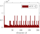
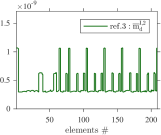
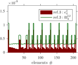
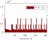
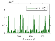
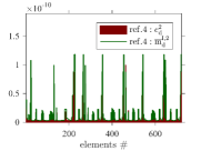
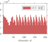
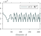
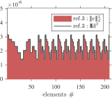
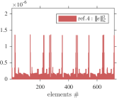
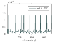
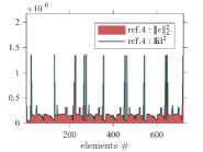
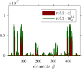
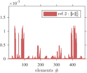
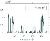
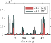
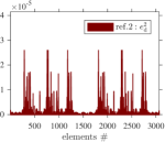
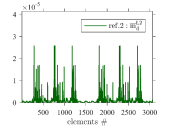
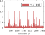
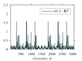
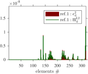
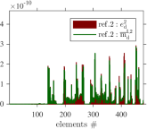
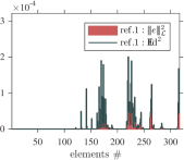
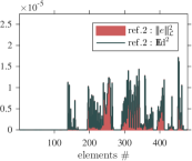
We also analyse the quantitative sharpness of the error indication provided by $\overline{\rm M}^{\rm I}$ and the local indicator generated by ${{\rm E\!\!\!Id}}$. This can be done by comparing local error contributions and local indicators w.r.t. numbered elements $K\in\mathcal{K}_{h}$ (see Figure 2 and 3). We can see that the local error contributions $e^{2}_{{\rm d},K}=\|\nabla_{x}e\|^{2}_{K}$ (red bars in the first column of Figure 2) are efficiently mimicked by the error indicators $\overline{\rm m}^{{\rm I},2}_{{\rm d},K}$ (green contour line in the second column). The resemblance of these distributions is even stronger emphasised in the third column of Figure 2, where plots from the first and the second columns overlap. The quantitative sharpness of the ${{\rm E\!\!\!Id}}$-distribution is analogously confirmed by Figure 3.

(a)

(b)

(c)

(d)

(e)

(f)

Figure 2: Example 1. Distribution of $e^{2}_{{\rm d},K}:=|\!|\nabla_{x}e|\!|^{2}_{K}$ and $\overline{\rm m}^{\rm I,2}_{{\rm d},K}:=\|\boldsymbol{y}_{h}-\nabla_{x}u_{h}\|^{2}_{K}$ w.r.t. refinements 2 and 3.

(a)

(b)

(c)

(d)

(e)

(f)

Figure 3: Example 1. Distribution of $|\!|\!|e|\!|\!|^{2}_{\mathcal{L},K}$ and ${\rm E\!\!\!Id}_{K}$ w.r.t. refinements 2 and 3.

6.2 Example 2

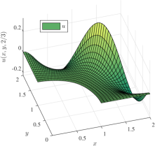
Next, we consider the example with the exact solution such that the change of the gradient depends on user-defined parameters. Let $Q=(0,1)^{2}$ be the unit square, and let the exact solution, the RHS, and the Dirichlet boundary conditions be chosen as follows:

$$u(x,t) =\sin(k_{1}\,\pi\,x)\,\sin(k_{2}\,\pi\,t)\quad (x,t) \in\overline{Q}=[0,1]^{2},$$

$$f(x,t) =\sin(k_{1}\,\pi\,x)\,(k_{2}\,\pi\,\cos(k_{2}\,\pi\,t)+k_{1}^{2}\,\pi^{2}\,\sin(k_{2}\,\pi\,t))\quad (x,t) \in{Q}=(0,1)^{2},$$

$$u_{0}(x,t) =0,\quad (x,t) \in{\overline{\Sigma}}_{0},$$

$$u_{D}(x,t) =0,\quad (x,t) \in\Sigma:=\partial\Omega\times(0,1).$$

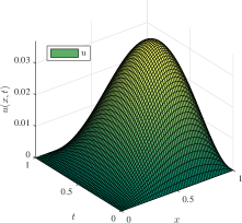
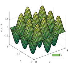
In the first part of the example (referred to Example 2-1), we chose the parameters as $k_{1}=k_{2}=1$. For such $k_{1}$ and $k_{2}$, the exact solution is illustrated in Figure 4a. The function $u_{h}$ is approximated by $S_{h}^{2}$, whereas $\boldsymbol{y}_{h}\in S_{7h}^{4}\oplus S_{7h}^{4}$ and $w_{h}\in S^{4}_{7h}$. We consider eight adaptive refinement steps ($N_{\rm ref}=8$) preceded by three global refinements ($N_{\rm ref,0}=3$) to generate the initial mesh. For the marking criterion, we use bulk marking with the parameter $\sigma=0.6$.

(a) $k_{1}=k_{2}=1$

(b) $k_{1}=6,k_{2}=3$

Figure 4: Example 2. Exact solution $u=\sin(k_{1}\,\pi\,x)\,\sin(k_{2}\,\pi\,t)$.

# ref.	$\|\nabla_{x}e\|_{Q}$	$I_{\rm eff}(\overline{\rm M}^{\rm I})$	$I_{\rm eff}(\overline{\rm M}^{\rm I\!I})$	$|\!|\!|e|\!|\!|_{s,h}$	$I_{\rm eff}(\overline{\rm M}^{\rm I}_{s,h})$	$|\!|\!|e|\!|\!|_{\mathcal{L}}$	$I_{\rm eff}({{\rm E\!\!\!Id}})$	e.o.c. ($|\!|\!|e|\!|\!|_{s,h}$)	e.o.c. ($|\!|\!|e|\!|\!|_{\mathcal{L}}$)
2	3.8987e-03	1.80	1.00	3.8988e-03	1.80	3.1934e-01	1.00	2.68	1.76
4	9.5149e-04	1.77	1.02	9.5149e-04	1.77	1.6041e-01	1.00	4.18	2.59
6	2.6155e-04	2.82	1.07	2.6170e-04	2.82	8.2550e-02	1.00	2.74	1.59
8	8.2844e-05	2.79	1.21	8.2854e-05	2.79	4.7088e-02	1.00	2.49	1.79

Table 6: Example 2-1. Efficiency of $\overline{\rm M}^{\rm I}$, $\overline{\rm M}^{\rm I\!I}$, $\overline{\rm M}^{\rm I}_{s,h}$, and ${{\rm E\!\!\!Id}}$ for $u_{h}\in S^{2}_{h}$, $\boldsymbol{y}_{h}\in S_{7h}^{4}\oplus S_{7h}^{4}$, and $w_{h}\in S^{4}_{7h}$, w.r.t. adaptive refinements (with the marking criterion ${\mathds{M}}_{\rm BULK}(0.6)$).

	d.o.f.			$t_{\rm as}$			$t_{\rm sol}$			$\tfrac{t_{\rm appr.}}{t_{\rm er.est.}}$
# ref.	$u_{h}$	$\boldsymbol{y}_{h}$	$w_{h}$	$u_{h}$	$\boldsymbol{y}_{h}$	$w_{h}$	$u_{h}$	$\boldsymbol{y}_{h}$	$w_{h}$
2	190	288	144	1.58e-01	6.92e-01	3.32e-01	1.51e-03	1.76e-03	3.94e-03	0.15
4	716	288	144	7.13e-01	7.20e-01	3.78e-01	2.24e-02	1.40e-03	2.34e-03	0. 65
6	2588	288	144	2.09e+00	7.06e-01	2.97e-01	1.73e-01	1.01e-03	2.20e-03	2.24
8	8303	288	144	8.27e+00	4.08e-01	3.08e-01	8.17e-01	8.65e-04	1.74e-03	5.92
				$t_{\rm as}(u_{h})$  :  $t_{\rm as}(\boldsymbol{y}_{h})$  :   $t_{\rm as}(w_{h})$			$t_{\rm sol}(u_{h})$   :  $t_{\rm sol}(\boldsymbol{y}_{h})$  :   $t_{\rm sol}(w_{h})$
				26.89	1.33	1.00	470.49	0.50	1.00

Table 7: Example 2-1. Assembling and solving time (in seconds) spent for the systems generating d.o.f. of $u_{h}\in S^{2}_{h}$, $\boldsymbol{y}_{h}\in S^{4}_{7h}\oplus S^{4}_{7h}$, and $w_{h}\in S^{4}_{7h}$ w.r.t. adaptive refinements (with the marking criterion ${\mathds{M}}_{\rm BULK}(0.6)$).

The resulting performance of the majorants and the error identity is presented in Table 6. It is again clear that $\overline{\rm M}^{\rm I\!I}$ is $1.8$–$2.8$ times sharper than $\overline{\rm M}^{\rm I}$. The performance of ${{\rm E\!\!\!Id}}$ remains sharp even though its values as well as the values of $|\!|\!|e|\!|\!|_{\mathcal{L}}$ decrease one order slower than $\overline{\rm M}^{\rm I}$ and $|\!|\!|e|\!|\!|$. At the same time, if we compare the effort spent on the reconstruction of $\boldsymbol{y}_{h}$ and $w_{h}$, we see from Table 7 that the approximation of $u_{h}$ takes longer. Total time expenses invested in $u_{h}$ are again compared to the costs of error-control in the last column of Table 7, where it is shown that ratios of such expenses reach $5.92$ on the last refinement step.

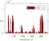
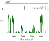
The comparison of the meshes in Figure 5 illustrates that the refinement based on $\|\nabla_{x}e\|_{Q}$ and the indicator $\overline{\rm m}^{\rm I}_{\rm d}$ (first and second columns) provide similar results. The same observation holds when we compare the meshes produced by refinement based on the distributions of $|\!|\!|e|\!|\!|_{\mathcal{L},K}$ and ${\rm E\!\!\!Id}_{K}$. The meshes, which we obtain using the majorant, mimic the topology of the meshes in the second column. The similarity of the meshes in the third and fourth columns provides clear evidence on the sharpness and the efficiency of ${\rm E\!\!\!Id}_{K}$, when the error indication is concerned. Moreover, the local error contribution $\|\nabla_{x}e\|_{K}$ and indicator $\overline{\rm m}^{\rm I}_{\rm d,K}$, as well as $|\!|\!|e|\!|\!|_{\mathcal{L},K}$ an ${\rm E\!\!\!Id}_{K}$, are compared in Figures 6 and 7, respectively. We illustrate the values of $\|\nabla_{x}e\|_{K}$ and $\overline{\rm m}^{\rm I}_{{\rm d},K}$ ($|\!|\!|e|\!|\!|_{\mathcal{L},K}$ and ${\rm E\!\!\!Id}_{K}$) on refinement step $2$.

(a) REF 5:
ref. based on $|\!|\!|e|\!|\!|_{h,s}$

(b) REF 5:
ref. based on $\overline{\rm m}^{\rm I}_{\rm d}$

(c) REF 5:
ref. based on $|\!|\!|e|\!|\!|_{\mathcal{L}}$

(d) REF 5:
ref. based on ${{\rm E\!\!\!Id}}$

(e) REF 7:
ref. based on $|\!|\!|e|\!|\!|_{h,s}$

(f) REF 7:
ref. based on $\overline{\rm m}^{\rm I}_{\rm d}$

(g) REF 7:
ref. based on $|\!|\!|e|\!|\!|_{\mathcal{L}}$

(h) REF 7:
ref. based on ${{\rm E\!\!\!Id}}$

Figure 5: Example 2-1. Comparison of meshes obtained by the refinement based on $|\!|\!|e|\!|\!|_{h,s}$, $\overline{\rm m}^{\rm I}_{\rm d}$, $|\!|\!|e|\!|\!|_{\mathcal{L}}$ and $|\!|\!|e|\!|\!|_{\mathcal{L}}$, where $\boldsymbol{y}_{h}\in S^{4}_{7h}\oplus S^{4}_{7h}$, and $w_{h}\in S^{4}_{7h}$, (with the marking criterion ${\mathds{M}}_{\rm BULK}(0.6)$).

(a)

(b)

(c)

Figure 6: Example 2-1. Local distribution of $e_{{\rm d},K}$ and $\overline{\rm m}_{{\rm d},K}$ on the refinement step $2$.

(a)

(b)

(c)

Figure 7: Example 2-1. Local distribution of $|\!|\!|e|\!|\!|_{\mathcal{L},K}$ and ${\rm E\!\!\!Id}_{K}$ on the refinement step $2$.

To conclude the evaluation of the error indication properties for this test-case, we compare the performance of the local error indicator generated by the majorant and local residual $\|\Delta_{x}u_{h}+f-\partial_{t}u_{h}\|^{2}_{K}$, $K\in\mathcal{K}_{h}$. Figure 8 demonstrates the similarity of the meshes obtained when the refinement is performed by local true error distribution (first column) and by the majorant error indicator (second column). At the same time, it emphasises that the refinement strategy provided by the local residual $\|\Delta_{x}u_{h}+f-\partial_{t}u_{h}\|^{2}_{K}$ is not as quantitatively exact. The corresponding meshes are illustrated in the third column of Figure 8 and differ from the meshes in the first column. Moreover, such an indicator has only heuristic nature and does not provide reliable error estimation.

(a) REF 5:
ref. based on $\|\nabla_{x}e\|^{2}_{K}$

(b) REF 5:
ref. based on $\overline{\rm m}^{\rm I}_{{\rm d},K}$

(c) REF 5:
ref. based on $\|\Delta_{x}u_{h}+f-\partial_{t}u_{h}\|^{2}_{K}$

(d) REF 6:
ref. based on $\|\nabla_{x}e\|^{2}_{K}$

(e) REF 6:
ref. based on $\overline{\rm m}^{\rm I}_{{\rm d},K}$

(f) REF 6:
ref. based on $\|\Delta_{x}u_{h}+f-\partial_{t}u_{h}\|^{2}_{K}$

(g) REF 7:
ref. based on $\|\nabla_{x}e\|^{2}_{K}$

(h) REF 7:
ref. based on $\overline{\rm m}^{\rm I}_{{\rm d},K}$

(i) REF 7:
ref. based on $\|\Delta_{x}u_{h}+f-\partial_{t}u_{h}\|^{2}_{K}$

Figure 8: Example 2-1. Comparison of meshes obtained by the refinement based on local contributions $\|\nabla_{x}e\|^{2}_{K}$, $\overline{\rm m}^{\rm I}_{\rm d,K}$, and residual $\|\Delta u_{h}+f-\partial_{t}u_{h}\|^{2}_{K}$, $K\in\mathcal{K}_{h}$, where $\boldsymbol{y}_{h}\in S^{4}_{7h}\oplus S^{4}_{7h}$, and $w_{h}\in S^{4}_{7h}$, (with the marking criterion ${\mathds{M}}_{\rm BULK}(0.6)$).

Next, let us consider a more complicated case with $k_{1}=6$ and $k_{2}=3$ (see Figure 4b). We start with a configuration, where the initial mesh is obtained by four global refinements ($N^{0}_{\rm ref}=4$), and we proceed with six adaptive steps ($N_{\rm ref}=6$) using the $\mathds{M}_{\rm BULK}(\sigma)$ marking criterion with $\sigma=0.6$. The obtained efficiency indices characterising all majorants and error identity are presented in Table 8. Here, the auxiliary functions $\boldsymbol{y}_{h}$ and $w_{h}$ are taken from the approximation spaces $S^{7}_{7h}\oplus S^{7}_{7h}$ and $S^{7}_{7h}$, respectively. We see that the performance of $\overline{\rm M}^{\rm I}_{s,h}$ is identical to that of the majorant $\overline{\rm M}^{\rm I}$, since $\theta$ from the space-time IgA scheme is set to zero in this example. The numerical performance of the majorant corresponding to the advanced discretisation scheme with parameter $\delta_{h}$ scaled proportionally to the local size of the element $h_{K}$ will be discussed in the follow-up report.

# ref.	$\|\nabla_{x}e\|_{Q}$	$I_{\rm eff}(\overline{\rm M}^{\rm I})$	$I_{\rm eff}(\overline{\rm M}^{\rm I\!I})$	$|\!|\!|e|\!|\!|_{s,h}$	$I_{\rm eff}(\overline{\rm M}^{\rm I}_{s,h})$	$|\!|\!|e|\!|\!|_{\mathcal{L}}$	$I_{\rm eff}({{\rm E\!\!\!Id}})$	e.o.c. ($|\!|\!|e|\!|\!|_{s,h}$)	e.o.c. ($|\!|\!|e|\!|\!|_{\mathcal{L}}$)
2	1.7936e-01	1.15	1.01	1.7936e-01	1.15	3.2970e+01	1.00	2.18	1.20
4	2.8466e-02	1.15	1.03	2.8466e-02	1.15	1.3901e+01	1.00	2.41	0.83
6	7.3156e-03	1.29	1.11	7.3156e-03	1.29	7.2587e+00	1.00	1.61	0.52
8	1.9064e-03	2.02	1.32	1.9064e-03	2.02	3.6573e+00	1.00	2.21	0.82

Table 8: Example 2-2. Efficiency of $\overline{\rm M}^{\rm I}$, $\overline{\rm M}^{\rm I\!I}$, $\overline{\rm M}^{\rm I}_{s,h}$, and ${{\rm E\!\!\!Id}}$ for $u_{h}\in S^{2}_{h}$, $\boldsymbol{y}_{h}\in S^{7}_{7h}\oplus S^{7}_{7h}$ and $w_{h}\in S^{7}_{7h}$, w.r.t. adaptive refinement steps (with the marking criterion ${\mathds{M}}_{\rm BULK}(0.6)$).

	d.o.f.			$t_{\rm as}$			$t_{\rm sol}$			$\tfrac{t_{\rm appr.}}{t_{\rm er.est.}}$
# ref.	$u_{h}$	$\boldsymbol{y}_{h}$	$w_{h}$	$u_{h}$	$\boldsymbol{y}_{h}$	$w_{h}$	$u_{h}$	$\boldsymbol{y}_{h}$	$w_{h}$
2	940	1058	529	7.96e-01	2.03e+01	1.02e+01	2.41e-02	5.16e-02	5.92e-02	0.03
4	5590	1058	529	5.64e+00	1.80e+01	1.01e+01	4.56e-01	4.63e-02	5.65e-02	0.22
6	21089	1058	529	3.14e+01	1.81e+01	1.01e+01	3.70e+00	3.12e-02	5.51e-02	1.24
8	67043	1058	529	2.06e+02	1.82e+01	1.23e+01	1.64e+01	4.59e-02	7.40e-02	7.26
				$t_{\rm as}(u_{h})$  :  $t_{\rm as}(\boldsymbol{y}_{h})$  :   $t_{\rm as}(w_{h})$			$t_{\rm sol}(u_{h})$   :  $t_{\rm sol}(\boldsymbol{y}_{h})$  :   $t_{\rm sol}(w_{h})$
				16.76	1.48	1.00	221.53	0.62	1.00

Table 9: Example 2-2. Assembling and solving time (in seconds) spent for the systems generating d.o.f. of $u_{h}\in S^{2}_{h}$, $\boldsymbol{y}_{h}\in S^{7}_{7h}\oplus S^{7}_{7h}$, and $w_{h}\in S^{7}_{7h}$ w.r.t. adaptive refinement steps (with the marking criterion ${\mathds{M}}_{\rm BULK}(0.6)$).

A comparison of the meshes corresponding to different refinement criteria is presented in Figure 9. The first two columns contain the meshes produced by the refinement based on ${\rm e}_{\rm d}$ and $\overline{\rm m}^{\rm I}_{\rm d}$, whereas the third and fourth columns correspond to the adaptive meshes obtained on the steps 3 and 4 using local distributions of $|\!|\!|e|\!|\!|_{\mathcal{L},K}$ and ${{\rm E\!\!\!Id}}_{K}$ for the refinement criterion. It is clear from the plots that the meshes related to ${{\rm E\!\!\!Id}}$-based refinement are denser than the meshes in the second column. Nevertheless, the error identity suggests similar areas of the mesh refinement. Therefore, it can be used as effectively as $\overline{\rm m}^{\rm I}_{\rm d}$ for mesh-adaptation. Moreover, Figure 10 confirms that $\overline{\rm m}^{\rm I}_{{\rm d},K}$ and ${{\rm E\!\!\!Id}}_{K}$ are quantitatively sharp when it comes to estimating ${\rm e}_{{\rm d},K}$ and $|\!|\!|e|\!|\!|_{\mathcal{L},K}$, respectively.

(a) REF 3:
ref. based on ${\rm e}_{\rm d}$

(b) REF 3:
ref. based on $\overline{\rm m}^{\rm I}_{\rm d}$

(c) REF 3:
ref. based on $|\!|\!|e|\!|\!|_{\mathcal{L}}$

(d) REF 3:
ref. based on ${{\rm E\!\!\!Id}}$

(e) REF 4:
ref. based on ${\rm e}_{\rm d}$

(f) REF 4:
ref. based on $\overline{\rm m}^{\rm I}_{\rm d}$

(g) REF 4:
ref. based on $|\!|\!|e|\!|\!|_{\mathcal{L}}$

(h) REF 4:
ref. based on ${{\rm E\!\!\!Id}}$

Figure 9: Example 2-2. Comparison of the meshes obtained by refinement based on ${\rm e}_{\rm d}$, $\overline{\rm m}^{\rm I}_{\rm d}$, $|\!|\!|e|\!|\!|_{\mathcal{L}}$, and ${{\rm E\!\!\!Id}}$ for $u_{h}\in S^{2}_{h}$, $\boldsymbol{y}_{h}\in S^{7}_{7h}\oplus S^{7}_{7h}$, and $w_{h}\in S^{7}_{7h}$, (with the marking criterion ${\mathds{M}}_{\rm BULK}(0.6)$).

(a)

(b)

(c)

(d)

Figure 10: Example 2-2. Distribution of $e_{{\rm d},K}$ and $\overline{\rm m}_{{\rm d},K}$ as well as $|\!|\!|e|\!|\!|_{\mathcal{L},K}$ and ${\rm E\!\!\!Id}_{K}$ on the refinement step $2$.

6.3 Example 3

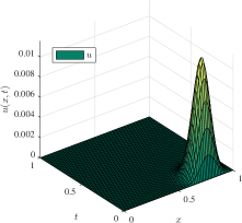
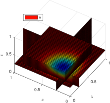
As another standard test case, we consider an example with a sharp local Gaussian peak in the exact solution. Let $Q:=(0,1)^{2}$, and the solution to be defined by

$$u(x,t) =(x^{2}-x)\,(t^{2}-t)\,e^{-100\,|(x,t)-(0.8,0.05)|}, \quad(x,t)\in\overline{Q},$$

where the peak is located in the point $(x,t)=(0.8,0.05)$, see Figure 11a. Then $f$ is computed by substituting $u$ into (1). The Dirichlet boundary conditions are obviously homogeneous.

(a)

(b)

Figure 11: Example 3. (a) Exact solution $u=x\,(x-1)\,t\,(t-1)\,e^{-100\,|(x,t)-(0.8,0.05)|}$. (b) Exact solution
$u=x\,(x-1)\,y\,(y-1)\,t\,(t-1)\,e^{-100\,|(x,y,t)-(0.25,0.25,0.25)|}$.

For this example, we consider only an adaptive refinement procedure. For the discretisation spaces, we use our standard setting, i.e., $u_{h}\in S^{2}_{h}$ for the primal variable, as well as $\boldsymbol{y}_{h}\in S^{3}_{h}\oplus S^{3}_{h}$ and $w_{h}\in S^{3}_{h}$ for the auxiliary functions. We start with four initial global refinements ($N^{0}_{\rm ref}=4$), and continue with seven adaptive steps ($N_{\rm ref}=7$). As marking criteria, we choose $\mathds{M}_{\rm BULK}(\sigma)$ with bulk parameter $\sigma=0.6$.

The analysis of the quantitative efficiency of the majorants and the error identity in terms of error estimation is provided in Table 10, which confirms that $\overline{\rm M}^{\rm I\!I}$ is twice as sharp as that of $\overline{\rm M}^{\rm I}$, and the error identity sharply predicts the exact error $|\!|\!|e|\!|\!|_{\mathcal{L}}$. When it comes to the time efficiency summarised in Table 11, we see that the assembling of matrices for the $\boldsymbol{y}_{h}$ and $w_{h}$ is 3 - 4 times more time-consuming. However, the solution of the corresponding systems is 1.4 - 3 times faster.

# ref.	$\|\nabla_{x}e\|_{Q}$	$I_{\rm eff}(\overline{\rm M}^{\rm I})$	$I_{\rm eff}(\overline{\rm M}^{\rm I\!I})$	$|\!|\!|e|\!|\!|_{s,h}$	$I_{\rm eff}(\overline{\rm M}^{\rm I}_{s,h})$	$|\!|\!|e|\!|\!|_{\mathcal{L}}$	$I_{\rm eff}({{\rm E\!\!\!Id}})$	e.o.c. ($|\!|\!|e|\!|\!|_{s,h}$)	e.o.c. ($|\!|\!|e|\!|\!|_{\mathcal{L}}$)
3	6.1181e-02	1.58	1.24	6.1181e-02	1.58	1.8482e+01	1.00	2.00	1.07
5	1.4192e-02	1.32	1.12	1.4192e-02	1.32	9.0808e+00	1.00	2.77	1.75
7	4.1402e-03	1.27	1.07	4.1402e-03	1.27	4.8937e+00	1.00	2.46	1.71

Table 10: Example 3. Efficiency of $\overline{\rm M}^{\rm I}$, $\overline{\rm M}^{\rm I\!I}$, $\overline{\rm M}^{\rm I}_{s,h}$, and ${{\rm E\!\!\!Id}}$ for $u_{h}\in S^{2}_{h}$, $\boldsymbol{y}_{h}\in S_{h}^{3}\oplus S_{h}^{3}$, and $w_{h}\in S^{3}_{h}$, w.r.t. adaptive refinements (with the marking criterion ${\mathds{M}}_{\rm BULK}(0.6)$).

	d.o.f.			$t_{\rm as}$			$t_{\rm sol}$			$\tfrac{t_{\rm appr.}}{t_{\rm er.est.}}$
# ref.	$u_{h}$	$\boldsymbol{y}_{h}$	$w_{h}$	$u_{h}$	$\boldsymbol{y}_{h}$	$w_{h}$	$u_{h}$	$\boldsymbol{y}_{h}$	$w_{h}$
1	324	722	361	1.90e-01	1.01e+00	6.23e-01	3.43e-03	2.54e-03	1.03e-02	0.12
3	543	1142	571	4.31e-01	2.95e+00	1.61e+00	1.33e-02	1.65e-02	4.06e-02	0.10
5	1167	2342	1171	9.20e-01	7.79e+00	3.90e+00	5.62e-02	8.07e-02	1.71e-01	0.08
7	4006	7742	3871	5.43e+00	3.01e+01	1.83e+01	7.43e-01	5.12e-01	1.42e+00	0.12
				$t_{\rm as}(u_{h})$  :  $t_{\rm as}(\boldsymbol{y}_{h})$  :   $t_{\rm as}(w_{h})$			$t_{\rm sol}(u_{h})$   :  $t_{\rm sol}(\boldsymbol{y}_{h})$  :   $t_{\rm sol}(w_{h})$
				0.30	1.65	1.00	0.52	0.36	1.00	0.12

Table 11: Example 3. Assembling and solving time (in seconds) spent for the systems generating d.o.f. of $u_{h}\in S^{2}_{h}$, $\boldsymbol{y}_{h}\in S^{3}_{h}\oplus S^{3}_{h}$, and $w_{h}\in S^{3}_{h}$ w.r.t. adaptive refinements (with the marking criterion ${\mathds{M}}_{\rm BULK}(0.6)$).

Coming back to the error indication properties of the majorant and the error identity, we analyse the meshes presented in Figure 12. The first two columns compare the meshes produced by the refinement based on ${\rm e}_{\rm d}$ and $\overline{\rm m}^{\rm I}_{\rm d}$. The third and the fourth columns illustrate practically matching meshes produced by values of $|\!|\!|e|\!|\!|_{\mathcal{L}}$ and ${{\rm E\!\!\!Id}}$. This test demonstrates that both $\overline{\rm m}^{\rm I}_{{\rm d}}$ and ${{\rm E\!\!\!Id}}$ can be used for error indication and efficient mesh refinement algorithm. In particular, the error identity is suited for the cases when we can not afford any time overhead for error analysis.

(a) REF 4:
ref. based on ${\rm e}_{\rm d}$

(b) REF 4:
ref. based on $\overline{\rm m}^{\rm I}_{\rm d}$

(c) REF 4:
ref. based on $|\!|\!|e|\!|\!|_{\mathcal{L}}$

(d) REF 4:
ref. based on ${{\rm E\!\!\!Id}}$

(e) REF 5:
ref. based on ${\rm e}_{\rm d}$

(f) REF 5:
ref. based on $\overline{\rm m}^{\rm I}_{\rm d}$

(g) REF 5:
ref. based on $|\!|\!|e|\!|\!|_{\mathcal{L}}$

(h) REF 5:
ref. based on ${{\rm E\!\!\!Id}}$

Figure 12: Example 3. Comparison of the meshes obtained by refinement based on ${\rm e}_{\rm d}$, $\overline{\rm m}^{\rm I}_{\rm d}$, $|\!|\!|e|\!|\!|_{\mathcal{L}}$, and ${{\rm E\!\!\!Id}}$ for $u_{h}\in S^{2}_{h}$, $\boldsymbol{y}_{h}\in S_{h}^{3}\oplus S_{h}^{3}$, and $w_{h}\in S_{h}^{3}$, w.r.t. refinement steps 4 and 5.

(a)

(b)

(c)

(d)

Figure 13: Example 3. Distribution of ${\rm e}_{{\rm d},K}$, $\overline{\rm m}^{\rm I}_{{\rm d},K}$, as well as $|\!|\!|e|\!|\!|_{\mathcal{L},K}$, and ${\rm E\!\!\!Id}_{K}$ on the refinement step 1 and 2.

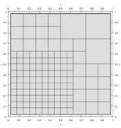
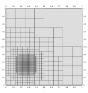
To emphasise on the advantages of the space-time approach, we consider an analogous example for $d=2$, i.e., $Q:=(0,1)^{3}$, such that the solution is defined by

$$u(x,y,t) =(x^{2}-x)\,(y^{2}-y)\,(t^{2}-t)\,e^{-100\,|(x,y,t)-(0.25,0.25,0.25)|}, \quad(x,y,t)\in\overline{Q}.$$

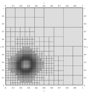
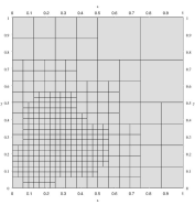
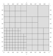
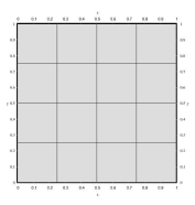
Here, the Gaussian peak is located in the point $(x,y,t)=(0.250.25,0.25)$. Analogously, $f$ is computed by substituting $u$ into (1), as well as the Dirichlet boundary conditions remains homogeneous. Figure 14 illustrates $2$-dimensional meshes obtained by slicing $3$-dimensional meshes (in space and time) along the time variable. Figures demonstrate the advantage of the adaptive space-time approach over the time-stepping methods, which always have to consider refining or coarsening on subsequent time step. It is also worth emphasising on the universality of the applied functional error estimates w.r.t. to any discretisation. To our knowledge, it is the only approach, which allows fully unstructured discretisation in space and time for evolutionary equations. Application of functional error estimates to FEM and their corresponding numerical properties are studied in [18].

(a) $t=0$

(b) $t=0.125$

(c) $t=0.25$

(d) $t=0.5$

(e) $t=0.75$

(f) $t=1.0$

Figure 14: Example 3. Meshes obtained by the space-time refinement based on $\overline{\rm m}^{\rm I}_{\rm d}$ for $u_{h}\in S^{2}_{h}$, $\boldsymbol{y}_{h}\in S_{h}^{3}\oplus S_{h}^{3}$, and $w_{h}\in S_{h}^{3}$, w.r.t. $t=\big{\{}0,0.125,0.25,0.5,0.75,1.0\big{\}}$.

6.4 Example 4

Finally, in the last example, we test functional error estimates on the three-dimensional space-time cylinder $Q=\Omega_{\,\leavevmode\hbox to6.09pt{\vbox to6.09pt{\pgfpicture\makeatletter\hbox{\hskip 0.2pt\lower-0.2pt\hbox to0.0pt{\pgfsys@beginscope\pgfsys@invoke{ }\definecolor{pgfstrokecolor}{rgb}{0,0,0}\pgfsys@color@rgb@stroke{0}{0}{0}\pgfsys@invoke{ }\pgfsys@color@rgb@fill{0}{0}{0}\pgfsys@invoke{ }\pgfsys@setlinewidth{0.4pt}\pgfsys@invoke{ }\nullfont\hbox to0.0pt{\pgfsys@beginscope\pgfsys@invoke{ }{{}}{}{{}}{} {}{}{{{}{}{}{}}}{} {} {}{} {}{}{{{}{}{}{}}}{} {} {}{} {}{}\pgfsys@moveto{2.84544pt}{0.0pt}\pgfsys@lineto{5.69089pt}{0.0pt}\pgfsys@curveto{5.69089pt}{3.14304pt}{3.14304pt}{5.69089pt}{0.0pt}{5.69089pt}\pgfsys@lineto{0.0pt}{2.84544pt}\pgfsys@curveto{1.5715pt}{2.84544pt}{2.84544pt}{1.5715pt}{2.84544pt}{0.0pt}\pgfsys@closepath\pgfsys@stroke\pgfsys@invoke{ } \pgfsys@invoke{\lxSVG@closescope }\pgfsys@endscope{}{}{}\hss}\pgfsys@discardpath\pgfsys@invoke{\lxSVG@closescope }\pgfsys@endscope\hss}}\lxSVG@closescope\endpgfpicture}}}\times(0,T)$, where $\Omega_{\leavevmode\hbox to6.09pt{\vbox to6.09pt{\pgfpicture\makeatletter\hbox{\hskip 0.2pt\lower-0.2pt\hbox to0.0pt{\pgfsys@beginscope\pgfsys@invoke{ }\definecolor{pgfstrokecolor}{rgb}{0,0,0}\pgfsys@color@rgb@stroke{0}{0}{0}\pgfsys@invoke{ }\pgfsys@color@rgb@fill{0}{0}{0}\pgfsys@invoke{ }\pgfsys@setlinewidth{0.4pt}\pgfsys@invoke{ }\nullfont\hbox to0.0pt{\pgfsys@beginscope\pgfsys@invoke{ }{{}}{}{{}}{} {}{}{{{}{}{}{}}}{} {} {}{} {}{}{{{}{}{}{}}}{} {} {}{} {}{}\pgfsys@moveto{2.84544pt}{0.0pt}\pgfsys@lineto{5.69089pt}{0.0pt}\pgfsys@curveto{5.69089pt}{3.14304pt}{3.14304pt}{5.69089pt}{0.0pt}{5.69089pt}\pgfsys@lineto{0.0pt}{2.84544pt}\pgfsys@curveto{1.5715pt}{2.84544pt}{2.84544pt}{1.5715pt}{2.84544pt}{0.0pt}\pgfsys@closepath\pgfsys@stroke\pgfsys@invoke{ } \pgfsys@invoke{\lxSVG@closescope }\pgfsys@endscope{}{}{}\hss}\pgfsys@discardpath\pgfsys@invoke{\lxSVG@closescope }\pgfsys@endscope\hss}}\lxSVG@closescope\endpgfpicture}}}$ is of a quarter-annulus shape, and the final time of the time interval is $1$. The exact solution is defined by

$$u(x,y,t) =(1-x)\,x^{2}\,(1-y)\,y^{2}\,(1-t)\,t^{2}, \quad(x,y,t) \in\overline{Q}:=\overline{\Omega}_{\leavevmode\hbox to6.09pt{\vbox to6.09pt{\pgfpicture\makeatletter\hbox{\hskip 0.2pt\lower-0.2pt\hbox to0.0pt{\pgfsys@beginscope\pgfsys@invoke{ }\definecolor{pgfstrokecolor}{rgb}{0,0,0}\pgfsys@color@rgb@stroke{0}{0}{0}\pgfsys@invoke{ }\pgfsys@color@rgb@fill{0}{0}{0}\pgfsys@invoke{ }\pgfsys@setlinewidth{0.4pt}\pgfsys@invoke{ }\nullfont\hbox to0.0pt{\pgfsys@beginscope\pgfsys@invoke{ }{{}}{}{{}}{} {}{}{{{}{}{}{}}}{} {} {}{} {}{}{{{}{}{}{}}}{} {} {}{} {}{}\pgfsys@moveto{2.84544pt}{0.0pt}\pgfsys@lineto{5.69089pt}{0.0pt}\pgfsys@curveto{5.69089pt}{3.14304pt}{3.14304pt}{5.69089pt}{0.0pt}{5.69089pt}\pgfsys@lineto{0.0pt}{2.84544pt}\pgfsys@curveto{1.5715pt}{2.84544pt}{2.84544pt}{1.5715pt}{2.84544pt}{0.0pt}\pgfsys@closepath\pgfsys@stroke\pgfsys@invoke{ } \pgfsys@invoke{\lxSVG@closescope }\pgfsys@endscope{}{}{}\hss}\pgfsys@discardpath\pgfsys@invoke{\lxSVG@closescope }\pgfsys@endscope\hss}}\lxSVG@closescope\endpgfpicture}}}\times[0,1],$$

see Figure 15. The RHS $f(x,y,t)$, $(x,y,t)\in Q:={\Omega}_{\leavevmode\hbox to6.09pt{\vbox to6.09pt{\pgfpicture\makeatletter\hbox{\hskip 0.2pt\lower-0.2pt\hbox to0.0pt{\pgfsys@beginscope\pgfsys@invoke{ }\definecolor{pgfstrokecolor}{rgb}{0,0,0}\pgfsys@color@rgb@stroke{0}{0}{0}\pgfsys@invoke{ }\pgfsys@color@rgb@fill{0}{0}{0}\pgfsys@invoke{ }\pgfsys@setlinewidth{0.4pt}\pgfsys@invoke{ }\nullfont\hbox to0.0pt{\pgfsys@beginscope\pgfsys@invoke{ }{{}}{}{{}}{} {}{}{{{}{}{}{}}}{} {} {}{} {}{}{{{}{}{}{}}}{} {} {}{} {}{}\pgfsys@moveto{2.84544pt}{0.0pt}\pgfsys@lineto{5.69089pt}{0.0pt}\pgfsys@curveto{5.69089pt}{3.14304pt}{3.14304pt}{5.69089pt}{0.0pt}{5.69089pt}\pgfsys@lineto{0.0pt}{2.84544pt}\pgfsys@curveto{1.5715pt}{2.84544pt}{2.84544pt}{1.5715pt}{2.84544pt}{0.0pt}\pgfsys@closepath\pgfsys@stroke\pgfsys@invoke{ } \pgfsys@invoke{\lxSVG@closescope }\pgfsys@endscope{}{}{}\hss}\pgfsys@discardpath\pgfsys@invoke{\lxSVG@closescope }\pgfsys@endscope\hss}}\lxSVG@closescope\endpgfpicture}}}\times(0,1)$, is computed based on the substitution of $u$ into the equation (1) and the Dirichlet boundary conditions are defined as $u_{D}=u$ on $\Sigma$.

(a)

(b)

Figure 15: Example 4. (a) Exact solution $u=(1-x)\,x^{2}\,(1-y)\,y^{2}\,(1-t)\,t^{2}$. (b) $u$ at the time moment $t=\tfrac{2}{3}$.

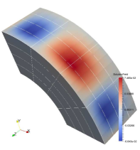
The initial mesh for the test is generated by one uniform refinement $N^{0}_{\rm ref}=1$. We start the analysis from Table 12, where the performance of the studied error estimates is illustrated for both uniform and adaptive refinement strategies. It is easy to see that all majorants have adequate performance, taking into account that the auxiliary functions $\boldsymbol{y}_{h}\in\oplus^{3}S_{3h}^{3}$ and $w_{h}\in S^{3}_{3h}$ are from spline spaces of just one order higher than the spline space for $u_{h}$. Such choice of the spaces is beneficial when the time expenditure on error estimation is concerned. Table 13 confirms that assembling and solving of the systems reconstructing d.o.f. of $u_{h}$ requires more time than assembling and solving routines for the systems generating $\boldsymbol{y}_{h}$ and $w_{h}$.

# ref.	$\|\nabla_{x}e\|_{Q}$	$I_{\rm eff}(\overline{\rm M}^{\rm I})$	$I_{\rm eff}(\overline{\rm M}^{\rm I\!I})$	$|\!|\!|e|\!|\!|_{s,h}$	$I_{\rm eff}(\overline{\rm M}^{\rm I}_{s,h})$	$|\!|\!|e|\!|\!|_{\mathcal{L}}$	$I_{\rm eff}({{\rm E\!\!\!Id}})$	e.o.c. ($|\!|\!|e|\!|\!|_{s,h}$)	e.o.c. ($|\!|\!|e|\!|\!|_{\mathcal{L}}$)
uniform refinement
3	9.6674e-03	6.17	5.37	9.6675e-03	6.18	1.9361e-01	1.00	3.30	1.46
4	2.1555e-03	6.89	5.04	2.1555e-03	6.90	9.0086e-02	1.00	2.55	1.30
5	5.2154e-04	3.35	2.67	5.2154e-04	3.39	4.4046e-02	1.00	2.23	1.13
6	1.2926e-04	2.04	1.67	1.2926e-04	2.15	2.1892e-02	1.00	2.10	1.05
adaptive refinement using bulk marking criterion $\sigma=0.4$
3	9.6919e-03	6.16	5.36	9.6919e-03	6.16	1.9385e-01	1.00	3.56	1.57
4	2.4997e-03	5.98	4.38	2.4997e-03	5.98	9.4309e-02	1.00	3.25	1.73
5	9.4272e-04	2.28	1.78	9.4272e-04	2.28	5.4120e-02	1.00	1.79	1.02
6	2.5862e-04	1.52	1.29	2.5862e-04	1.52	3.0451e-02	1.00	2.88	1.28

Table 12: Example 4. Efficiency of $\overline{\rm M}^{\rm I}$, $\overline{\rm M}^{\rm I\!I}$, $\overline{\rm M}^{\rm I}_{s,h}$, and ${{\rm E\!\!\!Id}}$ for $u_{h}\in S^{2}_{h}$, $\boldsymbol{y}_{h}\in\oplus^{3}S_{2h}^{3}$, and $w_{h}\in S^{3}_{2h}$, w.r.t. uniform refinement and adaptive refinement steps.

	d.o.f.			$t_{\rm as}$			$t_{\rm sol}$			$\tfrac{t_{\rm appr.}}{t_{\rm er.est.}}$
# ref.	$u_{h}$	$\boldsymbol{y}_{h}$	$w_{h}$	$u_{h}$	$\boldsymbol{y}_{h}$	$w_{h}$	$u_{h}$	$\boldsymbol{y}_{h}$	$w_{h}$
uniform refinement
2	216	375	125	5.68e-02	9.14e-02	4.70e-02	1.12e-03	9.10e-03	2.15e-04	0.39
3	1000	375	125	3.87e-01	9.34e-02	4.51e-02	4.14e-02	1.40e-02	2.39e-04	2.81
4	5832	1029	343	2.97e+00	6.94e-01	2.62e-01	3.49e+00	1.79e-01	3.62e-03	5.67
5	39304	3993	1331	2.36e+01	5.74e+00	1.96e+00	1.09e+02	3.77e+00	1.67e-01	11.40
6	287496	20577	6859	1.80e+02	2.91e+01	9.53e+00	1.12e+04	5.17e+01	6.76e+00	117.73
				$t_{\rm as}(u_{h})$  :  $t_{\rm as}(\boldsymbol{y}_{h})$  :   $t_{\rm as}(w_{h})$			$t_{\rm sol}(u_{h})$   :  $t_{\rm sol}(\boldsymbol{y}_{h})$  :   $t_{\rm sol}(w_{h})$
				18.93	3.06	1.00	1664.71	7.64	1.00
adaptive refinement using bulk marking criterion $\sigma=0.4$ ($N_{\rm ref,0}$ = 1)
2	216	375	125	5.55e-01	5.01e-01	4.15e-01	8.41e-04	1.08e-02	3.65e-04	0.60
3	894	375	125	5.48e+00	5.79e-01	3.99e-01	2.28e-02	7.36e-03	2.38e-04	5.58
4	3127	1029	343	4.60e+01	5.15e+00	3.19e+00	5.16e-01	1.75e-01	2.68e-03	5.46
5	15990	3993	1331	2.25e+02	3.92e+01	2.29e+01	1.96e+01	3.41e+00	1.02e-01	3.72
6	61390	20577	6859	1.22e+03	2.33e+02	1.83e+02	3.85e+02	5.86e+01	6.63e+00	3.32
				$t_{\rm as}(u_{h})$  :  $t_{\rm as}(\boldsymbol{y}_{h})$  :   $t_{\rm as}(w_{h})$			$t_{\rm sol}(u_{h})$   :  $t_{\rm sol}(\boldsymbol{y}_{h})$  :   $t_{\rm sol}(w_{h})$
				6.63	1.27	1.00	58.07	8.84	1.00

Table 13: Example 4. Assembling and solving time (in seconds) spent for the systems generating d.o.f. of $u_{h}\in S^{3}_{3h}$ $\boldsymbol{y}_{h}\in\oplus^{3}S^{3}_{3h}$, and $w_{h}\in S^{3}_{3h}$ w.r.t (a) uniform refinements and (b) adaptive refinements (using bulk marking criterion with $\sigma=0.4$).

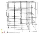
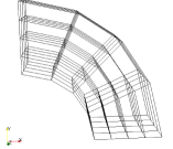
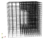
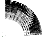
All the numerical results presented below are obtained for the bulk marking criterion with the parameter $\sigma=0.4$. Figure 16 presents an evolution of the adaptive meshes discretising the parametric space-time cylinder $\hat{Q}$ (left column) and the corresponding meshes discretising $Q$ (right column). From the graphics presented, we can see that the refinement is localised in the area close to the lateral surface of the quarter-annulus with the radius two. This can be explained by fast changes in the solution appearing close to this ‘outer’ surface, see $u$ at the time $t=\tfrac{2}{3}$ in Figure 15b.

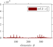
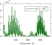
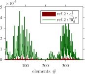
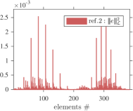
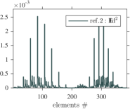
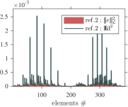
Finally, we provide a quantitative comparison of the local distributions ${\rm e}_{{\rm d},K}$ and $\overline{\rm m}^{\rm I}_{{\rm d},K}$ as well as $|\!|\!|e|\!|\!|_{\mathcal{L},K}$ and ${\rm E\!\!\!Id}_{K}$ in Figure 17. The first two columns of these graphics expose the quantities individually, and the last column contains plots with overlapped distributions of the error and the error indicator. In Figure 17, we see that $\overline{\rm m}^{\rm I}_{{\rm d},K}$ overestimates ${\rm e}_{{\rm d},K}$, whereas the local indication of ${\rm E\!\!\!Id}_{K}$ is sharper w.r.t the element-wise contributions $|\!|\!|e|\!|\!|_{\mathcal{L},K}$.

(a) ref. # 1:  $\hat{\Omega}$ and $\hat{\mathcal{K}}_{h}$

(b) ref. # 1:  ${\Omega}$ and ${\mathcal{K}}_{h}$

(c) ref. # 3:  $\hat{\Omega}$ and $\hat{\mathcal{K}}_{h}$

(d) ref. # 3:  ${\Omega}$ and ${\mathcal{K}}_{h}$

Figure 16: Example 4. Comparison of meshes on the physical and parametric domains w.r.t. adaptive refinement steps, criterion ${\mathds{M}}_{{\rm\bf BULK}}(0.6)$.

(a)

(b)

(c)

(d)

(e)

(f)

Figure 17: Example 4. Distribution of ${\rm e}_{{\rm d},K}$, $\overline{\rm m}^{\rm I}_{{\rm d},K}$ (first row) as well as $|\!|\!|e|\!|\!|_{\mathcal{L},K}$ and ${\rm E\!\!\!Id}_{K}$ (second row) on the refinement step 2.

6.5 Example 5 (solution with singularity w.r.t. $x$-coordinates)

(a) $u(x,y,1)$

(b) $\mathcal{K}_{h}$ defined on $\Omega$

Figure 18: Ex. 6.5. (a) Exact solution $u=r^{1/3}\,\sin\theta\,\phi(1)$. (b) Initial geometry with Greville’s points with double control points at the corners and a corresponding mesh generated with $C^{1}$-continuous geometrical mapping.

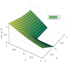
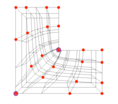
In order to show how error estimates handle solutions with singularities, we consider a classical benchmark example on a two-dimensional L-shaped domain extended linearly in time to a cylinder $Q=\Omega\times(0,T)$, where $\Omega:=\big{(}(-1,1)\times(-1,1)\big{)}\backslash\big{(}[0,1)\times[0,1)\big{)}$ and $T=2$. The Dirichlet BCs are defined on $\Sigma$ by the Dirichlet data $u_{D}=r^{1/3}\,\sin(\theta)$, where

$$r={r(x,y)=}(x^{2}+y^{2})\quad\mbox{and}\quad\theta={\theta(x,y)=}\begin{cases}\tfrac{1}{3}\,(2\,{\rm atan2}(y,x)-\pi)\;\;\mbox{for}\;\;y>0,\\[-1.0pt] \tfrac{1}{3}\,(2\,{\rm atan2}(y,x)+3\,\pi)\;\;\mbox{for}\;\;y\leq 0.\end{cases}$$

The corresponding exact solution

$$u(x,y,t)=r(x,y)^{1/3}\,\sin(\theta(x,y))\,\phi(t),\quad\mbox{where}\quad\phi(t)=t^{2}+t+1,\quad(x,y,t)\in\overline{Q},$$

has a singularity in the point $(r,\theta)=(0,0)$ (see Figure 18a). The RHS is given by

$$f(x,y,t)=r(x,y)^{1/3}\,\sin(\theta(x,y))\,\phi^{\prime}(t),\quad(x,y,t)\in Q.$$

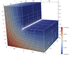
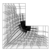
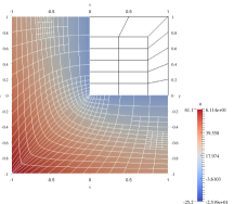
Due to the doubled control points in the corners of the L-shape domain (denoted by red and purple circles in Figure 18b), only the re-entrant corner and its counterpart on the other side are singular, i.e., the Jacobian of the geometry map in these two points is not regular. Since no integration points are placed in both corners, computational evaluation of the integrals remains valid. The downside of such a setting is that with the increase of refinement steps the cells near these corners become rather thin and lose shape-regularity. In addition, since on the functional level the requirements on the regularity of $\boldsymbol{y}$ are not fulfilled, the global error estimate has rather a heuristic character, therefore, we only consider its performance from error indication point of view.

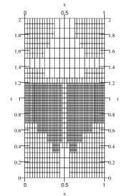
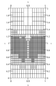
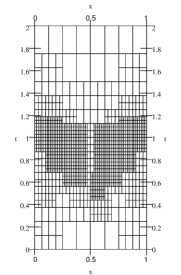
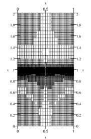
In Figure 19, we illustrate an evolution of adaptive meshes discretising physical domain (on LHS) and corresponding wireframes of meshes $\mathcal{K}_{h}$ (on RHS). L-shaped meshes (extended in time) on the right are illustrated from the point of view placed at the zero azimuth angle (located on the $O_{z}$-axis) in order to better see the nested THB-Splines. From both left and right columns, we can see that the refinement is localised in the area close to the singular point and no superfluous refinement is performed otherwise. Since the solution does not change in time drastically, the main refinement is concentrated in the area close to $(0,0)$. The efficiency of the studied error bounds is also confirmed in Table 14, which illustrates the decay of majorants and error identity w.r.t. refinement steps. Overall, $\overline{\rm M}^{\rm I}$ performs rather realistic, but even $\overline{\rm M}^{\rm I\!I}$ improves the first upper bound by approximately $1.5$ times. The e.o.c. (illustrated in the last column of Table 14) is recovered due to the adaptive procedure dictated by $\overline{\rm M}^{\rm I}$.

# ref.	$\|\nabla_{x}e\|_{Q}$	$\overline{\rm M}^{\rm I}$	$I_{\rm eff}(\overline{\rm M}^{\rm I\!I})$	$|\!|\!|e|\!|\!|_{s,h}$	$I_{\rm eff}(\overline{\rm M}^{\rm I}_{s,h})$	e.o.c. ($|\!|\!|e|\!|\!|_{s,h}$)
adaptive refinement, $\theta=0.4$
2	1.7985e-01	2.54	1.68	1.7993e-01	2.54	2.24
3	1.2011e-01	2.45	1.64	1.2020e-01	2.45	1.47
4	7.2490e-02	2.57	1.64	7.2494e-02	2.57	1.49
5	4.8546e-02	2.53	1.62	4.8550e-02	2.53	1.47

Table 14: Example 5. Efficiency of $\overline{\rm M}^{\rm I}$, $\overline{\rm M}^{\rm I\!I}$, and $\overline{\rm M}^{\rm I}_{s,h}$ for $u_{h}\in S^{2}_{h}$, $\boldsymbol{y}_{h}\in\oplus^{3}S_{h}^{3}$, and $w_{h}\in S^{3}_{h}$, w.r.t. adaptive refinement steps.

(a) ref. # 2:  ${\Omega}$ and ${\mathcal{K}}_{h}$

(b) ref. # 2:  ${\mathcal{K}}_{h}$, $O_{z}$-axis

(c) ref. # 4:  ${\Omega}$ and ${\mathcal{K}}_{h}$

(d) ref. # 4:  ${\mathcal{K}}_{h}$, $O_{z}$-axis

Figure 19: Example 5. Comparison of meshes on the physical domains w.r.t. adaptive refinement steps, criterion ${\mathds{M}}_{{\rm\bf BULK}}(0.4)$.

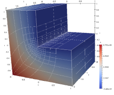
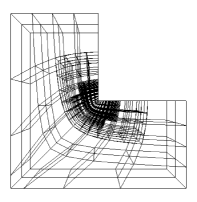
Next, we assume that $u(x,y,t)$ has a more complicated dependence on $t$ and set

$$\phi(t)=10\,(10\,t-\tfrac{1}{2})\,(t-1)\,(t-\tfrac{7}{4}).$$

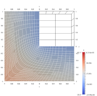
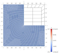
Then, the space-time approach of solving the problem provides mesh-refinement in space and time automatically. Figure 20 illustrates how $2$-dimensional spatial slices of the $3$-dimensional meshes involve w.r.t. time. Table 15 provides numerical evidence of how various error measures are estimated by $\overline{\rm M}^{\rm I}$, $\overline{\rm M}^{\rm I\!I}$, and $\overline{\rm M}^{\rm I}_{s,h}$.

# ref.	$\|\nabla_{x}e\|_{Q}$	$\overline{\rm M}^{\rm I}$	$I_{\rm eff}(\overline{\rm M}^{\rm I\!I})$	$|\!|\!|e|\!|\!|_{s,h}$	$I_{\rm eff}(\overline{\rm M}^{\rm I}_{s,h})$	e.o.c. ($|\!|\!|e|\!|\!|_{s,h}$)
adaptive refinement, $\theta=0.4$
2	9.3813e+00	1.66	1.44	1.0444e+01	1.49	4.52
3	5.7807e+00	1.74	1.20	5.9134e+00	1.70	1.61
4	1.8193e+00	2.92	1.36	1.8689e+00	2.85	2.51
5	1.0706e+00	2.44	1.40	1.0761e+00	2.43	1.43

Table 15: Example 5. Efficiency of $\overline{\rm M}^{\rm I}$, $\overline{\rm M}^{\rm I\!I}$, and $\overline{\rm M}^{\rm I}_{s,h}$ for $u_{h}\in S^{2}_{h}$, $\boldsymbol{y}_{h}\in\oplus^{3}S_{h}^{3}$, and $w_{h}\in S^{3}_{h}$, w.r.t. adaptive refinement steps.

(a) ${\mathcal{K}}_{h}$, $t=0$

(b) ${\mathcal{K}}_{h}$, $t=1$

(c) ${\mathcal{K}}_{h}$, $t=2$

Figure 20: Example 5. Comparison of meshes on the physical domains w.r.t. adaptive refinement steps, criterion ${\mathds{M}}_{{\rm\bf BULK}}(0.4)$.

6.6 Example 6 (solution with singularity w.r.t. $t$-coordinate)

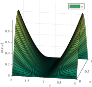
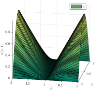
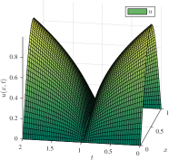
For the last example, we assume that the solution has singularity w.r.t. time coordinates, i.e., we consider

$$u(x,t)=\sin\pi x\,(1-t)^{\lambda}\in H^{\ell_{x},\ell_{t}}(Q),\ell_{x},\ell_{t}\geq 0,\quad(x,t)\in\overline{Q}=(0,1)\times(0,2),$$

where parameter $\lambda=\Big{\{}\tfrac{3}{2},1,\frac{1}{2}\Big{\}}$ (see Figure 21 with $u$ for different $\lambda$). The RHS $f(x,t)$ follows from substitution of $u$ into (1), and the Dirichlet boundary conditions are defined as $u_{D}=u$ on $\Sigma$.

(a) $\lambda=\tfrac{3}{2}$

(b) $\lambda=1$

(c) $\lambda=\tfrac{1}{2}$

Figure 21: Example 6. (a) Exact solution $u(x,t)=\sin\pi x\,(1-t)^{{}^{3}\!/_{2}}$. (b) Exact solution $u(x,t)=\sin\pi x\,|1-t|$.
(c) Exact solution $u(x,t)=\sin\pi x\,(1-t)^{{}^{1}\!/_{2}}$.

The solution $u(x,t)$ is smooth w.r.t. to spatial coordinates, and the regularity in time depends on parameter $\lambda$. In particular, $\ell_{t}$ must satisfy the following inequality $\lambda\geq\ell_{t}-\tfrac{d}{p}$, where $d$ is the dimension of $\Omega$, and $p$ is a degree of splines used for the approximation of $u$ (in the current case, $d=1$ and $p=2$). Then, we obtain the relation $\ell_{t}\leq\lambda+\tfrac{1}{2}$, and the expected convergence in the term $h^{{}^{1}\!/_{2}}\,\|\partial_{t}(u-u_{h})\|_{Q}$ is $(O(h^{\ell_{x}})+O(h^{\ell_{t}-1}))\cdot O(h^{{}^{1}\!/_{2}})$. These theoretical observations are confirmed by the numerical results presented in Table 16. The last column illustrates expected error order of convergence $O(h^{\ell_{t}-{}^{1}\!/_{2}})$. In particular, for the parameters $\lambda=\big{\{}\frac{1}{2},1,\tfrac{3}{2}\big{\}}$, we expect $\ell_{t}\leq\big{\{}2,\tfrac{3}{2},1\big{\}}$, which provides approximated e.o.c. ${O(h^{{}^{3}\!/_{2}})}$, ${O(h^{1})}$, and ${O(h^{{}^{1}\!/_{2}})}$, respectively. Table 16 also provides the error’s and estimates’ decay in the case of adaptive refinement. The last column confirmes an improved e.o.c.

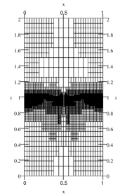
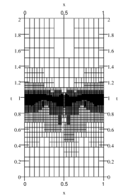
Figure 22 presents meshes obtained on the adaptive refinement steps 5 and 6 and reconfirms that functional error estimates detect the local singularities rather well. We see that for $\lambda=\tfrac{1}{2}$, the singularity at $t=1$ is captured and very well represented by the adaptive mesh. Moreover, for $t>1$, where the solution is smooth, the mesh is not over-refined.

# ref.	$\|\nabla_{x}e\|_{Q}$	$I_{\rm eff}(\overline{\rm M}^{\rm I\!I})$	$|\!|\!|e|\!|\!|_{s,h}$	$I_{\rm eff}(\overline{\rm M}^{\rm I}_{s,h})$	$|\!|\!|e|\!|\!|_{\mathcal{L}}$	$I_{\rm eff}({{\rm E\!\!\!Id}})$	e.o.c. ($|\!|\!|e|\!|\!|_{s,h}$)
$\lambda=\tfrac{3}{2}$
uniform refinement							expected ${O\big{(}h^{{}^{3}\!/_{2}}\big{)}}$
4	3.7789e-03	1.13	8.6838e-03	9.05	2.8189e-01	1.00	2.05
5	9.5349e-04	1.52	2.8772e-03	9.73	1.4075e-01	1.00	1.74
6	2.4077e-04	2.28	9.9310e-04	10.14	7.0358e-02	1.00	1.60
adaptive refinement, $\theta=0.4$							improved e.o.c.
3	1.7464e-02	1.00	1.7464e-02	2.10	5.6998e-01	1.00	2.50
4	5.6537e-03	1.43	5.6537e-03	3.47	2.8936e-01	1.00	2.08
6	1.7847e-03	1.48	1.7847e-03	3.43	1.6984e-01	1.00	2.32
7	7.0591e-04	1.65	7.0591e-04	4.00	1.3543e-01	1.00	2.16
$\lambda=1$
uniform refinement							expected ${O(h)}$
4	1.6706e-02	1.15	5.0754e-02	2.89	3.7940e-01	1.00	1.32
5	5.9650e-03	1.71	2.4711e-02	2.88	2.1176e-01	1.00	1.13
6	2.1355e-03	2.86	1.2256e-02	3.31	1.2604e-01	1.00	1.06
adaptive refinement, $\theta=0.4$							improved e.o.c.
3	5.8230e-02	1.06	5.8230e-02	2.39	7.4729e-01	0.99	1.73
4	2.7175e-02	1.42	2.7175e-02	3.75	5.4388e-01	1.00	1.64
5	2.5989e-02	1.35	2.5989e-02	3.27	5.8875e-01	1.00	0.10
6	1.2191e-02	1.69	1.2191e-02	4.56	5.1917e-01	1.00	1.85
$\lambda=\tfrac{1}{2}$
uniform refinement							expected ${O\big{(}h^{{}^{1}\!/_{2}}\big{)}}$
4	5.3129e-02	1.40	2.0530e-01	2.00	9.0200e-01	1.00	0.67
5	2.6997e-02	2.16	1.4296e-01	2.29	8.2282e-01	1.00	0.57
6	1.3712e-02	3.67	1.0061e-01	2.96	8.0464e-01	1.00	0.53
adaptive refinement, $\theta=0.4$							improved e.o.c.
5	5.8991e-02	2.05	5.8991e-02	6.13	2.2131e+00	1.00	0.97
6	3.8622e-02	3.01	3.8622e-02	9.93	2.3304e+00	1.00	1.11
7	2.5883e-02	3.88	2.5883e-02	14.66	2.6588e+00	1.00	1.15
8	2.0120e-02	4.24	2.0120e-02	16.98	3.4281e+00	1.00	0.70

Table 16: Example 6. Efficiency of $\overline{\rm M}^{\rm I\!I}$, $\overline{\rm M}^{\rm I}_{s,h}$, and ${{\rm E\!\!\!Id}}$ for $u_{h}\in S^{2}_{h}$, $\boldsymbol{y}_{h}\in\oplus^{3}S_{h}^{3}$, and $w_{h}\in S^{3}_{h}$, w.r.t. uniform refinement and adaptive refinement steps.

(a) ref. # 4:  ${\mathcal{K}}_{h}$, $\lambda=\tfrac{3}{2}$

(b) ref. # 4:  ${\mathcal{K}}_{h}$, $\lambda=1$

(c) ref. # 4:  ${\mathcal{K}}_{h}$, $\lambda=\tfrac{1}{2}$

(d) ref. # 6:  ${\mathcal{K}}_{h}$, $\lambda=\tfrac{3}{2}$

(e) ref. # 6:  ${\mathcal{K}}_{h}$, $\lambda=1$

(f) ref. # 6:  ${\mathcal{K}}_{h}$, $\lambda=\tfrac{1}{2}$

Figure 22: Example 6. Comparison of meshes on the physical and parametric domains w.r.t. adaptive refinement steps, criterion ${\mathds{M}}_{{\rm\bf BULK}}(0.4)$.

7 Conclusions

In the paper, we derived reliable space-time IgA schemes for parabolic initial-boundary value problems. In particular, we deduced new functional-type a posteriori error estimates and showed their efficient implementation in space-time IgA. Since the derivation is based on purely functional arguments, the estimates are valid for any approximation from the admissible (energy) class. They imply a posteriori error estimates for mesh-dependent norms associated with stabilised space-time IgA schemes. We also proposed an efficient technique for minimising the majorant leading to extremely accurate guaranteed upper bounds of the error norm with efficiency indices close to 1. Since this upper bound is nothing but the sum of the local contributions, these local contributions were be used as error indicators for mesh refinement. Mesh refinement in IgA is more involved than in the finite element method. We used THB-Splines for mesh refinement in our fully unstructured space-time adaptive IgA scheme. Finally, we illustrated the reliability and efficiency of the presented a posterior error estimates for IgA solutions to several examples exhibiting different features (defined on the domains with non-trivial shape, having solutions that possess singularity w.r.t. space and time variables). We also reported about the cost of computing the upper bound. In all our examples, this was only a small portion of the cost for computing the IgA solution. Last but not least, the numerical examples showed that the space-time THB-spline-based adaptive procedure works very efficiently.

Acknowledgments The research is supported by the Austrian Science Fund (FWF) through the NFN S117-03 project. The implementation was carried out using the open-source C++ library G+Smo [22].

References

- [1] I. Anjam and D. Pauly. An elementary method of deriving a posteriori error equalities and estimates for linear partial differential equations. Computers and Mathematics with Applications (CMAM), 2017. accepted for publication, also available as arxiv-report with a number arxiv:math.NA:1612.01411.
- [2] N. S. Bakhvalov. On the convergence of a relaxation method with natural constraints on the elliptic operator. USSR Comp. Math. Math. Phis., 6(5):101–135, 1966.
- [3] Y. Bazilevs, L. Beirão da Veiga, J. A. Cottrell, T. J. R. Hughes, and G. Sangalli. Isogeometric analysis: approximation, stability and error estimates for -refined meshes. Math. Models Methods Appl. Sci., 16(7):1031–1090, 2006.
- [4] A. Brandt. Multi-level adaptive techniques (mlat) for fast numerical solution to boundary value problems. In Lecture Notes in Physics, 1973. Proc. 3rd Internat. Conf. on Numerical Methods in Fluid Mechanics, Paris, 1972.
- [5] A. Buffa and C. Giannelli. Adaptive isogeometric methods with hierarchical splines: error estimator and convergence. Mathematical Models and Methods in Applied Sciences, 26(1):1–25, 2016.
- [6] R. Dautray and J. L. Lions. Mathematical Analysis and Numerical Methods for Science and Technology. Volume 5. Evolution Problems I. Springer, Heidelberg, Germany, 2000.
- [7] R. Dautray and J. L. Lions. Mathematical Analysis and Numerical Methods for Science and Technology. Volume 6. Evolution Problems II. Springer, Heidelberg, Germany, 2000.
- [8] L. Dedè and H. A. F. A. Santos. B-spline goal-oriented error estimators for geometrically nonlinear rods. Comput. Mech., 49(1):35–52, 2012.
- [9] M. R. Dörfel, B. Jüttler, and B. Simeon. Adaptive isogeometric analysis by local -refinement with T-splines. Comput. Methods Appl. Mech. Engrg., 199(5-8):264–275, 2010.
- [10] W. Dörfler. A convergent adaptive algorithm for Poisson’s equation. SIAM J. Numer. Anal., 33(3):1106–1124, 1996.
- [11] K. Friedrichs. On certain inequalities and characteristic value problems for analytic functions and for functions of two variables. Trans. Amer. Math. Soc., 41(3):321–364, 1937.
- [12] M. Gander. 50 years of time parallel time integration. In Multiple Shooting and Time Domain Decomposition, volume 16, pages 69–114. Springer-Verlag, Berlin, 2015. Theory, algorithm, and applications.
- [13] M. Gander and M. Neumüller. Analysis of a new space-time parallel multigrid algorithm for parabolic problems. SIAM J. Sci. Comput., 38(4):A2173–A2208, 2016.
- [14] G. Gantner, D. Haberlik, and D. Praetorius. Adaptive igafem with optimal convergence rates: Hierarchical B-splines. Technical Report arXiv:1701.07764v3 [math.NA], arxiv:math.NA, 2017.
- [15] Gaël Guennebaud, Benoît Jacob, et al. Eigen v3. http://eigen.tuxfamily.org, 2010.
- [16] W. Hackbusch. Multi-Grid Methods and Applications. Springer, Berlin, 1985.
- [17] P. Hansbo. Space-time oriented streamline diffusion methods for nonlinear conservation laws in one dimension. Comm. Numer. Meth. Eng., 10(3):203–215, 1994.
- [18] B. Holm and S. Matculevich. Fully reliable error control for evolutionary problems. Computers and Mathematics with Applications (CAMWA), 2017. accepted for publication, also available as arxiv-report with a number cs.NA:1705.08614.
- [19] K.A. Johannessen. An adaptive isogeometric finite element analysis. Technical report, Master’s thesis, Norwegian University of Science and Technology, 2009.
- [20] C. Johnson. Numerical solution of partial differential equations by the finite element method. Dover Publications, Inc., Mineola, NY, 1987.
- [21] C. Johnson and J. Saranen. Streamline diffusion methods for the incompressible Euler and Navier-Stokes equations. Math. Comp., 47(175):1–18, 1986.
- [22] B Jüttler, Hofreither C., C. Hofer, A. Mantzaflaris, S. Matculevich, F. Scholz, Sogn J., Takacs A., and others (see website). G+smo (geometry plus simulation modules) v0.8.1. http://gs.jku.at/gismo, 2015.
- [23] S. K. Kleiss and S. K. Tomar. Guaranteed and sharp a posteriori error estimates in isogeometric analysis. Comput. Math. Appl., 70(3):167–190, 2015.
- [24] M. Kumar, T. Kvamsdal, and K. A. Johannessen. Simple a posteriori error estimators in adaptive isogeometric analysis. Comput. Math. Appl., 70(7):1555–1582, 2015.
- [25] G. Kuru. Goal-adaptive isogeometric analysis with hierarchical splines. Technical report, Master’s thesis, Mechanical Engineering, Eindhoven University of Technology, 2013.
- [26] G. Kuru, C. V. Verhoosel, K. G. van der Zee, and E. H. van Brummelen. Goal-adaptive isogeometric analysis with hierarchical splines. Comput. Methods Appl. Mech. Engrg., 270:270–292, 2014.
- [27] O. A. Ladyzhenskaya. On solvability of classical boundary value problems for equations of parabolic and hyperbolic types. Dokl. Akad. Nauk SSSR, 97(3):395–398, 1954.
- [28] O. A. Ladyzhenskaya. The boundary value problems of mathematical physics. Springer, New York, 1985.
- [29] U. Langer, S. Matculevich, and S. Repin. Functional type error control for stabilised space-time iga approximations to parabolic problems. In I. Lirkov and S. Margenov, editors, Large-Scale Scientific Computing (LSSC 2017), Lecture Notes in Computer Science (LNCS), pages 57–66. Springer-Verlag, 2017. accepted for publication, also available as RICAM Report 2017-14 at https://www.ricam.oeaw.ac.at/files/reports/17/rep17-14.pdf.
- [30] U. Langer, S. Moore, and M. Neumüller. Space-time isogeometric analysis of parabolic evolution equations. Comput. Methods Appl. Mech. Engrg., 306:342–363, 2016.
- [31] O. Mali, P. Neittaanmäki, and S. Repin. Accuracy verification methods, volume 32 of Computational Methods in Applied Sciences. Springer, Dordrecht, 2014.
- [32] S. Matculevich, P. Neittaanmäki, and S. Repin. A posteriori error estimates for time-dependent reaction-diffusion problems based on the Payne–Weinberger inequality. AIMS, 35(6):2659–2677, 2015.
- [33] S. Matculevich and S. Repin. Computable estimates of the distance to the exact solution of the evolutionary reaction-diffusion equation. Appl. Math. and Comput., 247:329–347, 2014.
- [34] S. Repin. A posteriori estimates for partial differential equations, volume 4 of Radon Series on Computational and Applied Mathematics. Walter de Gruyter GmbH & Co. KG, Berlin, 2008.
- [35] S. Repin, S. Sauter, and A. Smolianski. A posteriori error estimation for the Dirichlet problem with account of the error in the approximation of boundary conditions. Computing, 70(3):205–233, 2003.
- [36] S. I. Repin. Estimates of deviations from exact solutions of initial-boundary value problem for the heat equation. Rend. Mat. Acc. Lincei, 13(9):121–133, 2002.
- [37] S.I. Repin. A posteriori error estimation for nonlinear variational problems by duality theory. Zapiski Nauchnych Seminarov POMIs, 243:201–214,, 1997.
- [38] S.I. Repin. A posteriori error estimates for approximate solutions to variational problems with strongly convex functionals. Journal of Mathematical Sciences, 97:4311–4328, 1999.
- [39] A. Tagliabue, L. Dedè, and A. Quarteroni. Isogeometric analysis and error estimates for high order partial differential equations in fluid dynamics. Comput. & Fluids, 102:277–303, 2014.
- [40] K. G. van der Zee and C. V. Verhoosel. Isogeometric analysis-based goal-oriented error estimation for free-boundary problems. Finite Elem. Anal. Des., 47(6):600–609, 2011.
- [41] A.-V. Vuong, C. Giannelli, B. Jüttler, and B. Simeon. A hierarchical approach to adaptive local refinement in isogeometric analysis. Comput. Methods Appl. Mech. Engrg., 200(49-52):3554–3567, 2011.
- [42] P. Wang, J. Xu, J. Deng, and F. Chen. Adaptive isogeometric analysis using rational pht-splines. Computer-Aided Design, 43(11):1438–1448, 2011.
- [43] E. Zeidler. Nonlinear functional analysis and its applications. II/A. Springer-Verlag, New York, 1990.