Bulk-edge correspondence and topological phases in periodically driven spin-orbit coupled materials in the low frequency limit

Abstract

We study the topological phase transitions induced in spin-orbit coupled materials with buckling like silicene, germanene, stanene, etc, by circularly polarised light, beyond the high frequency regime, and unearth many additional topological phases. We also study the robustness of these phases in the presence of uniform disorder. These phases are characterised by the spin-resolved topological invariants, $C_{0}^{\uparrow}$, $C_{0}^{\downarrow}$, $C_{\pi}^{\uparrow}$ and $C_{\pi}^{\downarrow}$, which specify the spin-resolved edge states traversing the gaps at zero quasi-energy and the Floquet zone boundaries respectively. We show that for each phase boundary, and independently for each spin sector, the gap closure in the Brillouin zone occurs at a high symmetry point.

I Introduction

Dynamical control of topological phases is one of the most intensely researched topics in recent timesOka2009 ; Kitagawa2010 ; Gu2011 ; Lindner2011 ; Jiang2011 ; Calvo2011 ; Dora2012 ; Kundu2013 ; Kundu2014 ; Ezawa2013 . Proposals have involved periodic driving in semiconductor systemsLindner2011 , cold atom (or optical lattice) systemsJiang2011 , grapheneOka2009 ; Kitagawa2010 ; Gu2011 ; Kundu2014 and systems with spin-orbit coupling like siliceneEzawa2013 , with a variety of analytical and numerical methods. Apart from band-structure control of a system by renormalization of its dynamical parameters via a periodic drive, novel non-trivial topological phases, which do not have any analog in static systems, have been explored, theoretically  Rudner2013 ; Platero2013 ; Platero2014 ; Carpentier2014 ; Sentef2015 ; Fistul2015 as well as in experimental photonic systemsMaczewsky2017 ; Mukherjee2017expt .

Silicene Ezawa2011a , and other spin-orbit coupled Konschuh2010 materials like germanene, stanene, etc are recently synthesized materials which have shot into prominence because their buckled nature allows them to be tuned by an electric field through a transition between a band insulator and a topological insulator Kane2005 ; Hasan2010 ; Qi2011 . This tunability, and in particular, the experimental realisation Tao2015 of silicene-based transistors has led to extensive work Linder2014 ; Rachel2014 ; Saxena2015 ; Paul2016 ; Li2016 ; Sarkar2016 on the interplay of topology and transport in these materials.

More recently, the question of whether topological phases can be controlled in irradiated silicene and similar materials has been studied. Although these materials are time-reversal invariant, in the presence of circularly polarised light, the system breaks time-reversal symmetry and the Chern number classification is integer and not $Z_{2}$ invariant. Ezawa Ezawa2013 showed that at high frequencies and for small amplitudes of driving, new phases in silicene such as quantum Hall insulator, spin-polarised quantum Hall insulator and spin and spin-valley polarised metals can be realised. Further, it was shown Mohan2016 that many more topological phases could be realised by performing a systematic Brillouin-Wigner (BW) expansion of the Hamiltonian to second order in the inverse of the frequency, not only in silicene, but in other spin-orbit coupled materials. But, as was discussed also in earlier references Mohan2016 ; Mikami2016 , the BW expansion breaks down when the frequency $\omega$ becomes smaller than the band-width of the effective Hamiltonian. The real constraint on the applicability of the BW expansion is a combined bound on both $\omega$ and the amplitude of driving and in fact, the validity of BW increases, even for lower frequencies when the amplitude increases. However, the physical reason for the breakdown of the earlier studies at low frequencies is because, at frequencies comparable to the band-width, it is no longer possible to neglect the topology of the quasienergy space, which forms a periodic structure with the single valuedness of the eigenfunction requiring the quasienergies to be within a “Floquet zone”. Low frequency driving can lead to crossings between the bottom of one Floquet band and the top of the next Floquet band. These crossings are neglected in the BW expansion and hence, the study of the driving at low frequencies requires a new formalism which goes beyond the effective static approximation of a dynamical Hamiltonian.

To characterize the topological nature of these system that would satisfy the edge-bulk correspondence, one needs to have access to the full time-dependent bulk evolution operator $U(t)$, evaluated for all intermediate times within the driving period Rudner2013 . The invariants thus computed predict the complete Floquet edge-state spectrum. Similar $Z_{2}$ valued indices for periodically driven time-reversal invariant two dimensional indices have also been found Carpentier2014 . For a two band model with the Fermi energy at zero quasi-energy, it was shown that the gaps at zero quasi-energy and at the zone boundary $\omega/2$ gave rise to winding numbers $C_{0}$ and $C_{\pi}$, whose difference gave the Chern number of the band. This formalism has been used to demonstrate the bulk-boundary correspondence in graphene  Kundu2014 ; graphene .

However, most of the studies have focused on graphene both in the high and low frequency regimes and silicene-like materials have not been fully explored when they are exposed to low frequency radiation. In this paper, we study the photo induced topological phase diagram in these materials by computing the topological invariant for both up and down spin. We also look for the gap closing points in the Brillouin zone and find that it always occur at the high symmetry points. Further, we compute $C_{0}$ and $C_{\pi}$ by counting the number of edge states at the right and left edges of the sample and verify the bulk-boundary correspondence as illustrated earlier in graphene  Kundu2014 ; graphene . Although the question of whether these topological phases obtained in the low frequency regime are stable or not, requires detailed analysis to answer definitively, here we just address the behaviour of a few phases against uniform disorder by computing the real space Chern number using the coupling matrix approach prescribed in  coupling . A full analysis is left for future studies. We further note that our study can also be extended to two dimensional optical lattices where one can artificially synthesise an effective spin-orbit coupling by a combination of microwave driving and lattice shaking  optical , and also to ultra cold atoms  coldatom , in both bosonic  bosonic_1 ; bosonic_2 and fermionic systems  fermionic1 ; fermionic2 where the Raman coupling has been shown to give rise to an effective spin-orbit interaction.

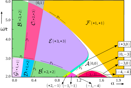
Figure 1: The phase diagram for the model Hamiltonian in Eq. 1 as we vary the amplitude $\alpha$ and the drive frequency $\omega$, with the external electric field fixed at $lE_{z}=0.08t$ and spin-orbit coupling, $\lambda_{SO}$ at 0.05t. Each phase is characterized by the spin resolved quantum numbers ($C_{\uparrow}$, $C_{\downarrow}$). We label the phases by calligraphic letters. The dotted lines $P_{i}$ indicate the topological phase boundaries, inferred from the gap closing in momentum space, shown only for the $\uparrow$ spin sector.

II Computation of the dynamical band structure

We start with two dimensional Dirac systems which are buckled due to the large ionic radius of the silicon atoms and consequently have a non-coplanar structure unlike graphene. These materials can be described by a four-band tight binding model in a hexagonal lattice given by

$$H=-t\sum_{\langle i,j\rangle,\sigma}c_{i\sigma}^{\dagger}c_{j\sigma}+\frac{i\lambda}{3\sqrt{3}}\sum_{\langle\langle i,j\rangle\rangle,\sigma}\sigma\nu_{i,j}c_{i\sigma}^{\dagger}c_{j\sigma}$$

$$+lE_{z}\sum_{i\sigma}\xi_{i}c_{i\sigma}^{\dagger}c_{i\sigma}~{}.$$ (1)

Here, the first term is the kinetic term where $t$ is the hopping parameter. The second term represents the spin-orbit coupling term where the value of $\lambda$ depends on the material and $\nu_{i,j}=\pm 1$ depending on whether the next-nearest neighbour hopping is clock-wise or anti-clock-wise. The last term represents the staggered sub-lattice potential due to the buckling. When a beam of circularly polarised light is incident on the sheet, the corresponding electro-magnetic potential ${\bf A}=(A_{0}\cos(\omega\tau),A_{0}\sin(\omega\tau),0)$ is introduced into the Hamiltonian using Peierls substitution. $\omega$ is the frequency of light and $A_{0}$ is its amplitude. In the Fourier transformed space, this is written as

$$H(\tau)=\left(\begin{array}[]{cccc}lE_{z}-\delta_{\lambda}&\delta_{t}&0&0\\ \delta_{t}^{*}&-lE_{z}+\delta_{\lambda}&0&0\\ 0&0&lE_{z}+\delta_{\lambda}&\delta_{t}\\ 0&0&\delta_{t}^{*}&-lE_{z}-\delta_{\lambda}\end{array}\right)$$ (6)

where

$$\delta_{\lambda}(\tau)=\frac{2\lambda}{3\sqrt{3}}\left[\sqrt{3}a_{0}\sin{\tilde{k}_{x}}-\sin\left(\frac{\sqrt{3}a_{0}}{2}{\tilde{k}_{x}}+\frac{3a_{0}}{2}{\tilde{k}_{y}}\right)\right.$$

$$\left.-\sin\left(\frac{\sqrt{3}a_{0}}{2}{\tilde{k}_{x}}-\frac{3a_{0}}{2}{\tilde{k}_{y}}\right)\right]$$ (7)

with ${\tilde{k}_{x}}=k_{x}+A\cos\omega\tau$ and ${\tilde{k}_{y}}=k_{y}+A\sin\omega\tau$ and

$$\delta_{t}(\tau) =t\left[{\rm exp}(-i\alpha\sin\omega\tau)\right.$$

$$\left.+T_{+}{\rm exp}\frac{i\alpha(\sqrt{3}\cos\omega\tau+\sin\omega\tau)}{2}\right.$$

$$\left.+T_{-}{\rm exp}\frac{i\alpha(-\sqrt{3}\cos\omega\tau+\sin\omega\tau)}{2}\right]$$ (8)

with $T_{\pm}={\rm exp}(ia_{0}(\pm\sqrt{3}k_{x}+{3k_{y}}/2))$. Here, we have defined $\alpha=Aa_{0}$, where $a_{0}$ is the lattice constant.

For the bulk system, the vector potential and hence the Hamiltonian is periodic in both the $x$ and $y$ directions. This implies that we can rewrite the Hamiltonian in terms of a Floquet eigenvalue problem with the Hamiltonian given by

$$H_{F}=-i\frac{\partial}{\partial\tau}+H(\tau),$$ (9)

the eigen functions given by

$$\psi_{{\bf k},b}(x,y,\tau)=u_{b}(k_{x},k_{y},\tau)e^{i{\bf r}\cdot{\bf k}-i\epsilon_{b}\tau}$$ (10)

with $u_{b}(k_{x},k_{y},\tau)=u_{b}(k_{x},k_{y},\tau+2\pi/\omega)$, and where $\epsilon_{b}$ are the quasienergies or the eigenvalues of $H_{F}$. The Hamiltonian can now be solved numerically as a function of the amplitude $A_{0}$, frequency $\omega$ and the sub-lattice potential $E_{z}$, both for the quasienergy eigenvalues and for the wave-functions.

At high frequencies, $\omega$ constitutes a large gap between unperturbed subspaces, and the extended Floquet Hilbert space splits into decoupled subspaces with different photon numbers. Since the perturbation scale of the Hamiltonian, which is the band-width $t$, is much smaller than $\omega$, one can use systematic perturbation theory to include virtual processes of emitting and absorbing photons, and upto a given order in perturbation theory, one can obtain an effectively static Hamiltonian as shown in Ref. Mohan2016, . The Chern numbers for the model can then be computed by integrating the Berry curvature over the whole Brillouin zone Hatsugai_2005 using the eigenvectors of the effective Hamiltonian. However it is expected that such an expansion in $1/\omega$ would fail to predict the correct Chern numbers once the frequency of the drive, $\omega$, becomes comparable to the bandwidth. This is the part of the phase diagram that we shall complete in this paper.

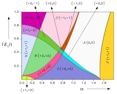
Figure 2: The phase diagram as a function of the amplitude $\alpha$ and the external electric field $lE_{z}$. A low frequency drive is chosen ($\omega=3.0t$) since we wish to study the system in the low frequency limit. All the phases are the same as those found in Fig.1 except for three new phases - $\mathcal{H}$, $\mathcal{I}$ and $\mathcal{J}$. The labelling of the phases follows the same convention as in Fig. 1.

II.1 The phase diagram of the Floquet Hamiltonian

As the frequency of the drive becomes comparable to the effective bandwidth of the system, it is essential to now consider the complete nature of the quasi-energy bands in the computation of the topological invariants of the system. As was mentioned in the introduction, the quasi-energy bands (of the two band system) are now identified with two topological invariants, $C_{0}$ and $C_{\pi}$ and the net Chern number of a band is given by $C=C_{0}-C_{\pi}$ (independently for each of the spins).

The Fourier-transformed time-dependent Hamiltonian (Eq. 2) is block-diagonal in the spin space. For either the $\uparrow$ or the $\downarrow$ spin, it is a 2 $\times$ 2 Hermitian matrix which encodes the bulk properties of the system. The time evolution operator at stroboscopic times can then be written as

$$U(\textbf{k},2\pi/\omega)=\mathcal{T}e^{-i\int_{0}^{2\pi/\omega}H(\textbf{k},\tau)d\tau}.$$ (11)

and the Floquet states $u_{b}(k_{x},k_{y},0)$ are the eigenstates of this operator. The Chern number of each Floquet band is then defined by integrating the Berry curvature of the Floquet states over the whole Brillouin zone -

$$C=\frac{1}{2\pi}\int_{BZ}dk_{x}dk_{y}(\nabla\times\mathcal{A}_{\text{lower}}(\mathbf{k})),$$ (12)

where $\mathcal{A}_{\text{lower}}$ is the Berry connection in terms of Floquet states of the quasi-energy band with quasienergy lying between ($-\omega/2$, 0). We numerically compute the Chern numbers of the lower band (of both $\uparrow$ and $\downarrow$ spins) following the work by Fukui et al Hatsugai_2005 .

When the parameter ranges are such that a high frequency approximation would be valid, the Chern number computed using the effective static Hamiltonian would exactly match the one obtained by considering the Floquet states. In this sense, the following phase diagram that we present complements what has been obtained earlier in Ref. Mohan2016, , and completely specifies the topological phases of the system for all parameter regimes.

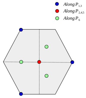
Figure 3: Gap closing points in the Brillouin zone along the $P_{i}\,\,(i=1\dots 6)$ phase boundaries (drawn in Fig.1) as described in the caption of Fig.1.

The phase diagrams for both the up spin and the down spin bands are presented in Figs. 1 and 2. In Fig. 1, we show the Chern number of the lower quasienergy band as a function of the amplitude of the drive versus the frequency, whereas in Fig. 2 we show it as a function of the amplitude of the drive versus the sub-lattice potential. For lower frequencies, many different phases appear and appear to follow a fractal structure, as was seen for graphene in Ref.Mikami2016 . But as such phases are not expected to be protected by a large enough band-gap, we have only shown phases which are ‘large enough’ (occupy enough area in the phase diagram) and we have ignored tinier phases. As $\alpha\rightarrow 2$ and $\omega\rightarrow 6$, these phases smoothly go over to the high frequency phases in Ref. Mohan2016, . We have also chosen to name only those phases that are large enough to be possible stable phases in calligraphic letters as $\mathcal{A},\mathcal{B}\dots\mathcal{J}$, with $\mathcal{A},\mathcal{B},\mathcal{C},\mathcal{E},\mathcal{F}$ being present in both Figs. 1 and 2, and $\mathcal{B^{\prime}},\mathcal{D},\mathcal{G}$ in Fig.1 and $\mathcal{H},\mathcal{I},\mathcal{J}$ in Fig. 2. Note that there are two phases $\mathcal{B}$ and $\mathcal{B^{\prime}}$ which have identical values of the Chern numbers for both the $\uparrow$ spin band and the $\downarrow$ spin band. Nevertheless, they are two distinct phases since they occur for different values of $\omega$ and $\alpha$ and are not continuously connected to each other and they could have different edge state structures. Note also the existence of a phase $\mathcal{A}$ which has zero Chern numbers for both spin $\uparrow$ and spin $\downarrow$ electrons. We will see later in the next section, that this is a topological phase and has edge states despite having zero Chern numbers.

The lines that separate the phases are when the gap closes and the gap closing typically occurs at the high symmetry points of the Brillouin zone as shown in Fig. 3. For the lines $P_{2},P_{4}$ and $P_{5}$, the gap closes at the $\Gamma$ point whereas for the $P_{1}$ and $P_{3}$ lines, it closes at the $K$ point and for the $P_{6}$ line, the closure happens at the half-way point between the $\Gamma$ point and the $K$ point. Note that we have concentrated on the spin $\uparrow$ bands and hence have lines separating region $\mathcal{C}$ from $\mathcal{E}$, which have different Chern numbers for $\uparrow$ spin, but no line separating regions $\mathcal{C}$ from $\mathcal{B}$, which have the same Chern number for $\uparrow$ spin. A similar analysis can be done for the $\downarrow$ spin case.

We note that the Chern number changes by $\pm 2$ at the $P_{5}$ crossing, which essentially implies a quadratic touching of the bands. This is similar to the transition explained in Ref. Kundu2014, where the Hamiltonian for the first $\Gamma$ point transition at the Floquet zone boundary was obtained perturbatively, and was shown to lead to a Chern number change of $\pm 2$. This can only happen at the spherically symmetric $\Gamma$ point. Along $P_{1},P_{2},P_{3}$ and $P_{4}$, the change in the Chern number is $\pm 1$ and the band touching happens at the $\Gamma$ or $K$ points. Along $P_{6}$, however, the change in the Chern number is $\pm 3$. This can happen at 3 points in the Brillouin zone, symmetric around the $\Gamma$ point as shown in Fig. 3. We have also checked that a change of the chirality of the circularly polarized light, besides changing signs of all the Chern numbers also breaks inversion symmetry with respect to the gap closing diagram in Fig. 3. The blue points are at $K^{\prime}$ instead of $K$ points and the green points are placed so as to complete the smaller hexagon.

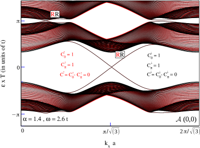
Figure 4: The quasi-energy band structure of a zigzag nanoribbon of the periodically driven spin-orbit coupled system for phase $\mathcal{A}$. Both spin sectors, $\uparrow$ and $\downarrow$ (shown in red and black respectively) possesses one pair of chiral edge states both at zero quasi energy and Floquet zone boundary. We also label the chirality of the left edge state at the two inequivalent gaps by R or L depending on whether the state is right-moving or left-moving. The system is finite in the $y$-direction while the $x$-direction is periodic.

However, the computation of the Chern number does not specify the $C_{0}$ and $C_{\pi}$ invariants individually. As the bulk-boundary correspondence in our system comes from these invariants, to discover these two indices, we need to consider the edge-state structure in a system with edges - $e.g$., a ribbon geometry. This is what we shall discuss in the following section.

Table 1: Spin-resolved topological quantum numbers and the edge states for phases in Figs.1, 2

. Phases    ($C^{\uparrow},C^{\downarrow}$)    $C_{0}^{\uparrow}$    $C_{\pi}^{\uparrow}$    $C_{0}^{\downarrow}$     $C_{\pi}^{\downarrow}$ $\mathcal{A}$ (0,0) 1 1 1 1 $\mathcal{B},\mathcal{B^{\prime}}$ (+2,+2) 0 $-2$ 0 $-2$ $\mathcal{C}$ (+2,+3) 0 $-2$ 1 $-2$ $\mathcal{D}$ (+1,+2) $-1$ $-2$ 0 $-2$ $\mathcal{E}$ (+3,+3) 1 $-2$ 1 $-2$ $\mathcal{F}$ (+1,+1) 1 0 1 0 $\mathcal{G}$ (+1,+1) $-1$ $-2$ $-1$ $-2$ $\mathcal{H}$ (+1,+1) 0 $-1$ 0 $-1$ $\mathcal{I}$ ($-2,-2$) 0 2 0 2 $\mathcal{J}$ ($-1,-1$) 0 1 0 1

II.2 Edge states in a ribbon geometry

In this section, we study the quasi-energy band-structure of the model in an infinite zigzag nanoribbon geometry, with a finite width. We identify the four integers $C_{0}^{\uparrow},C_{0}^{\downarrow},C_{\pi}^{\uparrow},C_{\pi}^{\downarrow}$ (defined later) that characterize Floquet topological insulators in our model, in each of the phases in Fig. 1 and 2, by choosing appropriate values of $\omega$, $\alpha$ and $lE_{z}$. A representative diagram for the phase $\mathcal{A}$ has been shown in Fig. 4 and the remaining diagrams have been relegated to the appendix. The spectrum has been shown slightly beyond the ‘first Floquet-Brillouin zone’, $-\omega/2<\epsilon_{b}<\omega/2$, so that the edge states at the zone boundaries are clearly visible.

The first point that we note is the gaps and the edge states at the zone boundaries (at $\epsilon_{b}=\omega/2\equiv-\omega/2$). In the high frequency regime studied earlier, we had restricted ourselves to frequencies below the zone boundaries (i.e, at $\epsilon=\pm\omega/2$), and hence the edge states at the zone boundary do not appear. However, in this work, our main focus is on the low frequency regime, and one of our aims is to explicitly check that the Chern number of the band is given by the difference between the number of chiral edge states above and below the band. How do we count the number of chiral edge states? As shown in Ref. [Rudner2013, ], the number of edge modes are related to the winding number of the Floquet operator. Unlike the Chern number of a band, which depends only on the stroboscopic dynamics of the Floquet operator, the winding number has information about the circulation direction, which gets related to the direction of propagation of the edge states. In a Floquet system, the chirality at a given edge depends on details of the driving and can be either positive or negative, independent of the chirality of the driving forcePlatero2014 . The chirality of the driving force only provides the required time-reversal breaking. However, at low frequencies, there is no direct relation between the chirality of the drive and the chirality of the edge states, since the drive can lead to multiple gap closings and openings with multiple edge states. Hence, the edge state chirality needs to be explicitly computed for each phase.

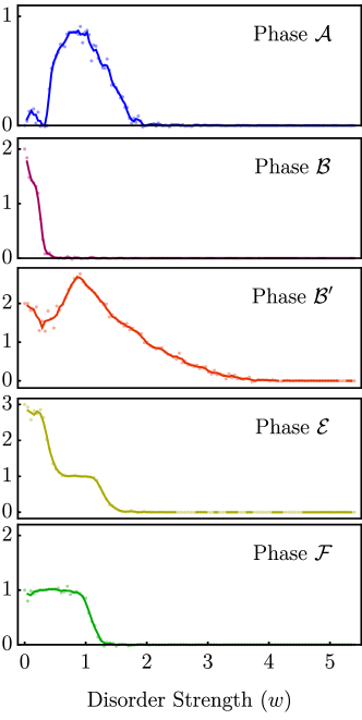
Figure 5: The disorder averaged real-space ‘Chern numbers’ for the $\uparrow$ spin sector is shown as a function of the disorder strength $w$ for the phases $\mathcal{A}\dots\mathcal{G}$ depicted in Fig.1. Static uniform disorder is included in the system as an on-site potential. Numerical calculations are carried out for a 24 $\times$ 24 lattice with open boundary conditions. The Chern number is averaged over 100 disorder configurations and the following parameter values ($\alpha$, $\omega$) - (1.4,2.55), (0.3,4.5), (0.5,2.3), (0.2,2.5), (0.9,3.5), (1.6,5.0) were used for the phases $\mathcal{A}$, $\mathcal{B}$, $\mathcal{B}^{\prime}$,$\mathcal{D}$, $\mathcal{E}$ and $\mathcal{F}$ respectively. ($\mathcal{B}$ and $\mathcal{C}$ as well as $\mathcal{G}$ and $\mathcal{D}$ are the same for $\uparrow$ spin as explained in the text).

Let us now focus on the Floquet band structure in the various different phases. For illustration, let us confine ourselves to the spin up band. Let us also confine our attention to the left edge ($L$). The determination of the chirality of the edge state as shown on the graph is made by actually checking whether the right-moving state (positive slope) is at the left edge or at the right edge and similarly whether the left-moving slope (negative slope) is at the left or right edge. This can be done explicitly since we have numerically obtained all the wave-functions. We can now easily count the number of chiral edge states at the band-gap at zero, and at the band gap at $\omega/2$, in the various plots in the panels in Fig. 3 and in the appendix. We choose a convention where a right-moving (positive slope in the energy versus momentum plot) at the left $L$ edge state is assigned a winding number or chirality $-1$ and a left moving (negative slope) state is assigned a chirality $+1$. We then compute $C^{\sigma}_{0}$ by taking it to be $-1/+1$ depending on whether the $L$ state ( or states) in the band-gap at zero frequency is right-moving or left-moving and adding up the values. Similarly, in the band-gap at frequency $\omega/2$, we compute $C^{\sigma}_{\pi}$ by taking $-1/+1$ for each right-moving/left-moving state and adding up the values. For instance, in Fig. 3, for the spin-up band, at zero frequency, there is a single edge state at the left edge which has negative slope; thus $C^{\uparrow}_{0}=+1$. At the frequency $\omega/2$ also, there is a single edge state at the left edge with negative slope, thus $C^{\uparrow}_{\pi}=+1$ as well. The Chern number of the $\uparrow$ band in phase $\mathcal{(}A)$ was computed earlier to be $C^{\uparrow}=1$ which precisely agrees with $C_{0}^{\uparrow}-C_{\pi}^{\uparrow}$, as expected from Ref. [Rudner2013, ].

Using the same method, $C_{0}^{\sigma}$ and $C_{\pi}^{\sigma}$ can be computed for each of the phases in Fig. 1 and 2 and the results are tabulated in Table 1. Note that, as expected, the Chern number of the band, $C^{\sigma}=C_{0}^{\sigma}-C_{\pi}^{\sigma}$ in each case. Note also that the phases $\mathcal{A},\mathcal{B},\mathcal{C},\mathcal{E},\mathcal{F}$ in the table are present in both Figs. 1 and 2, whereas $\mathcal{B^{\prime}},\mathcal{D}$ and $\mathcal{G}$ occur only in Fig.1 and $\mathcal{H},\mathcal{I}$ and $\mathcal{J}$ only in Fig. 2.

III Discussions and conclusions

In comparison with earlier studies of irradiated graphene, the main difference for spin-orbit coupled materials is the fact that the phase boundaries for the spin $\uparrow$ electrons and the spin $\downarrow$ electrons occur at different points in the parameter space. Besides, due to the buckling, an external electric field can be applied which can tune the masses at the $K$ and $K^{\prime}$ points . This external tuning parameter helps in finding new phases as seen in Fig. 2, which do not exist in graphene.

We have also studied the robustness of each of the phases in the presence of (uniform) disorder. The disorder in the system is modeled as an on-site chemical potential which is taken from a normal distribution distribution of standard deviation $w$, where $w$ serves as the strength of the disorder in terms of the hopping parameter $t$. In Fig. 5, we have plotted the disorder averaged real-space ’Chern numbers’ of the various phases in Fig. 1, computed using the coupling matrix approach following Ref. coupling . We note that a number of the topological phases are immune to uniform disorder for a reasonable range of the disorder strength, and starts degrading only for larger values, whereas a few topological phases immediately change their character even for a relatively small disorder. For a few of the phases, the robustness against disorder can be understood in terms of the respective values of the quasi-energy gap in the system, but in certain cases (such as contrasting phase $\mathcal{B}$ and $\mathcal{D}$, see Appendix), the robustness against disorder may not be simply related to the quasi-energy gap of the system for each of the phases, which can be compared with the disorder strength $w$ required to change the topological order. This is a surprising outcome and is expected to be related to structure of the time dependent Hamiltonian and is a direction for future study. We also note, in passing, that the phase $\mathcal{A}$, characterized by zero value of the topological invariant appears to attain the Floquet topological Anderson insulator phase AFAI1 ; AFAI2 and exhibits two-lead quantized current at the infinite bias limit AFAI3 . Further, the robustness of a certain phase also implies that any transport phenomena, such as a sum-ruled quantum Hall conductance tami1 ; tami2 ; sumrule , should also be protected and might act as signatures to identify the individual phases. This is of particular importance, because the lack of knowledge of the occupation of the bands can be circumvented using signatures of the edge states.

The low-frequency analysis in this manuscript focuses on spin-orbit coupled materials which are silicene, germanene and stanene in condensed matter systems. Although theoretical study of experimentally attainable parameter values require detailed study as has been done in graphene LF_graphene we provide the values which are used in this study e.g. the phase $\mathcal{A}$ can be realised in silicene with frequency $\omega=2.55\,t$ which belongs to near infra red (INR) in electromagnetic spectrum (with hopping parameter, $t\sim 1\,eV$); amplitude, $A=1.5$ in units of the inverse of lattice constant ($a_{0}=3.84\,A$); external electric field, $E_{z}=0.173\,V/A$ sil1 ; sil2 ; spin-orbit coupling, $\lambda=0.05\,t=3.5\,meV$ sil_SO . We note that it might seem experimentally challenging in condensed matter systems, the range of parameter values required to realise proposed Floquet topological phases are accessible experimentally in a photonic crystal structure F_photonic ; Dis_Titum . Recently, A. Quelle et al  AFAI provided a driving protocol to realize anomalous Floquet-Anderson insulating (AFAI) phase in optical lattices.

Appendix A Edge states in the ribbon geometry for different phases

In this appendix, we compute the Floquet band structure in a zigzag nano ribbon in all the different phases which have been shown in Figs.1 and 2 in the main text. In the main text, the band diagram for phase $\mathcal{A}$ was already shown; here we show the edge-state spectrum for all the remaining phases. The name of the phase, as well as the values of $C_{0}^{\sigma}$ and $C_{\pi}^{\sigma}$ are given in the figure itself. As described in the main text, $C_{0}^{\sigma}$ and $C_{\pi}^{\sigma}$ are computed by taking it to be $-1/+1$ depending on whether the $L$ state (or states) in the appropriate band-gap is right-moving or left-moving at the left edge of the sample and adding up the values. Note that it is not always to visually determine whether or not the gap exists and in ambiguous cases, we have explicitly mentioned that it is gapped. Note also that in the diagrams of the phases $\mathcal{G},\mathcal{H}$ and $\mathcal{I}$, the edge states are isolated from the bulk states at zero energy even though the spectrum is not gapped ( or has an extremely small gap). Thus the computation of the Chern numbers by counting edge states is more reliable than the bulk computation, which can numerically fail in the absence of a well-defined gap.

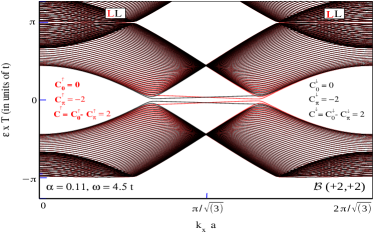
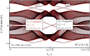
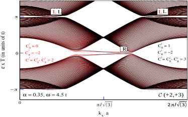
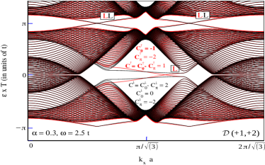
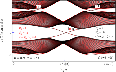
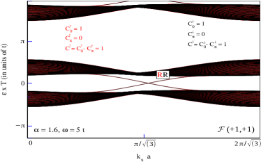
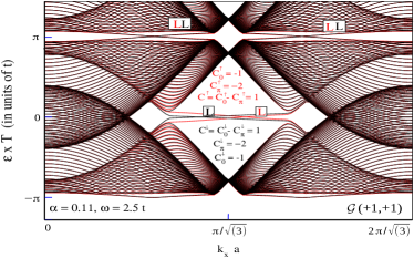
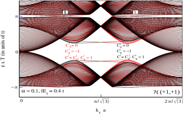
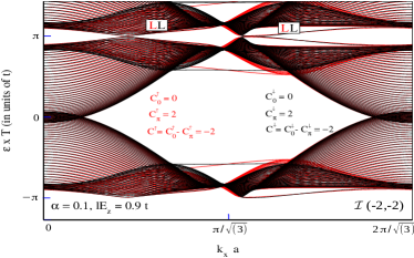
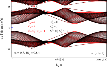
Figure 6:

References

- (1) T. Oka and H. Aoki, Phys. Rev. B 79, 081406(R) (2009).
- (2) T. Kitagawa, E. Berg, M. Rudner, and E. Demler, Phys. Rev. B 82, 235114 (2010).
- (3) Z. Gu, H.A. Fertig, D. P. Arovas, and A. Auerbach, Phys. Rev. Lett. 107, 216601 (2011).
- (4) N. H. Lindner, G. Refael, and V. Galitski, Nature Phys. 7, 490 (2011).
- (5) L. Jiang, T. Kitagawa, J. Alicea, A. R. Akhmerov, D. Pekker, G. Refael, J. I. Cirac, E. Demler, M. D. Lukin, and P. Zoller, Phys. Rev. Lett. 106, 220402 (2011).
- (6) H. L. Calvo, H. M. Pastawski, S. Roche and L. E. F. Foa Torres, App. Phys. Lett. 98, 232103 (2011); H. L. Calvo, P. M. Perez-Piskunow, S. Rocje and L. E. F. Foa Torres, App. Phys. Lett. 98, 232103 (2012); H. L. Calvo, P. M. Perez-Piskunow, H. M. Pastawski, S. Roche and L. E. F. Foa Torrres, Jnl of Phys; Cond,. Matt. 25, 144202 (2013).
- (7) B. Dora, J. Cayssol, F. Simon, and R. Moessner, Phys. Rev. Lett. 108, 056602 (2012).
- (8) A. Kundu and B. Seradjeh, Phys. Rev. Lett. 111, 136402 (2013).
- (9) A. Kundu, H.A. Fertig, and B. Seradjeh, Phys. Rev. Lett. 113, 236803 (2014).
- (10) M. Ezawa, Phys. Rev. Lett. 110, 026603 (2013).
- (11) M. S. Rudner, N. H. Lindner, E. Berg and M. Levin, Phys. RevX3, 031005 (2013).
- (12) P. Delplace, A. Gomez-Leon and G. Platero, Phys. Rev. B88, 245422 (2013).
- (13) F. Gallego-Marcos, G. Platero, C. Nietner, G. Schaller, and T. Brandes, Phys. Rev. A90, 033614 (2014).
- (14) D. Carpentier, P. Delplace, M. Fruchart and K. Gawedzki, Phys. Rev. Lett. 114, 106806 (2015).
- (15) M. A. Sentef, M. Claasen, A. F. Kemper, B. Moritz, T. Oka, J. K. Freericks and T. P. Devereaux, Nat. Comm. 6, 7047 (2015).
- (16) M. V. Fistul and K. B. Efetov, Phys. Rev. B90, 125416 (2014).
- (17) L. J. Maczewsky, J. M. Zeuner, S. Nolte and A. Szameit, Nat. Comm. 8, 13756 (2017).
- (18) S. Mukherjee, A. Spracklen, M. Valiente, E. Andersson, P. Ohberg, N. Goldman and R. R. Thomson, Nat. Comm. 8, 13918 (2017).
- (19) M. Ezawa, Phys. Rev. Lett. 110, 026603 (2013).
- (20) S. Konschuh, M. Gmitra, and J. Fabian, Phys. Rev. B 82, 245412 (2010).
- (21) C. L. Kane and E. J. Mele, Phys. Rev. Lett. 95, 146802 (2005).
- (22) M. Z. Hasan and C. L. Kane, Rev. Mod. Phys. 82, 3045 (2010)
- (23) X.-L. Qi and S.C. Zhang, Rev. Mod. Phys. 83, 1057 (2011)
- (24) L. Tao, E. Cinquanta, D. Chiappe, C Grazianetti, M. Fanciulli, M. Dubey, A. Molle and D. Ankinwande, Nat. Nanotechnol. 10, 227 (2015).
- (25) J. Linder and T. Yokoyama, Phys. Rev. B89, 020504(R) (2014).
- (26) S. Rachel and M. Ezawa, Phys. Rev. B89,195303 (2014).
- (27) R. Saxena, A. Saha and S. Rao, Phys. Rev. B92, 245412 (2015).
- (28) G.C.Paul, S. Sarkar and A. Saha,Phys. Rev. B94, 155453 (2016).
- (29) K. Li and Y. Y. Zhang, Phys. Rev. B94, 165441 (2016).
- (30) S. Sarkar, A. Saha and S. Gangadharaiah, archive preprint, 1609.00693.
- (31) P. Mohan, R. Saxena, A. Kundu and S. Rao, Phys. Rev. B94, 235419 (2016).
- (32) T. Mikami, S. Kitamura, K. Yasuda, N. Tsuji, T. Oka, and H. Aoki, Phys. Rev. B 93, 144307 (2016).
- (33) Y. Xiang Wang, F. Li, Physica B, Volume 492, 1 July 2016, Pages 1-6
- (34) Z. Yi-Fu, Y. Yun-You, J. Yan, S. Li, S. Rui, S. Dong-Ning and X. Ding-Yu, Chinese Physics B 22, Number 11.
- (35) F. Grusdt, T. Li, I. Bloch, E. Demler, Phys. Rev. A 95, 063617 (2017)
- (36) L. Dong, L. Zhou, B. Wu, B. Ramachandran, H. Pu, Phys. Rev. A 89, 011602 (2014)
- (37) Y. J. Lin, K. Jimenez-Garcia, I. B. Spielman, Nature (London) 471, 83 (2011)
- (38) Y.-J. Lin, R. L. Compton, K. Jimenez-Garcia, W. D. Phillips, J. V. Porto, I. B. Spielman, Nature Phys. 7, 531 (2011)
- (39) P. Wang, Z.-Q. Yu, Z. Fu, J. Miao, L. Huang, S. Chai, H. Zhai, J. Zhang, Phys. Rev. Lett. 109, 095301 (2012)
- (40) L. W. Cheuk, A. T. Sommer, Z. Hadzibabic, T. Yefsah, W. S. Bakr, M. W. Zwierlein, Phys. Rev. Lett. 109, 095302 (2012)
- (41) P. M. Perez-Piskunow, L. E. F. Foa Torres, and G. Usaj, Physical Review A bf 91, 043625 (2015).
- (42) P. M. Perez-Piskunow, G. Usaj, C. A. Balseiro, and L. E. F. Foa Torres Physical Review B, 89, 121401(R) (2014).
- (43) L. E. F. Foa Torres, P. M. Perez-Piskunow, C. A. Balseiro, G. Usaj Phys. Rev. Lett. 113, 266801 (2014).
- (44) J. Atteia, J. H. Bardarson and J. Cayssol, arXiv number, 1709.00090.
- (45) B. Mukherjee, P. Mohan, D. Sen and K. Sengupta, arxiv number, 1709.06554.
- (46) M. Rodriguez-Vega and B. Seradjeh, arxiv number, 1706.05303.
- (47) T. Fukui, Y. Hatsugai, and H. Suzuki, J. Phys. Soc. Jpn. 74, (2005) pp. 1674-1677.
- (48) P. Titum, E. Berg, M. S. Rudner, G. Refael, and N. H. Lindner, Phys. Rev. X 6, 021013 (2016).
- (49) A. Quelle, C. Weitenberg, K. Sengstock, and C. Morais Smith, arXiv:1704.00306.
- (50) A. Kundu, M. Rudner, E. Berg, N. H. Lindner, arXiv:1708.05023.
- (51) Aaron Farrell and T. Pereg-Barnea Phys. Rev. Lett. 115, 106403 (2015).
- (52) Aaron Farrell and T. Pereg-Barnea Phys. Rev. B 93, 045121 (2016).
- (53) H. H. Yap, L. Zhou, J.-S. Wang, and J. Gong, Phys. Rev. B 96, 165443 (2017).
- (54) M. A. Sentef, M. Claassen, A. F. Kemper, B. Moritz, T. Oka, J. K. Freericks T. P. Devereaux, Nature Communications 6, Article number: 7047 (2015)
- (55) C. L. Kane, E. J. Mele, PRL 95, 226801 (2005)
- (56) Ruchi Saxena, Arijit Saha, Sumathi Rao PRB 92, 245412 (2015)
- (57) A. Hattori, S. Tanaya, K. Yada, M. Araidai, M. Sato, Y. Hatsugai, K. Shiraishi and Y. Tanaka, J. Phys.:Condens. Matter 29, 115302 (2017)
- (58) M. C. Rechtsman, J. M. Zeuner, Y. Plotnik, Y. Lumer, D. Podolsky, F. Dreisow, S. Nolte, M. Segev A. Szameit, Nature 496, 196-200 (2013)
- (59) P. Titum, N. H. Lindner, M. C. Rechtsman, G. Refael PRL 114 (5), 056801 (2015)
- (60) A. Quelle, C. Weitenberg , K. Sengstock and C. M. Smith, New J. Phys. 19 113010 (2017)