Approximability of the Six-vertex Model

Abstract

In this paper we take the first step toward a classification of the approximation complexity of the six-vertex model, an object of extensive research in statistical physics. Our complexity results conform to the phase transition phenomenon from physics. We show that the approximation complexity of the six-vertex model behaves dramatically differently on the two sides separated by the phase transition threshold. Furthermore, we present structural properties of the six-vertex model on planar graphs for parameter settings that have known relations to the Tutte polynomial $T(G;x,y)$.

1 Introduction

Six-vertex models originate in statistical mechanics as a family of vertex models for crystal lattices with hydrogen bonds. Classically it is defined on a planar lattice region where each vertex of the lattice is connected by an edge to four “nearest neighbors”. A state of the model consists of an arrow on each edge such that the number of arrows pointing inwards at each vertex is exactly two. This 2-in-2-out law on the arrow configurations is called the ice rule [Sla41]. Thus there are six permitted types of local configurations around a vertex—hence the name six-vertex model (see Figure 1). In graph theoretic terms, the states are Eulerian orientations of the underlying undirected graph.

(a) $1$

(b) $2$

(c) $3$

(d) $4$

(e) $5$

(f) $6$

Figure 1: Valid configurations of the six-vertex model.

In general, the six configurations 1 to 6 in Figure 1 are associated with six possible weights $w_{1},\ldots,w_{6}$. We will follow convention in physics and assume arrow reversal symmetry, i.e. $w_{1}=w_{2}=a,w_{3}=w_{4}=b$ and $w_{5}=w_{6}=c$. In this paper we assume $a,b,c\geq 0$, as is assumed in classical physics. The partition function of the six-vertex model with parameters $(a,b,c)$ on a 4-regular graph $G$, where incident edges of each vertex are labeled 1 to 4, is defined as

$$Z(G;a,b,c)=\sum_{\tau\in\mathcal{EO}(G)}a^{n_{1}+n_{2}}b^{n_{3}+n_{4}}c^{n_{5}+n_{6}},$$

where $\mathcal{EO}(G)$ is the set of all Eulerian orientations of $G$, and $n_{i}$ is the number of vertices in type $i$ ($1\leq i\leq 6$) in the graph under an Eulerian orientation $\tau\in\mathcal{EO}(G)$.

The first such models were introduced by Linus Pauling [Pau35] in 1935 to describe the properties of ice. In 1967, Elliot Lieb [Lie67c, Lie67a, Lie67b] famously showed that, for parameters $(a,b,c)=(1,1,1)$ on the square lattice graph, as the side $N$ of the square approaches $\infty$, the value of the “partition function per vertex” $W=Z^{1/N^{2}}$ approaches $\left(\frac{4}{3}\right)^{3/2}\approx 1.5396007\ldots$ (Lieb’s square ice constant). This is called an exact solution of the model, and is considered a triumph. After that, exact solutions for other lattice type graphs (such as [Sut67, FW70]) have been obtained in the limiting sense.

For half a century, the six-vertex model has fascinated physicists, chemists, mathematicians and others . Beyond physics, connections of the six-vertex model to many other areas are discovered. For example, Zeilberger [Zei96] proved the famous alternating sign matrix (ASM) conjecture in combinatorics, and Kuperberg [Kup96] gave a simplified proof making a connection to the six-vertex model.

The six-vertex model is also known to be related to the Tutte polynomial [EMM11] in at least two points. It is known [Tut54] that $T(G;0,-2)$ is the number of Eulerian orientations, i.e., $T(G;0,-2)=Z(G;1,1,1)=|\mathcal{EO}(G)|$, for every 4-regular graph $G$. Another link was proved by Las Vergnas [Ver88] that $Z(H;1,1,2)=2T(G;3,3)$ for any plane graph $G$ with medial graph $H$.

Recently, the exact computational complexity of six-vertex models has been investigated. This is studied in the context of a classification program for the complexity of counting problems, where the six-vertex models serve as important basic (asymmetric) cases for Holant problems [CFS17]. It is shown that there are some surprising P-time computable settings, but for most parameters computing the partition function $Z(G;a,b,c)$ exactly is #P-hard. Under our parameterization of $a,b,c$ being nonnegative (as is the case in the classical setting), the only P-time computable cases are: (1) two of $a,b,c$ are zero or (2) one of $a,b,c$ is zero and the other two are equal. Evaluation at any other point for a general graph is #P-hard. On planar graphs it is also P-time computable for parameter settings $(a,b,c)$ that satisfy $c^{2}=a^{2}+b^{2}$. All other non-trivial P-time computable cases require cancellations (for real or complex parameters $(a,b,c)$) and do not apply for nonnegative $a,b,c$. Mihail and Winkler first proved that computing the number of unweighted Eulerian orientations is #P-complete over general graphs [MW96]. Huang and Lu proved that it remains #P-complete for even degree regular (but not necessarily planar) graphs [HL16]. Guo and Williams improved it to planar $4$-regular graphs [GW13]. The latter is equivalent to computing the partition function of the six-vertex model on planar graphs with the parameter setting $(1,1,1)$.

In terms of approximate complexity, results are limited. To our best knowledge, there are only a very few papers that relate to the approximate complexity of the six-vertex model, and they are all on unweighted Eulerian orientations. Mihail and Winkler’s pioneering work [MW96] gave the first fully polynomial randomized approximation scheme (FPRAS) for the number of Eulerian orientations on a general graph. Luby, Randall, and Sinclair presented an elegant proof of the rapid mixing of a Markov chain that leads to a fully polynomial almost uniform sampler (FPAUS) for Eulerian orientations on any region of the Cartesian lattice with fixed boundaries [LRS01]. Randall and Tetali [RT00] used a comparison technique to prove the single-site Glauber dynamics is rapidly mixing on the same lattice graph, by relating this Markov chain to the Luby-Randall-Sinclair chain. Goldberg, Martin, and Paterson [GMP04] further extended the technique by Randall and Tetali to prove that the single-site Glauber dynamics is rapidly mixing for the free-boundary case on lattice graphs.

The known results on approximate complexity for the six-vertex model are all for the unweighted case, which is the point $(1,1,1)$ in the six-vertex model. In this paper we initiate a study toward a classification of the approximate complexity of the six-vertex model in terms of the parameters. Our results conform to phase transitions in physics.

Here we briefly describe the phenomenon of phase transition of the zero-field six-vertex model (see Baxter’s book [Bax82] for more details). On square-lattice in the thermodynamic limit: (1) When $a>b+c$ (FE: ferroelectric phase) any finite region tends to be frozen into one of the two configurations where either all arrows point up or to the right (Figure 1-1), or all point down or to the left (Figure 1-2). (2) Symmetrically when $b>a+c$ (also FE) all arrows point down or to the right (Figure 1-3), or all point up or to the left (Figure 1-4). (3) When $c>a+b$ (AFE: anti-ferroelectric phase) configurations in Figure 1-5 and Figure 1-6 alternate. (4) When $c<a+b$, $b<a+c$, and $a<b+c$, the system is disordered (DO: disordered phase) in the sense that all correlations decay to zero with increasing distance; in particular on the dashed curve $c^{2}=a^{2}+b^{2}$ the model can be solved by Pfaffians exactly [FW70], and the correlations decay inverse polynomially, rather than exponentially, in distance. See Figure 2(a).

(a) Phase diagram of the six-vertex model.

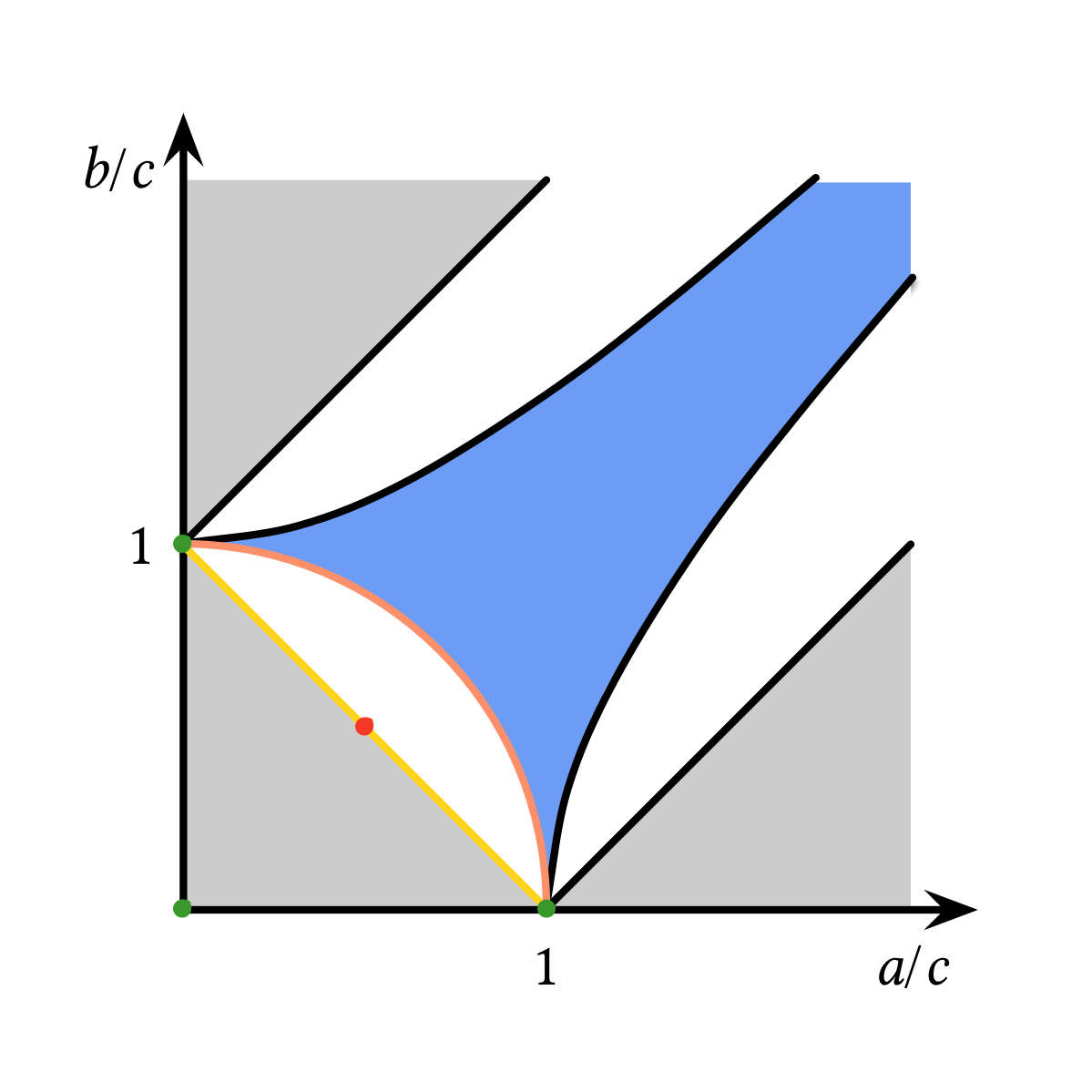
(b) Complexity diagram of the six-vertex model.

Figure 2:

In Figure 2(b) we have a corresponding complexity landscape.

Theorem 1.1.

There is an FPRAS for $Z(G;a,b,c)$ if $a^{2}\leq b^{2}+c^{2}$, $b^{2}\leq a^{2}+c^{2}$, and $c^{2}\leq a^{2}+b^{2}$ (the blue region). There is no FPRAS for $Z(G;a,b,c)$ if $a>b+c$ or $b>a+c$ or $c>a+b$ (the grey region), unless RP $=$ NP.

Our FPRAS result is actually stronger in that the FPRAS works even if different signatures from the blue region are assigned at different vertices. The blue region is a proper subset of the disordered phase. The point $(1,1,1)$ is contained in this region, which is the only previously known approximable case. The hardness part (the grey region) coincides with the FE/AFE phases. The three green points together with a point at infinity ($(a,b,c)=(1,1,0)$) are exactly P-time computable. All parameters belonging to the orange curve $c^{2}=a^{2}+b^{2}$ are exactly P-time computable on planar graphs. Computing for the six-vertex model at $(1/2,1/2,1)$ (the red point) is equivalent to evaluating the Tutte polynomial $T(G;3,3)$ on planar graphs. Note that any 4-regular plane graph $H$ is the medial graph of some plane graph $G$. The approximation complexity for the white region is unknown.

Furthermore, we show that there is a fundamental structural difference in the behavior on the two sides separated by the phase transition threshold, in terms of closure properties. Gadget construction is a common technique used in approximation-preserving reductions [DGGJ04]. If a constraint function $g$ can be expressed by a polynomial-size gadget using a constraint function $f$, then the approximation complexity of $g$ is no harder than that of $f$. In Theorem 3.1 of Section 3, we prove that the set of 4-ary functions lying in the combined region of blue and white (this is the same as the DO region in Figure 2(a)) is closed under gadget construction. In Theorem 3.2 we prove that the set of 4-ary functions lying on the yellow line (phase transition threshold for AFE and DO) is closed under planar gadget construction. Theorem 3.1 is also used in proving a Markov chain is rapidly mixing in Section 4.

Our FPRAS also has implications for counting weighted sum of directed Eulerian partitions (partition of edges of $G$ into directed edge-disjoint circuits). A special case is an FPRAS for this weighted sum when the weight of is at least $\sqrt{2}-1$ (more on the connection between directed Eulerian partitions and the three types of pairings , , and can be found in Section 3).

Our proof uses the Holant framework. In Section 2 we express the six-vertex model as a Holant problem. This allows us to use techniques developed in the study of Holant problems to make progress in both fronts: We design a rapidly mixing Markov chain to derive a FPRAS in the blue region (within the disordered phase). This result can also be obtained by using a technique called windable by McQuillan [McQ13], specifically developed for the Holant framework. We also use techniques developed in the Holant framework to prove NP-hardness of approximation for the six-vertex model in the grey region (coincide with the ferroelectric/anti-ferroelectric phases). These are the first inapproximability results for the six-vertex model.

2 Preliminaries

2.1 Six-Vertex Model as a Holant Problem

The six-vertex model is naturally expressed as a Holant problem, which we define as follows. A function $f:\left\{0,1\right\}^{k}\rightarrow\mathbb{C}$ is called a constraint function, or a signature, of arity $k$. In this paper we restrict $f$ to take nonnegative values in $\mathbb{R}^{+}$. Fix a set $\mathcal{F}$ of constraint functions. A signature grid $\Gamma=(G,\xi)$ is a tuple, where $G=(V,E)$ is a graph, $\xi$ labels each $v\in V$ with a function $f_{v}\in\mathcal{F}$ of arity $\operatorname{deg}(v)$, and the incident edges $E(v)$ at $v$ are identified as input variables to $f_{v}$, also labeled by $\xi$. Every assignment $\sigma:E\rightarrow\left\{0,1\right\}$ gives an evaluation $\prod_{v\in V}f_{v}\left(\sigma|_{E(v)}\right)$, where $\sigma|_{E(v)}$ denotes the restriction of $\sigma$ to $E(v)$. The problem $\operatorname{Holant}\left(\mathcal{F}\right)$ on an instance $\Gamma$ is to compute $\operatorname{Holant}\left(\Gamma;\mathcal{F}\right)=\sum_{\sigma:E\rightarrow\left\{0,1\right\}}\prod_{v\in V}f_{v}\left(\sigma|_{E(v)}\right)$. When $\mathcal{F}=\left\{f\right\}$ is a singleton set, we write $\operatorname{Holant}\left(f\right)$ for simplicity. We use $\operatorname{Holant}\left(\mathcal{F}|\mathcal{G}\right)$ for Holant problems over signature grids with a bipartite graph $(U,V,E)$ where each vertex in $U$ (or $V$) is assigned a signature in $\mathcal{F}$ (or $\mathcal{G}$, respectively).

To write the six-vertex model on a 4-regular graph $G=(V,E)$ as a Holant problem, consider the edge-vertex incidence graph $G^{\prime}=(U_{E},U_{V},E^{\prime})$ of $G$. We model the orientation of an edge in $G$ by putting the Disequality signature $(\neq_{2})$ (which outputs 1 on inputs 01, 10 and outputs 0 on 00, 11) on $U_{E}$ in $G^{\prime}$. We say an orientation on edge $e=\left\{w,v\right\}\in E$ is going out $w$ and into $v$ in $G$ if the edge $(u_{e},u_{w})\in E^{\prime}$ in $G^{\prime}$ takes value $1$ (and $(u_{e},u_{v})\in E^{\prime}$ takes value $0$). An arity-4 signature $f$ on input $x_{1},x_{2},x_{3},x_{4}$ has the signature matrix $M(f)=M_{x_{1}x_{2},x_{4}x_{3}}(f)=\left[\begin{smallmatrix}f_{0000}&f_{0010}&f_{0001}&f_{0011}\\ f_{0100}&f_{0110}&f_{0101}&f_{0111}\\ f_{1000}&f_{1010}&f_{1001}&f_{1011}\\ f_{1100}&f_{1110}&f_{1101}&f_{1111}\end{smallmatrix}\right]$, where the order reversal $x_{4}x_{3}$ is for the convenience of composing these signatures in a planar fashion, by matrix product. At a vertex $v$ in $G$, if we locally index the left, down, right, and up edges incident to $v$ by 1, 2, 3, and 4, respectively, then the constraint by the six-vertex model as specified in Figure 1 can be expressed perfectly as a signature $f$ with $M(f)=\left[\begin{smallmatrix}0&0&0&a\\ 0&b&c&0\\ 0&c&b&0\\ a&0&0&0\end{smallmatrix}\right]$. Thus computing the partition function $Z(G;a,b,c)$ is equivalent to evaluating $\operatorname{Holant}\left(G^{\prime};\neq_{2}|f\right)$ for this $f$.

For convenience in presenting our theorems and proofs, we adopt the following notations assuming $a,b,c\in\mathbb{R}^{+}$. We assume $f$ has signature matrix $M(f)=\left[\begin{smallmatrix}&&&a\\ &b&c&\\ &c&b&\\ a&&&\end{smallmatrix}\right]$.

• $\mathcal{F}_{\leq^{2}}:=\{f\;|\;a^{2}\leq b^{2}+c^{2},~{}~{}b^{2}\leq a^{2}+c^{2},~{}~{}c^{2}\leq a^{2}+b^{2}\}$;

• $\mathcal{F}_{\leq}~{}:=\{f\;|\;a\leq b+c,~{}~{}b\leq a+c,~{}~{}c\leq a+b\}$;

• $\mathcal{F}_{=}~{}:=\{f\;|\;c=a+b\}$;

• $\mathcal{F}_{>}~{}:=\{f\;|\;a>b+c~{}\text{ or }~{}b>a+c~{}\text{ or }~{}c>a+b\text{ where }a,b,c>0\}$.

Remark 2.1.

$\mathcal{F}_{\leq^{2}}\subset\mathcal{F}_{\leq}$.

2.2 Approximation Algorithms

If a counting problem is #P-hard, we may still hope that the problem can be approximated. Suppose $f:\Sigma^{*}\rightarrow\mathbb{R}$ is a function mapping problem instances to real numbers. A fully polynomial randomized approximation scheme (FPRAS) [KL83] for a problem is a randomized algorithm that takes as input an instance $x$ and $\varepsilon>0$, running in time polynomial in $n$ (the input length) and $\varepsilon^{-1}$, and outputs a number $Y$ (a random variable) such that

$$\operatorname{Pr}\left[(1-\varepsilon)f(x)\leq Y\leq(1+\varepsilon)f(x)\right]\geq\frac{3}{4}.$$

3 Confinement Theorems

Theorem 3.1.

If $f$ is the signature of a $4$-ary gadget on the right hand side of $\operatorname{Holant}\left(\neq_{2}|\mathcal{F}_{\leq}\right)$, then $f\in\mathcal{F}_{\leq}$.

Theorem 3.2.

If $f$ is the signature of a $4$-ary plane gadget on the right hand side of $\operatorname{Holant}\left(\neq_{2}|\mathcal{F}_{=}\right)$, then $f\in\mathcal{F}_{=}$.

Before proving Theorem 3.1 and Theorem 3.2, we introduce another view of the six-vertex model. A valid configuration in the six-vertex model, i.e. a weighted Eulerian orientation, can also be viewed as a combination of weighted directed Eulerian partitions. An Eulerian partition of a graph $G$ is a partition of the edges of $G$ into edge-disjoint circuits (in which vertices may repeat whereas edges cannot). A directed Eulerian partition is an Eulerian partition where every edge-disjoint circuit takes one of the two cyclic orientations. Let $G=(V,E)$ be a 4-regular graph and $v$ be a vertex of $G$. Let $e_{1},e_{2},e_{3},e_{4}$ be the four edges incident to $v$. A pairing $\varrho$ at $v$ is a partition of $\{e_{1},e_{2},e_{3},e_{4}\}$ into pairs. There are exactly three distinct pairings at $v$ (Figure 3) which we denote by three special symbols: $\raisebox{-1.20007pt}{\includegraphics[height=8.39996pt,width=8.39996pt,keepaspectratio]{sub_1}},\raisebox{-1.20007pt}{\includegraphics[height=8.39996pt,width=8.39996pt,keepaspectratio]{sub_2}},\raisebox{-1.20007pt}{\includegraphics[height=8.39996pt,width=8.39996pt,keepaspectratio]{sub_3}}$, respectively. An Eulerian partition of $G$ can be uniquely determined by a family of pairings $\varphi=\{\varrho_{v}\}_{v\in V}$, where $\varrho_{v}\in\{\raisebox{-1.20007pt}{\includegraphics[height=8.39996pt,width=8.39996pt,keepaspectratio]{sub_1}},\raisebox{-1.20007pt}{\includegraphics[height=8.39996pt,width=8.39996pt,keepaspectratio]{sub_2}},\raisebox{-1.20007pt}{\includegraphics[height=8.39996pt,width=8.39996pt,keepaspectratio]{sub_3}}\}$ is a pairing at $v$—once the pairing at each vertex is fixed, then the two edges paired together at each vertex is also adjacent in the same circuit.

(a)

(b)

(c)

Figure 3: Pairings at a degree 4 vertex.

For any vertex $v$ in a valid configuration $\tau$ of the six-vertex model (where ice rule is satisfied), incoming edges can be paired with outgoing edges in exactly two ways, corresponding to two of the three pairings at $v$. For example, the configuration in Figure 1-1 of the six-vertex model has two underlying pairings, and . Therefore, $\tau$ can be decomposed into $2^{|V|}$ distinct directed Eulerian partitions denoted by $\Phi(\tau)$. Since no two Eulerian orientations share one directed Eulerian partition and every directed Eulerian partition corresponds to a particular Eulerian orientation, the map from six-vertex configurations to directed Eulerian partitions is $1$-to-$2^{|V|}$, non-overlapping, and surjective. Define $w$ to be a function assigning a weight to every pairing at every vertex and let the weight $\tilde{w}(\varphi)$ of an Eulerian partition $\varphi$, undirected or directed, be the product of weights at each vertex. In particular, when $w$ is defined such that $\left\{\begin{smallmatrix}w(\raisebox{-1.20007pt}{\includegraphics[height=12.0pt,width=12.0pt,keepaspectratio]{sub_1}})=\frac{-a+b+c}{2}\\ w(\raisebox{-1.20007pt}{\includegraphics[height=12.0pt,width=12.0pt,keepaspectratio]{sub_2}})=\frac{a-b+c}{2}\\ w(\raisebox{-1.20007pt}{\includegraphics[height=12.0pt,width=12.0pt,keepaspectratio]{sub_3}})=\frac{a+b-c}{2}\end{smallmatrix}\right.$, or equivalently $\left\{\begin{smallmatrix}a=w(\raisebox{-1.20007pt}{\includegraphics[height=12.0pt,width=12.0pt,keepaspectratio]{sub_2}})+w(\raisebox{-1.20007pt}{\includegraphics[height=12.0pt,width=12.0pt,keepaspectratio]{sub_3}})\\ b=w(\raisebox{-1.20007pt}{\includegraphics[height=12.0pt,width=12.0pt,keepaspectratio]{sub_1}})+w(\raisebox{-1.20007pt}{\includegraphics[height=12.0pt,width=12.0pt,keepaspectratio]{sub_3}})\\ c=w(\raisebox{-1.20007pt}{\includegraphics[height=12.0pt,width=12.0pt,keepaspectratio]{sub_1}})+w(\raisebox{-1.20007pt}{\includegraphics[height=12.0pt,width=12.0pt,keepaspectratio]{sub_2}})\end{smallmatrix}\right.$, for every vertex with signature matrix $\left[\begin{smallmatrix}&&&a\\ &b&c&\\ &c&b&\\ a&&&\end{smallmatrix}\right]$, then the weight of a six-vertex model configuration $\tau$ is equal to $\sum_{\varphi\in\Phi(\tau)}\tilde{w}(\varphi)$, by expressing a product of sums as a sum of products.

The connection between Eulerian orientations and Eulerian partitions on 4-regular graphs has been explored. Las Vergnas [Ver88] demonstrated a special case for plane graphs: the number of directed non-intersecting Eulerian partitions is equal to the number of Eulerian orientations with weight 2 on every saddle configuration (Figure 1-5 1-6), which is the six-vertex model at (1, 1, 2) . Jaeger [Jae90] proposed a graph polynomial called transition polynomial as a generalization of weighted Eulerian partitions, and related it with weighted Eulerian orientations. The idea of unweighted directed Eulerian partitions was implicitly used in Mihail and Winkler’s paper [MW96] to approximate the number of unweighted Eulerian orientations, where they also adopted the notion of pairings.

Proof of Theorem 3.1.

For the signature $f$ of a 4-ary gadget on the right hand side of $\operatorname{Holant}\left(\neq_{2}|\mathcal{F}_{\leq}\right)$ (Figure 4(a)), we first show that its signature matrix must be of the form $\left[\begin{smallmatrix}&&&a^{\prime}\\ &b^{\prime}&c^{\prime}&\\ &c^{\prime}&b^{\prime}&\\ a^{\prime}&&&\end{smallmatrix}\right]$. First, $f$ still obeys the ice rule, i.e. it cannot take nonzero values on inputs with Hamming weight not 2. Including the dangling edges, every vertex has exactly two incoming edges and two outgoing edges. Thus if we sum the in-degrees over all vertices, it must equal to the sum of out-degrees over all vertices, i.e., $\sum_{v}{\rm in\text{-}deg}(v)=\sum_{v}{\rm out\text{-}deg}(v)$. Every internal edge contributes exactly 1 to each sum. Thus the number of incoming dangling edges is equal to the number of outgoing dangling edges, which must be 2 each since they sum to 4. Second, $f$ still satisfies arrow reversal symmetry. For any valid orientation of edges in the gadget contributing a nonnegative factor to $f(x)$, reversing the orientations on all edges will contribute the same factor to $f(\overline{x})$, as is true for every signature on a single vertex of degree 4.

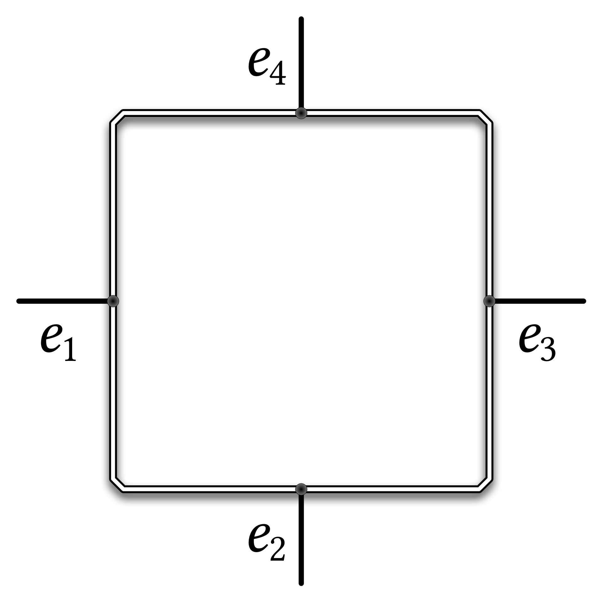
(a)

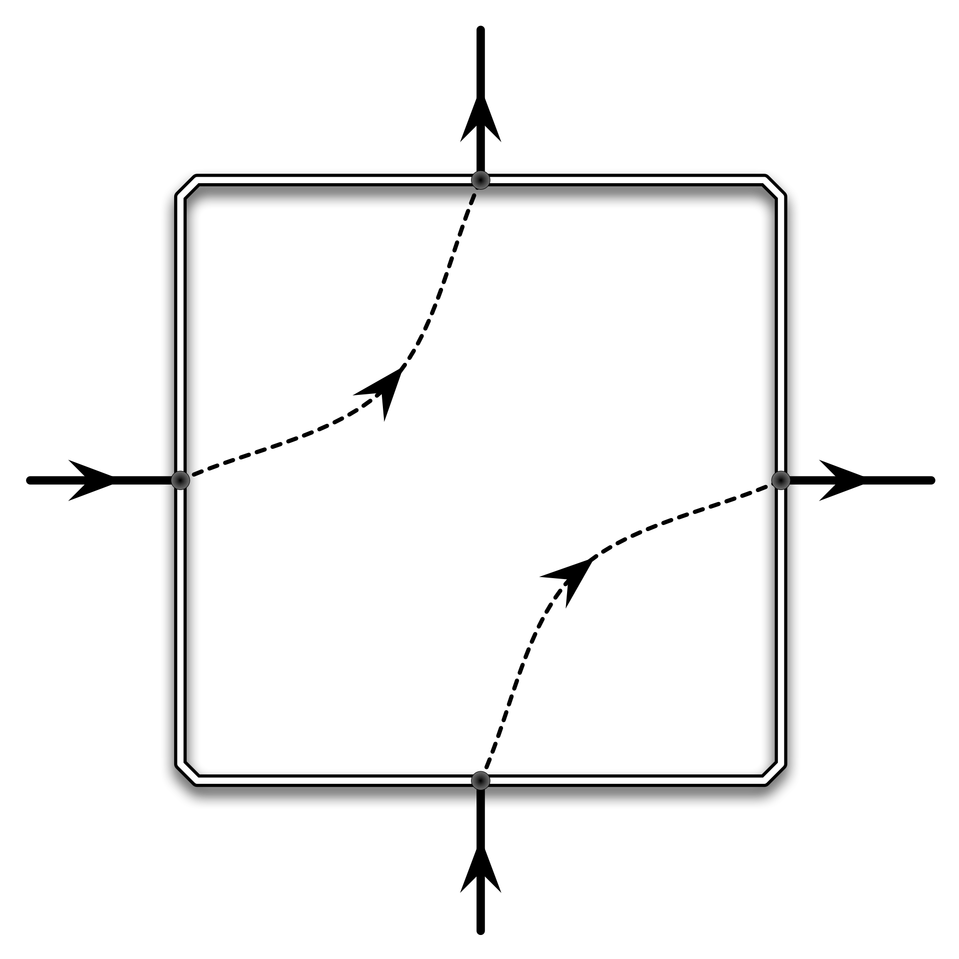
(b)

(c)

Figure 4: A gadget constructed on the right hand side of $\operatorname{Holant}\left(\neq_{2}|\mathcal{F}_{\leq}\right)$.

The notion of Eulerian partitions previously used for graphs can also be defined for gadgets. An Eulerian partition for a gadget $g$ with four dangling edges is a partition of the edges in $g$ into edge-disjoint circuits and exactly two walks (in which vertices may repeat whereas edges cannot) whose ends are exactly the four dangling edges. The weight $\tilde{w}$ of such an Eulerian partition $\varphi$ can be similarly defined. Set $w$ such that $\left\{\begin{smallmatrix}w(\raisebox{-1.20007pt}{\includegraphics[height=12.0pt,width=12.0pt,keepaspectratio]{sub_1}})=\frac{-a+b+c}{2}\\ w(\raisebox{-1.20007pt}{\includegraphics[height=12.0pt,width=12.0pt,keepaspectratio]{sub_2}})=\frac{a-b+c}{2}\\ w(\raisebox{-1.20007pt}{\includegraphics[height=12.0pt,width=12.0pt,keepaspectratio]{sub_3}})=\frac{a+b-c}{2}\end{smallmatrix}\right.$, or equivalently $\left\{\begin{smallmatrix}a=w(\raisebox{-1.20007pt}{\includegraphics[height=12.0pt,width=12.0pt,keepaspectratio]{sub_2}})+w(\raisebox{-1.20007pt}{\includegraphics[height=12.0pt,width=12.0pt,keepaspectratio]{sub_3}})\\ b=w(\raisebox{-1.20007pt}{\includegraphics[height=12.0pt,width=12.0pt,keepaspectratio]{sub_1}})+w(\raisebox{-1.20007pt}{\includegraphics[height=12.0pt,width=12.0pt,keepaspectratio]{sub_3}})\\ c=w(\raisebox{-1.20007pt}{\includegraphics[height=12.0pt,width=12.0pt,keepaspectratio]{sub_1}})+w(\raisebox{-1.20007pt}{\includegraphics[height=12.0pt,width=12.0pt,keepaspectratio]{sub_2}})\end{smallmatrix}\right.$. Observe that if a vertex has a signature $f\in\mathcal{F}_{\leq}$, then the weight of every pairing is nonnegative, and the weight of any directed Eulerian partition of a graph/gadget comprised of such vertices is also nonnegative.

Under the six-vertex model, for any specific configuration $\tau$ of the gadget with signature $f$ that contributes a nonzero factor to $f(0011)$ when $e_{1},e_{2}$ go in and $e_{3},e_{4}$ go out, it can be viewed as a weighted sum of directed Eulerian partitions $\Phi(\tau)$. For every Eulerian partition $\varphi\in\Phi(\tau)$, the two directed walks are either $\{e_{1}\leadsto e_{4},e_{2}\leadsto e_{3}\}$ (Figure 4(b)) or $\{e_{1}\leadsto e_{3},e_{2}\leadsto e_{4}\}$. Denote by $\Phi_{0011,\raisebox{-1.20007pt}{\includegraphics[height=8.39996pt,width=8.39996pt,keepaspectratio]{sub_2}}}$ the set of directed Eulerian partitions (distributed in potentially many different six-vertex configurations), each of which has directed walks $\{e_{1}\leadsto e_{4},e_{2}\leadsto e_{3}\}$; denote by $\Phi_{0011,\raisebox{-1.20007pt}{\includegraphics[height=8.39996pt,width=8.39996pt,keepaspectratio]{sub_3}}}$ the set of directed Eulerian partitions, each of which has directed walks $\{e_{1}\leadsto e_{3},e_{2}\leadsto e_{4}\}$. In terms of directed Eulerian partitions of the gadget, $f(0011)$ can be seen as the weighted sum of elements from two disjoint sets $\Phi_{0011,\raisebox{-1.20007pt}{\includegraphics[height=8.39996pt,width=8.39996pt,keepaspectratio]{sub_2}}}$ and $\Phi_{0011,\raisebox{-1.20007pt}{\includegraphics[height=8.39996pt,width=8.39996pt,keepaspectratio]{sub_3}}}$. Defining the weight of a set $\Phi$ of directed Eulerian partitions by $W(\Phi)=\sum_{\varphi\in\Phi}\tilde{w}(\varphi)$ yields $f(0011)=W(\Phi_{0011,\raisebox{-1.20007pt}{\includegraphics[height=8.39996pt,width=8.39996pt,keepaspectratio]{sub_2}}})+W(\Phi_{0011,\raisebox{-1.20007pt}{\includegraphics[height=8.39996pt,width=8.39996pt,keepaspectratio]{sub_3}}})$, and similarly $f(1100)=W(\Phi_{1100,\raisebox{-1.20007pt}{\includegraphics[height=8.39996pt,width=8.39996pt,keepaspectratio]{sub_2}}})+W(\Phi_{1100,\raisebox{-1.20007pt}{\includegraphics[height=8.39996pt,width=8.39996pt,keepaspectratio]{sub_3}}})$. Note that there is a bijective weight-preserving map between $\Phi_{0011,\raisebox{-1.20007pt}{\includegraphics[height=8.39996pt,width=8.39996pt,keepaspectratio]{sub_2}}}$ and $\Phi_{1100,\raisebox{-1.20007pt}{\includegraphics[height=8.39996pt,width=8.39996pt,keepaspectratio]{sub_2}}}$ by reversing the direction of every circuit and walk of an Eulerian partition. That is to say, $W(\Phi_{0011,\raisebox{-1.20007pt}{\includegraphics[height=8.39996pt,width=8.39996pt,keepaspectratio]{sub_2}}})=W(\Phi_{1100,\raisebox{-1.20007pt}{\includegraphics[height=8.39996pt,width=8.39996pt,keepaspectratio]{sub_2}}})$ and similarly $W(\Phi_{0011,\raisebox{-1.20007pt}{\includegraphics[height=8.39996pt,width=8.39996pt,keepaspectratio]{sub_3}}})=W(\Phi_{1100,\raisebox{-1.20007pt}{\includegraphics[height=8.39996pt,width=8.39996pt,keepaspectratio]{sub_3}}})$. This proves that $f(0011)=f(1100)$, as we noted earlier. Similar conclusions can be made for the other two pairs of values $\{f(0110),f(1001)\}$ and $\{f(0101),f(1010)\}$.

An important observation is that for each Eulerian partition in $\Phi_{0011,\raisebox{-1.20007pt}{\includegraphics[height=8.39996pt,width=8.39996pt,keepaspectratio]{sub_2}}}$, if we only reverse the walk from $e_{1}\leadsto e_{4}$ to $e_{4}\leadsto e_{1}$ and keep the directions on all circuits and the other walk unchanged, this Eulerian partition has the same weight but now lies in $\Phi_{1010,\raisebox{-1.20007pt}{\includegraphics[height=8.39996pt,width=8.39996pt,keepaspectratio]{sub_2}}}$ (Figure 4(c)). This is because at every vertex $v$, reversing any orientation of a branch of the given pairing $\varrho_{v}\in\{\raisebox{-1.20007pt}{\includegraphics[height=8.39996pt,width=8.39996pt,keepaspectratio]{sub_1}},\raisebox{-1.20007pt}{\includegraphics[height=8.39996pt,width=8.39996pt,keepaspectratio]{sub_2}},\raisebox{-1.20007pt}{\includegraphics[height=8.39996pt,width=8.39996pt,keepaspectratio]{sub_3}}\}$ does not change the value $w(\varrho_{v})$. In this way, we set up a one-to-one weight-preserving map between $\Phi_{0011,\raisebox{-1.20007pt}{\includegraphics[height=8.39996pt,width=8.39996pt,keepaspectratio]{sub_2}}}$ and $\Phi_{1010,\raisebox{-1.20007pt}{\includegraphics[height=8.39996pt,width=8.39996pt,keepaspectratio]{sub_2}}}$, i.e. $W(\Phi_{0011,\raisebox{-1.20007pt}{\includegraphics[height=8.39996pt,width=8.39996pt,keepaspectratio]{sub_2}}})=W(\Phi_{1010,\raisebox{-1.20007pt}{\includegraphics[height=8.39996pt,width=8.39996pt,keepaspectratio]{sub_2}}})$. Combining the result in the last paragraph, we can write

• $W(\raisebox{-1.20007pt}{\includegraphics[height=8.39996pt,width=8.39996pt,keepaspectratio]{sub_2}})=W(\Phi_{0011,\raisebox{-1.20007pt}{\includegraphics[height=8.39996pt,width=8.39996pt,keepaspectratio]{sub_2}}})=W(\Phi_{1100,\raisebox{-1.20007pt}{\includegraphics[height=8.39996pt,width=8.39996pt,keepaspectratio]{sub_2}}})=W(\Phi_{0101,\raisebox{-1.20007pt}{\includegraphics[height=8.39996pt,width=8.39996pt,keepaspectratio]{sub_2}}})=W(\Phi_{1010,\raisebox{-1.20007pt}{\includegraphics[height=8.39996pt,width=8.39996pt,keepaspectratio]{sub_2}}})$;

• $W(\raisebox{-1.20007pt}{\includegraphics[height=8.39996pt,width=8.39996pt,keepaspectratio]{sub_1}})=W(\Phi_{0110,\raisebox{-1.20007pt}{\includegraphics[height=8.39996pt,width=8.39996pt,keepaspectratio]{sub_1}}})=W(\Phi_{1001,\raisebox{-1.20007pt}{\includegraphics[height=8.39996pt,width=8.39996pt,keepaspectratio]{sub_1}}})=W(\Phi_{0101,\raisebox{-1.20007pt}{\includegraphics[height=8.39996pt,width=8.39996pt,keepaspectratio]{sub_1}}})=W(\Phi_{1010,\raisebox{-1.20007pt}{\includegraphics[height=8.39996pt,width=8.39996pt,keepaspectratio]{sub_1}}})$;

• $W(\raisebox{-1.20007pt}{\includegraphics[height=8.39996pt,width=8.39996pt,keepaspectratio]{sub_3}})=W(\Phi_{0011,\raisebox{-1.20007pt}{\includegraphics[height=8.39996pt,width=8.39996pt,keepaspectratio]{sub_3}}})=W(\Phi_{1100,\raisebox{-1.20007pt}{\includegraphics[height=8.39996pt,width=8.39996pt,keepaspectratio]{sub_3}}})=W(\Phi_{0110,\raisebox{-1.20007pt}{\includegraphics[height=8.39996pt,width=8.39996pt,keepaspectratio]{sub_3}}})=W(\Phi_{1001,\raisebox{-1.20007pt}{\includegraphics[height=8.39996pt,width=8.39996pt,keepaspectratio]{sub_3}}})$.

Consequently, we have $\left\{\begin{smallmatrix}a^{\prime}=W(\raisebox{-1.20007pt}{\includegraphics[height=12.0pt,width=12.0pt,keepaspectratio]{sub_2}})+W(\raisebox{-1.20007pt}{\includegraphics[height=12.0pt,width=12.0pt,keepaspectratio]{sub_3}})\\ b^{\prime}=W(\raisebox{-1.20007pt}{\includegraphics[height=12.0pt,width=12.0pt,keepaspectratio]{sub_1}})+W(\raisebox{-1.20007pt}{\includegraphics[height=12.0pt,width=12.0pt,keepaspectratio]{sub_3}})\\ c^{\prime}=W(\raisebox{-1.20007pt}{\includegraphics[height=12.0pt,width=12.0pt,keepaspectratio]{sub_1}})+W(\raisebox{-1.20007pt}{\includegraphics[height=12.0pt,width=12.0pt,keepaspectratio]{sub_2}})\end{smallmatrix}\right.$. $W(\raisebox{-1.20007pt}{\includegraphics[height=8.39996pt,width=8.39996pt,keepaspectratio]{sub_2}})$, $W(\raisebox{-1.20007pt}{\includegraphics[height=8.39996pt,width=8.39996pt,keepaspectratio]{sub_1}})$, and $W(\raisebox{-1.20007pt}{\includegraphics[height=8.39996pt,width=8.39996pt,keepaspectratio]{sub_3}})$ are all nonnegative due to the fact that the weight of every directed Eulerian partition has a nonnegative weight. Therefore, $a^{\prime}\leq b^{\prime}+c^{\prime}$, $b^{\prime}\leq a^{\prime}+c^{\prime}$, and $c^{\prime}\leq a^{\prime}+b^{\prime}$. This is to say, $f\in\mathcal{F}_{\leq}$. ∎

Proof of Theorem 3.2.

Inheriting the notations from the above proof, we have $w(\raisebox{-1.20007pt}{\includegraphics[height=8.39996pt,width=8.39996pt,keepaspectratio]{sub_3}})=0$ when $c=a+b$ for each vertex, which is to say no “crossing” can be made at any vertex in any Eulerian partition. Due to planarity, a walk $e_{1}\leadsto e_{3}$ must cross a walk $e_{2}\leadsto e_{4}$ at a vertex, thus $W(\raisebox{-1.20007pt}{\includegraphics[height=8.39996pt,width=8.39996pt,keepaspectratio]{sub_3}})=W(\Phi_{0011,\raisebox{-1.20007pt}{\includegraphics[height=8.39996pt,width=8.39996pt,keepaspectratio]{sub_3}}})=0$. Therefore, $c^{\prime}=a^{\prime}+b^{\prime}$. ∎

Remark 3.1.

Theorem 3.1 not only serves as a depiction of the divergence of six-vertex models under different parameters separated by the phase transition threshold, but also helps us in Section 4 to bound the mixing time of a Markov chain so that approximately counting via sampling [JVV86] leads to an FPRAS.

4 FPRAS

In this section we prove the following theorem.

Theorem 4.1.

There is an FPRAS for computing $\operatorname{Holant}\left(\neq_{2}|\mathcal{F}_{\leq^{2}}\right)$.

For simplicity we prove Theorem 4.1 only for the case where all signatures of arity 4 used in the right-hand side are from a fixed finite subset $\mathcal{F}\subset\mathcal{F}_{\leq^{2}}$, i.e., we show that there is an FPRAS for computing $\operatorname{Holant}\left(\neq_{2}|\mathcal{F}\right)$. With some care the more general statement in Theorem 4.1 can also be proved.

We use the common approach to approximate counting via almost uniform sampling [JVV86] using a rapidly mixing Markov chain [JS89, DFK91, Sin92, Jer03].

Our Markov chain $\mathcal{MC}$ is described in the setting of $\operatorname{Holant}\left(\neq_{2}|\mathcal{F}_{\leq^{2}}\right)$. Let $G=(V,U,E)$ be the underlying bipartite graph of an instance of $\operatorname{Holant}\left(\neq_{2}|\mathcal{F}_{\leq^{2}}\right)$. For simplicity we prove Theorem 4.1 Each vertex in $V$ is assigned $(\neq_{2})$; each vertex $u\in U$ is assigned a signature $f_{u}\in\mathcal{F}_{\leq^{2}}$. An assignment $\sigma$ assigns a value in $\{0,1\}$ to each edge $e\in E$. The state space of $\mathcal{MC}$ is $\Omega=\Omega_{0}\cup\Omega_{2}$, which consists of “perfect” or “near-perfect” assignments to $E$: All assignments satisfy the “two-0 two-1” ice rule at every vertex $u\in U$ of degree 4. We also insist that all assignments satisfy the “one-0 one-1” at every $v\in V$ with possibly exactly two exceptions. Assignments in $\Omega_{0}$ have no exceptions, and are “perfect”. Assignments in $\Omega_{2}$ have exactly two exceptions, and are “near-perfect”. Thus any $\sigma\in\Omega_{0}$ sastifies all $(\neq_{2})$ on $V$, and any $\sigma\in\Omega_{2}$ sastifies all $(\neq_{2})$ on $V-\{v^{\prime},v^{\prime\prime}\}$ for some two vertices $v^{\prime},v^{\prime\prime}\in V$ where it satisfies $(=_{2})$ (which outputs 1 on inputs 00, 11 and outputs 0 on 01, 10).

For any assignment $\sigma\in\Omega$ and any subset $S\subseteq\Omega$, define the weight function $\mathcal{W}$ by $\mathcal{W}(\sigma)=\prod_{u\in U}f_{u}(\sigma|_{E(v)})$ and $\mathcal{Z}(S)=\sum_{\sigma\in S}\mathcal{W}(\sigma)$. Then the Gibbs measure for $\Omega$ is defined by $\pi(\sigma)=\frac{\mathcal{W}(\sigma)}{\mathcal{Z}(\Omega)}$, assuming $\mathcal{Z}(\Omega)>0$. Observe that if a state $\sigma\in\Omega_{2}$ assigns 00 to both edges incident to $v^{\prime}\in V$ (satisfying $(=_{2})$ at $v^{\prime}$) then it must assign 11 to both edges incident to $v^{\prime\prime}\in V$, and vice versa. Indeed, having 00 at $v^{\prime}$ models the fact that $v^{\prime}$ has two arrows going out (to degree-4 vertices in $U$). To maintain the property that the number of incoming arrows is equal to the number of outgoing arrows everywhere else, $v^{\prime\prime}$ must have two arrows coming in, which is equivalent to having 11 at $v^{\prime\prime}$ in the Holant setting. An example state is shown in Figure 6(a).

Transitions in $\mathcal{MC}$ are comprised of three types of moves. Suppose $\sigma\in\Omega_{0}$. An $\Omega_{0}$-to-$\Omega_{2}$ move from $\sigma$ takes a degree 4 vertex $u\in U$ and two incident edges $e^{\prime}=(v^{\prime},u),e^{\prime\prime}=(v^{\prime\prime},u)\in V\times U$ satisfying $\{\sigma(e^{\prime}),\sigma(e^{\prime\prime})\}=\{0,1\}$, and changes it to $\sigma_{2}\in\Omega_{2}$ which flips both $\sigma(e^{\prime})$ and $\sigma(e^{\prime\prime})$. The effect is that we still have $\{\sigma_{2}(e^{\prime}),\sigma_{2}(e^{\prime\prime})\}=\{0,1\}$, but at $v^{\prime}$ and $v^{\prime\prime}$, $\sigma_{2}$ satisfies $(=_{2})$ instead. An $\Omega_{2}$-to-$\Omega_{0}$ move is the opposite. An $\Omega_{2}$-to-$\Omega_{2}$ move is, intuitively, to shift one $(=_{2})$ from one vertex $v^{\prime}\in V$ to another $v^{*}\in V$, where for some $u\in U$, $v^{\prime}$ and $v^{*}$ are both incident to $u$ and the “two-0 two-1” rule at $u$ is preserved. Formally, let $\sigma\in\Omega_{2}$ be a near-perfect assignment with $v^{\prime},v^{\prime\prime}\in V$ being the two exceptional vertices (i.e., $\sigma$ satisfies $(=_{2})$ at $v^{\prime}$ and $v^{\prime\prime}$). Let $v^{*}\in V-\{v^{\prime},v^{\prime\prime}\}$ be such that for some $u\in U$, both $e^{\prime}=(v^{\prime},u),e^{*}=(v^{*},u)\in E$, and $\{\sigma(e^{\prime}),\sigma(e^{*})\}=\{0,1\}$. Then an $\Omega_{2}$-to-$\Omega_{2}$ move changes $\sigma$ to $\sigma^{*}$ by flipping both $\sigma(e^{\prime})$ and $\sigma(e^{*})$. The effect is that we still have $\{\sigma^{*}(e^{\prime}),\sigma^{*}(e^{*})\}=\{0,1\}$, but $\sigma^{*}$ satisfies $(\neq_{2})$ at $v^{\prime}$ and $(=_{2})$ at $v^{*}$. Note that $\sigma^{*}$ continues to satisfy $(=_{2})$ at $v^{\prime\prime}$.

The above describes a symmetric binary relation neighbor ($\sim$) on $\Omega$. No two states in $\Omega_{0}$ are neighbors. Set $n=|U|$. The transition probabilities $P(\cdot,\cdot)$ of $\mathcal{MC}$ are Metropolis moves between neighbouring states:

$$P(\sigma_{1},\sigma_{2})=\left\{\begin{array}[]{ll}\frac{1}{n^{2}}\min\left(1,\frac{\pi(\sigma_{2})}{\pi(\sigma_{1})}\right)&\text{if }\sigma_{2}\sim\sigma_{1};\\ 1-\frac{1}{n^{2}}\sum_{\sigma^{\prime}\sim\sigma_{1}}\min\left(1,\frac{\pi(\sigma^{\prime})}{\pi(\sigma_{1})}\right)&\text{if }\sigma_{1}=\sigma_{2};\\ 0&\text{otherwise.}\end{array}\right.$$

$\mathcal{MC}$ is aperiodic due to the “lazy” movement; one can verify that $\mathcal{MC}$ is irreducible by creating, shifting, and merging of a pair of $(=_{2})$’s; as the transitions are Metropolis moves, detailed balance conditions are satisfied with regard to $\pi$. By results from [JS89, Sin92], such a Markov chain is rapidly mixing if there is a flow whose congestion can be bounded by a polynomial in $n$.

Lemma 4.2.

Assume $\mathcal{Z}(\Omega_{0})>0$. There is a flow on $\Omega$ with congestion at most $O\left(n^{3}\left(\frac{\mathcal{Z}(\Omega)}{\mathcal{Z}(\Omega_{0})}\right)^{2}\right)$, using paths of length $O(n)$.

Proof.

The idea is to design a flow $\mathfrak{F}:\mathcal{P}\rightarrow\mathbb{R}^{+}$ from $\Omega_{2}$ to $\Omega_{0}$ which satisfies

$$\sum_{p\in\mathcal{P}_{\sigma_{2}\sigma_{0}}}\mathfrak{F}(p)=\pi(\sigma_{2})\pi(\sigma_{0})\text{, \; for all }\sigma_{2}\in\Omega_{2},\sigma_{0}\in\Omega_{0},$$

where $\mathcal{P}_{\sigma_{2}\sigma_{0}}$ is defined to be a set of simple directed paths from $\sigma_{2}$ to $\sigma_{0}$ in $\mathcal{MC}$ and $\mathcal{P}=\bigcup_{\sigma_{2}\in\Omega_{2},\sigma_{0}\in\Omega_{0}}\mathcal{P}_{\sigma_{2}\sigma_{0}}$. Once the congestion of $\mathfrak{F}$ from $\Omega_{2}$ to $\Omega_{0}$ is polynomially bounded, so is the flow from $\Omega_{0}$ to $\Omega_{2}$ by symmetric construction. Moreover, there is a flow from $\Omega_{2}$ to $\Omega_{2}$ (or from $\Omega_{0}$ to $\Omega_{0}$) whose congestion can also be polynomially bounded by randomly picking an intermediate state in $\Omega_{0}$ (or $\Omega_{2}$, respectively). Thus we have a flow on $\Omega$ with polynomially bounded congestion. This technique has been used in [JSV04, McQ13]. In the following we show that the congestion of $\mathfrak{F}$ from $\Omega_{2}$ to $\Omega_{0}$ is bounded by $O(n^{3})\frac{\mathcal{Z}(\Omega_{2})}{\mathcal{Z}(\Omega_{0})}$. Then the bound in the lemma for a flow on $\Omega$ follows.

To describe the flow $\mathfrak{F}$, we first specify the sets of paths that are going to take the flow. In line with the definition of $\Omega_{0}$ and $\Omega_{2}$, we define $\Omega_{4}$ to be the set of assignments where there are exactly four violations of $(\neq_{2})$ in $V$. Let $\Omega^{\prime}=\Omega_{0}\cup\Omega_{2}\cup\Omega_{4}$. For $\sigma,\sigma^{\prime}\in\Omega^{\prime}$, let $\sigma\oplus\sigma^{\prime}$ denote the symmetric difference (or bitwise XOR), where we view $\sigma$ and $\sigma^{\prime}$ as two bit strings in $\{0,1\}^{|E|}$. This is a 0-1 assignment to the edge set of the bipartite graph $G=(V,U,E)$. We also treat $\sigma\oplus\sigma^{\prime}$ as an edge subset of $E$ (corresponding to bit positions having bit 1, where $\sigma$ and $\sigma^{\prime}$ assign opposite values), and this defines an induced subgraph of $G$. Since at every $u\in U$ of degree 4, the “two-0 two-1” rule is satisfied by both $\sigma$ and $\sigma^{\prime}$, this induced subgraph has even degree (0, 2, or 4) at every $u\in U$.

Denote by $U_{4}\subseteq U$ the degree-4 vertices in $\sigma\oplus\sigma^{\prime}$. Then there are exactly $2^{|U_{4}|}$ Eulerian partitions for $\sigma\oplus\sigma^{\prime}$. Recall that an Eulerian partition of $\sigma\oplus\sigma^{\prime}$ is uniquely determined by a family of pairings on $U_{4}$. This is a 1-1 correspondence and we will identify the two sets. For any pairing in $\{\raisebox{-1.20007pt}{\includegraphics[height=8.39996pt,width=8.39996pt,keepaspectratio]{sub_1}},\raisebox{-1.20007pt}{\includegraphics[height=8.39996pt,width=8.39996pt,keepaspectratio]{sub_2}},\raisebox{-1.20007pt}{\includegraphics[height=8.39996pt,width=8.39996pt,keepaspectratio]{sub_3}}\}$ on a vertex $u$ with signature matrix $M(f_{u})=\left[\begin{smallmatrix}&&&a\\ &b&c&\\ &c&b&\\ a&&&\end{smallmatrix}\right]$, define the weight function $\mathfrak{w}$ for pairings as follows, $\left\{\begin{smallmatrix}\mathfrak{w}(\raisebox{-1.20007pt}{\includegraphics[height=12.0pt,width=12.0pt,keepaspectratio]{sub_1}})=\frac{-a^{2}+b^{2}+c^{2}}{2}\\ \mathfrak{w}(\raisebox{-1.20007pt}{\includegraphics[height=12.0pt,width=12.0pt,keepaspectratio]{sub_2}})=\frac{a^{2}-b^{2}+c^{2}}{2}\\ \mathfrak{w}(\raisebox{-1.20007pt}{\includegraphics[height=12.0pt,width=12.0pt,keepaspectratio]{sub_3}})=\frac{a^{2}+b^{2}-c^{2}}{2}\end{smallmatrix}\right.$, or equivalently $\left\{\begin{smallmatrix}a^{2}=\mathfrak{w}(\raisebox{-1.20007pt}{\includegraphics[height=12.0pt,width=12.0pt,keepaspectratio]{sub_2}})+\mathfrak{w}(\raisebox{-1.20007pt}{\includegraphics[height=12.0pt,width=12.0pt,keepaspectratio]{sub_3}})\\ b^{2}=\mathfrak{w}(\raisebox{-1.20007pt}{\includegraphics[height=12.0pt,width=12.0pt,keepaspectratio]{sub_1}})+\mathfrak{w}(\raisebox{-1.20007pt}{\includegraphics[height=12.0pt,width=12.0pt,keepaspectratio]{sub_3}})\\ c^{2}=\mathfrak{w}(\raisebox{-1.20007pt}{\includegraphics[height=12.0pt,width=12.0pt,keepaspectratio]{sub_1}})+\mathfrak{w}(\raisebox{-1.20007pt}{\includegraphics[height=12.0pt,width=12.0pt,keepaspectratio]{sub_2}})\end{smallmatrix}\right.$. Note that when $f_{u}\in\mathcal{F}_{\leq^{2}}$, $\mathfrak{w}$ takes nonnegative values. Let $\Phi_{\sigma\oplus\sigma^{\prime}}$ be the set of Eulerian partitions for $\sigma\oplus\sigma^{\prime}$. For $\varphi\in\Phi_{\sigma\oplus\sigma^{\prime}}$, define

$$\mathfrak{W}(\sigma,\sigma^{\prime},\varphi):=\left(\prod_{u\in U\setminus U_{4}}f_{u}\left(\sigma|_{E(u)}\right)f_{u}\left(\sigma^{\prime}|_{E(u)}\right)\right)\left(\prod_{u\in U_{4}}\mathfrak{w}(\varphi(u))\right).$$

Then for all distinct $\sigma,\sigma^{\prime}\in\Omega^{\prime}$, we have

$$\sum_{\varphi\in\Phi_{\sigma\oplus\sigma^{\prime}}}\mathfrak{W}(\sigma,\sigma^{\prime},\varphi) =\sum_{\varphi\in\Phi_{\sigma\oplus\sigma^{\prime}}}\left(\prod_{u\in U\setminus U_{4}}f_{u}\left(\sigma|_{E(u)}\right)f_{u}\left(\sigma^{\prime}|_{E(u)}\right)\right)\left(\prod_{u\in U_{4}}\mathfrak{w}(\varphi(u))\right)$$

$$=\left(\prod_{u\in U\setminus U_{4}}f_{u}\left(\sigma|_{E(u)}\right)f_{u}\left(\sigma^{\prime}|_{E(u)}\right)\right)\left(\sum_{\varphi\in\Phi_{\sigma\oplus\sigma^{\prime}}}\prod_{u\in U_{4}}\mathfrak{w}(\varphi(u))\right)$$

$$=\left(\prod_{u\in U\setminus U_{4}}f_{u}\left(\sigma|_{E(u)}\right)f_{u}\left(\sigma^{\prime}|_{E(u)}\right)\right)\left(\prod_{u\in U_{4}}f_{u}\left(\sigma|_{E(u)}\right)f_{u}\left(\sigma^{\prime}|_{E(u)}\right)\right)$$

$$=\prod_{u\in U}f_{u}\left(\sigma|_{E(u)}\right)f_{u}\left(\sigma^{\prime}|_{E(u)}\right)$$

$$=\mathcal{W}(\sigma)\mathcal{W}(\sigma^{\prime}).$$

The equality from line 2 to line 3 is due to the following: when the degree (in the induced subgraph $\sigma\oplus\sigma^{\prime}$) of a vertex $u\in U$ is 4, $\sigma$ and $\sigma^{\prime}$ must take the same value at $u$, since one represents a total reversal of all arrows of another; thus $f_{u}\left(\sigma|_{E(u)}\right)f_{u}\left(\sigma^{\prime}|_{E(u)}\right)$ is in $\{a^{2},b^{2},c^{2}\}$. Then

$$\prod_{u\in U_{4}}f_{u}\left(\sigma|_{E(u)}\right)f_{u}\left(\sigma^{\prime}|_{E(u)}\right)=\sum_{\varphi\in\Phi_{\sigma\oplus\sigma^{\prime}}}\prod_{u\in U_{4}}\mathfrak{w}(\varphi(u))$$

is obtained by using the sum expressions for $a^{2},b^{2}$ and $c^{2}$ in terms of $\mathfrak{w}(\raisebox{-1.20007pt}{\includegraphics[height=8.39996pt,width=8.39996pt,keepaspectratio]{sub_1}}),\mathfrak{w}(\raisebox{-1.20007pt}{\includegraphics[height=8.39996pt,width=8.39996pt,keepaspectratio]{sub_2}})$, and $\mathfrak{w}(\raisebox{-1.20007pt}{\includegraphics[height=8.39996pt,width=8.39996pt,keepaspectratio]{sub_3}})$, and then expressing the product-of-sums as a sum-of-products.

Now we are ready to specify the “paths” which take nonzero flow from $\sigma_{2}\in\Omega_{2}$ to $\sigma_{0}\in\Omega_{0}$. In order to transit from $\sigma_{2}$ to $\sigma_{0}$, paths in $\mathcal{P}_{\sigma_{2}\sigma_{0}}$ go through states in $\Omega$ that gradually decrease the number of conflicting assignments along walks and circuits in $\sigma_{2}\oplus\sigma_{0}$. We first specify a total order on $E$, the set of edges of $G$. This induces a total order on circuits by lexicographic order. In the induced subgraph $\sigma_{2}\oplus\sigma_{0}$, exactly two vertices in $V$ have degree 1 (called endpoints) and all other vertices have degree 2 or degree 4. The set of paths in $\mathcal{P}_{\sigma_{2}\sigma_{0}}$ are designed to be in 1-to-1 correspondence with elements in $\Phi_{\sigma_{2}\oplus\sigma_{0}}$. Given any family of pairings $\varphi\in\Phi_{\sigma_{2}\oplus\sigma_{0}}$, we have a unique decomposition of the induced subgraph $\sigma_{2}\oplus\sigma_{0}$ as an edge disjoint union of one walk $[e_{1}](v_{1},e^{\prime}_{1},u_{1},e_{2},v_{2},e^{\prime}_{2},u_{2},\ldots,e_{k},v_{k})[e^{\prime}_{k}]$ (where $e_{1}$ and $e^{\prime}_{k}$ are not part of the walk), and zero or more edge disjoint circuits, which are ordered lexicographically. Here $v_{i}\in V$ and $u_{i}\in U$, and we may assume $\sigma_{2}(e_{1})=\sigma_{2}(e^{\prime}_{1})=0$, $\sigma_{2}(e_{2})=1,\sigma_{2}(e^{\prime}_{2})=0,\ldots,\sigma_{2}(e_{k})=\sigma_{2}(e^{\prime}_{k})=1$. So the two exceptional vertices are $v_{1}$ and $v_{k}$, where $\sigma_{2}$ satisfies $(=_{2})$. The unique path $p_{\varphi}$ first “pushes” the $(=_{2})$ from $v_{1}$, to $v_{2}$, then to $v_{3},\ldots,v_{k-1}$, and then “merge” at $v_{k}$, arriving at a configuration in $\Omega_{0}$. Then $p_{\varphi}$ reverses all arrows on each circuit in lexicographic order, and within each circuit $C$ it starts at the least edge $e$ (according to the edge order) and reverses all arrows on $C$ in the direction defined by the starting cyclic orientation of $\sigma_{2}$. (Technically it flips a pair of incident edges to vertices in $U$ in each step.) Such paths $p_{\varphi}$ are well-defined and are valid paths in $\mathcal{MC}$ since along any path every state is in $\Omega=\Omega_{0}\cup\Omega_{2}$ and every move is a valid transition defined in $\mathcal{MC}$. With regard to the flow distribution, the flow value put on $p_{\varphi}$ is $\frac{\mathfrak{W}(\sigma_{2},\sigma_{0},\varphi)}{\left(\mathcal{Z}(\Omega)\right)^{2}}$, making the following hold for all $\sigma_{2}\in\Omega_{2},\sigma_{0}\in\Omega_{0}$:

$$\sum_{p_{\varphi}\in\mathcal{P}_{\sigma_{2}\sigma_{0}}}\mathfrak{F}(p_{\varphi}) =\sum_{\varphi\in\Phi_{\sigma_{2}\oplus\sigma_{0}}}\frac{\mathfrak{W}(\sigma_{2},\sigma_{0},\varphi)}{\left(\mathcal{Z}(\Omega)\right)^{2}}$$

$$=\frac{\mathcal{W}(\sigma_{2})\mathcal{W}(\sigma_{0})}{\left(\mathcal{Z}(\Omega)\right)^{2}}$$

$$=\pi(\sigma_{2})\pi(\sigma_{0})$$

For any transition $(\sigma^{\prime},\sigma^{\prime\prime})$ where $\sigma^{\prime}\neq\sigma^{\prime\prime}$, we have $P(\sigma^{\prime},\sigma^{\prime\prime})=\frac{1}{n^{2}}\min\left(1,\frac{\pi(\sigma^{\prime\prime})}{\pi(\sigma^{\prime})}\right)=\Omega\left(\frac{1}{n^{2}}\right)$, as $\frac{\pi(\sigma^{\prime\prime})}{\pi(\sigma^{\prime})}$ is a constant. (This is a constant because we have restricted the signatures $f_{u}$ to be from a fixed finite set $\mathcal{F}$.) Let $H_{\sigma^{\prime}}=\{\sigma_{2}\oplus\sigma_{0}\ |\ \sigma_{2}\in\Omega_{2},\sigma_{0}\in\Omega_{0},\exists\varphi\in\Phi_{\sigma_{2}\oplus\sigma_{0}}\text{ s.t. }\sigma^{\prime}\in p_{\varphi}\}$. The congestion of $\mathfrak{F}$ is

$$\max_{\text{transition }(\sigma^{\prime},\sigma^{\prime\prime})}\frac{1}{\pi(\sigma^{\prime})P(\sigma^{\prime},\sigma^{\prime\prime})}\sum_{\begin{subarray}{c}\sigma_{2}\in\Omega_{2}\\ \sigma_{0}\in\Omega_{0}\end{subarray}}\sum_{\begin{subarray}{c}p_{\varphi}\in\mathcal{P}_{\sigma_{2}\sigma_{0}}\\ p_{\varphi}\ni(\sigma^{\prime},\sigma^{\prime\prime})\end{subarray}}\frac{\mathfrak{W}(\sigma_{2},\sigma_{0},\varphi)}{\left(\mathcal{Z}(\Omega)\right)^{2}}$$

$$\leq \max_{\sigma^{\prime}\in\Omega}\frac{O(n^{2})}{\mathcal{W}(\sigma^{\prime})\mathcal{Z}(\Omega)}\sum_{\begin{subarray}{c}\sigma_{2}\in\Omega_{2}\\ \sigma_{0}\in\Omega_{0}\end{subarray}}\sum_{\begin{subarray}{c}\varphi\in\Phi_{\sigma_{2}\oplus\sigma_{0}}\\ p_{\varphi}\ni\sigma^{\prime}\end{subarray}}\mathfrak{W}(\sigma_{2},\sigma_{0},\varphi)$$

$$\leq \max_{\sigma^{\prime}\in\Omega}\frac{O(n^{2})}{\mathcal{W}(\sigma^{\prime})\mathcal{Z}(\Omega)}\sum_{\sigma_{2}\in\Omega_{2}}\sum_{\eta\in H_{\sigma^{\prime}}}\sum_{\varphi\in\Phi_{\eta}}\mathfrak{W}(\sigma_{2},\sigma_{2}\oplus\eta,\varphi).$$

Fix any $\sigma^{\prime}\in\Omega$. For any $\sigma_{2}\in\Omega_{2}$, and $\eta\in H_{\sigma^{\prime}}$ consisting of exactly one connected component with two endpoints of degree 1 and all other vertices having even degree (and zero or more connected components of even degree vertices), observe that $\sigma^{\prime}\oplus\eta\in\Omega^{\prime}$. Indeed, if $\sigma^{\prime}\in\Omega_{0}$ then $\sigma^{\prime}\oplus\eta\in\Omega_{2}$; if $\sigma^{\prime}\in\Omega_{2}$ then depending on whether $\sigma^{\prime}$

1. is $\sigma_{2}$, or

2. appears in the process of reversing arrows on the walk with two endpoints, or

3. appears after reversing arrows on the walk with endpoints,

$\sigma^{\prime}\oplus\eta$ lies in $\Omega_{0}$, $\Omega_{2}$, or $\Omega_{4}$, respectively. For the edges not in $\eta$, $\sigma^{\prime}$ agrees with $\sigma_{2}$ and $\sigma_{2}\oplus\eta$ as the path $p_{\varphi}$ never “touches” them, and so does $\sigma^{\prime}\oplus\eta$. Recall that

$$\mathfrak{W}(\sigma_{2},\sigma_{2}\oplus\eta,\varphi)=\left(\prod_{u\in U\setminus U_{4}}f_{u}\left(\sigma_{2}|_{E(u)}\right)f_{u}\left((\sigma_{2}\oplus\eta)|_{E(u)}\right)\right)\left(\prod_{u\in U_{4}}\mathfrak{w}(\varphi(u))\right).$$

For every degree-0 vertex $u\in U$ (this notion of degree is in terms of the induced subgraph $\eta$, thus a degree-0 vertex $u\in U$ is not in the induced subgraph $\eta$), $f_{u}$ takes the same value in all $\sigma_{2}$, $\sigma_{2}\oplus\eta$, $\sigma^{\prime}$, and $\sigma^{\prime}\oplus\eta$. For every degree-2 vertex $u\in U$, assuming $M(f_{u})=\left[\begin{smallmatrix}&&&a\\ &b&c&\\ &c&b&\\ a&&&\end{smallmatrix}\right]$, $f_{u}\left(\sigma_{2}|_{E(u)}\right)$ and $f_{u}\left((\sigma_{2}\oplus\eta)|_{E(u)}\right)$ take two different elements in $\{a,b,c\}$. Meanwhile, $f_{u}\left(\sigma^{\prime}|_{E(u)}\right)$ and $f_{u}\left(\sigma^{\prime}\oplus\eta|_{E(u)}\right)$ also take these two elements (possibly in the opposite order). For example, in Figure 5 the two solid edges are in $\eta$ and assignments on the two dotted edges are shared by $\sigma_{2}$ and $\sigma_{2}\oplus\eta$, as well as $\sigma^{\prime}$ and $\sigma^{\prime}\oplus\eta$. On the two solid edges $\sigma^{\prime}$ either agrees with $\sigma_{2}$ or $\sigma_{2}\oplus\eta$, and $\sigma^{\prime}\oplus\eta$ is its reversal and agrees with the other. For every degree-4 vertex $u\in U$, $\mathfrak{w}(\varphi(u))$ takes the same value in $\mathfrak{W}(\sigma_{2},\sigma_{2}\oplus\eta,\varphi)$ and $\mathfrak{W}(\sigma^{\prime},\sigma^{\prime}\oplus\eta,\varphi)$ as the weight only depends on $\varphi(u)$, the pairing at $u$.

(a) $\sigma_{2}$.

(b) $\sigma_{2}\oplus\eta$.

Figure 5:

By the above argument, we established that $\mathfrak{W}(\sigma_{2},\sigma_{2}\oplus\eta,\varphi)=\mathfrak{W}(\sigma^{\prime},\sigma^{\prime}\oplus\eta,\varphi)$. Therefore, the congestion of $\mathfrak{F}$ can be bounded by

$$\max_{\sigma^{\prime}\in\Omega}\frac{O(n^{2})}{\mathcal{W}(\sigma^{\prime})\mathcal{Z}(\Omega)}\sum_{\sigma_{2}\in\Omega_{2}}\sum_{\eta\in H_{\sigma^{\prime}}}\sum_{\varphi\in\Phi_{\eta}}\mathfrak{W}(\sigma^{\prime},\sigma^{\prime}\oplus\eta,\varphi)$$

$$\leq \max_{\sigma^{\prime}\in\Omega}\frac{O(n^{2})|E|}{\mathcal{W}(\sigma^{\prime})\mathcal{Z}(\Omega)}\sum_{\eta\in H_{\sigma^{\prime}}}\sum_{\varphi\in\Phi_{\eta}}\mathfrak{W}(\sigma^{\prime},\sigma^{\prime}\oplus\eta,\varphi)$$

$$\leq \max_{\sigma^{\prime}\in\Omega}\frac{O(n^{3})}{\mathcal{W}(\sigma^{\prime})\mathcal{Z}(\Omega)}\sum_{\eta\in H_{\sigma^{\prime}}}\mathcal{W}(\sigma^{\prime})\mathcal{W}(\sigma^{\prime}\oplus\eta)$$

$$= \max_{\sigma^{\prime}\in\Omega}\frac{O(n^{3})}{\mathcal{Z}(\Omega)}\sum_{\eta\in H_{\sigma^{\prime}}}\mathcal{W}(\sigma^{\prime}\oplus\eta)$$

$$\leq \max_{\sigma^{\prime}\in\Omega}\frac{O(n^{3})}{\mathcal{Z}(\Omega)}\sum_{\sigma\in\Omega^{\prime}}\mathcal{W}(\sigma)$$

$$= \max_{\sigma^{\prime}\in\Omega}O(n^{3})\frac{\mathcal{Z}(\Omega^{\prime})}{\mathcal{Z}(\Omega)}.$$

By a standard argument as in [JS89, MW96, McQ13], $\frac{\mathcal{Z}(\Omega_{4})}{\mathcal{Z}(\Omega_{2})}\leq\frac{\mathcal{Z}(\Omega_{2})}{\mathcal{Z}(\Omega_{0})}$. Therefore, the congestion is bounded by $O(n^{3})\frac{\mathcal{Z}(\Omega_{2})}{\mathcal{Z}(\Omega_{0})}$. Note that in each path, no edge is flipped more than once, so the length is $O(n)$. ∎

In order to show $\mathcal{MC}$ is rapidly mixing, we need to show $\frac{\mathcal{Z}(\Omega_{2})}{\mathcal{Z}(\Omega_{0})}$ is polynomially bounded. This bound is also needed to get an FPRAS from a rapidly mixing Markov chain in $\Omega$, since ultimately we are only interested in $\Omega_{0}$. Such a bound is a corollary of Theorem 3.1.

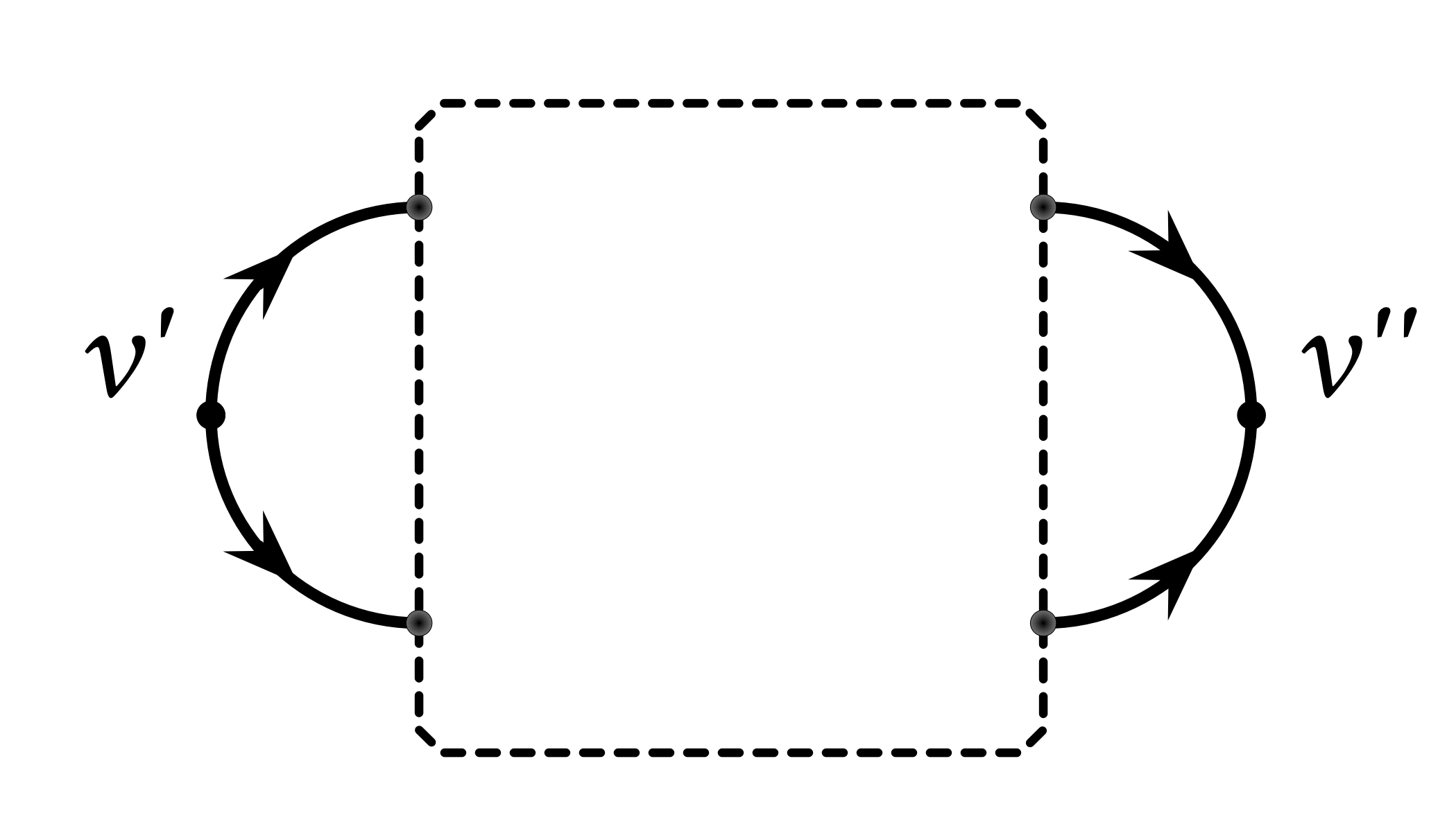
(a) A state in $\Omega_{2}$ with $(=_{2})$’s at $v^{\prime}$ and $v^{\prime\prime}$.

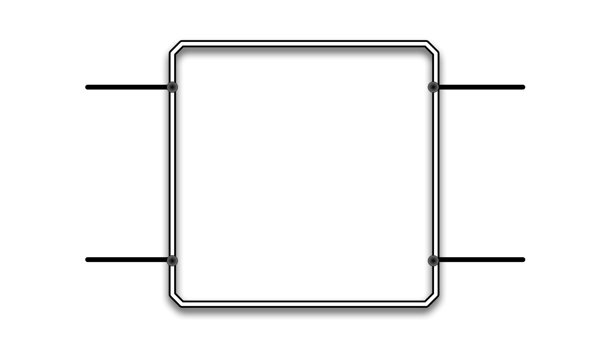
(b) A gadget made by deleting $v^{\prime}$ and $v^{\prime\prime}$.

Figure 6:

For each $\sigma\in\Omega_{2}$, there are exactly two vertices in $V$ satisfying $(=_{2})$. Let $\Omega_{2}^{\{v^{\prime},v^{\prime\prime}\}}\subseteq\Omega_{2}$ be the set of states in which $v^{\prime},v^{\prime\prime}$ are these two vertices. We have $\frac{\mathcal{Z}(\Omega_{2})}{\mathcal{Z}(\Omega_{0})}=\sum_{\{v^{\prime},v^{\prime\prime}\}\ \in\ {V\choose 2}}\frac{\mathcal{Z}(\Omega_{2}^{\{v^{\prime},v^{\prime\prime}\}})}{\mathcal{Z}(\Omega_{0})}$. For any $\sigma\in\Omega_{2}^{\{v^{\prime},v^{\prime\prime}\}}$, the local assignments around $v^{\prime}$ and $v^{\prime\prime}$ must be 00 on one and 11 on the other. An example is in Figure 6(a). If we “delete” $v^{\prime}$ and $v^{\prime\prime}$ as shown in Figure 6(b), we get a 4-ary gadget $g$ on the RHS of $\operatorname{Holant}\left(\neq_{2}|\mathcal{F}_{\leq^{2}}\right)$. Denote the signature matrix of $g$ by $M(g)=\left[\begin{smallmatrix}&&&a^{\prime}\\ &b^{\prime}&c^{\prime}&\\ &c^{\prime}&b^{\prime}&\\ a^{\prime}&&&\end{smallmatrix}\right]$, with the input order being counter-clockwise starting from the upper-left edge. For this gadget $g$ we observe that: the states in $\Omega_{2}^{\{v^{\prime},v^{\prime\prime}\}}$ where edges incident to $v^{\prime}$ (also $v^{\prime\prime}$) take the same value contribute a total weight $(a^{\prime}+a^{\prime})$, i.e. $\mathcal{Z}(\Omega_{2}^{\{v^{\prime},v^{\prime\prime}\}})=2a^{\prime}$; the states in $\Omega_{0}$ where $v^{\prime},v^{\prime\prime}$ satisfy $(\neq_{2})$ have a total weight $\mathcal{Z}(\Omega_{0})=2b^{\prime}+2c^{\prime}$. Note that $\mathcal{F}_{\leq^{2}}\subset\mathcal{F}_{\leq}$. By Theorem 3.1 we know that for gadget $g$, $a^{\prime}\leq b^{\prime}+c^{\prime}$. Therefore, $\frac{\mathcal{Z}(\Omega_{2}^{\{v^{\prime},v^{\prime\prime}\}})}{\mathcal{Z}(\Omega_{0})}\leq 1$. In total, $\frac{\mathcal{Z}(\Omega_{2})}{\mathcal{Z}(\Omega_{0})}\leq\binom{|V|}{2}$. Thus we have the following corollary.

Corollary 4.3.

$\frac{\mathcal{Z}(\Omega_{2})}{\mathcal{Z}(\Omega_{0})}=O(n^{2})$.

Combining Lemma 4.2 and Corollary 4.3, we conclude that $\mathcal{MC}$ is rapidly mixing, and $\Omega_{0}$, the set of valid six-vertex configurations, in total takes a non-negligible proportion in the stationary distribution. As a consequence, we are able to efficiently sample six-vertex configurations according to the Gibbs measure on $\Omega_{0}$, and in the following algorithm we only work with states in $\Omega_{0}$. We design the following algorithm to approximately compute $\operatorname{Holant}\left(\neq_{2}|\mathcal{F}_{\leq^{2}}\right)$ via sampling with the Markov chain $\mathcal{MC}$. As we have argued in Section 3, the partition function of six-vertex models can be viewed as the weighted sum of Eulerian partitions. For a vertex $v\in U$, the ratios among different pairings (, , and ) in weighted Eulerian partitions can be uniquely determined by the ratios among different orientations (represented by $a$, $b$, and $c$) at $v$. As long as the partition function is not zero (this can be easily tested in P), there must be a pairing $\varrho$ showing up at $v$ with probability at least $\frac{1}{3}$ among all three pairings. Therefore, running $\mathcal{MC}$ on $G$, we can approximate, with a sufficient $1/{\rm poly(n)}$ precision, the probability of having $\varrho$ at $v$, denoted by $\Pr_{v}(\varrho)$. Denote by $G_{v,\varrho}$ the signature grid with $v$ being split into $v_{1}$ and $v_{2}$, each assigned a $(\neq_{2})$ and the edges reconnected according to $\varrho$. Write the partition function of $G_{v,\varrho}$ as $Z(G_{v,\varrho})$, we have $\Pr_{v}(\varrho)=w(\varrho)Z(G_{v,\varrho})/Z(G)$ which means $Z(G)=w(\varrho)Z(G_{v,\varrho})/\Pr_{v}(\varrho)$. To approximate $Z(G)$ it suffices to approximate $Z(G_{v,\varrho})$, which can be done by running $\mathcal{MC}$ on $G_{v,\varrho}$ and recursing. Repeating this process for $|U|$ steps we decompose the graph $G$ into the base case, a set of disjoint cycles with even number of vertices, each assigned a $(\neq_{2})$. The partition function of this cycle graph is just $2^{C}$ where $C$ is the number of cycles. By this self-reduction, the partition function for $G$ can be approximated.

Therefore, Theorem 4.1 is proved. Note that for the special case $(1,1,1)$, the FPRAS by Mihail and Winkler is a reduction [MW96] to computing the number of perfect matchings in a bipartite graph. We give a direct algorithm using Markov chain Monte-Carlo.

Remark 4.1.

There is an alternative derivation of a rapidly mixing Markov chain using the notion of “windability” [McQ13, HLZ16], for the purpose of approximating $\operatorname{Holant}\left(\neq_{2}|\mathcal{F}_{\leq^{2}}\right)$. Readers are referred to the Appendix for a proof that signatures in $\mathcal{F}_{\leq^{2}}$ are windable. The mixing rate of that Markov chain can be bounded using similar techniques introduced in this section.

5 Hardness

Theorem 5.1.

If $f\in\mathcal{F}_{>}$, then $\operatorname{Holant}\left(\neq_{2}|f\right)$ does not have an FPRAS unless RP $=$ NP.

Proof.

Let 3-MIS denote the NP-hard problem of computing the cardinality of a maximum independent set in a 3-regular graph [GJS76]. We reduce 3-MIS to approximating $\operatorname{Holant}\left(\neq_{2}|f\right)$. Since $f\in\mathcal{F}_{>}$, all $a,b,c>0$. Since the proof of NP-hardness for $\operatorname{Holant}\left(\neq_{2}|f\right)$ is for general graphs (i.e., not necessarily planar), we can permute the parameters so that $c>a+b$, and normalize $c>b\geq a=1$. Let $\gamma=\frac{c}{a+b}$. Then $\gamma>1$.

Before proving this theorem we briefly state our idea. Denote an instance of 3-MIS by $G=(V,E)$. For any independent set, no two adjacent vertices $u,v\in V$ can both appear. The only possible configurations for $u,v$ in any independent set $S$ are $(u\in S,v\not\in S)$, $(u\not\in S,v\in S)$, and $(u\not\in S,v\not\in S)$. We want to encode this local constraint by a local fragment of $G^{\prime}$ in terms of configurations in the six-vertex model.

(a)

(b)

(c)

Figure 7: A gadget implementing a single edge in independent set.

In Figure 7(a) we show how to implement a toy example—a single edge $\{u,v\}$—by a gadget of the six-vertex model with parameters $(a=1,b=1,c>2)$. Create two vertices, the left one for $u$ and the right one for $v$, and connect them as is shown in Figure 7(a). There are a total of 4 edges. Every 2-in 2-out configuration on the left vertex uniquely extends to a 2-in 2-out configuration on the right, and vice versa. Hence there are a total of 6 valid configurations. When the left vertex has a saddle configuration (in-out-in-out, or its reversal) which has weight $c$, the right must have a non-saddle configuration of weight 1. Figure 7(b) depicts one such configuration; reversing all arrows gives another one having the same weight. Similarly if the right has a saddle configuration (or its reversal) then the left must be a non-saddle. There are two more configurations with two non-saddles (Figure 7(c) and its reversal). This models how two adjacent vertices interact in 3-MIS. We will call the connection pattern described in Figure 7(a) between two sets of 4 dangling edges the four-way connection. Moreover, when $f$ has parameters $c>b\geq a=1$, we can label the input wires so that the 2 saddle configurations of weight $c$ are paired with the 2 non-saddles of weight $b$, and the 2 non-saddle/non-saddle pairs have weight $1$ (by $a=1$).

However, when a vertex in $G$ has more than one neighbors, simply duplicating this elementary implementation will not work, because we cannot make sure that the duplicate copies corresponding to the same vertex $v$ behave consistently. To handle this difficulty, we design a locking gadget (Figure 8) for every $v\in V$ such that the property whether $v$ belongs to an independent set in $G$ is consistently reflected in $G^{\prime}$ in terms of being in a saddle configuration or not. This locking mechanism is enforced in the sense of approximation.

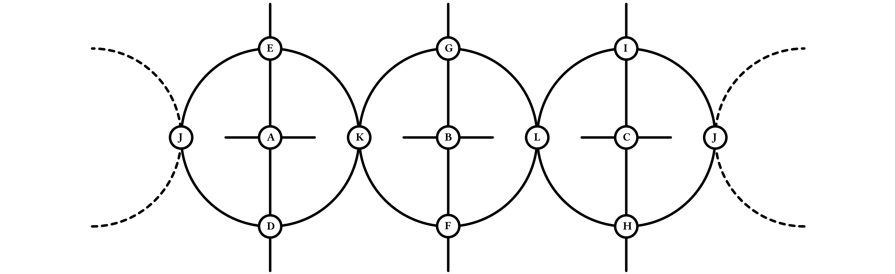
Figure 8: A locking gadget implementing a degree three vertex and its incident edges.

In Figure 8, we identify the leftmost node $J$ with the rightmost node $J$—there are three “circles” in total. The nodes will be replaced by a RHS gadget in $\operatorname{Holant}\left(\neq_{2}|f\right)$. Each circle has 4 dangling edges. The “left circle” has two dangling edges incident to $A$, one incident to $D$, and one incident to $E$. Similarly for the “middle circle” and the “right circle”. Each edge $\{u,v\}$ in $G$ is modeled by a four-way connection of the 4 dangling edges between (one circle of the) gadget for $u$ and that for $v$.

The locking mechanism is to realize the following: when the four dangling edges of one of the 3 circles take a saddle configuration, (either in-out-in-out, or out-in-out-in), the other two circles must also take the identical saddle configuration (in-out-in-out, or out-in-out-in, respectively); when one circle takes any non-saddle configuration, the other two circles can take independently any non-saddle configurations, with no linkage (aside being a non-saddle). This is made possible by chaining, and the guarantee is enforced by approximate counting.

Figure 9: Chaining.

Figure 9 depicts a 2-chain. We place the signature $(\neq_{2})$ on the two degree 2 vertices connecting the two degree 4 vertices, each assigned a copy of $f$. Let $M=M_{x_{i}x_{j},x_{l}x_{k}}(f)=M_{x_{p}x_{q},x_{s}x_{r}}(f)=\left[\begin{smallmatrix}&&&c\\ &a&b&\\ &b&a&\\ c&&&\end{smallmatrix}\right]$. Then the signature $f_{2}$ of this 2-chain gadget is obtained by matrix multiplication $M(f_{2})=M_{x_{i}x_{j},x_{s}x_{r}}(f_{2})=MNM$, where $N=\left[\begin{smallmatrix}&&&1\\ &&1&\\ &1&&\\ 1&&&\end{smallmatrix}\right]$. Thus $M(f_{2})=\left[\begin{smallmatrix}&&&c_{2}\\ &a_{2}&b_{2}&\\ &b_{2}&a_{2}&\\ c_{2}&&&\end{smallmatrix}\right]=\left[\begin{smallmatrix}&&&c^{2}\\ &2ab&a^{2}+b^{2}&\\ &a^{2}+b^{2}&2ab&\\ c^{2}&&&\end{smallmatrix}\right]$, where $c_{2}=c^{2}$, $a_{2}+b_{2}=(a+b)^{2}$. Thus $c_{2}>a_{2}+b_{2}$, and $\gamma_{2}:=\frac{c_{2}}{a_{2}+b_{2}}=\left(\frac{c}{a+b}\right)^{2}=\gamma^{2}$.

This can be generalized to a $k$-chain, which connects $k$ vertices with signature $f$ by $k-1$ copies of $N$, such that $c_{k}=c^{k},a_{k}+b_{k}=(a+b)^{k},\gamma_{k}=\gamma^{k}$. Notice that when $c>a+b$, the ratio $\frac{c}{a+b}$ can be amplified exponentially in $k$ in a $k$-chain. Therefore, by a chain of polynomially bounded size we can ensure the undesirable configurations are negligible—the gadget is locked into the only two complementary configurations which $c$ represents. It can be verified that $b_{k}=(\mu^{k}+\nu^{k})/2\geq a_{k}=(\mu^{k}-\nu^{k})/2\geq 1$, where $\mu=a+b$ and $\nu=b-a$. We can “normalize” a $k$-chain by dividing $a_{k}$, so that its parameters are $\tilde{c}_{k}=c^{k}/a_{k}>\tilde{b}_{k}=b_{k}/a_{k}\geq\tilde{a}_{k}=1$.

To reduce the problem 3-MIS to approximating $\operatorname{Holant}\left(\neq_{2}|f\right)$, let $\kappa>\lambda\geq 1$ be two constants whose magnitude will later become clear. For each 3-MIS instance $G=(V,E)$ with $|V|=n$, we construct a graph $G^{\prime}$ where a gadget in Figure 8 is created for each $v\in V$, and a four-way connection is made for every $\{u,v\}\in E$, on the dangling edges between two circles corresponding to $\{u,v\}$ as in Figure 7(a). For each gadget in Figure 8, each of the nodes $A,B,C$ is replaced by a normalized $\lambda n$-chain to boost the ratio of the saddle configuration over other configurations; each of the nodes $D,F,H$ is replaced by a $\kappa n^{2}$-chain to lock in the configuration “all arrows pointing up and right” and its reversal; each of the nodes $E,G,I$ is also replaced by a $\kappa n^{2}$-chain to lock in the configuration “all arrows pointing down and right” and its reversal (these configurations at $D,F,H$, and at $E,G,I$ respectively, will be called locking configurations); at each of $J,K,L$, we just put $f$ in which the maximum weight of a configuration over the minimum is a constant $\frac{c}{\min\{a,b\}}=c$. Note that the signature in Figure 9 has the dominating entry at 0011 and 1100. Since our graph $G^{\prime}$ does not need to be planar, we can reorder the 4 external edges arbitrarily. In particular, for $A,B,C$ the dominating entry $\tilde{c}_{\lambda n}$ is in the saddle 0101 and 1010 positions, as depicted in Figure 8. Similarly the 4 external edges of $D,F,H$ and $E,G,I$ are also properly reordered, from the order given in Figure 9, as an $\lambda n$-chain to achieve the proper locking configurations.

Next we argue that the maximum size $s$ of independent sets in $G$ can be recovered from an approximate solution to $\operatorname{Holant}\left(G^{\prime};\neq_{2}|f\right)$.

Given an independent set $S\subset V$ of size $s$, we show there is a valid configuration (at the granularity of nodes and edges shown in Figure 8) of weight $\geq c^{6\kappa n^{3}}\left(\tilde{c}_{\lambda n}\tilde{b}_{\lambda n}\right)^{3s}$. For any vertex $v\in S$ we set the following configuration for its locking gadget: set each of 3 nodes $A,B,C$ to the same saddle configuration in-out-in-out cyclically starting from the upper edge—each has weight $\tilde{c}_{\lambda n}$; set each of 3 nodes $D,F,H$ to the same out-out-in-in locking configuration (clockwise) cyclically starting from the upper edge—each has weight $c^{\kappa n^{2}}$; set each of 3 nodes $E,G,I$ to the same in-out-out-in locking configuration (clockwise) cyclically starting from the upper edge—each also has weight $c^{\kappa n^{2}}$; set each of 3 nodes $J,K,L$ to the same configuration “two in from the left and two out to the right”, which has a non-zero weight $\geq 1$. For any vertex $v\not\in S$ we set the following configuration for its locking gadget: All $D,F,H,E,G,I$ will be in some locking configurations. Consider any of the 3 circles in the gadget, for example the circle formed by $A,D,E,J,K$. The node $A$ is involved in a four-way connection to another circle belonging to a gadget for some vertex $u$. If $u\in S$, the assigned configuration just defined at $u$ forces a non-saddle configuration here; more specifically the horizontal two dangling edges at $A$ must either both point right or both point left, and the upper edge $\hat{e}$ of $E$ and lower edge $\underline{e}$ of $D$ must either both point up or both point down. Regardless of which of the two assignments for $\hat{e}$ and $\underline{e}$ we can assign a locking configuration for $E$ and $D$ so that the upper and lower edges of $A$ are either both point up or both point down. Note that in either case, the left two edges of $K$ are one-in-one-out; similarly the right two edges of $J$ are also one-in-one-out (this allows “freedom” between the 3 circles where each of $J$, $K$, $L$ can take a nonzero weight $\geq 1$). Continuing at the circle $A,D,E,J,K$, if $u\not\in S$, then we will pick an arbitrary non-saddle to non-saddle configuration in the 4-way connection for $\{u,v\}$. These can all be extended to a valid configuration at $A,D,E$ such that the configuration at $A$ is non-saddle having weight $\geq 1$, the configurations at $D$ and $E$ are locking, and the right two edges of $J$ and the left two edges of $K$ are both one-in-one-out. The weight at $D$ and $E$ are still $c^{\kappa n^{2}}$. Because $J$ and $K$ each has one-in-one-out from within the side of the circle, the 3 circles can be assigned independently from each other. This allows us to handle the situation where, for the same $v\not\in S$, some edge $\{v,u\}$ connects to $u\in S$ and some edge $\{v,u^{\prime}\}$ connects to $u^{\prime}\not\in S$.

We have defined a valid configuration, and it has weight $\geq\prod_{v\in V}c^{6\kappa n^{2}}\prod_{v\in S}\left(\tilde{c}_{\lambda n}\tilde{b}_{\lambda n}\right)^{3}=c^{6\kappa n^{3}}\left(\tilde{c}_{\lambda n}\tilde{b}_{\lambda n}\right)^{3s}$, where $6$ comes from the 6 locking nodes $D,E,F,G,H,I$ in each locking gadget. (Omitted factors are all $\geq 1$.)

Next we show the weighted sum of all configurations is smaller than $c^{6\kappa n^{3}}\left(\tilde{c}_{\lambda n}\tilde{b}_{\lambda n}\right)^{3(s+1)}$. First we bound $W_{\rm lock}$, the sum of weights for configurations where all nodes labeled $D,E,F,G,H,I$ are locked. Consider any circle such as the one labeled $A,D,E,J,K$ for any $v\in V$. It is involved in a four-way connection with another such circle for a vertex $u\in V$, say $A^{\prime},D^{\prime},E^{\prime},J^{\prime},K^{\prime}$, where $\{u,v\}\in E$. That $D$ is locked forces that the upper and lower edges of $D$ are to be consistently oriented, i.e., both up or both down. Similarly, consistency holds at $E$, $D^{\prime}$ and $E^{\prime}$. Thus the four-way connection forces that there can be at most one of $A$ and $A^{\prime}$ is in a saddle configuration. Furthermore, if $A$ is in a particular saddle configuration, say in-out-in-out starting from the upper edge, both upper and lower edges of $D$ must point up, and both upper and lower edges of $E$ must point down, and then both right edges of $D$ and $E$ must point right, causing the left two edges of $K$ point in, and thus the right two edges of $K$ point out. This forces both $F$ and $G$ to take exactly the same locked configurations of $D$ and $E$ respectively, whch forces $B$ to be in exactly the same saddle configuration as $A$. Similarly so is $C$. We conclude that when all nodes labeled $D,E,F,G,H,I$ are locked, for any $v\in V$, if any of its $A,B,C$ is in a saddle configuration, then all 3 are in exactly the same saddle configuration, and none of $A^{\prime},B^{\prime},C^{\prime}$ for $u\in V$ is a saddle, if $\{u,v\}\in E$. In particular, there can be at most $3s$ many saddles among $A,B,C$’s in $G^{\prime}$. If $0\leq i\leq s$ is the number of $\{A,B,C\}$’s being in saddle, their weight is $\left(\tilde{c}_{\lambda n}\right)^{3i}$, and their corresponding non-saddles in respective four-way connections must take weight $\left(\tilde{b}_{\lambda n}\right)^{3i}$. Those $(3n-6i)/2$ pairwise four-way connections between two non-saddles have weight $\tilde{a}_{\lambda n}=1$. Note that, if any of those non-saddles were to take weight $\tilde{b}_{\lambda n}$, then the corresponding paired node in its four-way connection must be in saddle, a contradiction.

It follows that

$$W_{\rm lock}\leq 2^{6n}\left(c^{\kappa n^{2}}\right)^{6n}\sum_{i=0}^{s}\binom{n}{i}\left(\tilde{c}_{\lambda n}\tilde{b}_{\lambda n}\right)^{3i}c^{3n}\leq 2^{7n}c^{6\kappa n^{3}+3n}\left(\tilde{c}_{\lambda n}\tilde{b}_{\lambda n}\right)^{3s},$$

where each locked node $D,E,F,G,H,I$ has 2 possible locking configurations each with weight $c^{\kappa n^{2}}$, and given a particular assignment of $6n$ locking configurations, there can be at most $s$ batches of $A,B,C$’s in saddle configurations (same for each batch and determined by the locks) with weight $\tilde{c}_{\lambda n}$. Hence $W_{\rm lock}<\frac{1}{2}c^{6\kappa n^{3}}\left(\tilde{c}_{\lambda n}\tilde{b}_{\lambda n}\right)^{3(s+1)}$, when $\lambda\geq 1$ is large.

It remains to upper-bound the weighted sum of configurations where there is at least one gadget with some lock broken. This quantity is bounded by

$$\sum_{i=0}^{6n-1}\binom{6n}{i}c^{i\kappa n^{2}}(a+b)^{(6n-i)\kappa n^{2}}6^{6n}\left[2\left(\tilde{c}_{\lambda n}+\tilde{b}_{\lambda n}+1\right)\right]^{3n}[2(a+b+c)]^{3n}$$

$$\leq\; 2^{\Theta(n)}(a+b)^{6\kappa n^{3}}\left(\frac{c}{a+b}\right)^{(6n-1)\kappa n^{2}}\left[\tilde{c}_{\lambda n}+\tilde{b}_{\lambda n}+1\right]^{3n}[a+b+c]^{3n}$$

$$\leq\; 2^{\Theta(n)}[\Theta(1)]^{\lambda n^{2}}c^{6\kappa n^{3}}\frac{1}{c^{\kappa n^{2}}}(a+b)^{\kappa n^{2}}$$

$$\leq\; 2^{\Theta(n)}[\Theta(1)]^{\lambda n^{2}}c^{6\kappa n^{3}}\frac{1}{\gamma^{\kappa n^{2}}},$$

which is $<\frac{1}{2}c^{6\kappa n^{3}}$ when $\kappa\gg\lambda\geq 1$ is large. ∎

6 Open problems

The main open problem on the approximate complexity of the six-vertex model is in the white region. The finer classification of the approximate complexity for the planar case is also open. Approximating $T(G;3,3)$ is #BIS-hard for general graphs [GJ12]. On planar graphs, $T(G;3,3)$ is equivalent to the six-vertex model at $(1,1,2)$ where the approximation complexity for planar graphs is unknown.

Appendix

The near-assignments Markov chain for windable functions is proposed by Colin McQuillan in [McQ13] and further analyzed in [HLZ16]. In the following we present the definition of windable functions given in the latter and show that signatures in $\mathcal{F}_{\leq^{2}}$ are all windable. This leads to an alternative derivation of a rapidly mixing Markov chain, and based on this chain the techniques introduced in Section 4 can be adapted to give a FPRAS for $\operatorname{Holant}\left(\neq_{2}|\mathcal{F}_{\leq^{2}}\right)$.

Definition.

For any finite set $J$ and any configuration $x\in\{0,1\}^{J}$, define $\mathcal{M}_{x}$ to be the set of partitions of $\{i\ |\ x_{i}=1\}$ into pairs and at most one singleton. A signature $f:\{0,1\}^{J}\rightarrow\mathbb{R^{+}}$ is windable if there exist values $B(x,y,M)\geq 0$ for any two distinct $x,y\in\{0,1\}^{J}$ and all $M\in\mathcal{M}_{x\oplus y}$, such that:

1. $f(x)f(y)=\sum_{M\in\mathcal{M}_{x\oplus y}}B(x,y,M)$ for all distinct $x,y\in\{0,1\}^{J}$, and

2. $B(x,y,M)=B(x\oplus S,y\oplus S,M)$ for all distinct $x,y\in\{0,1\}^{J}$ and all $S\in M\in\mathcal{M}_{x\oplus y}$.

Here $x\oplus S$ denotes the vector obtained by changing $x_{i}$ to $1-x_{i}$ for the one or two elements $i$ in $S$.

The signature $(\neq_{2})$ is shown to be windable in [McQ13]. We show that signatures in $\mathcal{F}_{\leq^{2}}$ are all windable.

Lemma.

For any nonnegative real numbers $a$, $b$, and $c$, the function $f$ with signature matrix $M(f)=\left[\begin{smallmatrix}&&&a\\ &b&c&\\ &c&b&\\ a&&&\end{smallmatrix}\right]$ is windable if and only if $a^{2}\leq b^{2}+c^{2}$, $b^{2}\leq a^{2}+c^{2}$, and $c^{2}\leq a^{2}+b^{2}$.

Proof.

According to the definition, we need to verify when there exist values $B(x,y,M)\geq 0$ for all distinct $x,y\in\{0,1\}^{4}$ and all $M\in\mathcal{M}_{x\oplus y}$ that satisfy the two conditions. Let $\operatorname{Hw}(x)$ denote the Hamming weight of a 0-1 vector $x$. We make the following observations:

1. Since $f$ only takes nonzero values on inputs of Hamming weight ($\operatorname{Hw}$) 2, by condition I we must have $B(x,y,M)=0$ for all $M\in\mathcal{M}_{x\oplus y}$, if $\operatorname{Hw}(x)\neq 2$ or $\operatorname{Hw}(y)\neq 2$.

2. For any distinct $x,y$ with $\operatorname{Hw}(x)=\operatorname{Hw}(y)=2$, if $y\neq\bar{x}$ then $|\mathcal{M}_{x\oplus y}|=1$. Denote this unique partition by $M$, by condition II we have $B(x,y,M)=B(y,x,M)$.

3. For any $x,y$ with $\operatorname{Hw}(x)=\operatorname{Hw}(y)=2$, if $y=\bar{x}$ then

   $$\mathcal{M}_{x\oplus y}=\{\{\{1,2\},\{3,4\}\},\{\{1,3\},\{2,4\}\},\{\{1,4\},\{2,3\}\}\}$$

   and we still have $B(x,y,M)=B(y,x,M)$ for any $M\in\mathcal{M}_{x\oplus y}$.

4. B(0011, 1100, {{1,2}, {3,4}}) = B(0110, 1001, {{1,4}, {2,3}}) = B(0101, 1010, {{1,3}, {2,4}}) = 0; otherwise, by condition II and condition I we would have $f(0000)f(1111)\neq 0$, a contradiction.

5. By condition II,

   • $B(0011,1100,\{\{1,3\},\{2,4\}\})=B(0110,1001,\{\{1,3\},\{2,4\}\})$;

   • $B(0011,1100,\{\{1,4\},\{2,3\}\})=B(0101,1010,\{\{1,4\},\{2,3\}\})$;

   • $B(0110,1001,\{\{1,2\},\{3,4\}\})=B(0101,1010,\{\{1,2\},\{3,4\}\})$.

   Denote them by $X$, $Y$, and $Z$, respectively.

Combining these observations, we are left with 15 variables and 15 equations:

$$\left\{\begin{array}[]{ll}B(0011,0110,\{\{2,4\}\})=f(0011)f(0110)=ab,&B(0110,0101,\{\{3,4\}\})=f(0110)f(0101)=bc,\\ B(0011,1001,\{\{1,3\}\})=f(0011)f(1001)=ab,&B(0110,1010,\{\{1,2\}\})=f(0110)f(1010)=bc,\\ B(0011,0101,\{\{2,3\}\})=f(0011)f(0101)=ac,&B(1001,0101,\{\{1,2\}\})=f(1001)f(0101)=bc,\\ B(0011,1010,\{\{1,4\}\})=f(0011)f(1010)=ac,&B(1001,1010,\{\{3,4\}\})=f(1001)f(1010)=bc,\\ B(1100,0110,\{\{1,3\}\})=f(1100)f(0110)=ab,&X+Y=f(0011)f(1100)=a^{2},\\ B(1100,1001,\{\{2,4\}\})=f(1100)f(1001)=ab,&X+Z=f(0110)f(1001)=b^{2},\\ B(1100,0101,\{\{1,4\}\})=f(1100)f(0101)=ac,&Y+Z=f(0101)f(1010)=c^{2},\\ B(1100,1010,\{\{2,3\}\})=f(1100)f(1010)=ac.\\ \end{array}\right.$$

(Here the $B$’s and $X,Y,Z$ are variables.) The system of equations has nonnegative solutions if and only if the set of the last three equations has. This holds if and only if $a^{2}\leq b^{2}+c^{2}$, $b^{2}\leq a^{2}+c^{2}$, and $c^{2}\leq a^{2}+b^{2}$. ∎

References

- [Bax82] R. J. Baxter. Exactly Solved Models in Statistical Mechanics. Academic Press Inc., San Diego, CA, USA, 1982.
- [CFS17] Jin-Yi Cai, Zhiguo Fu, and Shuai Shao. A complexity trichotomy for the six-vertex model. CoRR, abs/1704.01657, 2017.
- [DFK91] Martin Dyer, Alan Frieze, and Ravi Kannan. A random polynomial-time algorithm for approximating the volume of convex bodies. J. ACM, 38(1):1–17, January 1991.
- [DGGJ04] Martin Dyer, Leslie Ann Goldberg, Catherine Greenhill, and Mark Jerrum. The relative complexity of approximate counting problems. Algorithmica, 38(3):471–500, Mar 2004.
- [EMM11] Joanna A. Ellis-Monaghan and Criel Merino. Graph polynomials and their applications I: The Tutte polynomial. In Matthias Dehmer, editor, Structural Analysis of Complex Networks, pages 219–255. Birkhäuser Boston, Boston, 2011.
- [FW70] Chungpeng Fan and F. Y. Wu. General lattice model of phase transitions. Phys. Rev. B, 2:723–733, Aug 1970.
- [GJ12] Leslie Ann Goldberg and Mark Jerrum. Approximating the partition function of the ferromagnetic Potts model. J. ACM, 59(5):25:1–25:31, November 2012.
- [GJS76] M.R. Garey, D.S. Johnson, and L. Stockmeyer. Some simplified NP-complete graph problems. Theoretical Computer Science, 1(3):237 – 267, 1976.
- [GMP04] Leslie Ann Goldberg, Russell Martin, and Mike Paterson. Random sampling of 3-colorings in . Random Structures & Algorithms, 24(3):279–302, 2004.
- [GW13] Heng Guo and Tyson Williams. The complexity of planar Boolean #CSP with complex weights. In Proceedings of the 40th International Colloquium on Automata, Languages, and Programming, ICALP ’13, pages 516–527, Berlin, Heidelberg, 2013. Springer Berlin Heidelberg.
- [HL16] Sangxia Huang and Pinyan Lu. A dichotomy for real weighted Holant problems. Computational Complexity, 25(1):255–304, March 2016.
- [HLZ16] Lingxiao Huang, Pinyan Lu, and Chihao Zhang. Canonical paths for MCMC: From art to science. In Proceedings of the Twenty-seventh Annual ACM-SIAM Symposium on Discrete Algorithms, SODA ’16, pages 514–527, Philadelphia, PA, USA, 2016. Society for Industrial and Applied Mathematics.
- [Jae90] F. Jaeger. On transition polynomials of 4-regular graphs. In Geňa Hahn, Gert Sabidussi, and Robert E. Woodrow, editors, Cycles and Rays, pages 123–150. Springer Netherlands, Dordrecht, 1990.
- [Jer03] Mark Jerrum. Counting, Sampling and Integrating: Algorithm and Complexity. Birkhäuser, Basel, 2003.
- [JS89] Mark Jerrum and Alistair Sinclair. Approximating the permanent. SIAM Journal on Computing, 18(6):1149–1178, 1989.
- [JSV04] Mark Jerrum, Alistair Sinclair, and Eric Vigoda. A polynomial-time approximation algorithm for the permanent of a matrix with nonnegative entries. J. ACM, 51(4):671–697, July 2004.
- [JVV86] Mark R. Jerrum, Leslie G. Valiant, and Vijay V. Vazirani. Random generation of combinatorial structures from a uniform distribution. Theoretical Computer Science, 43(Supplement C):169 – 188, 1986.
- [KL83] Richard M. Karp and Michael Luby. Monte-Carlo algorithms for enumeration and reliability problems. In Proceedings of the 24th Annual Symposium on Foundations of Computer Science, SFCS ’83, pages 56–64, Washington, DC, USA, 1983. IEEE Computer Society.
- [Kup96] Greg Kuperberg. Another proof of the alternative-sign matrix conjecture. International Mathematics Research Notices, 1996(3):139–150, 1996.
- [Lie67a] Elliott H. Lieb. Exact solution of the model of an antiferroelectric. Phys. Rev. Lett., 18:1046–1048, Jun 1967.
- [Lie67b] Elliott H. Lieb. Exact solution of the two-dimensional slater KDP model of a ferroelectric. Phys. Rev. Lett., 19:108–110, Jul 1967.
- [Lie67c] Elliott H. Lieb. Residual entropy of square ice. Phys. Rev., 162:162–172, Oct 1967.
- [LRS01] Michael Luby, Dana Randall, and Alistair Sinclair. Markov chain algorithms for planar lattice structures. SIAM Journal on Computing, 31(1):167–192, 2001.
- [McQ13] Colin McQuillan. Approximating Holant problems by winding. CoRR, abs/1301.2880, 2013.
- [MW96] M. Mihail and P. Winkler. On the number of eulerian orientations of a graph. Algorithmica, 16(4):402–414, Oct 1996.
- [Pau35] Linus Pauling. The structure and entropy of ice and of other crystals with some randomness of atomic arrangement. Journal of the American Chemical Society, 57(12):2680–2684, 1935.
- [RT00] Dana Randall and Prasad Tetali. Analyzing Glauber dynamics by comparison of Markov chains. Journal of Mathematical Physics, 41(3):1598–1615, 2000.
- [Sin92] Alistair Sinclair. Improved bounds for mixing rates of Markov chains and multicommodity flow. Combinatorics, Probability and Computing, 1:351–370, 1992.
- [Sla41] J. C. Slater. Theory of the transition in KH2PO4. The Journal of Chemical Physics, 9(1):16–33, 1941.
- [Sut67] Bill Sutherland. Exact solution of a two-dimensional model for hydrogen-bonded crystals. Phys. Rev. Lett., 19:103–104, Jul 1967.
- [Tut54] W. T. Tutte. A contribution to the theory of chromatic polynomials. Canad. J. Math., 6(0):80–91, January 1954.
- [Ver88] Michel Las Vergnas. On the evaluation at (3, 3) of the Tutte polynomial of a graph. Journal of Combinatorial Theory, Series B, 45(3):367 – 372, 1988.
- [Zei96] Doron Zeilberger. Proof of the alternating sign matrix conjecture. Electronic Journal of Combinatorics, 3(2), 1996.