Relaxation in self-gravitating systems

Abstract

The long timescale evolution of a self-gravitating system is generically driven by two-body encounters. In many cases, the motion of the particles is primarily governed by the mean field potential. When this potential is integrable, particles move on nearly fixed orbits, which can be described in terms of angle-action variables. The mean field potential drives fast orbital motions (angles) whose associated orbits (actions) are adiabatically conserved on short dynamical timescales. The long-term stochastic evolution of the actions is driven by the potential fluctuations around the mean field and in particular by “resonant two-body encounters”, for which the angular frequencies of two particles are in resonance. We show that the stochastic gravitational fluctuations acting on the particles can generically be described by a correlated Gaussian noise. Using this approach, the so-called $\eta$-formalism, we derive a diffusion equation for the actions in the test particle limit. We show that in the appropriate limits, this diffusion equation is equivalent to the inhomogeneous Balescu-Lenard and Landau equations. This approach provides a new view of the resonant diffusion processes associated with long-term orbital distortions. Finally, by investigating the example of the Hamiltonian Mean Field Model, we show how the present method generically allows for alternative calculations of the long-term diffusion coefficients in inhomogeneous systems.

1 Introduction

The long-term evolution of self-gravitating systems has been a long-standing subject of interest in many astrophysical contexts. Long-range interacting systems such as stellar disks, globular clusters, and nuclear star clusters, share indeed some fundamental similarities. First, they are inhomogeneous systems: the dynamics of their individual components is intricate. Second, owing to their relatively short dynamical timescales compared to their age, these systems are also generically dynamically relaxed so that their mean field distribution may be assumed to be quasi-stationary. Third, these systems are also perturbed, either via external sources (e.g., satellite infall in stellar disks or tidal forcing via an external potential) or via self-induced fluctuations (e.g., finite${-N}$ effects). Finally, these systems are self-gravitating so that any perturbation, either internal or external, can be amplified. These various effects contribute to the long-term dynamics of self-gravitating systems.

A first source of diffusion is external potential fluctuations. Neglecting collective effects (i.e. the ability of the system to respond to perturbations), Binney & Lacey (1988) computed the first- and second-order diffusion coefficients in orbital space. Weinberg (1993, 2001a, 2001b) emphasized the importance of collective effects and studied the impact of the properties of the noise processes in shaping the diffusion coefficients. Pichon & Aubert (2006) presented a time-decoupling approach to solve the collisionless Boltzmann equation in the presence of external perturbations, and studied the long-term evolution dark matter halos. A similar method was presented in Fouvry et al. (2015a) in the context of stellar disks. The effects of stochastic forces on long-range interacting systems were also investigated in Chavanis (2012a); Nardini et al. (2012).

Even without external perturbations, isolated self-gravitating systems can undergo a long-term diffusion caused by potential fluctuations arising from their finite number of particles. Early studies of the long-term effects of self-induced internal potential fluctuations (e.g., Chandrasekhar, 1942; Spitzer, 1987) relied essentially on various simplifying assumptions (see e.g., Nelson & Tremaine, 1999; Bar-Or et al., 2013; Chavanis, 2013; Heyvaerts et al., 2017, for a detailed historical account). First, the system was assumed to be spatially infinite and homogeneous so that individual trajectories become simple straight lines. Second, stellar encounters are assumed to be instantaneous and uncorrelated so that the stochastic evolution of the stellar velocities can be assumed to be a Markov process. Third, changes in velocity are assumed to result from a sequence of many small changes so that, by the central limit theorem, the distribution of velocity changes can be assumed to be Gaussian. Finally, collective effects (i.e. the ability of the system to amplify perturbations via its self-gravity) were neglected. Recent progresses in the kinetic theory of inhomogeneous self-gravitating systems have been able to relax some of these assumptions. These developments rely on the use of angle-action coordinates (e.g., Binney & Tremaine, 2008) to account for the intricate trajectories, and the use of linear response theory and the associated matrix method (Kalnajs, 1976) to account for self-gravity (see Section 5.3. in Binney & Tremaine, 2008). This led to the so-called inhomogeneous Landau equation (Polyachenko & Shukhman, 1982; Chavanis, 2013) when collective effects are neglected, and the inhomogeneous Balescu-Lenard (BL) equation (Luciani & Pellat, 1987; Mynick, 1988; Heyvaerts, 2010; Chavanis, 2012b) when collective effects are accounted for. Various derivations of these kinetic equations were proposed in the literature. Luciani & Pellat (1987); Chavanis (2012b) obtained the inhomogeneous BL equation starting from the Klimontovich equation (Klimontovich, 1967). The same kinetic equations were derived from the direct solution of the two first equations of the BBGKY equations truncated at the order ${1/N}$ by Heyvaerts (2010) and by direct computation of the first- and second-order diffusion coefficients following the Fokker-Planck approach (Mynick, 1988; Chavanis, 2012b; Heyvaerts et al., 2017).

Subsequent studies illustrated the relevance of these kinetic theories to various astrophysical systems.  Fouvry et al. (2015b); Fouvry et al. (2015c, 2017b), applied the BL equation to razor-thin and thickened stellar disks. These studies emphasized in particular the importance of collective effects to hasten the (resonant) relaxation of dynamically cold self-gravitating systems. The same kinetic equation was also specialized to quasi-Keplerian (degenerate) systems, such as galactic centers, in Sridhar & Touma (2016a, b, 2017); Fouvry et al. (2017c, a). Finally, Benetti & Marcos (2017) used the same framework to compute the diffusion coefficients of the one-dimensional inhomogeneous Hamiltonian mean field (HMF) model (Antoni & Ruffo, 1995), both with and without collective effects. In Section 8, we will consider the same HMF model to illustrate the new paradigm introduced in the present work. In all these contexts, the inhomogeneous BL equation was put forward as a powerful new kinetic equation allowing for detailed and quantitative descriptions of the long-term self-induced evolution of self-gravitating systems. This framework offers in particular alternative probes of complex long-term regimes in complement to traditional $N$-body methods. Such kinetic theories may indeed be applied to a wide range of astrophysical scales from the cusp-core transformation of dark halos, through the processes of radial migration or thickening in stellar disks, all the way down to the resonant relaxation of galactic nuclei (Rauch & Tremaine, 1996; Hopman & Alexander, 2006; Bar-Or & Alexander, 2016).

The inhomogeneous Landau equation and the more general inhomogeneous BL equation are, to date, the most general diffusion equations to describe the long-term evolution of inhomogeneous self-gravitating multi-component systems. Nevertheless, in practice, calculating the associated diffusion coefficients is not an easy task. The diffusion coefficients are expressed as an infinite sum over resonances and involve an integral over action space. As a result, in many systems these diffusion coefficients have to be evaluated numerically to some finite order. An alternative approach was put forward in Bar-Or & Alexander (2014) to study the resonant relaxation of stars around a massive black hole, in a regime where general relativistic effects play an important role. Bar-Or & Alexander (2014) introduced the $\eta$-formalism (see the review by Alexander, 2015), in which the intricate orbital motion of a test star is perturbed by an external stochastic noise acting on it. The orbital evolution of the test star is then described by a Fokker-Planck (FP) equation where the diffusion coefficients depend on the power density of the noise. In fact, as we will show here, these diffusion coefficients are equivalent to the Landau or BL ones in the appropriate regime. Even within this approach, the associated diffusion coefficients remain hard to evaluate, and the difficulty lies here in the evaluation of the noise term. However, because this noise term has a physical meaning, it can be approximated via considerations on the typical timescales of the system. This approach was used in Bar-Or & Alexander (2014) to explain the so-called “Schwarzschild Barrier”, which was observed in $N$-body simulations (Merritt et al., 2011). The same method was also used in Bar-Or & Alexander (2016) to estimate the rate with which compact objects, like stellar black holes, are driven to strongly interact with a central massive black hole to produce gravitational waves.

In the present paper, we revisit these different kinetic equations (for both external and self-induced evolution), and emphasize their strong connections. To do so, we follow and generalize the $\eta$-formalism. Our method underlines especially the importance of the stochasticity of potential fluctuations in sourcing the long-term diffusion of self-gravitating systems. We show in particular how both external and self-induced potential fluctuations can be reconciled within the same framework. The paper is organized as follows. In Section 2, we present the key ingredients of the $\eta$-formalism. In Section 3, we derive the inhomogeneous diffusion coefficients describing the orbital diffusion of a test particle induced by an external stochastic bath. In Section 4, we show how these approaches allow for the explicit and exact recovery of the inhomogeneous Landau and BL diffusion coefficients. In Section 5, we briefly recover the so-called friction force by polarization by accounting for the back-reaction of the test particle on the bath particles, an essential component of any self-consistent diffusion equation. In Section 7, we detail how the external dressed diffusion equation from Binney & Lacey (1988); Weinberg (2001a) may also be recovered.In Section 8, we demonstrate and emphasize the practical relevance of this method by recovering the inhomogeneous diffusion coefficients of the HMF model. Finally, we summarize our results in Section 9.

2 Stochastic Hamiltonian

In this first section, we consider the long-term evolution of a test particle embedded in an external “bath” of ${N\gg 1}$ particles. As discussed later, here, external means that there are no back-reactions of the test particle onto the evolution of the bath particles. It is a completely deterministic system, that is the evolution of the test particle depends only on the positions ${\mathbf{x}_{i}}$ and velocities ${\mathbf{v}_{i}}$ of all the ${N}$ bath particles at some time $t_{0}$. Nevertheless, the complex motion of the bath particles exerts a force on the test particle that in the large $N$ limit can be regarded as a random process. This is one of the key considerations of the upcoming calculations. As a result, the potential induced by the bath, which depends on the exact motion of the bath particles, can be replaced by a stochastic potential characterized by its statistical correlations. The motion of the test particle may then be described by a stochastic Hamiltonian.

First, let us specify the properties of the considered bath. We assume that it takes the form of a generic $N$-body system governed by a long-range pairwise interaction potential ${\psi(\mathbf{x},{\mathbf{x}^{\prime}})\propto 1/{|\mathbf{x}-{\mathbf{x}^{\prime}}|}^{\alpha}}$. This interaction is taken to be long-range, so that ${\alpha\leq d}$, with $d$ the dimensionality of the system (e.g, Campa et al., 2009). In the gravitational context, one has ${\psi(\mathbf{x},{\mathbf{x}^{\prime}})=-G/|\mathbf{x}-{\mathbf{x}^{\prime}}|}$, and therefore ${\alpha=1}$. The Hamiltonian driving the evolution of the bath particles is then given by

$$H_{\mathrm{b}}(\{\mathbf{x}_{i}\},\{\mathbf{p}_{i}\})=\sum_{i=1}^{N}\frac{{|\mathbf{p}_{i}|}^{2}}{2m_{i}}\,\,+\!\!\sum_{1\leq i<j\leq N}\!\!\!\!\!\!m_{i}\,m_{j}\,\psi(\mathbf{x}_{i},\mathbf{x}_{j})+\sum_{i=1}^{N}m_{i}\,U_{\mathrm{ext}}(\mathbf{x}_{i}),$$ (1)

where $m_{i}$ is the mass of the $i$-th bath particle. The location in phase space of this particle at time $t$ is given by the canonical coordinates ${(\mathbf{x}_{i},\mathbf{p}_{i}=m_{i}\mathbf{v}_{i})}$. In addition to pairwise interactions, the Hamiltonian in equation (1) can also involve an external stationary time-independent potential, $U_{\rm ext}$. For simplicity, we will assume that the bath is of total mass $M$, and that all the bath particles have the same individual mass ${m_{\mathrm{b}}=M/N}$.

In the present work, we are interested in the long-term behavior of one given test particle of mass $m_{\mathrm{t}}$, orbiting in the potential induced by the bath. The evolution of this test particle is governed by the time-dependent specific Hamiltonian

$$H_{\mathrm{t}}(\mathbf{v},\mathbf{x},t)=\frac{{|\mathbf{v}|}^{2}}{2}+\sum_{n=1}^{N}m_{\mathrm{b}}\,\psi(\mathbf{x},\mathbf{x}_{n}(t))+U_{\mathrm{ext}}(\mathbf{x}),$$ (2)

where the location of the test particle in phase space is given by ${(\mathbf{x},\mathbf{v})}$, and the sum over $n$ runs over all the bath particles. By averaging the Hamiltonian over all possible realizations of the bath, we obtain the mean Hamiltonian of the test particle

$$H_{0}(\mathbf{x},\mathbf{v},t)=\frac{{|\mathbf{v}|}^{2}}{2}+\!\!\int\!\!\mathrm{d}{\mathbf{x}^{\prime}}\rho_{\mathrm{b}}({\mathbf{x}^{\prime}},t)\,\psi(\mathbf{x},{\mathbf{x}^{\prime}})+U_{\mathrm{ext}}(\mathbf{x}),$$ (3)

where $\rho_{\mathrm{b}}$ is the mean mass density of the bath, which satisfies ${\int\!\mathrm{d}{\mathbf{x}^{\prime}}\rho_{\mathrm{b}}({\mathbf{x}^{\prime}},t)=M}$.

Here, we assume that mean Hamiltonian $H_{0}$ is integrable and therefore there exist angle-action coordinates ${(\bm{\theta},\mathbf{J})}$ (Binney & Tremaine, 2008), such that ${H_{0}=H_{0}(\mathbf{J})}$ depends only on the action $\mathbf{J}$. Let us recall that the actions $\mathbf{J}$ are integrals of motion for $H_{0}$, while the angles $\bm{\theta}$ are ${2\pi}$-periodic and increase linearly in time with the frequency ${\bm{\Omega}(\mathbf{J})=\partial H_{0}/\partial\mathbf{J}}$. In situations where $U_{\mathrm{ext}}$ is the dominant component of the mean Hamiltonian $H_{0}$, the angle-action coordinates ${(\bm{\theta},\mathbf{J})}$ are essentially imposed by $U_{\mathrm{ext}}$. This occurs for example in quasi-Keplerian systems such as galactic nuclei, where most of the potential is imposed by the central super massive black hole. In such a case, it might be that $H_{0}$ has a small $\bm{\theta}$ dependence, that we ignore at this point. Finally, following Jeans theorem, we assume that the mean distribution of the bath particles can be characterized by the distribution function (DF) ${F_{\mathrm{b}}(\mathbf{J})}$ which depends only on actions. In all the subsequent calculations, we follow the normalization convention ${\int\!\mathrm{d}\mathbf{x}\mathrm{d}\mathbf{v}\,F_{\mathrm{b}}\!=\!M}$.

Following these assumptions, the test particle’s specific Hamiltonian from equation (2) can be rewritten as

$$H_{\mathrm{t}}(\bm{\theta},\mathbf{J},t)=H_{0}(\mathbf{J})+\eta(\bm{\theta},\mathbf{J},t),$$ (4)

where ${\eta(\bm{\theta},\mathbf{J},t)}$ accounts for the potential fluctuations around the mean Hamiltonian, which depend on time through the complicated motion of the bath particles. In the statistical limit, where ${N\gg 1}$, these can be considered as stochastic potential fluctuations, which satisfy ${\langle\eta\rangle\!=\!0}$, where ${\langle\;\cdot\;\rangle}$ stands for the ensemble average over all possible realizations of the bath. Following the normalization convention of $F_{\mathrm{b}}$, the ensemble average amounts here to

$$\langle X\rangle\equiv\!{(Nm_{\mathrm{b}})}^{-N}\!\!\int\!\!\mathrm{d}\bm{\theta}_{1}\mathrm{d}\mathbf{J}_{1}\,F_{\mathrm{b}}(\mathbf{J}_{1})\,\ldots\,\mathrm{d}\bm{\theta}_{N}\mathrm{d}\mathbf{J}_{N}\,F_{\mathrm{b}}(\mathbf{J}_{N})\,X.$$ (5)

If $X$ depends only on one single particle, then the ensemble average reduces to ${\langle X\rangle=\int\!\mathrm{d}\mathbf{J}\mathrm{d}\bm{\theta}F_{\mathrm{b}}(\mathbf{J})X/(m_{\mathrm{b}}N)}$.

Relying on the ${2\pi}$-periodicity of the angles $\bm{\theta}$, the pairwise interaction potential $\psi$ can be decomposed into Fourier elements so that

$$\psi(\bm{\theta},\mathbf{J},{\bm{\theta}^{\prime}},{\mathbf{J}^{\prime}})=\sum_{\mathbf{k},{\mathbf{k}^{\prime}}}\psi_{\mathbf{k}{\mathbf{k}^{\prime}}}(\mathbf{J},{\mathbf{J}^{\prime}})\,\mathrm{e}^{\mathrm{i}(\mathbf{k}\cdot\bm{\theta}-{\mathbf{k}^{\prime}}\cdot{\bm{\theta}^{\prime}})}.$$ (6)

The Fourier coefficients ${\psi_{\mathbf{k}{\mathbf{k}^{\prime}}}(\mathbf{J},{\mathbf{J}^{\prime}})}$ are called the bare susceptibility coefficients (Lynden-Bell, 1994; Pichon, 1994; Chavanis, 2012b), and are given by

$$\psi_{\mathbf{k}{\mathbf{k}^{\prime}}}(\mathbf{J},{\mathbf{J}^{\prime}})=\!\!\int\!\!\frac{\mathrm{d}\bm{\theta}}{{(2\pi)}^{d}}\frac{\mathrm{d}{\bm{\theta}^{\prime}}}{{(2\pi)}^{d}}\,\psi(\bm{\theta},\mathbf{J},{\bm{\theta}^{\prime}},{\mathbf{J}^{\prime}})\,\mathrm{e}^{-\mathrm{i}(\mathbf{k}\cdot\bm{\theta}-{\mathbf{k}^{\prime}}\cdot{\bm{\theta}^{\prime}})},$$ (7)

with ${\mathbf{k},{\mathbf{k}^{\prime}}\in\mathbb{Z}^{d}}$. Since $\psi$ is real, the bare susceptibility coefficients satisfy ${\psi_{\mathbf{k}{\mathbf{k}^{\prime}}}^{*}(\mathbf{J},{\mathbf{J}^{\prime}})\!=\!\psi_{-\mathbf{k}-{\mathbf{k}^{\prime}}}(\mathbf{J},{\mathbf{J}^{\prime}})\!=\!\psi_{{\mathbf{k}^{\prime}}\mathbf{k}}({\mathbf{J}^{\prime}},\mathbf{J})}$. Following this decomposition, the test particle’s Hamiltonian in equation (4) may finally be written as

$$H_{\mathrm{t}}(\bm{\theta},\mathbf{J},t)=H_{0}(\mathbf{J})+\sum_{\mathbf{k}}\mathrm{e}^{\mathrm{i}\mathbf{k}\cdot\bm{\theta}}\,\eta_{\mathbf{k}}(\mathbf{J},t),$$ (8)

where we introduced the stochastic potential fluctuations ${\eta_{\mathbf{k}}(\mathbf{J},t)}$ as

$$\eta_{\mathbf{k}}(\mathbf{J},t)\equiv{} \!\!\int\!\!\frac{\mathrm{d}\bm{\theta}}{{(2\pi)}^{d}}\,\eta(\bm{\theta},\mathbf{J},t)\,\mathrm{e}^{-\mathrm{i}\mathbf{k}\cdot\bm{\theta}}$$

$$={} \sum_{n=1}^{N}m_{\mathrm{b}}\sum_{{\mathbf{k}^{\prime}}}\psi_{\mathbf{k}{\mathbf{k}^{\prime}}}(\mathbf{J},\mathbf{J}_{n}(t))\,\mathrm{e}^{-\mathrm{i}{\mathbf{k}^{\prime}}\cdot\bm{\theta}_{n}(t)}-\!\!\int\!\!\mathrm{d}{\mathbf{J}^{\prime}}F_{\mathrm{b}}({\mathbf{J}^{\prime}})\psi_{\mathbf{k}0}(\mathbf{J},{\mathbf{J}^{\prime}}),$$ (9)

which all satisfy ${\langle\eta_{\mathbf{k}}(\mathbf{J},t)\rangle=0}$. Since equation (2) involves the angles ${\bm{\theta}_{n}(t)}$ of the bath particles, these perturbations fluctuate on the dynamical timescale associated with the mean field potential. The dynamics of the test particle is governed by the Hamiltonian in equation (8) and the associated evolution equations are given by Hamilton’s equations, which take the simple form

$$\frac{\mathrm{d}\mathbf{J}}{\mathrm{d}t}=-\mathinner{\dfrac{\partial{}H_{\mathrm{t}}}{\partial{\bm{\theta}}}}=-\mathrm{i}\sum_{\mathbf{k}}\mathbf{k}\,\mathrm{e}^{\mathrm{i}\mathbf{k}\cdot\bm{\theta}}\eta_{\mathbf{k}}(\mathbf{J},t),$$ (10)

and

$$\frac{\mathrm{d}\bm{\theta}}{\mathrm{d}t}=\mathinner{\dfrac{\partial{}H_{\mathrm{t}}}{\partial{\mathbf{J}}}}=\mathinner{\dfrac{\partial{}}{\partial{\mathbf{J}}}}\!H_{0}(\mathbf{J})+\sum_{\mathbf{k}}\mathrm{e}^{\mathrm{i}\mathbf{k}\cdot\bm{\theta}}\mathinner{\dfrac{\partial{}}{\partial{\mathbf{J}}}}\eta_{\mathbf{k}}(\mathbf{J},t).$$ (11)

Equation (10) describes the long-term evolution of the test particle’s action $\mathbf{J}$. As the mean field Hamiltonian $H_{0}$ is integrable, the evolution in $\mathbf{J}$ is only sourced by the fluctuations in the potential and will be the starting point of the derivation of the associated diffusion equation. This is considered in the next section.

3 Diffusion coefficients

In this section, we investigate how the action, $\mathbf{J}$, of a zero mass test particle, diffuses under the effect of the potential fluctuations induced by the bath particles. For now, we consider an external bath. The test particle is of zero mass, so that the motion of the bath particles is independent of the test particle. In Section 5, we will briefly relax this assumption, and recover how a test particle with a finite mass perturbs the orbits of the bath particles, which in turn back-reacts on the test particle itself giving rise to the friction force by polarization.

For a given realization of bath particles, i.e. for a given set of trajectories ${\{\bm{\theta}_{n}(t),\mathbf{J}_{n}(t)\}}$, the motion of the test particle is uniquely determined by the equations of motion (equations (10) and (11)), and the test particle’s initial conditions ${(\bm{\theta}(0),\mathbf{J}(0))}$. Here however, we will not consider the motion of the test particle for one specific bath realization, but will rather try to describe the averaged evolution of the test particle over many bath realizations. As a consequence, the bath is not described by a set of exact trajectories but by their associated statistical properties. To do so, we assume that the smooth mean distribution of the bath particles ${F_{\mathrm{b}}(\mathbf{J})}$ and the statistics of the potential fluctuations are time independent. In such a limit, equations (10) and (11) can be treated as a set of Langevin-type stochastic equations, where the stochastic potential fluctuations, ${\eta_{\mathbf{k}}(\mathbf{J},t)}$, act as a noise terms. Following equation (2), this noise is of zero mean and corresponds to the joint contribution from the $N$ bath particles. We assume that ${\eta_{\mathbf{k}}(\mathbf{J},t)}$ are random stationary Gaussian noise terms, which can be uniquely characterized by their correlation functions

$$C_{\mathbf{k}{\mathbf{k}^{\prime}}}(\mathbf{J},{\mathbf{J}^{\prime}},t-{t^{\prime}})\equiv\left\langle\eta_{\mathbf{k}}(\mathbf{J},t)\,\eta_{\mathbf{k}^{\prime}}^{*}({\mathbf{J}^{\prime}},{t^{\prime}})\right\rangle.$$ (12)

We already note that ${C_{\mathbf{k}{\mathbf{k}^{\prime}}}^{*}(\mathbf{J},{\mathbf{J}^{\prime}},t-{t^{\prime}})=C_{{\mathbf{k}^{\prime}}\mathbf{k}}({\mathbf{J}^{\prime}},\mathbf{J},{t^{\prime}}-t)}$. As will be emphasized in the upcoming calculations, the correlation functions of the stochastic potential fluctuations determine the long-term diffusion of the test particle’s action $\mathbf{J}$. One key assumption in the derivation of a Fokker-Planck type diffusion equation is that ${\eta_{\mathbf{k}}(\mathbf{J},t)}$ follows a Gaussian distribution. The associated diffusion equation then only involves the first two moments of ${\eta_{\mathbf{k}}(\mathbf{J},t)}$. We note that the expression of ${\eta_{\mathbf{k}}(\mathbf{J},t)}$ (see equation (2)) requires to sum over all the bath particles. When collective effects are ignored (i.e. bath particles only interact through the mean field), the trajectories of the different bath particles are independent, as illustrated in equation (59). Yet, when collective effects are accounted for (i.e. bath particles interact with one another), their individual trajectories are correlated. Even in that dressed regime, as shown in equation (73) (to compare with equation (59)), using the dressed pairwise interaction potential, ${\eta_{\mathbf{k}}(\mathbf{J},t)}$ can be rewritten as a sole function of the initial phase-space coordinates of the bath particles, which are statistically independent. As a result, in both cases, provided that ${\langle\eta_{\mathbf{k}}(\mathbf{J},t)\,\eta_{\mathbf{k}^{\prime}}^{*}(\mathbf{J}^{\prime},t)\rangle}$ is finite, the noise ${\eta_{\mathbf{k}}(\mathbf{J},t)}$ can be seen as the sum of many independent random variables of zero mean and finite variance. Owing to the central limit theorem, this noise can then be assumed to be Gaussian, justifying the derivation of a Fokker-Planck type diffusion equation. Let us however point that, for the standard two-body relaxation of stellar systems, ${\langle\eta_{\mathbf{k}}(\mathbf{J},t)\,\eta_{\mathbf{k}^{\prime}}^{*}(\mathbf{J}^{\prime},t)\rangle}$ is diverges logarithmically, as manifested by the Coulomb logarithm. This is a sign that higher order moments of the noise can be important, and that the Fokker-Plank approximation may break down on timescales shorter than the relaxation time (Bar-Or et al., 2013). These effects will not be considered in our present inhomogeneous approach.

We now follow and generalize the derivation of Bar-Or & Alexander (2014) to obtain the diffusion equation associated with the Langevin equations (10) and (11). For a given realization of the bath, the trajectory of the test particle in action space can be formally described by

$$\varphi(\mathbf{J},t)\equiv\delta_{\mathrm{D}}(\mathbf{J}\!-\!\mathbf{J}(t)),$$ (13)

where ${\mathbf{J}(t)}$ is the action of the test particle at time $t$, and $\delta_{\mathrm{D}}$ stands for a Dirac delta. The function ${\varphi(\mathbf{J},t)}$ satisfies the continuity (Liouville) equation

$$\mathinner{\dfrac{\partial{}}{\partial{t}}}\varphi(\mathbf{J},t)={} -\mathinner{\dfrac{\partial{}}{\partial{\mathbf{J}}}}\!\cdot\!\bigg{[}\dot{\mathbf{J}}(\mathbf{J},\bm{\theta}(t),t)\,\varphi(\mathbf{J},t)\bigg{]}$$

$$={} \mathrm{i}\mathinner{\dfrac{\partial{}}{\partial{\mathbf{J}}}}\!\cdot\!\bigg{[}\sum_{\mathbf{k}}\mathbf{k}\,\mathrm{e}^{\mathrm{i}\mathbf{k}\cdot\bm{\theta}(t)}\,\eta_{\mathbf{k}}(\mathbf{J},t)\,\varphi(\mathbf{J},t)\bigg{]},$$ (14)

where we used equation (10) to obtain the value of $\dot{\mathbf{J}}$.

Rather than investigating the particular trajectory of a test particle in action space, one can consider the statistical evolution of a collection of test particles with different initial $\bm{\theta}$ and different bath realizations. Let us therefore describe the statistical distribution of the actions $\mathbf{J}$ as a function of time by the probability distribution function (PDF)

$$P(\mathbf{J},t)\equiv\langle\varphi(\mathbf{J},t)\rangle,$$ (15)

where ${\langle\;\cdot\;\rangle}$ is the average over the initial conditions of the bath particles (ensemble average) and over the initial conditions $\bm{\theta}_{0}$ of the test particle. As given by equation (3), the evolution of ${P(\mathbf{J},t)}$ is governed by

$$\mathinner{\dfrac{\partial{}}{\partial{t}}}P(\mathbf{J},t)=\mathrm{i}\mathinner{\dfrac{\partial{}}{\partial{\mathbf{J}}}}\!\cdot\!\bigg{[}\sum_{\mathbf{k}}\mathbf{k}\left\langle\eta_{\mathbf{k}}(\mathbf{J},t)\,\mathrm{e}^{\mathrm{i}\mathbf{k}\cdot\bm{\theta}(t)}\,\varphi(\mathbf{J},t)\right\rangle\bigg{]}.$$ (16)

Evaluating the ensemble averaged term appearing in the r.h.s. of equation (16) is the purpose of the next sections.

3.1 Novikov’s theorem

The r.h.s. of equation (16) involves not only the stochastic potential fluctuations ${\eta_{\mathbf{k}}(\mathbf{J},t)}$, but also the detailed trajectory ${(\bm{\theta}(t),\mathbf{J}(t))}$ of the test particle in angle-action space. As shown by equations (10) and (11), the exact trajectory of the test particle in phase space is itself a function of the stochastic noise ${\eta_{\mathbf{k}}(\mathbf{J},t)}$. One should therefore interpret the r.h.s. of equation (16) as being sourced by the correlation of the noise ${\eta_{\mathbf{k}}(\mathbf{J},t)}$ with ${\mathrm{e}^{\mathrm{i}\mathbf{k}\cdot\bm{\theta}(t)}\varphi(\mathbf{J},t)}$, which is a functional of the noise of the generic form ${R[\eta](\mathbf{J},t)}$. The difficulty here amounts to evaluating the correlation of a noise with a functional of itself. This calculation is made all the more intricate because the noise ${\eta_{\mathbf{k}}(\mathbf{J},t)}$ is spatially extended (Garcia-Ojalvo & Sancho, 1999), i.e. it depends on both time and location in action space.

Fortunately, relying on the assumption that the ${\eta_{\mathbf{k}}(\mathbf{J},t)}$ are random stationary Gaussian processes of zero mean, correlations of the form ${\left\langle\eta_{\mathbf{k}}(\mathbf{J},t)\,R[\eta]({\mathbf{J}^{\prime}},{t^{\prime}})\right\rangle}$ can be computed by Novikov’s theorem (Novikov, 1965) generalized for spatially extended noises (Garcia-Ojalvo & Sancho, 1999). Novikov’s theorem generically allows us to write

$$\left\langle\eta_{\mathbf{k}}(\mathbf{J},t)\,R[\eta]({\mathbf{J}^{\prime}},{t^{\prime}})\right\rangle=\sum_{{\mathbf{k}^{\prime\prime}}}\int_{0}^{t}\!\!\mathrm{d}{t^{{\prime\prime}}}\!\!\int\!\!\mathrm{d}{\mathbf{J}^{\prime\prime}}\,\langle\eta_{\mathbf{k}}(\mathbf{J},t)\,\eta_{{\mathbf{k}^{\prime\prime}}}^{*}({\mathbf{J}^{\prime\prime}},{t^{{\prime\prime}}})\rangle\left\langle\mathinner{\dfrac{\delta{}R[\eta]({\mathbf{J}^{\prime}},{t^{\prime}})}{\delta{\eta_{{\mathbf{k}^{\prime\prime}}}^{*}({\mathbf{J}^{\prime\prime}},{t^{{\prime\prime}}})}}}\right\rangle,$$ (17)

where the conjugate was introduced for later convenience and ${\delta R[\eta]({\mathbf{J}^{\prime}},{t^{\prime}})/\delta\eta_{{\mathbf{k}^{\prime\prime}}}^{*}({\mathbf{J}^{\prime\prime}},{t^{{\prime\prime}}})}$ stands for the functional derivative of ${R[\eta]({\mathbf{J}^{\prime}},{t^{\prime}})}$ w.r.t. the noise ${\eta_{{\mathbf{k}^{\prime\prime}}}^{*}({\mathbf{J}^{\prime\prime}},{t^{{\prime\prime}}})}$. Equation (17) should be understood as follows. The l.h.s. of equation (17) aims at computing the correlation between the noise ${\eta_{\mathbf{k}}(\mathbf{J},t)}$, evaluated at the location $\mathbf{J}$ and time $t$, with a functional of the noise ${R[\eta]({\mathbf{J}^{\prime}},{t^{\prime}})}$ evaluated at the location ${\mathbf{J}^{\prime}}$ and time ${t^{\prime}}$, which can depend on the noise at any past time ${{t^{{\prime\prime}}}<{t^{\prime}}}$ and any location ${\mathbf{J}^{\prime\prime}}$. Novikov’s theorem states then that this correlation is given by the joint contributions from all the different noise terms ${\eta_{{\mathbf{k}^{\prime\prime}}}^{*}({\mathbf{J}^{\prime\prime}},{t^{{\prime\prime}}})}$ (via the sum $\sum_{{\mathbf{k}^{\prime\prime}}}$) for all past values (via the integration ${\int\mathrm{d}{t^{{\prime\prime}}}}$) and for all locations (via the integration ${\int\mathrm{d}{\mathbf{J}^{\prime\prime}}}$) of the correlation between ${\eta_{\mathbf{k}}(\mathbf{J},t)}$ and ${\eta_{{\mathbf{k}^{\prime\prime}}}^{*}({\mathbf{J}^{\prime\prime}},{t^{{\prime\prime}}})}$ (via the correlation ${\left\langle\eta_{\mathbf{k}}(\mathbf{J},t)\,\eta_{{\mathbf{k}^{\prime\prime}}}^{*}({\mathbf{J}^{\prime\prime}},{t^{{\prime\prime}}})\right\rangle}$) multiplied by the functional gradient ${\delta R[\eta]({\mathbf{J}^{\prime}},{t^{\prime}})/\delta\eta_{{\mathbf{k}^{\prime\prime}}}^{*}({\mathbf{J}^{\prime\prime}},{t^{{\prime\prime}}})}$. This functional gradient describes how much the value of ${R[\eta]({\mathbf{J}^{\prime}},{t^{\prime}})}$ varies as a result of a modification of the noise ${\eta_{{\mathbf{k}^{\prime\prime}}}^{*}({\mathbf{J}^{\prime\prime}},{t^{{\prime\prime}}})}$ at the time ${t^{{\prime\prime}}}$ and location ${\mathbf{J}^{\prime\prime}}$. As a summary, Novikov’s theorem states that the correlation between the noise and a functional of itself, scales qualitatively like the product of the noise correlation function and the response of the functional ${R[\eta](\mathbf{J},t)}$ to changes in the noise.

When applied to the r.h.s. of equation (16), Novikov’s theorem yields terms of the form

$$\left\langle\eta_{\mathbf{k}}(\mathbf{J},t)\,\mathrm{e}^{\mathrm{i}\mathbf{k}\cdot\bm{\theta}(t)}\,\varphi(\mathbf{J},t)\right\rangle=\sum_{\mathbf{k}^{\prime}}\int_{0}^{t}\!\!\mathrm{d}{t^{\prime}}\!\!\int\!\!\mathrm{d}{\mathbf{J}^{\prime}}\,C_{\mathbf{k}{\mathbf{k}^{\prime}}}(\mathbf{J},{\mathbf{J}^{\prime}},t-{t^{\prime}})\left\langle\mathrm{e}^{\mathrm{i}\mathbf{k}\cdot\bm{\theta}(t)}\left[\mathrm{i}\mathbf{k}\!\cdot\!\mathinner{\dfrac{\delta{}\bm{\theta}(t)}{\delta{\eta_{\mathbf{k}^{\prime}}^{*}({\mathbf{J}^{\prime}},{t^{\prime}})}}}-\mathinner{\dfrac{\delta{}\mathbf{J}(t)}{\delta{\eta_{\mathbf{k}^{\prime}}^{*}({\mathbf{J}^{\prime}},{t^{\prime}})}}}\!\cdot\!\mathinner{\dfrac{\partial{}}{\partial{\mathbf{J}}}}\right]\varphi(\mathbf{J},t)\right\rangle,$$ (18)

where the correlation function ${C_{\mathbf{k}{\mathbf{k}^{\prime}}}(\mathbf{J},{\mathbf{J}^{\prime}},t-{t^{\prime}})}$ has been introduced in equation (12). To obtain equation (18), we relied on the relation ${\partial\varphi(\mathbf{J},t)/\partial\mathbf{J}(t)\!=\!-\partial\varphi(\mathbf{J},t)/\partial\mathbf{J}}$, for ${\varphi(\mathbf{J},t)}$ given by equation (13). We also used the chain rule for functional derivatives to obtain

$$\mathinner{\dfrac{\delta{}\varphi(\mathbf{J},t)}{\delta{\eta_{{\mathbf{k}^{\prime}}}^{*}({\mathbf{J}^{\prime}},{t^{\prime}})}}}=-\mathinner{\dfrac{\delta{}\mathbf{J}(t)}{\delta{\eta_{{\mathbf{k}^{\prime}}}^{*}({\mathbf{J}^{\prime}},{t^{\prime}})}}}\!\cdot\!\mathinner{\dfrac{\partial{}\varphi(\mathbf{J},t)}{\partial{\mathbf{J}}}},$$ (19)

and

$$\mathinner{\dfrac{\delta{}\big{[}\mathrm{e}^{\mathrm{i}\mathbf{k}\cdot\bm{\theta}(t)}\big{]}}{\delta{\eta_{{\mathbf{k}^{\prime}}}^{*}({\mathbf{J}^{\prime}},{t^{\prime}})}}}=\mathrm{i}\mathrm{e}^{\mathrm{i}\mathbf{k}\cdot\bm{\theta}(t)}\,\mathbf{k}\!\cdot\!\mathinner{\dfrac{\delta{}\bm{\theta}(t)}{\delta{\eta_{{\mathbf{k}^{\prime}}}^{*}({\mathbf{J}^{\prime}},{t^{\prime}})}}}.$$ (20)

We note that equation (18) involves the so-called response functions ${\delta\mathbf{J}(t)/\delta\eta_{\mathbf{k}^{\prime}}^{*}({\mathbf{J}^{\prime}},{t^{\prime}})}$ and ${\delta\bm{\theta}(t)/\delta\eta_{\mathbf{k}^{\prime}}^{*}({\mathbf{J}^{\prime}},{t^{\prime}})}$, which describe how the position ${(\bm{\theta}(t),\mathbf{J}(t))}$ of the test particle at time $t$ changes as one varies the noise term ${\eta_{{\mathbf{k}^{\prime}}}^{*}({\mathbf{J}^{\prime}},{t^{\prime}})}$ felt by the test particle as it arrived at ${\mathbf{J}^{\prime}}$ at time ${t^{\prime}}$. In the next section we proceed to compute these response functions.

3.2 Response functions

The equations of motion (equations (10) and (11)) describe the evolution of the test particle in angle-action space. These equations can be explicitly integrated in time to obtain

$$\mathbf{J}(t)=\mathbf{J}_{0}-\mathrm{i}\sum_{\mathbf{k}}\mathbf{k}\!\!\int_{0}^{t}\!\!\mathrm{d}s\,\mathrm{e}^{\mathrm{i}\mathbf{k}\cdot\bm{\theta}(s)}\,\eta_{\mathbf{k}}(\mathbf{J}(s),s),$$ (21)

and

$$\bm{\theta}(t)=\bm{\theta}_{0}+\!\!\int_{0}^{t}\!\!\mathrm{d}s\!\!\int\!\!\mathrm{d}\mathbf{J}\,\delta_{\mathrm{D}}(\mathbf{J}-\mathbf{J}(s))\mathinner{\dfrac{\partial{}H_{0}(\mathbf{J})}{\partial{\mathbf{J}}}}+\sum_{\mathbf{k}}\!\!\int_{0}^{t}\!\!\mathrm{d}s\,\mathrm{e}^{\mathrm{i}\mathbf{k}\cdot\bm{\theta}(s)}\!\!\int\!\!\mathrm{d}\mathbf{J}\,\delta_{\mathrm{D}}(\mathbf{J}-\mathbf{J}(s))\mathinner{\dfrac{\partial{}}{\partial{\mathbf{J}}}}\eta_{\mathbf{k}}(\mathbf{J},s),$$ (22)

where ${(\bm{\theta}_{0},\mathbf{J}_{0})}$ is the initial position of the test particle at time ${t\!=\!0}$. In equation (22), we introduced terms of the form

$$\int\!\!\mathrm{d}\mathbf{J}\,\delta_{\mathrm{D}}(\mathbf{J}-\mathbf{J}(s))\,\frac{\partial X(\mathbf{J})}{\partial\mathbf{J}}={\bigg{[}\frac{\partial X(\mathbf{J})}{\partial\mathbf{J}}\bigg{]}}_{\mathbf{J}=\mathbf{J}(s)},$$ (23)

to express explicitly the derivatives w.r.t. a time-dependent variable. The response function of the action ${\mathbf{J}(t)}$ is then calculated by taking the functional derivative of equation (21), and one gets

$$\mathinner{\dfrac{\delta{}\mathbf{J}(t)}{\delta{\eta_{{\mathbf{k}^{\prime}}}^{*}({\mathbf{J}^{\prime}},{t^{\prime}})}}}=-\mathrm{i}\sum_{\mathbf{k}}\mathbf{k}\!\!\int_{{t^{\prime}}}^{t}\!\!\mathrm{d}s\,\mathinner{\dfrac{\delta{}\big{[}\mathrm{e}^{\mathrm{i}\mathbf{k}\cdot\bm{\theta}(t)}\big{]}}{\delta{\eta_{{\mathbf{k}^{\prime}}}^{*}({\mathbf{J}^{\prime}},{t^{\prime}})}}}\eta_{\mathbf{k}}(\mathbf{J}(s),s)-\mathrm{i}\sum_{\mathbf{k}}\mathbf{k}\!\!\int_{{t^{\prime}}}^{t}\!\!\mathrm{d}s\,\mathrm{e}^{\mathrm{i}\mathbf{k}\cdot\bm{\theta}(s)}\mathinner{\dfrac{\delta{}\eta_{\mathbf{k}}(\mathbf{J}(s),s)}{\delta{\eta_{{\mathbf{k}^{\prime}}}^{*}({\mathbf{J}^{\prime}},{t^{\prime}})}}},$$ (24)

where the limits of the time integration illustrate that the noise at time ${t^{\prime}}$ can only affect the system at later times ${s\!\geq\!{t^{\prime}}}$.

Applying the chain rule to the last term in equation (24), we obtain

$$\mathinner{\dfrac{\delta{}\eta_{\mathbf{k}}(\mathbf{J}(s),s)}{\delta{\eta_{{\mathbf{k}^{\prime}}}^{*}({\mathbf{J}^{\prime}},{t^{\prime}})}}}=\mathinner{\dfrac{\delta{}\mathbf{J}(s)}{\delta{\eta_{{\mathbf{k}^{\prime}}}^{*}({\mathbf{J}^{\prime}},{t^{\prime}})}}}\!\cdot\!{\bigg{[}\mathinner{\dfrac{\partial{}\eta_{\mathbf{k}}(\mathbf{J},s)}{\partial{\mathbf{J}}}}\bigg{]}}_{\mathbf{J}=\mathbf{J}(s)}\!\!+{\bigg{[}\mathinner{\dfrac{\delta{}\eta_{\mathbf{k}}(\mathbf{J},s)}{\delta{\eta_{{\mathbf{k}^{\prime}}}^{*}({\mathbf{J}^{\prime}},{t^{\prime}})}}}\bigg{]}}_{\mathbf{J}=\mathbf{J}(s)},$$ (25)

where in equation (25), the first term comes from the variation of the location ${\mathbf{J}(s)}$ of the test particle at time $s$ as one varies the noise ${\eta_{{\mathbf{k}^{\prime}}}^{*}({\mathbf{J}^{\prime}},{t^{\prime}})}$. The second term comes from the variations of the stochastic noise term ${\eta_{\mathbf{k}}(\mathbf{J},t)}$ itself, as one varies the noise ${\eta_{{\mathbf{k}^{\prime}}}^{*}({\mathbf{J}^{\prime}},{t^{\prime}})}$. This second term may be explicitly computed using the fundamental relation

$$\mathinner{\dfrac{\delta{}\eta_{\mathbf{k}}(\mathbf{J},t)}{\delta{\eta_{\mathbf{k}^{\prime}}^{*}({\mathbf{J}^{\prime}},{t^{\prime}})}}}=\delta_{\mathrm{D}}(t-{t^{\prime}})\,\delta_{\mathrm{D}}(\mathbf{J}-{\mathbf{J}^{\prime}})\,\delta_{-\mathbf{k}{\mathbf{k}^{\prime}}},$$ (26)

which is a direct consequence of Novikov’s theorem, when applied to ${R[\eta]({\mathbf{J}^{\prime}},{t^{\prime}})=\eta_{\mathbf{k}^{\prime}}^{*}({\mathbf{J}^{\prime}},{t^{\prime}})}$. Combining these results, one can finally rewrite equation (24) as

$$\mathinner{\dfrac{\delta{}\mathbf{J}(t)}{\delta{\eta_{{\mathbf{k}^{\prime}}}^{*}({\mathbf{J}^{\prime}},{t^{\prime}})}}}={} \mathrm{i}{\mathbf{k}^{\prime}}\,\mathrm{e}^{-\mathrm{i}{\mathbf{k}^{\prime}}\cdot\bm{\theta}({t^{\prime}})}\,\delta_{\mathrm{D}}({\mathbf{J}^{\prime}}\!-\!\mathbf{J}({t^{\prime}}))$$

$$-\mathrm{i}\sum_{\mathbf{k}}\mathbf{k}\!\!\int_{{t^{\prime}}}^{t}\!\!\mathrm{d}s\!\!\int\!\!\mathrm{d}\mathbf{J}\,\delta_{\mathrm{D}}(\mathbf{J}-\mathbf{J}(s))\,\mathrm{e}^{\mathrm{i}\mathbf{k}\cdot\bm{\theta}(s)}\bigg{[}\,\mathrm{i}\mathbf{k}\!\cdot\!\mathinner{\dfrac{\delta{}\bm{\theta}(s)}{\delta{\eta_{{\mathbf{k}^{\prime}}}^{*}({\mathbf{J}^{\prime}},{t^{\prime}})}}}\,+\mathinner{\dfrac{\delta{}\mathbf{J}(s)}{\delta{\eta_{{\mathbf{k}^{\prime}}}^{*}({\mathbf{J}^{\prime}},{t^{\prime}})}}}\!\cdot\!\mathinner{\dfrac{\partial{}}{\partial{\mathbf{J}}}}\bigg{]}\eta_{\mathbf{k}}(\mathbf{J},s).$$ (27)

Starting from equation (22), one may follow a similar procedure to compute the response function ${\delta\bm{\theta}(t)/\delta\eta_{{\mathbf{k}^{\prime}}}^{*}({\mathbf{J}^{\prime}},{t^{\prime}})}$, where in addition to equations (20) and (26), we also use the fact that the functional derivative of ${\!\int\!\mathrm{d}\mathbf{J}\,\delta_{\mathrm{D}}(\mathbf{J}-\mathbf{J}(t))X(\mathbf{J})}$ w.r.t. the noise is obtained by the chain rule and an integration by parts, so that

$$\!\!\int\!\!\mathrm{d}\mathbf{J}\mathinner{\dfrac{\delta{}\big{[}\delta_{\mathrm{D}}(\mathbf{J}-\mathbf{J}(t))\big{]}}{\delta{\eta_{\mathbf{k}^{\prime}}^{*}({\mathbf{J}^{\prime}},{t^{\prime}})}}}X(\mathbf{J})=\!\!\int\!\!\mathrm{d}\mathbf{J}\,\delta_{\mathrm{D}}(\mathbf{J}-\mathbf{J}(t))\mathinner{\dfrac{\delta{}\mathbf{J}(t)}{\delta{\eta_{\mathbf{k}^{\prime}}^{*}({\mathbf{J}^{\prime}},{t^{\prime}})}}}\!\cdot\!\mathinner{\dfrac{\partial{}X(\mathbf{J})}{\partial{\mathbf{J}}}}.$$ (28)

Thus, the functional derivative of equation (22) w.r.t. the noise is

$$\mathinner{\dfrac{\delta{}\bm{\theta}(t)}{\delta{\eta_{{\mathbf{k}^{\prime}}}^{*}({\mathbf{J}^{\prime}},{t^{\prime}})}}}={} -\mathrm{e}^{-\mathrm{i}{\mathbf{k}^{\prime}}\cdot\bm{\theta}({t^{\prime}})}\mathinner{\dfrac{\partial{}}{\partial{{\mathbf{J}^{\prime}}}}}\delta_{\mathrm{D}}({\mathbf{J}^{\prime}}-\mathbf{J}({t^{\prime}}))$$

$$+\!\!\int_{{t^{\prime}}}^{t}\!\!\mathrm{d}s\!\!\int\!\!\mathrm{d}\mathbf{J}\,\delta_{\mathrm{D}}(\mathbf{J}-\mathbf{J}(s))\,\mathinner{\dfrac{\delta{}\mathbf{J}(s)}{\delta{\eta_{{\mathbf{k}^{\prime}}}^{*}({\mathbf{J}^{\prime}},{t^{\prime}})}}}\!\cdot\!\mathinner{\dfrac{\partial{}}{\partial{\mathbf{J}}}}\!\mathinner{\dfrac{\partial{}H_{0}(\mathbf{J})}{\partial{\mathbf{J}}}}$$

$$+\sum_{\mathbf{k}}\!\!\int_{{t^{\prime}}}^{t}\!\!\mathrm{d}s\!\!\int\!\!\mathrm{d}\mathbf{J}\,\delta_{\mathrm{D}}(\mathbf{J}-\mathbf{J}(s))\,\mathrm{e}^{\mathrm{i}\mathbf{k}\cdot\bm{\theta}(s)}\,\bigg{[}\mathrm{i}\mathbf{k}\!\cdot\!\mathinner{\dfrac{\delta{}\bm{\theta}(s)}{\delta{\eta_{{\mathbf{k}^{\prime}}}^{*}({\mathbf{J}^{\prime}},{t^{\prime}})}}}+\mathinner{\dfrac{\delta{}\mathbf{J}(s)}{\delta{\eta_{{\mathbf{k}^{\prime}}}^{*}({\mathbf{J}^{\prime}},{t^{\prime}})}}}\!\cdot\!\mathinner{\dfrac{\partial{}}{\partial{\mathbf{J}}}}\bigg{]}\mathinner{\dfrac{\partial{}\eta_{\mathbf{k}}(\mathbf{J},s)}{\partial{\mathbf{J}}}}.$$ (29)

Equations (3.2) and (3.2) are the important results of this section. These response functions express how the location ${(\bm{\theta}(t),\mathbf{J}(t))}$ of the test particle at time $t$ in angle-action space is affected by changes in the stochastic perturbation ${\eta_{{\mathbf{k}^{\prime}}}^{*}({\mathbf{J}^{\prime}},{t^{\prime}})}$. The first term in each of these equations is the variation of the trajectory due to variation of the noise itself along the trajectory. The other integral terms describe the variations of the trajectory due to the fact that the test particle sees a different noise along the modified trajectory. One should note that these equations are not closed, as they depend on the noise, both directly and indirectly through the response functions and the trajectory, ${(\bm{\theta}(t),\mathbf{J}(t))}$, of the test particle. In the upcoming section, we will show how one can truncate these expressions in some specific regimes. First, in Section 3.3, we will consider the Markovian limit, for which the noise is assumed to be uncorrelated in time. Then, in Section 3.4, we will consider the regime where the bath particles’ evolution is dominated by a fast evolution of the angles, defining therefore the dynamical timescale of the system.

3.3 Markovian limit

One standard way to deal with the closure problem of the response functions in equations (3.2) and (3.2) is to assume that the noise terms can be approximated as Markovian, that is to assume that they are uncorrelated on any relevant timescale. As we emphasize in the next sections, this Markovian limit is, generally, inconsistent with our assumption that the angles of the test and bath particles are driven by a mean field potential, for which changes in ${\eta_{\mathbf{k}}(\mathbf{J},t)}$ are on the same timescale than changes in $\bm{\theta}$. Let us nevertheless pursue here the calculation of the diffusion equation in the Markovian limit, as it provides a simple illustration of how one can derive a diffusion equation from Novikov’s theorem.

On long timescales (${t\to\infty}$), the correlation ${C_{\mathbf{k}{\mathbf{k}^{\prime}}}(\mathbf{J},{\mathbf{J}^{\prime}},t)}$ generically decays to some constant value ${C_{\mathbf{k}{\mathbf{k}^{\prime}}}^{\infty}(\mathbf{J},{\mathbf{J}^{\prime}})}$. The Markovian limit then amounts to the assumption that the timescale for this decay is shorter than the timescales for significant changes in $\bm{\theta}$ and $\mathbf{J}$. In that limit, one can then treat the $\langle\;\cdot\;\rangle$ term in equation (18) as constant over the decay timescale of ${C_{\mathbf{k}{\mathbf{k}^{\prime}}}(\mathbf{J},{\mathbf{J}^{\prime}},t)}$. If ${C_{\mathbf{k}{\mathbf{k}^{\prime}}}^{\infty}(\mathbf{J},{\mathbf{J}^{\prime}})=0}$, the integrand in equation (18) is then dominated by the correlation function and the term inside the angle brackets can be evaluated for ${{t^{\prime}}\to t}$. Such a regime is equivalent to the assumption that the noise terms are Markovian, i.e. that they are uncorrelated in time. In that limit, one can write

$$C_{\mathbf{k}{\mathbf{k}^{\prime}}}(\mathbf{J},{\mathbf{J}^{\prime}},t-{t^{\prime}})=\delta_{\mathrm{D}}(t-{t^{\prime}})\int_{-\infty}^{\infty}\!\!\!\!\mathrm{d}s\,C_{\mathbf{k}{\mathbf{k}^{\prime}}}(\mathbf{J},{\mathbf{J}^{\prime}},s).$$ (30)

Because of the Dirac delta ${\delta_{\mathrm{D}}(t-{t^{\prime}})}$, the response functions appearing in equation (18) may be evaluated for ${t={t^{\prime}}}$. Equations (3.2) and (3.2) become

$${\bigg{[}\mathinner{\dfrac{\delta{}\mathbf{J}(t)}{\delta{\eta_{{\mathbf{k}^{\prime}}}^{*}({\mathbf{J}^{\prime}},{t^{\prime}})}}}\bigg{]}}_{{t^{\prime}}=t}=\mathrm{i}{\mathbf{k}^{\prime}}\,\mathrm{e}^{-\mathrm{i}{\mathbf{k}^{\prime}}\cdot\bm{\theta}(t)}\,\delta_{\mathrm{D}}({\mathbf{J}^{\prime}}-\mathbf{J}(t)),$$ (31)

and

$${\bigg{[}\mathinner{\dfrac{\delta{}\bm{\theta}(t)}{\delta{\eta_{{\mathbf{k}^{\prime}}}^{*}({\mathbf{J}^{\prime}},{t^{\prime}})}}}\bigg{]}}_{{t^{\prime}}=t}=-\mathrm{e}^{-\mathrm{i}{\mathbf{k}^{\prime}}\cdot\bm{\theta}(t)}\mathinner{\dfrac{\partial{}}{\partial{{\mathbf{J}^{\prime}}}}}\delta_{\mathrm{D}}({\mathbf{J}^{\prime}}-\mathbf{J}(t)).$$ (32)

These expressions may then be used in equation (18), so that the diffusion equation (16) becomes

$$\mathinner{\dfrac{\partial{}P(\mathbf{J},t)}{\partial{t}}}=\frac{1}{2}\mathinner{\dfrac{\partial{}}{\partial{\mathbf{J}}}}\!\cdot\!\sum_{\mathbf{k},{\mathbf{k}^{\prime}}}\mathbf{k}\int\!\!\mathrm{d}{\mathbf{J}^{\prime}}\!\!\int_{-\infty}^{\infty}\!\!\!\!\mathrm{d}s\,C_{\mathbf{k}{\mathbf{k}^{\prime}}}(\mathbf{J},{\mathbf{J}^{\prime}},s)\left[\mathbf{k}\!\cdot\!\mathinner{\dfrac{\partial{}}{\partial{{\mathbf{J}^{\prime}}}}}+{\mathbf{k}^{\prime}}\!\cdot\!\mathinner{\dfrac{\partial{}}{\partial{\mathbf{J}}}}\right]\left[\delta_{\mathrm{D}}({\mathbf{J}^{\prime}}-\mathbf{J})\left\langle\mathrm{e}^{-\mathrm{i}({\mathbf{k}^{\prime}}-\mathbf{k})\cdot\bm{\theta}(t)}\,\varphi(\mathbf{J},t)\right\rangle\right],$$ (33)

where the $1/2$ factor results from the integration ${\int_{0}^{t}\mathrm{d}{t^{\prime}}\,\delta_{\mathrm{D}}(t-{t^{\prime}})=1/2}$.

The ensemble average ${\langle\;\cdot\;\rangle}$ implies averaging over ${\bm{\theta}(t)}$, which is assumed to be distributed uniformly in its definition domain. As a consequence, one has ${\langle\mathrm{e}^{-\mathrm{i}({\mathbf{k}^{\prime}}-\mathbf{k})\cdot\bm{\theta}(t)}\varphi(\mathbf{J},t)\rangle=\delta_{\mathbf{k}{\mathbf{k}^{\prime}}}\langle\varphi(\mathbf{J},t)\rangle}$. The differential operation in the square brackets applied to ${\delta_{\mathrm{D}}({\mathbf{J}^{\prime}}-\mathbf{J})}$ gives a term of the form

$$\left[\mathbf{k}\!\cdot\!\mathinner{\dfrac{\partial{}}{\partial{{\mathbf{J}^{\prime}}}}}+{\mathbf{k}^{\prime}}\!\cdot\!\mathinner{\dfrac{\partial{}}{\partial{\mathbf{J}}}}\right]\delta_{\mathrm{D}}({\mathbf{J}^{\prime}}-\mathbf{J})=(\mathbf{k}-{\mathbf{k}^{\prime}})\!\cdot\!\mathinner{\dfrac{\partial{}}{\partial{{\mathbf{J}^{\prime}}}}}\delta_{\mathrm{D}}({\mathbf{J}^{\prime}}-\mathbf{J}),$$ (34)

which vanishes when contracted with ${\langle\mathrm{e}^{-\mathrm{i}({\mathbf{k}^{\prime}}-\mathbf{k})\cdot\bm{\theta}(t)}\varphi(\mathbf{J},t)\rangle}$. In equation (33), the only remaining term is of the form

$$\delta_{\mathrm{D}}({\mathbf{J}^{\prime}}-\mathbf{J})\,{\mathbf{k}^{\prime}}\!\cdot\!\mathinner{\dfrac{\partial{}}{\partial{\mathbf{J}}}}\left\langle\mathrm{e}^{-\mathrm{i}({\mathbf{k}^{\prime}}-\mathbf{k})\cdot\bm{\theta}(t)}\,\varphi(\mathbf{J},t)\right\rangle=\delta_{\mathrm{D}}({\mathbf{J}^{\prime}}-\mathbf{J})\,\mathbf{k}\!\cdot\!\mathinner{\dfrac{\partial{}}{\partial{\mathbf{J}}}}\,\delta_{\mathbf{k}{\mathbf{k}^{\prime}}}\langle\varphi(\mathbf{J},t)\rangle,$$ (35)

so that equation (33) becomes

$$\mathinner{\dfrac{\partial{}P(\mathbf{J},t)}{\partial{t}}}=\frac{1}{2}\mathinner{\dfrac{\partial{}}{\partial{\mathbf{J}}}}\!\cdot\!\sum_{\mathbf{k}}\mathbf{k}\int_{-\infty}^{\infty}\!\!\!\!\mathrm{d}s\,C_{\mathbf{k}\mathbf{k}}(\mathbf{J},\mathbf{J},s)\,\mathbf{k}\!\cdot\!\mathinner{\dfrac{\partial{}}{\partial{\mathbf{J}}}}\left\langle\varphi(\mathbf{J},t)\right\rangle.$$ (36)

Here, it is important to note that following the ensemble average, the test particle’s diffusion coefficient depends only on the value of ${C_{\mathbf{k}{\mathbf{k}^{\prime}}}(\mathbf{J},{\mathbf{J}^{\prime}},t-{t^{\prime}})}$ for identical resonance vectors (${\mathbf{k}={\mathbf{k}^{\prime}}}$) and identical actions (${\mathbf{J}={\mathbf{J}^{\prime}}}$). Recalling that the PDF of the test particle is defined as ${P(\mathbf{J},t)=\langle\varphi(\mathbf{J},t)\rangle}$, the associated diffusion equation can finally be written as

$$\mathinner{\dfrac{\partial{}P(\mathbf{J},t)}{\partial{t}}}=\frac{1}{2}\mathinner{\dfrac{\partial{}}{\partial{J_{i}}}}D_{ij}(\mathbf{J})\mathinner{\dfrac{\partial{}}{\partial{J_{j}}}}P(\mathbf{J},t),$$ (37)

with a diffusion coefficient

$$D_{ij}(\mathbf{J})=\sum_{\mathbf{k}}k_{i}k_{j}\!\!\int_{-\infty}^{\infty}\!\!\!\!\mathrm{d}s\,C_{\mathbf{k}\mathbf{k}}(\mathbf{J},\mathbf{J},s).$$ (38)

Equations (37) and (38) provide a closed diffusion equation, where the action-space diffusion coefficient depends only on the total power of the noise at a given action $\mathbf{J}$ (and resonance vector $\mathbf{k}$). These equations were, however, obtained in the Markovian limit, i.e. assuming that the noise is uncorrelated in time (see equation (30)). Such a limit is valid if the motion of the test particle (which may be driven either by the mean field or by the noise) is slower than the correlation time of the noise. This Markovian limit could also prove useful in cases where one or more of the angles is degenerate, i.e. has zero frequency. This is for example the case in isotropic galactic nuclei, during the process of vector resonant relaxation (Kocsis & Tremaine, 2011, 2015). However, as discussed in the next section, in other generic regimes such assumptions cannot be applied, as the angles of the test particle typically evolve on the same timescale than the correlation of the noise. This situation requires more precise considerations in the derivation of the diffusion equation in order to account for the temporal correlations of the noise, as we show in the next section.

3.4 Correlated noise

Throughout the previous sections, we assumed that the test particle’s mean Hamiltonian, $H_{0}$ (see equation (3)), is integrable. As a consequence, the actions $\mathbf{J}$ are constants of motion of $H_{0}$, and the potential fluctuations around it (characterized by the noise terms $\eta_{\mathbf{k}}(\mathbf{J},t)$) are comparably small, i.e. ${\eta\ll H_{0}}$. Between the times $t$ and ${t^{\prime}}$, the motion of the test particle can then be written as ${\bm{\theta}({t^{\prime}})}={\bm{\theta}(t)}+{\bm{\Omega}(\mathbf{J}(t))({t^{\prime}}-t)}+{\delta\bm{\theta}(t,{t^{\prime}})}$, and ${\mathbf{J}({t^{\prime}})}={\mathbf{J}(t)}+{\delta\mathbf{J}(t,{t^{\prime}})}$, where ${\bm{\Omega}(\mathbf{J})=\partial H_{0}(\mathbf{J})/\partial\mathbf{J}\sim H_{0}/J}$ are the (fast) frequencies of the mean field motion of the angles, and $\delta\bm{\theta}$, $\delta\mathbf{J}$ are the deviations of the trajectory due to the potential fluctuations. If we assume that the motion of the bath particles is also driven by the same mean Hamiltonian, the test particle and the bath particles evolve on similar timescales and therefore the previous Markovian limit cannot be applied. To proceed forward, we will use the small noise approximation and expand the response functions w.r.t. noise to overcome the closure problem. As we will show, the associated diffusion coefficients will then depend on the full temporal properties of the noise, while in the Markovian limit they only depended on ${\int_{-\infty}^{\infty}\!\mathrm{d}t\,C(t)}$, i.e. the total power of the noise.

Following equations (21) and (22), the changes in the test particle’s trajectory due to the fluctuations of the potential around the mean field are given by

$$\delta\mathbf{J}(t,{t^{\prime}})=-\mathrm{i}\sum_{\mathbf{k}}\mathbf{k}\!\!\int_{t}^{{t^{\prime}}}\!\!\mathrm{d}s\,\mathrm{e}^{\mathrm{i}\mathbf{k}\cdot\bm{\theta}(s)}\,\eta_{\mathbf{k}}(\mathbf{J}(s),s),$$ (39)

and

$$\delta\bm{\theta}(t,{t^{\prime}})=\!\!\int_{t}^{{t^{\prime}}}\!\!\mathrm{d}s\big{[}\bm{\Omega}(\mathbf{J}(s))-\bm{\Omega}(\mathbf{J}(t))\big{]}+\sum_{\mathbf{k}}\!\!\int_{t}^{{t^{\prime}}}\!\!\mathrm{d}s\,\mathrm{e}^{\mathrm{i}\mathbf{k}\cdot\bm{\theta}(s)}\!\!\int\!\!\mathrm{d}\mathbf{J}\,\delta_{\mathrm{D}}(\mathbf{J}-\mathbf{J}(s))\mathinner{\dfrac{\partial{}}{\partial{\mathbf{J}}}}\eta_{\mathbf{k}}(\mathbf{J},s).$$ (40)

These stochastic perturbations depend, to lowest order, linearly on the noise, so that they will vanish when the noise vanishes.

Therefore, to obtain the lowest order expression of the response functions, we substitute the unperturbed mean field motion ${\mathbf{J}({t^{\prime}})=\mathbf{J}(t)}$ and ${\bm{\theta}({t^{\prime}})=\bm{\theta}(t)+\bm{\Omega}(\mathbf{J}(t))({t^{\prime}}-t)}$ into equations (3.2) and (3.2), and ignore all terms which depend explicitly on the noise. The response functions are then

$$\mathinner{\dfrac{\delta{}\mathbf{J}(t)}{\delta{\eta_{\mathbf{k}^{\prime}}^{*}({\mathbf{J}^{\prime}},{t^{\prime}})}}}=\mathrm{i}{\mathbf{k}^{\prime}}\,\mathrm{e}^{-\mathrm{i}{\mathbf{k}^{\prime}}\cdot\bm{\theta}(t)}\mathrm{e}^{-\mathrm{i}{\mathbf{k}^{\prime}}\cdot\bm{\Omega}({\mathbf{J}^{\prime}})({t^{\prime}}-t)}\,\delta_{\mathrm{D}}({\mathbf{J}^{\prime}}-\mathbf{J}(t)),$$ (41)

and

$$\mathinner{\dfrac{\delta{}\bm{\theta}(t)}{\delta{\eta_{{\mathbf{k}^{\prime}}}^{*}({\mathbf{J}^{\prime}},{t^{\prime}})}}}={} -\mathrm{e}^{-\mathrm{i}{\mathbf{k}^{\prime}}\cdot\bm{\theta}(t)}\mathrm{e}^{-\mathrm{i}{\mathbf{k}^{\prime}}\cdot\bm{\Omega}(\mathbf{J}(t))({t^{\prime}}-t)}\mathinner{\dfrac{\partial{}}{\partial{{\mathbf{J}^{\prime}}}}}\bigg{[}\delta_{\mathrm{D}}({\mathbf{J}^{\prime}}-\mathbf{J}(t))\bigg{]}$$

$$+\mathrm{i}\,\mathrm{e}^{-\mathrm{i}{\mathbf{k}^{\prime}}\cdot\bm{\theta}(t)}\mathrm{e}^{-\mathrm{i}{\mathbf{k}^{\prime}}\cdot\bm{\Omega}({\mathbf{J}^{\prime}})({t^{\prime}}-t)}\,\delta_{\mathrm{D}}({\mathbf{J}^{\prime}}-\mathbf{J}(t))\!\!\int_{{t^{\prime}}}^{t}\!\!\mathrm{d}s\!\!\int\!\!\mathrm{d}\mathbf{J}\,\delta_{\mathrm{D}}(\mathbf{J}-\mathbf{J}(s)){\mathbf{k}^{\prime}}\!\cdot\!\mathinner{\dfrac{\partial{}}{\partial{\mathbf{J}}}}\bm{\Omega}(\mathbf{J}).$$

$$={} -\mathrm{e}^{-\mathrm{i}{\mathbf{k}^{\prime}}\cdot\bm{\theta}(t)}\mathrm{e}^{-\mathrm{i}{\mathbf{k}^{\prime}}\cdot\bm{\Omega}({\mathbf{J}^{\prime}})({t^{\prime}}-t)}\mathinner{\dfrac{\partial{}}{\partial{{\mathbf{J}^{\prime}}}}}\bigg{[}\delta_{\mathrm{D}}({\mathbf{J}^{\prime}}-\mathbf{J}(t))\bigg{]},$$ (42)

where the last step is done by using the integration over $\delta_{\mathrm{D}}({\mathbf{J}^{\prime}}-\mathbf{J}(t))$ to replace $\bm{\Omega}(\mathbf{J}(t))$ by $\bm{\Omega}({\mathbf{J}^{\prime}})$. Let us now pursue the calculation of the diffusion equation at this order, and postpone the discussion of higher order contributions to later.

As equations (41) and (3.4) are independent of the noise, they can be used in equation (18) together with equation (16) to obtain the diffusion equation

$$\mathinner{\dfrac{\partial{}}{\partial{t}}}P(\mathbf{J},t) =\mathinner{\dfrac{\partial{}}{\partial{\mathbf{J}}}}\!\cdot\!\sum_{\mathbf{k},{\mathbf{k}^{\prime}}}\mathbf{k}\int_{0}^{t}\!\!\mathrm{d}{t^{\prime}}\!\!\int\!\!\mathrm{d}{\mathbf{J}^{\prime}}\,C_{\mathbf{k}{\mathbf{k}^{\prime}}}(\mathbf{J},{\mathbf{J}^{\prime}},t-{t^{\prime}})\,\mathrm{e}^{\mathrm{i}{\mathbf{k}^{\prime}}\cdot\bm{\Omega}({\mathbf{J}^{\prime}})(t-{t^{\prime}})}\,\left[\mathbf{k}\!\cdot\!\mathinner{\dfrac{\partial{}}{\partial{{\mathbf{J}^{\prime}}}}}+{\mathbf{k}^{\prime}}\!\cdot\!\mathinner{\dfrac{\partial{}}{\partial{\mathbf{J}}}}\right]\left\langle\mathrm{e}^{-\mathrm{i}(\mathbf{k}-{\mathbf{k}^{\prime}})\cdot\bm{\theta}(t)}\,\delta_{\mathrm{D}}({\mathbf{J}^{\prime}}-\mathbf{J})\,\varphi(\mathbf{J},t)\right\rangle$$

$$=\mathinner{\dfrac{\partial{}}{\partial{\mathbf{J}}}}\!\cdot\!\sum_{\mathbf{k}}\mathbf{k}\int_{0}^{t}\!\!\mathrm{d}s\,C_{\mathbf{k}\mathbf{k}}(\mathbf{J},\mathbf{J},s)\,\,\mathrm{e}^{\mathrm{i}\mathbf{k}\cdot\bm{\Omega}(\mathbf{J})s}\,\mathbf{k}\!\cdot\!\mathinner{\dfrac{\partial{}}{\partial{\mathbf{J}}}}\left\langle\varphi(\mathbf{J},t)\right\rangle,$$ (43)

where to obtain the second line, we used the same manipulations as in equation (36). Equation (3.4) describes the slow diffusion of the test particle’s action $\mathbf{J}$ on long-term timescales ${{(J/\eta)}^{2}\Omega\ll J/\eta\ll 1/\Omega}$, under the effect of the potential fluctuations. Since in equation (3.4), the time $t$ is much larger than the dynamical timescale ${1/\Omega}$ on which ${C_{\mathbf{k}\mathbf{k}}(t)}$ decays, one may take the limits of the time integration in equation (3.4) to ${+\infty}$. Equation (3.4) becomes

$$\mathinner{\dfrac{\partial{}P(\mathbf{J},t)}{\partial{t}}}=\frac{1}{2}\mathinner{\dfrac{\partial{}}{\partial{J_{i}}}}D_{ij}(\mathbf{J})\mathinner{\dfrac{\partial{}}{\partial{J_{j}}}}P(\mathbf{J},t),$$ (44)

where the anisotropic diffusion coefficients ${D_{ij}(\mathbf{J})}$ are given by

$$D_{ij}(\mathbf{J})=2\sum_{\mathbf{k}}k_{i}k_{j}\int_{0}^{\infty}\!\!\!\!\mathrm{d}t\,C_{\mathbf{k}\mathbf{k}}(\mathbf{J},\mathbf{J},t)\,\mathrm{e}^{\mathrm{i}\mathbf{k}\cdot\bm{\Omega}(\mathbf{J})t}.$$ (45)

Here, let us emphasize that equation (44) essentially takes the form of the orbit-averaged Fokker-Planck equation for a zero mass particle (see equation (7.80) in Binney & Tremaine, 2008). Relying on the property that ${C_{\mathbf{k}\mathbf{k}}(\mathbf{J},\mathbf{J},-t)=C_{\mathbf{k}\mathbf{k}}^{*}(\mathbf{J},\mathbf{J},t)}$ and that the diffusion tensor $D_{ij}$ is real, one can rewrite the diffusion coefficients as

$$D_{ij}(\mathbf{J})=\sum_{\mathbf{k}}k_{i}k_{j}\int_{-\infty}^{\infty}\!\!\!\!\mathrm{d}t\,C_{\mathbf{k}\mathbf{k}}(\mathbf{J},\mathbf{J},t)\,\mathrm{e}^{\mathrm{i}\mathbf{k}\cdot\bm{\Omega}(\mathbf{J})t}.$$ (46)

Introducing the temporal Fourier transform with the convention

$$\widehat{f}(\omega)=\!\!\int_{-\infty}^{+\infty}\!\!\!\!\mathrm{d}t\,f(t)\,\mathrm{e}^{\mathrm{i}\omega t}\;\;\;;\;\;\;f(t)=\frac{1}{2\pi}\!\!\int_{-\infty}^{+\infty}\!\!\!\!\mathrm{d}\omega\,\widehat{f}(\omega)\,\mathrm{e}^{-\mathrm{i}\omega t},$$ (47)

equation (46) finally becomes

$$D_{ij}(\mathbf{J})=\sum_{\mathbf{k}}k_{i}k_{j}\,\widehat{C}_{\mathbf{k}\mathbf{k}}(\mathbf{J},\mathbf{J},\mathbf{k}\!\cdot\!\bm{\Omega}(\mathbf{J})),$$ (48)

where ${\widehat{C}_{\mathbf{k}\mathbf{k}}(\mathbf{J},\mathbf{J},\omega)}$ is the Fourier transform of the temporal correlation function ${C_{\mathbf{k}\mathbf{k}}(\mathbf{J},\mathbf{J},t)}$.

Equation (46) is the main result of this section and we recover here the equivalent result from equation (3.9a) of Binney & Lacey (1988). It shows that the diffusion coefficients in action space are sourced by the Fourier transform of the noise correlation function ${\widehat{C}_{\mathbf{k}\mathbf{k}}(\mathbf{J},\mathbf{J},\omega)}$, evaluated at the location $\mathbf{J}$ and dynamical frequency ${\omega\!=\!\mathbf{k}\!\cdot\!\bm{\Omega}(\mathbf{J})}$ of the test particle. In Section 4, we will show how equation (48) can be used to recover the diffusion coefficients of the inhomogeneous BL and Landau equations (Heyvaerts, 2010; Chavanis, 2012b), as well as the dressed diffusion coefficients (Binney & Lacey, 1988; Weinberg, 2001a) in Section 7.

Let us now discuss the contributions from higher order noise terms to the diffusion equation. As already mentioned, equations (41) and (3.4) are lowest order in the noise. The next order will involve terms which depend linearly on the noise. These terms, when plugged into equation (18), will produce terms of the form ${\int_{0}^{t}\mathrm{d}{t^{\prime}}C(t-{t^{\prime}})\int_{t^{\prime}}^{t}\mathrm{d}s\langle\eta(\mathbf{J}(s),s)\,\varphi(\mathbf{J},t)\rangle}$. One may then apply Novikov’s theorem again, which yields terms of the form ${\int_{0}^{t}\mathrm{d}{t^{\prime}}C(t-{t^{\prime}})\int_{t^{\prime}}^{t}\mathrm{d}s\int_{0}^{t}\mathrm{d}s^{\prime}C(s-s^{\prime})\langle\varphi(\mathbf{J},t)\rangle}$. The correlation function ${C_{\mathbf{k}\mathbf{k}}(\mathbf{J},\mathbf{J},t)}$ is, generally, a decaying function in time, with the initial amplitude ${C_{\mathbf{k}\mathbf{k}}(\mathbf{J},\mathbf{J},0)=\langle|\eta_{\mathbf{k}}(\mathbf{J},0)|^{2}\rangle}$. Let us define the correlation time $T_{\mathrm{c}}$ as the timescale on which ${C(t)}$ decays. When ${C(t)}$ is an oscillating function (see Figure 2), $T_{\mathrm{c}}$ will be the decay time of the envelope. The contribution of the higher noise terms to the diffusion coefficients are typically of the smaller order ${\int_{t^{\prime}}^{t}\mathrm{d}s\int_{0}^{t}\mathrm{d}s^{\prime}C(s-s^{\prime})/J^{2}\sim\eta^{2}T_{\mathrm{c}}^{2}/J^{2}}$. Intuitively, the integrations over the response functions are multiplied by the correlation function ${C_{\mathbf{k}{\mathbf{k}^{\prime}}}(\mathbf{J},{\mathbf{J}^{\prime}},t-{t^{\prime}})}$ which decays on the timescale $T_{\mathrm{c}}$, so that temporal integrals can be evaluated up to $T_{\mathrm{c}}$. On this timescale, the test particle’s action will change by ${(\Delta J)/J\sim\eta T_{\mathrm{c}}/J}$ because of the noise. Now, since $\eta$ is stochastic, correction to the response functions of order $\mathcal{O}(\eta T_{\mathrm{c}}/J)$ will result in a correction of order ${\mathcal{O}(\eta^{2}T_{\mathrm{c}}^{2}/J^{2})}$ to the diffusion coefficients. Therefore, as long as ${\eta T_{\mathrm{c}}/J\ll 1}$, one can safely neglect higher order terms in the noise, as was assumed in equations (41) and (3.4) for the response functions.

Fortunately, in the case considered here where the motion of the bath particles is also governed by the mean Hamiltonian $H_{0}$, the assumption ${\eta T_{\mathrm{c}}/J\ll 1}$ holds. As a result, in such a regime, the randomization of the potential is mainly due to the randomization of the phases $\bm{\theta}$ of the bath particles. The correlation timescale of the potential is of order ${T_{\mathrm{c}}\sim 1/\Omega\sim H_{0}/J}$, which guarantees that ${\eta T_{\mathrm{c}}/J\sim\eta/H_{0}\ll 1}$.

There can be cases (or specific values of $\mathbf{J}$) where the frequencies ${\bm{\Omega}(\mathbf{J})}$ of the test particle are smaller than correlation time of the noise. In this case, the motion of the test particle will be slower than the time to randomize the potential, and the Markovian approximation becomes valid. Indeed, taking ${\bm{\Omega}(\mathbf{J})\to 0}$ in equation (46), one recovers the Markovian diffusion coefficients, equation (38).

In all the calculations above, we assumed that the bath particles were completely independent from the test particle. Because of the absence of a back-reaction from the test particle on the bath particle trajectories, we recovered in equation (44) a diffusion equation that only contains a diffusion coefficient. In such a configuration, the noise sourcing the stochastic diffusion of the test particle is completely external. We note in particular that these diffusion coefficients are independent of the mass of the test particle, so that such a diffusion cannot induce any mass segregation. In Section 5, we will briefly illustrate how one can adapt the previous calculations to account for the back-reaction of the test particle on the bath, via the so-called friction force by polarization (see e.g., Heyvaerts et al., 2017, and references therein). In particular, the amplitude of this friction force will be proportional to the mass of the test particle, so that it can lead to mass segregation.

4 Recovering the Landau and Balescu-Lenard diffusion coefficients

In the previous section, we emphasized how the diffusion coefficients describing the long-term orbital diffusion of the test particle are sourced by the correlation function ${C_{\mathbf{k}\mathbf{k}}(\mathbf{J},\mathbf{J},t-{t^{\prime}})=\left\langle\eta_{\mathbf{k}}(\mathbf{J},t)\,\eta_{\mathbf{k}}^{*}(\mathbf{J},{t^{\prime}})\right\rangle}$ of the stochastic potential fluctuations induced by the bath. Fortunately, there exist various regimes in which one can write explicit expressions for this correlation. In Section 4.1, we will consider the case where the bath particles only interact through the mean field, i.e. the individual orbits of the bath particles are only driven by a smooth mean field potential. This will allow us to recover straightforwardly the diffusion coefficients of the inhomogeneous Landau equation (Chavanis, 2013). In Section 4.2, we will relax this hypothesis and assume that the bath particles are fully interacting with one another via the pairwise potential $\psi$. This will allow us to recover the diffusion coefficients of the inhomogeneous BL equation (Heyvaerts, 2010; Chavanis, 2012b).

4.1 The Landau diffusion coefficients

Let us first assume that the bath is external to the test particle (i.e. no back-reaction of the test particle on the bath particles). In addition, let us also assume that bath itself is non-interacting so that the dynamics of a given bath particle is imposed the specific Hamiltonian

$$H_{\mathrm{b}}(\bm{\theta},\mathbf{J},t)=H_{0}(\mathbf{J}),$$ (49)

where the mean field integrable Hamiltonian $H_{0}$ was introduced in equation (8). In equation (49), one can note that the bath particles evolve only under the effect of the mean field potential: they do not interact per se with one another. Such a regime amounts to neglecting collective effects in the bath, and thus, the ability to amplify its perturbations. In order to study the statistics of the perturbations induced by the bath, we will rely on the Klimontovich equation (Klimontovich, 1967). At any given time, the state of the bath is fully characterized by the discrete DF, ${F_{\mathrm{d}}(\bm{\theta},\mathbf{J},t)}$ given by

$$F_{\mathrm{d}}(\bm{\theta},\mathbf{J})=\sum_{i=1}^{N}m_{\mathrm{b}}\,\delta_{\mathrm{D}}(\bm{\theta}-\bm{\theta}_{i}(t))\,\delta_{\mathrm{D}}(\mathbf{J}-\mathbf{J}_{i}(t)),$$ (50)

where the sum over $i$ runs over the $N$ particles in the bath, ${(\bm{\theta}_{i}(t),\mathbf{J}_{i}(t))}$ is the position in action space of the $i$-th particle at time $t$, and ${m_{\mathrm{b}}=M/N}$ is the individual mass of the bath particles. The evolution of the DF $F_{\mathrm{d}}$ is governed by the Klimontovich equation

$$\mathinner{\dfrac{\partial{}F_{\mathrm{d}}}{\partial{t}}}+\big{[}F_{\mathrm{d}},H_{\mathrm{b}}\big{]}=0,$$ (51)

where $H_{\mathrm{b}}$ is the one-particle Hamiltonian introduced in equation (49). In equation (51), we introduced the Poisson bracket as

$$\big{[}F,H\big{]}={} \mathinner{\dfrac{\partial{}F}{\partial{\mathbf{x}}}}\!\cdot\!\mathinner{\dfrac{\partial{}H}{\partial{\mathbf{v}}}}-\mathinner{\dfrac{\partial{}F}{\partial{\mathbf{v}}}}\!\cdot\!\mathinner{\dfrac{\partial{}H}{\partial{\mathbf{x}}}}$$

$$={} \mathinner{\dfrac{\partial{}F}{\partial{\bm{\theta}}}}\!\cdot\!\mathinner{\dfrac{\partial{}H}{\partial{\mathbf{J}}}}-\mathinner{\dfrac{\partial{}F}{\partial{\mathbf{J}}}}\!\cdot\!\mathinner{\dfrac{\partial{}H}{\partial{\bm{\theta}}}}.$$ (52)

Let us emphasize that equation (51) is an exact evolution equation in phase space and that no approximations have been made yet. Let us now assume that the bath’s DF can be decomposed in two components, so that

$$F_{\mathrm{d}}=F_{\mathrm{b}}+\delta F\;\;\;\text{with}\;\;\;F_{\mathrm{b}}=F_{\mathrm{b}}(\mathbf{J})\;\;;\;\;\left\langle\delta F\right\rangle=0,$$ (53)

where ${F_{\mathrm{b}}\!=\!\left\langle F_{\mathrm{d}}\right\rangle}$ is the underlying mean field DF of the bath particles, and ${\delta F}$ are the fluctuations around it. Here the averaging ${\left\langle\;\cdot\;\right\rangle}$ is over the angle $\bm{\theta}$ and different initial conditions of the bath.

Injecting this decomposition into the evolution equation (51), one can immediately write

$$0={} \mathinner{\dfrac{\partial{}\delta F}{\partial{t}}}+\big{[}\delta F,H_{0}\big{]}$$

$$={} \mathinner{\dfrac{\partial{}\delta F}{\partial{t}}}+\mathinner{\dfrac{\partial{}\delta F}{\partial{\bm{\theta}}}}\!\cdot\!\bm{\Omega}(\mathbf{J}),$$ (54)

where ${\bm{\Omega}(\mathbf{J})=\partial H_{0}(\mathbf{J})/\partial\mathbf{J}}$ are the mean field orbital frequencies and we relied on the fact that ${\big{[}F_{\mathrm{b}}(\mathbf{J}),H_{0}(\mathbf{J})\big{]}=0}$. As shown in the previous sections, the long-term evolution of a test particle is sourced by the bath potential fluctuations ${\eta_{\mathbf{k}}(\mathbf{J},t)}$ defined in equation (2). We are therefore interested in characterizing the statistical properties of these potential fluctuations, which result from the perturbations ${\delta F}$ of the DF. Following equation (2), these fluctuations are directly related by

$$\eta(\mathbf{x},t)=\!\!\int\!\!\mathrm{d}\mathbf{x}^{\prime}\mathrm{d}\mathbf{v}^{\prime}\,\psi(\mathbf{x},{\mathbf{x}^{\prime}})\,\delta F({\mathbf{x}^{\prime}},{\mathbf{v}^{\prime}},t),$$ (55)

where we recall that ${\psi(\mathbf{x},{\mathbf{x}^{\prime}})}$ is the pairwise interaction potential. As emphasized by the Hamiltonian from Eq. (49), let us recall that in the Landau limit, the pairwise interactions are suppressed between the bath particles. The angle-action coordinates being canonical, and performing a Fourier transform w.r.t. the angles, equation (55) can be rewritten as

$$\eta_{\mathbf{k}}(\mathbf{J},t)={(2\pi)}^{d}\sum_{{\mathbf{k}^{\prime}}}\!\!\int\!\!\mathrm{d}{\mathbf{J}^{\prime}}\,\psi_{\mathbf{k}{\mathbf{k}^{\prime}}}(\mathbf{J},{\mathbf{J}^{\prime}})\,\delta F_{{\mathbf{k}^{\prime}}}({\mathbf{J}^{\prime}},t),$$ (56)

where the bare susceptibility coefficients ${\psi_{\mathbf{k}{\mathbf{k}^{\prime}}}(\mathbf{J},{\mathbf{J}^{\prime}})}$ were introduced in equation (7) and $\delta F_{{\mathbf{k}^{\prime}}}({\mathbf{J}^{\prime}},t)$ are the Fourier components of $\delta F$.

When Fourier transformed w.r.t. the angles (following equation (47)), the evolution equation (4.1) becomes

$$\mathinner{\dfrac{\partial{}\delta F_{\mathbf{k}}}{\partial{t}}}+\mathrm{i}\mathbf{k}\!\cdot\!\bm{\Omega}(\mathbf{J})\,\delta F_{\mathbf{k}}(\mathbf{J},t)=0.$$ (57)

This equation describes the evolution of the fluctuations in the bath, and we recover that in such a non-interacting bath, the bath particles are independent one from one another because they strictly follow the mean field motion. Assuming that the mean field orbital frequencies ${\bm{\Omega}(\mathbf{J})}$ are independent of time, equation (57) can be integrated in time to obtain

$$\delta F_{\mathbf{k}}(\mathbf{J},t)=\delta F_{\mathbf{k}}(\mathbf{J},0)\,\mathrm{e}^{-\mathrm{i}\mathbf{k}\cdot\bm{\Omega}(\mathbf{J})t},$$ (58)

where ${\delta F_{\mathbf{k}}(\mathbf{J},0)}$ correspond to the initial fluctuations in the bath’s DF at ${t=0}$. The potential fluctuations in equation (56) then become

$$\eta_{\mathbf{k}}(\mathbf{J},t)={(2\pi)}^{d}\sum_{{\mathbf{k}^{\prime}}}\!\!\int\!\!\mathrm{d}{\mathbf{J}^{\prime}}\,\psi_{\mathbf{k}{\mathbf{k}^{\prime}}}(\mathbf{J},{\mathbf{J}^{\prime}})\,\mathrm{e}^{-\mathrm{i}{\mathbf{k}^{\prime}}\cdot\bm{\Omega}({\mathbf{J}^{\prime}})t}\,\delta F_{{\mathbf{k}^{\prime}}}({\mathbf{J}^{\prime}},0),$$ (59)

which means that the initial fluctuations ${\delta F_{{\mathbf{k}^{\prime}}}({\mathbf{J}^{\prime}},0)}$ in the bath’s DF uniquely determine the potential fluctuations ${\eta_{\mathbf{k}}(\mathbf{J},t)}$. In Appendix A, we briefly characterize the properties of these initial fluctuations. In particular, we show in equation (135) that one has

$$\left\langle\delta F_{\mathbf{k}}(\mathbf{J},0)\,\delta F_{{\mathbf{k}^{\prime}}}({\mathbf{J}^{\prime}},0)\right\rangle=\frac{m_{\mathrm{b}}}{{(2\pi)}^{d}}\,\delta_{-\mathbf{k}{\mathbf{k}^{\prime}}}\,\delta_{\mathrm{D}}(\mathbf{J}-{\mathbf{J}^{\prime}})\,F_{\mathrm{b}}(\mathbf{J}).$$ (60)

Following equation (12), the correlation ${C_{\mathbf{k}\mathbf{k}}(\mathbf{J},{\mathbf{J}^{\prime}},t-{t^{\prime}})}$ of the potential fluctuations subsequently takes the form

$$C_{\mathbf{k}\mathbf{k}}(\mathbf{J},{\mathbf{J}^{\prime}},t-{t^{\prime}})={} \left\langle\eta_{\mathbf{k}}(\mathbf{J},t)\,\eta_{\mathbf{k}}^{*}(\mathbf{J},{t^{\prime}})\right\rangle$$

$$={} m_{\mathrm{b}}\,{(2\pi)}^{d}\,\sum_{{\mathbf{k}^{\prime}}}\!\int\!\!\mathrm{d}{\mathbf{J}^{\prime}}\,{|\psi_{\mathbf{k}{\mathbf{k}^{\prime}}}(\mathbf{J},{\mathbf{J}^{\prime}})|}^{2}\,F_{\mathrm{b}}({\mathbf{J}^{\prime}})\,\mathrm{e}^{-\mathrm{i}{\mathbf{k}^{\prime}}\cdot\bm{\Omega}({\mathbf{J}^{\prime}})(t-{t^{\prime}})}.$$ (61)

Using equation (48), one can finally compute the diffusion coefficients of a test particle that would undergo such stochastic fluctuations. One gets

$$D_{ij}(\mathbf{J})=m_{\mathrm{b}}\,{(2\pi)}^{d+1}\sum_{\mathbf{k},{\mathbf{k}^{\prime}}}k_{i}k_{j}\!\!\int\!\!\mathrm{d}{\mathbf{J}^{\prime}}\,\delta_{\mathrm{D}}(\mathbf{k}\!\cdot\!\bm{\Omega}(\mathbf{J})-{\mathbf{k}^{\prime}}\!\cdot\!\bm{\Omega}({\mathbf{J}^{\prime}}))\,{|\psi_{\mathbf{k}{\mathbf{k}^{\prime}}}(\mathbf{J},{\mathbf{J}^{\prime}})|}^{2}\,F_{\mathrm{b}}({\mathbf{J}^{\prime}}).$$ (62)

In equation (62), we recovered exactly the diffusion coefficients of the inhomogeneous Landau equation (see equation (113) in Chavanis, 2013). They describe the diffusion component of the long-term orbital distortion undergone by a test particle embedded in a bath made of $N$ bath particles in the limit where collective effects are not accounted for, i.e. in the limit where the bath particles only see the mean field potential (see equation (49)).

The diffusion coefficients in equation (62) can qualitatively be understood as follows. A given test particle located on an orbit of action $\mathbf{J}$ may diffuse on long-term timescales under the effects of the finite-$N$ fluctuations induced by the discrete bath. This explains the overall prefactor in ${m_{\mathrm{b}}\!=\!M/N}$ in equation (62): more bath particles will lead to a smoother potential and to a slower evolution. To diffuse, this test particle has to resonantly couple with bath particles. In equation (62), the integration over the dummy variable ${\mathbf{J}^{\prime}}$ should therefore be seen as a scan of action space, looking for orbits of bath particles, such that the resonant condition ${\mathbf{k}\cdot\bm{\Omega}(\mathbf{J})={\mathbf{k}^{\prime}}\cdot\bm{\Omega}({\mathbf{J}^{\prime}})}$ is satisfied. This resonance condition is a direct consequence of equation (48), where we showed that the diffusion coefficients require the evaluation of the noise correlation function at the test particle’s local orbital frequency ${\omega=\mathbf{k}\cdot\bm{\Omega}(\mathbf{J})}$, for a noise created by bath particles evolving with the frequencies ${{\mathbf{k}^{\prime}}\cdot\bm{\Omega}({\mathbf{J}^{\prime}})}$. Each resonant coupling is parametrized by a different pair of resonance vectors ${(\mathbf{k},{\mathbf{k}^{\prime}})}$, which determines which linear combinations of orbital frequencies are matched on resonance. As can be seen from the factor ${k_{i}}$ in equation (62), the resonance vector $\mathbf{k}$ also controls the direction in which the diffusion occurs in action space. The diffusion is anisotropic not only because ${D_{ij}(\mathbf{J})}$ depends on the action $\mathbf{J}$ of the test particle, but also because each resonance vector leads to a preferential diffusion in a different direction in action space. Finally, in the absence of collective effects, the strength of these resonant couplings is controlled by the square of the bare susceptibility coefficient ${{|\psi_{\mathbf{k}{\mathbf{k}^{\prime}}}(\mathbf{J},{\mathbf{J}^{\prime}})|}^{2}}$. In Section 8, we will illustrate in detail how the present $\eta$-formalism allows us to evaluate in a simple manner the bare diffusion coefficients from equation (62) for the one-dimensional inhomogeneous HMF model.

4.2 The Balescu-Lenard diffusion coefficients

In the previous section, we neglected collective effects, i.e. in equation (49) we assumed that the dynamics of the bath particles was only governed by the mean field. This allowed for the recovery of the inhomogeneous Landau diffusion coefficients in equation (62). Let us now investigate how these calculations have to be modified when one accounts for collective effects and the associated self-gravitating amplification. In this context, collective effects correspond to the fact that bath particles are influenced by the perturbations they self-consistently generate. In such a regime, the specific Hamiltonian in equation (49) becomes

$$H_{\mathrm{b}}(\bm{\theta},\mathbf{J},t)=H_{0}(\mathbf{J})+\eta(\bm{\theta},\mathbf{J},t),$$ (63)

where ${\eta\!=\!\eta[\delta F]}$ was introduced in equation (55) and stands for the potential perturbations in the bath associated with the perturbations of the bath’s DF. Keeping only linear terms in the perturbations, the Klimontovich equation (51) becomes

$$0={} \mathinner{\dfrac{\partial{}\delta F}{\partial{t}}}+\big{[}\delta F,H_{0}\big{]}+\big{[}F_{\mathrm{b}},\eta\big{]}$$

$$={} \mathinner{\dfrac{\partial{}\delta F}{\partial{t}}}+\mathinner{\dfrac{\partial{}\delta F}{\partial{\bm{\theta}}}}\!\cdot\!\bm{\Omega}(\mathbf{J})-\mathinner{\dfrac{\partial{}F_{\mathrm{b}}}{\partial{\mathbf{J}}}}\!\cdot\!\mathinner{\dfrac{\partial{}\eta}{\partial{\bm{\theta}}}}.$$ (64)

Let us emphasize here that the linear approximation of the Klimontovich equation is a crucial step of this calculation. It will allow us to characterize in detail the self-gravitating amplification of fluctuations occurring in the bath. Compared to the bare evolution equation (4.1), one can note in equation (4.2) the additional presence of the potential fluctuations $\eta$. When Fourier transformed w.r.t. the angles, equation (4.2) becomes

$$\mathinner{\dfrac{\partial{}F_{\mathbf{k}}}{\partial{t}}}+\mathrm{i}\mathbf{k}\!\cdot\!\bm{\Omega}(\mathbf{J})\,\delta F_{\mathbf{k}}(\mathbf{J},t)-\mathrm{i}\mathbf{k}\!\cdot\!\mathinner{\dfrac{\partial{}F_{\mathrm{b}}}{\partial{\mathbf{J}}}}\,\eta_{\mathbf{k}}(\mathbf{J},t)=0.$$ (65)

The main difficulty with the evolution equation (65) is that both ${\delta F_{\mathbf{k}}}$ and $\eta_{\mathbf{k}}$ depend on time. In addition, these perturbations also satisfy the self-consistency requirement ${\eta\!=\!\eta[\delta F]}$, as imposed by equation (56). In order to solve equation (65), we rely on the assumption of timescale separation. We note that both the DF’s fluctuations, ${\delta F}$, and the potential perturbations, $\eta$, fluctuate on the dynamical timescale ${\sim 1/\Omega}$, while the bath’s mean DF, $F_{\mathrm{b}}$, as well as the mean orbital frequencies ${\bm{\Omega}(\mathbf{J})}$ evolve on the slower long-term timescales ${\sim N/\Omega}$. As a result, we will assume that $F_{\mathrm{b}}$ and $\bm{\Omega}$ can be taken to be independent of time on dynamical timescales when solving equation (65) for ${\delta F_{\mathbf{k}}}$. It is easier to solve the Laplace transform of equation (65),

$$\delta\widetilde{F}_{\mathbf{k}}(\mathbf{J},\omega)=-\frac{\mathbf{k}\!\cdot\!\partial F_{\mathrm{b}}/\partial\mathbf{J}}{\omega-\mathbf{k}\!\cdot\!\bm{\Omega}(\mathbf{J})}\,\widetilde{\eta}_{\mathbf{k}}(\mathbf{J},\omega)-\frac{\delta F_{\mathbf{k}}(\mathbf{J},0)}{\mathrm{i}(\omega-\mathbf{k}\!\cdot\!\bm{\Omega}(\mathbf{J}))},$$ (66)

where we defined the Laplace transform with the convention

$$\widetilde{f}(\omega)=\!\!\int_{0}^{+\infty}\!\!\!\!\mathrm{d}t\,f(t)\,\mathrm{e}^{\mathrm{i}\omega t}\;\;\;;\;\;\;f(t)=\frac{1}{2\pi}\!\!\int_{\mathcal{B}}\!\!\mathrm{d}\omega\,\widetilde{f}(\omega)\,\mathrm{e}^{-\mathrm{i}\omega t},$$ (67)

where the Bromwich contour $\mathcal{B}$ in the complex $\omega$-plane has to pass above all the poles of the integrand, i.e. ${\text{Im}[\omega]}$ has to be large enough.

Following equation (56), equation (66) can immediately be rewritten as a self-consistency relation involving only ${\widetilde{\eta}_{\mathbf{k}}(\mathbf{J},\omega)}$. To do so, one acts on both sides of equation (66) with the same operator as in the r.h.s. of equation (56). One gets

$$\widetilde{\eta}_{\mathbf{k}}(\mathbf{J},\omega)=-{(2\pi)}^{d}\sum_{{\mathbf{k}^{\prime}}}\!\!\int\!\!\mathrm{d}{\mathbf{J}^{\prime}}\,\frac{{\mathbf{k}^{\prime}}\!\cdot\!\partial F_{\mathrm{b}}/\partial{\mathbf{J}^{\prime}}}{\omega-{\mathbf{k}^{\prime}}\!\cdot\!\bm{\Omega}({\mathbf{J}^{\prime}})}\,\psi_{\mathbf{k}{\mathbf{k}^{\prime}}}(\mathbf{J},{\mathbf{J}^{\prime}})\,\widetilde{\eta}_{{\mathbf{k}^{\prime}}}({\mathbf{J}^{\prime}},\omega)-{(2\pi)}^{d}\sum_{{\mathbf{k}^{\prime}}}\!\!\int\!\!\mathrm{d}{\mathbf{J}^{\prime}}\,\frac{\delta F_{{\mathbf{k}^{\prime}}}({\mathbf{J}^{\prime}},0)}{\mathrm{i}(\omega-{\mathbf{k}^{\prime}}\!\cdot\!\bm{\Omega}({\mathbf{J}^{\prime}}))}\,\psi_{\mathbf{k}{\mathbf{k}^{\prime}}}(\mathbf{J},{\mathbf{J}^{\prime}}).$$ (68)

Equation (68) takes the form of a Fredholm equation that has to be inverted in order to characterize the potential fluctuations ${\widetilde{\eta}_{\mathbf{k}}(\mathbf{J},\omega)}$. A first method to invert this relation is to rely on the Kalnajs matrix method (Kalnajs, 1976) and introduce a biorthogonal set of density and potential basis elements. We briefly review this method in Appendix B. As already noted in Luciani & Pellat (1987), equation (68) may also be inverted implicitly without resorting to a set of basis elements. Inspired by equation (59), let us assume that the potential fluctuations follow the ansatz

$$\widetilde{\eta}_{\mathbf{k}}(\mathbf{J},\omega)=-{(2\pi)}^{d}\sum_{{\mathbf{k}^{\prime}}}\!\!\int\!\!\mathrm{d}{\mathbf{J}^{\prime}}\,\frac{\delta F_{{\mathbf{k}^{\prime}}}({\mathbf{J}^{\prime}},0)}{\mathrm{i}(\omega-{\mathbf{k}^{\prime}}\!\cdot\!\bm{\Omega}({\mathbf{J}^{\prime}}))}\,\psi_{\mathbf{k}{\mathbf{k}^{\prime}}}^{\mathrm{d}}(\mathbf{J},{\mathbf{J}^{\prime}},\omega),$$ (69)

which is simply the Laplace version of equation (59), where we replaced the bare susceptibility coefficients, ${\psi_{\mathbf{k}{\mathbf{k}^{\prime}}}(\mathbf{J},{\mathbf{J}^{\prime}})}$, by their (yet unknown) dressed analogs ${\psi_{\mathbf{k}{\mathbf{k}^{\prime}}}^{\mathrm{d}}(\mathbf{J},{\mathbf{J}^{\prime}},\omega)}$. Injecting this ansatz into equation (68), one gets a self-consistent Fredholm equation of the second kind

$$\psi_{\mathbf{k}{\mathbf{k}^{\prime}}}^{\mathrm{d}}(\mathbf{J},{\mathbf{J}^{\prime}},\omega)=-{(2\pi)}^{d}\sum_{{\mathbf{k}^{\prime\prime}}}\!\!\int\!\!\mathrm{d}{\mathbf{J}^{\prime\prime}}\,\frac{{\mathbf{k}^{\prime\prime}}\!\cdot\!\partial F_{\mathrm{b}}/\partial{\mathbf{J}^{\prime\prime}}}{\omega-{\mathbf{k}^{\prime\prime}}\!\cdot\!\bm{\Omega}({\mathbf{J}^{\prime\prime}})}\,\psi_{\mathbf{k}{\mathbf{k}^{\prime\prime}}}(\mathbf{J},{\mathbf{J}^{\prime\prime}})\,\psi_{{\mathbf{k}^{\prime\prime}}{\mathbf{k}^{\prime}}}^{\mathrm{d}}({\mathbf{J}^{\prime\prime}},{\mathbf{J}^{\prime}},\omega)+\psi_{\mathbf{k}{\mathbf{k}^{\prime}}}(\mathbf{J},{\mathbf{J}^{\prime}}).$$ (70)

sourced by the bare susceptibility coefficients ${\psi_{\mathbf{k}{\mathbf{k}^{\prime}}}(\mathbf{J},{\mathbf{J}^{\prime}})}$ (Chavanis, 2012b). As shown in Appendix B, should one aim for an explicit expression of the dressed susceptibility coefficients, one can rely on the basis method to invert equation (70), which leads to the explicit expression in equation (138).

Once equation (70) is inverted to obtain the dressed susceptibility coefficients ${\psi^{\mathrm{d}}_{\mathbf{k}{\mathbf{k}^{\prime}}}(\mathbf{J},{\mathbf{J}^{\prime}},\omega)}$, one may then take the inverse Laplace transform of equation (69) to obtain the time dependence of the potential fluctuations ${\eta_{\mathbf{k}}(\mathbf{J},t)}$ in the bath. Following the convention from equation (67), it reads

$$\eta_{\mathbf{k}}(\mathbf{J},t)=-{(2\pi)}^{d}\sum_{{\mathbf{k}^{\prime}}}\!\!\int\!\!\mathrm{d}{\mathbf{J}^{\prime}}\,\delta F_{{\mathbf{k}^{\prime}}}({\mathbf{J}^{\prime}},0)\,\frac{1}{2\pi}\!\!\int_{\mathcal{B}}\!\!\mathrm{d}\omega\,\frac{\psi_{\mathbf{k}{\mathbf{k}^{\prime}}}^{\mathrm{d}}(\mathbf{J},{\mathbf{J}^{\prime}},\omega)}{\mathrm{i}(\omega\!-\!{\mathbf{k}^{\prime}}\!\cdot\!\bm{\Omega}({\mathbf{J}^{\prime}}))}\,\mathrm{e}^{-\mathrm{i}\omega t},$$ (71)

where the Bromwich contour $\mathcal{B}$ in the complex $\omega$-plane has to pass above all the poles of the integrand. Figure 1 illustrates how the integration over $\omega$ may be performed by deforming the contour $\mathcal{B}$.

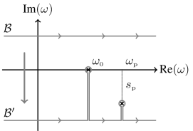
Figure 1: Illustration of the computation of the inverse Laplace Transform from equation (71). The integrand from equation (71) admits two different types of poles: either on the real axis in ${\omega=\omega_{0}={\mathbf{k}^{\prime}}\cdot\bm{\Omega}({\mathbf{J}^{\prime}})}$, or in the lower half complex plane in ${\omega=\omega_{\mathrm{p}}+\mathrm{i}s_{\mathrm{p}}}$, with ${s_{\mathrm{p}}\leq 0}$. By distorting the contour $\mathcal{B}$ into the contour $\mathcal{B}^{\prime}$ with large negative complex values, only the contributions from the residues of the poles remain. As ${s_{\mathrm{p}}\leq 0}$, for $t$ large enough, the contributions from the poles in ${\omega=\omega_{\mathrm{p}}+\mathrm{i}s_{\mathrm{p}}}$ vanish, and only the pole on the real axis contributes.

Assuming that the bath is linearly stable, ${\psi^{\mathrm{d}}_{\mathbf{k}{\mathbf{k}^{\prime}}}(\mathbf{J},{\mathbf{J}^{\prime}},\omega)}$ has poles only in the lower half of the complex $\omega$ plane (see Section 5.3.2. in Binney & Tremaine, 2008). These poles are of the generic form ${\omega=\omega_{\rm p}+\mathrm{i}s_{\rm p}}$ with ${s_{\mathrm{p}}\leq 0}$ (see the response matrix from equation (139)). Only one pole of the integrand from equation (71) is on the real axis, namely in ${\omega={\mathbf{k}^{\prime}}\cdot\bm{\Omega}({\mathbf{J}^{\prime}})}$, while all the other poles are below the real axis. Following Figure 1, the contour $\mathcal{B}$ can be distorted into the contour $\mathcal{B}^{\prime}$, so that there remains only contributions from the residues. Paying careful attention to the direction of integration, each pole contributes a ${-2\pi\mathrm{i}\text{Res}[\ldots]}$, and equation (71) becomes

$$\eta_{\mathbf{k}}(\mathbf{J},t)={(2\pi)}^{d}\sum_{{\mathbf{k}^{\prime}}}\!\!\int\!\!\mathrm{d}{\mathbf{J}^{\prime}}\,\delta F_{{\mathbf{k}^{\prime}}}({\mathbf{J}^{\prime}},0)\bigg{[}\mathrm{e}^{-\mathrm{i}{\mathbf{k}^{\prime}}\cdot\bm{\Omega}({\mathbf{J}^{\prime}})t}\,\psi^{\mathrm{d}}_{\mathbf{k}{\mathbf{k}^{\prime}}}(\mathbf{J},{\mathbf{J}^{\prime}},{\mathbf{k}^{\prime}}\!\cdot\!\bm{\Omega}({\mathbf{J}^{\prime}}))+\sum_{\mathrm{p}}\mathrm{e}^{s_{\mathrm{p}}t}\,\mathrm{e}^{-\mathrm{i}\omega_{\mathrm{p}}t}\times(\ldots)\bigg{]},$$ (72)

where the sum over “$\mathrm{p}$” runs over all the poles of ${\psi_{\mathbf{k}{\mathbf{k}^{\prime}}}^{\mathrm{d}}(\mathbf{J},{\mathbf{J}^{\prime}},\omega)}$. Since ${s_{\mathrm{p}}\leq 0}$, these modes are damped, and their contributions vanish for ${t\gg 1/|s_{\mathrm{p}}|}$. This implies, that a self-interacting bath, initially uncorrelated, will develop correlations that will settle to a steady state on timescale ${t\gg 1/|s_{\mathrm{p}}|}$, which can be assumed to be of the order of the dynamical timescale ${\sim 1/\Omega}$. Once these damped contributions have faded, equation (72) becomes

$$\eta_{\mathbf{k}}(\mathbf{J},t)={(2\pi)}^{d}\sum_{{\mathbf{k}^{\prime}}}\!\!\int\!\!\mathrm{d}{\mathbf{J}^{\prime}}\,\psi_{\mathbf{k}{\mathbf{k}^{\prime}}}^{\mathrm{d}}(\mathbf{J},{\mathbf{J}^{\prime}},{\mathbf{k}^{\prime}}\!\cdot\!\bm{\Omega}({\mathbf{J}^{\prime}}))\,\mathrm{e}^{-\mathrm{i}{\mathbf{k}^{\prime}}\cdot\bm{\Omega}({\mathbf{J}^{\prime}})t}\,\delta F_{{\mathbf{k}^{\prime}}}({\mathbf{J}^{\prime}},0).$$ (73)

Equation (73) is the direct equivalent of equation (59), when collective effects are accounted for. In this context, considering the self-gravitating amplification amounts to replacing the bare susceptibility coefficients ${\psi_{\mathbf{k}{\mathbf{k}^{\prime}}}(\mathbf{J},{\mathbf{J}^{\prime}})}$ from equation (7) by their dressed analogs ${\psi_{\mathbf{k}{\mathbf{k}^{\prime}}}^{\mathrm{d}}(\mathbf{J},{\mathbf{J}^{\prime}},\mathbf{k}\cdot\bm{\Omega}(\mathbf{J}))}$ defined by the implicit relation from equation (70). Because of the strong analogies between equations (59) and (73), when self-gravity is accounted for, the statistics of the fluctuations in the bath remain formally the same, except for a change in the pairwise interaction potential which becomes dressed, i.e. one makes the change ${\psi_{\mathbf{k}{\mathbf{k}^{\prime}}}(\mathbf{J},{\mathbf{J}^{\prime}})\to\psi_{\mathbf{k}{\mathbf{k}^{\prime}}}^{\mathrm{d}}(\mathbf{J},{\mathbf{J}^{\prime}},\mathbf{k}\cdot\bm{\Omega}(\mathbf{J}))}$. In that sense, equation (73) could be interpreted as describing the potential fluctuations present in a system where the bath particles follow the mean field orbit, i.e. ${\bm{\theta}(t)=\bm{\theta}_{0}+\bm{\Omega}(\mathbf{J})}$ and ${\mathbf{J}(t)=\mathbf{J}(0)}$, but interact via a different pairwise interaction potential dictated by the dressed susceptibility coefficients ${\psi_{\mathbf{k}{\mathbf{k}^{\prime}}}^{\mathrm{d}}(\mathbf{J},{\mathbf{J}^{\prime}},\mathbf{k}\cdot\bm{\Omega}(\mathbf{J}))}$. Starting from the fluctuations from equation (73), the correlation of the potential fluctuations in the presence of collective effects becomes

$$C_{\mathbf{k}\mathbf{k}}(\mathbf{J},{\mathbf{J}^{\prime}},t-{t^{\prime}})={} \left\langle\eta_{\mathbf{k}}(\mathbf{J},t)\,\eta_{\mathbf{k}}^{*}(\mathbf{J},{t^{\prime}})\right\rangle$$

$$={} m_{\mathrm{b}}\,{(2\pi)}^{d}\sum_{{\mathbf{k}^{\prime}}}\!\!\int\!\!\mathrm{d}{\mathbf{J}^{\prime}}\,{|\psi_{\mathbf{k}{\mathbf{k}^{\prime}}}^{\mathrm{d}}(\mathbf{J},{\mathbf{J}^{\prime}},{\mathbf{k}^{\prime}}\!\cdot\!\bm{\Omega}({\mathbf{J}^{\prime}}))|}^{2}\,F_{\mathrm{b}}({\mathbf{J}^{\prime}})\,\mathrm{e}^{-\mathrm{i}{\mathbf{k}^{\prime}}\cdot\bm{\Omega}({\mathbf{J}^{\prime}})(t-{t^{\prime}})}.$$ (74)

Following equation (48), one can immediately obtain the diffusion coefficients of a test particle undergoing such stochastic perturbations. They read

$$D_{ij}(\mathbf{J})=m_{\mathrm{b}}\,{(2\pi)}^{d+1}\sum_{\mathbf{k},{\mathbf{k}^{\prime}}}k_{i}k_{j}\!\!\int\!\!\mathrm{d}{\mathbf{J}^{\prime}}\,\delta_{\mathrm{D}}(\mathbf{k}\!\cdot\!\bm{\Omega}(\mathbf{J})-{\mathbf{k}^{\prime}}\!\cdot\!\bm{\Omega}({\mathbf{J}^{\prime}}))\,{|\psi_{\mathbf{k}{\mathbf{k}^{\prime}}}^{\mathrm{d}}(\mathbf{J},{\mathbf{J}^{\prime}})|}^{2}\,F_{\mathrm{b}}({\mathbf{J}^{\prime}}).$$ (75)

In equation (75), we recover the diffusion coefficients of the inhomogeneous BL equation, derived recently in Heyvaerts (2010); Chavanis (2012b). Let us emphasize in particular the striking similarities between the dressed diffusion coefficients from equation (75) and the bare ones obtained in equation (62). The diffusion coefficients from equation (75) describe the slow diffusion of a test particle embedded in an external bath made of $N$ particles when collective effects are accounted for, i.e. when the bath particles see the mean field potential as well as the fluctuations they themselves generate (see equation (63)). In the previous section, we discussed the physical content of the bare diffusion coefficients of the inhomogeneous Landau equation. Because of the fundamental similarities between equations (62) and (75), this discussion directly translates to the dressed diffusion coefficients of the inhomogeneous BL equation. The only difference comes from the change in the strength of the resonant couplings, which is now controlled by the squared dressed susceptibility coefficients ${{|\psi_{\mathbf{k}{\mathbf{k}^{\prime}}}^{\mathrm{d}}(\mathbf{J},{\mathbf{J}^{\prime}},\mathbf{k}\cdot\bm{\Omega}(\mathbf{J}))|}^{2}}$. Let us note that in cold dynamical systems, i.e. systems able to strongly amplify perturbations, dressing up the interactions might have a significant impact on the long-term dynamics in the system, and could even lead to instability. This was for example recently shown in Fouvry et al. (2015c) in the context of razor-thin stellar disks. Collective effects, manifested in stellar disks by strong swing amplification (Toomre, 1981), can significantly hasten the diffusion compared to the bare diffusion, leading in particular to the formation of narrow resonant ridge features in action space. In previous applications of the BL formalism (see e.g., Fouvry et al., 2015c; Benetti & Marcos, 2017), most of the effort in the computation of the dressed diffusion coefficients was dedicated to the computation of the dressed susceptibility coefficients ${\psi_{\mathbf{k}{\mathbf{k}^{\prime}}}^{\mathrm{d}}(\mathbf{J},{\mathbf{J}^{\prime}},\omega)}$, which asked for the inversion of the self-consistency definition from equation (70) via the basis method from Appendix B. In Section 8, we illustrate how the present $\eta$-formalism allows us to determine the dressed diffusion coefficients from equation (75) in the case of the one-dimensional inhomogeneous HMF model. This is one of the main strengths of the present $\eta$-formalism. It allows for the characterization of the dressed diffusion coefficients without ever having to invert the self-consistency relation from equation (70), i.e. without ever having to compute explicitly the dressed susceptibility coefficients ${\psi_{\mathbf{k}{\mathbf{k}^{\prime}}}^{\mathrm{d}}(\mathbf{J},{\mathbf{J}^{\prime}},\omega)}$.

Let us finally note that for a bath such that ${\partial F_{\mathrm{b}}/\partial\mathbf{J}=0}$, equation (70) gives ${\psi_{\mathbf{k}{\mathbf{k}^{\prime}}}^{\mathrm{d}}(\mathbf{J},{\mathbf{J}^{\prime}},\omega)=\psi_{\mathbf{k}{\mathbf{k}^{\prime}}}(\mathbf{J},{\mathbf{J}^{\prime}})}$. In that limit, collective effects can be neglected and the Landau and BL diffusion coefficients are identical. As will be show in Section 5, in these systems, the friction force by polarization also vanishes. Such a limit is of particular importance to describe the scalar resonant relaxation of isotropic spherical quasi-Keplerian systems (Bar-Or & Alexander, 2014).

5 Dynamical Friction

In the previous sections we assumed that the test particle has no influence on the bath. In that limit, the potential fluctuations induced by the bath are independent of the motion of the test particle. This led us to obtain a diffusion equation (equation (44)) for the test particle’s PDF with no advection term, i.e. with no drift term proportional to the mass of the test particle (Binney & Lacey, 1988; Binney & Tremaine, 2008). Let us note that such a limit is correct for a bath such that ${\partial F_{\mathrm{b}}/\partial\mathbf{J}=0}$, or in the limit of a test particle of zero mass, or for a purely external bath. Yet, if the test particle can influence the bath particles, there will be an advection term associated with the perturbations of the bath along the trajectory of the test particle. This component is the so-called friction force by polarization, which captures in particular the process of dynamical friction (Chandrasekhar, 1943; Tremaine & Weinberg, 1984; Nelson & Tremaine, 1999; Binney & Tremaine, 2008). For a closed system, such a friction component is necessary because of the constraint of energy conservation, i.e. any diffusion in the system must be associated with a friction. We refer to Heyvaerts et al. (2017) and references therein for a thorough discussion of this contribution. The calculations presented in this section follow Weinberg (1989); Chavanis (2012b); Heyvaerts et al. (2017) and will therefore be presented in a concise manner.

We are interested in how the potential perturbations in the bath change because of the influence of the test particle. In the presence of collective effects, i.e. assuming that bath particles interact among themselves, and if the test particle can perturb the bath particles, the specific Hamiltonian of the bath particles is

$$H_{\mathrm{b}}(\bm{\theta},\mathbf{J},t)=H_{0}(\mathbf{J})+\delta\phi_{\mathrm{t}}(\bm{\theta},\mathbf{J},t)+\delta\phi_{\mathrm{p}}(\bm{\theta},\mathbf{J},t),$$ (76)

where here, ${\delta\phi_{\mathrm{t}}(\bm{\theta},\mathbf{J},t)}$ is the perturbation of the test particle on the bath particles and ${\delta\phi_{\mathrm{p}}(\bm{\theta},\mathbf{J},t)}$ is the polarization response from the bath, which captures the bath’s self-gravity. The latter is composed of two contributions: (i) the response of the bath to the finite-$N$ fluctuations associated with the discrete number of bath particles (i.e. the potential perturbations ${\eta(\bm{\theta},\mathbf{J},t)}$ from equation (63)), (ii) the response of the bath to the perturbation ${\delta\phi_{\mathrm{t}}}$ due to the test particle. Assuming that these potential perturbations are small compared to the mean Hamiltonian $H_{0}$, similarly to equation (4.2), the evolution of the bath is given by the linearized Klimontovich equation reading

$$0={} \mathinner{\dfrac{\partial{}\delta F}{\partial{t}}}+\big{[}\delta F,H_{0}\big{]}+\big{[}F_{\mathrm{b}},\delta\phi_{\mathrm{t}}+\delta\phi_{\mathrm{p}}\big{]}$$

$$={} \mathinner{\dfrac{\partial{}\delta F}{\partial{t}}}+\mathinner{\dfrac{\partial{}\delta F}{\partial{\bm{\theta}}}}\cdot\bm{\Omega}(\mathbf{J})-\mathinner{\dfrac{\partial{}F_{\mathrm{b}}}{\partial{\mathbf{J}}}}\cdot\mathinner{\dfrac{\partial{}[\delta\phi_{\mathrm{t}}+\delta\phi_{\mathrm{p}}]}{\partial{\bm{\theta}}}},$$ (77)

where ${\delta F}$ stands for the fluctuations in the bath’s DF.

Following equation (66), it is straightforward to write the Laplace-Fourier transform of equation (5) to obtain

$$\delta\widetilde{F}_{\mathbf{k}}(\mathbf{J},\omega)=-\frac{\delta F_{\mathbf{k}}(\mathbf{J},0)}{\mathrm{i}(\omega-\mathbf{k}\!\cdot\!\bm{\Omega}(\mathbf{J}))}-\frac{\mathbf{k}\!\cdot\!\partial F_{\mathrm{b}}/\partial\mathbf{J}}{\omega-\mathbf{k}\!\cdot\!\bm{\Omega}(\mathbf{J})}\,\delta\widetilde{\phi}_{\mathbf{k}}^{\mathrm{t}}(\mathbf{J},\omega)-\frac{\mathbf{k}\!\cdot\!\partial F_{\mathrm{b}}/\partial\mathbf{J}}{\omega-\mathbf{k}\!\cdot\!\bm{\Omega}(\mathbf{J})}\,\delta\widetilde{\phi}_{\mathbf{k}}^{\mathrm{p}}(\mathbf{J},\omega).$$ (78)

Similarly to equation (56), the bath’s polarization response ${\delta\phi_{\mathrm{p}}}$ results from the fluctuations of the bath’s DF, ${\delta F}$, so that we can write

$$\delta\widetilde{\phi}_{\mathbf{k}}^{\mathrm{p}}(\mathbf{J},\omega)={(2\pi)}^{d}\sum_{{\mathbf{k}^{\prime}}}\!\!\int\!\!\mathrm{d}{\mathbf{J}^{\prime}}\,\psi_{\mathbf{k}{\mathbf{k}^{\prime}}}(\mathbf{J},{\mathbf{J}^{\prime}})\,\delta\widetilde{F}_{{\mathbf{k}^{\prime}}}({\mathbf{J}^{\prime}},\omega).$$ (79)

Let us then act on both sides of equation (78) with the same operator as in the r.h.s. of equation (79). Similarly to equation (68), we get the self-consistency relation

$$\delta\widetilde{\phi}_{\mathbf{k}}^{\mathrm{p}}(\mathbf{J},\omega)={} -{(2\pi)}^{d}\sum_{{\mathbf{k}^{\prime}}}\!\!\int\!\!\mathrm{d}{\mathbf{J}^{\prime}}\,\frac{{\mathbf{k}^{\prime}}\!\cdot\!\partial F_{\mathrm{b}}/\partial{\mathbf{J}^{\prime}}}{\omega-{\mathbf{k}^{\prime}}\!\cdot\!\bm{\Omega}({\mathbf{J}^{\prime}})}\,\psi_{\mathbf{k}{\mathbf{k}^{\prime}}}(\mathbf{J},{\mathbf{J}^{\prime}})\,\delta\widetilde{\phi}_{{\mathbf{k}^{\prime}}}^{\mathrm{p}}({\mathbf{J}^{\prime}},\omega)$$

$$-{(2\pi)}^{d}\sum_{{\mathbf{k}^{\prime}}}\!\!\int\!\!\mathrm{d}{\mathbf{J}^{\prime}}\,\frac{\delta F_{{\mathbf{k}^{\prime}}}({\mathbf{J}^{\prime}},0)}{\mathrm{i}(\omega-{\mathbf{k}^{\prime}}\!\cdot\!\bm{\Omega}({\mathbf{J}^{\prime}}))}\,\psi_{\mathbf{k}{\mathbf{k}^{\prime}}}(\mathbf{J},{\mathbf{J}^{\prime}})$$

$$-{(2\pi)}^{d}\sum_{{\mathbf{k}^{\prime}}}\!\!\int\!\!\mathrm{d}{\mathbf{J}^{\prime}}\,\frac{{\mathbf{k}^{\prime}}\!\cdot\!\partial F_{\mathrm{b}}/\partial\mathbf{J}}{\omega-{\mathbf{k}^{\prime}}\!\cdot\!\bm{\Omega}({\mathbf{J}^{\prime}})}\,\psi_{\mathbf{k}{\mathbf{k}^{\prime}}}(\mathbf{J},{\mathbf{J}^{\prime}})\,\delta\widetilde{\phi}_{{\mathbf{k}^{\prime}}}^{\mathrm{t}}({\mathbf{J}^{\prime}},\omega),$$ (80)

which takes again the form of a Fredholm equation of the second kind for the polarization response ${\delta\widetilde{\phi}_{\mathbf{k}}^{\mathrm{p}}(\mathbf{J},\omega)}$. In the r.h.s. of that equation, the first line corresponds to the kernel of the relation and captures the strength of the self-gravitating amplification in the bath and is sourced by the gradients of the bath’s DF. This equation possesses two source terms, namely the initial finite-$N$ fluctuations in the bath (second term) and the potential perturbation from the test particle (third term). In order to ease the inversion of this equation, and simplify the discussion of its physical content, let us now rely on the basis method introduced in Appendix B.

Relying on equation (140) to express the bare susceptibility elements ${\psi_{\mathbf{k}{\mathbf{k}^{\prime}}}(\mathbf{J},{\mathbf{J}^{\prime}})}$ with the basis elements, we introduce the vectors $\widetilde{\mathbf{P}}$, $\widetilde{\mathbf{T}}$ as

$$\delta\widetilde{\phi}_{\mathbf{k}}^{\mathrm{p}}(\mathbf{J},\omega)=\sum_{\alpha}\widetilde{\mathbf{P}}_{\alpha}(\omega)\,\psi_{\mathbf{k}}^{(\alpha)}(\mathbf{J})\;\;\;;\;\;\;\delta\widetilde{\phi}_{\mathbf{k}}^{\mathrm{t}}(\mathbf{J},\omega)=\sum_{\alpha}\widetilde{\mathbf{T}}_{\alpha}(\omega)\,\psi_{\mathbf{k}}^{(\alpha)}(\mathbf{J}).$$ (81)

To decompose the fluctuating source term from equation (5), we also introduce the vector $\widetilde{\mathbf{S}}$

$$\widetilde{\mathbf{S}}_{\alpha}(\omega)={(2\pi)}^{d}\sum_{{\mathbf{k}^{\prime}}}\!\!\int\!\!\mathrm{d}{\mathbf{J}^{\prime}}\,\frac{\delta F_{{\mathbf{k}^{\prime}}}({\mathbf{J}^{\prime}},0)}{\mathrm{i}(\omega-{\mathbf{k}^{\prime}}\!\cdot\!\bm{\Omega}({\mathbf{J}^{\prime}}))}\,\psi_{{\mathbf{k}^{\prime}}}^{(\alpha)*}({\mathbf{J}^{\prime}}).$$ (82)

describing the initial finite-$N$ fluctuations in the system’s DF. The self-consistency equation (5) then takes the short form

$$\widetilde{\mathbf{P}}(\omega)=\widehat{\mathbf{M}}(\omega)\!\cdot\!\widetilde{\mathbf{P}}(\omega)+\widetilde{\mathbf{S}}(\omega)+\widehat{\mathbf{M}}(\omega)\!\cdot\!\widetilde{\mathbf{T}}(\omega),$$ (83)

where $\widehat{\mathbf{M}}$ is the bath’s response matrix introduced in equation (139). Here, ${\widetilde{\mathbf{P}}(\omega)}$ characterizes the polarization response of the bath, ${\widetilde{\mathbf{S}}(\omega)}$ the initial finite-$N$ fluctuations in the system’s DF, and ${\widetilde{\mathbf{T}}(\omega)}$ the perturbation from the test particle. This third term is the one that captures the back-reaction of the test particle on the bath and leads to the associated friction force by polarization. Assuming that the bath is linearly stable (i.e. ${\omega\to{[\mathbf{I}-\widehat{\mathbf{M}}(\omega)]}^{-1}}$ has no poles in the upper half complex plane), equation (83) is straightforward to invert for ${\widetilde{\mathbf{P}}(\omega)}$. It becomes

$$\widetilde{\mathbf{P}}(\omega)={\big{[}\mathbf{I}-\widehat{\mathbf{M}}(\omega)\big{]}}^{-1}\!\!\cdot\widetilde{\mathbf{S}}(\omega)+\big{\{}{\big{[}\mathbf{I}-\widehat{\mathbf{M}}(\omega)\big{]}}^{-1}-\mathbf{I}\big{\}}\!\cdot\!\widetilde{\mathbf{T}}(\omega),$$ (84)

which in the absence of collective effects is simply ${\widetilde{\mathbf{P}}(\omega)=\widetilde{\mathbf{S}}(\omega)+\widehat{\mathbf{M}}(\omega)\cdot\widetilde{\mathbf{T}}(\omega)}$.

Before writing down the time version of equation (84), we need first to express explicitly the source term due to the test particle, ${\widetilde{\mathbf{T}}(\omega)}$. Noting the position of the test particle at time $t$ with ${(\bm{\theta}_{\mathrm{t}}(t),\mathbf{J}_{\mathrm{t}}(t))}$, we can write ${\delta\phi_{\mathbf{k}}^{\mathrm{t}}(\mathbf{J},t)}$ as

$$\delta\phi_{\mathbf{k}}^{\mathrm{t}}(\mathbf{J},t)=m_{\mathrm{t}}\sum_{{\mathbf{k}^{\prime}}}\psi_{\mathbf{k}{\mathbf{k}^{\prime}}}(\mathbf{J},\mathbf{J}_{\mathrm{t}}(t))\,\mathrm{e}^{-\mathrm{i}{\mathbf{k}^{\prime}}\cdot\bm{\theta}_{\mathrm{t}}(t)},$$ (85)

where $m_{\mathrm{t}}$ is the mass of the test particle. Relying on the timescale separation between the fast timescale of the mean field orbital motion and the slow timescale of diffusion, let us then replace in equation (85) the motion of the test particle by its mean field motion, so that ${\bm{\theta}_{\mathrm{t}}(t)=\bm{\theta}_{\mathrm{t}}^{0}+\bm{\Omega}(\mathbf{J}_{\mathrm{t}})}$ and ${\mathbf{J}_{\mathrm{t}}(t)=\mathbf{J}_{\mathrm{t}}}$, where $\bm{\theta}_{\mathrm{t}}^{0}$ is the initial phase of the test particle. Following equation (81), the coefficients ${\widetilde{\mathbf{T}}_{\alpha}(\omega)}$ are then straightforward to write, and one gets

$$\widetilde{\mathbf{T}}_{\alpha}(\omega)=m_{\mathrm{t}}\sum_{{\mathbf{k}^{\prime}}}\frac{\mathrm{e}^{-\mathrm{i}{\mathbf{k}^{\prime}}\cdot\bm{\theta}_{\mathrm{t}}^{0}}}{\mathrm{i}(\omega-{\mathbf{k}^{\prime}}\!\cdot\!\bm{\Omega}(\mathbf{J}_{\mathrm{t}}))}\,\psi_{{\mathbf{k}^{\prime}}}^{(\alpha)*}(\mathbf{J}_{\mathrm{t}}).$$ (86)

Having specified all the terms appearing in equation (84), we may then take the inverse Laplace transform of this equation. This calculation is essentially identical to the one performed in equation (72). In equation (84), there exist two kinds of poles: (i) poles on the real axis coming from the source terms ${\widetilde{\mathbf{S}}(\omega)}$ and ${\widetilde{\mathbf{T}}(\omega)}$, (ii) poles below the real axis coming from the susceptibility matrix ${{[\mathbf{I}-\widehat{\mathbf{M}}(\omega)]}^{-1}}$. We then consider times long enough for the contributions from the damped modes to vanish. After a straightforward calculation, we obtain from equation (84) that

$$\delta\phi_{\mathbf{k}}^{\mathrm{p}}(\mathbf{J},t)={} {(2\pi)}^{d}\sum_{{\mathbf{k}^{\prime}}}\!\!\int\!\!\mathrm{d}{\mathbf{J}^{\prime}}\,\psi_{\mathbf{k}{\mathbf{k}^{\prime}}}^{\mathrm{d}}(\mathbf{J},{\mathbf{J}^{\prime}},{\mathbf{k}^{\prime}}\!\cdot\!\bm{\Omega}({\mathbf{J}^{\prime}}))\,\mathrm{e}^{-\mathrm{i}{\mathbf{k}^{\prime}}\cdot\bm{\Omega}({\mathbf{J}^{\prime}})t}\,\delta F_{{\mathbf{k}^{\prime}}}({\mathbf{J}^{\prime}},0)$$

$$+m_{\mathrm{t}}\sum_{{\mathbf{k}^{\prime}}}\big{\{}\psi_{\mathbf{k}{\mathbf{k}^{\prime}}}^{\mathrm{d}}(\mathbf{J},\mathbf{J}_{\mathrm{t}},{\mathbf{k}^{\prime}}\!\cdot\!\bm{\Omega}(\mathbf{J}_{\mathrm{t}}))-\psi_{\mathbf{k}{\mathbf{k}^{\prime}}}(\mathbf{J},\mathbf{J}_{\mathrm{t}})\big{\}}\,\mathrm{e}^{-\mathrm{i}{\mathbf{k}^{\prime}}\cdot\bm{\theta}_{\mathrm{t}}(t)}$$

$$={} \eta_{\mathbf{k}}(\mathbf{J},t)+h_{\mathbf{k}}^{\rm fric}(\mathbf{J},t),$$ (87)

where we used equation (138) to express the dressed susceptibility coefficients without resorting to the basis elements. In equation (5), we introduced the two components of the polarization response of the bath. Here, ${\eta_{\mathbf{k}}(\mathbf{J},t)}$ was already obtained in equation (73) and stands for the dressed potential fluctuations present in the system as a result of the finite-$N$ fluctuations from the bath (i.e. it is sourced by ${\delta F_{{\mathbf{k}^{\prime}}}({\mathbf{J}^{\prime}},0)}$). The second contribution, ${h_{\mathbf{k}}^{\rm fric}(\mathbf{J},t)}$, captures the friction force by polarization, and describes the dressed potential perturbations present in the bath as a result of the presence of the test particle. Let us note that these two potential perturbations have some fundamental differences. On the one hand, ${\eta_{\mathbf{k}}(\mathbf{J},t)}$ is truly a stochastic perturbation. It is of zero mean, depends on the bath’s realization, and its amplitude is proportional to $\sqrt{m_{\mathrm{b}}}$. On the other hand, because it only depends on the mean field parameters of the bath, ${h_{\mathbf{k}}^{\rm fric}(\mathbf{J},t)}$ should be seen as a non-stochastic perturbation. It is of non-zero mean, and its amplitude is proportional to $m_{\mathrm{t}}$. The more massive the test particle, the stronger the friction force. In Section 4.2, we have already shown how the correlation of ${\eta_{\mathbf{k}}(\mathbf{J},t)}$ leads to the diffusion coefficient of the inhomogeneous BL equation. Let us now focus on the contribution of ${h_{\mathbf{k}}^{\rm fric}(\mathbf{J},t)}$ to the diffusion equation for the test particle. The associated contribution in equation (16) takes the form

$$\mathrm{i}\sum_{\mathbf{k}}\mathbf{k}\left\langle h_{\mathbf{k}}^{\rm fric}(\mathbf{J},t)\,\mathrm{e}^{\mathrm{i}\mathbf{k}\cdot\bm{\theta}(t)}\,\varphi(\mathbf{J},t)\right\rangle={} \mathrm{i}m_{\mathrm{t}}\sum_{\mathbf{k},{\mathbf{k}^{\prime}}}\mathbf{k}\left\langle\big{\{}\psi_{\mathbf{k}{\mathbf{k}^{\prime}}}^{\mathrm{d}}(\mathbf{J},\mathbf{J},{\mathbf{k}^{\prime}}\!\cdot\!\bm{\Omega}(\mathbf{J}))-\psi_{\mathbf{k}{\mathbf{k}^{\prime}}}(\mathbf{J},\mathbf{J})\big{\}}\,\mathrm{e}^{\mathrm{i}(\mathbf{k}-{\mathbf{k}^{\prime}})\cdot\bm{\theta}(t)}\,\varphi(\mathbf{J},t)\right\rangle$$

$$={} -\mathbf{F}_{\rm pol}(\mathbf{J},t)\,P(\mathbf{J},t).$$ (88)

To obtain the second line of equation (86), we followed the same assumption as in equation (86), and assumed that the motion of the test particle is given by ${\bm{\theta}(t)=\bm{\theta}_{0}+\bm{\Omega}(\mathbf{J})t}$ and ${\mathbf{J}(t)=\mathbf{J}}$. The ensemble average from equation (5) then only amounts to averaging over the initial phase $\bm{\theta}_{0}$ of the test particle: it is straightforward and imposes ${\mathbf{k}={\mathbf{k}^{\prime}}}$. Finally, we also used the definition of the test particle’s PDF, ${P(\mathbf{J},t)=\langle\varphi(\mathbf{J},t)\rangle}$, and introduced the friction force by polarization ${\mathbf{F}_{\rm pol}(\mathbf{J},t)}$ defined as

$$\mathbf{F}_{\rm pol}(\mathbf{J},t)={} -\mathrm{i}m_{\mathrm{t}}\sum_{\mathbf{k}}\mathbf{k}\,\big{\{}\psi_{\mathbf{k}\mathbf{k}}^{\mathrm{d}}(\mathbf{J},\mathbf{J},\mathbf{k}\!\cdot\!\bm{\Omega}(\mathbf{J}))-\psi_{\mathbf{k}\mathbf{k}}(\mathbf{J},\mathbf{J})\big{\}}$$

$$={} m_{\mathrm{t}}\sum_{\mathbf{k}}\mathbf{k}\,\text{Im}\big{[}\psi_{\mathbf{k}\mathbf{k}}^{\mathrm{d}}(\mathbf{J},\mathbf{J},\mathbf{k}\!\cdot\!\bm{\Omega}(\mathbf{J}))\big{]},$$ (89)

where we used the fact that ${\psi_{\mathbf{k}\mathbf{k}}(\mathbf{J},\mathbf{J})}$ and ${\mathbf{F}_{\rm pol}(\mathbf{J},t)}$ are real. In Equation (5), we recover a result already obtained in equation (53) of Weinberg (1989). We do not pursue further the calculation of ${\mathbf{F}_{\rm pol}(\mathbf{J},t)}$ and refer to equation (54) of Chavanis (2012b) to obtain an integral expression for ${\text{Im}[\psi_{\mathbf{k}\mathbf{k}}^{\mathrm{d}}(\mathbf{J},\mathbf{J},\mathbf{k}\cdot\bm{\Omega}(\mathbf{J}))]}$. The friction force by polarization finally becomes

$$\mathbf{F}_{\rm pol}(\mathbf{J},t)=m_{\mathrm{t}}\pi{(2\pi)}^{d}\sum_{\mathbf{k},{\mathbf{k}^{\prime}}}\mathbf{k}\!\!\int\!\!\mathrm{d}{\mathbf{J}^{\prime}}\,\delta_{\mathrm{D}}(\mathbf{k}\!\cdot\!\bm{\Omega}(\mathbf{J})-{\mathbf{k}^{\prime}}\!\cdot\!\bm{\Omega}({\mathbf{J}^{\prime}}))\,{|\psi_{\mathbf{k}{\mathbf{k}^{\prime}}}^{\mathrm{d}}(\mathbf{J},{\mathbf{J}^{\prime}},\mathbf{k}\!\cdot\!\bm{\Omega}(\mathbf{J}))|}^{2}\,\bigg{(}{\mathbf{k}^{\prime}}\!\cdot\!\mathinner{\dfrac{\partial{}F_{\mathrm{b}}({\mathbf{J}^{\prime}},t)}{\partial{{\mathbf{J}^{\prime}}}}}\bigg{)}.$$ (90)

Deriving in equation (90) the expression of the dressed friction force by polarization is the main result of this section. Here, we recovered the expression of the bare resonant dynamical friction in particular obtained in equation (30) of Lynden-Bell & Kalnajs (1972), and equation (65) of Tremaine & Weinberg (1984), as well as its dressed generalisation obtained among others in equation (53) of Weinberg (1989), equation (24) of Seguin & Dupraz (1994), or in equation (113) of Chavanis (2012b).

6 The Balescu-Lenard equation

In the previous sections, we derived successively the two components involved in the long-term evolution of a massive test particle embedded in a self-gravitating discrete bath. First, in equation (75), we derived the diffusion coefficients, ${D_{ij}(\mathbf{J})}$, sourced by the temporal correlations of the finite-$N$ dressed perturbations present in the bath. Second, in equation (16), we derived the friction force by polarization, ${F_{\rm pol}(\mathbf{J})}$, which captures the dressed back-reaction of the perturbations in the bath induced by the massive test particle. Gathering these two components, the diffusion equation (16) takes the form

$$\mathinner{\dfrac{\partial{}P(\mathbf{J},t)}{\partial{t}}}={} \mathinner{\dfrac{\partial{}}{\partial{\mathbf{J}}}}\!\cdot\!\bigg{[}-\mathbf{F}_{\rm pol}(\mathbf{J},t)\,P(\mathbf{J},t)+\frac{1}{2}\mathbf{D}(\mathbf{J},t)\!\cdot\!\mathinner{\dfrac{\partial{}P(\mathbf{J},t)}{\partial{\mathbf{J}}}}\bigg{]}$$

$$={} \pi{(2\pi)}^{d}\mathinner{\dfrac{\partial{}}{\partial{\mathbf{J}}}}\!\cdot\!\bigg{[}\sum_{\mathbf{k},{\mathbf{k}^{\prime}}}\!\int\!\!\mathrm{d}{\mathbf{J}^{\prime}}\,\delta_{\mathrm{D}}(\mathbf{k}\!\cdot\!\bm{\Omega}(\mathbf{J})-{\mathbf{k}^{\prime}}\!\cdot\!\bm{\Omega}({\mathbf{J}^{\prime}}))\,{|\psi_{\mathbf{k}{\mathbf{k}^{\prime}}}^{\mathrm{d}}(\mathbf{J},{\mathbf{J}^{\prime}},\mathbf{k}\!\cdot\!\bm{\Omega}(\mathbf{J}))|}^{2}$$

$$\times\bigg{(}m_{\mathrm{b}}\,\mathbf{k}\!\cdot\!\mathinner{\dfrac{\partial{}}{\partial{\mathbf{J}}}}-m_{\mathrm{t}}\,{\mathbf{k}^{\prime}}\!\cdot\!\mathinner{\dfrac{\partial{}}{\partial{{\mathbf{J}^{\prime}}}}}\bigg{)}\,P(\mathbf{J},t)\,F_{\mathrm{b}}({\mathbf{J}^{\prime}},t)\bigg{]}.$$ (91)

In equation (6), we recover exactly the inhomogeneous BL equation, already obtained in equation (38) of Heyvaerts (2010) and equation (56) of Chavanis (2012b). This equation describes the evolution of a given test particle embedded in a discrete system of $N$ particles. As emphasized previously, in the limit where collective effects are not accounted for, the BL equation (6) becomes the inhomogeneous Landau equation. Such a limit is obtained by replacing in equation (6) the dressed susceptibility coefficients ${\psi_{\mathbf{k}{\mathbf{k}^{\prime}}}^{\mathrm{d}}(\mathbf{J},{\mathbf{J}^{\prime}},\omega)}$ by their bare analogs ${\psi_{\mathbf{k}{\mathbf{k}^{\prime}}}(\mathbf{J},{\mathbf{J}^{\prime}})}$ introduced in equation (7). In particular, for a bath such that ${\partial F_{\mathrm{b}}/\partial\mathbf{J}=0}$, these two equations are equivalent.

The BL equation (6) is composed of two components. First, a diffusion component associated with the term proportional to ${m_{\mathrm{b}}\mathbf{k}\cdot\partial/\partial\mathbf{J}}$. This diffusion component is sourced by the correlations in the bath potential fluctuations. It is proportional to the mass of the bath particles ${m_{\mathrm{b}}=M/N}$, and vanishes in the limit of a collisionless bath, i.e. in the limit ${N\to+\infty}$. The second component of equation (6) is the friction component and is proportional to ${m_{\mathrm{t}}\,{\mathbf{k}^{\prime}}\cdot\partial/\partial{\mathbf{J}^{\prime}}}$. This friction component is sourced by the back-reaction of the test particle on the bath. It is therefore proportional to the mass $m_{\mathrm{t}}$ of the test particle, and is responsible for mass segregation. It does not vanish in the limit of a collisionless bath, i.e. in the limit ${N\to+\infty}$. This friction component also vanishes in the limit of a bath satisfying ${\partial F_{\mathrm{b}}/\partial\mathbf{J}=0}$.

Equation (6) describes the evolution of the statistics of a test particle (described via the PDF ${P(\mathbf{J},t)}$), when embedded in a bath (described by the DF ${F_{\mathrm{b}}(\mathbf{J},t)}$). It is then straightforward to use equation (6) to obtain the self-consistent evolution equation satisfied by the bath’s DF when diffusing on long-term timescales. This only amounts to assuming that the statistics of the test particle is given by the statistics of the bath particles, i.e. one performs the replacement ${P(\mathbf{J},t)\to F_{\mathrm{b}}(\mathbf{J},t)}$. Such a replacement transforms the differential equation (6) into a self-consistent integro-differential equation for the bath’s DF. This is the self-consistent inhomogeneous BL equation (Heyvaerts, 2010; Chavanis, 2012b), reading

$$\mathinner{\dfrac{\partial{}F_{\mathrm{b}}(\mathbf{J},t)}{\partial{t}}}={} \pi{(2\pi)}^{d}\mathinner{\dfrac{\partial{}}{\partial{\mathbf{J}}}}\!\cdot\!\bigg{[}\sum_{\mathbf{k},{\mathbf{k}^{\prime}}}\!\int\!\!\mathrm{d}{\mathbf{J}^{\prime}}\,\delta_{\mathrm{D}}(\mathbf{k}\!\cdot\!\bm{\Omega}(\mathbf{J})-{\mathbf{k}^{\prime}}\!\cdot\!\bm{\Omega}({\mathbf{J}^{\prime}}))\,{|\psi_{\mathbf{k}{\mathbf{k}^{\prime}}}^{\mathrm{d}}(\mathbf{J},{\mathbf{J}^{\prime}},\mathbf{k}\!\cdot\!\bm{\Omega}(\mathbf{J}))|}^{2}$$

$$\times\bigg{(}m_{\mathrm{b}}\,\mathbf{k}\!\cdot\!\mathinner{\dfrac{\partial{}}{\partial{\mathbf{J}}}}-m_{\mathrm{b}}\,{\mathbf{k}^{\prime}}\!\cdot\!\mathinner{\dfrac{\partial{}}{\partial{{\mathbf{J}^{\prime}}}}}\bigg{)}\,F_{\mathrm{b}}(\mathbf{J},t)\,F_{\mathrm{b}}({\mathbf{J}^{\prime}},t)\bigg{]}.$$ (92)

As emphasized in Heyvaerts et al. (2017), let us finally recall that the self-consistent BL equation (6) satisfies a $H$-theorem for Boltzmann’s entropy. As a result, the BL equation admits the Boltzmann’s DF ${F_{\mathrm{b}}(\mathbf{J})\propto\mathrm{e}^{-\beta H_{0}(\mathbf{J})}}$ as an equilibrium solution. Moreover, for such a thermal DF, it is straightforward to show that the diffusion tensor, ${D_{ij}(\mathbf{J})}$, from equation (75) and the friction force by polarization, ${F_{\rm pol}(\mathbf{J})}$, from equation (90) satisfy a generalized fluctuation-dissipation relation of the form

$${\big{[}\mathbf{F}_{\rm pol}(\mathbf{J})\big{]}}_{i}=-\frac{1}{2}\beta\,\Omega_{j}(\mathbf{J})\,D_{ij}(\mathbf{J}),$$ (93)

where the sum over $j$ is implied. This equation was already put forward in equation (3.12) of Binney & Lacey (1988), and equation (119) of Chavanis (2012b).

It is also straightforward to generalize equation (6) to a multi-mass bath. Indeed, let us assume that the bath is composed of multiple components of individual mass $m_{\alpha}$, $m_{\beta}$, etc. Each component is described by a quasi-stationary DF of the form ${F_{\alpha}(\mathbf{J},t)}$, following the convention ${\!\int\!\mathrm{d}\bm{\theta}\mathrm{d}\mathbf{J}\,F_{\alpha}=M_{\alpha}}$, where $M_{\alpha}$ is the total mass of the component $\alpha$. Equation (6) can then be generalized to describe the self-consistent long-term evolution of the component $\alpha$, under the effects of the stochastic perturbations from itself and all other components. It reads

$$\mathinner{\dfrac{\partial{}F_{\alpha}(\mathbf{J},t)}{\partial{t}}}={} \pi{(2\pi)}^{d}\mathinner{\dfrac{\partial{}}{\partial{\mathbf{J}}}}\!\cdot\!\bigg{[}\sum_{\mathbf{k},{\mathbf{k}^{\prime}}}\!\int\!\!\mathrm{d}{\mathbf{J}^{\prime}}\,\delta_{\mathrm{D}}(\mathbf{k}\!\cdot\!\bm{\Omega}(\mathbf{J})-{\mathbf{k}^{\prime}}\!\cdot\!\bm{\Omega}({\mathbf{J}^{\prime}}))\,{|\psi_{\mathbf{k}{\mathbf{k}^{\prime}}}^{\mathrm{d}}(\mathbf{J},{\mathbf{J}^{\prime}},\mathbf{k}\!\cdot\!\bm{\Omega}(\mathbf{J}))|}^{2}$$

$$\times\sum_{\beta}\bigg{(}m_{\beta}\,\mathbf{k}\!\cdot\!\mathinner{\dfrac{\partial{}}{\partial{\mathbf{J}}}}-m_{\alpha}\,{\mathbf{k}^{\prime}}\!\cdot\!\mathinner{\dfrac{\partial{}}{\partial{{\mathbf{J}^{\prime}}}}}\bigg{)}\,F_{\alpha}(\mathbf{J},t)\,F_{\beta}({\mathbf{J}^{\prime}},t)\bigg{]}.$$ (94)

where the sum on “$\beta$” runs over all components. In the multi-component case, the dressed susceptibility coefficients ${\psi_{\mathbf{k}{\mathbf{k}^{\prime}}}^{\mathrm{d}}(\mathbf{J},{\mathbf{J}^{\prime}},\omega)}$ involve now all the active components in the self-gravitating amplification. As a consequence, the self-consistency definition from equation (70) becomes here

$$\psi_{\mathbf{k}{\mathbf{k}^{\prime}}}^{\mathrm{d}}(\mathbf{J},{\mathbf{J}^{\prime}},\omega)=-{(2\pi)}^{d}\sum_{{\mathbf{k}^{\prime\prime}}}\!\!\int\!\!\mathrm{d}{\mathbf{J}^{\prime\prime}}\,\frac{{\mathbf{k}^{\prime\prime}}\!\cdot\!\partial(\sum_{\beta}F_{\beta}({\mathbf{J}^{\prime\prime}}))/\partial{\mathbf{J}^{\prime\prime}}}{\omega-{\mathbf{k}^{\prime\prime}}\!\cdot\!\bm{\Omega}({\mathbf{J}^{\prime\prime}})}\,\psi_{\mathbf{k}{\mathbf{k}^{\prime\prime}}}(\mathbf{J},{\mathbf{J}^{\prime\prime}})\,\psi_{{\mathbf{k}^{\prime\prime}}{\mathbf{k}^{\prime}}}^{\mathrm{d}}({\mathbf{J}^{\prime\prime}},{\mathbf{J}^{\prime}},\omega)+\psi_{\mathbf{k}{\mathbf{k}^{\prime}}}(\mathbf{J},{\mathbf{J}^{\prime}}).$$ (95)

Let us note that the multi-mass equation (6) allows for mass segregation between the different components, because the friction force is proportional to the mass of the considered component. We refer to Heyvaerts et al. (2017) and references therein for a detailed discussion of the physical content of the inhomogeneous BL equation.

As a final remark, as pointed out in Weinberg (1993); Heyvaerts (2010); Chavanis (2013), one can assume local homogeneity in the inhomogeneous BL equation (6), to recover a diffusion equation in velocity space, the so-called homogeneous Balescu-Lenard equation, as given for example in equation (47) in Heyvaerts (2010), and equation (E.1) in Chavanis (2013). In the limit where collective effects are not accounted for, this equation reduces to the homogeneous Landau equation (see for example equation (39) in Chavanis (2013)). This diffusion equation comes at the price of truncating the interactions on both large scales (to account for the finite size of the system), and small scales (to account for strong collisions), leading to the appearance of the Coulomb logarithm. As shown in Chavanis (2013), the homogeneous Landau equation is equivalent to the classical Fokker-Planck diffusion coefficients sourced by weak encounters, as given by the Rosenbluth potentials in equation (7.83a) in Binney & Tremaine (2008). We do not pursue here the discussion of the homogeneous limit, and refer to Chavanis (2013) for a detailed investigation of the equivalences of these various approaches.

7 Dressed diffusion by external perturbations

In the previous sections, we investigated the long-term evolution of a test particle subject to (bare or dressed) stochastic potential perturbations from an external bath constituted of a finite number of particles. This allowed us to recover in equations (62) and (75) the diffusion coefficients of the inhomogeneous Landau and BL equations, and in equation (6) the full self-consistent kinetic equation. The associated diffusion coefficients are often said to capture an internally induced long-term evolution, in the sense that finite-$N$ fluctuations can be seen as self-generated perturbations. Yet, as already emphasized in the Introduction, collisionless systems (i.e. in the limit ${N\to\infty}$) can also undergo a long-term diffusion as a result of external potential fluctuations. Such diffusion was first characterized in Binney & Lacey (1988), and generalized in Weinberg (2001a) to account for collective effects. See also e.g., Pichon & Aubert (2006); Chavanis (2012a); Nardini et al. (2012); Fouvry et al. (2015a) for a revisit of this equation. Let us now show how the present $\eta$-formalism and the result from equation (48) allow for a straightforward recovery of these diffusion coefficients.

We are interested in describing the long-term evolution of a collisionless self-gravitating quasi-stationary system undergoing some external stochastic perturbations ${\delta\phi_{\rm ext}(\mathbf{x},t)}$. Assuming the mean field system to be integrable, we may then expand the DF and the specific Hamiltonian of this collisionless system as

$$F_{\rm sys}(\bm{\theta},\mathbf{J},t)=F(\mathbf{J},t)+\delta F(\bm{\theta},\mathbf{J},t),$$ (96)

and

$$H_{\rm sys}(\bm{\theta},\mathbf{J},t)={} H_{0}(\mathbf{J})+\delta\phi_{\rm ext}(\bm{\theta},\mathbf{J},t)+\delta\phi_{\mathrm{p}}(\bm{\theta},\mathbf{J},t)$$

$$={} H_{0}(\mathbf{J})+\eta(\bm{\theta},\mathbf{J},t),$$ (97)

where ${H_{0}(\mathbf{J})}$ is the mean field Hamiltonian of the system associated with the mean field quasi-stationary DF of the system ${F(\mathbf{J},t)}$. This Hamiltonian defines the orbital frequencies ${\bm{\Omega}(\mathbf{J})=\partial H_{0}/\partial\mathbf{J}}$, driving the unperturbed motions in the system. We also introduced two potential perturbations. Here, ${\delta\phi_{\rm ext}(\bm{\theta},\mathbf{J},t)}$ is the stochastic external perturbation felt by the system. In order to rely on Novikov’s theorem (equation (17)), we assume that these perturbations are small (i.e. ${\delta\phi_{\rm ext}\ll H_{0}}$), of zero mean, Gaussian, and stationary in time. Equation (7) also involves ${\delta\phi_{\mathrm{p}}(\bm{\theta},\mathbf{J},t)}$, the polarization response of the self-gravitating system to the presence of the external perturbations. In particular, the polarization perturbation satisfies the self-consistency requirement ${\delta\phi_{\mathrm{p}}(\mathbf{x},t)=\!\int\!\mathrm{d}{\mathbf{x}^{\prime}}\mathrm{d}{\mathbf{v}^{\prime}}\psi(\mathbf{x},\mathbf{x}^{\prime})\,\delta F({\mathbf{x}^{\prime}},{\mathbf{v}^{\prime}},t)}$. Following equation (8), the sum of the two potential perturbations ${\eta=\delta\phi_{\rm ext}+\delta\phi_{\mathrm{p}}}$ corresponds to the full stochastic potential perturbations felt by the collisionless system of interest. As given by the $\eta$-formalism, these fluctuations will drive a long-term distortion of the system’s orbital structure. In order to evaluate the associated diffusion coefficients from equation (48), one must therefore characterize the properties of ${\eta(\bm{\theta},\mathbf{J},t)}$. The differences of the present calculations with the previous calculations of the Landau and BL diffusion coefficients are twofold. First, here the external perturbations ${\delta\phi_{\rm ext}(\mathbf{x},t)}$ can be arbitrary (as long as they comply with the requirements from Novikov’s theorem), and do not need to be generated by a discrete integrable bath composed of $N$ particles. Moreover, here the dressing of the perturbations will be sourced by the response of the system to the external perturbations (see equation (101)), and not by the response of the bath to its own finite-$N$ fluctuations.

Similarly to equation (4.2), at linear order, the evolution of the fluctuations in the system’s DF is given by the linearized Vlasov equation reading

$$0 \,=\mathinner{\dfrac{\partial{}\delta F}{\partial{t}}}+\big{[}\delta F,H_{0}\big{]}+\big{[}F,\delta\phi_{\rm ext}+\delta\phi_{\mathrm{p}}\big{]}$$

$$\,=\mathinner{\dfrac{\partial{}\delta F}{\partial{t}}}+\mathinner{\dfrac{\partial{}\delta F}{\partial{\bm{\theta}}}}\cdot\bm{\Omega}(\mathbf{J})-\mathinner{\dfrac{\partial{}F}{\partial{\mathbf{J}}}}\cdot\mathinner{\dfrac{\partial{}[\delta\phi_{\rm ext}+\delta\phi_{\mathrm{p}}]}{\partial{\bm{\theta}}}}.$$ (98)

Let us note that equation (7) is essentially the same as equation (5), where one replaces the perturbation from the test particle, ${\delta\phi_{\mathrm{t}}}$, with the external perturbation, ${\delta\phi_{\rm ext}}$, bearing in mind that here ${\delta\phi_{\rm ext}}$ is a stochastic perturbation, while ${\delta\phi_{\mathrm{t}}}$ in equation (7) was more systematic than noisy.

We may then follow the same approach as in Section 5 to solve equation (7). Let us first decompose the Laplace-Fourier transformed potential perturbations ${\delta\widetilde{\phi}_{\mathbf{k}}^{\mathrm{p}}(\mathbf{J},\omega)}$, ${\delta\widetilde{\phi}_{\mathbf{k}}^{\rm ext}(\mathbf{J},\omega)}$ and ${\widetilde{\eta}_{\mathbf{k}}(\mathbf{J},\omega)}$, on the basis elements, so as to write

$$\delta\widetilde{\phi}_{\mathbf{k}}^{\mathrm{p}}(\mathbf{J},\omega)=\sum_{\alpha}\widetilde{\mathbf{P}}_{\alpha}(\omega)\,\psi_{\mathbf{k}}^{(\alpha)}(\mathbf{J})\;\;\;;\;\;\;\delta\widetilde{\phi}_{\mathbf{k}}(\mathbf{J},\omega)=\sum_{\alpha}\widetilde{\mathbf{E}}_{\alpha}(\omega)\,\psi_{\mathbf{k}}^{(\alpha)}(\mathbf{J})\;\;\;;\;\;\;\widetilde{\eta}_{\mathbf{k}}(\mathbf{J},\omega)=\sum_{\alpha}\widetilde{\mathbf{P}}_{\alpha}^{\rm tot}(\omega)\,\psi_{\mathbf{k}}^{(\alpha)}(\mathbf{J}).$$ (99)

Here, the vectors $\widetilde{\mathbf{P}}$, $\widetilde{\mathbf{E}}$, and $\widetilde{\mathbf{P}}_{\rm tot}$ characterize the polarization, external and total perturbations, when projected on the basis elements. Following equation (83), one can straightforwardly rewrite equation (7) in the vector form

$$\widetilde{\mathbf{P}}(\omega)=\widehat{\mathbf{M}}(\omega)\!\cdot\!\widetilde{\mathbf{P}}(\omega)+\widehat{\mathbf{M}}(\omega)\!\cdot\!\widetilde{\mathbf{E}}(\omega)+\widetilde{\mathbf{S}}(\omega),$$ (100)

In equation (100), as given by equation (82), we also introduced the source term ${\widetilde{\mathbf{S}}(\omega)\propto 1/\sqrt{N}}$ (with $N$ the number of particles in the considered system), describing the initial fluctuations in the system’s DF at ${t=0}$. Finally, equation (100) also involves the system’s response matrix, which describes the amplitude of the self-gravitating amplification carried by the system. Similarly to equation (139), it reads

$$\widehat{\mathbf{M}}_{\alpha\beta}(\omega)={(2\pi)}^{d}\sum_{\mathbf{k}}\!\!\int\!\!\mathrm{d}\mathbf{J}\,\frac{\mathbf{k}\cdot\partial F/\partial\mathbf{J}}{\omega-\mathbf{k}\cdot\bm{\Omega}(\mathbf{J})}\,\psi_{\mathbf{k}}^{(\alpha)*}(\mathbf{J})\,\psi_{\mathbf{k}}^{(\beta)}(\mathbf{J}),$$ (101)

where it is important to note that compared to equation (139), we replaced the bath’s DF, ${F_{\mathrm{b}}(\mathbf{J})}$, by the system’s mean DF, ${F(\mathbf{J})}$. This emphasizes that in the present case, the support of the self-gravitating amplification is the system’s itself and not an external bath.

In order to focus only on the diffusion associated with the external perturbations, let us place ourselves within the collisionless limit (i.e. ${N\to\infty}$), so that we neglect the initial finite-$N$ fluctuations in the system. In that limit, equation (100) can be easily inverted to give the total perturbations, ${\widetilde{\mathbf{P}}_{\rm tot}=\widetilde{\mathbf{P}}+\widetilde{\mathbf{E}}}$, as a function of the external perturbations. One has

$$\widetilde{\mathbf{P}}_{\rm tot}(\omega)={\big{[}\mathbf{I}-\widehat{\mathbf{M}}(\omega)\big{]}}^{-1}\!\cdot\widetilde{\mathbf{E}}(\omega),$$ (102)

where we recall that we assumed the mean field collisionless system to be linearly stable, i.e. ${{[\mathbf{I}-\widehat{\mathbf{M}}(\omega)]}^{-1}}$ does not have any pole in the upper complex plane. In equation (102), we recover that the total perturbations in the system, ${\widetilde{\mathbf{P}}_{\rm tot}(\omega)}$, are given by the self-gravitating dressing, via ${{\big{[}\mathbf{I}-\widehat{\mathbf{M}}(\omega)\big{]}}^{-1}}$, of the external perturbations, ${\widetilde{\mathbf{E}}(\omega)}$. Because of the absence of any instabilities, one can neglect transient terms and bring the initial time to ${-\infty}$ to focus only on the forced regime of evolution. This amounts then to replacing the Laplace transform in equation (102) by temporal Fourier transform (as defined in equation (47)), so that one finally gets

$$\widehat{\mathbf{P}}_{\rm tot}(\omega)={\big{[}\mathbf{I}-\widehat{\mathbf{M}}(\omega)\big{]}}^{-1}\!\cdot\widehat{\mathbf{E}}(\omega).$$ (103)

Having characterized the potential fluctuations in the system, we may finally determine the associated diffusion coefficients, as given by the $\eta$-formalism. Following equation (48), the externally induced evolution of the collisionless system is given by the diffusion equation

$$\mathinner{\dfrac{\partial{}F(\mathbf{J},t)}{\partial{t}}}=\frac{1}{2}\mathinner{\dfrac{\partial{}}{\partial{J_{i}}}}D_{ij}(\mathbf{J})\,\mathinner{\dfrac{\partial{}}{\partial{J_{j}}}}\,F(\mathbf{J},t),$$ (104)

Here, the basis method allows us to write the diffusion coefficients as

$$D_{ij}(\mathbf{J})=\sum_{\mathbf{k}}k_{i}k_{j}\sum_{\alpha,\beta}\psi_{\mathbf{k}}^{(\alpha)}(\mathbf{J})\,\psi_{\mathbf{k}}^{(\beta)*}(\mathbf{J})\,\widehat{\mathbf{C}}_{\alpha\beta}^{\rm tot}(\mathbf{k}\!\cdot\!\bm{\Omega}(\mathbf{J})),$$ (105)

where ${\mathbf{C}_{\rm tot}(t)}$ is the temporal correlation of the total potential perturbations. It is defined as

$$\mathbf{C}_{\alpha\beta}^{\rm tot}(t-{t^{\prime}})=\left\langle\mathbf{P}_{\alpha}^{\rm tot}(t)\,\mathbf{P}_{\beta}^{\mathrm{tot}\,*}({t^{\prime}})\right\rangle.$$ (106)

Assuming that the perturbations ${\widehat{\mathbf{P}}_{\alpha}^{\rm tot}(t)}$ are stationary in time, equation (106) can equivalently be rewritten in Fourier space as

$$\left\langle\widehat{\mathbf{P}}_{\alpha}^{\rm tot}(\omega)\,\widehat{\mathbf{P}}_{\beta}^{\mathrm{tot}\,*}(\omega^{\prime})\right\rangle=2\pi\,\delta_{\mathrm{D}}(\omega-\omega^{\prime})\,\widehat{\mathbf{C}}^{\rm tot}_{\alpha\beta}(\omega).$$ (107)

The diffusion coefficients from equation (105) then become

$$D_{ij}(\mathbf{J})=\sum_{\mathbf{k}}k_{i}k_{j}\sum_{\alpha,\beta}\psi_{\mathbf{k}}^{(\alpha)}(\mathbf{J})\,\psi_{\mathbf{k}}^{(\beta)*}(\mathbf{J})\,\!\!\int\!\!\frac{\mathrm{d}\omega^{\prime}}{2\pi}\,\left\langle\widehat{\mathbf{P}}_{\alpha}^{\rm tot}(\omega)\,\widehat{\mathbf{P}}_{\beta}^{\mathrm{tot}\,*}(\omega^{\prime})\right\rangle.$$ (108)

Following the amplification relation from equation (102), these diffusion coefficients can immediately be rewritten as a function of the correlation of the external perturbations. Indeed, assuming once again that the external potential perturbations are stationary in time, similarly to equation (106), we may define their correlation as ${\mathbf{C}_{\rm ext}(t)}$ as

$$\mathbf{C}_{\alpha\beta}^{\rm ext}(t-{t^{\prime}})=\left\langle\mathbf{E}_{\alpha}(t)\,\mathbf{E}_{\beta}^{*}(t^{\prime})\right\rangle\;\;\;;\;\;\;\left\langle\widehat{\mathbf{E}}_{\alpha}(\omega)\,\widehat{\mathbf{E}}_{\beta}^{*}(\omega^{\prime})\right\rangle=2\pi\delta_{\mathrm{D}}(\omega-\omega^{\prime})\,\widehat{\mathbf{C}}^{\rm ext}_{\alpha\beta}(\omega).$$ (109)

Equation (102) allows us finally to rewrite the diffusion coefficients from equation (108) as

$$D_{ij}(\mathbf{J})=\sum_{\mathbf{k}}k_{i}k_{j}\sum_{\alpha,\beta}\psi_{\mathbf{k}}^{(\alpha)}(\mathbf{J})\,\psi_{\mathbf{k}}^{(\beta)*}(\mathbf{J})\,{\bigg{[}{\big{[}\mathbf{I}-\widehat{\mathbf{M}}\big{]}}^{-1}\!\cdot\widehat{\mathbf{C}}_{\rm ext}\!\cdot\!{\big{[}\mathbf{I}-\widehat{\mathbf{M}}^{\dagger}\big{]}}^{-1}\bigg{]}}_{\alpha\beta}(\omega=\mathbf{k}\!\cdot\!\bm{\Omega}(\mathbf{J})).$$ (110)

In the absence of collective effects, i.e. in the absence of the amplification of the external perturbations by the system, equation (110) immediately gives the bare diffusion coefficients reading

$$D_{ij}(\mathbf{J}) \,=\sum_{\mathbf{k}}k_{i}k_{j}\sum_{\alpha,\beta}\psi_{\mathbf{k}}^{(\alpha)}(\mathbf{J})\,\psi_{\mathbf{k}}^{(\beta)*}(\mathbf{J})\,\widehat{\mathbf{C}}^{\rm ext}_{\alpha\beta}(\mathbf{k}\!\cdot\!\bm{\Omega}(\mathbf{J}))$$

$$\,=\sum_{\mathbf{k}}k_{i}k_{j}\,\widehat{C}^{\rm ext}_{\mathbf{k}\mathbf{k}}(\mathbf{J},\mathbf{J},\mathbf{k}\cdot\bm{\Omega}(\mathbf{J})),$$ (111)

where ${\widehat{C}^{\rm ext}_{\mathbf{k}\mathbf{k}}(\mathbf{J},\mathbf{J},\omega)}$ stands for the temporal Fourier transform of the correlation of the external potential fluctuations, ${\delta\phi_{\mathbf{k}}^{\rm ext}(\mathbf{J},t)}$, as defined in equation (12). Equations (110) and (7) are the main results of this section. These equations are identical to the bare diffusion coefficients first obtained in equation (3.9a) of Binney & Lacey (1988) and their dressed generalization obtained in equation (C.7) of Weinberg (2001a). As advocated by the present $\eta$-formalism, we note once again that the diffusion occurring in the system is directly sourced by the power spectrum of the correlation of the external perturbations, evaluated at the local orbital frequency ${\omega=\mathbf{k}\cdot\bm{\Omega}(\mathbf{J})}$. Finally, when collective effects are accounted for, we find again that the external perturbations have to be dressed by the system’s self-gravity, as can be seen from the factors ${{[\mathbf{I}-\widehat{\mathbf{M}}(\omega)]}^{-1}}$ in equation (110).

8 Application: The HMF model

The key input from the present $\eta$-formalism is that the diffusion coefficients of a test particle are essentially given by the temporal correlation of the potential fluctuations in the system, as can be seen in equation (48). To illustrate this point and to demonstrate how the $\eta$-formalism can be used in practice, in this section we apply this framework to the one-dimensional inhomogeneous HMF model (Pichon, 1994; Antoni & Ruffo, 1995), for which we will determine the bare (i.e. Landau) and dressed (i.e. BL) diffusion coefficients. In particular, we will compare our predictions to the recent results of Benetti & Marcos (2017), hereafter BM17. In BM17, the diffusion coefficients were computed in two ways: (i) via the direct computation of the Landau and BL diffusion coefficients from equations (62) and (75), (ii) via direct $N$-body simulations to compute the second-order diffusion coefficients ${D_{2}(\mathbf{J})=\lim_{\Delta t\to\infty}\big{\langle}{(\Delta\mathbf{J})}^{2}\big{\rangle}/(\Delta t)}$. In approach (i), the computation of the BL diffusion coefficients relied on solving the resonant condition ${\mathbf{k}\cdot\bm{\Omega}(\mathbf{J})={\mathbf{k}^{\prime}}\cdot\bm{\Omega}({\mathbf{J}^{\prime}})}$, as well as the self-consistency relation in equation (70). As we will show, both of these calculations are not needed in the $\eta$-formalism. In the case of the HMF model, because of the limited number of basis elements (only two) and the existence of explicit expressions for their angular Fourier transforms (see equation (149)), the computation of the dressed susceptibility coefficients is somewhat simplified. This calculation can be much more cumbersome in more intricate self-gravitating systems such as, for example, razor-thin stellar disks (Fouvry et al., 2015c).

8.1 The HMF model

Let us first briefly present the HMF model. The HMF model is a one-dimensional system where the phase-space coordinates are given by an angle ${\phi\in\interval[openright]{0}{2\pi}}$ and a velocity $v$. Two particles $i$ and $j$ interact via a pairwise potential of the form

$$\psi(\phi_{i},\phi_{j})=-\cos(\phi_{i}-\phi_{j}).$$ (112)

We assume that the bath particles are of equal mass ${m_{\mathrm{b}}=1/N}$, so that the total mass of the bath is ${M\!=\!1}$. With such a convention, the specific Hamiltonian of a test particle embedded in this system is given by

$$H_{\mathrm{t}}(\phi_{\mathrm{t}},v_{\mathrm{t}})=\frac{v_{\mathrm{t}}^{2}}{2}+\sum_{i=1}^{N}m_{\mathrm{b}}\,\psi(\phi_{\mathrm{t}},\phi_{i}(t)),$$ (113)

where ${(\phi_{\mathrm{t}},v_{\mathrm{t}})}$ are the phase-space coordinates of the test particle, and the sum over $i$ runs over all bath particles. Hamilton’s evolution equations for the test particle are then

$$\dot{\phi}_{\mathrm{t}}=\mathinner{\dfrac{\partial{}H_{\mathrm{t}}}{\partial{v_{\mathrm{t}}}}}\;\;\;;\;\;\;\dot{v}_{\mathrm{t}}=-\mathinner{\dfrac{\partial{}H_{\mathrm{t}}}{\partial{\phi_{\mathrm{t}}}}}.$$ (114)

The pairwise potential from equation (112), can be rewritten in the separable form ${\psi(\phi,\phi^{\prime})\!=\!-\cos(\phi)\cos(\phi^{\prime})-\sin(\phi)\sin(\phi^{\prime})}$. As a result, the instantaneous potential, ${\Phi(\phi,t)}$, seen by the test particle takes the simple form

$$\Phi(\phi,t)={} -\sum_{i=1}^{N}m_{\mathrm{b}}\cos(\phi-\phi_{i}(t))$$

$$={} -M_{x}(t)\,\cos(\phi)-M_{y}(t)\,\sin(\phi),$$ (115)

where

$$M_{x}(t)=m_{\mathrm{b}}\sum_{i=1}^{N}\,\cos(\phi_{i}(t));\;\;\;M_{y}(t)=m_{\mathrm{b}}\sum_{i=1}^{N}\sin(\phi_{i}(t)),$$ (116)

are the elements of the magnetization vector. The mean potential, ${\Phi_{0}(\phi)}$, associated with a given quasi-stationary state is denoted with

$$\Phi_{0}(\phi)=\!\!\int\!\!\mathrm{d}\phi^{\prime}\mathrm{d}v^{\prime}\,F_{\mathrm{b}}(\phi^{\prime},v^{\prime})\,\psi(\phi,\phi^{\prime}),$$ (117)

where ${F_{\mathrm{b}}(\phi,v)}$ is the smooth DF of the bath particles, normalized so that ${\!\int\!\mathrm{d}\phi\mathrm{d}v\,F_{\mathrm{b}}=M}$. Provided we perform a shift in the definition of the angles, $\overline{\phi}=\phi-\alpha$, the mean field potential can always be written as

$$\Phi_{0}(\overline{\phi})=-M_{0}\cos(\overline{\phi}),$$ (118)

where ${M_{0}^{2}={\{\cos\phi\}}^{2}+{\{\sin\phi\}}^{2}}$ is the system’s mean magnetization and ${\alpha=\text{Arctan}[\{\cos(\phi)\},\{\sin(\phi)\}]}$ is its direction, with ${\{\,\cdot\,\}}$ standing for the average over all the bath particles. The potential from equation (118) is the one of a pendulum and is therefore integrable. Following BM17, one can construct explicit angle-action coordinates $(\theta,J)$ for this Hamiltonian, as we review in Appendix C. Rather than using $J$ to describe the orbital space, it is easier from the computational perspective to describe the orbits with another integral of motion, namely $\kappa$, which is related to the mean field quantities by equation (141). As there is one-to-one relation between $\kappa$ to $J$ (equation (142)), we will use $\kappa$ and $J$ interchangeably in the following.

8.2 Measuring potential fluctuations

We consider a bath composed of $N$ particles sampled from a smooth DF, ${F_{\mathrm{b}}(v,\phi)}$, chosen to be a stable steady-state solution of the Vlasov equation, that is satisfying

$$0 \,=\big{[}F_{\mathrm{b}}(\phi,v),\tfrac{1}{2}v^{2}+\Phi(\phi)\big{]}$$

$$\,=v\mathinner{\dfrac{\partial{}F_{\mathrm{b}}}{\partial{\phi}}}-M_{0}\sin(\overline{\phi})\mathinner{\dfrac{\partial{}F_{\mathrm{b}}}{\partial{v}}}.$$ (119)

Even for such a steady state, the system’s mean Hamiltonian can still undergo a long-term evolution on timescales ${\propto\sqrt{N}}$, due to the initial deviations of the sampled DF from the smooth sampled one. This trend ${\propto\sqrt{N}}$ will be zero under ensemble average, but cannot be neglected for each individual realization. As a result, in order to infer from simulations the diffusion coefficients of a test particle, it is better to use a time-averaged Hamiltonian $H_{0}$ from which this long timescale trend ${\propto\sqrt{N}}$ has been removed.

In the HMF case, this can be done by using a time-dependent shifted angle ${\overline{\phi}=\phi-\alpha(t)}$, where ${\alpha(t)}$ changes on timescales ${\propto\sqrt{N}}$, and is determined for each realization by time averaging ${\text{Arctan}[\{\cos(\phi_{i}(t))\},\{\sin(\phi_{i}(t))\}]}$ on long timescales. Within these shifted coordinates, the new Hamiltonian for the test particle becomes

$$H=\overline{H}_{0}(t)-(\overline{M}_{x}(t)-M_{0})\cos(\overline{\phi})-\overline{M}_{y}(t)\cos(\overline{\phi}),$$ (120)

where the mean field Hamiltonian, ${\overline{H}_{0}(t)}$, is

$$\overline{H}_{0}(t)=\frac{v^{2}}{2}-M_{0}\cos(\overline{\phi})-v\mathinner{\dfrac{\partial{}\alpha(t)}{\partial{t}}},$$ (121)

In equation (120), the (shifted) magnetization is characterized by

$$\overline{M}_{x}(t)=m_{\mathrm{b}}\sum_{i=1}^{N}\cos(\overline{\phi}_{i}(t));\;\;\;\overline{M}_{y}(t)=m_{\mathrm{b}}\sum_{i=1}^{N}\sin(\overline{\phi}_{i}(t)),$$ (122)

which can be written in vector notation as

$$\left(\begin{array}[]{c}\overline{M}_{x}(t)\\ \overline{M}_{y}(t)\\ \end{array}\right)=\left(\begin{array}[]{cc}\cos(\alpha(t))&\sin(\alpha(t))\\ -\sin(\alpha(t))&\cos(\alpha(t))\\ \end{array}\right)\cdot\left(\begin{array}[]{c}M_{x}(t)\\ M_{y}(t)\\ \end{array}\right).$$ (123)

By construction, ${\overline{H}_{0}(t)}$ fluctuates only on short timescales while the noise ${\eta(\phi,t)}$ changes on long timescales. As a result, ${\partial\alpha/\partial t}$ is ${1/\sqrt{N}}$ smaller than ${\overline{H}_{0}(t)}$ and can be neglected in equation (121). The angle-action variables are then constructed w.r.t. the new Hamiltonian $\overline{H}_{0}$. By doing so, we have removed the long timescale (${\propto\sqrt{N}}$) trends from the dynamics, which will then allow for the computation of the diffusion coefficients.

Let us now specify how the noise term ${\eta_{k}(J,t)}$ may be computed. In the present case, the noise follows directly from the Fourier expansion of ${\cos(\phi)}$ and ${\sin(\phi)}$ w.r.t. the canonical angle $\theta$, using the Fourier coefficients ${c_{k}(J)}$ and ${s_{k}(J)}$ given in Appendix C. The noise induced by the bath can therefore be written as

$$\eta_{k}(J,t)=c_{k}(J)\,\eta_{x}(t)+s_{k}(J)\,\eta_{y}(t),$$ (124)

where ${\eta_{x}(t)}$ and ${\eta_{y}(t)}$ are the perturbations of the magnetization

$$\eta_{x}(t)=\overline{M}_{x}(t)-M_{0};\;\;\;\eta_{y}(t)=\overline{M}_{y}(t).$$ (125)

Since ${\cos(\overline{\phi})}$ is symmetric and ${\sin(\overline{\phi})}$ is antisymmetric w.r.t. $\theta$, the coefficients ${c_{k}(J)}$ are real, while the coefficients ${s_{k}(J)}$ are imaginary. In addition, they satisfy ${c_{-k}(J)=c_{k}(J)}$ and ${s_{-k}(J)=-s_{k}(J)}$. We may then write

$$\langle\eta_{k}(J,t)\,\eta_{k}(J,{t^{\prime}})\rangle+\langle\eta_{-k}(J,t)\,\eta_{-k}(J,{t^{\prime}})\rangle=2\,|c_{k}(J)|^{2}\,C_{x}(t-{t^{\prime}})+2\,|s_{k}(J)|^{2}\,C_{y}(t-{t^{\prime}}),$$ (126)

where ${C_{x}(t)}$ and ${C_{y}(t)}$ are the correlation functions of the fluctuations of the magnetization ${\eta_{x}(t)}$ and ${\eta_{y}(t)}$. These two correlation functions fully characterize the statistical properties of the noise induced by the bath.

Following equation (48), the diffusion coefficient of a test particle embedded in this bath is

$$D(J)=\sum_{k>1}k^{2}\big{[}|c_{k}(J)|^{2}\,\widehat{C}_{x}(k\,\Omega(J))+|s_{k}(J)|^{2}\,\widehat{C}_{y}(k\,\Omega(J))\big{]},$$ (127)

where ${\widehat{C}_{x}(\omega)}$ and ${\widehat{C}_{y}(\omega)}$ are the temporal Fourier transforms of the correlation functions of ${C_{x}(t)}$ and ${C_{y}(t)}$, and ${\Omega(J)}$ is the mean field orbital frequency. Let us note that because ${C_{x}(t)}$ and ${C_{y}(t)}$ are real even functions, their Fourier transforms ${\widehat{C}_{x}(\omega)}$ and ${\widehat{C}_{y}(\omega)}$ are also real and even functions. In equation (127), we also note that the Fourier number ${k=0}$ never contributes to the diffusion.

For generic self-gravitating systems, the noise terms ${\eta_{\mathbf{k}}(\mathbf{J},t)}$ depend on the action $\mathbf{J}$, the considered resonance vector $\mathbf{k}$, and the time $t$. Fortunately, this dependence is made simpler in the case of the HMF model. Indeed, as can be seen in equation (124), the noise terms for the HMF involve the deterministic (i.e. time-independent) coefficients, ${c_{k}(J)}$ and ${s_{k}(J)}$, which depend on the action coordinate $J$ and Fourier number $k$, as well as on the stochastic coefficients, ${\eta_{x}(t)}$ and ${\eta_{y}(t)}$, which are time dependent. Having such a separated expression for the noise terms is specific to the HMF model and significantly simplifies the characterization of the potential fluctuations in this system. Following equations (116) and (125), the fluctuations of the magnetization are simple functions of the positions ${\phi_{i}(t)}$ of all the bath particles at time $t$.

Given of set of simulations, one can directly calculate the correlation functions by the following procedure. First, for each simulation, we compute the magnetization ${M_{x}(t)=\{\cos(\phi_{i}(t))\}}$ and ${M_{y}(t)=\{\sin(\phi_{i}(t))\}}$ at each time step. Then, we define a slowly varying angle ${\alpha(t)}$ which on timescales ${\lesssim\sqrt{N/M_{0}}}$ can be obtained by fitting a second order polynomial in time to ${\text{Arctan}[M_{x}(t),M_{y}(t)]}$. Then, ${\overline{M}_{x}(t)}$ and ${\overline{M}_{y}(t)}$ are obtained from equation (123) and the detrended noise terms computed from equation (125). The correlation functions ${C_{x;y}(t)}$ are subsequently evaluated by averaging the discrete correlation functions ${C_{x;y}(n\Delta T)}$ over different realizations. The subsequent step is to compute the Fourier transforms ${\widehat{C}_{x;y}(\omega)}$ of the correlation functions. This is performed via the discrete Fourier transforms ${\widehat{C}_{x;y}(2\pi n/(T-\Delta T))=\widehat{C}_{x;y}^{n}}$. Finally, the diffusion coefficient is obtained following equation (127), where ${\widehat{C}_{x;y}(k\Omega(J))}$ are evaluated by interpolating the discrete Fourier transforms ${\widehat{C}_{x;y}^{n}(\omega)}$.

This procedure works for both non-interacting and self-interacting baths, i.e. it allows for the recovery of both the Landau and BL inhomogeneous diffusion coefficients. However, this requires running a large set of $N$-body simulations with ${N\gg 1}$ for few hundreds of dynamical times, in order to reach a statistical convergence for the correlations. For a non-interacting bath, the motions of the different bath particles are uncorrelated, which may be used to evaluate the correlations of ${\eta_{x}(t)}$ and ${\eta_{y}(t)}$. Indeed, in that simpler case, one only has to integrate (either numerically or analytically, see Appendix C) a large set of particles driven by the mean field. Owing to the absence of correlations between the bath particles, one can compute for each bath particle the correlation function of ${\sin(\phi)}$ and ${\cos(\phi)-\langle\cos(\phi)\rangle_{t}}$ (with ${\langle\;\cdot\;\rangle_{t}}$ a time average). The correlation ${C_{x;y}(t)}$ of the fluctuations of the magnetization are then immediately obtained by averaging over all the bath particles. Let us now work out in detail one such computation of the HMF diffusion coefficients.

8.3 Diffusion coefficients

Following BM17, we consider a bath characterized by a thermal equilibrium DF, ${F_{\mathrm{b}}(\phi,v)}$, reading

$$F_{\mathrm{b}}(\phi,v)=F_{v}(v)\,F_{\phi}(\phi),$$ (128)

where ${F_{v}(v)}$ is a Normal distribution and ${F_{\phi}(\phi)}$ is a von Mises distribution, so that

$$F_{v}(v)=\sqrt{\frac{\beta}{2\pi}}\mathrm{e}^{-\beta p^{2}/2};\;\;F_{\phi}(\phi)=\frac{\mathrm{e}^{\beta M_{0}\cos(\phi)}}{2\pi I_{0}(\beta M_{0})}.$$ (129)

Here, the mean magnetization $M_{0}$ and the inverse temperature $\beta$ satisfy a self-consistency relation of the form ${M_{0}=I_{1}(\beta M_{0})/I_{0}(\beta M_{0})}$, with ${I_{n}(x)}$ the modified Bessel function of the first kind of order $n$. Such a separated DF is straightforward to sample. Once initial conditions are generated, we perform simulations of either non-interacting or self-interacting baths. For a non-interacting bath, we may follow Appendix C to integrate explicitly the motion of the bath particles in the mean field potential. For a self-interacting bath, we follow the same procedure as in BM17, and use a second-order symplectic integrator. As detailed in the previous sections, the bath realizations allow us to compute the correlation functions ${C_{x}(t)}$ and ${C_{y}(t)}$, as well as their Fourier transforms ${\widehat{C}_{x}(\omega)}$ and ${\widehat{C}_{y}(\omega)}$. These measurements are illustrated in Figure 2 for both a Landau and BL baths, with ${M_{0}=0.816}$, when computed via the procedure described above ($\eta$-formalism).

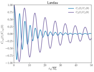
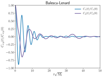
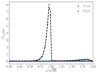
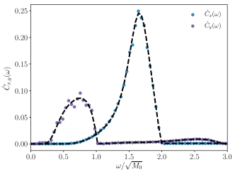
Figure 2: Correlation functions ${C_{x}(t)}$ and ${C_{y}(t)}$ (upper panels) and their Fourier transforms ${\widehat{C}_{x}(\omega)}$ and ${\widehat{C}_{y}(\omega)}$ (lower panels) for a non-interacting (Landau) bath (left) and a self-interacting (BL) bath (right) with magnetization ${M_{0}=0.816}$. In the lower panels, the dashed lines show ${\widehat{C}_{x}(\omega)}$ and ${\widehat{C}_{y}(\omega)}$ evaluated by equation (130).

In order to compare the measurements of correlations made via bath realizations, in Figure 2, we also represented a direct analytical calculation of the correlations ${\widehat{C}_{x}(\omega)}$ and ${\widehat{C}_{y}(\omega)}$. Indeed, following BM17, the Fourier transform of the correlation functions giving rise to the BL diffusion coefficients from equation (75) read

$$\widehat{C}_{x}(\omega)=\frac{2\pi}{N}\sum_{k>0}\sum_{\kappa^{\star}}\frac{|c_{k}(\kappa^{\star})|^{2}F_{\kappa}(\kappa^{\star})}{|\varepsilon_{cc}(k\Omega(\kappa^{\star}))|^{2}{|k\,\partial\Omega/\partial\kappa|}_{\kappa^{\star}}};\;\;\;\widehat{C}_{y}(\omega)=\frac{2\pi}{N}\sum_{n>0}\sum_{\kappa^{\star}}\frac{|s_{k}(\kappa^{\star})|^{2}\,F_{\kappa}(\kappa^{\star})}{|\varepsilon_{ss}(k\Omega(\kappa^{\star}))|^{2}{|k\,\partial\Omega/\partial\kappa|}_{\kappa^{\star}}},$$ (130)

where ${F_{\kappa}(\kappa)}$ is the PDF of $\kappa$. In equation (130), we also introduced the resonant locations $\kappa^{\star}$, which are the solutions of ${k\,\Omega(\kappa^{\star})=\omega}$. Finally, we also introduced the dressed susceptibility coefficients ${\varepsilon_{cc}(\omega)}$ and ${\varepsilon_{ss}(\omega)}$, capturing the amplitude of the self-gravitating amplification in the system. Following BM17, and as generically given by the response matrix from equation (139), these coefficients read

$$\varepsilon_{cc}(\omega)=1-2\pi\sum_{k}\!\!\int\!\!\mathrm{d}\kappa\,\frac{|c_{k}(\kappa)|^{2}\,k\,\partial F_{\mathrm{b}}/\partial\kappa}{\omega-k\Omega(\kappa)};\;\;\;\varepsilon_{ss}(\omega)=1-2\pi\sum_{k}\!\!\int\!\!\mathrm{d}\kappa\,\frac{|s_{k}(\kappa)|^{2}\,k\,\partial F_{\mathrm{b}}/\partial\kappa}{\omega-k\Omega(\kappa)}.$$ (131)

In the absence of collective effects, the susceptibility coefficients become ${\varepsilon_{cc}(\omega)=\varepsilon_{ss}(\omega)=1}$. Let us note that there are two main difficulties associated with the computation of the correlations from equation (130). First, in equation (130), one has to solve the non-local resonance condition, and determine the orbits $\kappa^{\star}$ that may resonate with a given frequency ${\omega/k}$. Moreover, this expression also involves the dressed susceptibility coefficients (see equation (131)), which ask for the delicate computation of an integral over orbital space exhibiting a pole at the resonance. While for the HMF model, equation (131) takes the form of a one-dimensional resonating integral, such expressions become more cumbersome to evaluate for inhomogeneous systems of higher dimensions (see e.g., Fouvry et al. (2015c) for ${2D}$ razor-thin disks). Let us finally recall that this analytical approach is made simpler for the HMF model, owing to the constraint from equation (124), which separates the $J$, $k$, and $t$ dependence in the potential fluctuations.

In Figure 2, we show that the computation of the noise correlation either from bath realizations or from analytical calculations both match. When the bath is self-interacting, Figure 2 illustrates also the result from equation (73). Indeed, for such a bath, provided one waits sufficiently for the correlation to build up, the fluctuations in the bath may be considered as being created by a non-interacting bath for which the pairwise interaction potential has been dressed, i.e. making the change ${\psi_{\mathbf{k}{\mathbf{k}^{\prime}}}(\mathbf{J},{\mathbf{J}^{\prime}})\to\psi_{\mathbf{k}{\mathbf{k}^{\prime}}}^{\mathrm{d}}(\mathbf{J},{\mathbf{J}^{\prime}},\omega)}$.

Following the characterization of the correlation of the fluctuations in Figure 2, it is then straightforward to compute the associated diffusion coefficients, as given by equation (48). The HMF diffusion coefficients are shown in Figure 3 as a function of $\overline{J}$, as introduced in equation (144).

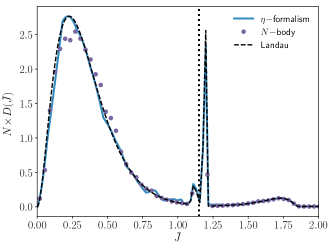
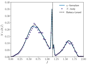
Figure 3: Diffusion coefficients for a non-interacting bath (left) and an self-interacting bath (right) with magnetization ${M_{0}=0.816}$, as a function of the rescaled action $\overline{J}$ (defined in equation (144)). The thick solid line shows the diffusion coefficients as obtained by the $\eta$-formalism, the dashed lines are obtained from equations (127) and (130), while the dots reproduce the direct measurements of the diffusion coefficients of BM17 performed from $N$-body simulations. The vertical dotted line indicates the location of the separatrix (i.e. ${\kappa=1}$).

In this figure, we show different methods to compute the diffusion coefficients. The first approach is based on the present $\eta$-formalism. As shown in Figure 2, it amounts to characterize the correlations of the fluctuations in the system, over many bath realizations. Once these perturbations are determined, the diffusion coefficients are immediately given by equation (127). As already computed in BM17, another approach is to compute the system’s dressed susceptibility coefficients, ${\varepsilon_{cc}(\omega)}$ and ${\varepsilon_{ss}(\omega)}$, from equation (131). Then, one may compute the correlation functions from equation (130), which immediately give the diffusion coefficients. Finally, we also reproduced in Figure 3 the data from BM17, obtained by measuring the diffusion coefficients directly from $N$-body simulations. As shown in Figure 3, all three approaches match, which illustrates the versatility of the $\eta$-formalism. Let us emphasize that, contrary to the analytical computation of the diffusion coefficients based on equation (130), the $\eta$-formalism approach does not ask for the resolution of the resonant condition ${k\Omega(\kappa)-{k^{\prime}}\Omega(\kappa^{\prime})=0}$, nor for the computation of the dressed susceptibility coefficients ${\varepsilon_{cc}(\omega)}$ and ${\varepsilon_{ss}(\omega)}$ from equation (131), which can all prove to be cumbersome in generic inhomogeneous self-gravitating systems. The only requirement of the $\eta$-formalism is to be able to perform bath realizations, either non- or self-interacting, from which the correlation of the potential perturbations can be characterized.

To finish this section, let us briefly discuss some of the features of the HMF diffusion coefficients presented in Figure 3. First, comparing the left and right panels, one cannot that even if the HMF pairwise interaction potential from equation (112) is attractive, this does not necessarily translate into the dressed (BL) diffusion coefficients being larger than the bare (Landau) ones. Here, for a HMF model with a large magnetization, collective effects tend to slow down the long-term diffusion. As shown in Figure 9 of BM17, should one consider a lower mean magnetization, this trend would invert and the BL diffusion coefficients would become larger than the Landau ones. In the case of razor-thin cold stellar discs, Fouvry et al. (2015c) similarly showed how self-gravity could hasten the long-term diffusion by at least three other of magnitudes.

In Figure 3, surrounding the separatrix, one can also note the presence of sharp peaks of enhanced diffusion. Such regions were not presented in BM17 and attributed to numerical instabilities of the computation near the separatrix (B. Marcos, private communication). Here we show that these peaks are not numerical artifacts, and are recovered in Figure 3 by all three methods. Their origin may be understood as follows. First, we note that these peaks are associated with orbits $\overline{J}$ with non vanishing orbital frequencies ${\Omega(\overline{J})}$. In that region of orbital space, the assumption of a dominating mean field motion in the Landau and BL equations therefore applies. Glancing back at the correlations represented in Figure 2, the origin of these peaks can be understood from the $\eta$-formalism. Indeed, as given by equation (145), at the separatrix, one has ${\Omega(\kappa=1)=0}$, and the frequency then grows very rapidly away from the separatrix. As a result, when moving away from the separatrix, the diffusion coefficient ${D(\overline{J})\propto\widehat{C}(\Omega(\overline{J}))}$ rapidly scans the peak of the correlations represented in Figure 2, leading to the narrow peaks observed in Figure 3. We finally note that the present formalism cannot be naively applied at the separatrix, as particles there have ${\Omega(\overline{J})\simeq 0}$, so that the assumption of having a fast orbital motion driven by the mean field potential does not apply there. Characterizing the properties of the stochastic diffusion at the separatrix requires therefore a more careful and elaborate study, which is beyond the scope of this work.

9 Conclusions

A long-range interacting system in which the mean field potential is integrable will evolve on the long-term due to the graininess of the potential associated with the finite number of particles. For such a system in the statistical limit ${N\gg 1}$, the long-term evolution of the integrals of motion (conveniently cast into actions $\mathbf{J}$) is stochastic and can be regarded as a diffusion process.

It is then enlightening to consider the evolution of one subject particle whose actions are undergoing a stochastic evolution sourced by the potential fluctuations. This evolution can be described by a diffusion equation containing a diffusion term and an advection (drift) term. The diffusion term results from the stochastic forces induced by the potential fluctuations of the $N$-body system of bath particles and is independent of the mass of the subject particle. The advection term results from the response of the system to the perturbation induced by the subject particle. As such, this advection term results from the wake created by the subject particle and gives rise to dynamical friction. Because the advection term is proportional to the mass of the subject particle, it vanishes in the limit where the mass of the subject particle is zero.

In this study, we presented a new approach, generalizing the so-called $\eta$-formalism (Bar-Or & Alexander, 2014), to derive the diffusion equation of a test particle forced by stochastic potential perturbations from bath particles. Assuming that the mean potential is integrable and that the bath orbits possess non-zero (and non-degenerate) orbital frequencies, the potential fluctuations in the bath can be treated as a general correlated Gaussian noise. In this work, we showed that the diffusion coefficients are proportional to the Fourier transform of the temporal correlation (i.e. spectral density) of the noise, evaluated at the test particle’s local orbital frequency ${\omega=\mathbf{k}\cdot\bm{\Omega}(\mathbf{J})}$ (see equation (48)). The calculation of the diffusion coefficients is therefore reduced to the task of obtaining the spectral density of the potential fluctuations generated by the bath. In the absence of additional simplifying assumptions, this spectral density can be obtained from numerical simulations.

One limit for which the correlation functions can be computed more easily is the limit in which the bath particles are assumed to be non-interacting, so that they are only driven by the mean field potential. This limit, which amounts to neglecting collective effects, is valid in particular when the mean field DF satisfies ${\partial F_{\mathrm{b}}(\mathbf{J})/\partial\mathbf{J}=0}$. This is for example relevant to describe the scalar resonant relaxation of three-dimensional isotropic quasi-Keplerian systems (Bar-Or & Alexander, 2014). We showed explicitly in equation (62), that in the limit of a non-interacting bath, the diffusion coefficients from the $\eta$-formalism are equivalent to the ones of the inhomogeneous Landau equation.

In the more general case where the bath particles can interact one with another, i.e. when accounting for collective effects, we showed in equation (75) that the $\eta$-formalism allows for a straightforward recovery of the inhomogeneous BL diffusion coefficients. These coefficients rely on the inversion of the self-consistency amplification relation in equation (70) defining the dressed susceptibility coefficients.

In Section 5, we lifted the assumption of treating the bath as external, and recovered the friction force by polarization associated with the back-reaction of the test particle on the bath particles’ motion. This allowed us to fully recover the Landau and BL equations in Section 6. Finally, in Section 7, we also briefly illustrated how the $\eta$-formalism allows for the recovery of the externally induced dressed diffusion coefficients previously obtained in Binney & Lacey (1988); Weinberg (2001a). These various diffusion equations are now being increasingly used to investigate complex regimes of long-term evolution of self-gravitating systems.

Finally, in order to emphasize the alternative point of view provided by the $\eta$-formalism, we illustrated in Section 8 how the $\eta$-formalism allows for the computation of the diffusion coefficients in the one-dimensional inhomogeneous HMF model. In particular, we showed how the characterization of the potential fluctuations makes it possible to determine the dressed susceptibility coefficients without having to invert their self-consistency definition from equation (70) required in the BL calculation.

Together with the BL equation, the $\eta$-formalism offers an equivalent but alternative framework, in which it is now possible to tackle the question of the long-term evolution of self-gravitating systems on a whole range of nested astrophysical systems. As an example, such methods may be used to investigate the long-term (scalar) resonant relaxation of galactic nuclei, generalizing the previous descriptions of Bar-Or & Alexander (2014, 2016).

Appendix A Initial correlations of the fluctuations

Following Chavanis (2012b), let us briefly characterize the statistical properties of the initial fluctuations in the DF of a bath composed of $N$ identical particles. As introduced in equation (53), the DF’s fluctuations are given by ${\delta F=F_{\mathrm{d}}-F_{\mathrm{b}}}$, where $F_{\mathrm{d}}$ is the discrete DF from equation (50) and $F_{\mathrm{b}}$ is the smooth mean field DF of the bath. To shorten the notations, we temporarily drop the time dependence, ${t=0}$. We can write

$$\left\langle\delta F(\bm{\theta},\mathbf{J})\,\delta F({\bm{\theta}^{\prime}},{\mathbf{J}^{\prime}})\right\rangle=m_{\mathrm{b}}^{2}\sum_{i,j}^{N}\left\langle\delta_{\mathrm{D}}(\bm{\theta}-\bm{\theta}_{i})\,\delta_{\mathrm{D}}(\mathbf{J}-\mathbf{J}_{i})\,\delta_{\mathrm{D}}({\bm{\theta}^{\prime}}-\bm{\theta}_{j})\,\delta_{\mathrm{D}}({\mathbf{J}^{\prime}}-\mathbf{J}_{j})\right\rangle-F_{\mathrm{b}}(\mathbf{J})\,F_{\mathrm{b}}({\mathbf{J}^{\prime}}),$$ (132)

where we relied on the fact that the fluctuations are of zero mean so that ${\left\langle\delta F\right\rangle=0}$. One can straightforwardly evaluate the first term from equation (132). It reads

$$m_{\mathrm{b}}^{2}\sum_{i,j}^{N}\left\langle\delta_{\mathrm{D}}(\bm{\theta}-\bm{\theta}_{i})\,\delta_{\mathrm{D}}(\mathbf{J}-\mathbf{J}_{i})\,\delta_{\mathrm{D}}({\bm{\theta}^{\prime}}-\bm{\theta}_{j})\,\delta_{\mathrm{D}}({\mathbf{J}^{\prime}}-\mathbf{J}_{j})\right\rangle={} m_{\mathrm{b}}^{2}\sum_{i}^{N}\left\langle\delta_{\mathrm{D}}(\bm{\theta}-\bm{\theta}_{i})\,\delta_{\mathrm{D}}(\mathbf{J}-\mathbf{J}_{i})\,\delta_{\mathrm{D}}(\bm{\theta}-{\bm{\theta}^{\prime}})\,\delta_{\mathrm{D}}(\mathbf{J}-{\mathbf{J}^{\prime}})\right\rangle$$

$$+m_{\mathrm{b}}^{2}\sum_{i\neq j}^{N}\left\langle\delta_{\mathrm{D}}(\bm{\theta}-\bm{\theta}_{i})\,\delta_{\mathrm{D}}(\mathbf{J}-\mathbf{J}_{i})\,\delta_{\mathrm{D}}({\bm{\theta}^{\prime}}-\bm{\theta}_{j})\,\delta_{\mathrm{D}}({\mathbf{J}^{\prime}}-\mathbf{J}_{j})\right\rangle$$

$$={} m_{\mathrm{b}}\,F_{\mathrm{b}}(\mathbf{J})\,\delta_{\mathrm{D}}(\bm{\theta}-{\bm{\theta}^{\prime}})\,\delta_{\mathrm{D}}(\mathbf{J}-{\mathbf{J}^{\prime}})+F_{\mathrm{b}}(\mathbf{J})\,F_{\mathrm{b}}({\mathbf{J}^{\prime}}),$$ (133)

where to obtain the last line, we assumed that the particles were initially uncorrelated and following equation (53) used the relation ${\left\langle F_{\mathrm{d}}\right\rangle\!=\!F_{\mathrm{b}}}$. Injecting equation (A) into equation (132), we immediately get

$$\left\langle\delta F(\bm{\theta},\mathbf{J})\,\delta F({\bm{\theta}^{\prime}},{\mathbf{J}^{\prime}})\right\rangle=m_{\mathrm{b}}\,F_{\mathrm{b}}(\mathbf{J})\,\delta_{\mathrm{D}}(\bm{\theta}-{\bm{\theta}^{\prime}})\,\delta_{\mathrm{D}}(\mathbf{J}-{\mathbf{J}^{\prime}}).$$ (134)

When Fourier transformed w.r.t. the angles, one finally gets the needed correlation of the initial fluctuations

$$\left\langle\delta F_{\mathbf{k}}(\mathbf{J},0)\,\delta F_{{\mathbf{k}^{\prime}}}({\mathbf{J}^{\prime}},0)\right\rangle=\frac{m_{\mathrm{b}}}{{(2\pi)}^{d}}\,\delta_{-\mathbf{k}{\mathbf{k}^{\prime}}}\,\delta_{\mathrm{D}}(\mathbf{J}-{\mathbf{J}^{\prime}})\,F_{\mathrm{b}}(\mathbf{J}).$$ (135)

Appendix B The basis method

In this Appendix, we briefly present the matrix method first introduced in Kalnajs (1976), which allows for an easier inversion of equation (68), which defines implicitly the dressed susceptibility coefficients. Let us introduce a representative biorthogonal basis of potentials and densities ${\psi^{(\alpha)}(\mathbf{x})}$ and ${\rho^{(\alpha)}(\mathbf{x})}$ satisfying

$$\psi^{(\alpha)}(\mathbf{x})=\!\!\int\!\!\mathrm{d}{\mathbf{x}^{\prime}}\,\psi(\mathbf{x},{\mathbf{x}^{\prime}})\,\rho^{(\alpha)}({\mathbf{x}^{\prime}})\;\;\;;\;\;\;\!\!\int\!\!\mathrm{d}\mathbf{x}\,\psi^{(\alpha)}(\mathbf{x})\,\rho^{(\beta)}(\mathbf{x})=-\delta_{\alpha\beta},$$ (136)

where once again, ${\psi(\mathbf{x},{\mathbf{x}^{\prime}})}$ is the pairwise interaction potential, i.e. ${\psi(\mathbf{x},{\mathbf{x}^{\prime}})\!=\!-G/|\mathbf{x}-{\mathbf{x}^{\prime}}|}$ in the gravitational context. These basis elements can then be used to represent the potential and density perturbations in the system. Following equation (7), we define the Fourier transform of the potential elements as

$$\psi_{\mathbf{k}}^{(\alpha)}(\mathbf{J})=\!\!\int\!\!\frac{\mathrm{d}\bm{\theta}}{{(2\pi)}^{d}}\,\psi^{(\alpha)}(\mathbf{x}[\bm{\theta},\mathbf{J}])\,\mathrm{e}^{-\mathrm{i}\mathbf{k}\cdot\bm{\theta}}.$$ (137)

These basis elements allow then for the explicit inversion of equation (70), which defines self-consistently the dressed susceptibility coefficients ${\psi_{\mathbf{k}{\mathbf{k}^{\prime}}}^{\mathrm{d}}(\mathbf{J},{\mathbf{J}^{\prime}},\omega)}$. Indeed, one has (see e.g., Chavanis (2012b))

$$\psi_{\mathbf{k}{\mathbf{k}^{\prime}}}^{\mathrm{d}}(\mathbf{J},{\mathbf{J}^{\prime}},\omega)=-\sum_{\alpha,\beta}\psi_{\mathbf{k}}^{(\alpha)}(\mathbf{J})\,{\big{[}\mathbf{I}-\widehat{\mathbf{M}}(\omega)\big{]}}_{\alpha\beta}^{-1}\,\psi_{{\mathbf{k}^{\prime}}}^{(\beta)}({\mathbf{J}^{\prime}}).$$ (138)

In equation (138), the sums over $\alpha$ and $\beta$ run over all the considered basis elements. In this equation, $\mathbf{I}$ is the identity matrix, while ${\widehat{\mathbf{M}}(\omega)}$ is the response matrix of the bath. It reads

$$\widehat{\mathbf{M}}_{\alpha\beta}(\omega)={(2\pi)}^{d}\sum_{\mathbf{k}}\!\!\int\!\!\mathrm{d}\mathbf{J}\,\frac{\mathbf{k}\!\cdot\!\partial F_{\mathrm{b}}/\partial\mathbf{J}}{\omega-\mathbf{k}\!\cdot\!\bm{\Omega}(\mathbf{J})}\,\psi_{\mathbf{k}}^{(\alpha)*}(\mathbf{J})\,\psi_{\mathbf{k}}^{(\beta)}(\mathbf{J}).$$ (139)

In the limit where collective effects are not accounted for, equation (138) recovers the expression of the bare susceptibility coefficients reading

$$\psi_{\mathbf{k}{\mathbf{k}^{\prime}}}(\mathbf{J},{\mathbf{J}^{\prime}})=-\sum_{\alpha}\psi_{\mathbf{k}}^{(\alpha)}(\mathbf{J})\,\psi_{{\mathbf{k}^{\prime}}}^{(\alpha)*}({\mathbf{J}^{\prime}}).$$ (140)

The response matrix $\widehat{\mathbf{M}}$ is an essential dynamical quantity that characterizes the properties of the self-gravitating amplification of perturbations in the bath. As an example, the bath is linearly unstable if there exists $\omega$ with ${\text{Im}[\omega]>0}$, such that ${\det[\mathbf{I}-\widehat{\mathbf{M}}(\omega)]=0}$. One should note from equation (139), that the response matrix is a global mean field quantity, in the sense that it only depends on the mean field properties of the bath (via $F_{\mathrm{b}}$ and ${\bm{\Omega}(\mathbf{J})}$) and involves an integration over all action space. As such, numerical calculations of unstable modes of self-gravitating systems are cumbersome tasks. In astrophysics, it has only been made for a small number of razor-thin disks (see e.g., Zang, 1976; Kalnajs, 1977; Vauterin & Dejonghe, 1996; Pichon & Cannon, 1997; Evans & Read, 1998; Jalali & Hunter, 2005; Polyachenko, 2005; Jalali, 2007, 2010; Fouvry et al., 2015c; De Rijcke & Voulis, 2016) or three-dimensional spherical clusters (see e.g., Polyachenko & Shukhman, 1981; Saha, 1991; Weinberg, 1991).

Appendix C Angle-action coordinates for the HMF model

In this Appendix, we follow Barré et al. (2010); Benetti & Marcos (2017) and present angle-action coordinates for the inhomogeneous HMF model considered in Section 8. Let us first introduce the quantity $\kappa$ conserved for the mean field dynamics

$$\kappa=\sqrt{\frac{H_{\mathrm{t}}\!+\!M_{0}}{2M_{0}}},$$ (141)

where the one-particle Hamiltonian, $H_{\mathrm{t}}$, stands for the specific energy of the particle, and was introduced in equation (113). The quantity $\kappa$ is a useful parameter to separate the librating particles from the circulating ones. The separatrix lies in ${\kappa=1}$, so that particles with ${\kappa<1}$ are trapped and librate, while particles with ${\kappa>1}$ are circulating. The action $J$ may then be defined as

$$J(\kappa)=\frac{4\sqrt{M_{0}}}{\pi}\begin{cases}\displaystyle 2[E(\kappa^{2})-(1\!-\!\kappa^{2})K(\kappa^{2})]\;\;\;\text{if}\;\;\;\kappa<1,\\ \displaystyle\kappa E(1/\kappa^{2})\;\;\;\text{if}\;\;\;\kappa>1.\end{cases}$$ (142)

In equation (142), we introduced the complete elliptic integrals of the first and second kind, ${K(m)}$ and ${E(m)}$, with the convention

$$K(m)=\!\!\int_{0}^{\pi/2}\!\!\!\!\mathrm{d}x\,{\big{[}1\!-\!m\sin^{2}(x)\big{]}}^{-1/2}\;\;\;;\;\;\;E(m)=\!\!\int_{0}^{\pi/2}\!\!\!\!\mathrm{d}x\,{\big{[}1\!-\!m\sin^{2}(x)\big{]}}^{1/2}.$$ (143)

In equation (142), one should pay attention to the fact that the action $J$ is discontinuous at the separatrix ${\kappa\!=\!1}$. To avoid this issue, we introduce a rescaled action $\overline{J}$ as

$$\overline{J}=\begin{cases}J/2&\kappa<1,\\ J&\kappa>1.\end{cases}$$ (144)

Finally, the orbital frequency ${\Omega(\kappa)}$ is given by

$$\Omega(\kappa)=\pi\sqrt{M_{0}}\begin{cases}\displaystyle 1/(2K(\kappa^{2}))\;\;\;\text{if}\;\;\;\kappa<1,\\ \displaystyle\kappa/(K(1/\kappa^{2}))\;\;\;\text{if}\;\;\;\kappa>1.\end{cases}$$ (145)

In equation (128), we assumed that the quasi-stationary DF of the bath takes the form of a thermal DF that can be written as

$$F_{0}(\kappa)=C\,\exp\big{[}-\beta M_{0}(2\kappa^{2}\!-\!1)\big{]}\;\;\;\text{with}\;\;\;C=\sqrt{\frac{\beta}{{(2\pi)}^{3}}}\frac{1}{I_{0}(\beta M_{0})},$$ (146)

In equation (146), the DF satisfies the normalization convention ${\!\!\int\!\!\mathrm{d}\theta\mathrm{d}JF_{0}(J)\!=\!M\!=\!1}$. We also introduced the inverse temperature $\beta$ which is determined self-consistently from the mean magnetization $M_{0}$ by imposing ${\{\cos(\phi)\}\!=\!M_{0}}$, so that one has

$$M_{0}=\frac{I_{1}(\beta M_{0})}{I_{0}(\beta M_{0})}.$$ (147)

The explicit angle-action coordinates from equation (142) allow us to perform the needed Fourier transforms w.r.t. the angle $\theta$. Following Benetti & Marcos (2017), these are characterized by two quantities ${c_{k}(\kappa)}$ and ${s_{k}(\kappa)}$ defined as

$$c_{k}(\kappa)=\!\!\int_{-\pi}^{\pi}\!\frac{\mathrm{d}\theta}{2\pi}\,\cos[\phi(\theta,\kappa)]\,\mathrm{e}^{-\mathrm{i}k\theta}\;\;\;;\;\;\;s_{k}(\kappa)=\!\!\int_{-\pi}^{\pi}\!\frac{\mathrm{d}\theta}{2\pi}\,\sin[\phi(\theta,\kappa)]\,\mathrm{e}^{-\mathrm{i}k\theta}.$$ (148)

Fortunately, these integrations can be performed explicitly and one gets

$$c_{k}(\kappa)=\begin{cases}\begin{aligned} &\frac{\pi^{2}}{K^{2}(\kappa^{2})}\frac{|k|\,{q(\kappa^{2})}^{|k|/2}}{1\!-\!{q(\kappa^{2})}^{|k|}}&&\kappa<1,\;k\;\text{even},\\ &0&&\kappa<1,\;k\;\text{odd},\\ &\frac{2\pi^{2}\kappa^{2}}{K^{2}(1/\kappa^{2})}\frac{|k|\,{q(1/\kappa^{2})}^{|k|}}{1-{q(1/\kappa^{2})}^{2|k|}}&&\kappa>1,\end{aligned}\end{cases}\!\!\!;\;s_{k}(\kappa)=\begin{cases}\begin{aligned} &0&&\kappa<1,\;k\;\text{even},\\ &-\mathrm{i}\frac{\pi^{2}}{K^{2}(\kappa^{2})}\frac{k\,{q(\kappa^{2})}^{|k|/2}}{1+{q(\kappa^{2})}^{|k|}}&&\kappa<1,\;k\;\text{odd},\\ &-\mathrm{i}\frac{2\pi^{2}\kappa^{2}}{K^{2}(1/\kappa^{2})}\frac{k\,{q(1/\kappa^{2})}^{|k|}}{1+{q(1/\kappa^{2})}^{2|k|}}&&\kappa>1,\;v>0,\\ &\mathrm{i}\frac{2\pi^{2}\kappa^{2}}{K^{2}(1/\kappa^{2})}\frac{k\,{q(1/\kappa^{2})}^{|k|}}{1+{q(1/\kappa^{2})}^{2|k|}}&&\kappa>1,\;v<0,\end{aligned}\end{cases}$$ (149)

where ${q(m)\!=\!\exp[-\pi K(1\!-\!m)/K(m)]}$ is the elliptic nome. The coefficients ${c_{k}(J)}$ and ${s_{k}(J)}$ are the ones appearing in equation (124) to describe the noise induced by the bath.

Finally, following Brizard (2013), one can integrate explicitly the motion of a given particle when driven by the mean field HMF potential. Such explicit time integrations are used in Section 8 to characterize the fluctuations of the magnetization in a non-interacting HMF bath. Let us first consider a trapped particle, i.e. for which ${\kappa<1}$, characterized by the initial coordinates ${(\phi_{0},v_{0})}$. We introduce $\varepsilon_{0}$ as

$$\varepsilon_{0}=\text{sign}[v_{0}],$$ (150)

and the phase of the pendulum ${\phi_{\mathrm{P}}}$ as

$$\phi_{\mathrm{P}}=\varepsilon_{0}\,\text{sn}^{-1}\big{[}\sin(\phi_{0}/2)/\kappa,\kappa^{2}\big{]}.$$ (151)

In equation (151), we defined the inverse Jacobi elliptic function ${\text{sn}^{-1}(u,m)}$ with the convention

$$\text{sn}[u\,,\,m]=\sin(\varphi)\;\;\;\text{with}\;\;\;\varphi=\text{am}[u\,,\,m]\;\;;\;\;u=F[\varphi\,,\,m]=\!\!\int_{0}^{\varphi}\!\!\mathrm{d}\vartheta\,{\big{[}1\!-\!m\sin^{2}(\vartheta)\big{]}}^{-1/2}.$$ (152)

The motion of a librating particle can then be explicitly integrated in time and reads

$$\phi(t)=\varepsilon_{0}\,2\,\text{Arcsin}\big{[}\kappa\,\text{sn}\big{[}\phi_{\mathrm{P}}+t\sqrt{M_{0}}\,,\,\kappa^{2}\big{]}\big{]}.$$ (153)

For a circulating orbit, i.e. with ${\kappa>1}$, similarly to equations (150) and (151), we introduce ${\varepsilon_{0}}$ and ${\phi_{\mathrm{P}}}$ as

$$\varepsilon_{0}=\text{sign}[v_{0}]\;\;\;;\;\;\;\phi_{\mathrm{P}}=\varepsilon_{0}\,\text{sn}^{-1}\big{[}\sin(\phi_{0}/2),1/\kappa^{2}\big{]}/\kappa.$$ (154)

We also introduce the times $t_{0}$ and the period ${\Delta t}$ as

$$t_{0}=\frac{1}{\sqrt{M_{0}}}\bigg{(}\frac{\text{sn}^{-1}\big{[}1,1/\kappa^{2}\big{]}}{\kappa}-\phi_{\mathrm{P}}\bigg{)}\;\;\;;\;\;\;\Delta t=\frac{2\,K[1/\kappa^{2}]}{\sqrt{M_{0}}\kappa},$$ (155)

where, following equation (152), we introduced the complete elliptic function ${K[m]=F[\pi/2,m]}$. The motion of the circulating particle can then be explicitly integrated in time and reads

$$\phi(t)=\begin{cases}\displaystyle\varepsilon_{0}\,2\,\text{Arcsin}\big{[}\text{sn}\big{[}\kappa(\phi_{\mathrm{P}}+t\sqrt{M_{0}}),1/\kappa^{2}\big{]}\big{]}\;\;\;\text{if}\;\;\;\text{Mod}\big{[}t-t_{0},2\Delta t\big{]}-\Delta t\leq 0,\\ -\varepsilon_{0}\,2\,\text{Arcsin}\big{[}\text{sn}\big{[}\kappa(\phi_{\mathrm{P}}+t\sqrt{M_{0}}),1/\kappa^{2}\big{]}\big{]}\;\;\;\text{otherwise},\displaystyle\end{cases}$$ (156)

with ${\text{Mod}[x,y]\!=\!y\,\text{frac}(x/y)}$. The explicit expressions from equations (153) and (156) allow us to easily perform realizations of non-interacting HMF bath, as presented in Section 8.

References

- Alexander (2015) Alexander T., 2015, preprint, (arXiv:1505.04823)
- Antoni & Ruffo (1995) Antoni M., Ruffo S., 1995, Phys. Rev. E, 52, 2361
- Bar-Or & Alexander (2014) Bar-Or B., Alexander T., 2014, Class. Quantum Grav., 31, 244003
- Bar-Or & Alexander (2016) Bar-Or B., Alexander T., 2016, ApJ, 820, 129
- Bar-Or et al. (2013) Bar-Or B., Kupi G., Alexander T., 2013, ApJ, 764, 52
- Barré et al. (2010) Barré J., Olivetti A., Yamaguchi Y. Y., 2010, J. Stat. Mech. Theor. Exp., 8, 08002
- Benetti & Marcos (2017) Benetti F. P. C., Marcos B., 2017, Phys. Rev. E, 95, 022111
- Binney & Lacey (1988) Binney J., Lacey C., 1988, MNRAS, 230, 597
- Binney & Tremaine (2008) Binney J., Tremaine S., 2008, Galactic Dynamics: Second Edition. Princeton University Press
- Brizard (2013) Brizard A. J., 2013, Commun. Nonlinear. Sci. Numer. Simul., 18, 511
- Campa et al. (2009) Campa A., Dauxois T., Ruffo S., 2009, Phys. Rep., 480, 57
- Chandrasekhar (1942) Chandrasekhar S., 1942, Principles of Stellar Dynamics. University of Chicago Press
- Chandrasekhar (1943) Chandrasekhar S., 1943, ApJ, 97, 255
- Chavanis (2012a) Chavanis P.-H., 2012a, Eur. Phys. J. Plus, 127, 19
- Chavanis (2012b) Chavanis P.-H., 2012b, Physica A, 391, 3680
- Chavanis (2013) Chavanis P.-H., 2013, A&A, 556, A93
- De Rijcke & Voulis (2016) De Rijcke S., Voulis I., 2016, MNRAS, 456, 2024
- Evans & Read (1998) Evans N. W., Read J. C. A., 1998, MNRAS, 300, 106
- Fouvry et al. (2015a) Fouvry J.-B., Pichon C., Prunet S., 2015a, MNRAS, 449, 1967
- Fouvry et al. (2015b) Fouvry J.-B., Pichon C., Chavanis P.-H., 2015b, A&A, 581, A139
- Fouvry et al. (2015c) Fouvry J.-B., Pichon C., Magorrian J., Chavanis P.-H., 2015c, A&A, 584, A129
- Fouvry et al. (2017a) Fouvry J.-B., Pichon C., Chavanis P.-H., 2017a, preprint, (arXiv:1705.01131)
- Fouvry et al. (2017b) Fouvry J.-B., Pichon C., Chavanis P.-H., Monk L., 2017b, MNRAS, 471, 2642
- Fouvry et al. (2017c) Fouvry J.-B., Pichon C., Magorrian J., 2017c, A&A, 598, A71
- Garcia-Ojalvo & Sancho (1999) Garcia-Ojalvo J., Sancho J., 1999, Noise in Spatially Extended Systems. Springer New York
- Heyvaerts (2010) Heyvaerts J., 2010, MNRAS, 407, 355
- Heyvaerts et al. (2017) Heyvaerts J., Fouvry J.-B., Chavanis P.-H., Pichon C., 2017, MNRAS, 469, 4193
- Hopman & Alexander (2006) Hopman C., Alexander T., 2006, ApJ, 645, 1152
- Jalali (2007) Jalali M. A., 2007, ApJ, 669, 218
- Jalali (2010) Jalali M. A., 2010, MNRAS, 404, 1519
- Jalali & Hunter (2005) Jalali M. A., Hunter C., 2005, ApJ, 630, 804
- Kalnajs (1976) Kalnajs A. J., 1976, ApJ, 205, 745
- Kalnajs (1977) Kalnajs A. J., 1977, ApJ, 212, 637
- Klimontovich (1967) Klimontovich I., 1967, The statistical theory of non-equilibrium processes in a plasma. M.I.T. Press
- Kocsis & Tremaine (2011) Kocsis B., Tremaine S., 2011, MNRAS, 412, 187
- Kocsis & Tremaine (2015) Kocsis B., Tremaine S., 2015, MNRAS, 448, 3265
- Luciani & Pellat (1987) Luciani J. F., Pellat R., 1987, J. Phys., 48, 591
- Lynden-Bell (1994) Lynden-Bell D., 1994, Lectures on stellar dynamics. Berlin Springer Verlag
- Lynden-Bell & Kalnajs (1972) Lynden-Bell D., Kalnajs A. J., 1972, MNRAS, 157, 1
- Merritt et al. (2011) Merritt D., Alexander T., Mikkola S., Will C. M., 2011, Phys. Rev. D, 84, 044024
- Mynick (1988) Mynick H. E., 1988, J. Plasma Phys., 39, 303
- Nardini et al. (2012) Nardini C., Gupta S., Ruffo S., Dauxois T., Bouchet F., 2012, J. Stat. Mech. Theor. Exp., 12, 12010
- Nelson & Tremaine (1999) Nelson R. W., Tremaine S., 1999, MNRAS, 306, 1
- Novikov (1965) Novikov E. A., 1965, Sov. Phys. JETP, 20, 1290
- Pichon (1994) Pichon C., 1994, Ph.D. thesis. University of Cambridge
- Pichon & Aubert (2006) Pichon C., Aubert D., 2006, MNRAS, 368, 1657
- Pichon & Cannon (1997) Pichon C., Cannon R. C., 1997, MNRAS, 291, 616
- Polyachenko (2005) Polyachenko E. V., 2005, MNRAS, 357, 559
- Polyachenko & Shukhman (1981) Polyachenko V. L., Shukhman I. G., 1981, Soviet Ast., 25, 533
- Polyachenko & Shukhman (1982) Polyachenko V. L., Shukhman I. G., 1982, Soviet Ast., 26, 140
- Rauch & Tremaine (1996) Rauch K. P., Tremaine S., 1996, New Astron., 1, 149
- Saha (1991) Saha P., 1991, MNRAS, 248, 494
- Seguin & Dupraz (1994) Seguin P., Dupraz C., 1994, A&A, 290, 709
- Spitzer (1987) Spitzer L., 1987, Dynamical evolution of globular clusters. Princeton University Press
- Sridhar & Touma (2016a) Sridhar S., Touma J. R., 2016a, MNRAS, 458, 4129
- Sridhar & Touma (2016b) Sridhar S., Touma J. R., 2016b, MNRAS, 458, 4143
- Sridhar & Touma (2017) Sridhar S., Touma J. R., 2017, MNRAS, 465, 1856
- Toomre (1981) Toomre A., 1981, in Fall S. M., Lynden-Bell D., eds, Structure and Evolution of Normal Galaxies. pp 111–136
- Tremaine & Weinberg (1984) Tremaine S., Weinberg M. D., 1984, MNRAS, 209, 729
- Vauterin & Dejonghe (1996) Vauterin P., Dejonghe H., 1996, A&A, 313, 465
- Weinberg (1989) Weinberg M. D., 1989, MNRAS, 239, 549
- Weinberg (1991) Weinberg M. D., 1991, ApJ, 368, 66
- Weinberg (1993) Weinberg M. D., 1993, ApJ, 410, 543
- Weinberg (2001a) Weinberg M. D., 2001a, MNRAS, 328, 311
- Weinberg (2001b) Weinberg M. D., 2001b, MNRAS, 328, 321
- Zang (1976) Zang T. A., 1976, Ph.D. thesis. Massachusetts Institute of Technology