Permeability of porous foamy materials

Abstract

In this paper, we study the effects of both the amount of open cell walls and their aperture sizes on solid foams permeability. FEM flow simulations are performed at both pore and macroscopic scales. For foams with fully interconnected pores, we obtain a robust power-law relationship between permeability and membrane aperture size. This result owns to the local pressure drop mechanism through the membrane aperture as described by Sampson for fluid flow through a circular orifice in a thin plate. Based on this local law, pore-network simulation of simple flow is used and is shown to reproduce successfully FEM results. This low computational cost method allowed to study in detail the effects of the open wall amount on percolation, percolating porosity and permeability. A model of effective permeability is proposed and shows ability to reproduce the results of network simulations. Finally, an experimental validation of the theoretical model on well controlled solid foam is presented.

I introduction

Foams are dispersions of gas in liquid or solid matrices. In liquid foams, the structure of foams is made of membranes (liquid films separating neighbor bubbles, also called walls), ligaments or Plateau’s borders (junction of three membranes) and vertex (junction of four ligaments). Contrary to liquid foam, in which membranes are necessary to ensure the stability of the foam, membranes can be partially or totally open in solid foams.

Permeability is a physical parameter that is used in many domains, such as geophysics, soil mechanics, petroleum engineering, civil engineering and acoustics of noise absorbing materials (e.g. polymeric foams). As viscous dissipation is the most dissipative mechanism in the sound propagation through porous materials, permeability (or flow resistivity) is a key parameter governing the acoustical properties of such materials (Johnson et al., 1987; Allard and Atalla, 2009). Different works have focused on the effects of foams geometry on permeability: amount of closed walls (Doutres et al., 2013), aperture of walls (Hoang and Perrot, 2012), solid volume fraction and ligament shapes (Kumar and Topin, 2017; Lusso and Chateau, ). Authors deduce some relations between permeability and studied parameters: solid volume fraction, size of aperture,… These relations take into account mechanisms acting at the scale of a bubble without taking into account percolation. Indeed, in porous media, below a critical concentration of bonds between pores inside a sample, the size of the interconnected porosity is smaller than the sample height and no flow through sample is possible. The classical Kozeny-Carman equation has to be modified to take into account such percolation, e.g. in substituting the porosity by the difference between the porosity and the critical porosity leading to percolation (Mavko and Nur, 1997). Similary in foamy porous materials, beyond a critical proportion of open walls, percolation has to occur. Moreover, in the vicinity of the percolation, a small part of pores is interconnected and the geometry of the pore network is complex. To study more precisely the mesoscopic effect of the pore network on permeability, numerical simulations should use large samples involving a few hundred bubbles. However, as the size of samples increases, the computational costs in FEM simulations become prohibitive. To overcome similar difficulties in simulations of flow through porous media, multi-scale approaches have been proposed (Kirkpatrick, 1973; Vogel, 2000; Marcke et al., 2010; Jivkov et al., 2013; Xiong et al., 2015, 2016): at the scale of a throat between two linked pores, the relationship between the flow rate passing through the throat linking pores and the difference of pressure between pores is determined by numerical simulations or analytical solutions (e.g. Hagen-Poiseuille equation); at the macro-scale, pore-network simulations are performed to determine the macroscopic permeability from local permeabilities found at the local scale (Fatt, 1956). In this paper, we have attempted to use a similar multi-scale approach to study the permeability of foamy media.

Different numerical simulations are performed at different scales to study the effect of aperture size and amount of closed walls. The effect of the aperture size on partially open cell foam is studied by using FEM simulations on periodic unit cells (PUC) involving the Kelvin partition of space and containing two pores. To study the effect of the proportion of closed walls, FEM simulations on larger samples containing 256 pores are carried out in order to produce a flow at the macroscopic scale and to simulate the complex flow through the porous network. The mesoscopic effects induced by the structure of the pore network are studied by pore-network simulations on large (up to 2000 pores) lattice networks of interconnected pores interacting via local permeabilities. A model of effective permeability based on a calculation of the mean local permeability as in Kirkpatrick (1973) is used to describe the percolation threshold and the effect of mixing local permeabilities. Finally, experimental measurements of permeability performed on polymeric foams are compared to the model predictions.

II numerical simulations of foam permeability

II.1 FEM Simulations of fluid flow

At the pore scale:

As shown on Fig. 1, a periodic unit cell containing two pores of size $D_{b}$ is used to represent the pore structure in foam samples (Perrot et al., 2007). The cell is based on the Kelvin paving and is a 14-sided polyhedron corresponding to 8 hexagons and 6 squares. The cell skeleton is made of idealized ligaments having length $L=D_{b}/(2\sqrt{2})$ and an equilateral triangular cross section of edge side $r=0.58D_{b}(1-\phi)^{0.521}$, where $\phi$ is the gas volume fraction (Cantat et al., 2013). In the reference configuration (Fig. 1a), the 14 cell windows are fully open (i.e. without wall). As we are interested in the effect of partial closure of the cell walls, we partially close the windows by adding walls characterized with distinct circular aperture sizes. Two kinds of simulations have been performed: (i) identical aperture size on all windows (Fig. 1b), (ii) identical rate of aperture $\delta_{ow}=t_{o}/t_{w}$ (Fig. 1c) where $t_{w}$ and $t_{o}$ are respectively the window size and the size of the wall aperture as defined in Fig. 1d. The static viscous permeability $K$ is computed from the solution of Stokes problem (Adler, 1992) for various porosity. The boundary value problem is solved by using the finite element method (at convergence, the mesh contains 214 412 tetrahedral elements) and the commercial software COMSOL Multiphysics.

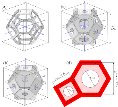
Figure 1: PUC without walls (a), with identical aperture size inside walls (b), with identical aperture rate (c), definitions of the aperture size $t_{o}$ and the window size $t_{w}$ (d).

At the macroscopic scale:

In order to study the flow properties on a larger scale, we have performed numerical simulation for the flow of a Newtonian fluid through a periodic network of Kelvins cells having a size $L\times L\times H=4\sqrt{2}\times 4\sqrt{2}\times 4$ in $D_{b}$ units (i.e. containing 256 pores), and a porosity$\phi$ equal to 0.9. Figure 2 shows an open cell foam sample made of 32 pores (i.e. all the windows between adjacent cells are open). The macroscopic intrinsic permeablity is computed from the averaging of the solution of a Stokes problem set on the foam sample. In this study, the cell windows are either closed or open with random spatial distribution over the foam sample. For each value of the proportion of open windows, the macroscopic intrinsic permeability is the average of numerical simulations for 6 different samples. The resolution of the boundary value problem is achieved through the Finite Element Method using FreeFem++ Software. Typical discrete problem contains 1 400 000 Tetrahedra and 8 000 000 degrees of freedom and is solved using a Message passing Interface (MPI) on 4 processors.

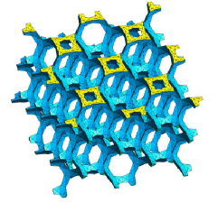
(a)(b)

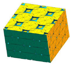
Figure 2: FEM macro-scale samples: skeleton mesh (a) and porosity mesh (b). For sake of visibility, a mesh of size $2\sqrt{2}\times 2\sqrt{2}\times 2$ ($D_{b}$ units) is depicted in this figure.

II.2 Pore-network simulations:

Effects of pore network features on permeability are studied on several lattices of size $L\times L\times H=10\times 10\times 10$ ($D_{b}$ units) having different maximal numbers of neighbor pores $N_{v}$ (Fig. 3). In the case $N_{v}=14$, samples contain 2000 pores and the structure of pores corresponds to Kelvin’s structure. Boundary effects are avoided by resorting to periodic conditions imposed in the directions perpendicular to the macroscopic flow. In this simple model, we consider, for each pore, a unique value of pressure without calculating the fluctuations of pressure and fluid velocity inside the pore. At the local scale, the flow rate $q_{j\rightarrow i}$ from pore $j$ to pore $i$ is governed by the differential pressure between the pores $\Delta P_{ij}=P_{j}-P_{i}$:

$q_{j\rightarrow i}=\frac{D_{b}}{\mu}k_{ij}\Delta P_{ij}$

where the coefficient $k_{ij}$ is the local permeability between the pores $i$ and $j$.

At steady state and by considering incompressible fluid, the volume of fluid inside pore $i$ is constant and the sum of flow rates coming from neighbor bubbles is equal to zero, leading to: $\sum_{j=1}^{N_{v}}k_{ij}\left(P_{j}-P_{i}\right)=0$. To generate a flow through the sample, a pressure difference is imposed between top and bottom faces of the sample ($P_{top}=\text{$\Delta$}P_{sp}$, $P_{bot}=0$). By considering these boundary conditions, this previous equation can take a matrix form:

$$\underline{K}\left[P_{i}\right]=\left[S_{i}\right]$$ (1)

where $\left[P_{i}\right]$ is a vector containing the pressure of inner pores (pores located on top and bottom faces are excluded); $\underline{K}$ is the matrix defined from local permeabilities ($-\sum k_{ij}$ along diagonal and $k_{ij}$ elsewhere) and $\left[S_{i}\right]$ is a vector containing zeros except for inner pores having top pores as neighbors where $S_{i}=-\sum_{j_{top}}k_{ij_{top}}\text{$\Delta$}P_{sp}$.

As soon as the pore network links top to bottom and by considering only the interconnected pores, $\underline{K}$ can be inverted and the fluid pressure in each pore can be calculated from Eq.1. Therefore, the macroscopic flow $Q$ and the macro permeability $K$ can be calculated as follows:

$Q=\sum_{i_{bot}}\sum_{j_{v}}q_{j_{v}\rightarrow i_{bot}}=\frac{D_{b}}{\mu}\sum_{i_{bot},j_{vi}}k_{i_{bot}j_{vi}}\Delta P_{i_{bot},j_{vi}}$

$K=\mu QH/L^{2}\text{$\Delta$}P_{sp}$

Different materials having different kinds of local permeability distribution have been studied: two local permeabilities (binary mixture), a local permeability mixed with zero permeability (closed walls) and two local permeabilities mixed with closed walls. For each kind of local permeability distribution, calculations are repeated from 200 to 400 times on different random draws in order to calculate an average. For each random draw, local permeabilities are randomly distributed over the network.

Figure 3: Network structures used in network simulations.

II.3 Results and discussion

Effect of the aperture size

FEM simulations on PUC at the pore scale for various aperture sizes reveal a power-law relationship between permeability and aperture size (Fig.4a). Similarly the numerical results for the dimensionless permeability of porous materials with same aperture rate are well fitted by a power law when plotted in a ($\delta_{ow}$, $K/D_{b}^{2}$) diagram (Fig.4b). Note that, for high aperture rates, the condition of identical aperture rate is not observed due to the fact that the apertures should overlap the ligaments, which is not allowed in our calculations. This artifact leads to an artificial permeability plateau corresponding to the “no wall” permeability. Apart from this artifact, FEM results show that relationship between permeability and mean wall aperture is almost unaffected by the porosity (i.e. the width of ligaments).

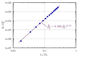
(a)(b)
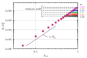
(c)

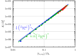
Figure 4: (a) FEM results at identical aperture size with $\phi=0.98$, (b) FEM results at identical aperture rate for various $\phi$, (c) Permeability as a function of the mean wall apertures: FEM results (blue dot for identical aperture, green dot for identical rate, red cross for “no wall” foam with $\phi$ varying from 0.8 to 0.99), network simulation with Sampson local permeabilities and $N_{v}=14$ (blue line for identical aperture, green line for identical rate). Note that the mean wall aperture is calculated without including the four square windows which are parallel to the macroscopic flow direction $\left\langle t_{o,eq}\right\rangle/D_{b}=(2t_{o,sq}+8t_{o,hex})/10D_{b}.$

This power-law relationship is in agreement with a local interpretation based on the pressure drop of the fluid passing through the wall aperture. Indeed, Sampson (Sampson, 1891) solves analytically the problem of the pressure drop $\Delta P$ occurring for an incompressible fluid flow passing through a circular hole of diameter $d_{o}$ in a thin plate:

$$\frac{Q}{\Delta P}=\frac{d_{o}^{3}}{24\mu}$$ (2)

where $Q$ is the volume fluid flow rate passing through the hole and $\mu$ is the fluid dynamic viscosity.

This relation arises from the fact that, at low Reynolds number, the coefficient of fluid resistance $\zeta=2\Delta P/(\rho V_{o}^{2})$ is in general, proportional to the inverse of Reynolds number $R_{e}=V_{o}d_{o}\rho/\mu$ (Idel’Cik, 1996), where $V_{o}$ is the mean stream velocity in the narrowest section of the orifice ($V_{o}=4Q/\pi d_{o}^{2}$).

After (van Melick and Geurts, 2013), the pressure drop through a hole of circular shape is very close to the one obtained with a hole of squared shape having the same area. We can deduce that the Sampson formula can be extended to squared and hexagonal shape of aperture by taken into account an equivalent diameter $t_{o,eq}$ defined from the surface area of the aperture $S_{o}$: $t_{o,eq}=2(S_{o}/\pi)^{0.5}$. By using such a definition for the aperture size and calculating a window average of the aperture size, we can plot all FEM results on a same graph. Fig. 4c shows that all data, including the ones obtained without wall, follow the same trend. Therefore, due to the peculiar pore geometry of foams, the pressure drop inside such porous materials is governed by a local mechanism which is not described by the usual Hagen-Poiseuille equation as it is done in classical porous media (Fatt, 1956; Vogel, 2000; Jivkov et al., 2013; Xiong et al., 2015).

To check the ability of pore-network model to predict the permeability, network calculations have been performed using local permeabilities given by a Sampson equation:

$$k=t_{0}^{3}/24D_{b}$$ (3)

In such simple simulated configurations (i.e. identical aperture size or identical aperture rate), the network problem exposed in the previous section can be solved analytically. Therefore, macroscopic permeability is given by $K=2k_{sq}+2k_{hex}$, leading to $\frac{K}{D_{b}^{2}}=\frac{1}{6}\left(\frac{t_{0}}{D_{b}}\right)^{3}$ for identical aperture size and $\frac{K}{D_{b}^{2}}=\frac{1+3^{1.5}}{12}\left(\frac{5}{1+48^{0.5}}\frac{\left\langle t_{o,eq}\right\rangle}{D_{b}}\right)^{3}\approx 0.13\left(\frac{\left\langle t_{o,eq}\right\rangle}{D_{b}}\right)^{3}$ for identical aperture rate. Fig. 4c shows that network simulation results compare very well to FEM results. This good agreement supports both the interpretation of the permeability by using local permeabilities and the relevance of pore-network simulations.

Effect of closed walls

Fig. 5 shows the permeabilities calculated by FEM simulations on large samples having random positions of closed walls and various open walls fractions $x_{ow}$ (defined as the number of open wall over the total number of walls in the porous sample). For $x_{ow}>0.3$, permeability exhibits a quasi-affine dependence on the open walls fraction $x_{ow}$. Below a critical concentration $x_{ow}<0.2$, the fluid flow vanishes.

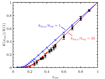
Figure 5: Dimensioless permeability $K(x_{ow})/K(1)$ as a function of open walls fraction $x_{ow}$ for FEM simulations (black square) and network simulations on samples mixing two local permeabilities with various ratios $k_{hex}/k_{sq}$ and having a Kelvin structure ($N_{v}=14$).

Network simulations have been performed by considering two local permeabilities, $k_{hex}$ and $k_{sq}$, given by Sampson equation and associated to squared and hexagonal windows as in Kelvin’s structure ($N_{v}=14$). For $\phi=0.9$, the hexagonal/square aperture ratio in FEM simulations is close to $3.2$. The ratio between local permeabilities is therefore close to $k_{hex}/k_{sq}=33(\approx 3.2^{3})$. As shown in Fig. 5 and considering the margin of error, network simulations and FEM simulations lead to the same results. Moreover, network simulations reveal that the slope of the affine part of the function $K(x_{ow})$ depends on ratio between local permeabilities.

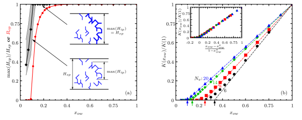
Figure 6: Network simulations: (a) Maximal height of the interconnected porosity (black line: median values - grey band: 1st and 99th percentile) and interconnected porosity (red line: mean values) as a function of the open walls fraction $x_{ow}$ for $N_{v}=14$, (b) Dimensioless permeability $K(x_{ow})/K(1)$ as a function of open walls fraction $x_{ow}$ for various neighbor bubbles number $N_{v}$ (arrows point to the abscissa $x_{ow}=x_{ow}^{\star}$), inset: same data with another abscissa $(x_{ow}-x_{ow}^{\star})/(1-x_{ow}^{\star})$.

Network simulations performed on different structures (Fig. 3) are helpful to study in details percolation effects for such foam structures and to calculate both the heights of interconnected pores $H_{ip}$ and the fraction of percolating porosity $R_{op}$ (Fig. 6a). In the case $N_{v}=14$, the maximal height of interconnected pores is equal in average to the sample height $H_{sp}$ for $x_{ow}>0.1$, and connected porosity percolates throughout the sample. Regarding the permeability (Fig. 6b), simulations performed with homogeneous local permeabilities show that the slope of the affine part of $K(x_{ow})$ depends on the number of neighbor bubbles $N_{v}$. The affine part of $K(x_{ow})$ intercepts the abscissa to a critical concentration given by $x_{ow}^{\star}=2/N_{v}$. Inset of Fig. 6b shows that the ratio $K\left(x_{ow}\right)/K\left(1\right)$ in porous material having homogeneous local permeability is linearly dependent on a single parameter $(x_{ow}-x_{ow}^{\star})/(1-x_{ow}^{\star})$ except in the vicinity of percolation.

A deeper analysis of results shows that percolation occurs on average when $x_{ow}$ is in the range $\left[0.55x_{ow}^{\star};0.65x_{ow}^{\star}\right]$, and that the fraction of open walls within the percolating porosity $x_{ow}^{\prime}$ is larger than the global value $x_{ow}$. As shown in Fig. 7, the relative gap between both fractions of open walls is exponentially dependent on the reduced fraction $(x_{ow}-x_{ow}^{\star})/(1-x_{ow}^{\star})$. The fraction $x_{ow}^{\prime}$ and the fraction of percolating porosity $R_{op}$ can be approximated by the following equations:

$$\frac{x_{ow}^{\prime}}{x_{ow}}=1+\beta\exp\left(-\alpha\frac{x_{ow}-x_{ow}^{\star}}{1-x_{ow}^{\star}}\right)$$ (4)

$$R_{op}=1-\min\left(1,\exp\left(-1.25-\alpha\frac{x_{ow}-x_{ow}^{\star}}{1-x_{ow}^{\star}}\right)\right)$$ (5)

with $\alpha=2.56\left(\frac{N_{v}}{2}-1\right)+3$ and $\beta=0.123\left(\frac{N_{v}}{2}-1\right)^{0.23}$

From a practical point of view, these previous formulas might be useful to estimate the percolating porosity and the open walls fraction inside the percolating porosity by measuring for a real foam, the fraction of open walls and the number of neighbor pores.

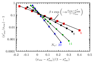
Figure 7: Excess fraction of open walls within the percolating porosity as a function of the reduced fraction of open walls for various neighbor numbers $N_{v}$.

III Effective medium model for permeability

III.1 Description

In this section, we present an effective permeability model of pores network connected by local permeabilities ${k_{i}}$. This model is based on a self-consistent calculation of the mean local permeability and a calculation of the macroscopic permeability. Details leading to Eqs. 6-7 are given in Appendix.

The mean local permeability $\bar{k}$ is calculated iteratively from (Kirkpatrick, 1973; Adler, 1992):

$$\frac{1}{\overline{k}+n\overline{k}}=\sum_{i}\frac{x_{i}}{k_{i}+n\overline{k}}$$ (6)

with $x_{i}$ the fraction of local permeability $k_{i}$ and $n=\frac{N_{v}}{2}-1$.

In a few simple cases, this equation possesses analytical solutions (e.g. binary mixture of local permeabilities, see Appendix).

The macroscopic effective permeability is then deduced from the mean local permeability $\bar{k}$,

$$K\approx\frac{n}{2}\overline{k}$$ (7)

In the next section, the present model is referred as EM model.

III.2 Comparison between network simulations and EM model predictions

In this part, we compare the predictions of EM model to the network simulations. We consider successively three cases: (i) mixing of two local permeabilities in a fully open material, (ii) mixing of closed and open walls characterized by a single local permeability, (iii) mixing of closed walls and two local permeabilities.

(i) As shown in Fig. 8, EM model predictions are in good agreement with the network calculation results for various ratios $k_{1}/k_{2}$.

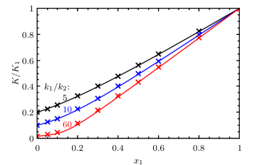
Figure 8: Comparison of self-consistent model predictions (full line) to network simulations (cross) with $N_{v}=14$.

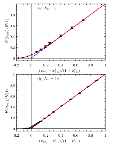
Figure 9: Comparison between EM model and network simulations (black diamond) for various neighbor pores numbers. “EM0” (dashed blue line) is based on the global open walls fraction (Eq. (8)), and “EM1” (red line) is based on the open walls fraction within the percolating porosity (Eq. (9)).

(ii) Mixing closed walls with identicaly open walls is a peculiar case of the latter configuration: the local permeability associated to the close walls is equal to zero. In this case, Eqs. 6 and 7 have an analytical solution leading to:

$$\frac{K}{K_{1}}=\frac{x_{1}-x_{ow}^{\star}}{1-x_{ow}^{\star}}$$ (8)

As shown in Fig. 9, this solution “EM0” reproduces correctly the linear relationship between the permeability and the parameter $(x_{ow}-x_{ow}^{\star})/(1-x_{ow}^{\star})$. However, the permeability evolution is not accurately reproduced in the vicinity of the percolation threshold. This discrepancy can be significantly reduced if the fraction of open walls inside the percolating porosity is used instead of the global open walls fraction (“EM1” in fig.9), leading to the following equation:

$$\frac{K}{K_{1}}=\frac{x_{1}^{\prime}-x_{ow}^{\star}}{1-x_{ow}^{\star}}R_{op}$$ (9)

The fraction of open walls inside the percolating porosity can be estimated from the global open walls fraction by using Eq. 4.

For generalization purpose, one can write:

$$\frac{1}{\overline{k^{\prime}}+n\overline{k^{\prime}}}=\sum_{i}\frac{x_{i}^{\prime}}{k_{i}+n\overline{k^{\prime}}}$$ (10)

$$K\approx R_{op}\frac{n}{2}\overline{k^{\prime}}$$ (11)

where $x_{i}^{\prime}$ is the fraction of walls inside the percolating porosity having a local permeability equal to $k_{i}$.

After Eq.9, the physical meaning of the critical concentration $x_{ow}^{\star}=2/N_{v}$ is now clarify: at least two open walls per bubble located in the percolating porosity are required to start a sufficient interconnection of pores.

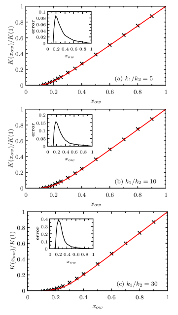
Figure 10: Comparison of “EM1” model predictions (red line) to network simulations (black cross) with $N_{v}=14$. Insets are the relative error of the EM model prediction.

(iii) This configuration corresponds to the latter case but with two local permeabilities having the same fraction $x_{1}=x_{2}$, so that Eqs. 10 and 11 can be used. Comparison with pore-network simulations is shown in Fig. 10 for various ratios of local permeabilities $k_{2}/k_{1}$ with $N_{v}=14$. As already mentionned, EM model reproduces correctly results from pore-network simulations (fig. 5). However, for low ratio $k_{2}/k_{1}$, deviations are observed in the vicinity of the percolation threshold.

IV Comparison with experiments

In the next section, we detail experiments conducted on real solid foams: foaming process, microstructural characterization, permeability measurements, etc. Finally, we compare experimental results with predictions of EM model.

IV.1 Elaboration of controlled polymer foams

We elaborate solid polymer foam samples having fixed values for both gas volume fraction and monodisperse bubble diameter $D_{b}$, but a tunable membrane content. The experimental procedure can be described as follows (see Fig. 11): (1) monodisperse precursor aqueous foam is generated. Foaming liquid, i.e. TTAB (TetradecylTrimethylAmonium Bromide) at 3 g/L in water, and nitrogen are pushed through a T-junction allowing the bubble size control by adjusting the flow rate of each fluid. Produced bubbles are collected in a glass column and a constant gas fraction over the foam column is set at 0.99 by imbibition from the top with foaming solution (Lorenceau et al., 2009). (2) An aqueous gelatin solution is prepared at a mass concentration $C_{gel}$ within the range 12-18%. The temperature of this solution is maintained at $T$ $\approx$ 60°C in order to remain above the sol/gel transition ($T_{(s/g)}\approx$ 30°C). (3) The precursor foam and the hot gelatin solution are mixed in a continuous process thanks to a mixing device based on flow-focusing method (Khidas et al., 2015, 2014). By tuning the flow rates of both the foam and the solution during the mixing step, the gas volume fraction can be set, $\phi_{0}$ = 0.8. Note also that the bubble size is conserved during the mixing step. The resulting foamy gelatin is continuously poured into a cylindrical cell (diameter: 40 mm and height: 40 mm) which is rotating around its axis of symmetry at approximately 50 rpm. This process allows for gravity effects to be compensated until the temperature decreases below $T_{(s/g)}$. (4) The cell is let one hour at 5°C, then one week in a climatic chamber ($T$ = 20°C and RH = 30%). During this stage, water evaporates from the samples and the gas volume fraction increases significantly. (5) After unmolding, a slice (thickness: 20 mm and diameter: 40 mm) is cut.

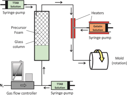
Figure 11: Foaming process

IV.2 Characterization of the foam samples

Pore volume fraction:

As the density of dried gelatin was measured to be 1.36, volume and weight measurements of the dried foam samples give the pore volume fraction. For the gelatin concentrations used in this study, the pore volume fraction is found to vary between 0.977 and 0.983, so that in the following we will consider that this parameter is approximately constant and equal to 0.980±0.003.

Pore size:

Through a preliminary calibration, observation of the sample surface (see Fig. 12a) allows for the pore (bubble) size to be measured. The calibration procedure can be described as follows: bubbles collected in the glass column (precursor in the Fig. 11) are sampled and squeezed between two glass plates separated from 100 µm. Then the surface exposed with a microscope is measured, and using volume conservation, bubble gas volume is determined and the mean bubble diameter $D_{b}$ is obtained with a precision better than 3%. Moreover, we measure the mean length $L_{p}$ that characterized the Plateau borders of the precursor foam at the column wall. We obtain the following relationship, $D_{b}=(1.68\pm 0.06)L_{p}$, that can be used afterwards for measuring the pore size in the dried gelatin samples. We measure $D_{b}$ = 810 µm (the absolute error on $D_{b}$ is ± 30 µm) for all the samples.

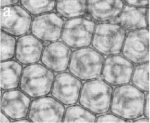
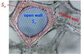
Figure 12: Characterization of foam samples

Cell wall characteristics:

We characterize cell walls in our samples through observation with a microscope on both top and bottom sample surfaces (see Fig. 12). For each sample, a large number of cell walls, $N_{w}$¿100, were observed in order to determine the following parameters: the number of open walls, $N_{ow}$, and the proportion of open walls:

$$x_{ow}=N_{ow}/N_{w}$$ (12)

The proportion of closed walls is therefore $x_{cl}=1-x_{ow}$ . Note that those open walls exhibit various aperture sizes, so the aperture ratio of walls is measured:

$$\delta_{ow}^{\prime\prime}=(S_{o}\text{\textfractionsolidus}S_{w})^{1/2}$$ (13)

where $S_{o}$ is the aperture area and $S_{w}$ is the total area of the window (see Fig. 12).

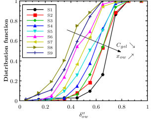
Figure 13: Distribution function of aperture factors $\delta_{ow}^{\prime\prime}$

The structural characterization is completed by a measurement of the membrane thickness through SEM images. From nine micrographs the average thickness has been measured to be equal to 1.5±0.25 µm, which is close to thicknesses measured for similar polymer foams (Yasunaga et al., 1996; Hoang et al., 2014; Gao et al., 2016).

Fig. 13 shows the distribution function of aperture factor for the samples, and Table 1 gives their corresponding mean value $<\delta_{ow}^{\prime\prime}>$ and their proportion of open walls $x_{ow}$.

Table 1: Characteristics of foam samples

Sample		S1	S2	S3	S4	S5	S6	S7	S8	S9
$C_{gel}$ (%)		12	13	16	16	16	17	18	18	18
$<\delta_{ow}^{\prime\prime}>$		0.72	0.68	0.67	0.62	0.59	0.50	0.54	0.42	0.46
$x_{ow}$		0.93	0.83	0.79	0.69	0.60	0.54	0.32	0.22	0.15
$10^{3}*K/D_{b}^{2}$	direct meas.	17.63	9.10	6.99	3.83	out of range
	acoustic meas.	16.89	8.02	7.58	2.79	2.33	1.43	0.579	0.140	0.017

IV.3 Foam permeability

Permeability measurement:

We determined the permeability by acoustic measurements performed in a three-microphone impedance tube (Utsuno et al., 1989; Salissou and Panneton, 2010). Permeability value is deduced from the imaginary part of the low frequency behavior of the effective density (Panneton and Olny, 2006): $K=-\mu/\lim_{\omega\to 0}[\Im(\omega\rho)]$. Note that the diameter of the samples is slightly larger than 40 mm so that air leakage issue and sample vibration were successfully avoided. The air permeability is determined on frequencies ranging from 200 Hz to 400 Hz.

Samples showing high permeability, i.e. $K>10^{-9}m^{2}$, were characterized by a direct measurement of the pressure drop $\Delta P_{sp}$ as a function of air flow rate $Q$ within steady laminar conditions, and the Darcy permeability was determined as follows(standard, ):

$$K=\mu QH/A\Delta P_{sp}$$ (14)

with the thickness of sample $H$$\approx$ 20 mm and the circular cross-sectional area $A$$\approx$1.25 $cm^{2}$.

Comparison to theoretical predictions:

Theoretical calculations are performed by assuming the Sampson local permeability ($k_{i}=d_{i}^{3}/24D_{b}$) in Eq. 10 and by using Eq. 11. The size of aperture $d_{i}$ is calculated from the aperture factor $\delta_{ow}^{\prime\prime}$ and the mean size of bubbles $D_{b}$:

$$d_{i}=\delta_{ow}^{\prime\prime}\left\langle t_{w}/D_{b}\right\rangle D_{b}$$

The ratio $\left\langle t_{w}/D_{b}\right\rangle$ as well as the pore neighbor number are assumed to be given by Kelvin cell structure: $(\frac{8}{14}\sqrt{3}L+\frac{6}{14}L)/2\sqrt{2}L\approx 0.5$4 and $N_{v}=14$. Moreover, aperture distributions shown in Fig.13 allows to calculate the fraction $x_{i}$ of walls having an aperture size equal to $d_{i}$. Fig. 14 shows that the theoretical predictions are in good agreement with experimental measurements. Various reasons can be mentioned to explain the discrepancy observed at high permeability: error caused by assuming the real foam structure like a Kelvin structure, error in measurement of aperture size (a theoritical calculation of permeability with walls apertures 30% greater is enough to delete the gap), error in permeability measurement due to air leak around the sample.

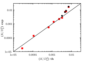
Figure 14: Comparison of direct (dot) and acoustical (square) measurements of foam permeability to theoretical predictions.

V Conclusion

We have studied the static permeability of solid foams by combining different approaches: (i) Numerical approach: FEM simulations computing Stokes problem both at the pore scale and at the macro-scale, a simulation of simplified flow performed on a network of interconnected pores interacting by Sampson local permeabilities, (ii) Theoretical approach: a model of effective permeability based on the same theoretical framework than network simulations has been developed, (iii) Experimental approach: controlled samples of gelatin foams have been prepared, dried and fully characterized (bubble size, wall aperture, air permeability). FEM simulations allowed us to validate the use of network simulations to predict the effects on permeability of both the wall aperture size and the amount of closed walls. Compared to FEM simulations, networks simulations are low computational cost and can be widely used to test the predictions of the EM model, and to study the percolation effect of the pore network. These different approaches made it possible to develop and validate a model of effective foam permeability (Eqs. 3, 4, 5, 10 and 11).

For future studies, network simulations could be useful to study permeability of various porous foamy materials (topologically disordered foams or containing double porosity,…) and to check the ability of EM model to predict permeability of such materials.

Appendix

Here, we detail the calculation of the mean local permeability. We consider a cross-section of foam (fig. 15a) and calculate the mean local permeability $\bar{k}$ of a foam containing different local permeabilities $\left\{k_{i}\right\}$. To represent a pore inside the cross-section, we consider a half pore connected to $N_{v}/2$ effective pores such as $n=\frac{N_{v}}{2}-1$ membranes have a local permeability equal to the mean local permeability $\bar{k}$ and the last one located at the $p^{th}$ position has a permeability equal to $k_{i}$ (fig. 15b). Due to the heterogeneity induced by the local permeability $k_{i}$, the pressure inside the central pore $P_{i,p}$ is different from the mean pressure $\bar{P}$. Pressures inside neighbor effective pores are supposed equal to the effective pressure expected for each peculiar position of the neighbor pore: $\bar{P}+\alpha_{r}\Delta\bar{P}$ with $\alpha_{r}=z_{r}/D_{b}$. The total flow rate passing through the central half pore is equal to:

$q_{i,p}=\frac{D_{b}}{\mu}\sum_{r=1}^{n+1}q_{r}=\frac{D_{b}}{\mu}\sum_{r=1}^{n+1}k_{r}\left(\bar{P}+\alpha_{r}\Delta\bar{P}-P_{i,p}\right)$

where $k_{r}=\bar{k}$ for $r\neq p$, and $k_{i}$ for $r=p$.

The total flow rate can be written in a more useful way as:

$q_{i,p}=\frac{D_{b}}{\mu}\left[\sum_{r=1}^{n+1}\bar{k}\left(\bar{P}-P_{i,p}+\alpha_{r}\Delta\bar{P}\right)+\left(k_{i}-\bar{k}\right)\left(\bar{P}-P_{i,p}+\alpha_{p}\Delta\bar{P}\right)\right]$ .

The effective flow rate $\bar{q}$ passing through the effective pore is obtained by considering $k_{i}=\bar{k}$ and $P_{i,p}=\bar{P}$ in the previous equation:

$\bar{q}=\frac{D_{b}}{\mu}\sum_{r=1}^{n+1}\bar{k}\alpha_{r}\Delta\bar{P}$.

Therefore, the flow rate $q_{i,p}$ can be expressed in function of $\bar{q}$:

$q_{i,p}=\bar{q}+\frac{D_{b}}{\mu}\left[\left(n+1\right)\bar{k}\left(\bar{P}-P_{i,p}\right)+\left(k_{i}-\bar{k}\right)\left(\bar{P}-P_{i,p}+\alpha_{p}\Delta\bar{P}\right)\right]$.

In the following, we suppose that the total flow rate passing through the central half pore $q_{i,p}$ is equal to the effective flow rate $\bar{q}$ leading to:

$0=\left(n+1\right)\bar{k}\left(\bar{P}-P_{i,p}\right)+\left(k_{i}-\bar{k}\right)\left(\bar{P}-P_{i,p}+\alpha_{p}\Delta\bar{P}\right)$.

This hypothesis leads to the pressure inside the central pore:

$$P_{i,p}=\bar{P}+\frac{\left(k_{i}-\bar{k}\right)}{n\bar{k}+k_{i}}\alpha_{p}\Delta\bar{P}$$

Now, we may impose the self-consistency condition, requiring that the average $\left\langle P_{i,p}\right\rangle_{p,i}=\left\langle\left\langle P_{i,p}\right\rangle_{p}\right\rangle_{i}$ is equal to the effective pressure $\bar{P}$ leading to:

$$\left\langle\frac{k_{i}-\bar{k}}{n\bar{k}+k_{i}}\right\rangle_{i}\left\langle\alpha_{p}\right\rangle_{p}\Delta\bar{P}=0$$

The previous equation can be rewritten in an alternative form:

$$\left\langle\frac{1}{n\bar{k}+k_{i}}\right\rangle_{i}=\frac{1}{\left(n+1\right)\bar{k}}$$

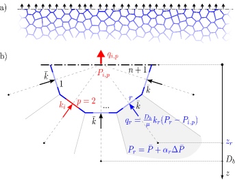
Figure 15: (a) Cross-section of foam, (b) Geometry of a half pore representative of pores contained inside the foam cross-section. Note that we have to consider $n+1$ configurations for the position $p$ of the membrane associated with the permeability $k_{i}$. Figure depicts the case $p=2.$

To determine the macroscopic effective permeability, we calculate the macroscopic flow rate $Q$ passing through the whole cross-section $A$ containing $N_{w}$ walls having a local permeability equal to $\bar{k}.$ Moreover, we suppose that the effective gradient of pressure around the cross-section $\frac{\Delta\bar{P}}{D_{b}}$ is equal to the mean pressure gradient $\frac{\Delta P_{sp}}{H}$. Then the macroscopic flow rate is given by:

$$Q=\frac{D_{b}}{\mu}\left[\sum_{w=1}^{N_{w}}\alpha_{w}\right]\bar{k}\Delta\bar{P}=\frac{D_{b}}{\mu}*N_{w}\left\langle\alpha\right\rangle_{p}*\bar{k}*\frac{\Delta P_{sp}}{H}D_{b}$$

leading to the macroscopic effective permeability:

$$K=\frac{N_{w}}{A}\left\langle\alpha\right\rangle_{p}D_{b}^{2}\bar{k}$$

In considering the continuous limit for the calculation of $\left\langle\alpha\right\rangle_{p}$, we obtain: $\left\langle\alpha\right\rangle_{p}=\frac{1}{2\pi}\int_{0}^{2\pi}\int_{0}^{\pi/2}sin(\theta)cos(\theta)d\theta d\varphi=\frac{1}{2}$. And in the case of a Kelvin structure, the surface wall density $N_{w}/A$ is equal to $n/D_{b}^{2}$.

In the case of a binary mixture of local permeabilities (e.g. fully open foam), the mean local permeability $\bar{k}$ is given by the following equation:

$\frac{\bar{k}}{k_{\infty}}=\frac{1}{2}\left[\alpha+\left(\alpha^{2}+4\left(1-\alpha\right)\frac{k_{0}}{k_{\infty}}\right)^{0.5}\right]$

with

$\alpha=1-\frac{k_{1}k_{2}}{nk_{0}k_{\infty}}$

$k_{\infty}=k_{Voigt}=x_{1}k_{1}+x_{2}k_{2}$

$k_{0}=k_{Reuss}=\left(\frac{x_{1}}{k_{1}}+\frac{x_{2}}{k_{2}}\right)^{-1}$

$k_{\infty}$ and $k_{0}$ correspond respectively to the permeability of an infinitely interconnected network ($N_{v}\rightarrow\infty$) and this one of a poorly interconnected network ($N_{v}=2$).

References

- [1] Standard test method for airflow resistance of acoustical materials,(astm c 522-80, 1980)
- Adler [1992] P.M. Adler. Porous media : geometry and transports. Chap. 3. Butterworth/Heinemann, 1992.
- Allard and Atalla [2009] J. F. Allard and N. Atalla. Propagation of sound in porous media: Modelling sound absorbing materials. John Wiley & Sons, 2009.
- Cantat et al. [2013] I. Cantat, S. Cohen-Addad, F. Elias, F. Graner, R. Höhler, O. Pitois, F. Rouyer, and A. Saint-Jalmes. Foams: structure and dynamics. Oxford University Press, 2013.
- Doutres et al. [2013] O. Doutres, N. Atalla, and K. Dong. A semi-phenomenological model to predict the acoustic behavior of fully and partially reticulated polyurethane foams. Journal of Applied Physics, 113:054901, 2013.
- Fatt [1956] I. Fatt. The network model of porous media. Petroleum Transactions, AIME, 207:141–181, 1956.
- Gao et al. [2016] K. Gao, J. van Dommelen, and M. Geers. Microstructure characterization and homogenization of acoustic polyurethane foams: Measurements and simulations. International Journal of Solids and Structures, 100-101:536–546, 2016.
- Hoang and Perrot [2012] M. T. Hoang and C. Perrot. Solid films and transports in cellular foams. Journal of Applied Physics, 112:054911, 2012.
- Hoang et al. [2014] M.T. Hoang, G. Bonnet, H. Tuan Luu, and C. Perrot. Linear elastic properties derivation from microstructures representative of transport parameters. J Acoust Soc Am., 135:3172–3185, 2014.
- Idel’Cik [1996] I.E. Idel’Cik. Hanbook of hydraulic resistance. Begell House Inc., 1996.
- Jivkov et al. [2013] A. P. Jivkov, C. Hollis, F. Etiese, S. A. McDonald, and P. J. Withers. A novel architecture for pore network modelling with applications to permeability of porous media. Journal of Hydrology, 486:246–258, 2013.
- Johnson et al. [1987] D. L. Johnson, J. Koplik, and R. Dashen. Theory of dynamic permeability and tortuosity in fluid-saturated porous media. J. Fluid Mech., 176:379–402, 1987.
- Khidas et al. [2014] Y. Khidas, B. Haffner, and O. Pitois. Capture-induced transition in foamy suspensions. Soft Matter., 10:4137–4141, 2014.
- Khidas et al. [2015] Y. Khidas, B. Haffner, and O. Pitois. Critical size effect of particles reinforcing foamed composite materials. Composites Science and Technology, 119:62–67, 2015.
- Kirkpatrick [1973] S. Kirkpatrick. Percolation and conduction. Rev. Mod. Phys., 45:574–588, 1973.
- Kumar and Topin [2017] Prashant Kumar and Frédéric Topin. Predicting pressure drop in open-cell foams by adopting forchheimer number. International Journal of Multiphase Flow, 94:123–136, 2017.
- Lorenceau et al. [2009] E. Lorenceau, N. Louvet, F. Rouyer, and O. Pitois. Permeability of aqueous foams. European Physical Journal E., 28, 2009.
- [18] C. Lusso and X. Chateau. Disordered monodisperse 3d open-cell foams: Elasticity, thermal conductivity and permeability.
- Marcke et al. [2010] P. Van Marcke, B. Verleye, J. Carmeliet, D. Roose, and R. Swennen. An improved pore network model for the computation of the saturated permeability of porous rock. Transport in Porous Media, 85:451–476, 2010.
- Mavko and Nur [1997] G. Mavko and A. Nur. The effect of a percolation threshold in the kozeny-carman relation. Geophysics, 62:1480–1482, 1997.
- Panneton and Olny [2006] R. Panneton and X. Olny. Acoustical determination of the parameters governing viscous dissipation in porous media. J. Acoust. Soc. Am., 119:2027–2040, 2006.
- Perrot et al. [2007] C. Perrot, R. Panneton, and X. Olny. Periodic unit cell reconstruction of porous media: Application to open-cell aluminum foams. Journal of Applied Physics, 101:113538, 2007.
- Salissou and Panneton [2010] Y. Salissou and R. Panneton. Wideband characterization of the complex wave number and characteristic impedance of sound absorbers. J. Acoust. Soc. Am., 128:2868–2876, 2010.
- Sampson [1891] R. A. Sampson. On stokes’s current function. Philosophical Transactions of the Royal Society of London. A, 182:449–518, 1891.
- Utsuno et al. [1989] H. Utsuno, T. Tanaka, T. Fujikawa, and A. F. Seybert. Transfer function method for measuring characteristic impedance and propagation constant of porous materials. J. Acoust. Soc. Am., 86:637–643, 1989.
- van Melick and Geurts [2013] P. A. J. van Melick and B. J. Geurts. Flow through a cylindrical pipe with a periodic array of fractal orifices. Fluid Dynamics Research, 45:061405, 2013.
- Vogel [2000] H. J. Vogel. A numerical experiment on pore size, pore connectivity, water retention, permeability, and solute transport using network models. European Journal of Soil Science, 51:99–105, 2000.
- Xiong et al. [2015] Q. Xiong, C. Joseph, K. Schmeide, and A. P. Jivkov. Measurement and modelling of reactive transport in geological barriers for nuclear waste containment. Phys. Chem. Chem. Phys., 17:30577–30589, 2015.
- Xiong et al. [2016] Q. Xiong, T. G. Baychev, and A. P. Jivkov. Review of pore network modelling of porous media: Experimental characterisations, network constructions and applications to reactive transport. Journal of Contaminant Hydrology, 192:101–117, 2016.
- Yasunaga et al. [1996] K. Yasunaga, R. Neff, X. Zhang, and C. Macosko. Study of cell opening in flexible polyurethane foam. Journal of cellular plastics, 32:427–448, 1996.