INCT, Universidad De Atacama, calle Copayapu 485, Copiapó, Atacama, Chile
Department of Physics, University of Oxford, Oxford, UK
LESIA, Observatoire de Paris, PSL Research University, CNRS, Sorbonne Universités, UPMC Univ. Paris 06, Univ. Paris Diderot, Sorbonne Paris Cité, 5 Place Jules Janssen, 92195 Meudon, France
Virtual Planetary Laboratory, University of Washington, Seattle, WA 98125, USA
Univ. Grenoble Alpes, IPAG; CNRS, IPAG, 38000 Grenoble, France
Univ. Lyon, Univ. Lyon 1, ENS de Lyon, CNRS, CRAL UMR 5574, 69230 Saint-Genis-Laval, France
Aix-Marseille Université, CNRS, LAM – Laboratoire d’Astrophysique de Marseille, UMR 7326, 13388 Marseille, France
Nucleo de Astronomía, Facultad de Ingeniería, Universidad Diego Portales, Av. Ejercito 441, Santiago, Chile
Universidad de Chile, Camino el Observatorio, 1515 Santiago, Chile
Max-Planck-Institut für Astronomie, Känigstuhl 17, 69117 Heidelberg, Germany
Department of Astronomy, Stockholm University, SE-10691 Stockholm, Sweden
INAF – Osservatorio Astrofisico di Arcetri, Largo E. Fermi 5, I-50125, Firenze, Italy
INAF – Osservatorio Astrofisico di Catania, Via S. Sofia 78, I-95123, Catania, Italy
INAF – Osservatorio Astronomico di Capodimonte, Via Moiariello 16, I-80131 Napoli, Italy
Unidad Mixta Internacional Franco-Chilena de Astronomía, CNRS/INSU UMI 3386 and Departamento de Astronomía, Universidad de Chile, Casilla 36-D, Santiago, Chile
INAF Osservatorio Astronomico di Brera, via Emilio Bianchi 46, 23807, Merate (LC), ITALY
INAF – Istituto di Astrofisica Spaziale e Fisica Cosmica di Milano, Via E. Bassini 15, I-20133 Milano, Italy
Universite Cote d’Azur, OCA, CNRS, Lagrange, France
New spectro-photometric characterization of the substellar object HR 2562 B using SPHERE††thanks: Based on observations made with European Southern Observatory (ESO) telescopes at Paranal Observatory in Chile, under programma ID 198.C-0209(D).
Abstract
Aims. HR 2562 is an F5V star located at 33 pc from the Sun hosting a substellar companion that was discovered using the GPI instrument. The main objective of the present paper is to provide an extensive characterisation of the substellar companion, by deriving its fundamental properties.
Methods. We observed HR 2562 with the near-infrared branch (IFS and IRDIS) of SPHERE at the VLT. During our observations IFS was operating in the band, while IRDIS was observing with the broad-band filter. The data were reduced with the dedicated SPHERE GTO pipeline, which is custom-designed for this instrument. On the reduced images, we then applied the post-processing procedures that are specifically prepared to subtract the speckle noise.
Results. The companion is clearly detected in both IRDIS and IFS datasets. We obtained photometry in three different spectral bands. The comparison with template spectra allowed us to derive a spectral type of T2-T3 for the companion. Using both evolutionary and atmospheric models we inferred the main physical parameters of the companion obtaining a mass of MJup, = K and =.
Conclusions.
Key Words.:
Instrumentation: spectrographs - Methods: data analysis - Techniques: imaging spectroscopy - Stars: planetary systems, HR25621 Introduction
In the last decade, the research field focussed on the atmospheric characterization of bound sub-stellar objects (i.e., brown dwarfs and giant planets) has experienced an outstanding boost. In fact, high-contrast imaging observations have granted the discovery of an increasing number of substellar companions (Chauvin et al. 2004, 2005; Marois et al. 2008; Lagrange et al. 2010; Biller et al. 2010; Rameau et al. 2013; Bailey et al. 2014; Macintosh et al. 2015; Gauza et al. 2015; Milli et al. 2017; Bowler et al. 2017) . In particular, the new generation of extreme adaptive optics (XAO) high-contrast imaging facilities such as e.g., SPHERE at VLT (Beuzit et al. 2008) and GPI at Gemini (Macintosh et al. 2014) have proven to be remarkably efficient for this purpose. Several recent examples of spectroscopic characterization of substellar companions with those instruments include HD 95086 b (De Rosa et al. 2016), 51 Eri b (Macintosh et al. 2015; Samland et al. 2017), Pic b (Chilcote et al. 2017), HD 1160 B (Maire et al. 2016; Garcia et al. 2017), HD 984 B (Johnson-Groh et al. 2017), GJ 504 b (Bonnefoy 2015), GJ 758 B (Vigan et al. 2016), the four planets of the HR 8799 system (Bonnefoy et al. 2016; Zurlo et al. 2016) and HR 3549 B (Mesa et al. 2016).
HR 2562 (HIP 32775; HD 50571) is an F5V star with an estimated mass of M1.3 M⊙ and a distance of d=33.630.48 pc (see Section 2). Moór et al. (2006) identified a debris disk around it by exploiting IRAS and Spitzer data. Chen et al. (2014) modeled the stellar spectral energy distribution (SED) with a two-components disk placed at 1.1 and 341.6 au respectively. More recently, Moór et al. (2015), using Herschel data, derived a dust radius of 112.18.4 au with evidence for an inner hole with a radius between 18 and 70 au, and an high inclination of . Konopacky et al. (2016) found a substellar companion with mass in the brown dwarf regime of MJup and effective temperature = K. Its separation of 0.6′′ corresponding to 20 au from the star put it into the hole in the disk and its separation and position angle are compatible with its orbit being coplanar with the disk itself.
HR 2562 was observed with SPHERE in order to gather a thorough investigation of the spectral properties of its substellar companion, constraining the physical parameters and fundamental properties, and to obtain new high-precision astrometric data to better define its orbit and the relation with the disk. In this paper we discuss the spectro-photometric data obtained for this target, whereas the astrometric data will be discussed in a second paper (Maire et al., in prep.).
2 Host star properties
A careful determination of the fundamental parameters of the host star is crucial as to obtain reliable and robust estimates of the substellar companion properties. In particular, the most crucial issue is the stellar age that is poorly defined for HR 2562, as for mid F-type stars in general. Asiain et al. (1999) defined an age of 300120 Myr classifying HR 2562 as a member of the B3 group. A similar age of 300 Myr was subsequently determined by Rhee et al. (2007) using space motions, lithium non-detection and X-ray luminosity. Exploiting the metallicity and the temperature from the Geneva-Copenaghen survey, Casagrande et al. (2011) defined a much older age of 0.9-1.6 Gyr and a similar result of 0.9 Gyr was found by Pace (2013) according to the chromospheric activity. Finally, Moór et al. (2011) derived an age range of Myr using evolutionary models. We tried to determine the main stellar parameters following the methods described in Desidera et al. (2015) but more specifically tuned for a mid-F star as previously done for HD 206893 B in Delorme et al. (2017).
2.1 Spectroscopic parameters
In order to carry out a spectroscopic analysis of HR 2562 (aiming at deriving radial and rotational velocities, along with atmospheric parameters, , log, and metallicity [Fe/H]), we retrieved from ESO archive two UVES spectra111Prog. ID 096.C-0238(A), acquired on the same night, and two FEROS spectra222Prog. ID 094.A-9012(A), separated by a few months. In all cases, data reduction was performed using the on-line pipeline tools provided by ESO.
From these spectra we have measured the radial velocity (RV) and the projected rotation velocities (v), as listed in Table 1, using a custom cross-correlation function (CCF) procedure. While our radial and projected rotational velocity estimates agree fairly well with each other, there is a significant discrepancy (about 6 km/s in RV and about 25 km/s in v sin) with the results obtained with CORAVEL333These differences can be explained if the star is an SB2 system with the components seen at similar velocities at the epoch of FEROS and UVES observations. However, this hypothesis has several difficulties. There are no significant RV differences between the FEROS and UVES epochs and the two CORAVEL observations, suggesting a moderately long period but the period should be short enough to ensure a RV amplitude large enough to explain the v variations. Also, the acquisition images obtained with SPHERE does not show the presence of equal luminosity companions down to separation of about 40 mas. Therefore, the projected separation at the epoch of the SPHERE observations would have been smaller than about 1.35 au. All these constraints can be satisfied only by a very narrow range of binary parameters. Furthermore, for an SB2 system with similar components (as required to explain a variable FWHM of the CCF) an unphysical position on color-magnitude diagram below main sequence is obtained. We then conclude that additional observations are needed to settle the issue of the binarity of the central star. (Andersen et al. 1985; de Medeiros & Mayor 1999; Nordström et al. 2004).
| Date | RV (km/s) | v sini (km/s) | Instrument | Reference |
|---|---|---|---|---|
| 2008-06-14 | 22.900.81 | 60.0 | CORAVEL | Andersen et al. (1985); Nordström et al. (2004) |
| 2009-05-29 | 21.580.80 | 60.0 | CORAVEL | Andersen et al. (1985); Nordström et al. (2004) |
| 2016-02-23 | 29.280.40 | 31.3 | UVES | this paper |
| 2016-03-26 | 27.720.43 | 35.0 | FEROS | this paper |
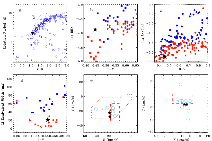
We confirm, in agreement with Asiain et al. (1999), that the kinematic parameters of the star are similar to those of the B3 group when adopting the Andersen et al. (1985) RV while they deviate significantly when adopting our own RV determination. Concerning the younger groups, no significant membership probability is returned using the on-line BANYAN II tool (Gagné et al. 2014) for both values of system RV. Taking the uncertainties in system RV into account, we do not consider the kinematic as constraining the stellar age in the following.
| Parameter | Value | Ref |
| V (mag) | 6.11 | Hipparcos |
| BV (mag) | 0.457 | Hipparcos |
| VI (mag) | 0.53 | Hipparcos |
| J (mag) | 5.3050.020 | 2MASS |
| H (mag) | 5.1280.029 | 2MASS |
| K (mag) | 5.0200.016 | 2MASS |
| Parallax (mas) | 29.730.40 | GaiaDR1 |
| (mas yr-1) | 4.8720.040 | GaiaDR1 |
| (mas yr-1) | 108.5680.040 | GaiaDR1 |
| RV (km s-1) | 27.720.43 | this paper |
| (K) | 659781 | Casagrande et al. (2011) |
| 4.30.2 | this paper | |
| 0.100.06 | this paper | |
| EW Li (mÅ) | 215 | this paper |
| A(Li) | 2.550.20 | this paper |
| (km s-1) | 33.22.6 | this paper |
| -5.210.06 | this paper | |
| Age (Myr) | 200-750 | this paper |
| 1.3680.018 | this paper | |
| 1.3340.027 | this paper |
The star was also detected by ROSAT, yielding . This value is within the locus of Hyades stars (Fig. 1, panel c). The chromospheric emission parameter obtained by Gray et al. (2006) (Fig. 1, panel b) is likely overestimated (see Desidera et al. 2015) and cannot give any constraint on the stellar parameters.
The highest-quality FEROS spectrum (median SNR=305 per pixel) was also used to derive the stellar parameters. The moderately fast rotation makes it challenging to perform a standard abundance analysis. Selecting 14 FeI and 2 Fe II isolated lines we derived =6650100 K, =4.30.2, [Fe/H]=+0.130.02 with internal error due to line-by-line scatter, and microturbulence =1.8 km/s. The same value of temperature is obtained by fitting the wings of the line, employing the SME code (Valenti & Piskunov 1996). The mild metal overabundance is also supported by Strömgren photometry (Casagrande et al. 2011) with [Fe/H]=+0.07. The effective temperature derived in that study is 659781 K. Considering the uncertainties in the spectral analysis for such a moderately fast-rotator mid F star, we adopt this latter value. Repeating the abundance analysis for the adopted yields [Fe/H]=+0.100.02.
Isochrone stellar age and stellar mass were derived exploiting the Bressan et al. (2012) stellar models and the PARAM interface (da Silva et al. 2006) with the input parameters above. The stellar age is not well constrained (630540 Myr), as expected for a star that lies close to the zero age main sequence (ZAMS). HR 2562 is not known as a variable star and Hipparcos photometry shows a scatter of only 0.007 mag from 118 photometric measurements along the mission lifetime. Therefore, it is unlikely that variability affects in significant way the isochrone ages.
2.2 Lithium abundance
The FEROS spectrum was also exploited to measure the lithium content, a key age indicator for mid-F stars thanks to the presence of the Li feature (Boesgaard & Tripicco 1986). Indeed a marked drop in Lithium abundance is seen for stars in a narrow range around 6660 K. The Lithium dip is clearly observed in the Hyades and other older open clusters (Balachandran 1995); it starts to be present at the age of the open cluster M35 (Steinhauer & Deliyannis 2004a) but it is not seen in the Pleiades and for younger clusters (Boesgaard et al. 1988). We performed the first measurement of lithium content in HR 2562, obtaining EW Li = 215 and, through spectral synthesis as described in Desidera et al. (2011); D’Orazi et al. (2017), A(Li) = 2.550.2. As for HIP 107412 that has similar (Delorme et al., in press), lithium provides the tightest constraints to the stellar age. Comparison with lithium observed in other intermediate age clusters and associations indicates that the Lithium content of HR 2562 is close to the upper boundaries of the locus of the Hyades, close to the lower boundaries of that of M35 (Steinhauer & Deliyannis 2004b) and well below the locus of the Pleiades (see Fig. 1, panel d). While the scatter in the Li-Teff relationship is significant for all the clusters, preventing a well-defined age calibration, this result confines the age of the star between 200 and 750 Myr. In the following we will consider these age limits in the derivation of the companion properties as well as 450 Myr as representative intermediate value. This age estimate is consistent (but more constraining) with the other dating techniques presented above and is slightly narrower than that adopted by Konopacky et al. (2016). The stellar mass and radius derived as above, altough allowing only this age range, (see Desidera et al. 2015) are 1.3680.018 and 1.3340.027 , respectively.
3 Observations and data reduction
HR 2562 was observed with SPHERE on February 6 2017, using a non-standard configuration for the IRDIFS mode. In this case, IFS (Claudi et al. 2008) was operating in the Y and J bands between 0.95 and 1.35 m while IRDIS (Dohlen et al. 2008) was using the H broad-band filter configuration instead of the standard dual band configuration in H2-H3 filters (Vigan et al. 2010). This choice was done with the aim to image the disk. The IFS data were composed by 16 datacubes of 5 frames with an exposure time of 64 s; those of IRDIS were composed by 16 datacubes of 20 frames with an exposure time of 16 s. The IRDIS observations were performed using a dithering pattern while no dithering was used for IFS. To be able to use the angular differential imaging (ADI; Marois et al. 2006a) technique, the field of view (FOV) was allowed to rotate during the observations, with the pupil fixed with respect to the detector. To maximize the total rotation of the FOV, we observed the star during its passage to the meridian with a total rotation of. For both IFS and IRDIS we acquired observing frames with the star image off-centered with respect to the coronagraph, to be able to calibrate the companion flux. In order to avoid saturation, a neutral density filter was employed. Moreover, we took frames with four satellite spots that are symmetrically located with respect to the central star by a suitable modification of the wavefront provided by the AO. This is done to properly determine the center of each frame: the use of satellite spots was first proposed by Sivaramakrishnan & Oppenheimer (2006) and Marois et al. (2006b) We refer to Langlois et al. 2013 and Mesa et al. 2015 for an extended discussion of their use within the SPHERE framework.
Both IFS and IRDIS data were reduced using the SPHERE data center 444http://sphere.osug.fr/spip.php?rubrique16&lang=en applying the appropriate calibrations following the SPHERE data reduction and handling (DRH, Pavlov et al. 2008) pipeline. More specifically, IRDIS dataset requires the application of dark and flat-field frames and the definition of the star center. On the other hand, for IFS observations the reduction steps include: dark and flat-filed correction, definition of the spectral positions, wavelength calibration, and the application of the instrumental flat. For IFS we then apply on the wavelength- calibrated datacubes (each of them composed by 39 monochromatic frames) the speckle subtraction exploiting the principal components analysis (PCA, Soummer et al. 2012) as described in Mesa et al. (2015) and Zurlo et al. (2014). For what concerns IRDIS we performed the speckle subtraction with both PCA and TLOCI (Marois et al. 2014), using the consortium pipeline (Galicher et al., in prep.).
4 Results
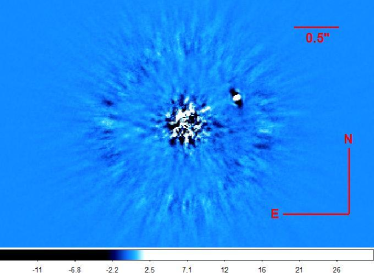
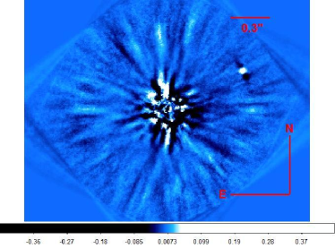
The data reduction procedure described in Sect. 3 provided the IFS and IRDIS final images displayed in Fig. 2. The companion is clearly detected with both instruments. However, it was not possible to image the debris disk, despite the fact we decided to employ the IRDIS H broad-band filter for this specific purpose. The companion was detected with a S/N of the order of 30 with IFS, and with a S/N of 20 with IRDIS. In both cases, we have exploited the PCA algorithm that allowed us to obtain the best results with respect to other algorithms.
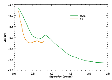
Moreover, we were able to define from the final images the contrast limit for IFS and IRDIS following the procedure devised in Mesa et al. (2015). The contrast values obtained was corrected to take into account the self-subtraction of the high-contrast imaging method. This was evaluated by injecting in the original datacube simulated planets of known flux. The resulting limiting contrast curves are displayed in Fig. 3 where we show that we could obtain a contrast better than at a separation of 0.3′′ or larger with IFS. As for IRDIS, we reach a contrast better than at separation larger than 1.5′′.
For the companion, we obtained photometric measurements for each spectral channel introducing a negative simulated planet in the original dataset at the companion position and running our PCA procedure. As a cross-check, we performed the same procedure using a classical ADI procedure and calculated the aperture photometry of the companion on the final images, after taking properly into account the self-subtraction. The three methods provide similar results and we list the final photometry obtained using the first method described above, for the Y, J and H bands (here and in all the following analysis we are using the 2MASS photometric system) in Tab. 3. The photometric errors on these values are mainly due to uncertainties on the attenuation factor of the method, to variations on the stellar PSF and of the stellar speckles noise during the observing sequence.
| 15.970.33 | 15.010.11 | 13.980.14 |
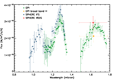
From the photometric data, we obtained a low resolution spectrum for the companion that was then converted from contrast to flux by multiplying it by a flux-calibrated BT-NEXTGEN (Allard et al. 2012) synthetic spectrum for the host star, adopting =6400 K, =4.0 and [M/H]=0.0 that gives the best fit with the SED of the star. The final result of this procedure is displayed in Fig. 4 and compared with the GPI spectrum from Konopacky et al. (2016). In the J-band, the SPHERE IFS and GPI spectra are very similar even if the peak at 1.27m is slightly higher (15% but however within the error bars - see Fig. 4) in the SPHERE IFS data. In the H band, in order to compare the IRDIS broad band result with GPI data, we integrated the GPI spectrum over the wavelength range of the IRDIS H broad band filter. In this case the IRDIS value is about 35% higher than that from GPI.
It is noteworthy, however, that systematic errors could be present between GPI and SPHERE probably due to differences in the algorithms for the spectral extraction and/or in the flux normalization procedure, as highlighted by Rajan et al. (2017) who compared the GPI (Macintosh et al. 2015) and SPHERE (Samland et al. 2017) results for 51 Eri b. For this reason, in the following analysis we will be using only the SPHERE data.
5 Discussion
5.1 Characterization of HR 2562 B
5.1.1 Color-magnitude diagram
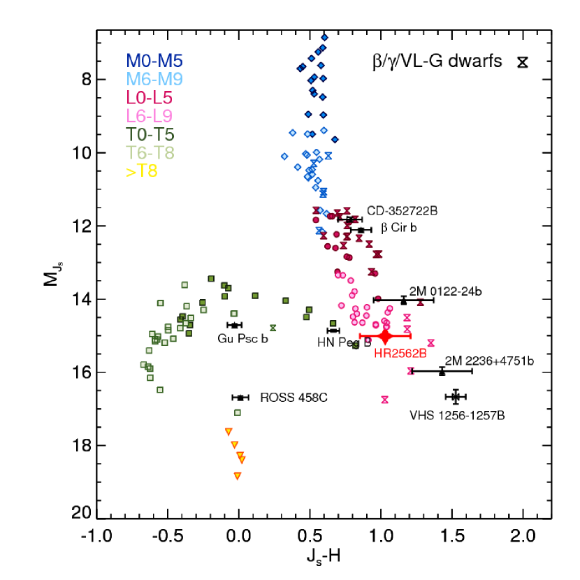
Starting from the photometric values listed in Tab. 3, we have produced the color-magnitude diagram ( -H). The use of the magnitude is justified in this case by the fact that it allows to better discriminate objects near the L/T transition from background contaminants. In this diagram, the position of HR 2562 B is compared to those of M, L and T field dwarfs, whose photometry has been gathered from the flux-calibrated near-infrared spectra from the SpeXPrism library (Burgasser 2014). Like e.g. in Zurlo et al. (2016), we smoothed these spectra to the IRDIS resolution using the IRDIS passbands, a model of the Paranal atmospheric transmission using the ESO Skycalc web application 555http://www.eso.org/observing/etc/bin/gen/form?INS.MODE=swspectr+INS.NAME=SKYCALC(Noll et al. 2012; Jones et al. 2013) and a model spectrum of Vega (Bohlin 2007). We also show the positions of substellar companions with an age comparable to that of HR 2562 B (Luhman et al. 2007; Goldman et al. 2010; Wahhaj et al. 2011; Bowler et al. 2013; Naud et al. 2014; Gauza et al. 2015; Smith et al. 2015; Bowler et al. 2017) as stellar age is known to be a relevant parameter for the spectral and photometric characterization of substellar objects. HR 2562 B sits at the L-T transition, very near to the location of (although slightly redder than) HN Peg B that has comparable age (300-400 Myr) and mass (20MJup), according to Luhman et al. (2007).
5.1.2 Companion parameters through evolutionary models
We estimated the main parameters of the companion using the AMES-COND models (Allard et al. 2003) and the AMES-DUSTY models (Allard et al. 2001), starting from photometry reported in Tab. 3 and assuming the age we have discussed in Sec. 2. The results for the companion mass and its surface gravity are listed in Tab. 4 and in Tab. 5. For these calculations, we adopted three different ages that cover the whole age range proposed in Sec. 2 for HR 2562. The Y and J band results are in good agreement with each other, while the H band determination tends to provide different masses especially in the case of the AMES-COND models. For the intermediate age of 450 Myr the AMES-COND model provides a value of the mass between 20 and 30 MJup (4.7 dex, with in cgs), which is slightly lower than that obtained by Konopacky et al. (2016) because of the younger age adopted in this paper. On the other hand, the AMES-DUSTY model provides a larger value of 40-46 MJup (5.0 dex). These values for the mass are in good agreement with what was recently found from Dupuy & Liu (2017) that, evaluating the dynamical masses of ultracool dwarfes, found for BDs with spectral type around T2-T3 (see Section 5.1.3) a mass range around 30-40 MJup.
| Age | Mass (MJup) | log(g) | ||||
|---|---|---|---|---|---|---|
| (Myr) | Y | J | H | Y | J | H |
| 200 | 11.46 | 11.80 | 18.55 | 4.34 | 4.35 | 4.58 |
| 450 | 20.85 | 22.12 | 29.16 | 4.69 | 4.71 | 4.85 |
| 750 | 27.40 | 28.67 | 37.58 | 4.85 | 4.87 | 5.01 |
| Age | Mass (MJup) | log(g) | ||||
|---|---|---|---|---|---|---|
| (Myr) | Y | J | H | Y | J | H |
| 200 | 34.04 | 32.14 | 28.41 | 4.82 | 4.80 | 4.74 |
| 450 | 46.59 | 44.84 | 40.21 | 5.03 | 5.02 | 4.97 |
| 750 | 56.08 | 54.34 | 49.51 | 5.18 | 5.16 | 5.12 |
5.1.3 Fitting with spectral template
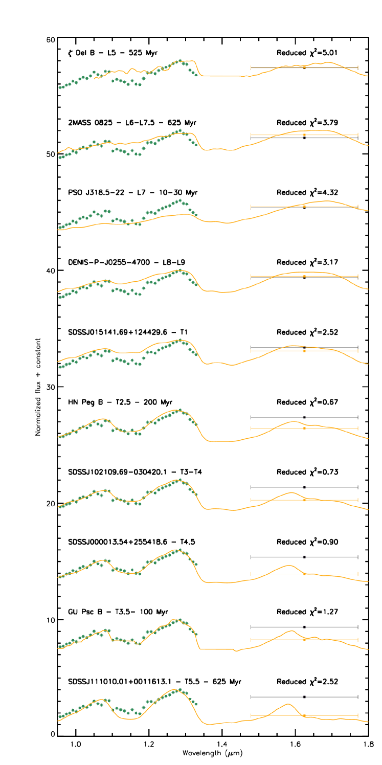
In order to better ascertain the spectral type of HR 2562 B, we have performed fit procedures of its spectrum with sample spectra of field BDs taken from the Spex Prism spectral Libraries666http://pono.ucsd.edu/~adam/browndwarfs/spexprism/ (Burgasser 2014). The final result is displayed in Fig. 6, where we show the comparison of the extracted spectrum for HR 2562 B with those of ten objects having spectral types between L5 and T5 (Burgasser et al. 2004, 2006; Luhman et al. 2007; Cushing et al. 2008; Stephens et al. 2009; Liu et al. 2013; De Rosa et al. 2014; Naud et al. 2014; Gagné et al. 2015). The best fit was obtained with the spectrum of HN Peg B (Luhman et al. 2007) that is classified as T2.5 spectral type. This result confirms what we obtained in Sec. 5.1.1 where we showed (see Fig. 5) that the positions of these two objects are very similar in the color-magnitude diagram. Thus, we found compelling evidence that they could be very similar objects. However, a comparably good fit was also obtained with the spectrum of SDSS J143553.25+112948.6 (Chiu et al. 2006) that was classified as T21 spectral type, and SDSS J102109.69030420.1AB (Burgasser et al. 2006) that was classified as a T3 spectral type. From these results we can define this object as a T2-T3 spectral type. It is noteworthy, however, that the value derived from the IRDIS H broad band data does not agree well with this result. Indeed, looking at the comparison of the flux in H broad band between HR 2562 B and the template spectra represented by the dark and the orange squares in Fig. 6 respectively, our finding seems in better agreement with a late-L spectral type.
5.1.4 Fitting with atmospheric models
To further constrain the physical parameters of HR 2562 B we compared its extracted spectrum to synthetic spectra from different atmospheric models.
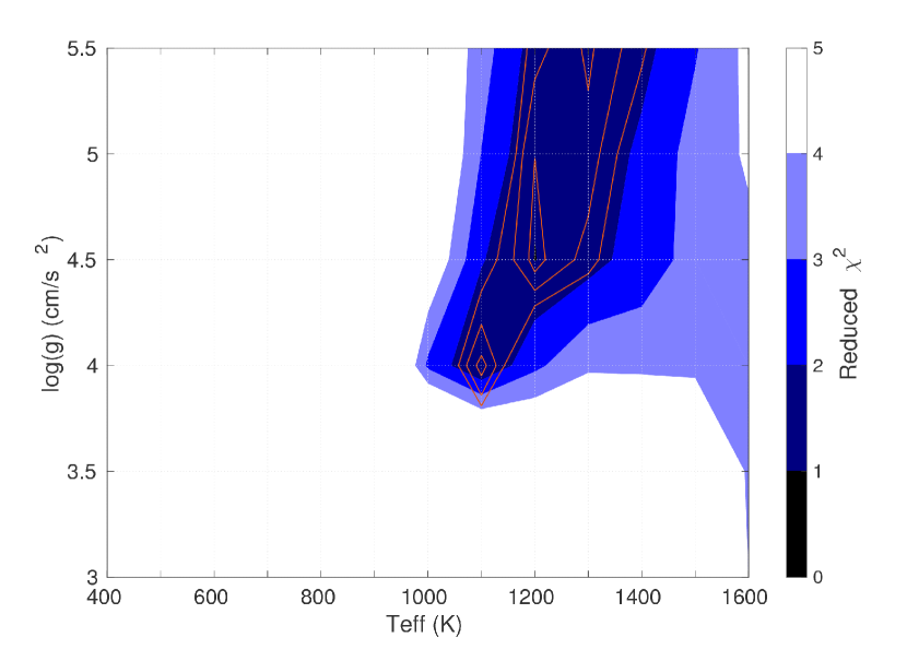
We first used the BT-Settl models (Allard 2014) with a grid covering between 900 and 2500 K with a step of 100 K and a ranging between 2.5 and 5.5 dex, with a step of 0.5. All the models were for a solar metallicity. The results of this procedure are displayed in Fig. 7. The best fit is with the spectrum with =1200 K and =4.5. A good fit is however obtained even for a spectrum with =1100 K and =4.0 and for a spectrum with =1300 K and =5.5. We can then conclude that the fit gives =1200100 K and =. and log(g) values found through this procedure are in good agreement with those found by Konopacky et al. (2016).

As a second step, we have compared the extracted spectrum for HR 2562 B with the Exo-REM model (Baudino et al. 2015), which is specifically developed for young giant exoplanets. We first generated a grid of models with between 400 and 1800 K with a step of 100 K, in the range 2.5-5.5 dex with a step of 0.1, with and without Fe and considering a particle radius of 30 m and assuming equilibrium and non-equilibrium chemistry ( ). All these models were then compared to the spectrum of HR 2562 B to find the one that minimize the . All the values with less than 1 were then considered as acceptable. The best fits obtained from this procedure are shown in the upper panel of Fig. 8, while in the lower panel we show as a comparison an example of a poor quality fit. The best results are for models with in the range 1100-1200 K, 5.0 dex, cloud with an optical depth of =0.5 and non-equilibrium chemistry. However, considering all the models with a value of less than 1 we can only constrain a in the range 950-1200 K and in the range 3.4-5.2 dex

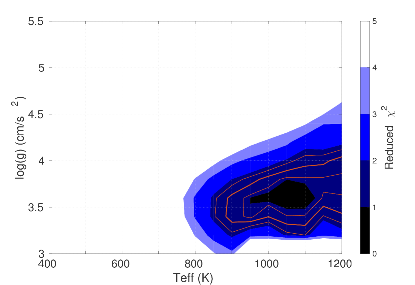
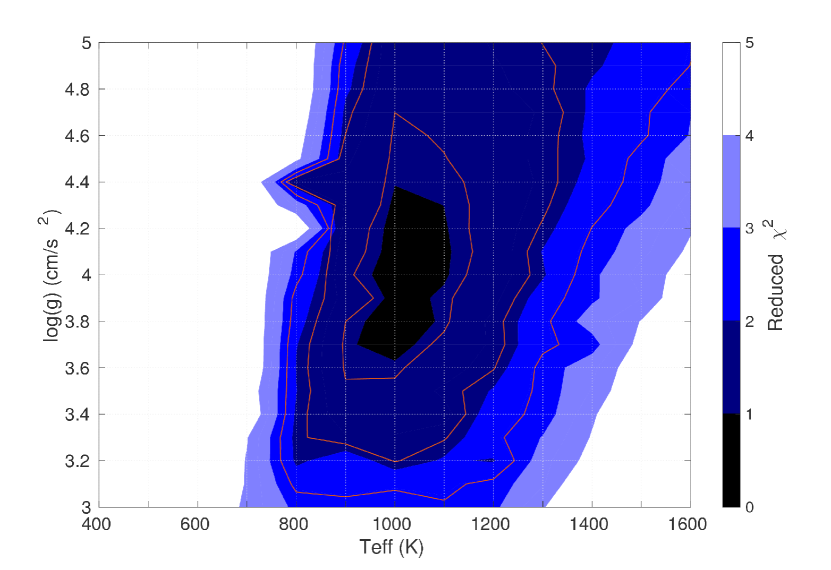
Aiming at carefully evaluate the contribution of the cloud coverage on the definition of the main parameters for the companion, we have also used a new version of the Exo-REM models. This includes a self-consistent modelling of the clouds (both iron and silicate) that is based on the parameterization of the profile, and considers cloud condensation, coalescence, sedimentation and vertical mixing (Charnay et al., in prep.). The size of the cloud particles is calculated by comparing typical timescales for condensation, coalescence, sedimentation and vertical mixing, following the method described in Rossow (1978). Moreover, these models take into account cloud scattering and can also simulate a cloud coverage fraction as done by Marley et al. (2010). The model ranges from 400 to 2000 K with step of 100 K, while varies from 3 to 5 dex, with step of 0.1 dex. We considered models with 0.3, 1 and 3 times the solar metallicity. The decision to explore different metallicities is due to the fact that we have found that the star is slightly metal rich with respect to the Sun (see Section 2.1) and that there are claims in literature about metallicity enhancement of substellar companions with respect to their parent stars (Skemer et al. 2016; Samland et al. 2017). Equilibrium and non-equilibrium chemistry were adopted along with different cloud coverage: the best fitting results in models with non-equilibrium chemistry and a cloud coverage of 95%. The best fit spectra from this procedure are shown in Fig. 9 while the map is displayed in Fig. 10 together with those from BT-Settl and not modified Exo-REM models. The result of this second procedure points toward an object at between 1000 and 1200 K and just above 4.0 dex. Indeed, considering a metallicity three times the solar value, we obtain =1100100 K and =4.30.6 dex, while for a solar metallicity we estimate from the model =900-1150 K and =4.10.6 dex. For what concerns the exploration of the metallicity, instead, no definitive results can be deduced from these models even if models with metallicity lower than solar tend to prefer values of less than 4 while models with metallicity higher than solar tend to prefer values of nearer to the values deduced through evolutionary models.
5.1.5 Comparison of results from evolutionary and atmospheric models
As for , by comparing our data with atmospheric models we have inferred values lower than that obtained from the evolutionary models, in particular when DUSTY models are employed (see Section 5.1.2). This can be explained by the fact that the cloud coverage of the atmosphere of HR 2562 B is likely only partial, as confirmed by the quite compelling evidence provided by the Exo-REM models. However, when we consider the whole atmospheric model data-sets we obtain a wide range of ranging from 3.4 to 5.2. We conclude that it is difficult to firmly constrain the value of by exploiting atmospheric models, because their dependence on gravity is relatively small. From this point of view, the estimates that we gathered using the evolutionary models are much more useful, and with significantly smaller dispersion. In fact, they represents two extreme conditions (absence of clouds in the COND models complete coverage of clouds for the DUSTY case) that can be used to constrain the correct value of . We can then consider the lower and the upper values obtained from these models and listed in Tab. 4 and 5 and use them to estimate the value of as . The main contribution to the error bar is clearly given by the uncertainties on the age of the system. On the other hand, is much better constrained with values in the range 900-1300 K so that we can then assume for a value of K. This is in good agreement with the spectral classification of T2-T3 that we obtained from the procedure described in Section 5.1.3. Indeed, Pecaut & Mamajek (2013) foresee =1200 K for a T2 spectral type and of 1160 K for a T3 spectral type.

5.2 Mass limits for other objects in the system
Starting from the contrast limit displayed in Fig. 3 and using the AMES-COND models (Allard et al. 2003), we have obtained the limit in mass for other possible companions around HR 2562. This is shown in Fig. 11, where the solid lines are obtained assuming an age of 450 Myr. Moreover, with the aim to show the dependency of the limits from the age, we display in dashed lines the mass limits that are obtained assuming 200 and 750 Myr (these are the lower and upper limits proposed for the age). From our findings we should be able to see objects with mass of the order of 10MJup at separations larger than 10 au, while at separation larger than 40 au IRDIS should allow us to detect objects with masses of few MJup.

6 Conclusions
In this paper we have presented the high-contrast imaging observations of the star HR 2562 obtained with SPHERE. We were able to recover the low-mass companion previously discovered by Konopacky et al. (2016) both with IRDIS and IFS.
Using the companion photometry extracted in the Y, J and H band and the AMES-COND evolutionary models, we derived a mass in the 20-30 MJup range and a 4.7 dex. Conversely, by adopting the AMES-DUSTY models we obtained larger masses ( 40 MJup) and of 5.0 dex.
The spectro-photometric measurements performed with IFS allowed us to extract a low-resolution spectrum of the companion in Y and J band, while IRDIS provided us H broad-band photometry. Fitting the extracted spectrum with a sample of spectra of low mass objects, we were able to classify HR 2562 B as an early T (T2-T3) spectral type, although the H broad-band photometry seems more in accordance with late-L spectra. Our spectral classification is then not in complete accordance with that by Konopacky et al. (2016). The IFS spectrum is very similar to that obtained by GPI in the J band so that the different spectral classification is probably due to the different spectral coverage of the two instruments, outside the J band. In fact, the extension to the Y band allows to SPHERE to see the peak at 1.08 m (not visible in GPI), making possible to identify the early-T nature of the object. On the other hand, the GPI spectrum by Konopacky et al. (2016) extends to the H and K band; their classification was mainly based on the H and K band observations. Thus, while the presence of the peak at 1.08 m in the IFS spectrum strongly points towards an early-T type spectrum, several uncertainties still remain and observations on a wider wavelength range are sorely needed to completely disentangle the companion spectral classification.
It is also possible that some variability affects the spectral appareance of HR 2562 B. Indeed, photometric variability due to non-uniform cloud coverage has been shown to be more prominent for L/T transition objects (see e.g. Buenzli et al. 2014; Metchev et al. 2015).
The use of synthetic spectra from atmospheric models allowed us to put some constraints on the physical parameters of the companion. Using the BT-Settl models, the best solution was found for =1200100 K and =4.50.5 dex. The Exo-REM models allowed us to define a range of 950-1200 K for and of 3.4-5.2 for , with strong indications for the upper limit of these intervals. Finally, we have used for our analysis a new version of the Exo-REM models, which are modified to have a self-consistent treatment of the clouds. In this case our findings suggest a in the range 1000-1200 K and a lower than that found by the other models (of the order of 4.0 dex). However, both the Exo-REM models give strong hints of the presence of clouds with a high cloud coverage (best fit of 95%) and non-equilibrium chemistry.
Synthetizing all the results described in the paper, HR 2562 B should have a mass of MJup with = K and =.
Acknowledgements.
The authors thanks Quinn Konopacky for sharing the GPI spectra of HR 2562 B. We are grateful to the SPHERE team and all the people at Paranal for the great effort during SPHERE GTO run. This work has made use of the SPHERE Data Center, jointly operated by OSUG/IPAG (Grenoble), PYTHEAS/LAM/CeSAM (Marseille), OCA/Lagrange (Nice) and Observatoire de Paris/LESIA (Paris). D.M. acknowledges support from the ESO-Government of Chile Joint Comittee program ’Direct imaging and characterization of exoplanets’. D.M., A.Z., V.D.O., R.G., R.U.C., S.D., C.L. acknowledge support from the “Progetti Premiali” funding scheme of the Italian Ministry of Education, University, and Research. J.H. is supported by the French ANR through the GIPSE grant ANR-14-CE33-0018. This work has been supported by the project PRIN-INAF 2016 The Cradle of Life - GENESIS-SKA (General Conditions in Early Planetary Systems for the rise of life with SKA). We acknowledge support from the French National Research Agency (ANR) through the GUEPARD project grant ANR10-BLANC0504-01. SPHERE is an instrument designed and built by a consortium consisting of IPAG (Grenoble, France), MPIA (Heidelberg, Germany), LAM (Marseille, France), LESIA (Paris, France), Laboratoire Lagrange (Nice, France), INAF– Osservatorio di Padova (Italy), Observatoire de Genève (Switzerland), ETH Zurich (Switzerland), NOVA (Netherlands), ONERA (France) and ASTRON (Netherlands), in collaboration with ESO. SPHERE was funded by ESO, with additional contributions from CNRS (France), MPIA (Germany), INAF (Italy), FINES (Switzerland) and NOVA (Netherlands). SPHERE also received funding from the European Commission Sixth and Seventh Framework Programmes as part of the Optical Infrared Coordination Network for Astronomy (OPTICON) under grant number RII3-Ct-2004-001566 for FP6 (2004-2008), grant number 226604 for FP7 (2009-2012) and grant number 312430 for FP7 (2013-2016). This research has benefited from the SpeX Prism Spectral Libraries, maintained by Adam Burgasser at http://pono.ucsd.edu/ adam/browndwarfs/spexprismReferences
- Allard (2014) Allard, F. 2014, in IAU Symposium, Vol. 299, Exploring the Formation and Evolution of Planetary Systems, ed. M. Booth, B. C. Matthews, & J. R. Graham, 271–272
- Allard et al. (2003) Allard, F., Guillot, T., Ludwig, H.-G., et al. 2003, in IAU Symposium, Vol. 211, Brown Dwarfs, ed. E. Martín, 325
- Allard et al. (2001) Allard, F., Hauschildt, P. H., Alexander, D. R., Tamanai, A., & Schweitzer, A. 2001, ApJ, 556, 357
- Allard et al. (2012) Allard, F., Homeier, D., & Freytag, B. 2012, Philosophical Transactions of the Royal Society of London Series A, 370, 2765
- Andersen et al. (1985) Andersen, J., Nordstrom, B., Ardeberg, A., et al. 1985, A&AS, 59, 15
- Asiain et al. (1999) Asiain, R., Figueras, F., Torra, J., & Chen, B. 1999, A&A, 341, 427
- Bailey et al. (2014) Bailey, V., Meshkat, T., Reiter, M., et al. 2014, ApJ, 780, L4
- Balachandran (1995) Balachandran, S. 1995, ApJ, 446, 203
- Baudino et al. (2015) Baudino, J.-L., Bézard, B., Boccaletti, A., et al. 2015, A&A, 582, A83
- Beuzit et al. (2008) Beuzit, J.-L., Feldt, M., Dohlen, K., et al. 2008, in Proc. SPIE, Vol. 7014, Ground-based and Airborne Instrumentation for Astronomy II, 701418
- Biller et al. (2010) Biller, B. A., Liu, M. C., Wahhaj, Z., et al. 2010, ApJ, 720, L82
- Boesgaard et al. (1988) Boesgaard, A. M., Budge, K. G., & Ramsay, M. E. 1988, ApJ, 327, 389
- Boesgaard & Tripicco (1986) Boesgaard, A. M. & Tripicco, M. J. 1986, ApJ, 302, L49
- Bohlin (2007) Bohlin, R. C. 2007, in Astronomical Society of the Pacific Conference Series, Vol. 364, The Future of Photometric, Spectrophotometric and Polarimetric Standardization, ed. C. Sterken, 315
- Bonnefoy (2015) Bonnefoy, M. 2015, in AAS/Division for Extreme Solar Systems Abstracts, Vol. 3, AAS/Division for Extreme Solar Systems Abstracts, 203.05
- Bonnefoy et al. (2016) Bonnefoy, M., Zurlo, A., Baudino, J. L., et al. 2016, A&A, 587, A58
- Bowler et al. (2017) Bowler, B. P., Liu, M. C., Mawet, D., et al. 2017, AJ, 153, 18
- Bowler et al. (2013) Bowler, B. P., Liu, M. C., Shkolnik, E. L., & Dupuy, T. J. 2013, ApJ, 774, 55
- Bressan et al. (2012) Bressan, A., Marigo, P., Girardi, L., et al. 2012, MNRAS, 427, 127
- Buenzli et al. (2014) Buenzli, E., Apai, D., Radigan, J., Reid, I. N., & Flateau, D. 2014, ApJ, 782, 77
- Burgasser (2014) Burgasser, A. J. 2014, in Astronomical Society of India Conference Series, Vol. 11, Astronomical Society of India Conference Series
- Burgasser et al. (2006) Burgasser, A. J., Geballe, T. R., Leggett, S. K., Kirkpatrick, J. D., & Golimowski, D. A. 2006, ApJ, 637, 1067
- Burgasser et al. (2004) Burgasser, A. J., McElwain, M. W., Kirkpatrick, J. D., et al. 2004, AJ, 127, 2856
- Casagrande et al. (2011) Casagrande, L., Schönrich, R., Asplund, M., et al. 2011, A&A, 530, A138
- Chauvin et al. (2004) Chauvin, G., Lagrange, A.-M., Dumas, C., et al. 2004, A&A, 425, L29
- Chauvin et al. (2005) Chauvin, G., Lagrange, A.-M., Zuckerman, B., et al. 2005, A&A, 438, L29
- Chen et al. (2014) Chen, C. H., Mittal, T., Kuchner, M., et al. 2014, ApJS, 211, 25
- Chilcote et al. (2017) Chilcote, J., Pueyo, L., De Rosa, R. J., et al. 2017, AJ, 153, 182
- Chiu et al. (2006) Chiu, K., Fan, X., Leggett, S. K., et al. 2006, AJ, 131, 2722
- Claudi et al. (2008) Claudi, R. U., Turatto, M., Gratton, R. G., et al. 2008, in Society of Photo-Optical Instrumentation Engineers (SPIE) Conference Series, Vol. 7014, Society of Photo-Optical Instrumentation Engineers (SPIE) Conference Series
- Cushing et al. (2008) Cushing, M. C., Marley, M. S., Saumon, D., et al. 2008, ApJ, 678, 1372
- da Silva et al. (2006) da Silva, L., Girardi, L., Pasquini, L., et al. 2006, A&A, 458, 609
- de Medeiros & Mayor (1999) de Medeiros, J. R. & Mayor, M. 1999, A&AS, 139, 433
- De Rosa et al. (2014) De Rosa, R. J., Patience, J., Ward-Duong, K., et al. 2014, MNRAS, 445, 3694
- De Rosa et al. (2016) De Rosa, R. J., Rameau, J., Patience, J., et al. 2016, ApJ, 824, 121
- Delorme et al. (2017) Delorme, P., Schmidt, T., Bonnefoy, M., et al. 2017, ArXiv e-prints
- Desidera et al. (2015) Desidera, S., Covino, E., Messina, S., et al. 2015, A&A, 573, A126
- Desidera et al. (2011) Desidera, S., Covino, E., Messina, S., et al. 2011, A&A, 529, A54
- Dohlen et al. (2008) Dohlen, K., Langlois, M., Saisse, M., et al. 2008, in Society of Photo-Optical Instrumentation Engineers (SPIE) Conference Series, Vol. 7014, Society of Photo-Optical Instrumentation Engineers (SPIE) Conference Series
- D’Orazi et al. (2017) D’Orazi, V., Desidera, S., Gratton, R. G., et al. 2017, A&A, 598, A19
- Dupuy & Liu (2017) Dupuy, T. J. & Liu, M. C. 2017, ApJS, 231, 15
- Gagné et al. (2015) Gagné, J., Burgasser, A. J., Faherty, J. K., et al. 2015, ApJ, 808, L20
- Gagné et al. (2014) Gagné, J., Lafrenière, D., Doyon, R., Malo, L., & Artigau, É. 2014, ApJ, 783, 121
- Garcia et al. (2017) Garcia, E. V., Currie, T., Guyon, O., et al. 2017, ApJ, 834, 162
- Gauza et al. (2015) Gauza, B., Béjar, V. J. S., Pérez-Garrido, A., et al. 2015, ApJ, 804, 96
- Goldman et al. (2010) Goldman, B., Marsat, S., Henning, T., Clemens, C., & Greiner, J. 2010, MNRAS, 405, 1140
- Gray et al. (2006) Gray, R. O., Corbally, C. J., Garrison, R. F., et al. 2006, AJ, 132, 161
- Johnson-Groh et al. (2017) Johnson-Groh, M., Marois, C., De Rosa, R. J., et al. 2017, AJ, 153, 190
- Jones et al. (2013) Jones, A., Noll, S., Kausch, W., Szyszka, C., & Kimeswenger, S. 2013, A&A, 560, A91
- Konopacky et al. (2016) Konopacky, Q. M., Rameau, J., Duchêne, G., et al. 2016, ApJ, 829, L4
- Lagrange et al. (2010) Lagrange, A.-M., Bonnefoy, M., Chauvin, G., et al. 2010, Science, 329, 57
- Langlois et al. (2013) Langlois, M., Vigan, A., Moutou, C., et al. 2013, in Proceedings of the Third AO4ELT Conference, ed. S. Esposito & L. Fini, 63
- Liu et al. (2013) Liu, M. C., Magnier, E. A., Deacon, N. R., et al. 2013, ApJ, 777, L20
- Luhman et al. (2007) Luhman, K. L., Patten, B. M., Marengo, M., et al. 2007, ApJ, 654, 570
- Macintosh et al. (2015) Macintosh, B., Graham, J. R., Barman, T., et al. 2015, Science, 350, 64
- Macintosh et al. (2014) Macintosh, B., Graham, J. R., Ingraham, P., et al. 2014, Proceedings of the National Academy of Science, 111, 12661
- Maire et al. (2016) Maire, A.-L., Bonnefoy, M., Ginski, C., et al. 2016, A&A, 587, A56
- Marley et al. (2010) Marley, M. S., Saumon, D., & Goldblatt, C. 2010, ApJ, 723, L117
- Marois et al. (2014) Marois, C., Correia, C., Galicher, R., et al. 2014, in Proc. SPIE, Vol. 9148, Adaptive Optics Systems IV, 91480U
- Marois et al. (2006a) Marois, C., Lafrenière, D., Doyon, R., Macintosh, B., & Nadeau, D. 2006a, ApJ, 641, 556
- Marois et al. (2006b) Marois, C., Lafrenière, D., Macintosh, B., & Doyon, R. 2006b, ApJ, 647, 612
- Marois et al. (2008) Marois, C., Macintosh, B., Barman, T., et al. 2008, Science, 322, 1348
- Mesa et al. (2015) Mesa, D., Gratton, R., Zurlo, A., et al. 2015, A&A, 576, A121
- Mesa et al. (2016) Mesa, D., Vigan, A., D’Orazi, V., et al. 2016, A&A, 593, A119
- Metchev et al. (2015) Metchev, S. A., Heinze, A., Apai, D., et al. 2015, ApJ, 799, 154
- Milli et al. (2017) Milli, J., Hibon, P., Christiaens, V., et al. 2017, A&A, 597, L2
- Montes et al. (2001) Montes, D., López-Santiago, J., Gálvez, M. C., et al. 2001, MNRAS, 328, 45
- Moór et al. (2006) Moór, A., Ábrahám, P., Derekas, A., et al. 2006, ApJ, 644, 525
- Moór et al. (2015) Moór, A., Kóspál, Á., Ábrahám, P., et al. 2015, MNRAS, 447, 577
- Moór et al. (2011) Moór, A., Pascucci, I., Kóspál, Á., et al. 2011, ApJS, 193, 4
- Naud et al. (2014) Naud, M.-E., Artigau, É., Malo, L., et al. 2014, ApJ, 787, 5
- Noll et al. (2012) Noll, S., Kausch, W., Barden, M., et al. 2012, A&A, 543, A92
- Nordström et al. (2004) Nordström, B., Mayor, M., Andersen, J., et al. 2004, A&A, 418, 989
- Pace (2013) Pace, G. 2013, A&A, 551, L8
- Pavlov et al. (2008) Pavlov, A., Möller-Nilsson, O., Feldt, M., et al. 2008, in Society of Photo-Optical Instrumentation Engineers (SPIE) Conference Series, Vol. 7019, Society of Photo-Optical Instrumentation Engineers (SPIE) Conference Series, 39
- Pecaut & Mamajek (2013) Pecaut, M. J. & Mamajek, E. E. 2013, ApJS, 208, 9
- Rajan et al. (2017) Rajan, A., Rameau, J., De Rosa, R. J., et al. 2017, AJ, 154, 10
- Rameau et al. (2013) Rameau, J., Chauvin, G., Lagrange, A.-M., et al. 2013, ApJ, 779, L26
- Rhee et al. (2007) Rhee, J. H., Song, I., Zuckerman, B., & McElwain, M. 2007, ApJ, 660, 1556
- Rossow (1978) Rossow, W. B. 1978, Icarus, 36, 1
- Samland et al. (2017) Samland, M., Mollière, P., Bonnefoy, M., et al. 2017, A&A, 603, A57
- Sivaramakrishnan & Oppenheimer (2006) Sivaramakrishnan, A. & Oppenheimer, B. R. 2006, ApJ, 647, 620
- Skemer et al. (2016) Skemer, A. J., Morley, C. V., Zimmerman, N. T., et al. 2016, ApJ, 817, 166
- Smith et al. (2015) Smith, L. C., Lucas, P. W., Contreras Peña, C., et al. 2015, MNRAS, 454, 4476
- Soummer et al. (2012) Soummer, R., Pueyo, L., & Larkin, J. 2012, ApJ, 755, L28
- Stauffer et al. (2016) Stauffer, J., Rebull, L., Bouvier, J., et al. 2016, AJ, 152, 115
- Steinhauer & Deliyannis (2004a) Steinhauer, A. & Deliyannis, C. P. 2004a, ApJ, 614, L65
- Steinhauer & Deliyannis (2004b) Steinhauer, A. & Deliyannis, C. P. 2004b, ApJ, 614, L65
- Stephens et al. (2009) Stephens, D. C., Leggett, S. K., Cushing, M. C., et al. 2009, ApJ, 702, 154
- Valenti & Piskunov (1996) Valenti, J. A. & Piskunov, N. 1996, A&AS, 118, 595
- Vigan et al. (2016) Vigan, A., Bonnefoy, M., Ginski, C., et al. 2016, A&A, 587, A55
- Vigan et al. (2010) Vigan, A., Moutou, C., Langlois, M., et al. 2010, MNRAS, 407, 71
- Wahhaj et al. (2011) Wahhaj, Z., Liu, M. C., Biller, B. A., et al. 2011, ApJ, 729, 139
- Zuckerman & Song (2004) Zuckerman, B. & Song, I. 2004, ARA&A, 42, 685
- Zurlo et al. (2016) Zurlo, A., Vigan, A., Galicher, R., et al. 2016, A&A, 587, A57
- Zurlo et al. (2014) Zurlo, A., Vigan, A., Mesa, D., et al. 2014, A&A, 572, A85