Structure of partially hyperbolic Hénon maps

Abstract.

We consider the structure of substantially dissipative complex Hénon maps admitting a dominated splitting on the Julia set. The dominated splitting assumption corresponds to the one-dimensional assumption that there are no critical points on the Julia set. Indeed, we prove the corresponding description of the Fatou set, namely that it consists of only finitely many components, each either attracting or parabolic periodic. In particular there are no rotation domains, and no wandering components. Moreover, we show that $J=J^{\star}$ and the dynamics on $J$ is hyperbolic away from parabolic cycles.

1. Introduction

Complex Hénon maps are polynomial automorphisms of $\mathbb{C}^{2}$ with non-trivial dynamical behavior,

$$f:(x,y)\mapsto(p(x)-by,x),\quad{\mathrm{where}}\ \deg p\geq 2,\ b=\operatorname{Jac}f\not=0.$$

For a small Jacobian $b$, it can be viewed as a perturbation of the one-dimensional polynomial $p:\mathbb{C}\rightarrow\mathbb{C}$. Though some initial aspects of the 2D theory resembles the 1D theory, quite quickly it becomes much more difficult, exhibiting various new phenomena.

Dynamics of 1D polynomials on the Fatou set is fully understood, due to the classical work of Fatou, Julia and Siegel, supplemented with Sullivan’s No Wandering Domains Theorem from the early ’80s [Su85] . This direction of research for Hénon maps was initiated by Bedford and Smillie in the early ’90’s. In particular, they gave a description of the dynamics on “recurrent” periodic Fatou components [BS91b]. The “non-recurrent” case was recently treated by the authors [LP14], under an assumption that the Hénon map is “substantially dissipative”, i.e.

$$\left|\mathrm{\operatorname{Jac}}f\right|<\frac{1}{(\deg p)^{2}}.$$

It completed the classification of periodic Fatou components in this setting: Any such component is either an attracting or parabolic basin, or a rotation domain, which is analogous to the one-dimensional classification.

The situation with the problem of wandering components is more complicated. In fact, wandering Fatou components can exist for polynomial endomorphisms $g:\mathbb{C}^{2}\rightarrow\mathbb{C}^{2}$, as was recently demonstrated in [ABDPR16]. It is probable that wandering components can exist for Hénon maps as well, but one can hope that “generically” they do not.

It is quite clear that Sullivan’s proof of the Non-Wandering Domains Theorem, based upon quasiconformal deformations machinery, is not generalizable to higher dimensions. At the same time, for various special classes of 1D polynomial maps, one can give a direct geometric argument that has a chance to be generalized to the 2D setting. The simplest class of this kind comprises hyperbolic polynomials, for which absence of wandering component was known classically. The Hénon counterpart of this result was established by Bedford and Smillie in the ’90s, resulting in a complete description of the dynamics on the Fatou set for this class [BS91a]: a hyperbolic Hénon map has only finitely many Fatou components, each of which is an attracting basin. Moreover, in this case, the Julia set $J$ is the closure of saddles: $J=J^{*}$.

Until now, hyperbolic maps remained the only class of Hénon maps for which these problems were settled down. In this paper, we are making one step further, resolving these problems for substantially dissipative Hénon maps that admit a “dominated splitting” over the Julia set:

Theorem 1.1.

Let $f:\mathbb{C}^{2}\rightarrow\mathbb{C}^{2}$ be a substantially dissipative Hénon map that admits a dominated splitting over the Julia set $J$. Then:

$\bullet$ $f$ does not have wandering Fatou components;

$\bullet$ $f$ has only finitely many periodic Fatou components, each being either an attracting or a parabolic basin;

$\bullet$ $J=J^{*}$, i.e., the Julia set is the closure of saddles.

Hénon maps with dominated splitting are 2D counterparts of 1D polynomial maps without critical points on the Julia set. Our initial observation was that for such a polynomial, the No Wandering Domains Theorem can be proven by means of Mañé’s techniques (refined in [CYJ94] and [STL00]) treating maps with non-recurrent critical points. However, an adaptation of these techniques to the Hénon setting is not straightforward: in particular, it required to impose an assumption of substantial dissipativity, to develop an appropriate version of the $\lambda$-lemma, and to bound the iterated degrees of wandering components.

The main work in this paper is to show that, away from the parabolic cycles, $f$ is expanding in the horizontal direction. (In particular, if there are no parabolic cycles then $f$ is hyperbolic.) The non-existence of wandering Fatou components and periodic rotation domains follows easily, and it also follows that $J=J^{*}$. Moreover, we show that if there are parabolic cycles, then $f$ lies on the boundary of the hyperbolicity locus, at least when viewed in the parameter space of Hénon-like maps.

Non-hyperbolic complex Hénon maps admitting a dominated splitting have been constructed by Radu and Tanase [RT14]. These examples are perturbations of 1D parabolic polynomials.

The structure of the paper is as follows. In section (2) we will review Mañé’s Theorem analysing the dynamics of 1D polynomials without recurrent critical points (except possible superattracting cycles). We give a detailed proof that follows ideas from a paper of Shishikura and Tan Lei [STL00]. However, we have chosen to present an argument that will be a closest possible model to the two-dimensional proof we give later. This means that the one-dimensional argument is not the most efficient. For instance, naturally we do not assume the non-existence of wandering components.

In section (3) we recall Hénon maps and the substantial dissipativity condition, and in section (4) we define the dominated splitting and make some elementary observations. The dominated splitting on $J$ induces a lamination on $J^{+}\cap\Delta^{2}_{R}$ by vertical disks. In section (5) this lamination is extended to a neighborhood of $J^{+}$, introducing the artificial vertical lamination. While this lamination is not invariant, it plays an important role in our proofs.

In wandering Fatou components we can consider both the artificial and the dynamical lamination given by strong stable manifolds. These two laminations may not agree on orbits of wandering domains that leave the region of dominated splitting, leading to interpretations of degree, discussed in sections (6) and (7).

In section (8) we make the final preparations and in section (9) we prove the main technical result, Proposition 9.3. In section (10) we prove the consequences of this proposition, including Theorem 1.1 above.

In conclusion, let us note that dominated splitting is an important classical notion going back to the works of Pliss and Mañé from the ’70s. Dynamics of real surface diffeomorphisms with dominated splitting was described by Pujals and Samborino [PS09]. This result inspired our work.

Acknowledgment. It is our pleasure to thank Enrique Pujals, Vladlen Timorin, Remus Radu and Raluca Tanase for very interesting discussions of the dominated splitting theme. This work has been partially supported by the NSF, NSERC, and the Simons Foundation.

2. The one-dimensional argument

Let $f:\mathbb{C}\rightarrow\mathbb{C}$ be a polynomial, and assume that there are no critical points on $J$, the Julia set of $f$. We let $\Omega$ be a backward invariant open neighborhood of $J\setminus\{parabolics\}$, constructed by removing closed forward invariant sets from a finite number of (pre-) periodic Fatou components. We will assume that $\Omega$ is arbitrarily thin, i.e. contained in an arbitrarily small neighborhood of the union of $J\setminus\{parabolics\}$ with the wandering Fatou components.

The wandering Fatou components can contain only a finite number of critical points $x_{1},\ldots,x_{\nu}$, having respective local degrees $d_{1},\ldots,d_{\nu}$. We denote

$$\mathrm{deg}_{\mathrm{crit}}=\prod_{s=1}^{\nu}d_{s}.$$

The constant $\mathrm{deg}_{\mathrm{crit}}$ functions as a maximal local degree on the wandering components for all iterates, i.e. if $V^{0},V^{1},\ldots,V^{n}$ is a orbit of open connected sets, each $V^{n}$ is contained in a wandering domain and has sufficiently small Euclidean diameter, then $f^{n}:V^{0}\rightarrow V^{n}$ has degree at most $\mathrm{deg}_{\mathrm{crit}}$.

We will use the following shorthand notation. For a connected set $V$, we denote by $V^{-j}$ a connected component of $f^{-j}(V)$. If $V\subset W$ then we will always assume that $V^{-j}\subset W^{-j}$. When working with both $V^{-i}$ and $V^{-j}$, for $j>i$, we will assume that $f^{j-i}(V^{-j})=V^{-i}$, i.e. that $V^{-i}$ and $V^{-j}$ are contained in the same backward orbit.

We will show that there exist an integer $M\in\mathbb{N}$ such that the following holds whenever $\Omega$ is sufficiently thin.

Proposition 2.1.

Let $z\in\Omega$ and let $r>0$ be such that $D_{M\cdot r}(z)\subset\Omega$. Then for every $j\in\mathbb{N}$ we have that

$$\mathrm{\bf deg}(j): \;\;\;\;\;\mathrm{deg}\left(f^{j}:D^{-j}_{r}(z)\rightarrow D_{r}(z)\right)\leq\mathrm{deg}_{\mathrm{crit}},$$

$$\mathrm{\bf diam}(j): \;\;\;\;\;\mathrm{diam}_{\Omega}D^{-j}_{r}(z)\leq N_{0}(2K)\cdot C(\frac{1}{2},\mathrm{deg}_{\mathrm{crit}}).$$

The constants $C(\cdot,\cdot)$ and $N_{0}(\cdot)$ will be introduced in Lemmas 2.2 and 2.4 below.

Our proof will closely resemble the proof of a theorem of Mañé, presented in [STL00]. In fact, readers familiar with this reference will likely find our proof needlessly complicated. The reason for these complications is that the proof given here will model the forthcoming $2$-dimensional proof. In particular, we will not use that there are no wandering domains. In fact, the non-existence of wandering domains follows, in our setting, from the above Proposition. The a priori possibility of wandering domains makes the proof significantly more involved.

The fact that Fatou components of one-dimensional polynomials are simply connected is quite useful when dealing with degrees. It follows that if a Fatou component $U$ does not contain critical points, then $f:U\rightarrow f(U)$ is univalent. This is another fact that we will not be able to use in higher dimensions, so we will not use it here either. In this respect the setting is more analogous to the iteration of rational functions, where Fatou components may not be simply connected. An elementary proof however shows that for every wandering component $U$ there exists an $N\in\mathbb{N}$ such that $f^{n}(U)$ is simply connected for $n\geq N$, a result known as Baker’s Lemma, see for example [Za]. Thus, if such $f^{n}(U)$ does not contain critical points, then $f:f^{n}(U)\rightarrow f^{n+1}(U)$ is univalent. We can use the fact that $f:f^{n}(U)\rightarrow f^{n+1}(U)$ is univalent for $n$ large enough, as we will prove the corresponding statement for Hénon maps. Note that nowhere else in the one-dimensional argument will we use simple connectivity to conclude univalence.

A third difference with the argument in [STL00] concerns the induction procedure. Instead of applying the induction hypothesis to $f^{n}:D^{-n}_{r}(z)\rightarrow D_{r}(z)$, and then mapping backward one more step with $f:D^{-n-1}_{r}(z)\rightarrow D^{-n}_{r}(z)$, we will first apply one iterate $f:D^{-1}_{r}(z)\rightarrow D_{r}(z)$, cover $D^{-1}_{r}(z)$ with smaller disks $D_{r_{k}}(z_{k})$, and applying the induction hypothesis to each $f^{n}:D^{-n}_{r_{k}}(z_{k})\rightarrow D_{r_{k}}(z_{k})$. The reason for this will become apparent when the proof is discussed in the Hénon setting.

2.1. Preliminaries

The following basic lemma (see e.g., [LM99, STL00]) will be used repeatedly:

Lemma 2.2.

Let $d\in\mathbb{N}$ and $r>0$. Then there exists a constant $C(r,d)>0$ such that for every proper holomorphic map $f:\mathbb{D}\rightarrow\mathbb{D}$ of degree at most $d$, every connected component of $f^{-1}D_{r}(0)$ has hyperbolic diameter at most $C(r,d)$. Moreover, $C(r,d)\rightarrow 0$ as $r\rightarrow 0$.

The first step in the proof is the construction of the backwards domain $\Omega$ where the argument of 2.1 will take place.

Lemma 2.3.

Given any $\epsilon>0$, there exists a backward invariant domain $\Omega$ contained in the $\epsilon$-neighborhood of

$$\left(J\setminus\{\text{parabolic cycles}\}\right)\cup\left(\bigcup\text{wandering domains}\right),$$

which further has the property that for every $z\in J$ there exist points $w\notin\Omega$ with $|z-w|<\epsilon$.

Proof.

We are done if we can remove sufficiently large forward invariant subsets from a finite number of (pre-) periodic Fatou components. By the classification of periodic Fatou components those periodic components are either attracting basins, parabolic basins or Siegel domains. In an immediate basin of an attracting periodic cycle we can construct an arbitrarily large forward invariant compact subset. In a cycle of Siegel domains we can find an arbitrarily large completely invariant compact subset. Finally, in a cycle of parabolic domains we can find an arbitrarily large forward invariant compact subset that intersects $J$ only in parabolic fixed points. By taking the union of sufficiently large preimages of these subsets we obtain a forward invariant compact subset $K$ disjoint from $J\setminus\{\text{parabolic cycles}\}$, for which $\Omega=\mathbb{C}\setminus K$ satisfies the conditions required in the lemma. ∎

The domain $\Omega$ will later be fixed for a constant $\epsilon>0$ chosen sufficiently small. In particular, we may assume that the only critical points in $\Omega$ lie in wandering Fatou components.

Lemma 2.4.

For each $t>1$ there exists an integer $N_{0}=N_{0}(t)$ such that for every disk $D_{r}(z)\subset D_{t\cdot r}(z)\subset\Omega$ we can cover $D^{-1}_{r}(z)$ with at most $N_{0}$ disks $D_{r_{k}}(z_{k})$ satisfying

$$D_{2t\cdot r_{k}}(z_{k})\subset\Omega.$$

If $D_{t\cdot r}(z)$ is contained in a wandering domain $U^{0}$, then the disks $D_{t\cdot r_{k}}(z_{k})$ can be chosen so that

$$D_{2t\cdot r_{k}}(z_{k})\subset U^{-1}.$$

In all other cases the disks $D_{t\cdot r_{k}}(z_{k})$ can be chosen so that

$$D_{2t\cdot r_{k}}(z_{k})\subset D_{t\cdot r}^{-1}(z).$$

Proof.

If $D_{r}(z)$ is sufficiently small and close to a critical point, it must be contained in a wandering Fatou component $U$. The statement follows immediately.

For sufficiently small disks bounded away from critical values the existence of a uniform bound is clear, as the map $f:D_{t\cdot r}^{-1}(z)\rightarrow D_{t\cdot r}(z)$ is close to linear. Therefore it is sufficient to consider disks $D_{r}(z)\subset D_{t\cdot r}(z)$ of radius bounded away from zero. This is a compact family of disks, hence the existence of a uniform $N_{0}$ is immediate. ∎

We note that while $N_{0}(t)$ will play a similar role as the constant $N_{0}$ in [STL00], its definition differs as the disks $D_{r_{k}}(z_{k})$ cover a preimage $D^{-1}_{r}(z)$ instead of the original $D_{r}(z)$. In particular, the constant $N_{0}$ from [STL00] is a universal, while the constants $N_{0}(t)$ introduced here depend on $f$.

Remark 2.5.

Since the disks $D_{2t\cdot r_{k}}(z)$ are contained in either a wandering domain $U^{-1}$ or in the preimage $D_{t\cdot k}^{-1}(z)$, it follows that the constant $N_{0}(t)$ does not depend on $\Omega$. To be more precise, when $\Omega$ is made smaller, the constant $N_{0}(t)$ does not need to be changed.

The domain $\Omega$ is a Riemann surface whose universal cover is the unit disk, hence $\Omega$ is equipped with a Poincaré metric $d_{\Omega}$. We will prove that all inverse branches $D^{-i}_{r}(z)$ of sufficiently protected disks, i.e. disks $D_{r}(z)\subset D_{2K\cdot r}(z)\subset\Omega$ for a sufficiently large constant $K$ to be determined later, have Poincaré diameter bounded by

$$\mathrm{diam}_{\mathrm{max}}:=N_{0}(2K)\cdot C(\frac{1}{2},\mathrm{deg}_{\mathrm{crit}}).$$

By choosing $\Omega$ sufficiently thin, i.e. the constant $\epsilon$ in Lemma 2.3 sufficiently small, it therefore follows that the Euclidean diameter of each $D^{-i}_{r}(z)$ is arbitrarily small, unless $D^{-i}_{r}(z)$ is contained in a wandering Fatou component. In that case we cannot control the Euclidean diameter of $D^{-i}_{r}(z)$ by making $\Omega$ thinner.

If $D_{r}^{-i}(z)$ does have sufficiently small Euclidean diameter, and is bounded away from the critical values, then it follows that the map $f:D_{r}^{-i-1}(z)\rightarrow D_{r}^{i}(z)$ is univalent. Notice that simple connectivity is not used here.

By choosing $\Omega$ sufficiently thin we can guarantee that there are only finitely many wandering domains for which the bound on the Poincaré diameter domain does not imply the necessary bound on the Euclidean diameter.

Definition 2.6 (domain with hole).

We say that a wandering domain $U$ is a domain with hole if there exist a domain $V\subset U$ with

$$\mathrm{diam}_{\Omega}(V)\leq N_{0}(2)\cdot C(\frac{1}{2},\mathrm{deg}_{\mathrm{crit}})$$

for which $f:V^{-1}\rightarrow V$ is not univalent. Note that in particular any wandering domain that contains a critical value is a wandering domain with hole.

Since the wandering domains are all disjoint and contained in a bounded region, it follows from Lemma 2.3 that if $\Omega$ is chosen sufficiently thin, then there are only finitely many wandering domains with hole.

Definition 2.7 (critical wandering domain).

Given a bi-infinite orbit of wandering components $(U^{j})$, we say that a wandering domain $U^{j}$ is critical if $U^{j+1}$ is a wandering component with hole, but $U^{i}$ is not for $i\leq j$.

Since there are only finitely many domains with hole, there are also only finitely many critical domains. We say that a wandering domain is post-critical if it is contained in the forward orbit of a critical domain, and regular if it is not. Thus wandering domains in a grand orbit that does not contain critical components are all called regular.

Definition 2.8 ($\mathrm{deg}_{\mathrm{max}}$).

Since there are only finitely many critical domains, and Baker’s Lemma implies that for each orbit $(U^{n})_{n\in\mathbb{Z}}$ of wandering domains we have that $f:U^{n}\rightarrow U^{n+1}$ is univalent for $n$ sufficiently large, it follows that there exist an upper bound on the degree of all maps $f^{n}:U^{0}\rightarrow U^{n}$ for $U^{0}$ critical. We denote this upper bound by $\mathrm{deg}_{\mathrm{max}}$.

2.2. Disks deeply contained in wandering domains

Let us write $(U^{n})_{n\in\mathbb{Z}}$ for a bi-infinite orbit of wandering Fatou components, i.e. $f(U^{n})=U^{n+1}$. We will separate several distinct cases. The simplest case occurs when $D_{r}(z)$ is contained in what we have called a regular component.

Lemma 2.9.

Let $U$ be a regular wandering component, and consider a protected disk $D_{r}(z)\subset D_{2r}\subset U$. Then

$$\mathrm{deg}\left(f^{j}:D^{-j}_{r}(z)\rightarrow D_{r}(z)\right)=1$$

and

$$\mathrm{diam}_{\Omega}\left(D^{-j}_{r}(z)\right)\leq N_{0}(2)\cdot C(\frac{1}{2},1)$$

for all $j\geq 0$.

Proof.

The proof follows by induction on $j$. Suppose that the statement holds for certain $j$, we will proceed with the proof for $j+1$. We can cover $D_{r}^{-1}(z)$ with at most $N_{0}(2)$ disks $D_{r_{k}}(z_{k})$ satisfying

$$D_{4r_{k}}(z_{k})\subset D_{2r}^{-1}(z)\subset U^{-1}.$$

Hence we can apply the induction hypothesis for each of the disks $D_{2r_{k}}(z_{k})\subset D_{4r_{k}}(z_{k})$, obtaining

$$\mathrm{deg}\left(f^{j}:D^{-j}_{2r_{k}}(z)\rightarrow D_{2r(z)}\right)=1,$$

and thus

$$\mathrm{diam}_{\Omega}\left(D_{r_{k}}^{-i}(z_{k})\right)\leq C(\frac{1}{2},1)$$

for $i=0,\ldots,j$. We claim that for each $i=0,\ldots,j$ we obtain

$$\mathrm{diam}_{\Omega}\left(D_{r}^{-i}(z)\right)\leq N_{0}(2)\cdot C(\frac{1}{2},1),$$

and

$$\mathrm{deg}\left(f^{i}:D_{r}^{-i}(z)\rightarrow D_{r}(z)\right)=1.$$

The proof follows by induction on $i$. Both statements are immediate for $i=0$. Suppose that the statements hold for $0,\ldots,i$. Since $U$ is regular, the hyperbolic diameter bound on $D_{r}^{-i}(z)$ implies that $f:D_{r}^{-i-1}(z)\rightarrow D_{r}^{-i}(z)$ is univalent. Thus $D_{r}^{-i-1}(z)$ is covered by at most $N_{0}(z)$ sets $D_{r_{k}}^{-i}(z_{k})$. The diameter bound for $i+1$ follows, completing the induction step. ∎

We now consider the case when $D_{r}(z)$ is contained in a wandering domain $U^{n}$ that may be post-critical. By renumbering we may assume that $U^{0}$ is the critical component. The definition of $\mathrm{deg}_{\mathrm{max}}$ immediately gives diameter bounds for preimages of protected disks $D_{r}(z)\subset D_{K\cdot r}(z)\subset U^{n}$, namely

$$\mathrm{diam}_{\Omega}\left(D^{-j}_{r}(z)\right)\leq C(\frac{1}{K},\mathrm{deg}_{\mathrm{max}})$$

for $j\leq n$. We obtain the following consequence.

Lemma 2.10.

We can choose $K\in\mathbb{N}$, independent of the wandering domain $U^{n}$, so that for any $D_{r}(z)\subset D_{K\cdot r}(z)\subset U^{n}$ one has

$$\mathrm{deg}\left(f^{j}:D^{-j}_{r}(z)\rightarrow D_{r}(z)\right)\leq\mathrm{deg}_{\mathrm{crit}}$$

and

$$\mathrm{diam}_{\Omega}\left(D^{-j}_{r}(z)\right)\leq N_{0}(2)\cdot C(\frac{1}{2},\mathrm{deg}_{\mathrm{crit}})$$

for all $j\in\mathbb{N}$.

Proof.

By the previous lemma, we have obtained the required estimates for $K=2$ in regular components, i.e. when $n\leq 0$.

Let $n>0$ and first consider $j\leq n$. Since the degree of $f^{j}:U^{n-j}\rightarrow U^{n}$ is bounded by $\mathrm{deg}_{\mathrm{max}}$ and the disk $D_{K\cdot r}(z)$ is assumed to lie in $U^{n}$ it follows that

$$\mathrm{diam}_{\Omega}D^{-j}_{r}(z)<C(\frac{1}{K},\mathrm{deg}_{\mathrm{max}}).$$

The required diameter and degree bounds follow when $K$ is chosen sufficiently large.

When $j>n$ we cannot assume a uniform degree bound on the maps $f^{j}:U^{n-j}\rightarrow U^{-n}$. However, since the domain $U^{0}$ is simply connected, there is a universal bound from below on the Poincaré distance from the point $w\in U^{0}$ to the circle centered at $w$ of radius $\frac{1}{2}d(w,\partial U^{0})$. Choosing $K$ such that $\mathrm{diam}_{U^{0}}D^{-n}_{r}(z)$ is strictly smaller than this universal bound implies that $D^{-n}_{r}(z)$ is contained in a disk $D_{\rho}(w)$ for which $D_{2\rho}(w)\subset U^{0}$. The statement of the previous lemma completes the proof.

∎

2.3. Disks that are not deeply contained.

We restate and prove the main one-dimensional result using the constant $M=2K$.

Proposition 2.1 Let $z\in\Omega$ and let $r>0$ be such that $D_{2K\cdot r}(z)\subset\Omega$. Then for every $j\in\mathbb{N}$ we have that

$$\mathrm{\bf deg}(j): \;\;\;\;\;\mathrm{deg}\left(f^{j}:D^{-j}_{r}(z)\rightarrow D_{r}(z)\right)\leq\mathrm{deg}_{\mathrm{crit}},$$

$$\mathrm{\bf diam}(j): \;\;\;\;\;\mathrm{diam}_{\Omega}D^{-j}_{r}(z)\leq\mathrm{diam}_{\mathrm{max}}.$$

Proof.

We assume the statement holds for given $j$, and proceed to prove the statement for $j+1$.

Recall that we have already proved the proposition, with a stronger diameter estimate, in the case where $D_{K\cdot r}(z)$ is contained in a wandering Fatou component. Thus, we are left with two possibilities: either $D_{r}(z)$ is not contained in a wandering Fatou component, or $D_{r}(z)$ is contained in a wandering component $U^{n}$ but $D_{K\cdot r}(z)$ is not. We will first prove the induction step for the former case, where $D_{r}(z)$ is not contained in a wandering domain. The conclusion for the former case will be used in the proof of the latter case.

Suppose $z_{0}\in D_{r}(z)\subset D_{2Kr}(z)$ is not contained in a wandering component. Then, by making $\Omega$ sufficiently thin, it follows that any backward image of $z_{0}$ can be assumed to lie arbitrarily close to $\partial\Omega$.

Cover $D_{r}^{-1}(z)$ by at most $N_{0}(2K)$ disks $D_{r_{k}}(z_{k})$ for which $D_{4Kr_{k}}(z_{k})\subset D^{-1}_{2Kr}(z)$. The induction hypothesis gives that

$$\mathrm{deg}\left(f^{j}:D^{-j}_{2r_{k}}(z_{k})\rightarrow D_{2r_{k}}(z_{k})\right)\leq\mathrm{deg}_{\mathrm{crit}},$$

and hence

$$\mathrm{diam}_{\Omega}D^{-j}_{r_{k}}(z_{k})\leq C(\frac{1}{2},\mathrm{deg}_{\mathrm{crit}}).$$

It follows by induction on $i$, for $i=0,\ldots,j$, that

$$\mathrm{diam}_{\Omega}D_{r}^{-j-1}(z)\leq N_{0}(2K)\cdot C(\frac{1}{2},\mathrm{deg}_{\mathrm{crit}}),$$

and

$$\mathrm{deg}\left(f^{j}:D_{r}^{-j-1}(z)\rightarrow D_{r}(z)\right)=1.$$

Here we used that each $D_{r}^{-i}(z)$ contains exactly one $i$-th preimage of $z_{0}$, denoted by $z_{0}^{-i}$, and by making $\Omega$ sufficiently thin the hyperbolic distance between the preimages of $z_{0}^{-i}$ can be assumed to be strictly larger than twice the proven diameter bound. Thus, we have completed the proof in the case where $D_{r}(z)$ is not contained in a wandering domain.

In the remainder of this proof we will therefore assume that $D_{r}(z)$ is contained in a Fatou component $U^{n}$, but the larger disk $D_{Kr}(z)$ is not. Let $w\in\partial U^{n}$ be such that $|z-w|$ is minimal, and write $[z,w]\subset\mathbb{C}$ for the closed interval, see Figure 1.

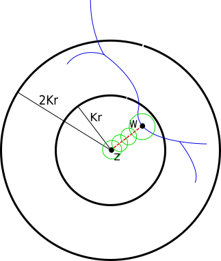
Figure 1. The interval $[z,w]$ covered by $N_{1}$ smaller disks

Since $D_{Kr}(w)\subset D_{2Kr}(z)$ it follows that $D_{Kr}(w)\subset\Omega$. Hence the disk $D_{\frac{r}{2}}(w)$ satisfies the conditions of the previously discussed case, and we obtain the estimates

$$\mathrm{diam}_{\Omega}D^{-i}_{\frac{r}{2}}(w)\leq N_{0}(2K)\cdot C(\frac{1}{2},\mathrm{deg}_{\mathrm{crit}}).$$

The interval $[z,w]$ can be covered by the disk $D_{\frac{r}{2}}(w)$ and a bounded number of disks $D_{s_{1}}(w_{1}),\ldots,D_{s_{N_{1}}}(w_{N_{1}})$ satisfying $D_{Ks_{\nu}}(w_{\nu})\subset U^{n}$ for a universal constant $N_{1}\in\mathbb{N}$. Thus the disks $D_{s_{\nu}}(w_{\nu})$ satisfy the conditions of Lemma 2.10, and it follows that

$$\mathrm{diam}_{\Omega}D^{-i}_{s_{\nu}}(w_{\nu})\leq\mathrm{diam}_{\mathrm{max}}.$$

Thus, we obtain a bound from above on the hyperbolic distance of each $D^{-i}_{r}(z)$ to $\partial U^{n-i}$. By choosing $\Omega$ sufficiently thin, the bounds on the hyperbolic distance to the boundary gives arbitrarily small bounds on the Euclidean distance to the boundary, which in turn means that hyperbolic diameter estimates give arbitrarily small bounds on the Euclidean diameters of the disks $D^{-i}_{r_{k}}(z_{k})$. We can conclude the argument by using the same induction on $i$ used in the previously discussed cases. ∎

2.4. Consequences

The obtained degree and diameter estimates imply a number of consequences. The first is the non-existence of wandering domains.

Lemma 2.11.

There are no wandering Fatou components.

Proof.

Suppose $U$ is a wandering Fatou component. We can construct the domain $\Omega$ as above sufficiently thin so that the Poincaré diameter of $U$ can be made arbitrarily large. In particular, we can find a relatively compact $K\subset U$ whose Poincaré diameter in $\Omega$ is strictly larger than $\mathrm{diam}_{\mathrm{max}}$. Let $n_{j}$ such that $f^{n_{j}}(K)$ converges to a point $p\in J$. Without loss of generality we may assume that $p$ does not lie in a parabolic cycle. Let $D_{r}(p)$ be such that $D_{2r}(p)\subset\Omega$. Then $f^{n_{j}}(K)\subset D_{r}(p)$ for sufficiently large $j$, which by Proposition 2.1 implies that $\mathrm{diam}(K)<\mathrm{diam}_{\mathrm{max}}$, giving a contradiction. ∎

Lacking wandering domains the proof of Proposition 2.1 becomes considerably simpler. An immediate consequence is the following.

Corollary 2.12.

The constant $\mathrm{deg}_{\mathrm{crit}}$ can be taken equal to $1$, and the constant $M$ equal to $2$.

Proposition 2.13.

Let $z\in J$ not be contained in a parabolic cycle, choose $r>0$ so that $D_{r}(z)\subset D_{2r}(z)\subset\Omega$, and let $V^{1},V^{2},\ldots$ be such that $f(V^{1})=D_{r}$ and $f(V^{n+1})=V^{n}$. Then

$$\mathrm{diam}_{\Omega}V^{n}\rightarrow 0.$$

Proof.

By Corollary 2.12 the maps $f^{n}:V^{n}\rightarrow D_{r}$ are all univalent, hence we can consider the inverse branches $(f^{n})^{-1}:D_{r}\rightarrow V^{n}$. These inverse branches form a bounded, and thus normal, family of holomorphic maps. Let $h$ be a limit map. Since $z\in J$ and $J$ is invariant, the image $h(D_{r})$ must contain a point $q$ in $J$. But since any neighborhood of $q$ contains points in the basin of infinity, $h(D_{r})$ cannot contain an open neighborhood of $q$, and hence $h$ is constant. ∎

The non-existence of rotation domains is an immediate consequence.

Corollary 2.14.

The polynomial $f$ does not have any Siegel disks.

Corollary 2.15.

If $f$ does not have any parabolic cycles then $f$ is hyperbolic.

Proof.

When $f$ lacks parabolic cycles the set $J$ is contained in $\Omega$. Since $J$ is compact it follows from Proposition 2.13 that there exist $N\in\mathbb{N}$ and $r>0$ such for any $z\in D$ and any connected component $V^{N}$ of $(f^{n})^{-1}(D_{r}(z))$ the Euclidean diameter of $V^{N}$ is less than $r/2$. The Schwartz Lemma therefore implies that $|(f^{N})^{\prime}|\geq 2$ on $J$. ∎

Corollary 2.16.

The polynomial $f$ lies on the boundary of the hyperbolicity locus.

Proof.

By [DH85] the number of parabolic cycles is bounded by the degree of $f$. It follows that we can perturb the parameters $f$ slightly in a direction where $J$ changes continuously, and so that all parabolic cycles split into repelling and attracting cycles. If the perturbation is sufficiently small then there are still no critical points on $J$, while the parabolic cycles have disappeared. Hence by the previous Corollary the perturbed function is hyperbolic. ∎

We note that the bound on the number of parabolic cycles in terms of the degree is not needed if one allows perturbations into the infinite dimensional space of polynomial like maps.

3. Hénon maps: Background and preliminaries

Recall from [FM89] that the dynamical behavior of a polynomial automorphism of $\mathbb{C}^{2}$ is either dynamically trivial, or the automorphism is conjugate to a finite composition of maps of the form

$$(x,y)\mapsto(p(x)+b\cdot y,x),$$

where $p$ is a polynomial of degree at least $2$ and $b\neq 0$. We will refer to such compositions as Hénon maps. Given $R>0$ we define the following sets.

$$\Delta^{2}_{R} :=\{(x,y):|x|,|y|<R\},$$

$$V^{+} :=\{(x,y):|x|\geq\max(R,|y|)\},\;\;\mathrm{and}$$

$$V^{-} :=\{(x,y):|y|\geq\max(R,|x|)\}$$

By choosing $R$ sufficiently large we can make sure that $f(V^{+})\subset V^{+}$, $f^{-1}(V^{-})\subset V^{-}$ and $f(\Delta^{2}_{R})\subset\Delta^{2}_{R}\cup V^{+}$. One can also guarantee that if $(x_{0},y_{0})\in V^{+}$ and $(x_{1},y_{1})=f(x_{0},y_{0})$ then $|x_{1}|>2|x_{2}|$. Similarly one obtains $|y_{-1}|>2|y_{0}|$ for $(x_{0},y_{0})\in V^{-}$. It follows that every orbit that lands in $V^{+}$ must escape to infinity, and every orbit that does not converge to infinity must eventually land in $\Delta^{2}_{R}$ in a finite number of steps.

We write $K^{+}$ for the set with bounded forward orbits, $K^{-}$ for the set with bounded backward orbits, and $K=K^{+}\cap K^{-}$. As usual we define the forward and backward Julia sets as $J^{\pm}=\partial K^{\pm}$, and the Julia set as $J=J^{+}\cap J^{-}$. Let us recall the existence of the Green’s currents $T^{+}$ and $T^{-}$, supported on $J^{+}$ and $J^{-}$, and the equilibrium measure $\mu=T^{+}\wedge T^{-}$, whose support $J^{\star}$ is contained in $J$. Whether $J^{*}$ always equals $J$ is one of the main open questions in the area, and was previously only known for hyperbolic Hénon maps [BS91a].

3.1. Wiman Theorem and Substantially dissipative Hénon maps

Recall that a subharmonic function $g:\mathbb{C}\rightarrow\mathbb{R}$ is said to have order of growth at most $\rho$ if

$$g(\zeta)=O(|z|^{\rho})\quad{\mathrm{as}}\quad\zeta\rightarrow\infty.$$

Given $E\in\mathbb{R}$, let us call the set $\{g<E\}$ subpotential (of level $E$), and its components subpotential components.

Theorem 3.1 (Wiman).

Let $g$ be a non-constant subharmonic function with order of growth strictly less than $\frac{1}{2}$. Then subpotential components of any level $E$ are bounded.

Let us describe how it was used in the setting of Hénon maps in recent works of the first author and Dujardin [DL15], and in [LP14]. Suppose that $p\in\mathbb{C}^{2}$ is a hyperbolic fixed point, and let $W^{s}(p)$ be its stable manifold, corresponding to the stable eigenvalue $\lambda$. Then there exists a linearization map $\varphi:\mathbb{C}\rightarrow W^{s}(p)$ satisfying $\varphi(\lambda\cdot\zeta)=f(\varphi(\zeta))$. As usual we let $G^{\pm}$ be the plurisubharmonic functions defined by

$$G^{\pm}(z)=\lim_{n\rightarrow\infty}\frac{1}{(\deg f)^{n}}\cdot\log^{+}\|f^{\pm n}(z)\|.$$

We have the functional equations

$$G^{\pm}(f(z))=(\mathrm{deg}f)^{\pm 1}\cdot G^{\pm}(z).$$

Combining the functional equations for $G^{-}$ and $\phi$ we obtain that the non-constant subharmonic function $g=G^{-}\circ\varphi$ satisfies

$$g(\lambda\cdot\zeta)=G^{-}\circ f\circ\varphi(\zeta)=\frac{1}{\deg f}g(\zeta).$$

Note that $|\lambda|<|\mathrm{Jac}f|$. Hence under the assumption that $|\mathrm{Jac}f|<\frac{1}{\mathrm{deg}f^{2}}$ it follows that $g$ is a subharmonic function of growth strictly less than $\frac{1}{2}$, and therefore according to Wiman’s Theorem all its subpotential components are bounded.

Let us point out that the above discussion also holds when $p$ is a neutral fixed point, i.e. having one neutral and one attracting multiplier. One considers the strong stable manifold with corresponding eigen value $\lambda$, satisfying $|\lambda|=|\mathrm{Jac}f|$. The subharmonic function $g$ still has order of growth strictly less than $\frac{1}{2}$. The idea can also be applied when $p$ is not a periodic point but lies in a invariant hyperbolic set, or under the assumption of a dominated splitting, which will be discussed in the next section.

A particular consequence of Wiman’s Theorem is that all connected components of intersections of (strong) stable manifolds with $\Delta^{2}_{R}$ are bounded in the linearization coordinates. By the Maximum Principle they are also simply connected, hence they are disks. The filtration property of Hénon maps tells us that every connected component of the intersection of a stable manifold with $\Delta^{2}_{R}$ is actually a branched cover over the vertical disk $\Delta_{w}(R)$. This will be used heavily in what follows.

3.2. Classification of periodic components

3.2.1. Ordinary components

We recall the classification of periodic Fatou components $U$ from [LP14], building upon results of Bedford and Smillie [BS91b]. For a dissipative Hénon map $f$, there exist three types of ordinary invariant Fatou components $U$:

1. Attracting basin: All orbits in $U$ converge to an attracting fixed point $p\in U$. Moreover, $U$ is a Fatou-Bieberbach domain (i.e., it is biholomorphically equivalent to $\mathbb{C}^{2}$).

2. Rotation basin: All orbits in $U$ converge to a properly embedded Riemann surface $\Sigma\subset U$, which is invariant under $f$ and biholomorphically equivalent to either an annulus or the unit disk. The biholomorphism from $\Sigma$ to an annulus or disk can be chosen so that it conjugates the action of $f|_{\Sigma}$ to an irrational rotation. The stable manifolds through points in $\Sigma$ are all embedded complex lines, and the domain $U$ is biholomorphically equivalent to $\Sigma\times\mathbb{C}$.

3. Parabolic basin: All orbits in $U$ converge to a parabolic fixed point $p\in\partial U$ with the neutral eigenvalue equal to $1$. Moreover, $U$ is a Fatou-Bieberbach domain.

In the literature a periodic point whose multipliers $\lambda_{1}$ and $\lambda_{2}$ satisfying $|\lambda_{1}|<1$ and $\lambda_{2}=1$ may be called either semi-parabolic or semi-attracting, depending on context. Since we are working with dissipative Hénon maps, where there is always at least one attracting multiplier, we chose to refer to these points as parabolic, and we use analogues terminology for Fatou components. Similarly, we will call a periodic point with one neutral multiplier neutral.

In each case, we let $A=A_{U}$ be the attractor of the corresponding component (i.e., the attracting or parabolic point $p$, or the rotational curve $\Sigma$).

Along with global Fatou components $U$, we will consider semi-local ones, which are components $U^{i}$ of the intersection $U\cap\Delta^{2}_{R}$. (Usually there are infinitely many of them.) Each $U^{i}$ is mapped under $f$ into some component $U^{j}$, $j=j(i)$, with “vertical” boundary $\partial U^{i}\cap\Delta^{2}_{R}$ being mapped into the vertical boundary of $U^{j}$, but the correspondence $i\mapsto j(i)$ is not in general injective. This dynamical tree of semi-local components resembles closely the one-dimensional picture. In particular, cycles of ordinary semi-local components can be viewed as the immediate basins of the corresponding attractors $A_{U}$.

3.2.2. Absorbing domains

Given a compact subset $Q\subset U$, let us say that an invariant domain $D\subset U$ is $Q$-absorbing if there exist a moment $n\in\mathbb{N}$ such that $f^{n}(Q)\subset D$. If this happens for any $Q$ (with $n$ depending on $Q$) then $D$ is called absorbing.

For instance, in the attracting case, any forward invariant neighborhood of the attracting point is absorbing. In the parabolic case, there exists an arbitrary small absorbing “attracting petal” $P\subset U$ with $\partial P\cap\partial U=\{p\}$ (see [BSU17]). To construct a $Q$-absorbing domain in the rotation case, take a sufficiently large invariant subdomain $\Sigma^{\prime}\subset\Sigma$ compactly contained in $\Sigma$ and let

$$D=\bigcup_{z\in\Sigma^{\prime}}W_{{\operatorname{loc}}}^{s}(z).$$

This implies:

Lemma 3.2.

Let $f$ be a dissipative Hénon map, and let $U$ be an ordinary invariant Fatou component with an attractor $A$. Then any compact set $Q\subset U$ is contained in a forward invariant domain $W\subset U$ such that $\overline{W}\cap\partial U\subset A$. (In particular, $W$ is relatively compactly contained in $U$ in the attracting or rotation cases.)

Let us say that a subset $\Omega\subset\Delta^{2}_{R}$ is relatively backward invariant if

$$f^{-1}(\Omega)\cap\Delta^{2}_{R}\subset\Omega.$$

Corollary 3.3.

Given any compact set $Q$ contained in the union of periodic Fatou components, there exists an open and relatively backward invariant subset $\Omega$ of $\Delta^{2}_{R}$ containing

$$\Delta^{2}_{R}\cap(\mathrm{wandering\ components}\cup J^{+}\setminus\overline{\{{\mathrm{parabolic\ cycles}}\}})$$

and avoiding $Q$.

Proof.

There exist only finitely many periodic Fatou components $U^{i}$ intersecting $Q$. For each of them, let $W_{i}$ be the neighborhood of $(Q\cap U^{i})$ from Lemma 3.2. Note that $J^{+}\cap(\bigcup\overline{W_{i}})$ is contained in a finite number of parabolic cycles. Take now a small ${\varepsilon}>0$ and let

$$\Omega=\Delta^{2}_{R}\cap\{G^{+}<{\varepsilon}\}\setminus(\bigcup\overline{W_{i}}).$$

∎

3.2.3. Substantially dissipative maps

Theorem 3.4 ([LP14]).

For a substantially dissipative Hénon map, any periodic Fatou component is ordinary.

Remark 3.5.

In fact, for Hénon maps with dominated splitting, this classification holds without assuming that dissipation is substantial, see Proposition 4.1 below.

4. Dominated splitting

4.0.1. Definition

We say that a Hénon map $f$ admits a dominated splitting if there is an invariant splitting of the tangent bundle on $J=J^{+}\cap J^{-}$

(1) $$T_{J}(\mathbb{C}^{2})=E^{s}\oplus E^{c}$$

with constants $0<\rho<1$ and $C>0$ such that for every $p\in J$ and any unit vectors $v\in E^{s}_{p}$ and $w\in E^{c}_{p}$ one has

$$\frac{\|df^{n}v\|}{\|df^{n}w\|}<C\cdot\rho^{n}.$$

From now on we will assume that $f$ is dissipative, from which it immediately follows that $E^{s}$ is stable. We cannot conclude that $E^{c}$ is unstable, though.

4.0.2. Cone fields

Let $p\in J$ and let $v\subset E^{s}_{p}$ have unit length. Given $0<\alpha<1$ we can define the cone

$$C_{p}^{s}(\alpha):=\{w\in T_{p}(\mathbb{C}^{2}):|<w,v>|\geq\alpha\|w\|\}.$$

It follows from the dominated splitting that we can choose $\alpha$ continuously, depending on $p\in J$, so that

$$dfC_{p}^{s}(\alpha(p))\supset C_{f(p)}^{s}(r\cdot\alpha(f(p)))$$

for some $r<1$ which can be chosen independently of $p\in J$. We refer to the collection of these cones as the (backward) invariant vertical cone field on $J$.

Since both $E^{s}_{p}$ and $\alpha$ vary continuously with $p$, and the set $J$ is closed, we can extend the vertical cone field continuously to $\Delta^{2}_{R}$. It follows automatically that the extension of the cone field to $\Delta^{2}_{R}$ is backward invariant for points lying in a sufficiently small neighborhood $\mathcal{N}(J)$.

Note that all accumulation points of the forward orbit of a point in $J^{+}$ must lie in $K^{-}=J^{-}$, and therefore in $J=J^{+}\cap J^{-}$. Writing $J^{+}_{R}=J^{+}\cap\Delta^{2}_{R}$ as before, it follows from compactness that there exists an $N\in\mathbb{N}$ such that $f^{n}(J^{+}_{R})\subset\mathcal{N}(J)$ for all $n\geq N$. Thus we can pull back the vertical cone field to obtain a backwards invariant cone field on a neighborhood of $J^{+}_{R}$. We will denote this neighborhood by $\mathcal{N}(J^{+}_{R})$, and refer to it as the region of dominated splitting.

4.0.3. Strong stable manifolds

Let us consider the following completely invariant set:

(2) $${\mathcal{V}}^{+}:=\{p:\ \exists\ n_{0}=n_{0}(p)\ f^{n}p\in{\mathcal{N}}(J)\ {\mathrm{f}or}\ n\geq n_{0}\}.$$

Let $U(p)$ be a small ball centered at $p$. For $p\in{\mathcal{V}}^{+}$, consider a straight complex line through $f^{n}(p)$ whose tangent space at $f^{n}(p)$ is contained in the vertical cone, and pull back this line by $f^{n}$, keeping only the connected component through $p$ in the neighborhood $U(p)$. By the standard graph transform method, this sequence of holomorphic disks converges to a complex submanifold $W^{s}_{\operatorname{loc}}(p)$, the so-called local strong stable manifold through $p$. By pulling back the local stable manifolds through $f^{n}(p)$ by $f^{-n}$ we obtain in the limit the global strong stable manifold through $p$, denoted by $W^{s}(p)$. In line with our earlier introduced notation we will write $W^{s}_{R}(p)$ for the connected component of $W^{s}(p)\cap\Delta^{2}_{R}$ that contains $p$, and refer to it as a semi-local stable manifold.

We will refer to the collection of these semi-local strong stable manifolds as the (semi-local) dynamical vertical lamination.

For $p\in{\mathcal{V}}^{+}$, we let $E^{s}_{p}$ be the tangent line to $W^{s}(p)$, which can be also constructed directly as

$$E^{s}_{p}=\bigcap_{n\geq 0}df^{-n}C^{s}_{f^{n}p}(\alpha).$$

The lines $E^{s}_{p}$ form the stable line field over ${\mathcal{V}}^{+}$, extending the initial stable line (1) field over $J$.

Similarly to ${\mathcal{V}}^{+}$ we can consider

(3) $${\mathcal{V}}^{-}:=\{p:\ \exists\ n_{0}=n_{0}(p)\ f^{-n}p\in{\mathcal{N}}(J)\ {\mathrm{f}or}\ n\geq n_{0}\}.$$

For $p\in{\mathcal{V}}^{-}$ we cannot guarantee the existence of a horizontal center manifold, but there does exist a unique central line field, i.e. a tangent subspace whose pullback under $f^{n}$ is contained in the horizontal cone field for all $n\geq n_{0}$. For points $p\in{\mathcal{V}}^{+}\cap{\mathcal{V}}^{-}$ we can consider both the vertical and the central line field. Tangencies between those two line fields play the role of critical orbits. By the dominated splitting these can only occur for orbits that leave and come back to the domain of dominated splitting. A major part of this paper is aimed at obtaining a better understanding of such tangencies.

4.0.4. Linearization coordinates

The global strong stable manifolds $W^{s}(p)$ of points $p$ in the dynamical vertical lamination can be uniformized as follows. Denote by $\pi_{p}:W^{s}(p)\rightarrow T_{p}(W^{s}(p))$ the projection to the tangent plane. The projection is locally a biholomorphism, as local stable manifolds are graphs over the tangent plane. The size of the local stable manifolds can be taken uniform over all $p$ in the dynamical vertical lamination. Define $\varphi_{p}:W^{s}(p)\rightarrow T_{p}(W^{s}(p))$ by

$$\varphi_{p}=\lim_{n\rightarrow\infty}[Df^{n}(p)]^{-1}\circ\pi_{f^{n}(p)}\circ f^{n}.$$

Identifying the tangent plane with $\mathbb{C}$ we can view $\varphi_{p}$ as a biholomorphic map from $W^{s}(p)$ to $\mathbb{C}$. This identification is canonical up to a choice of argument. The identifications can locally be chosen to vary continuously with $p$. As the tangent planes to the dynamical vertical lamination vary continuously with $p$, and the above convergence to $\varphi_{p}$ is uniform over $p$ in the dynamical vertical lamination, one can locally obtain a continuous family of linearization maps $\varphi:W^{s}(p)\rightarrow\mathbb{C}$.

The composition of the Green’s function $G^{-}$ with the linearization map gives a subharmonic function on the $\mathbb{C}$-coordinates of $W^{s}(p)$, which, provided the neighborhood $\mathcal{N}_{R}(J^{+})$ is made sufficiently thin, has order of growth strictly less than $\frac{1}{2}$. Hence for each point $p\in\mathcal{N}_{R}(J^{+})$ the local stable manifold $W^{s}_{R}(p)$ is a properly embedded disk in $\Delta^{2}_{R}$, with the projection to the second coordinate giving branched covers of uniformly bounded degrees.

4.0.5. Fatou components

While the substantial dissipativity assumption plays an important role in the current paper, the bound on the Jacobian in terms of the degree is not needed for the classification of periodic Fatou components in the dominated splitting setting:

Proposition 4.1.

For a dissipative Hénon map with dominated splitting, any periodic Fatou component is an ordinary component.

Proof.

In [LP14] the assumption that the Hénon map is substantially dissipative plays a role in only an isolated part of the proof, namely to prove the uniqueness of limit sets on non-recurrent Fatou components. We note that in order to prove this uniqueness, one does not need to assume substantial dissipativity for Hénon maps admitting a dominated splitting. Recall that the only point in the proof where substantial dissipativity is used, is to rule out a one-dimensional limit set $\Sigma$ contained in the strong stable manifold of a hyperbolic or neutral fixed point. Suppose that there exists a dominated splitting near $J$, and that such a $\Sigma$ does exist. As was pointed out in [LP14], the restriction of $\{f^{n}\}$ to $\Sigma$ is a normal family. Recall also that $\Sigma$ must lie in $J$, hence through each point $q\in\Sigma$ there exists a strong stable manifold $W^{s}(q)$. If $\Sigma$ is transverse to the stable field $\{E^{s}\}$ at some point $q\in\Sigma$, then the union of the stable manifolds contains an open neighborhood of $q$, on which the family of iterates is necessarily a normal family. This gives a contradiction with $\Sigma\subset J$. On the other hand, if $\Sigma$ is everywhere tangent to the stable field, then for any $q\in\Sigma$, it is a domain in the stable manifold $W^{s}(q)$. Being backward invariant, $\Sigma$ must coincide with $W^{s}(q)$. However, $W^{s}(q)$ is conformally equivalent to $\mathbb{C}$, while $\Sigma$ cannot, giving a contradiction. ∎

It is a priori not clear that there are only finitely many periodic components. In the substantially dissipative case finiteness is a consequence of our main result.

4.0.6. Rates

We will show now that the rate of contraction on the central line bundle is subexponential.

Lemma 4.2.

Given any $r_{1}<1$ there exists a $C>0$ such that for any $p\in J$ and any unit vector $w\in E^{c}_{p}$ we have

$$\|df^{n}w\|>\frac{1}{C}\cdot{r_{1}}^{n}.$$

Proof.

Let us for the purpose of a contradiction suppose that for some $r_{1}<1$ there exist for arbitrarily large $n\in\mathbb{N}$ unit vectors $w_{n}\in E^{c}$ with

$$\|df^{n}w_{n}\|<r_{1}^{n}.$$

Let $r_{1}<r_{2}<1$. Then there exists an $\epsilon>0$ and for every $n\in\mathbb{N}$ an integer $k\in\{0,1,\ldots n-1\}$ such that

$$\|df^{j}(df^{k}w_{n})\|<r_{2}^{j}\cdot\|df^{k}w_{n}\|$$

for $j\leq\epsilon\cdot n$. It follows that for every $m\in\mathbb{N}$ there exists a unit vector $u_{m}\in E^{c}$ for which

$$\|df^{j}u_{m}\|<r_{2}^{j}$$

for $j=0,\ldots m$. Here $u_{m}$ can be chosen a multiple of a vector $df^{k}w_{n}$.

Since the set of unit vectors in $E^{c}$ is compact, there exists an accumulation point $w\in E^{c}$ of the sequence $(u_{m})$. Let $p\in J$ be such that $w\in E^{c}_{p}$. By continuity of the differential $df$ it follows that

$$\|df^{j}w\|\leq r_{2}^{j}$$

for all $j\in\mathbb{N}$. Since $T_{p}(\mathbb{C}^{2})=E_{p}^{s}\oplus E_{p}^{c}$, and by the definition of the dominated splitting, there exists a $C>0$ such that

$$\|Df^{j}(z_{0})\|<C\cdot r_{2}^{j}$$

for all $j\in\mathbb{N}$. Here we have used that there is a uniform bound from below on the angle between the vertical and horizontal tangent spaces.

Let $\xi>1$ be sufficiently small such that $\xi\cdot r_{2}<1$. By compactness of $\Delta^{2}_{R}$ there exists a $\rho>0$ such that if $x,y\in\Delta^{2}_{R}$ with $\|x-y\|<\rho$ then

$$\|f(x)-f(y)\|\leq\xi\cdot\|Df(x)\|\cdot\|x-y\|.$$

Let $z\in\Delta^{2}_{R}$ be such that $\|z-p\|<\frac{\rho}{C}$. Then it follows by induction on $n$ that

$$\|f^{n}(z)-f^{n}(p)\|\leq\rho(\xi\cdot r_{2})^{n}$$

for every $n\in\mathbb{N}$. Hence there is a neighborhood $U$ of $p$ such that

$$\|f^{n}(z)-f^{n}(p)\|\rightarrow 0,$$

uniformly over all $z\in U$. But then $\{f^{n}\}_{n\in\mathbb{N}}$ is a normal family on $U$, which contradicts the fact that $p\in J^{+}$. ∎

It follows that the exponential rate of contraction on the stable subbundle is at least $\delta$.

Lemma 4.3.

Given any $r>|\delta|$ we can find $C>0$ such that for any unit vector $v\in E^{s}$ we have

$$\|df^{n}v\|<C\cdot r^{n}.$$

Proof.

Write $v\in E^{s}_{p}$, and let $w\in E^{c}_{p}$ be a unit vector. The inequality follows immediately from Lemma 4.2 and the fact that

$$\|df^{n}v\|\cdot\|df^{n}w\|\leq C_{1}|\delta|^{n},$$

where the constant $C_{1}$ depends on minimal angle between the spaces $E^{s}$ and $E^{c}$. ∎

5. Dynamical lamination and its extensions

5.1. Dynamical lamination

Now let us assume that the map $f$ is substantially dissipative. Then the rate $r$ in Lemma 4.3 can be assumed to be strictly smaller than $1/d^{2}$.

It follows that for any point $p\in J$, the composition $G^{-}\circ\varphi_{p}$ is a subharmonic function of order bounded by $\rho<\frac{1}{2}$, so the Wiman Theorem can be applied. It implies that $W^{s}_{R}(p)$ is an embedded holomorphic disk, and that the projection to the second coordinate $\pi_{2}:W^{s}_{R}(p)\rightarrow\Delta_{R}$ gives a branched covering of finite degree.

Lemma 5.1.

The degrees of the branched coverings $\pi_{2}:W^{s}_{R}(p)\rightarrow\Delta_{R}$ are uniformly bounded, and

$$J^{+}_{R}=\bigcup_{p\in J}W^{s}_{R}(p).$$

Proof.

Let $q\in J^{+}_{R}$. Note that the sets

$$V_{n}(q)=\{(x,y)\in W^{s}_{R}(q):f^{-n}(x,y)\in\Delta^{2}_{R}\}$$

form a nested sequence of non-empty compact sets, so they have a non-empty intersection. Hence each $W^{s}_{R}(q)$ intersects $K^{-}=J^{-}$. Therefore we have

$$J^{+}_{R}=\bigcup_{p\in J}W^{s}_{R}(p).$$

Note that the degree of $W^{s}_{R}(p)$ depends lower semi-continuously on $p$; the degree may drop at semi-local stable manifolds tangent to the boundary of $\Delta^{2}_{R}$. However, when we consider the restriction of such a stable manifold to a strictly larger bidisk $\Delta^{2}_{R^{\prime}}$, its degree, which is still finite, is at least as large as the degree of sufficiently nearby stable manifolds restricted to the smaller bidisk $\Delta^{2}_{R}$.

To argue that the degrees of the branched coverings are uniformly bounded, suppose for the purpose of a contradiction that there is a sequence $(W^{s}_{R}(p_{j}))$ for which the degrees converge to infinity. Without loss of generality we may assume that the sequence $(p_{j})$ converges to a point $p\in J^{+}_{R}$. Let $R^{\prime}>R$. Then for $j$ sufficiently large the degree of $W^{s}_{R}(p_{j})$ is bounded by the degree of $W^{s}_{R^{\prime}}(p)$, which gives a contradiction. ∎

We will refer to the lamination on $J^{+}\cap\Delta^{2}_{R}$ given by these local strong stable manifolds as the (semi-local) dynamical lamination. In what follows we will extend this lamination, in a non-dynamical way, to a larger subset of $\Delta^{2}_{R}$.

5.2. Local and global extensions of the vertical lamination

We note that the dynamical vertical lamination discussed previously consists of local leaves $L_{R}(a)$ that are connected components of global leaves $L(a)$ intersected with $\Delta^{2}_{R}$. These leaves all have natural linearization parametrizations that vary continuously with the base point $a$.

Let us recall the $\lambda$-lemma, in this version due to Slodkowski [Sl91].

Lemma 5.2.

Let $A\subset\hat{\mathbb{C}}$. Any holomorphic motion $f:\mathbb{D}\times A\rightarrow\hat{\mathbb{C}}$ of $A$ over $\mathbb{D}$ extends to a holomorphic motion $\mathbb{D}\times\hat{\mathbb{C}}\mapsto\hat{\mathbb{C}}$ of $\hat{\mathbb{C}}$ over $\mathbb{D}$.

Let $L_{R}(a)$ be a dynamical leaf, with a linearization map $\varphi_{a}:\mathbb{C}\rightarrow L(a)$. Recall that by the assumption that $f$ is substantially dissipative we have that $L_{R}(a)=\varphi_{a}(D)$, for some bounded simply connected set $D\subset\mathbb{C}$. Let $D$ be compactly contained in a slightly larger simply connected set $D^{\prime}$, and let $\xi:\mathbb{D}\rightarrow D^{\prime}$ be the Riemann mapping. Define $\psi_{a}=\varphi_{a}\circ\xi:\mathbb{D}\rightarrow L_{R}(a)$. Then there exists a biholomorphic map $\Psi$ from $\Delta_{\epsilon}\times\mathbb{D}\rightarrow\mathbb{C}^{2}$ with $\Psi(\zeta,0)=\psi_{a}(\zeta)$, mapping to a tubular neighborhood of the “core” $L_{R}(a)$. Consider all dynamical leaves that intersect a small neighborhood $\Psi(\Delta_{\delta}\times\mathbb{D}\rightarrow\mathbb{C}^{2})$, where $\delta$ is chosen sufficiently small so that these dynamical leaves are completely contained in $\Psi(\Delta_{\epsilon}\times\mathbb{D}\rightarrow\mathbb{C}^{2})$. If $\epsilon$ is sufficiently small then the inverse images under $\Psi$ of these leaves form a collection of pairwise disjoint “dynamical” graphs over $\mathbb{D}$ in $\Delta_{\epsilon}\times\mathbb{D}$, thus giving a holomorphic motion of a set $A\subset\Delta_{\epsilon}$.

By the $\lambda$-lemma the motion extends to a holomorphic motion over $\Delta_{\epsilon}$. The graphs over $\mathbb{D}$ that are completely contained in $\Delta_{\epsilon}\times\mathbb{D}$ can be mapped back by $\Psi$. By restricting to a slightly smaller vertical disk $D_{1-\eta}$, we can guarantee that all graphs that intersect a sufficiently small neighborhood of the core $\{0\}\times\mathbb{D}_{1-\eta}$ are completely contained in $\Delta_{\delta}\times D_{1-\eta}$, and can therefore be mapped back to $\mathbb{C}^{2}$ by $\Psi$. We obtain a collection of pairwise disjoint ”graphs” over $L_{R}(a)$, filling a neighborhood and all remaining in the neighborhood sufficiently close to $L_{R}(a)$. Moreover, by construction the newly constructed graphs cannot intersect any dynamical graphs.

We will refer to such an extension as a flow box, and to the leaves as vertical. Note that the dynamical leaves were globally defined, while the new leaves in the flowboxes are only defined in $\Delta^{2}_{R}$.

By compactness the Euclidean radii of the tubular neighborhoods of the dynamical leaves can be chosen uniformly, and hence the dynamical vertical lamination is contained in a finite number of flow boxes. One could apply the $\lambda$-lemma to each of these, but a priori there is no reason why new leaves coming from different flow boxes should not intersect transversely. The main result in this section is Proposition 5.8, where a single extension to a neighborhood of the dynamical vertical lamination is constructed. Let us give an outline of the argument before going into details.

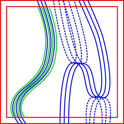
Figure 2. Local extension of the lamination on slightly smaller bidisk

The extension of the lamination will be constructed by applying the $\lambda$-lemma to a finite number of tubular neighborhoods, each time taking into account the leaves that have been considered in previous steps.

A difficulty is that the leaves that we construct in a local extension are not global, they only are defined in some the tubular neighborhood. In particular, even if we can guarantee that all new leaves, are graphs over the core of other tubular neighborhoods they intersect, they may not be graphs over the entire core, see Figure 3(a). We can deal with this by starting with a strictly larger bidisk $\Delta^{2}_{R^{\prime}}$, and reducing the radius $R^{\prime}$ after each local extension by twice the radius of the tubular neighborhood. The goal is therefore to reduce the radius by at most the difference $R^{\prime}-R$ we start with.

Starting with an even larger constant $R^{\prime}$ is not of help, as that would affect the size and geometry of the flowboxes. Just reducing the radii of the flow boxes seems useless as well, as that would increase the number of flow boxes needed. The solution is to carry out the $\lambda$-lemma on large numbers of pairwise disjoint flow boxes simultaneously. By a covering lemma a la Besicovitch it follows that we can finish the process in a number of steps $N$ that is independent of the radii of the flow boxes. By starting with a slightly larger bidisk $\Delta^{2}_{R^{\prime}}$ and choosing the radii $\epsilon$ so that $N\cdot 2\times\epsilon<R^{\prime}-R$ we will obtain the desired extension.

The version of Besicovitch Covering Theorem that we will use relies on the fact that the dynamical vertical lamination is Lipschitz, which follows from the following:

Lemma 5.3.

The holonomy maps of the dynamical vertical lamination are $C^{1+\epsilon}$ smooth.

Proof.

The analogous statement in the uniformly hyperbolic case was proved in [L99], with a similar proof. It is sufficient to prove that under the holonomy maps induced by the dynamical vertical lamination, the dilatation of images of small disks of radius $r>0$ is $1+r^{\epsilon}$, for some $\epsilon>0$.

We consider holonomy between horizontal transversals through two points $z,w$ with $w\in W^{s}_{loc}(z)$. Let $\eta>0$ be such that any horizontal disk through any point $f^{n}(z)$ or $f^{n}(w)$ of radius at most $\eta$ is a graph over the horizontal tangent line.

Let $D(z)$ and $D(w)$ be horizontal transversal disks, let $0<r<\eta$, and let $\Delta_{r}(z)\subset D(z)$ be a graph over the disk of radius $r$. We choose $n\in\mathbb{N}$ be so that

$$\|df^{n}|_{E^{s}_{z}}\|\sim\frac{r}{\eta}.$$

Note that

$$\|df^{n}|_{E^{c}_{z}}\|\cdot\|df^{n}|_{E^{s}_{z}}\|\sim|\mathrm{Jac}(f)|^{n},$$

and thus decreases exponentially fast. It follows that for $r$ sufficiently small, the disks $\Delta^{n}_{r}(z)=f^{n}\Delta_{r}(z)$ have size $<\eta$, so they are graphs over the horizontal tangent line at $f^{n}(z)$. Hence the composition of $f^{n}:\Delta_{r}(z)\rightarrow\Delta^{n}_{r}(z)$ with the respective projections to and from the respective horizontal tangent lines at $z$ and $f^{n}(z)$ produces a univalent function.

Consider the disks $\Delta_{r^{2}}(z)\subset\Delta_{r}(z)$. By the Koebe Distortion Theorem, the dilatation of $\Delta^{n}_{r^{2}}(z)$ is bounded by $1+O(r)$. By our choice of $n$ it follows that $\|z^{n}-w^{n}\|$ is of order $r$. Hence the holonomy from $\Delta^{n}_{r}(z)$ to its image $\Delta^{n}_{r}(w)$ is quasiconformal of order $r$, and the dilatation of $\Delta^{n}_{r^{2}}(w)$ is bounded by $1+O(r)$.

The modulus $-\log(r)$ of the annulus $\Delta_{r}(z)\setminus\Delta_{r^{2}}(z)$ is preserved under conformal maps, hence $\mathrm{Mod}(\Delta^{n}_{r}(z)\setminus\Delta^{n}_{r^{2}}(z))=-\log(r)$. Since the distance between the disks $\Delta_{r}(z)$ and $\Delta_{r}(w)$ is of order $r$, the holonomy map from one to the other changes the modulus of the respective annuli by at most a factor of order $1-r$, hence

$$\mathrm{Mod}(\Delta^{n}_{r}(w)\setminus\Delta^{n}_{r^{2}}(w))=\geq((1-O(r))\cdot\log(\frac{1}{r}))=\geq\log(\frac{1}{r^{1-O(r)}}).$$

Therefore, we can again apply the Koebe Distortion Theorem to conformal map $f^{-n}:\Delta^{n}_{r}(w)\rightarrow\Delta_{r}(w)$, and it follows that the dilatation of $\Delta^{n}_{r^{2}}(w)$ is bounded by $1+r^{1-O(r)}$.

Note that restricted to the dynamical vertical lamination, the holonomy maps that we considered by mapping back and forth by $f^{n}$ are all equal, hence the dilatation bound of $1+r^{1-O(r)}$ applies to the holonomy in the original flow box as well. Letting $r^{2}=\rho$, it follows that the dilatation on a disk of radius $\rho$ is $1+\rho^{\epsilon}$, for $\epsilon>0$ that can in fact be chosen arbitrarily close to $\frac{1}{2}$. This completes the proof. ∎

In the real differentiable setting there have been a number of results regarding the smoothness of holonomy maps in the partially hyperbolic setting, see for example ([PSW97, PSW00]). Often smoothness holds when the center eigen values are sufficiently close to each other, i.e. satisfy some “center-bunching condition”. Such condition is trivially satisfied when the center direction is one-dimensional, or as here, in the conformal setting.

We note that the above proof shows that the holonomy $C^{1+\epsilon}$ on the dynamical vertical lamination for any $\epsilon<\frac{1}{2}$. We will not use this estimate. In fact, we will only use that the dynamical vertical lamination is Lipschitz.

Note that in later steps of the procedure, after having already found a partial extension of the dynamical vertical lamination by a number of applications of the $\lambda$-lemma, the lamination under consideration may no longer be Lipschitz. However, we will see that this does not present difficulties when only the leaves in sufficiently small neighborhoods of dynamical leaves are kept.

Definition 5.4.

Since the holonomy maps of the dynamical vertical lamination are Lipschitz, there exists a constant $k>0$, independent of $\epsilon>0$ for $\epsilon$ sufficiently small, such that any dynamical leaf that intersects an $\epsilon$-tubular neighborhood of a dynamical leaf must be contained in the corresponding $(k\cdot\epsilon$)-tubular neighborhood. Note that $\epsilon$ and $k\cdot\epsilon$ refer to the Euclidean radius of the tubular neighborhoods in $\mathbb{C}^{2}$.

For given $\epsilon>0$ we will consider tubular neighborhoods of three different radii: $\epsilon$, $k\cdot\epsilon$ and $k^{2}\epsilon$. Given a collection of leaves $\{L_{R}(a_{i})\}$, we will denote the tubular neighborhood of radius $r_{i}$ centered at $L_{R}(a_{i})$ as $T_{i}(r_{i})$. In what follows we consider tubular neighborhoods in different bidisks $\Delta^{2}_{R^{\prime}}$, where $R^{\prime}>R$ decreases in each step. Without loss of generality we may assume that the constant $k>0$ defined above will be sufficiently large for the maximal bidisk $\Delta^{2}_{R^{\prime}}$ as well. We will write $T_{i}(r_{i},R^{\prime})$ to clarify the radius $R^{\prime}$ of the bidisk we consider.

Let us fix a straight horizontal line

$$\mathbb{L}_{0}=\{(x,y):y=y_{0},\}$$

for some $|y_{0}|<R$.

Lemma 5.5.

The dynamical vertical lamination has only finitely many horizontal tangencies in $\mathbb{L}_{0}$.

Proof.

Apply the $\lambda$-lemma to a given tubular neighborhood of a dynamical leaf, and consider the holonomy map from $\mathbb{L}_{0}$ to a small disk transverse to the lamination. Such holonomy maps are quasi-regular, hence critical points are isolated. The critical points are exactly given by the tangencies to $\mathbb{L}_{0}$, thus finiteness follows from compactness of $J^{+}_{R}$. ∎

We may assume, by either increasing $R$ or by changing $y_{0}$, that if a global leaf has more than one tangency with $\mathbb{L}_{0}$, then those tangencies are all contained in a single semi-local leaf. This is not necessary for what follows but makes the statement and proof of the Tubular Covering Lemma below more convenient.

We first consider a planar covering lemma. Let $K\subset\mathbb{C}$ be compact, let $\gamma>1$ and $s\in\mathbb{N}$. For each $\alpha\in K$ let $\Lambda(\alpha)\subset K$ be a set of order at most $s$, defining an equivalence relation, i.e. $\alpha\in\Lambda(\beta)$ if and only if $\beta=\Lambda(\alpha)$.

We assume that the sets $\Lambda(\alpha)$ vary lower semi-continuously with $\alpha$, i.e.

$$\Lambda(\alpha)\subset\liminf_{\alpha_{j}\rightarrow\alpha}\Lambda(\alpha_{j}).$$

We assume moreover that

$$\widehat{\Lambda(\alpha)}=\limsup_{\beta\rightarrow\alpha}\Lambda(\beta)$$

is also finite and of order at most $s$. Finally, we assume that there exists a Lipschitz constant $C>1$ for the equivalence relation. That is, for $\delta>0$ sufficiently small and $\alpha\in K$, the set

$$\bigcup_{\beta\in D_{\delta}(\alpha)}\Lambda(\beta)$$

is contained in at most $s$ disks of radius $C\cdot\delta$. Here we write $D_{\delta}(\alpha)$ as usual for the disk centered at $\alpha$ of radius $\epsilon$.

We define the sets

$$E(\alpha,\epsilon)=\bigcup_{\beta\in\Lambda(\alpha)}D_{\gamma\cdot\epsilon}(\beta).$$

Lemma 5.6 (Planar Covering Lemma).

There exists $N$ such that for every sufficiently small $\epsilon>0$ the set $K$ can be covered by a finite collection $\{D_{\epsilon}(\alpha)\}$, whose set of centers $A$ can be partitioned into subcollections $A_{1},\ldots,A_{N}$, such that for every $j=1,\ldots,N$ and every $\alpha,\beta\in A_{j}$, the sets $E_{\epsilon}(\alpha)$ and $E_{\epsilon}(\beta)$ are disjoint.

Proof.

Recursively construct finite collection $A=\{\alpha\}$ for which the disks $D_{\epsilon}(\alpha)$ cover $K$, by at each step selecting a center $\alpha$ that is not yet contained in the previous disks. It follows that there is an upper bound, independent of $\epsilon$, on the number of centers $\alpha\in A$ contained in any disk of radius $\epsilon$. For $\gamma\cdot\epsilon<\delta$ it follows from the Lipschitz bound $C$ that given $\alpha\in K$, the set of points $\beta\in K$ for which $E_{\epsilon}(\beta)$ and $E_{\epsilon}(\alpha)$ intersect is contained in at most $s^{2}$ disks of radius $2C\cdot\gamma\epsilon$. Therefore there is also an upper bound, again independent of $\epsilon$, on the number of centers in $A$ contained in those larger disks.

It follows that for any $\alpha\in A$ the number of centers $\beta\in A$ for which $E_{\epsilon}(\beta)\cap E_{\epsilon}(\alpha)\neq\emptyset$ is bounded by a constant $M$ that does not depend on $\epsilon$. Recursively partition $A$ into sets $A_{1},\ldots,A_{N}$, at each step taking a maximal number of the remaining centers $\alpha\in A$ for which the sets $E_{\epsilon}(\alpha)$ are pairwise disjoint. This process must end in at most $N\leq M+1$ steps. ∎

We stress that the bound $N$ is allowed to depend on $C$, $\gamma$ and $s$.

Lemma 5.7 (Tubular Covering Lemma).

Let $R^{\prime}>R$. Given $\epsilon_{1}>0$ sufficiently small, there exists an $N\in\mathbb{N}$ such that for any sufficiently small $\epsilon_{2}>0$ we can cover the dynamical vertical lamination in $\Delta^{2}_{R}$ with finitely many tubular neighborhoods $\{T_{i}(r_{i})\}$ centered at dynamical leaves, satisfying the following:

1. The finite set of tubular neighborhoods can be partitioned into $N$ collections $A_{1},\ldots,A_{N}$.

2. The tubular neighborhoods in $A_{1}$ have radius $r_{i}=\epsilon_{1}$, and all other tubular neighborhoods have radius $r_{i}=\epsilon_{2}$.

3. For $\alpha=1,\ldots,N$ and $T_{i}(r_{i}),T_{j}(r_{j})\in A_{\alpha}$ one has

   $$T_{i}(k^{2}\cdot r_{i},R^{\prime})\cap T_{j}(k^{2}\cdot r_{j},R^{\prime})=\emptyset.$$

Proof.

Note that each leaf of the dynamical vertical lamination must pass through the line $\mathbb{L}_{0}$, so it is sufficient to consider tubular neighborhoods that cover the intersection of the dynamical vertical lamination with $\mathbb{L}_{0}$.

By lemma 5.5, there are only finitely many semi-local leaves with horizontal tangencies in $\mathbb{L}_{0}$. We may assume that $\epsilon_{1}>0$ is sufficiently small such that the corresponding tubular neighborhoods $T_{i}(k^{2}\cdot\epsilon_{1},R^{\prime})$ do not intersect. Let $A_{1}$ be the set of corresponding tubular neighborhoods $T_{i}(\epsilon_{1})$. From now on we consider tubular neighborhoods centered at leaves not contained in these finitely many tubular neighborhoods.

We claim that we are left with the situation of the Planar Covering Lemma. The set $K$ is the intersection of the remaining dynamical vertical lamination with $\mathbb{L}_{0}$. The equivalence classes $L(\alpha)$ are given by the intersection points of semi-local dynamical leaves in the bigger bidisk $\Delta^{2}_{R^{\prime}}$.

Recall from Lemma 5.1 that the semi-local leaves are branched covers with uniformly bounded degrees. The lower semi-continuity, and upper bound on $\widehat{L(\alpha)}$ follow as in the proof of Lemma 5.1.

We can choose $\epsilon_{2}>0$ sufficiently small so that for any tubular neighborhood $T_{i}(\epsilon_{2},R)$ not contained in one of the tubular neighborhoods in $A_{1}$, the intersection $T_{i}(k^{2}\cdot\epsilon_{2},R^{\prime})\cap\mathbb{L}_{0}$ consists of a finite number of connected components, each containing an intersection point of the core leaf.

Each connected component of the intersection closely resembles an ellipse, whose direction and eccentricity is determined by the tangent vector of the leaf at the corresponding intersection point with $\mathbb{L}_{0}$. Since we consider only sufficiently small tubular neighborhoods of points bounded away from the tangencies in $\mathbb{L}_{0}$, the eccentricity of these ellipses is bounded. In other words, there exists $\ell>1$ independent of $\epsilon_{2}$ sufficiently small, such that each component of each $T_{i}(k^{2}\cdot\epsilon_{2},R^{\prime})\cap\mathbb{L}_{0}$ is contained in a disk of radius $\ell\cdot\epsilon_{2}$, and contains the concentric disk of radius $\frac{1}{\ell}\epsilon_{2}$.

Thus, each intersection $T_{i}(\epsilon_{2})\cap\mathbb{L}_{0}$ contains a disk of radius $\frac{1}{\ell}\epsilon_{2}$ centered at a point $\alpha\in K$, while the intersection of $T_{i}(k^{2}\epsilon_{2},R^{\prime})$ is contained in a bounded number of disks of radius $\ell k^{2}\epsilon_{2}$, thus we are in the situation of the Planar Covering Lemma for $\gamma=\ell^{2}k^{2}$. The existence of the Lipschitz constant $C$ follows from the fact that the holonomy maps are Lipschitz and the bound from below on the angle between the transversal $\mathbb{L}_{0}$ and the remaining dynamical vertical lamination.

The existence of the partition $A_{1},\ldots,A_{N}$ therefore follows from the Planar Covering Lemma. The constants $C$ and $\gamma$ depend on $\epsilon_{1}$, hence so does $N$, but $N$ is independent of $\epsilon_{2}$. ∎

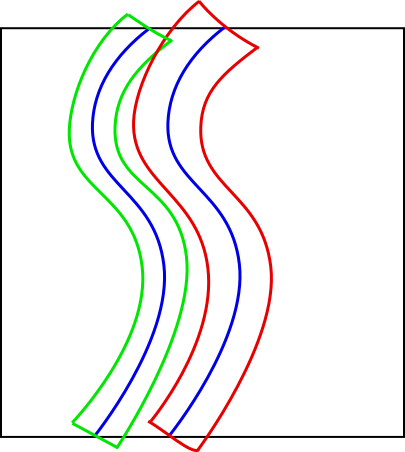
(a) Two tubular neighborhoods

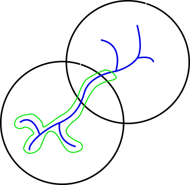
(b) From above: thin neighborhood

Proposition 5.8.

The dynamical vertical lamination in $\Delta^{2}_{R}$ can be extended to an open neighborhood.

Proof.

We consider $R^{\prime}>R$ and apply the previous lemma to the dynamical vertical lamination in $\Delta^{2}_{R^{\prime}}$. Let $2k^{2}\cdot\epsilon_{1}<(R^{\prime}-R)/2$, let $N$ be as in the previous lemma, and let $\epsilon_{2}>0$ be sufficiently small such that

$$2k^{2}\cdot\epsilon_{2}\cdot N<(R^{\prime}-R)/2,$$

where as before $k$ is an upper bound for the Lipschitz constant of the holonomy maps. We can cover the dynamical vertical lamination in $\Delta^{2}_{R}$ by tubular neighborhoods as in the previous lemma, and write $A_{1},\ldots,A_{N}$ for the partition into pairwise disjoint tubular neighborhoods. We may assume that $\epsilon_{1}$ and $\epsilon_{2}$ are chosen sufficiently small such that the $\lambda$-lemma can be applied to each tubular neighborhood of radius $k\cdot e_{i}$, for $i=1,2$.

We first apply the $\lambda$-lemma to each of the tubular neighborhoods $T_{i}(k^{2}\cdot\epsilon_{1},R^{\prime})$ in $A_{1}$, keeping only the leaves that intersect the tubular neighborhood of radius $k\cdot\epsilon_{1}$. Since the tubular neighborhoods of radius $k^{2}\cdot e_{1}$ are pairwise disjoint, it follows that the new leaves are all pairwise disjoint as well.

Note that while the dynamical leaves were global leaves, the new leaves are semi-local, and contained in the tubular neighborhoods in $A_{1}$. In order to guarantee that the new leaves are still graphs over the entire cores of the tubular neighborhoods in $A_{2},\ldots,A_{N}$ that they intersect, we reduce the radius of the bidisk $\Delta^{2}_{R^{\prime}}$ by $2k^{2}\cdot\epsilon_{1}$.

Note that the laminations constructed using the $\lambda$-lemma may not be Lipschitz. In order to guarantee preserve the modulus of continuity $k$ for each of the selected tubular neighborhoods that will be used in later steps, we keep only the newly constructed leaves that intersect a sufficiently thin neighborhood of the dynamical vertical lamination, see the two tubular neighborhoods illustrated in Figure 3(b), where the dynamical leaves are represented by the blue continuum, and only the new leaves in the small green neighborhood are kept. Since the holonomy maps will still be continuous, choosing a thin enough neighborhood of the dynamical vertical lamination will still guarantee that the leaves that intersect the tubular neighborhoods of radii $\epsilon_{2}$ and $k\cdot\epsilon_{2}$ will still be contained in the corresponding tubular neighborhoods of radii $k\cdot\epsilon_{2}$ and $k^{2}\cdot\epsilon_{2}$ respectively.

We continue with the tubular neighborhoods in $A_{2},A_{3},\ldots,A_{N-1}$, and finally to those in $A_{N}$, each time following the same procedure as above: first apply the $\lambda$-lemma to each tubular neighborhood of radius $k^{2}\cdot\epsilon_{2}$ in the current bidisk, keeping only those leaves that intersect the tubular neighborhood of radius $k\cdot\epsilon_{2}$, then decrease the radius of the bidisk by $k^{2}\cdot\epsilon_{2}$, and finally only keeping the newly constructed leaves in a very thin neighborhood of the dynamical vertical lamination in order to maintain the modulus of continuity.

By our choice of $\epsilon_{2}$ we end up with the required extended lamination on a bidisk of radius at least $R$. ∎

We will refer to this extension of the dynamical vertical lamination as the artificial vertical lamination, and denote it by $\mathcal{L}$. By slight abuse of terminology, we will also write $\mathcal{L}$ for the union of the vertical leaves, which gives a neighborhood of $J^{+}_{R}$. We may assume that the dynamical vertical lamination is extended to a thin enough neighborhood such that $\mathcal{L}$ is contained in the region where the dominated splitting is defined, and by continuity we may assume that its tangent bundle lies in the vertical cone field. From now on we write $\mathcal{N}(J^{+}_{R})$ for the region where both the cone field and the artificial vertical lamination are defined.

5.3. Adjusting the artificial vertical lamination on wandering domains

Note that there is no reason for the artificial vertical lamination $\mathcal{L}$ to be invariant under $f$. Here we discuss how to define and modify the lamination on the (hypothetical) wandering Fatou components.

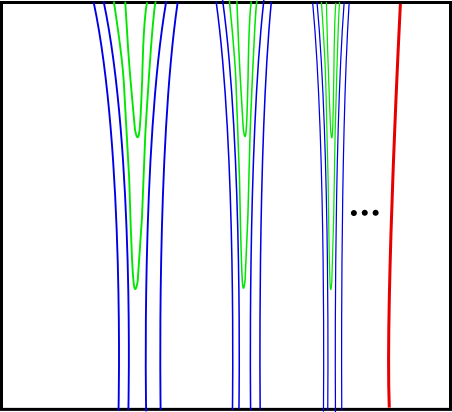
Figure 4. The pullback is not continuous in the limit

Recall the set ${\mathcal{V}}^{+}$ (2) foliated by stable manifolds $W^{s}(z)$. Let $U$ be a wandering Fatou component of $f$. As $f^{n}z\to J$ for any $z\in U$, we have: $U\subset{\mathcal{V}}^{+}$. So, $U$ is foliated by strong stable manifolds; we call it the dynamical foliation $\mathcal{F}_{U}$ of $U$. Putting these foliations together, we obtain the invariant dynamical foliation on the union $\mathcal{U}$ of all wandering components.

However, in general, this foliation cannot be extended to the closure of this union (see Figure 4). To deal with this problem, we combine this dynamical foliation on some “semi-local” wandering components with the non-dynamical extension on the others, to obtain a lamination of $\mathcal{U}\cap\Delta^{2}_{R}$ which is invariant everywhere except finitely many semi-local wandering components.

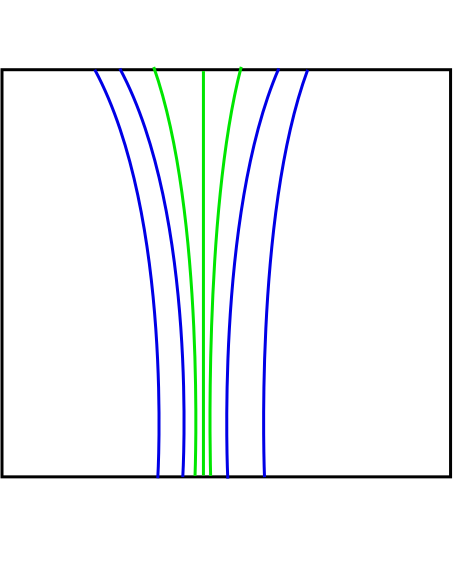
(a) Artificial vertical lamination

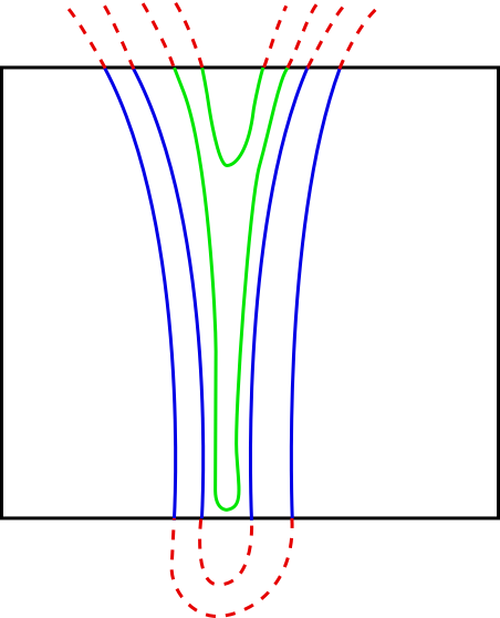
(b) Dynamical vertical lamination

Figure 5. Conflicting laminations in a wandering component

A semi-local wandering component $V$ is a connected component of $U\cap\Delta^{2}_{R}$. Note that there are at most finitely many semi-local wandering components $V\subset U\cap\Delta^{2}_{R}$ not contained in $\mathcal{N}(J^{+}_{R})$. We refer to such a component $V$ as a component with hole.

Let $V$ be a semi-local component with hole, let $V^{-1}$ be a connected component of $f^{-1}(V)\cap\Delta^{2}_{R}$, and assume that neither $V^{-1}$ nor any connected component of $f^{-n}(V^{-1})\cap\Delta^{2}_{R}$ has a hole. Then $V^{-1}$ is contained in $\mathcal{L}$ and hence foliated by vertical leaves. Note that vertical leaves in $\mathcal{L}$ sufficiently close to the (vertical) boundary of $V^{-1}$ are necessarily dynamical leaves, and recall that the dynamical vertical lamination is invariant under $f$. We modify the vertical lamination $\mathcal{L}$ by pulling back the leaves in $V^{-1}$ to all components of $f^{-n}(V^{-1})\cap\Delta^{2}_{R}$ for all $n\geq 2$.

If $V^{n}$ lies in $\mathcal{N}(J^{+}_{R})$ for all $n\geq n_{0}$, then the artificial vertical lamination on $V^{n_{0}}$ is dynamical, and we can pull back the dynamical lamination on $V^{n_{0}}$ to all components $V^{j}$ with $0\leq j\leq n_{0}$. See Figure 5 for a sketch of the two conflicting laminations that one obtains by pulling back the dynamical vertical lamination to $V^{-1}$. Note that the artificial vertical lamination near the boundary of the component is dynamical, and is therefore identical in both pictures.

By following this procedure for all grand orbits of Fatou components with holes, we obtain a lamination that is invariant on all but finitely many components, and for each bi-infinite orbit of components there is at most one step in which the lamination is not invariant. To be more precise, if ${V^{n}}_{n\in\mathbb{Z}}$ is a sequence of semi-local wandering components with $f(V^{n})\subset V^{n+1}$, then there is at most one $n\in\mathbb{Z}$ for which the leaves of the artificial vertical lamination in $V^{n}$ are not mapped into leaves of the lamination in $V^{n+1}$, and this can only occur when $V^{j}$ lies in the region of dominated splitting for $j\leq n$ but not for $j=n+1$.

5.4. Choice of horizontal line

In the one-dimensional argument we considered iterated inverse images of a given disk $D_{r}(z)$. This is problematic in the Hénon case. The reason is that such preimages are very likely to land at least partially outside of the bidisk $\Delta^{2}_{R}$. Instead, we will start with a flat horizontal complex line $\mathbb{L}_{0}$, map it forward by $f^{n}$, consider a small disk $V^{0}$ inside $f^{n}(\mathbb{L}_{0})\cap\Delta^{2}_{R}$, and consider the pullbacks $V^{1},\ldots V^{n}$ of this disk. Of course instead of working with a full horizontal line $\mathbb{L}_{0}$ it is equivalent to work with a disk of radius $R$.

We will now make a suitable choice for the horizontal line:

Lemma 5.9.

There exists $y_{0}\in\mathbb{C}$ with $|y_{0}|<R$ such that the artificial vertical lamination of $J^{+}$ is transverse to $\{y=y_{0}\}$.

Proof.

For each horizontal complex plane, the tangencies of this plane with the artificial vertical lamination are isolated, thus, by restricting the neighborhood of $J^{+}$ if necessary, there are at most finitely many tangencies. We can remove the tangencies one by one by making arbitrarily small perturbations for which the tangencies are transferred to nearby leaves in the Fatou set. More precisely, if a leaf is tangent to a horizontal plane, then each nearby vertical leaf is tangent to some nearby horizontal plane. Locally the number of tangencies, counted with multiplicities, is constant. Thus, we can take any nearby leaf in the Fatou set, take the horizontal plane for which that leaf is tangent, and reduce the number of tangencies in $J^{+}$ by at least one. After a finite number of perturbations we obtain a desired horizontal line $\{y=y_{0}\}$. ∎

Definition 5.10.

[choice of $\mathbb{L}_{0}$] From now on we fix $y_{0}$ so that the dynamical lamination of $J^{+}$ is transverse to $\mathbb{L}_{0}$, and so that $\mathbb{L}_{0}$ does not contain any parabolic periodic points.

It follows that the line $\mathbb{L}_{0}$ is transverse to the artificial vertical lamination in a sufficiently small neighborhood of $J^{+}$.

6. Uniformization of wandering components

In this section we will show that any wandering component $U$ can be uniformized by the straight cylinder $\mathbb{D}\times\mathbb{C}$ in such a way that the dynamical foliation of $U$ becomes vertical. It will imply a bound for the (appropriately understood) degrees of the maps $f^{n}|\,U$.

6.1. Contraction

Lemma 6.1.

For any wandering component $U$, the derivatives $\|df^{n}\|$ converge to $0$ uniformly on compact subsets of $U$.

Proof.

Replacing $U$ with its iterated image, if needed, we can ensure that all the images $U^{n}=f^{n}(U)$ lie in the domain of dominate splitting. Hence $U$ is filled with global strong stable manifolds $W^{s}(z)$.

Arguing by contradiction, we can find a sequence of unit vectors $v^{m}\in E^{c}(z^{m})$ converging to a vector $v\in E^{c}(z)$, $z\in U^{0}$, and a sequence of moments $n_{m}\to\infty$ such that

(4) $$\|df^{n_{m}}(v^{m})\|\geq{\varepsilon}>0.$$

Take a small horizontal disk $D\ni z$ tangent to $v$, and find a sequence of horizontal disks $D^{m}\ni z^{m}$ tangent to the $v^{m}$ and converging to $D$. Since the family of iterates is normal near $z$, the derivatives $d(f^{n}|\,D_{m})$ have a uniformly bounded distortion. Together with (4), this implies

$$\|df^{n_{m}}(w)\|\geq{\varepsilon}^{\prime}>0,\quad\forall\ w\in TD^{m},$$

so the images $f^{n_{m}}(D^{m})$ are horizontal disks of definite size. Hence the local stable manifolds through each of them fill a ball of definite radius. This contradicts the fact that these infinitely many balls must be disjoint yet bounded. ∎

Recall the set ${\mathcal{V}}^{+}$ (2) foliated by the strong stable manifolds $W^{s}(z)$. For $z\in{\mathcal{V}}^{+}$, let $\phi_{z}:\mathbb{C}\rightarrow W^{s}(z)$ be a uniformization of $W^{s}(z)$, normalized so that $\phi_{z}(0)=z$ and $\|d\phi_{z}(0)\|=1$. We note that $\phi_{z}$ is unique up to multiplication in $\mathbb{C}$ by a constant $e^{i\theta}$. Hence for $\zeta=\phi_{z}(u)\in W^{s}(z)$ we can define the (asymmetric) intrinsic distance as

$${\operatorname{dist}}^{i}(z,\zeta)=|u|,$$

which is independent of the choice of $\phi_{z}$.

Lemma 6.2.

(i) For $\zeta\in W^{s}_{\operatorname{loc}}(z)$, we have: ${\operatorname{dist}}^{i}(z,\zeta)\asymp\|z-\zeta\|;$

(ii) There exists an ${\varepsilon}>0$ with the following property: For any $\zeta\in W^{s}(z)\setminus W^{s}_{\operatorname{loc}}(z)$, there exists $n\asymp 1+\log^{+}({\varepsilon}^{-1}{\operatorname{dist}}^{i}(z,\zeta))$ such that $\|f^{n}z-f^{n}\zeta\|\geq{\varepsilon}.$

Proof.

(i) The linearizing maps $\phi_{z}$ are locally bi-Lipschitz with a constant continuously depending on $z$, which implies the first assertion.

(ii) Let us select ${\varepsilon}>0$ so that each $\phi_{z}$ maps the disk $\Delta_{\varepsilon}$ into $W^{s}_{\operatorname{loc}}(z)$. Since

(5) $$f^{n}\circ\phi_{z}(u)=\phi_{z_{n}}({\lambda}_{n}u)\quad{\mathrm{with}}\ {\lambda}_{n}=\|df^{n}_{z}|\,E^{s}\|,$$

the intrinsic distance is contracted at an exponential rate. Hence the number of iterates it takes for it to become of order $\epsilon$ depends logarithmically on $\mathrm{dist}^{i}(z,\zeta)$. Application of (i) concludes the proof. ∎

6.2. Global transversals

Recall from §5.3 that given a wandering component $U$, $\mathcal{F}_{U}$ stands for the dynamical vertical lamination of $U$ by the global stable manifolds $W^{s}(z)\approx\mathbb{C}$.

Let us say that $D$ is a global transversal to a wandering component $U$ if

(T1) $D$ is a non-singular holomorphic disk properly embedded into $U$;

(T2) $D$ is relatively compactly contained in a non-singular holomorphic curve $D^{\prime}$;

(T3) For any $z\in\bar{D}$, the curve $D^{\prime}$ is transverse to the stable line $E^{s}_{z}$ (see §4.0.3).

Lemma 6.3.

If $D$ is a global transversal to a wandering component $U$, then for $n$ large enough the images $f^{n}(D)$ are horizontal with respect to the cone field.

Proof.

By assumption (T3), the angle between the tangent line $T_{z}D$ and the stable line $E^{s}_{z}$ is bounded below by some $\alpha>0$ independent of $z\in D$. Hence it takes a bounded amount of iterates to bring $T_{z}D$ to a horizontal cone. ∎

Lemma 6.4.

Let $U$ be a wandering component, let $z\in U\cap\Delta^{2}_{R}$. Then $W^{s}(z)\subset U$ intersects a global transversal.

In particular, any wandering domain contains a global transversal.

Proof.

By Lemma 5.9, there exists a horizontal line $\mathbb{L}_{0}$ transverse to the dynamical vertical lamination on $J^{+}$. For large $n\in\mathbb{N}$ connected components of $f^{n}(U)\cap\Delta^{2}_{R}$ will be contained in an arbitrarily small neighborhood of $J^{+}$, and hence the dynamical vertical lamination in those components is transverse to $\mathbb{L}_{0}$. Since $f$ is substantially dissipative, the semi-local strong stable manifold $w^{s}_{R}(f^{n}(z))$ intersects $\mathbb{L}_{0}$ in a connected component $D_{n}\subset\mathbb{L}_{0}\cap f^{n}(U)$.

Since $f^{n}(U)$ is a Fatou component, the maximum principle implies that $D_{n}$ is simply connected. Let $D_{n}^{\prime}\subset\mathbb{L}_{0}$ be a slightly larger domain where the dynamical vertical lamination is still transverse to $\mathbb{L}_{0}$. Pulling back by $f^{n}$ gives the required $D\subset D^{\prime}$. ∎

Select a continuous unit vector field $v(z)\in E^{s}_{z}$ on $D^{\prime}$, and for $z\in D$, let $\phi_{z}:\mathbb{C}\rightarrow W^{s}(z)$ be the uniformization of $W^{s}(z)$ normalized so that $\phi_{z}(0)=z$ and $\phi^{\prime}_{z}(0)=v(z)$. Then we obtain a continuous map

(6) $$\Phi:D\times\mathbb{C}\rightarrow U,\quad(z,u)\mapsto\phi_{z}(u).$$

Our goal is to prove that $\Phi$ is a homeomorphism.

6.3. Holonomy group

Let $D$ and $\Delta$ be global transversals to $U$, let $z\in D_{1}$, and suppose that the global stable manifold $W^{s}(z)$ intersects $D_{2}$ in point $w\Delta$. Then holonomy induces a map $h$ from a neighborhood of $z$ in $D$ to a neighborhood of $w$ in $\Delta$.

Lemma 6.5.

The map $h$ admits a unique extension along any path $\gamma$ in $D_{1}$.

Proof.

Assume there exists a path $\gamma:[0,1]\rightarrow D$, $z^{0}=\gamma(0)$, such that $h$ extends along $\gamma:[0,1)\rightarrow D$ but does not extend to $z^{1}=\gamma(1)\in D$. We let

$$z^{t}=\gamma(t),\quad h(z^{t})=\Phi(z^{t},u^{t}),\quad t\in[0,1).$$

Since $h$ does not extend to $z^{1}$ it follows that

$${\operatorname{dist}}^{i}(z^{t},h(z^{t}))=|u^{t}|\to\infty\ {\mathrm{as}}\ t\to 1.$$

Otherwise we would have a subsequence $t_{k}\to 1$ with bounded $u^{t_{k}}$. Then we could take a limit point $u^{1}$ of the $u^{t_{k}}$ and obtain a local holonomy from $z^{1}$ to $h(z^{1})=\Phi(z^{1},u^{1})$. This local holonomy must then agree with the holonomy along $\gamma$ for $t$ close to $1$, giving a contradiction.

For $t\in[0,1)$, let ${\delta}^{t}$ be the “intrinsically straight” path in $W^{s}(z^{t})$ connecting $z^{t}$ with $h(z^{t})$:

$${\delta}^{t}:[0,u^{t}]\rightarrow W^{s}(z^{t}),\quad{\delta}^{t}(\cdot)=\Phi(z^{t},\cdot).$$

Let $D_{n}=f^{n}(D)$, $\gamma_{n}=f^{n}(\gamma)$, $z^{t}_{n}=f^{n}(z^{t})$, ${\delta}^{t}_{n}=f^{n}({\delta}^{t})$, and let $h_{n}=f^{n}\circ h\circ f^{-n}$ be the push-forward holonomy defined on $\gamma_{n}:[0,1)\rightarrow D_{n}$. By Lemma 6.1,

$$\operatorname{length}\gamma_{n}\to 0\ {\mathrm{and}}\ \operatorname{length}{\delta}^{0}_{n}\to 0\ {\mathrm{as}}\ n\to\infty,$$

where $\operatorname{length}$ stands for the Euclidean length. In particular, the path ${\delta}_{n}^{0}$ lies in $W^{s}(z^{0}_{n})$ for $n$ sufficiently big. On the other hand, there exists an ${\varepsilon}>0$ such that for any given $n$ and $t\in[1-\eta_{n},1)$ with $\eta_{n}\to 0$, $\operatorname{length}{\delta}^{t}_{n}\geq{\varepsilon}$. Let us select the smallest $t=t_{n}$ with this property.

Let us use a local coordinate system near $z_{n}^{0}$ with axes $E^{c}$ and $E^{s}$ at that point. Then the holonomy $h_{n}$ on the short path $\gamma_{n}(t))$, $0\leq t\leq t_{n}$, quickly goes from a small height (equal to $\operatorname{length}{\delta}_{n}^{0}$) to a definite height (of order ${\varepsilon}$), so it has a big average slope. It follows that somewhere either $\Delta_{n}$ or $D_{n}$ must have a small angle with the stable direction, contradicting the property that for large $n$ they are horizontal with respect to the cone field. ∎

Corollary 6.6.

Any local holonomy map $h$ extends to a homeomorphism $D\rightarrow\Delta$.

Proof.

Since $D$ is simply connected and any $h$ extends uniquely along all paths, the usual argument of the Monodromy Theorem implies that $h$ extends uniquely to a global continuous map $D\rightarrow\Delta$. Since the same is true for $h^{-1}$, it is a homeomorphism. ∎

In particular, we note that when $\Delta=D$, the holonomy maps form a group ${\mathcal{H}}_{D}$ of homeomorphisms of $D$.

Denote by $W^{s}(D)$ the union of the strong stable manifolds through $D$.

Lemma 6.7.

Let $D$ be a global transversal to a wandering component $U$. Then $U=W^{s}(D)$.

Proof.

It is immediate that $W^{s}(D)$ is an open subset of $U$. Let $z\in U\cap\overline{W^{s}(D)}$. Let $n\in\mathbb{N}$ such that $f^{n}(U)\cap\Delta^{2}_{R}$ is contained in ${\mathcal{V}}^{+}$. By Lemma 6.4 there exists a global transversal $\Delta\subset L$ intersecting $W^{s}_{R}(z_{n})$, or equivalently $z_{n}$ is contained in the semi-local strong stable manifold of some $w\in\Delta$. Then $W^{s}(\Delta)$ contains a neighborhood of $z_{n}$, and hence intersects $f^{n}(D)$. Thus, we obtain a local holonomy map from $\Delta$ to $f^{n}(D)$, which by Corollary 6.6 extends to a homeomorphism $h:\Delta\rightarrow D_{n}$. It follows that $W^{s}(D_{n})=W^{s}(\Delta)$, implying $z_{n}\in W^{s}(D_{n})$. We conclude that $z\in W^{s}(D)$, completing the proof. ∎

6.4. Uniformization

Proposition 6.8.

Let $D$ be a global transversal to a wandering component $U$. Then any stable manifold intersects $D$ in at most one point.

Proof.

Suppose for the purpose of a contradiction that a strong stable manifold intersects $D$ in two distinct points, and denote the induced holonomy homeomorphism by $h:D\rightarrow D$. Let us consider push-forward holonomies

$$h_{n}=f^{n}\circ h\circ f^{-n}:D_{n}\rightarrow D_{n},\quad{\mathrm{where}}\ D_{n}=f^{n}(D).$$

For any point $z\in D$ and $n$ big enough (depending on $z$), it is the holonomy along the local stable foliation in some flow box $B_{i}$ containing $z_{n}=f^{n}z$. By the $\lambda$-lemma [MSS83], $h_{n}$ is locally quasiconformal (“qc”) near $z_{n}$. Since a biholomorphic map $f^{n}$ does not change the dilation, $h$ is locally qc near $z$, with the same local dilatation (depending only on $B_{i}$ but not on $h$, $z$ and $n$). Since there are only finitely many flow boxes $B_{i}$ covering the whole domain of the dominated splitting, these local dilatations are uniformly bounded for all $h\in{\mathcal{H}}\equiv{\mathcal{H}}_{D}$ and $z\in D$. Hence each $h\in{\mathcal{H}}$ is globally qc on $D$ with uniformly bounded dilatation, so the holonomy group ${\mathcal{H}}$ acts uniformly qc on $D$.

Furthermore, ${\mathcal{H}}$ acts freely on $D$ since fixed points of the action would be tangencies between the stable foliation and $D$.

Moreover, for any point $z\in D$, the intersection $W^{s}(z)\cap D$ is discrete in the intrinsic topology of $W^{s}(z)$. Otherwise, there would exist distinct points $w^{m}=\phi_{z}(u^{m})\in D$ with bounded $u^{m}$. Then we could select a subsequence converging to a point $w=\phi_{z}(u)\in\overline{D}\subset D^{\prime}$, which would be a non-isolated point of the intersection $W^{s}(z)\cap D^{\prime}$.

In fact, this discreteness is uniform in the following sense: For any $M$ and any $z\in\overline{D}$, ${\operatorname{dist}}^{i}(z,hz)>M$ for all but finitely many holonomy homeomorphisms $h\in{\mathcal{H}}$. Indeed, if there is sequence $w^{m}=h_{m}(z^{m})=\Phi(z^{m},u^{m})$ with bounded $u^{m}$, then we can select a converging subsequence $u^{m}\to u$, $z^{m}\to z\in\overline{D}$, $w^{m}\to w\in\overline{D}$ so that $w=\Phi(z,u)=h(z)$ for some $h\in{\mathcal{H}}$. Then $h(z^{m})=\Phi(z^{m},t^{m})$ with $t^{m}\to u$, and hence $|t^{m}-u^{m}|\to 0$. But for $m$ big enough, both $\Phi(z^{m},t^{m})$ and $w^{m}=\Phi(z^{m},u^{m})$ lie in the same flow box $B$ around $w$. It follows that they lie in the same local leaf of $B$. Since the latter intersects $\overline{D}$ at a single point, we conclude that $w^{m}=h(z^{m})$, and hence $h_{m}=h$ (for all big enough $m$).

Let us now show that ${\mathcal{H}}$ acts properly discontinuously on $D$, i.e, for any two neighborhoods $Z$ and $W$ compactly contained in $D$, we have $h(Z)\cap W=\emptyset$ for all but finitely many $h\in{\mathcal{H}}$. Indeed, assume there is a sequence of distinct $h^{m}\in{\mathcal{H}}$ and of points $z^{m}\in Z$, $w^{m}=h^{m}(z^{m})\in W$. As we have just shown, ${\operatorname{dist}}^{i}(z^{m},w^{m})\to\infty$. Now we can apply our usual argument to arrive to a contradiction. Namely, there exist moments $n_{m}\to\infty$ that bring the points $z^{m}$ and $w^{m}$ to the same local stable manifold, implying that $\|f^{n_{m}}(z^{m})-f^{n_{m}}(w^{m})\|\asymp 1$, which contradicts to Lemma 6.1.

Hence the quotient $S=D/{\mathcal{H}}_{D}$ is a qc surface (i.e., a surface endowed with qc local charts with uniformly bounded dilatation). Taking any conformal structure (a Beltrami differential) $\mu$ on $S$ and pulling it back to $D$, we obtain an ${\mathcal{H}}$-invariant conformal structure on $D$. By the Measurable Riemann Mapping Theorem, there exists a qc map $\psi:D\rightarrow\mathbb{D}$ such that $g=\psi\circ h\circ\psi^{-1}$ is Möbius for any $h\in{\mathcal{H}}_{D}$.

Let $\zeta\in\mathbb{D}$ and denote its orbit by $\zeta_{n}=g^{n}(\zeta)$. Then the hyperbolic distance between $\zeta_{n}$ and $\zeta_{n+1}$ is independent of $n$ since it is preserved under holomorphic automorphisms. Let $z_{n}=\psi^{-1}(\zeta_{n})\in D$. Since $\psi$ is quasiconformal, it is a quasi-isometry, that is, $\psi$ expands the hyperbolic distance by a bounded factor for scales bounded away from zero. It follows that the hyperbolic distance between $z_{n}$ and $z_{n+1}$ is bounded for all $n$.

Since $g$ does not have fixed point in $\mathbb{D}$, the $\zeta_{n}$ converge to a Denjoy-Wolff point in $\partial\mathbb{D}$. Hence the sequence $(z_{n})_{n\in\mathbb{N}}$ escapes to the boundary $\partial D$. Since near the boundary the hyperbolic metric of $D$ explodes relatively the Euclidean metric of $D^{\prime}$, we conclude that

(7) $$\|z_{n}-z_{n+1}\|\to 0.$$

Note that all the points $z_{n}$ lie in the same stable manifolds $W^{s}(z)$, so we can measure the intrinsic distance between them. Property (7), together with Lemma 6.2, imply that ${\operatorname{dist}}^{i}(z_{n},z_{n+1})\to 0$. It follows that any limit point $q\in\overline{D}\subset D^{\prime}$ for $(z_{n})$ is a tangency between $D^{\prime}$ and $W^{s}(q)$, and this contradiction completes the proof. ∎

Remark 6.9.

The above application of the Measurable Riemann Mapping Theorem is a special case of Sullivan’s Theorem concerning uniformly qc group actions [Su81], [Tu86].

Since stable manifolds in $U^{0}$ intersect $D$ in a unique point, we conclude:

Corollary 6.10.

Let $D$ be a global transversal to a wandering component $U$. Then the uniformization $\Phi:D\times\mathbb{C}\rightarrow U$ is a vertically holomorphic homeomorphism.

6.5. Degree bound

Let $U^{0}$ be a semi-local wandering component of a wandering component $U$, and let $U^{n}$ be the component of $f^{n}(U)\cap\Delta^{2}_{R}$ containing $f^{n}(U^{0})$. we define the degree of $f^{n}:U^{0}\rightarrow U^{n}$ as the maximal number of semi-local dynamical leaves in $U^{0}$ that are mapped into a single semi-local dynamical leaf in $U^{n}$.

Lemma 6.11.

For any semi-local wandering component $U^{0}$, the degree of $f^{n}:U^{0}\rightarrow U^{n}$ is uniformly bounded over all $n$ (with a bound depending on $U^{0}$).

Proof.

By replacing $U^{0}$ with an appropriate $U^{m}$, we can ensure that all the domains $U^{n}$, $n\geq 0$, are contained in the neighborhood ${\mathcal{N}}(J^{+})$, so the dynamical and the artificial vertical laminations coincide on these domains. Note that degrees of compositions are sub-multiplicative, so a bound on the degrees of the maps $f^{n}:U^{m}\rightarrow U^{m+n}$ implies a bound on the degrees of the maps $f^{m+n}:U^{0}\rightarrow U^{m+n}$.

Let us consider a horizontal line $L=\mathbb{L}_{0}$, and let $t$ be the number of tangencies between $\mathbb{L}_{0}$ and the artificial vertical lamination. Let $L^{0}:=U^{0}\cap L$, and let $L^{n}:=f^{n}(L^{0})$.

As each semi-local dynamical leaf of $U^{0}$ intersects $L^{0}$, the degree of $f^{n}:U^{0}\rightarrow U^{n}$ is bounded by the maximal number of intersections between $L^{n}$ and the vertical leaves of $U^{n}$. Since the artificial vertical lamination of $U^{n}$ coincides with the (invariant) dynamical vertical lamination, the degree of $f^{n}:U^{0}\rightarrow U^{n}$ is bounded by the maximal number of intersections between $L^{n}$ and dynamical leaves of $f^{n}(U)$.

Let $D^{n}$ be a global transversal to $f^{n}(U)$ and let $\Phi_{n}:D^{n}\times\mathbb{C}\rightarrow f^{n}(U)$ be the corresponding uniformization. Then the maximal number of intersections between $L^{n}$ and dynamical leaves of $f^{n}(U)$ is equal to the degree $d$ of the horizontal projection $\Phi_{n}^{-1}(L^{n})\rightarrow D^{n}$. This projection is a branched covering since $L_{n}$ is properly embedded into $U^{n}$. By the Riemann-Hurwitz formula, $d$ equals at least one plus the number of tangencies (counted with multiplicities) between $L_{n}$ and the dynamical foliation. But the latter is preserved by the dynamics, so it equals the number of tangencies between $L^{0}$ and the dynamical foliation of $U^{0}$, which is bounded by $t$. The conclusion follows. ∎

7. Horizontal lamination and $\deg_{\mathrm{crit}}$

We let $U^{0}$ be a semi-local wandering Fatou component, and for $n\in\mathbb{N}$ we write $U^{-n}$ for a semi-local wandering components satisfying $f^{n}(U^{-n})\subset U^{0}$.

Assumption A. Let us say that a semi-local wandering component $U^{0}$ satisfies Assumption A if all possible choices of the domains $U^{-n}$, $n\geq 0$, are contained in $\mathcal{N}(J^{+}_{R})$ (defined at the end of §5.2), and thus in the domain of dominated splitting.

In what follows, through Corollary 7.5, we will assume that $U^{0}$ satisfies Assumption $A$.

We write $W^{-n}$ for a connected component of $U^{-n}\cap\mathbb{L}_{0}$, and consider holomorphic disks $f^{n}(W^{-n})\subset U^{0}$, ranging over all $n\in\mathbb{N}$ and all choices of $U^{-n}$ and $W^{-n}$. Since the horizontal line $\mathbb{L}_{0}$ is chosen so that it is transverse to the artificial vertical lamination near $J^{+}$, for $n$ sufficiently large the tangent spaces to the holomorphic disks $f^{n}(W^{-n})$ are contained in the horizontal cone field. In fact, by taking $n$ sufficiently large we may assume that the horizontal cone field is arbitrarily thin.

Let $z\in U^{0}$, and consider small bidisks $\Delta^{2}_{\rho}(z)\subset\Delta^{2}_{r}(z)\subset U^{0}$, with respect to affine coordinates contained in the horizontal respectively vertical cone field, and with boundary bounded away from $J^{+}$. For $\rho\ll r\ll 1$ any connected component of $f^{n}(W^{-n})\cap\Delta^{2}_{r}(z)$ intersecting $\Delta^{2}_{\rho}(z)$ is a horizontal graph. The collection of these graphs form a normal family, hence any sequence has a subsequence that converges locally uniformly. We consider the Riemann surfaces $\mathcal{S}_{\nu}$ that are locally given as uniform limits of these horizontal graphs.

Lemma 7.1.

If two limits $\mathcal{S}_{1}$ and $\mathcal{S}_{2}$ intersect, then they are equal.

Proof.

Assume for the purpose of a contradiction that $\mathcal{S}_{1}$ and $\mathcal{S}_{2}$ intersect in a point $z_{0}$, but that they locally do not coincide. Let us assume that $\mathcal{S}_{1}$ and $\mathcal{S}_{2}$ are locally given as limits of graph in respectively $f^{n_{j}}(W^{-n_{j}})$ and $f^{m_{l}}(W^{-m_{l}})$. In local coordinates $\Delta^{2}_{R}(z_{0})$ we can write $\mathcal{S}_{1}=\{y=\varphi(x)\}$ and $\mathcal{S}_{1}=\{y=\psi(x)\}$.

It follows that for large enough $j$ and $l$ the horizontal graphs in $f^{n_{j}}(W^{-n_{j}})$ and $f^{m_{l}}(W^{-m_{l}})$ intersect at a point near $z_{0}$.

Let $j$ and $l$ be large with, say, $n_{j}$ larger than $m_{l}$. Then it follows that there exists a point

$$\zeta_{m_{l}}\in f^{n_{j}-m_{l}}(W^{-n_{j}})\cap W^{-m_{l}}$$

for which $f^{m_{l}}(\zeta_{m_{l}})$ lies near $z_{0}$. As discussed above, for some large fixed $N$ independent of $l$ and $j$ the local graphs in $f^{N}\circ f^{n_{j}-m_{l}}(W^{-n_{j}})$ and $f^{N}(W^{-m_{l}})$ are both horizontal. Given that the map $f$ acts as an exponential contraction in the vertical direction, while being at most sub-exponentially contracting in the horizontal direction (by Lemma 4.2), it follows that near the point $f^{m_{l}}(\zeta_{m_{l}})$ the distance between the horizontal graphs in $f^{n_{j}}(W^{-n_{j}})$ and $f^{m_{l}}(W^{-m_{l}})$ shrinks exponentially fast as $l\rightarrow\infty$. Therefore, the limits $\varphi(\mathbb{D}_{r})$ and $\psi(\mathbb{D}_{r^{\prime}})$ coincide locally. Since they are both proper holomorphic disks, they must coincide globally, which gives a contradiction. ∎

We will refer to the collection of Riemann surfaces $\mathcal{S}_{\nu}$ as the horizontal lamination in $U^{0}$. It is clear that this lamination is contained in the backward Julia set $J^{-}$. Since $U^{0}$ is Kobayashi hyperbolic, each leaf is a hyperbolic Riemann surface. The leaves are locally given as limits of horizontal graphs, hence are themselves also horizontal.

Lemma 7.2.

The horizontal and the vertical laminations do not share leaves.

Proof.

Indeed, vertical leaves intersect the boundary of $\Delta^{2}_{R}$, while horizontal do not. ∎

Corollary 7.3.

For any semi-local component $U^{0}$ satisfying Assumption (A) the order of tangencies between horizontal and vertical leaves in $U^{0}$ is bounded.

Proof.

It follows from two observations:

$\bullet$ The order of tangencies between the leaves depends upper semi-continuous on the intersection point.

$\bullet$ Near $J^{+}$ the laminations are transverse. ∎

Corollary 7.4.

For any semi-local component $U^{0}$ satisfying Assumption (A), any preimage $U^{-j}$, and any component $W^{-j}$ of the horizontal slice ${\mathbb{L}}_{0}\cap U^{-j}$, the orders of tangency of the holomorphic disk $f^{j}(W^{-j})$ with the dynamical vertical foliation $\mathcal{F}_{U^{0}}$ is bounded.

Proof.

It is obvious for small $j$. For a large $j$, the disk $f^{j}(W^{-j})$ is a small perturbation of some horizontal leaf $L$ in $U^{0}$, so the order of its tangencies between $f^{j}(W^{-j})$ and $\mathcal{F}_{U^{0}}$ is bounded by the order of tangencies between $L$ and $\mathcal{F}_{U^{0}}$ . ∎

For a component $U^{0}$ satisfying Assumption (A), let us define $\deg_{\mathrm{crit}}(U^{0})$ as the maximum of the order of tangency between the above holomorphic disks $f^{j}(W^{-j})$ and the dynamical vertical foliation $\mathcal{F}_{U^{0}}$.

Corollary 7.5.

$\deg_{\mathrm{crit}}(U^{0})$ is bounded over all components $U^{0}$ satisfying Assumption A.

Proof.

In the case where all forward components $U^{n}$ are contained in $\mathcal{N}(J^{+})$ then the dynamical vertical lamination $\mathcal{F}_{U^{0}}$ is tangent to the vertical line field $E^{v}$, which is transverse to the horizontal lamination. Hence $\deg_{\mathrm{crit}}U^{0}=1$ in this case.

Therefore we only need to consider the case where some forward component $U^{n}$ is not contained in $\mathcal{N}(J^{+})$. Since $\deg_{\mathrm{crit}}(U^{0})$ is defined by means of two dynamical laminations, both invariant under $f$, it remains the same for all semi-local preimages $U^{-j}$ of $U^{0}$. Thus, it suffices to consider only those semi-local components $U^{n}$ for which $U^{n+1}$ does not satisfy Assumption A. Since there are only finitely many such components, the conclusion follows. ∎

Finally, let us get rid of Assumption A:

Lemma 7.6.

For an arbitrary semi-local component $U$, any component $W$ of the horizontal slice ${\mathbb{L}}_{0}\cap U$, and any integer $n\geq 0$, the orders of tangency of the holomorphic disk $f^{n}(W)$ with the dynamical vertical foliation $\mathcal{F}_{U^{n}}$ are bounded (where $U^{n}$ is the semi-local component containing $f^{n}(U)$).

Proof.

We already know this for components satisfying Assumption A, so let us deal with other components.

Assume $U^{n}\subset{\mathcal{N}}(J^{+})$, $n=0,1,\dots$. Then the vertical dynamical foliations on the $U^{n}$ are tangent to the vertical line field $E^{v}$. On the other hand, by the choice of ${\mathbb{L}}_{0}$, the slice $W$ is transverse to this line field. Thus, $W$ is transverse to $\mathcal{F}_{U}$. By invariance of the dynamical foliation, the forward iterates $f^{n}(W)$ are transverse to $\mathcal{F}_{U^{n}}$: no tangencies in play.

This leaves us with finitely many components $U$. For each of them, $W$ has finitely many tangencies with $\mathcal{F}_{U}$ counted with multiplicities (by construction of ${\mathbb{L}}$). By invariance of the dynamical foliations, $f^{n}(W)$ has the same number of tangencies with $\mathcal{F}_{U^{n}}$ for any integer $n\geq 0$. The conclusion follows. ∎

Definition 7.7.

[$\deg_{\mathrm{crit}}$] Let $\deg_{\mathrm{crit}}$ be the maximum of the orders of tangency that appear in the above lemma.

Corollary 7.8.

For any semi-local component $U^{0}$, any preimage $U^{-j}$, and any component $W^{-j}$ of the horizontal slice ${\mathbb{L}}_{0}\cap U^{-j}$, the order of tangency of the holomorphic disk $f^{j}(W^{-j})$ with the dynamical vertical foliation $\mathcal{F}_{U^{0}}$ is bounded by $\deg_{\mathrm{crit}}$.

8. Final preparations

The following is a rephrasing of Corollary 3.3.

Lemma 8.1.

Let $\epsilon>0$. Then there exists a domain $\Omega\subset\Delta^{2}_{R}$ for which

$$f^{-1}(\Omega)\cap\Delta^{2}_{R}\subset\Omega,$$

and

$$\left(J^{+}\cap\Delta^{2}_{R}\right)\bigcup\mathrm{(semi-local\ wandering\ components)}\setminus\{\;\mathrm{parabolic\;cycles}\;\}\subset\Omega,$$

and which satisfies two conditions:

1. For any $z\in J^{+}$ there exist $w\in\Delta^{2}_{R}$ with $|z-w|<\epsilon$ such that the semi-local leaf though $w$ does not intersect $\Omega$.

2. Any $z\in\Omega$ that does not lie in a wandering Fatou component lies $\epsilon$-close to $J^{+}$.

In several instances of the proof the value of the constant $\epsilon>0$ must be sufficiently small, which we will refer to by saying that $\Omega$ should be sufficiently thin. The domain $\Omega$ will only be fixed after all bounds on degrees and diameters are determined. To avoid a circular argument we should take care that the constants that appear in those bounds can be defined independently of the exact choice of $\Omega$. At this time we only guarantee that $\Omega$ is chosen sufficiently thin so that every point $z\in\Omega$ lies on a semi-local leaf of the artificial vertical lamination.

Lemma 8.2.

Given constants $d\in\mathbb{N}$, $r<1$ and $\mu>0$ there exists a constant $C=C(r,d,\mu)$ with the following property. For any hyperbolic Riemann surface $V$, and any proper quasiregular map $f:V\rightarrow\mathbb{D}$ of degree at most $d$ whose dilatation is bounded by $\mu$, the hyperbolic diameter of any connected component of $f^{-1}D_{r}(0)$ is bounded by $C$. For fixed $d,\mu$ the constant $C(r,d,\mu)$ converges to $0$ as $r\rightarrow 0$.

Proof.

The quasiregular map can be written as the composition of a proper quasiconformal homeomorphism with dilation bounded by $\mu$, with a proper holomorphic map of degree at most $d$. The statement holds for both of these maps, and hence also for the composition. ∎

Definition 8.3 (protected lifts).

Let $S\subset\Delta^{2}_{R}$ be a properly embedded holomorphic disk, bounded away from the horizontal boundary $\{|y|=R\}$. For a disk $D\subset\mathbb{L}_{0}$ consider all artificial vertical leaves through points in $D$. Write $V\subset S$ for a connected component of the set of intersection points of these artificial vertical leaves with $S$.

We say that $V$ is a lift of $D$ if the holonomy correspondence is proper, i.e. for any compact $E\subset D$ the intersection points of the leaves through $E$ with $V$ is compact.

We will consider lifts in $f^{j}\mathbb{L}_{0}\cap\Omega$. Let $t>1$ and consider two concentric disks $D_{r}(z)\subset D_{t\cdot r}(z)\subset\mathbb{L}_{0}$. If the disks $D_{r}(z)$ and $D_{t\cdot r}(z)$ can be lifted to $V_{r}(z)\subset V_{t\cdot r}(z)\subset f^{j}\mathbb{L}_{0}\cap\Omega$, then we say that $V_{r}(z)$ is a protected lift of $D_{r}(z)$. We define the degree of $V_{r}(z)$ as the maximal number of intersections with artificial vertical leaves.

Recall that the artificial vertical leaves intersect $\mathbb{L}_{0}$ transversally near $J^{+}$. Thus, for sufficiently small disks $D_{r}(z)\subset\mathbb{L}_{0}$ sufficiently close to $J^{+}$ the lift is traditional: a pullback under the holonomy map. However, if $D_{r}(z)$ intersects an artificial leaf non-transversally then the holonomy from $V_{r}(z)$ to $D_{r}(z)$ cannot be single valued, so we talk about the holonomy correspondence.

The properness of lifts is not automatic, and may be violated when an artificial vertical leaf through a disk $D$ is tangent to the boundary of $\Delta^{2}_{R}$. It is therefore possible that a disk $D_{r}(z)\subset\mathbb{L}_{0}$ that cannot be lifted, even when all artificial vertical leaves through $D$ are contained in $\Omega$. However, for every point $z\in\mathbb{L}_{0}$ for which the vertical leaf through $z$ intersects $f^{j}\mathbb{L}_{0}\cap\Omega$ there is a sufficiently small disk that can be lifted. Conversely every point in $f^{j}\mathbb{L}_{0}\cap\Omega$ is contained in some lift $V_{r}(z)$.

Lemma 8.4.

Let $V_{r}(z)\subset V_{t\cdot r}(z)$ be a protected lift of degree $d$. Then there exist a constant $C_{1}(\frac{1}{t},d)>0$ such that

$$\mathrm{diam}_{\Omega}V_{r}(z)\leq C_{1}(\frac{1}{t},d),$$

and given $d$ the constant $C_{1}(\frac{1}{t},d)$ converges to $0$ as $t\rightarrow\infty$.

Proof.

If $D_{t\cdot r}$ intersects artificial vertical leaves at most once, then the holonomy defines a proper quasi-regular map from $V_{t\cdot r}$ to $D_{t\cdot r}$. The degree of the holonomy map is then exactly the maximal number of intersections of $V_{t\cdot r}$ with leaves of the artificial lamination, which is $d$. It follows from Lemma 8.2 that the Poincaré diameter

$$\mathrm{diam}_{V_{t\cdot r}(z)}V_{r}(z)$$

is then bounded by $C(\frac{1}{t},d,\mu)$, for a bound $\mu$ on the order of qc-dilatation of the holonomy maps induced by the artificial vertical lamination. By definition of protected lifts we have $V_{t\cdot r}(z)\subset\Omega$, which implies the same bound on the Kobayashi diameter in $\Omega$.

Recall that the vertical lamination of $J^{+}$ is transverse to $\mathbb{L}_{0}$, hence the above discussion applies to sufficiently small disks in a sufficiently small neighborhood of $J^{+}$. By choosing $\Omega$ sufficiently thin, it follows that $D_{t\cdot r}(z)\subset\mathbb{L}_{0}$ intersects each vertical leaf in a unique point, unless $D_{t\cdot r}(z)$ intersects one of finitely many wandering Fatou components.

It is clear that for each given $D_{r}(z)\subset D_{t\cdot r}(z)\subset\mathbb{L}_{0}$ there does exist a bound on

$$\mathrm{diam}_{V_{t\cdot r}(z)}V_{r}(z),$$

depending only on the degree of $V_{t\cdot r}(z)$. Hence by compactness we obtain a bound when the radius $r$ is bounded away from zero. But when $r$ is sufficiently small, the disk $D_{t\cdot r}(z)$ either lies in a neighborhood of $J^{+}$ that guarantees that $D_{t\cdot r}(z)$ intersects each artificial vertical leaf at most once, or $D_{t\cdot r}(z)$ lies well inside one of a semi-local wandering Fatou component $U$, where $U$ is one of at most finitely many such components. It follows that

$$\mathrm{diam}_{U}V_{r}(z)\rightarrow 0$$

as $r\rightarrow 0$. Since $U\subset\Omega$, this completes the proof. ∎

Lemma 8.5.

There exists a constant $\epsilon>0$ such that the following holds. Let $V\subset\mathbb{L}_{0}$ be a holomorphic disk, and write $V^{j}=f^{j}(V)$. Suppose that for $j=0,\ldots,n$ we have $V^{j}\in\Delta^{2}_{R}$ and

$$\sup_{z\in V^{j}}d(z,J^{+})<\epsilon,$$

where $d(\cdot,\cdot)$ refers to the Euclidean distance in $\mathbb{C}^{2}$. Then each $V^{j}$ is transverse to the artificial lamination. If the Euclidean diameter of each $V^{j}$ is sufficiently small then it follows moreover that each $V^{j}$ has degree $1$.

Proof.

Recall that $\mathbb{L}_{0}$ is transverse to the artificial vertical lamination in a small neighborhood of $J^{+}$. Since the disks $V^{j}$ remain in the region of dominated splitting, their tangent spaces lie in some large horizontal cone field, while in a small neighborhood of $J^{+}$ the tangent spaces to the vertical leaves do not intersect those horizontal cones. Thus transversality follows, in fact with uniform bounds on the angles between the tangent spaces of the disks $V^{j}$ and the leaves of the artificial vertical lamination. It follows that sufficiently small disks will have degree $1$. ∎

Lemma 8.6.

Let $t>1$. There exists an $N_{0}=N_{0}(t)\in\mathbb{N}$ such that the following holds. For each protected lift $V_{r}(z)\subset V_{t\cdot r}(z)$ of disks $D_{r}(z)\subset D_{t\cdot r}(z)\in\mathbb{L}_{0}$, the preimage $V_{r}^{-1}(z)$ can be covered by protected lifts of at most $N_{0}$ disks $D_{r_{k}}(z_{k})\subset D_{2t\cdot r_{k}}(z_{k})$.

Moreover, in the particular case where the disk $D_{t\cdot r}(z)$ lies in a semi-local wandering component $U$, the lifts $V_{2t\cdot r_{k}}(z_{k})$ are all contained in the component $U^{-1}$. In all other cases, the lifts $V_{2t\cdot r_{k}}(z_{k})$ are all contained in $V_{tr}^{-1}(z)$.

Proof.

It is clear that for every $r>0$ and $z\in\mathbb{L}_{0}$ and every choice of protected lift $V_{r}(z)\subset V_{t\cdot r}(z)$, the disk $V_{r}^{-1}(z)$ can be covered with a finite number of protected lifts $V_{r_{k}}(z_{k})$ for which $V_{2tr_{k}}(z_{k})\subset V_{tr}^{-1}(z)$. Suppose for the purpose of a contradiction that there exists a sequence $(r,z,V_{r}(z))$ for which the minimal number of lifts needed converges to infinity.

By restricting to a subsequence we may assume that the lifts $V_{t\cdot r}(z)$ are either contained in wandering Fatou components, in periodic Fatou components, or all intersect $J^{+}$. We consider theses cases separately.

First suppose that the lifts $V_{t\cdot r}(z)$ are contained in wandering Fatou components. Suppose first that $V_{t\cdot r}(z)$ is contained a wandering domain $U$ where the artificial lamination is backwards invariant. By invariance the image of $V^{-1}_{t\cdot r}(z)$ in $\mathbb{L}_{0}$ under holonomy is independent of the choice of lift, and the argument is the same as in the one-dimensional setting: For disks of radius bounded away from zero the bound on $N_{0}$ follows from compactness. But sufficiently small disks are either contained in a small neighborhood of $J^{+}$, where the lamination is transverse to $\mathbb{L}_{0}$, or well inside wandering domains. In the latter case it is clear that $V^{-1}_{r}(z)$ can in fact be covered by a single lift. In the former case holonomy induces a quasiconformal map of bounded dilatation, which gives a bound on the distortion and thus on $N_{0}$.

Since the vertical lamination is invariant except in finitely many components, we may therefore assume that all $V_{t\cdot r}(z)$ are in one of the wandering components for which the vertical lamination is not backwards invariant. Recall that in this wandering Fatou component the vertical lamination is still invariant in a neighborhood of the boundary $J^{+}$. The bound on $N_{0}$ follows again when $r$ remains bounded away from zero, hence we may assume that $r\rightarrow 0$. But in that case the lifts are either very close to $J^{+}$, where the lamination is invariant and the bound on $N_{0}$ follows as above, or the lifts are bounded away from $J^{+}$. But then for sufficiently small $r$ the preimage $V_{r}^{-1}(z)$ can again be covered by a single lift $V_{\rho}(w)$ for which $V_{2t\cdot\rho}(w)\subset U^{-1}$.

Now suppose that the lifts $V_{t\cdot r}(z)$ are contained in periodic Fatou components. Recall that $\mathbb{L}_{0}$ was chosen to be transverse to the dynamical lamination near $J^{+}$. Thus, by making $\Omega$ sufficiently thin, we may assume that both $V_{t\cdot r}(z)$ and $V_{t\cdot r}^{-1}(z)$ are transverse to the vertical lamination, with angles bounded from below, see Lemma 8.5. Again it follows that holonomy from $\mathbb{L}_{0}$ to $V_{t\cdot r}^{-1}(z)$ and from $V_{t\cdot r}(z)$ back to $\mathbb{L}_{0}$ induces a quasiconformal map of bounded dilatation, which implies a bound on $N_{0}$.

The last case to be considered is when the lift $V_{t\cdot r}(z)$ intersects $J^{+}$. Suppose first that there exists a subsequence for which $r$ converges to zero. In that case $n$ must converge to infinity, since otherwise the preimages $V^{-i}_{t\cdot r}(z)$ are all contained in the domain of dominated splitting, which implies that the lifts $V_{t\cdot r}$ are horizontal, giving a bound on $N_{0}$. In fact, by Lemma 4.2 the contraction in the horizontal direction is sub-exponential, and hence in backwards time the expansion is sub-exponential, therefore we may assume that

$$n\geq\log_{\alpha}(r)$$

for any $\alpha>1$ and $r$ sufficiently small.

Since $n$ is large the disks $V_{t\cdot r}(z)$ must intersect $J^{+}$ in a point where $G^{-}$ is very close to zero, which implies that there is a nearby point $x\in J$ on the same local stable manifold. For each $x\in J$ there exists a small closed loop $\gamma$ around $x$ in $W^{s}(p)$ where $G^{-}$ is strictly positive. Consider a small disks through each point in $\gamma$, normal to $W^{s}(p)$, and therefore in particular horizontal, and denote the union of these horizontal disks by $\Gamma$. By making these horizontal disks sufficiently small, we can guarantee that $G^{-}$ is strictly positive on $\Gamma$. It follows that there exists an $N$ such that

$$f^{-N}(\Gamma)\cap\Delta^{2}_{R}=\emptyset.$$

By compactness of $J$ , we can find a uniform bound from above on the diameter of the $\gamma$, a uniform bound from below on the size of the horizontal disks through $\gamma$, and a uniform bound on $N$.

By the exponential contraction in the vertical direction and the fact that the inverse images $f^{-j}(V_{tr}(z))$ are all contained in the bidisk $\Delta^{2}_{R}$, it follows that $V_{tr}(z)$ is contained in a tubular neighborhood with radius of order $r^{\alpha}$ around the forward image of a horizontal disk $D$, (with radius of order $t\cdot r$) in a $f^{n-N}\Gamma(p)$, for some point $p\in J$, with similar estimates for $V^{-1}_{t\cdot r}(z)$ and $f^{-1}(D)$. Therefore it is sufficient to consider the respective lifts in $D$ and $f^{-1}(D)$, and the fact that these disks are horizontal implies a bound on $N_{0}$ by the same argument as above.

Thus the remaining lifts $V_{t\cdot r}(z)$ we need to consider have radius bounded away from zero and intersect $J^{+}$. By making $\Omega$ sufficiently thin we can therefore guarantee that for some $1<t_{2}<t$ the lift $V_{t_{2}\cdot r}(z)$ is contained in a wandering domain $U$. The existence of the bound $N_{0}$ follows by the same argument as when $V_{t\cdot r}(z)\subset U$.

∎

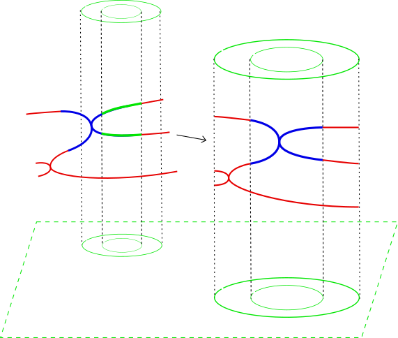
Figure 6. The set $V_{r}^{-1}$ is covered by lifts of disks $D_{r_{k}}(z_{k})\subset D_{t\cdot r_{k}}(z_{k})$.

Figure 6 illustrates the covering of $V_{r}^{-1}(z)$ by lifts of disks $D_{r_{k}}(z_{k})\subset D_{t\cdot r_{k}}(z_{k})$. The lift $V_{r}(z)$ and its inverse image $V_{r}^{-1}(z)$ are depicted in blue; the rest of the larger $V_{tr}(z)$ and $V_{t\cdot r}^{-1}(z)$ in red. In the sketch the vertical lamination is given by straight vertical lines. Two distinct lifts of a single disk $V_{r_{k}}(z_{k})$ are depicted in green.

Remark 8.7.

By construction the bound $N_{0}$ is independent of $\Omega$, that is, $N_{0}$ does not need to be changed when $\Omega$ is made smaller.

Let $U$ be a semi-local wandering domain on which the artificial lamination is not equal to the dynamical lamination. We will compare lifts of disks $D_{r}(z)\subset\mathbb{L}\cap U$ with respect to both laminations.

Proposition 8.8.

There exists $\delta=\delta(U)>0$ such that the following holds. Let $D\subset\mathbb{L}_{0}\cap U$ be a holomorphic disk of hyperbolic diameter (in $\mathbb{L}_{0}\cap U$) at most $\delta$, and let $V\subset f^{j}\mathbb{L}_{0}$ be a lift with respect to the dynamical lamination. Then $V$ is contained in a lift with respect to the artificial lamination of a protected disk $D_{\rho}(w)\subset D_{2\cdot\rho}(w)\subset\mathbb{L}_{0}\cap U$.

Proof.

Note that any connected component of $\mathbb{L}_{0}\cap U$ is simply connected. Therefore, as in the proof of Lemma 2.10, a subset $E\subset\mathbb{L}_{0}\cap U$ of sufficiently small hyperbolic diameter is contained in a disk $D_{r}(w)$ satisfying $D_{r}(w)\subset D_{2\cdot r}(w)\subset U$. Hence the proof is completed by showing that $V$ is a lift (with respect to the artificial lamination) of a set $E\subset\mathbb{L}_{0}\cap U$ of sufficiently small hyperbolic diameter.

Since the dynamical and artificial laminations coincide near the boundary of $U$, the statement holds trivially when $V$ is sufficiently close to the boundary. We will therefore consider lifts of disks $D$ that are bounded away from $\partial U$.

Recall from the previous section that the holomorphic disks $f^{n}(W^{-n})$ converge to the horizontal lamination. Both the horizontal leaves and the disks $f^{n}(W^{-n})$ cannot coincide with vertical dynamical leaves, hence for a sufficiently small tubular neighborhood $\mathcal{N}$ of a dynamical leaf, the intersection $f^{n}(W^{-n})\cap\mathcal{N}$ have arbitrarily small Euclidean diameters. Since we consider leaves that are bounded away from the boundary, small Euclidean diameters imply small Kobayashi diameters in $U$, and thus $V$ can be assumed to be a lift of some $E\subset\mathbb{L}_{0}\cap U$ of arbitrarily small hyperbolic diameter, which completes the proof.

∎

Definition 8.9.

[$\beta$] Let $\Lambda_{R}(a)$ be a vertical leaf that is either contained in $J^{+}$ or in a semi-local wandering domain, and assume that $\Lambda_{R}(a)$ is not one of the finitely many parabolic leaves in $J^{+}$ that were removed from $\Omega$. Then the leaf $\Lambda_{R}(a)$ is contained in $\Omega$. Note that the sets $f^{j}\mathbb{L}\cap\Delta^{2}_{R}$ stay bounded away from the horizontal boundary $\{|w|=R\}$. It follows that there exists an upper bound $\beta$, independent from $j\in\mathbb{N}$, on the Kobayashi diameter in $\Omega$ of the intersection of any vertical leaf $\Lambda_{R}(a)$ with any $f^{j}\mathbb{L}_{0}$. We note in particular that the constant $\beta$ can be chosen independently of $\Omega$.

Definition 8.10.

[$\mathrm{diam}_{\mathrm{max}}$] For $t>1$ and an integer $d\geq 2$ we define

$$\mathrm{diam}_{\mathrm{max}}(t,d):=2N_{0}(t)\cdot C_{1}(\frac{1}{2},d)+\beta.$$

In what follows $t$ will equal either $2$ or $2K$, where the constant $K$ will be introduced in Proposition 9.2. The integer $d$ will equal either $1$ or $\deg_{\mathrm{crit}}$.

Definition 8.11.

[big wandering domain] We say that a semi-local wandering domain $U$ is a big wandering domain if the vertical lamination on $U$ is not backwards invariant, or if there exist $j\in\mathbb{N}$ and $S\subset U\cap f^{j}\mathbb{L}_{0}$ of Kobayashi diameter

$$\mathrm{diam}_{U}S\leq\mathrm{diam}_{\max}(2,1)$$

intersecting a vertical leaf $\Lambda_{R}(a)$ for which $f^{-1}\Lambda_{R}(a)\cap\Delta^{2}_{R}$ has more than one component intersecting $f^{-1}S$.

We note that there are at most finitely many big wandering domains.

Definition 8.12.

[Regular wandering domains] A semi-local wandering domain $U$ is said to be regular if none of the components $U^{-n}$ for $n\geq 0$ are big wandering domains.

There exists only finitely many bi-infinite orbits of semi-local wandering domains that are not regular. A component that is not regular is called post-critical. Note that there at most finitely many grand orbits of semi-local wandering Fatou components that contain post-critical domains. If $U^{n}$ is regular but $U^{n+1}$ is post-critical then we say that $U^{n}$ is critical.

Definition 8.13.

[$\mathrm{deg}_{\mathrm{max}}$] Recall from Lemma 6.11 that the degree of the maps $f^{n}:U^{0}\rightarrow U^{n}$ is bounded from above by a constant independent of $n$. Thus, such a forward degree bound exists for each critical wandering component. Since there are only finitely many critical components, there exists a uniform bound, which we will denote by $\mathrm{deg}_{\mathrm{max}}$, analogously to the one-dimensional setting.

9. Diameter and degree bounds - proof for Hénon maps

Let us recall the constants and objects that play a role in the upcoming proofs, listed in the order of their dependency.

1. $\mathrm{deg}_{\mathrm{crit}}$ : The maximal local degree (Def 7.7).

2. $\mathbb{L}_{0}$ : Convenient choice of horizontal line (Def. 5.10).

3. $\beta$ : Upper bound on the Kobayashi diameter in artificial vertical leaves (Def. 8.9).

4. $N_{0}(t)$ : Maximal number of $t$-protected disks whose lifts cover $V_{r}^{-1}(z)$ (Lemma 8.6).

5. $C_{1}(\frac{1}{t},d)$ : Upper bound on the Kobayashi diameter for lifts in $\Omega$ (Lemma 8.4).

6. $\mathrm{deg}_{\mathrm{max}}$ : Bound on global degrees of iterates on critical wandering domains (Def. 8.13).

7. $K$: Defined in Prop. 9.2 below. We will consider protected lifts $V_{r}(z)\subset V_{2K\cdot r}(z)$.

8. $\mathrm{diam}_{\mathrm{max}}(t,d):=2N_{0}(t)\cdot C_{1}(\frac{1}{2},d)+\beta$ (Def. 8.10).

9. $\Omega$ : Domain of consideration, chosen sufficiently thin (Lemma 8.1).

In this section we prove the main estimates on the diameters and degree of lifts $V_{r}(z)$ and their preimages. Just as in the one-dimensional argument we distinguish between three different kinds of lifts. First we consider lifts that are deeply contained in wandering components, i.e. lifts of disks $D_{r}(z)$ for which $D_{K\cdot r}(z)$ is contained in the same component for a sufficiently large constant $K$. Afterwards we consider the two remaining cases, namely lifts of disks that are not contained in wandering components, and lifts of disks $D_{r}(z)$ that are contained in wandering components but for which the protecting disks $D_{K\cdot r}(z)$ are not.

9.1. Lifts deeply contained in wandering domains.

In what follows we let $(U^{n})_{n\in\mathbb{Z}}$ be a bi-infinite orbit of semi-local wandering Fatou components, and consider protected lifts $V_{r}\subset V_{t\cdot r}$ for which $V_{t\cdot r}$ is contained in one of the domains $U^{n}$. As post-critical components are harder to deal with than regular components, we start with the latter.

Lemma 9.1.

Let $U^{n}$ be a regular wandering semi-local Fatou component and let $V_{r}(z)\subset V_{2r}(z)\subset f^{j}\mathbb{L}_{0}\cap U^{n}$ be protected lifts of disks $D_{r}(z)\subset D_{2r}(z)\subset\mathbb{L}_{0}$. Then for $i=0,\ldots,j$ we have

$$\mathrm{diam}_{\Omega}V_{r}^{-i}(z)\leq\mathrm{diam}_{\max}(2,1)$$

and

$$\mathrm{deg}V_{r}^{-i}(z)=1.$$

Proof.

We will assume the statement holds for a given $j\in\mathbb{N}$, and proceed to prove it for $j+1$. By Lemma 8.6 the holomorphic disk $V^{-1}_{r}(z)$ can be covered by lifts $V_{r_{k}}(z_{k})$ of at most $N_{0}$ disks $D_{r_{k}}(z_{k})\subset D_{4\cdot r_{k}}(z_{k})\subset\mathbb{L}_{0}\cap U^{n-1}$. By the induction assumption each $V_{2\cdot r_{k}}^{-i}(z_{k})$ has degree $1$, and thus we obtain the estimates

$$\mathrm{diam}_{U^{n-i-1}}V_{r_{k}}^{-i}(z_{k})\leq C_{1}(\frac{1}{2},1).$$

Note that a priori we do not have a bound on the number of lifts $V_{r_{k}}(z_{k})$. Since $U^{n}$ is regular, the vertical lamination on the components $(U^{n-i})_{i\geq 0}$ is invariant. Let $x\in V_{r}(z)$, and write $x_{-i}=f^{-i}(x)$. Each point in a lift $V_{r_{k}}(z_{k})$ can be connected to the semi-local leaf $\Lambda(x_{-1})$ by a path that travels through at most $N_{0}$ other lifts $V_{r_{l}}(z_{l})$. Hence it follows that

$$\mathrm{diam}_{U^{n-1}}V_{r}^{-1}(z)\leq\mathrm{diam}_{\max}(2,1).$$

Recall that by Definitions 8.11 and 8.12 of respectively big and regular Fatou components, this bound on the hyperbolic diameter in $U^{n-1}$ of $V_{r}^{-1}(z)$ implies that $\Lambda(x_{-2})$ is the unique semi-local leaf in $f^{-1}\Lambda(x_{-1})\cap\Delta^{2}_{R}$ that intersects $V_{r}^{-2}(z)$. The same argument as above gives the same bound on the hyperbolic diameter in $U^{n-2}$ of $V_{r}^{-2}(z)$. Continuing by induction on $i$ gives

$$\mathrm{diam}_{U^{n-i}}V_{r}^{-i}(z)\leq\mathrm{diam}_{\max}(2,1),$$

for all $i\leq j$. We obtain the required bounds on the hyperbolic diameters in $\Omega$, as $\Omega$ contains all semi-local wandering components. Since the semi-wandering component $U$ is regular it follows that

$$\mathrm{deg}V_{r}^{-i}(z)=1$$

for $i=0,\ldots,j$. ∎

Proposition 9.2.

There exists a constant $K>0$ such that the following holds. Let $U^{n}$ be a semi-local wandering component, and let $V_{r}(z)\subset V_{K\cdot r}(z)\subset f^{j}\mathbb{L}_{0}\cap U^{n}$ be protected lifts of disks $D_{r}(z)\subset D_{K\cdot r}(z)\subset\mathbb{L}_{0}$. Then for all $i\leq j$ we have

$$\mathrm{diam}_{\Omega}V_{r}^{-i}(z)\leq\mathrm{diam}_{\max}(2,1),$$

and

$$\mathrm{deg}V_{r}^{-i}(z)\leq\mathrm{deg}_{\mathrm{crit}}.$$

Proof.

Write $U^{n-i}$ for the semi-local wandering Fatou component in $f^{-i}U^{n}\cap\Delta^{2}_{R}$ that contains the lift $V_{r}^{-i}(z)$. By renumbering the orbit $U^{j}$ we may assume that $U^{0}$ is critical. It follows from the previous lemma that $K\geq 2$ suffices when $n\leq 0$, so let us suppose that $n>0$.

We first consider the hyperbolic diameters in components $U^{n-i}$, for $i\leq n$. We write $D_{r}(z)\subset D_{k\cdot r}(z)\subset U^{n}\cap\mathbb{L}_{0}$ for the disks giving the lifts $V_{r}(z)\subset V_{K\cdot r}(z)$. We also consider the lifts these disks to $f^{i}\mathbb{L}_{0}$.

Recall from the proof of Lemma 6.4 that for $n$ sufficiently large any connected component $D$ of $\mathbb{L}_{0}\cap U^{n}$ is a global transversal. The composition of $f^{i}$ with holonomy from $f^{i}(\mathbb{L}_{0}\cap U^{n-i})\rightarrow D$, induces quasi-regular maps, whose degrees are bounded by $\mathrm{deg}_{\mathrm{m}ax}$ and have bounded dilatation. It follows that by making $K$ sufficiently large, the hyperbolic diameter of the preimage in $\mathbb{L}_{0}\cap U^{n-i}$ can be made arbitrarily small. Note that $V^{-i}_{r}(z)$ is a lift of this pre-image with respect to the dynamical lamination. It follows that the Kobayashi diameter of $V^{-i}_{r}(z)$ in $U^{-i}$, and thus also in $\Omega$, can therefore be made arbitrarily small by choosing $K$ large.

Let us consider the finitely many values of $n$ for which we do not know that $D$ is a global transversal. For any fixed $n$, making $K$ sufficiently large implies that $V_{r}^{-i}(z)$ is contained in an arbitrarily small neighborhood of a dynamical leaf, and thus we immediately obtain the same bounds on the hyperbolic diameter in $\mathbb{L}_{0}\cap U^{n-i}$. Therefore we can drop the assumption that $n$ is sufficiently large.

We now consider the artificial vertical lamination on $U^{0}$. We have seen that $V_{r}^{-i}(z)$ is the lift with respect to the dynamical lamination of a set $E\subset\mathbb{L}_{0}\cap U^{0}$, whose hyperbolic diameter can be made arbitrarily small by choosing $K$ sufficiently large. Lemma 8.8 implies that $V_{r}^{-i}(z)$ is contained in the lift of a disk $D_{\rho}(w)\subset D_{2\cdot\rho}(w)\subset\mathbb{L}_{0}\cap U^{0}$ with respect to the artificial lamination when the hyperbolic diameter of $E$ is less than $\delta=\delta(U^{0})$. Since there are only finitely many critical components $U^{0}$, the constant $\delta$ can be chosen independently of the critical component, and thus $K$ can be chosen independently as well.

By applying Lemma 9.1 to the lift of the disk $D_{\rho}(w)$ we obtain the required diameter bounds on $V^{-i}_{r}(z)$ for $n\leq i\leq j$, as well as

$$\mathrm{deg}V^{-i}_{r}(z)=1$$

for $n\leq i\leq n$. Hence if $K$ is chosen sufficiently large it follows that

$$\mathrm{deg}V^{-i}_{r}(z)\leq\mathrm{deg}_{\mathrm{crit}}$$

for all $i\leq j$. ∎

9.2. Lifts that are not deeply contained.

We are ready to prove the main technical result:

Proposition 9.3.

Let $z\in\Omega$ and let $r>0$ be such that $D_{2K\cdot r}(z)\subset\Omega$. Then for every $j\in\mathbb{N}$ and any lift $V_{r}(z)\subset f^{n}\mathbb{L}_{0}$ one has:

$$\mathrm{diam}_{\Omega}V_{r}^{-j}(z)\leq\mathrm{diam}_{\mathrm{max}}(2K,\deg_{\mathrm{crit}}),$$

and

$$\mathrm{deg}V_{r}(z)\leq\mathrm{deg}_{\mathrm{crit}}.$$

Proof.

Having previously dealt with lifts that are sufficiently deeply contained in wandering domains, we only need to consider the two other cases: lifts are either not contained in a wandering component, or those that are contained in a wandering component, but lifts of disks $D_{r}(z)$ for which $D_{K\cdot r}(z)$ intersects $J^{+}$.

We again assume the induction hypothesis that both bounds hold for all $i\leq j$, and proceed to prove the statements for $j+1$. We will first prove the induction step under the assumption that $D_{r}(z)$ is not contained in a wandering domain, and afterwards deal with the case where $D_{r}(z)$ is contained in a wandering domain. The result in the former case will be used to prove the latter.

Case 0. Let us first consider the situation where $V_{r}(z)$ is contained in a periodic Fatou component. By choosing $\Omega$ sufficiently thin we can guarantee that $V_{r}(z)$ is horizontal and that the disks $D_{r}(z)$ and $D_{2k\cdot r}(z)$ are arbitrarily small. It follows that $V_{r}(z)$ must have degree $1$. Hence we can cover $V_{r}^{-1}(z)$ with at most $N_{0}(2K)$ protected lifts $V_{r_{k}}(z_{k})\subset V_{4K\cdot r_{k}}(z_{k})\subset V_{2K\cdot r}(z)$. It follows by the induction assumption that the disks $V_{2\cdot r_{k}}(z_{k})$ all have degree at most $\mathrm{deg}_{\mathrm{crit}}$. Recall from the proof of Lemma 8.4 that the Poincaré diameter of $V_{r_{k}}(z_{k})_{\nu}$ with respect to $V_{2\cdot r_{k}}(z_{k})_{\nu}$ is bounded by $C_{1}(\frac{1}{2},\mathrm{deg}_{\mathrm{crit}})$. Since $f$ is an automorphism, we obtain the same bounds for the pairs $V^{-i}_{r_{k}}(z_{k})_{\nu}\subset V^{-i}_{2\cdot r_{k}}(z_{k})_{\nu}$, and since each $V^{-i}_{2\cdot r_{k}}(z_{k})_{\nu}\subset\Omega$, therefore we have the bounds

$$\mathrm{diam}_{\Omega}V^{-i}_{r_{k}}(z_{k})\leq C_{1}(\frac{1}{2},\mathrm{deg}_{\mathrm{crit}}).$$

This implies that

$$\mathrm{diam}_{\Omega}V_{r}^{-i}(z)\leq N_{0}(2K)\cdot C_{1}(\frac{1}{2},\mathrm{deg}_{\mathrm{crit}}),$$

which in turn gives the necessary degree bounds.

Case 1. Now assume that $V_{r}(z)$ is not contained in a Fatou component. Then there exists $y_{0}\in D_{r}(z)\cap J^{+}$, and we let $x_{0}\in V_{r}(z)$ lie in the semi-local vertical leaf through $y_{0}$, which we denote by $\Lambda_{R}(x_{0})$. We similarly write $\Lambda_{R}^{-i}(x_{0})$ for the semi-local leaf through $f^{-i}(x_{0})$, which by invariance of the vertical lamination on $J^{+}$ equals the connected component of $f^{-i}(\Lambda_{R}(x_{0}))$ that contains $f^{-i}(x_{0})$.

Cover $V^{-1}_{r}(z)$ by protected lifts $V_{r_{k}}(z_{k})_{\nu}\subset V_{4K\cdot r_{k}}(z_{k})_{\nu}\subset\Omega$ of at most $N_{0}(2K)$ disks $D_{r_{k}}(z_{k})\subset D_{4K\cdot r_{k}}(z_{k})\subset\mathbb{L}_{0}$. The induction hypothesis implies that the degree of each lift $V_{2\cdot r_{k}}(z_{k})_{\nu}$ is bounded by $\mathrm{deg}_{\mathrm{crit}}$, hence as above we obtain

$$\mathrm{diam}_{\Omega}V^{-i}_{r_{k}}(z_{k})_{\nu}\leq C_{1}(\frac{1}{2},\mathrm{deg}_{\mathrm{crit}}).$$

As before we do not have an a priori estimate on the number of lifts $V_{r_{k}}(z_{k})_{\nu}$. We apply the same induction argument as in Proposition 9.2. By choosing $\Omega$ sufficiently thin we can guarantee that the Euclidean diameter of $V_{r}(z)$ is sufficiently small, so that for each vertical leaf $\Lambda_{R}(a)$ intersecting $V_{r}(z)$ there is a unique component of $f^{-1}\Lambda_{R}(a)\cap\Delta^{2}_{R}$ intersecting $V_{r}^{-1}(z)$.

Any point in $V^{-1}_{r}(z)$ can then be connected to a point in $\Lambda_{R}^{-1}(x_{0})$ by a path that passes through at most $N_{0}(2K)$ lifts $V_{r_{k}}(z_{k})_{\nu}$. By the definition of $\beta$ it follows that

$$\mathrm{diam}_{\Omega}V_{r}^{-1}(z)\leq\mathrm{diam}_{\mathrm{max}}(2K,\deg_{\mathrm{crit}}).$$

Hence we can continue the induction procedure, and obtain

$$\mathrm{diam}_{\Omega}V_{r}^{-i}(z)\leq\mathrm{diam}_{\mathrm{max}}(2K,\deg_{\mathrm{crit}})$$

for all $i\leq j$.

By choosing $\Omega$ sufficiently thin it follows from Lemma 8.5 that each $V^{-i}_{r}(z)$ is transverse to the artificial vertical lamination and that

$$\mathrm{deg}V^{-i}_{r}(z)=1$$

for all $i\leq j$, completing the proof for disks $D_{r}(z)$ that are not contained in a wandering component.

Case 2. In the remainder of this proof we assume that $D_{r}(z)$ is contained in a semi-local wandering component $U$, but that $D_{K\cdot r}(z)$ is not contained in $U$. We again cover $V^{-1}_{r}(z)$ with protected lifts $V_{r_{k}}(z_{k})_{\nu}\subset V_{4K\cdot r}(z_{k})_{\nu}\subset f^{j-1}\mathbb{L}_{0}\cap\Omega$ of at most $N_{0}(2K)$ disks $D_{r_{k}}(z_{k})\subset D_{4K\cdot r}(z_{K})\subset\mathbb{L}_{0}$, and by induction obtain the diameter bounds

$$\mathrm{diam}_{\Omega}V_{r_{k}}^{-i}(z_{k})_{\nu}\leq\mathrm{diam}_{\mathrm{max}}(2K,\deg_{\mathrm{crit}}).$$

Again the difficulty lies in the fact that a priori we do not have a bound on the number of lifts $V_{r_{k}}(z_{k})_{\nu}$. As before we will obtain the diameter bounds for each inverse image $V_{r}^{-i}(z)$ by connecting the disks $V_{r_{k}}^{-i+1}(z_{k})_{\nu}$ to a single semi-local vertical leaf.

Write $W$ for the component of $U\cap\mathbb{L}_{0}$ that contains $D_{r}(z)$, and let $w\subset\partial W$ be such that $|z-w|$ is minimal, and write $[z,w]\subset\mathbb{L}_{0}$ for the closed interval.

Consider the disk $D_{\frac{r}{2}}(w)$. Since $D_{K\cdot r}(w)\subset D_{2K\cdot r}(z)$ it follows that $D_{K\cdot r}(w)\subset\Omega$. Hence the disk $D_{\frac{r}{2}}(w)$ satisfies the conditions of the previously discussed case, and we obtain the estimates

$$\mathrm{diam}_{\Omega}V^{-i}_{\frac{r}{2}}(w)\leq\mathrm{diam}_{\mathrm{max}}(2K,\deg_{\mathrm{crit}})$$

for any protected lifts $V_{\frac{r}{2}}(w)\subset V_{K\cdot r}(w)\subset f^{j}\mathbb{L}_{0}\cap\Omega$ of the disks $D_{\frac{r}{2}}(w)\subset D_{K\cdot r}(w)$.

The interval $[z,w]$ can be covered by the disk $D_{\frac{r}{2}}(w)$, plus a bounded number of disks

$$D_{s_{1}}(w_{1}),\ldots,D_{s_{N_{1}}}(w_{N_{1}}),$$

each satisfying $D_{K\cdot s_{\nu}}(w_{\nu})\subset U^{n}$. The maximal number of disks needed is bounded by a constant $N_{1}\in\mathbb{N}$ that only depends on $K$, see Figure 1.

Write

$$V_{s_{\nu}}(w_{\nu})_{\xi}\subset V_{K\cdot s_{\nu}}(w_{\nu})_{\xi}\subset f^{j}\mathbb{L}_{0}\cap\Omega$$

for protected lifts of the disks $D_{s_{\nu}}(w_{\nu})\subset D_{K\cdot s_{\nu}}(w_{\nu})$. It follows that these lifts satisfy the conditions of Proposition 9.2, and hence their preimages satisfy

$$\mathrm{diam}_{\Omega}V^{-i}_{s_{\nu}}(w_{\nu})_{\xi}\leq\mathrm{diam}_{\mathrm{max}}(2K,\deg_{\mathrm{crit}}).$$

As in case 1 we obtain a bound on the hyperbolic distance of each point $f^{-i}(z)$ to $\partial U^{-i}\subset J^{+}$. By choosing $\Omega$ sufficiently thin, it follows that the points $f^{-i}(z)$ can all be assumed to lie arbitrarily close to $J^{+}$. In particular we may assume that the vertical leaf through each $f^{-i}(z)$ is dynamical, and these semi-local leaves $\Lambda_{R}^{-i}(z)$ are in particular invariant under $f$. Recall from Definition 8.9 that

$$\mathrm{diam}_{\Omega}f^{j-i}\mathbb{L}_{0}\cap\Lambda_{R}^{-i}(z)$$

is bounded by $\beta$. Hence we can use the same argument as in case (1), using $\Lambda_{R}^{-i}(z)$ instead of a semi-local leaf in $J^{+}$, to obtain the required diameter and degree bounds. ∎

10. Consequences

As before we will assume that the Hénon map $f$ is substantially dissipative and admits a dominated splitting on $J$.

Lemma 10.1.

There are no wandering Fatou components.

Proof.

Suppose for the purpose of a contradiction that there does exist a wandering Fatou component $U$. Without loss of generality we may assume that $U$ intersects $\Delta^{2}_{R}$. Since $U\cap\Delta^{2}_{R}$ is foliated by semi-local strong stable manifolds, the intersection $U\cap\mathbb{L}_{0}$ is a non-empty relatively open set. Let $D$ be a holomorphic disk relatively compactly contained in $U\cap\mathbb{L}_{0}$. By construction, we may assume that $\Omega$ is sufficiently thin and $D\subset U\cap\mathbb{L}_{0}$ is sufficiently large such that the hyperbolic diameter of $D$ in $\Omega^{\prime}$ is larger than $\mathrm{diam}_{\mathrm{max}}$.

Since $U$ lies in the Fatou set there exists a sequence $(n_{j})$ for which $f^{n_{j}}$ converges uniformly on compact subsets of $U$ to a map $h:U\rightarrow J$. By the dominated splitting the image $h(U)$ is a point $p\in J$, and without loss of generality we may assume that $p$ is not contained in a parabolic cycle. Let $D_{r}(p)\subset D_{2r}(p)\subset\Omega$ be a transverse disk. Since $D$ is relatively compact in $U$, it follows that for sufficiently large $j$ the image $f^{n_{j}}(D)$ is contained in a lift of $D_{r}(p)$ in $f^{n_{j}}(\mathbb{L}_{0}$. But then it follows from Proposition 9.3 that the hyperbolic diameter of $D$ in $\Omega^{\prime}$ is bounded by $\mathrm{diam}_{\mathrm{max}}$, leading to a contradiction. ∎

Lacking wandering domains the proof of Proposition 9.3 becomes considerably simpler. An immediate consequence is a better degree bound.

Corollary 10.2.

The constant $\mathrm{deg}_{\mathrm{crit}}$ can be taken equal to $1$.

Proof.

Since there are no wandering Fatou components, it follows from the proof of Proposition 9.3 that the degree of the disk $V_{r}$ is bounded by the degree of the disk $V_{n}$, which is a small straight disk contained in $\mathbb{L}_{0}$. Recall that $y_{0}$ was chosen so that there are no tangent intersections between $\mathbb{L}_{0}$ and the dynamical vertical lamination on $J^{+}$. Now that we know that there are no wandering Fatou components, the set $\Omega$ can be constructed as an arbitrarily thin neighborhood of $J^{+}_{R}$. Hence we may assume that there are no tangencies in $\mathbb{L}_{0}$ with the artificial vertical lamination in $\Omega$. Since the disks $V_{n}$ may be assumed to have arbitrarily small Euclidean diameter, it follows that $V_{n}$ intersects each vertical leaf in at most one point. ∎

Proposition 10.3.

Let $x\in\Omega\cap J$. Then there exists a local unstable manifold through $x$.

Proof.

For each $n\in\mathbb{N}$, the semi-local strong stable manifold $W^{s}_{R}(f^{-n}(x))$ must intersect the horizontal disk $\mathbb{L}_{0}$. Let $y_{n}$ be such an intersection point. Since the degree of the semi-local strong stable manifolds is uniformly bounded and $f$ is uniformly contracting on the family of strong stable manifolds, it follows that $f^{n}(y_{n})$ converges exponentially fast to $x$. Moreover, by the exponential contraction in the vertical direction, it follows that locally the disks $D_{n}\subset f^{n}\mathbb{L}_{0}$ passing through $f^{n}(y_{n})$ converge to a holomorphic disk through $x$, which we denote by $D$.

We claim that $D$ must be an unstable manifold, i.e. that the diameter of $f^{-n}(D)$ converges to $0$. By the exponential contraction in the vertical direction it suffices to show that the diameter of $f^{-n}(D_{n})$ converges to zero. Suppose that this is not the case. Recall that the diameters of the disks $f^{-n}(D_{n})$ are uniformly bounded, hence are given by images of a normal family of holomorphic maps. Hence if the diameters do not converge to zero, then there is a subsequence $(n_{j})$ for which $f^{-n_{j}}(D_{n_{j}})\subset\mathbb{L}_{0}$ converges to a holomorphic disk $E$, necessarily intersecting $J^{+}$. By construction $\mathbb{L}_{0}$ is transverse to $J^{+}$, hence it follows that $E$ must intersect vertical leaves through points in the basin of infinity, say in a point $t$. Since those vertical leaves must be contained in the basin of infinity, so must $t$. Note that since $t\in E$, it follows that $t\in f^{-n_{j}}(D_{n_{j}})$ for $j$ large enough. This however leads to a contradiction, as the forward orbit $t$ must escape the bidisk in finite time, and hence $f^{n_{j}}(t)$ cannot be contained in $D_{n_{j}}$ for $j$ large. The contradiction finishes the proof. ∎

Since $D$ is a uniform limit of holomorphic disks with horizontal tangent bundles, it follows that the tangent bundles to $D$ must also lie in the horizontal cone field. The size of the local unstable manifolds is uniform on any subset of $J$ that is bounded away from the parabolic cycles.

Corollary 10.4.

The map $f$ does not have any attracting-rotating Fatou components.

Proof.

Suppose there does exist an attracting rotating Fatou component, and let $U$ be the connected component of the intersection with $\Delta^{2}_{R}$ that contains the rotating disk $\Sigma$. Let $x\in\partial\Sigma$, which implies that $x\in J$. The local unstable manifold $D$ through $x$ is horizontal and thus intersects all nearby strong stable manifolds. Since $U$ is foliated by strong stable manifolds, $D$ must intersect $U$ in a point $y$ local strong stable manifold through $\Sigma$. The sets $f^{-n}(D)$ may all be assumed to have arbitrarily small diameters, from which it follows that $f^{-n}(y)$ remains arbitrarily close to $\Sigma$. It follows that $y\in\Sigma$. But while the backwards orbits of points on this local unstable manifold converge to $J$, backwards orbits in $\Sigma$ do not, giving a contradiction. ∎

Proposition 10.5.

If $f$ does not have any parabolic cycles then $f$ is hyperbolic.

Proof.

If $f$ does not have parabolic cycles, then there exist local unstable manifolds through any point in $J$, and the family of these unstable manifolds is invariant under $f$. By compactness of $J$ there are uniform estimates on the rate at which these unstable manifolds are contracted, hence the center direction of the dominated splitting is actually unstable, proving that the map is hyperbolic. ∎

Proposition 10.6.

The Julia set $J^{+}$ has zero Lebesgue measure.

Proof.

The one-dimensional counterpart of this result was proven in [L82, DH85b]. The 1D argument can be adapted to our setting as follows. Take any point $x\in J^{+}$ that does not belong to strong stable manifolds of the parabolic points. Then there is a sequence of moments $n_{k}\to\infty$ for which $f^{n_{k}}x$ stays away from the parabolic points. Let $L$ be a complex horizontal line through $x$. Proposition 10.3 implies that there exists a shrinking nest of ovals $V_{k}\subset L$ of bounded shape around $x$ (i.e., with bounded ratio of the inner and outer radii centered at $x$) such that:

(i) Each $D_{k}:=f^{n_{k}}(V_{k})$ is a horizontal-like oval of a definite size and bounded shape around $f^{n_{k}}x$;

(ii) The maps $f^{n_{k}}:V_{k}\rightarrow D_{k}$ have a bounded distortion.

It follows from (i) that the ovals $D_{k}$ contain gaps in $J^{+}$ of definite relative size. Then (ii) implies that so do the ovals $V_{k}$. Hence $x$ is not a Lebesgue density point for $L\cap J^{+}$.

By the Lebesgue Density Points Theorem, the horizontal slices of $J^{+}$ have zero area. Since the dynamical vertical lamination of $J^{+}$ is smooth (Lemma 5.3), $J^{+}$ has zero volume. ∎

In the complex line the fact that a rational function has only finitely many attracting or parabolic cycles is a direct consequence of there only being finitely many critical points. For complex Hénon maps this kind of argument cannot be used. Indeed, there do exist Hénon maps with infinitely many attracting cycles, see for example [B97]. It was shown in [BS91a] that a hyperbolic Hénon map has only finitely many Fatou components, each contained in the basin of an attracting cycle.

Corollary 10.7.

There are at most finitely many attracting cycles.

Proof.

This follows from the fact that an attracting cycle cannot be completely contained in the neighborhood of $J^{+}$ where the dominated splitting exists. But the complement of this neighborhood is contained in only finitely many Fatou components. ∎

Corollary 10.8.

There are at most finitely many parabolic cycles.

Proof.

By the existence of unstable manifolds through any point in $J\cap\Omega$ it follows that there can be no parabolic cycles in $\Omega$, which implies that the only parabolic cycles can be those finitely many that were removed from $J$ in the construction of $\Omega$. ∎

Corollary 10.9.

The map $f$ lies on the boundary of the hyperbolicity locus in the family of Hénon like maps.

Proof.

Under perturbation of the Hénon map the parabolic cycles bifurcate. Since we consider the infinite dimensional family of Hénon like maps, we can work in a finite dimensional analytic parameter space whose dimension is as large as the number of parabolic cycles, and for which all parabolic cycles bifurcate for nearby parameters. For each parabolic cycle there is a suitable half-space in the parameter space which leads to stable perturbations. We consider sufficiently nearby parameters in the intersection of those half-spaces. The Julia set $J$ changes continuously in the Hausdorff dimension for such perturbations, hence the dominated splitting on $J$ is preserved. Moreover, by the fact that the horizontal direction is uniformly stable for points in $J$ bounded away from the parabolic cycles, it follows that no new parabolic cycles are constructed under sufficiently small perturbations. Thus the ∎

We would like to state that $f$ lies on the boundary of the hyperbolicity locus even in the family of polynomial Hénon maps of the same degree. In order to follow the one-dimensional proof one needs to prove that the number of parabolic cycles is bounded by the degree, as was proved for one dimensional polynomials by Douady and Hubbard [DH85], and for rational functions by Shishikura [Sh87]. We are not aware of any bound on the number of parabolic cycles for complex Hénon maps.

Corollary 10.10.

The two Julia sets $J^{\star}$ and $J$ are equal.

In [GP07] the assertion $J=J^{\star}$ is proved using different methods, under the weaker assumption that the substantially dissipative Hénon map $f$ admits a dominated splitting on the potentially smaller set $J^{\star}$.

Proof.

Let $x\in J$ be a point that is not contained in one of the parabolic cycles. Let $p$ be a saddle periodic point. By [BS91b] the stable manifold $W^{s}(p)$ accumulates on all of $J^{+}$, and hence also on $x$, and similarly $W^{u}(p)$ must accumulate on $x$. Note that the tangent space to $W^{s}(p)$ must be vertical at all points.

A sufficiently small local unstable manifold $W^{u}_{\mathrm{loc}}(p)$ is contained in $\Omega$. Since $\Omega$ is relatively backwards invariant, it follows that if $y\in W^{u}_{\mathrm{loc}}(p)$ is such that $f^{n}(y)$ contained in $\Omega$ for some $n\in\mathbb{N}$, then $f^{j}(y)\in\Omega$ for $j=0,\ldots n$. Since $\Omega$ is contained in the region of dominated splitting and the tangent bundle to $W^{u}_{\mathrm{loc}}(p)$ is horizontal, and the horizontal cone field is forward invariant, it follows that the tangent space to $W^{u}_{\mathrm{loc}}(f^{n}(p))$ at $f^{n}(y)$ is horizontal. Thus $W^{u}(p)$ is horizontal in a small neighborhood of $x$.

Since both $W^{s}(p)$ and $W^{u}(p)$ accumulate at $x$ and are respectively vertical and horizontal near $p$, it follows that there exist intersection points of $W^{s}(p)$ and $W^{u}(p)$ arbitrarily close to $x$. By standard construction there are saddle periodic points arbitrarily close to homoclinic intersection points, and hence also arbitrarily close to $x$. Since $J^{\star}$ is the closure of the set of saddle points, it follows that $x\in J^{\star}$.

Since $J^{\star}$ is closed and we proved that all but finitely many points of $J$ are contained in $J^{\star}$, the fact that $J$ does not have isolated points implies that $J\subset J^{\star}$. ∎

References

- [ABDPR16] Astorg, M.; Buff, X.; Dujardin, R.; Peters, H.; Raissy, J. A two-dimensional polynomial mapping with a wandering Fatou component, Ann. of Math. 184 (2016), no. 1, 263–-313.
- [BS91a] Bedford, E.; Smillie, J. Polynomial diffeomorphisms of : currents, equilibrium measure and hyperbolicity, Invent. Math. 103 (1991), no. 1, 69–99.
- [BS91b] Bedford, E.; Smillie, J. Polynomial diffeomorphisms of : II. Stable manifolds and recurrence, J. Amer. Math. Soc. 4 (1991), no. 4, 657–679.
- [BLS93] Bedford, E.; Lyubich, M.; Smillie, J. Polynomial diffeomorphisms of . IV. The measure of maximal entropy and laminar currents, Invent. Math. 112 (1993), 77-–125.
- [BSU17] Bedford, E.; Smillie, J.; Ueda, T. Parabolic Bifurcations in Complex Dimension , available online at arXiv:1208.2577 (2012).
- [B97] Buzzard, G.T. Infinitely many periodic attractors for holomorphic maps of variables, Ann. of Math. 2 145 (1997), no. 2, 389–-417.
- [CYJ94] Carleson, L.; Jones, P.; Yoccoz, J.-C. Julia and John, JC. Bol. Soc. Bras. Mat 25 (1994), no. 1, 1–30.
- [DH85] Douady, A.; Hubbard, J.H. On the Dynamics of Polynomial-Like Mappings, Ann. scient. Éc. Norm. Sup., 18, (1985), 287–343.
- [DH85b] Douady, A. ; Hubbard, J.H. Étude dynamique des polynômes complexes. Partie II., Publications Mathématiques d’Orsay, 85–4. Université de Paris-Sud, Département de Mathématiques, Orsay, 1985. (available online at http://sites.mathdoc.fr/PMO/index.php)
- [DL15] Dujardin, R.; Lyubich, M. Stability and bifurcations for dissipative polynomial automorphisms of , Invent. Math. 200 (2015), 439-–511.
- [FM89] Friedland, S.; Milnor, J. Dynamical properties of plane polynomial automorphisms, Ergodic Theory Dynam. Systems 9 (1989), no. 1, 67-–99.
- [GP07] Guerini, L.; Peters, H. When are and equal? arXiv:1706.00220 [math.CV] (2017).
- [L82] Lyubich, M. On the typical behaviour of the trajectories of a rational mapping of the sphere, Dokl., t. 268 (1982); translation Soviet Math. Dokl., 27 (1983), 29–-32.
- [L99] Lyubich, M. Feigenbaum-Coullet-Tresser universality and Milnor’s Hairiness Conjecture, Ann. of Math. 149 (1999), 319–420.
- [LM99] Lyubich, M and Minsky, Y. Laminations in holomorphic dynamics, J. Diff. Geom., v. 47 (1997), 17–94.
- [LP14] Lyubich, M.; Peters, H. Classification of invariant Fatou components for dissipative Hénon maps, Geom. Funct. Anal. 24 (2014), no. 3, 887–-915.
- [MSS83] Mañé, R.; Sad, P.; Sullivan, D.On the dynamics of rational maps, Ann. Sci. École Norm. Sup. 16 (1983), 193-–217.
- [PSW97] Pugh, C.; Shub, M.; Wilkinson, A. Hölder Foliations, Duke Math. J. 86, No.3 (1997), 517–554.
- [PSW00] Pugh, C.; Shub, M.; Wilkinson, A. Correction to: ”Hölder foliations” [Duke Math. J. 86 (1997), no. 3, 517-–546]. Duke Math. J. 105 (2000), no. 1, 105–-106.
- [PS09] Pujals, E.R.; Sambarino, M. On the dynamics of dominated splitting, Annals Math. 169 (2009), no. 3, 675–740.
- [RT14] Radu, R.; Tanase, R. A structure theorem for semi-parabolic Hénon maps, available online at arXiv:1411.3824 (2014).
- [Sh87] Shishikura, M. On the quasiconformal surgery of rational functions, Ann. scient. Éc. Norm. Sup. 20 (1987) no. 1, 1–29.
- [STL00] Shishikura, M.; Tan Lei An alternative proof of Mané’s theorem on non-expanding Julia sets, in ”The Mandelbrot set, Theme and Variations”, London Math. Soc. Lect. Note Ser. 274, Cambridge Univ. Press, (2000), 265–279.
- [Sl91] Słodkowski, Z. Holomorphic motions and polynomial hulls, Proc. Amer. Math Society 111 (1991), 347-–355.
- [Su81] Sullivan, D. On the ergodic theory at infinity of an arbitrary discrete group of hyperbolic motions. In “Riemann surfaces and related topics”, Annals of Math. Studies, 97 (1981), 465–497.
- [Su85] Sullivan, D. Quasiconformal homeomorphisms and dynamics. I. Solution of the Fatou-Julia problem on wandering domains, Ann. of Math. 122 (1985) 401–418.
- [Tu86] Tukia, P. On quasiconformal groups. Jour. d’Analyse Math. 46 (1986), 318–346.
- [W05] Wiman, A. Sur une extention d’un théoréme de M. Hadamard, Arkiv för Math., Astr. och Fys. 2 (1905), no. 14, 1–5.
- [Za] Zakeri, S. Sullivan’s proof of Fatou’s No Wandering Domain Conjecture, available online at http://www.math.qc.edu/ zakeri/notes/wander.pdf