Landau-Zener transitions for Majorana fermions

Abstract

One-dimensional systems obtained as low-energy limits of hybrid superconductor-topological insulator devices provide means of production, transport, and destruction of Majorana bound states (MBSs) by variations of the magnetic flux. When two or more pairs of MBSs are present in the intermediate state, there is a possibility of a Landau-Zener transition, wherein even a slow variation of the flux leads to production of a quasiparticle pair. We study numerically a version of this process, with four MBSs produced and subsequently destroyed, and find that, quite universally, the probability of quasiparticle production in it is 50%. This implies that the effect may be a limiting factor in applications requiring a high degree of quantum coherence.

Hybrid structures that consist of a strong three-dimensional topological insulator (TI) in contact with conventional ($s$-wave) superconductors have been predicted to host exotic excitations—Majorana fermions and Majorana bound states (MBSs) Fu&Kane ; Ioselevich&Feigelman ; Cook&Franz ; Ilan&al . In particular, Fu and Kane Fu&Kane have argued that a TI-based Josephson junction (JJ) with a phase difference of $\pi$ hosts a longitudinally propagating Majorana fermion and, if the phase varies gradually along the junction, the fermion is trapped, near the point where the phase crosses $\pi$, into an MBS. The trapping mechanism is that of Ref. Jackiw&Rebbi . If such a junction is made a part of a superconducting interferometer (SQUID), the phase difference can be controlled by the magnetic flux. As a result, it becomes possible to produce, transport, and annihilate MBSs by varying the flux. Such a process has been considered theoretically in Ref. Potter&Fu .

The mechanism of Ref. Jackiw&Rebbi as a means of producing and manipulating MBSs is quite generic. For example, an MBSs can be trapped by a spatial variation of the modulus of the pairing amplitude, rather than its phase. Under suitable conditions, that occurs, for instance, in a device that consists of a number of superconducting (SC) contacts deposited along a TI nanocylinder or nanoprism (Fig. 1). Our interest in this system has been stimulated by the experiments of Kayyalha et al. Kayyalha&al on nanostructures of this type.

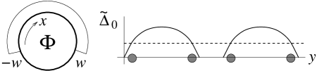
Figure 1: (Left) Cross section of a SC contact deposited on the surface of a TI nanocylinder. The TI surface is shown by a thicker line. (Right) Proximity-induced pairing amplitude modulus in the TI, as a function of the longitudinal coordinate, for the case when two such contacts are present. The dashed horizontal line represents the value $\delta(\Phi)$ (defined in the text) for some longitudinal flux $\Phi$. As $\Phi$ changes, $\delta(\Phi)$ sweeps through the range of $\tilde{\Delta}_{0}$. The points where it intersects $\tilde{\Delta}_{0}(y)$ are locations of MBSs (shaded circles).

Because this system presents a potentially useful alternative to a planar SQUID, and to underscore the generality of the trapping mechanism, let us briefly describe the argument for the existence of MBSs in it (full details will be published elsewhere SK:elsewhere ). The argument is based on the Hamiltonian of Fu and Kane Fu&Kane adapted to a cylindrical surface Zhang&al and coupled to an external vector potential ${\cal A}_{x}$.

Unlike Refs. Cook&Franz ; Ilan&al , we do not assume that the proximity-induced pairing amplitude $\Delta(x,y)$ in the Hamiltonian of the TI surface states extends over the entire circumference. Rather, each contact has a break, in which $\Delta(x,y)=0$. The break turns each contact into a quantum interferometer, which can be controlled by the longitudinal magnetic flux $\Phi$.

Suppose the SC layer is thick enough to lock the phase of $\Delta$ to ${\cal A}_{x}$, that is

$$\Delta(x,y)=\tilde{\Delta}(x,y)\mbox{e}^{-2ie{\cal A}_{x}x}\,,$$ (1)

where $\tilde{\Delta}\geq 0$ is real; $e>0$ in the exponent is the magnitude of the electron charge. ${\cal A}_{x}$ has been made $x$-independent by a gauge choice, so that $\Phi={\cal A}_{x}L_{x}$, where $L_{x}$ is the circumference. Note that, for a general ${\cal A}_{x}$, the state (1) is possible only because the phase of $\Delta$ is not restricted by periodicity in $x$. That would not be so in the absence of a break in the SC layer.

The simplest case is when the chemical potential $\mu$ is a constant, while $\tilde{\Delta}(x,y)$ is a slowly varying function of $y$, $\tilde{\Delta}(x,y)=\tilde{\Delta}_{0}(y)$, for $-w<x<w$ and zero otherwise (here we consider the version in which $w$ is independent of $y$). In this case, we can at first neglect $\partial_{y}$ in the Fu-Kane Hamiltonian. We then find that, for any $\Phi$ in a certain range, there is a value $\tilde{\Delta}_{0}=\delta(\Phi)$ at which the Hamiltonian has zero-energy states. With $\partial_{y}$ reinstated, intersections of $\tilde{\Delta}_{0}(y)$ with $\delta(\Phi)$ become locations of MBSs (see Fig. 1). As $\Phi$ changes between 0 and $\Phi_{0}=\pi\hbar/e$ (the superconducting flux quantum), these MBSs are produced, travel, and disappear, as the intersection points would. If $\tilde{\Delta}_{0}(y)$ is not slowly varying, stability of an isolated MBS can be argued by using a mod 2 index, similarly to the argument in the discussion of global anomaly in Ref. Witten:1982 .

In trapping by modulus, as in trapping by phase Fu&Kane , the low-energy theory of the MBSs is based on the one-dimensional (if we only count the spatial dimensions) Dirac equation, with the additional “reality” restriction on the fermion. One can show that this low-energy theory applies also to SC-semiconductor wire hybrids, proposed as a platform for MBSs in Refs. Lutchyn&al ; Oreg&al , so our results hold for that case as well. The MBSs are trapped by the mechanism of Jackiw&Rebbi on “kinks”—simple zeroes of the fermion mass term.

Here, we would like to address one particular aspect of the physics of that low-energy theory. The energy of two well-separated MBSs is exponentially small for large separations. So, in a long enough device, the process described above can be viewed as a passage through an anti-crossing of two or more exponentially close energy levels. If the process is adiabatic on the scale of the typical quasiparticle energy but not on the scale of the exponentially small level spacing of the MBSs, one may ask if there is a version of the Landau-Zener (LZ) effect, namely, a significant probability of transition from the ground to an excited state.

The difference between the present case and the standard LZ case LL is two-fold. First, there is a difference in the language of description. The Fermi statistics is best described by second quantization, so the natural language to discuss the process in our case is that of particle production by a time-dependent external field. If the system starts in the ground state with no MBSs, then goes through production, transport, and annihilation of those—so that none are left in the final state—it will in general end in a linear combination of the ground state and states containing quasiparticles. Using the formalism of in- and out-states, we can write this as

$$|0_{in}\rangle=f_{0}|0_{out}\rangle+f_{2}b^{\dagger}c^{\dagger}|0_{out}\rangle+\ldots\,,$$ (2)

where $b^{\dagger}$ and $c^{\dagger}$ are quasiparticle creation operators, and $f_{0}$, $f_{2}$ are the transition amplitudes. Note that even in the simplest case (when the additional terms indicated by $\ldots$ are absent), the process requires participation of at least two quasiparticle modes (corresponding to the two operators in (2)). A pair of MBSs gives rise to a single excitation mode, so we conclude that the minimal setup in which a non-trivial effect is possible is that involving four MBSs.

The second difference between our problem and the original LZ calculation is that the latter applies to a specific form of anti-crossing of levels, namely, an avoided crossing of two straight lines. That form is generic when the off-diagonal elements of the $2\times 2$ reduced Hamiltonian are approximately constant at the crossing point, while the diagonal terms have simple zeroes. In our case, however, the matrix elements do not have this structure: if one were to neglect the overlap between the MBSs, their energies would be zero identically.

One may compare the effect described here to transitions induced by a change of the phase difference between the ends of a proximity-coupled wire that supports two MBSs at the ends Kitaev or to LZ transitions induced by a phase sweep in a wire that supports four MBSs—two at the ends and two more in the middle San-Jose&al ; Pikulin&Nazarov ; Dominguez&al . The difference is that, in either of those cases, the MBSs exist permanently, while in our case they are only present during the intermediate stages. Note in this connection that the avoided crossing considered in Refs. San-Jose&al ; Pikulin&Nazarov ; Dominguez&al is of the conventional straight-line type.

Here, we describe a computation of the LZ effect—or, equivalently, particle production—in the setting corresponding to Fig. 1, defined in particular by the absence of MBSs in the initial and final states and by exponential crossing of the levels. We consider the minimal case identified above: two kink-anti-kink pairs, the relative positions (and existence) of the kinks and antikinks being controlled by a single parameter, the separation $a$. The computation is done within the 4-dimensional subspace comprised of the first-quantized fermion states with energies closest to zero. We construct the $4\times 4$ $S$-matrix for these states by numerically solving the evolution equations and then convert it into a second-quantization relation of the form (2).

We find that a pair of quasiparticles is produced with probability 50%, i.e., $f_{2}=f_{0}=1/\sqrt{2}$ (with no additional terms present). This result has a curious degree of universality: as far as we can tell, it applies regardless of the detailed form of the wavefunctions, as long as the conditions of adiabaticity (as defined above) and presence of well-separated MBSs during the intermediate stage are intact. With these values of $f_{0}$ and $f_{2}$, Eq. (2) becomes equivalent to a fusion rule for non-Abelian anyons in the two-dimensional model of Ref. Kitaev:2006 . That rule has been predicted to hold also for MBSs localized on triple junctions in a TI-based JJ circuit Fu&Kane . One implication of the universal nonzero value of $f_{2}$ is that any novel technology that aims to manipulate MBSs will have to contend with the possibility of quasiparticle production and its associated effects (decoherence, heating, etc.).

Experimental verification of Eq. (2) for the system of Fig. 1 is possible along the lines proposed for the planar circuit in Ref. Fu&Kane (and adapted to nanowires in Ref. Alicea&al ). Namely, a measurement of the Josephson current between the contacts will produce one of two different values, depending on which component of the linear superposition is projected out, with 50% probability for each.

Our starting point then is the (1+1)-dimensional Dirac equation with a $y$-dependent mass ($y$ is the coordinate along the single spatial dimension):

$$i\partial_{t}\Psi=[-i\sigma_{y}\partial_{y}+M(y)\sigma_{z}]\Psi\equiv{\cal H}_{2}\Psi\,.$$ (3)

Here $\Psi$ is a two-component fermion operator, and $\sigma$ are the Pauli matrices. (We set both $\hbar$ and the velocity parameter to 1.) The first-quantized Hamiltonian ${\cal H}_{2}$ defined in (3) has a particle-hole symmetry: if

$$V_{n}(y)=[A_{n}(y),B_{n}(y)]^{T}$$ (4)

is an eigenstate of ${\cal H}_{2}$ with energy $E_{n}$, then

$$V^{\prime}_{n}(y)=[B_{n}(y),A_{n}(y)]^{T}$$ (5)

is also an eigenstate, with energy $-E_{n}$. Because ${\cal H}_{2}$ is real, we can choose both $A_{n}$ and $B_{n}$ to be real as well.

The Majorana case occurs when the components of $\Psi$ are constrained to be Hermitian conjugate of each other:

$$\Psi=(\psi,\psi^{\dagger})^{T}\,.$$ (6)

In this case, the operator solution to (3) is

$$\Psi(y,t)={\sum_{n}}^{\prime}[a_{n}V_{n}(y)e^{-iE_{n}t}+a_{n}^{\dagger}V_{n}^{\prime}(y)e^{iE_{n}t}]\,,$$ (7)

where $a_{n}$, $a_{n}^{\dagger}$ are fermionic annihilation and creation operators, and the prime on the sum indicates that each pair of states $V_{n},V^{\prime}_{n}$ related by the particle-hole symmetry is included only once; in particular, $E_{n}\geq 0$.

A single simple zero of $M(y)$ (a “kink”) in the infinite system would be a location of a Jackiw-Rebbi bound state Jackiw&Rebbi , for which $E_{n}=0$ and $V_{n}=V_{n}^{\prime}$ up to a sign. Substituting this into (7) we see that both components of $\Psi$ are expressed through a single Hermitian linear combination of $a_{n}$ and $a_{n}^{\dagger}$, a Majorana fermion. Motivated by realistic examples, for which (3) is the low-energy limit, we consider instead the case when $M(y)$ has an even number of kinks, which can be produced and destroyed in pairs by variations of $M(y)$. In this case, there are no strictly vanishing $E_{n}$ but, when all the kinks are well separated, there are some exponentially small $E_{n}>0$, one for each pair of kinks.

Next, we review the origin of LZ transitions. Suppose a first-quantized Hamiltonian ${\cal H}$ depends slowly on time, and there are two or more eigenstates $V_{n}(t)$ of the instantaneous ${\cal H}(t)$ whose energies, $E_{n}(t)$, undergo an avoided crossing. To the extent we can restrict the time evolution to the subspace spanned by these eigenstates, we can search for a solution to the full time-dependent Schrödinger equation (SE) $i\partial_{t}\Psi(t)={\cal H}(t)\Psi(t)$ in the form

$$\Psi(t)=\sum_{n}c_{n}(t)V_{n}(t)e^{-i\int^{t}E_{n}dt^{\prime}}\,.$$ (8)

Projecting the SE back onto the subspace, one obtains evolution equations for the coefficients $c_{n}$. If, as in the present case, the eigenfunctions are real, these equations simplify into

$$\partial_{t}c_{m}+\sum_{n\neq m}e^{i\int^{t}\Delta E_{mn}dt^{\prime}}\Pi_{mn}(t)c_{n}=0\,,$$ (9)

where $\Delta E_{mn}(t)=E_{m}(t)-E_{n}(t)$, and

$$\Pi_{mn}(t)=-\Pi_{nm}(t)=\langle V_{m}|\partial_{t}V_{n}\rangle\,.$$ (10)

Two limiting cases can be considered. When a $\Pi_{mn}(t)$ varies slowly compared to the phase factor accompanying it in the equations, even a large $\Pi_{mn}(t)$ will be ineffective; this is the adiabatic limit. In the opposite limit, of interest to us here, all $\Delta E_{mn}$ can be neglected during the entire time when $\Pi_{mn}$ are operational. Then, probabilities of transition between different $V_{n}$ are determined solely by $\Pi_{mn}(t)$.

Note that in the latter limit, if ${\cal H}$ depends on time through a dependence on a parameter $a$, time can be removed from the equations entirely, by replacing $\partial_{t}$ with $\partial_{a}$ in both (9) and (10). In other words, the precise form of the $a(t)$ dependence does not matter (as long as the conditions allowing the use of the limit are satisfied). In the original LZ case, corresponding to an anti-crossing of two levels represented by straight lines, the probability of the transition in this limit approaches unity LL . For the present case, it must be computed anew.

The case of four states (with real wavefunctions) involves four time-dependent coefficients, $c_{0}$ through $c_{3}$, and six distinct matrix elements $\Pi_{mn}$ of the form (10). We consider four eigenstates of ${\cal H}_{2}$, Eq. (3), with energies closest to zero and label them in the order of increasing energy, so that the particle-hole symmetry relates $V_{0}$ (the lowest-energy state of the four) to $V_{3}$, and $V_{1}$ to $V_{2}$. In our earlier notation, this means that $V_{0}=V_{3}^{\prime}$ and $V_{1}=V_{2}^{\prime}$. In the limit when all the energy differences are small (in the above-stated sense), the evolution equations become

$$\partial_{t}c_{m}+\sum_{n\neq m}\Pi_{mn}(t)c_{n}=0\,,$$ (11)

where $m,n=0,\ldots,3$.

We have obtained the eigenstates $V_{n}$ required for computation of $\Pi_{mn}$ by discretization of (3) on a one-dimensional grid and numerical diagonalization. The fermions are assumed to obey antiperiodic boundary conditions on the segment $0\leq y\leq L_{y}$. In the continuum limit, we aim for $M(y)=\phi(y)$, where $\phi(y)$ is composed of kinks and antikinks at positions $y_{a}=y_{L}-a$, $y_{b}=y_{L}+a$, $y_{c}=y_{R}-a$, and $y_{d}=y_{R}+a$, as follows:

$$\phi(y)=\phi_{0}\left[-1+K(y-y_{a},\xi_{L})-K(y-y_{b},\xi_{L})\right.$$

$$\left.{}+K(y-y_{c},\xi_{R})-K(y-y_{d},\xi_{R})\right]\,,$$ (12)

where

$$K(y,\xi)=\tanh(y/\xi)$$ (13)

is the kink, and $-K$ is the antikink; $\phi_{0}>0$ is a constant. (In the discrete version, it is convenient to deviate somewhat from $M(y)=\phi(y)$ in order to better preserve the continuum form of the MBS wavefunctions.)

In each simulation, we pick specific values of the parameters $\phi_{0},y_{L},y_{R},\xi_{L},\xi_{R}$ and vary $a$, the remaining parameter, which controls the kink-antikink separation. When $a=0$, we have $\phi=-\phi_{0}$, a uniform state without kinks or MBSs. As $a$ increases from zero, a kink-antikink pair appears at $y=y_{L}$ and another at $y=y_{R}$. At large enough $a$, two kinks disappear through the ends of the segment, and two annihilate in the middle. So, they travel exactly as the intersection points in Fig. 1 do when the horizontal line sweeps through the range of $\tilde{\Delta}_{0}$ from top to bottom. We choose $y_{L}$ and $y_{R}$ to be closer to the middle of the segment than to the ends, so the kinks heading towards the middle disappear first.

Fig. 2 shows the result of a numerical integration of (11) with the initial condition $c_{0}=1$, $c_{n}=0$ for $n>0$ for a particular choice of the parameters, together with the behavior of the four levels in question. We see a nontrivial evolution of $c_{n}$ during the time all the four levels are close to one another. Note that at the largest value of $a$ shown, there are still two MBSs, corresponding to a kink and an antikink near the ends of the interval. Their motion, however, does not produce any further change in $c_{n}$, confirming the expectation that the minimum of four MBSs is required for a nontrivial effect. (That can also be verified in a simulation in which only two MBSs are produced from the start.)

Figure 2: Evolution of the coefficients $c_{n}$ (solid lines), obtained by numerical integration of Eq. (11) for $\phi_{0}=5$, $y_{L}=3$, $y_{R}=7$, $\xi_{L}=0.4$, $\xi_{R}=0.2$, $L_{y}=10$, together with the corresponding eigenvalues of the instantaneous ${\cal H}_{2}(a)$ (dashed lines).

Let us combine the four $c_{n}$ into a column

$$C=(c_{0},c_{1},c_{2},c_{3})^{T}$$ (14)

and refer to the asymptotics of $C$ at small and large $a$ as $C_{in}$ and $C_{out}$, respectively. We can then define a $4\times 4$ $S$-matrix connecting these asymptotics,

$$C_{out}=\hat{S}C_{in}\,.$$ (15)

Numerically, we find

$$\hat{S}=\left(\begin{array}[]{cccc}\frac{1}{2}&-\frac{1}{2}&\frac{1}{2}&\frac{1}{2}\\ \frac{1}{2}&\frac{1}{2}&\frac{1}{2}&-\frac{1}{2}\\ -\frac{1}{2}&\frac{1}{2}&\frac{1}{2}&\frac{1}{2}\\ \frac{1}{2}&\frac{1}{2}&-\frac{1}{2}&\frac{1}{2}\end{array}\right)$$ (16)

(For instance, the first column of this can be read off Fig. 2.) We find this result to be quite generic, i.e., equivalent $S$-matrices are obtained for different values of the parameters (provided four well-separated MBSs occur in the intermediate state).

To go over to second quantization, we replace the components of $C_{in}$ and $C_{out}$ with two sets of creation and annihilation operators, as follows:

$$C_{in} = (a_{3}^{\dagger},a_{2}^{\dagger},a_{2},a_{3})^{T}\,,$$ (17)

$$C_{out} = (b_{3}^{\dagger},b_{2}^{\dagger},b_{2},b_{3})^{T}\,.$$ (18)

Note that, as prescribed by (7), we associate annihilation operators with the positive energy exponentials, and creation operators with the negative energy ones. Eq. (15) becomes a Bogoliubov transformation relating the two sets.

Suppose the system is in the in-vacuum, defined by the conditions

$$a_{2}|0_{in}\rangle=a_{3}|0_{in}\rangle=0\,.$$ (19)

We wish to express $|0_{in}\rangle$ through the out-states, in particular, the out-vacuum, defined by

$$b_{2}|0_{out}\rangle=b_{3}|0_{out}\rangle=0\,.$$ (20)

Inverting (15), we find

$$a_{2} = \frac{1}{2}(b_{3}^{\dagger}+b_{2}^{\dagger}+b_{2}-b_{3})\,,$$ (21)

$$a_{3} = \frac{1}{2}(b_{3}^{\dagger}-b_{2}^{\dagger}+b_{2}+b_{3})\,.$$ (22)

The solution to (19) then is

$$|0_{in}\rangle=\frac{1}{\sqrt{2}}(1-b_{2}^{\dagger}b_{3}^{\dagger})|0_{out}\rangle\,,$$ (23)

which shows that there is a 50% probability to produce a quasiparticle pair.

The configuration (12) describes annihilation of counter-propagating kinks that have been produced (in pairs) at two different locations, $y_{L}$ and $y_{R}$. One may also consider the case when two pairs appear at the same point (say, the middle of the interval) at different times, and the kink from one pair eventually catches up with the antikink from the other. (This can occur, for instance, for Josephson vortices in a planar SQUID that contains a long junction of the type considered in Ref. Potter&Fu .) We have found that the $S$-matrix for that case is equivalent to (16), so the probability of quasiparticle production is again 50%.

- (1) L. Fu and C. L. Kane, Phys. Rev. Lett. 100, 096407 (2008).
- (2) P. A. Ioselevich and M. V. Feigel’man, Phys. Rev. Lett. 106, 077003 (2011).
- (3) A. Cook and M. Franz, Phys. Rev B 84, 201105(R) (2011).
- (4) R. Ilan, J. H. Bardarson, H.-S. Sim, and J. E. Moore, New J. Phys. 16, 053007 (2014).
- (5) R. Jackiw and C. Rebbi, Phys. Rev. D 13, 3398 (1976).
- (6) A. C. Potter and L. Fu, Phys. Rev. B 88, 121109(R) (2013).
- (7) M. Kayyalha et al., eprint arXiv:1712.02748.
- (8) S. Khlebnikov, to be published.
- (9) Y. Zhang, Y. Ran, and A. Vishwanath, Phys. Rev B 79, 245331 (2009).
- (10) E. Witten, Phys. Lett. 117B, 324 (1982).
- (11) R. M. Lutchyn, J. D. Sau, and S. Das Sarma, Phys. Rev. Lett. 105, 077001 (2010).
- (12) Y. Oreg, G. Refael, and F. von Oppen, Phys. Rev. Lett. 105, 177002 (2010).
- (13) L. D. Landau and E. M. Lifshitz, Quantum Mechanics. Nonrelativistic Theory, 3rd ed. (Nauka, Moscow, 1974), Sec. 90.
- (14) A. Yu. Kitaev, Physics-Uspekhi 44, 131 (2001).
- (15) P. San-Jose, E. Prada, and R. Aguado, Phys. Rev. Lett. 108, 257001 (2012).
- (16) D. I. Pikulin and Y. V. Nazarov, Phys. Rev. B 86, 140504(R) (2012).
- (17) F. Domínguez, F. Hassler, and G. Platero, Phys. Rev. B 86, 140503(R) (2012).
- (18) A. Kitaev, Annals of Physics 321, 2 (2006).
- (19) J. Alicea, Y. Oreg, G. Refael, F. von Oppen, and M. P. A. Fisher, Nature Physics 7, 412 (2011).