The HOMFLY-PT polynomial is fixed-parameter tractable

Abstract.

Many polynomial invariants of knots and links, including the Jones and HOMFLY-PT polynomials, are widely used in practice but #P-hard to compute. It was shown by Makowsky in 2001 that computing the Jones polynomial is fixed-parameter tractable in the treewidth of the link diagram, but the parameterised complexity of the more powerful HOMFLY-PT polynomial remained an open problem. Here we show that computing HOMFLY-PT is fixed-parameter tractable in the treewidth, and we give the first sub-exponential time algorithm to compute it for arbitrary links.

1. Introduction

In knot theory, polynomial invariants are widely used to distinguish between different topological knots and links. Although they are powerful tools, these invariants are often difficult to compute: in particular, the one-variable Jones polynomial [10] and the stronger two-variable HOMFLY-PT polynomial [7, 19] are both #P-hard to compute in general [8, 20].

Despite this, we can use parameterised complexity to analyse classes of knots and links for which these polynomials become tractable to compute. In the early 2000s, as a part of a larger work on graph polynomials, Makowsky showed that the Jones polynomial can be computed in polynomial time for links whose underlying 4-valent graphs have bounded treewidth [15]—in other words, the Jones polynomial is fixed-parameter tractable with respect to treewidth. A slew of other parameterised tractability results also appeared around this period for the Jones and HOMFLY-PT polynomials: parameters included the pathwidth of the underlying graph [16], the number of Seifert circles [16, 17], and the complexity of tangles in an algebraic presentation [16].

However, there was an important gap: it remained open as to whether the HOMFLY-PT polynomial is fixed-parameter tractable with respect to treewidth. This was dissatisfying because the HOMFLY-PT polynomial is both powerful and widely used, and the treewidth parameter lends itself extremely well to building fixed-parameter tractable algorithms, due to its strong connections to logic [4, 5] and its natural fit with dynamic programming.

The first major contribution of this paper is to resolve this open problem: we prove that computing the HOMFLY-PT polynomial of a link is fixed-parameter tractable with respect to treewidth (Theorem 8). Our proof gives an explicit algorithm; this is feasible to implement, and will soon be released as part of the topological software package Regina [1, 2].

Regarding practicality: fixed-parameter tractable algorithms are only useful if the parameter is often small, and in this sense treewidth is a useful parameter: the underlying graph is planar, and so the treewidth of an $n$-crossing link diagram is at worst $O(\sqrt{n})$. This is borne out in practice—for instance, a simple greedy computation using Regina shows that, for Haken’s famous 141-crossing “Gordian unknot”, the treewidth is at most 12. Since HOMFLY-PT is a topological invariant, one can also attempt to use local moves on a link diagram to reduce the treewidth of the underlying graph, and Regina contains facilities for this also.

There are few explicit algorithms in the literature for computing the HOMFLY-PT polynomial in general: arguably the most notable general algorithm is Kauffman’s exponential-time skein-template algorithm [11], which forms the basis for our algorithm in this paper. Other notable algorithms are either designed for specialised inputs (e.g., Murakami et al.’s algorithm for 2-bridge links [18]), or are practical but do not prove unqualified guarantees on their complexity [3, 9].

The second major contribution of this paper is to improve the worst-case running time for computing the HOMFLY-PT polynomial in the general case—in particular, we prove the first sub-exponential running time (Corollary 21). Here by subexponential we mean $e^{o(n)}$; the specific bound that we give is $e^{O(\sqrt{n}\cdot\log n)}$. The result follows immediately from analysing our fixed-parameter tractable algorithm using the $O(\sqrt{n})$ bound on the treewidth of a planar graph.

Throughout this paper we assume that the input link diagram contains no zero-crossing components (i.e., unknotted circles that are disjoint from the rest of the link diagram), since otherwise the number of crossings is not enough to adequately measure the input size. Such components are easy to handle—each zero-crossing component multiplies the HOMFLY-PT polynomial by $(\alpha-\alpha^{-1})z^{-1}$, and so we simply compute the HOMFLY-PT polynomial without them and then adjust the result accordingly.

2. Background

A link is a disjoint union of piecewise linear closed curves embedded in $\mathbb{R}^{3}$; the image of each curve is a component of the link. A knot is a link with precisely one component. In this paper we orient our links by assigning a direction to each component.

A link diagram is a piecewise linear projection of a link onto the plane, where the only multiple points are crossings at which one section of the link crosses another transversely. The sections of of the link diagram between crossings are called arcs. The number of crossings is often used as a measure of input size; in particular, an $n$-crossing link diagram can be encoded in $O(n\log n)$ bits without losing any topological information.

Figure 1 shows two examples: the first is a knot with 4 crossings and 8 arcs, and the second is a 2-component link with 5 crossings and 10 arcs.

Figure 1. Examples of knots and links

Each crossing has a sign which is either positive or negative, according to the direction in which the upper strand passes over the lower; see Figure 2 for details. The writhe of a link diagram is the number of positive crossings minus the number of negative crossings (so the examples from Figure 1 have writhes 0 and $-1$ respectively).

Figure 2. Positive and negative crossings

In this paper we use two operations that change a link diagram at a single crossing. To switch a crossing is to move the upper strand beneath the lower, and to splice a crossing is to change the connections between the incoming and outgoing arcs; see Figure 3.

Figure 3. Switching and splicing a crossing

The HOMFLY-PT polynomial of a link $\mathcal{L}$ is a Laurent polynomial in the two variables $\alpha$ and $z$ (a Laurent polynomial is a polynomial that allows both positive and negative exponents). There are two different but essentially equivalent definitions of the HOMFLY-PT polynomial in the literature (the other is typically given as a polynomial in $\ell$ and $m$ [13]); we follow the same definition used by Kauffman [11].

A parameterised problem is a computational problem where the input includes some numerical parameter $k$. Such a problem is said to be fixed-parameter tractable if there is an algorithm with running time $O(f(k)\cdot\mathrm{poly}(n))$, where $f$ is an arbitrary function and $n$ is the input size. A consequence of this is that, for any class of inputs whose parameter $k$ is universally bounded, the algorithm runs in polynomial time.

Treewidth is a common parameter for fixed-parameter tractable algorithms on graphs, and we discuss it in detail now. Throughout this paper, all graphs are allowed to be multigraphs; that is, they may contain parallel edges and/or loops.

Definition 1 (Treewidth).

Given a graph $\Gamma$ with vertex set $V$, a tree decomposition of $\Gamma$ consists of a tree $\tau$ and bags $\beta_{i}\subseteq V$ for each node $i$ of $T$, subject to the following constraints: (i) each $v\in V$ belongs to some bag $\beta_{i}$; (ii) for each edge of $\Gamma$, its two endpoints $v,w\in V$ belong to some common bag $\beta_{i}$; and (iii) for each $v\in V$, the bags containing $v$ correspond to a (connected) subtree of $T$.

The width of this tree decomposition is $\max|\beta_{i}|-1$, and the treewidth of $\Gamma$ is the smallest width of any tree decomposition of $\Gamma$.

A consequence of the Lipton-Tarjan planar separator theorem [14] is that every planar graph on $n$ vertices has treewidth $O(\sqrt{n})$.

Definition 2 (Rooted tree decomposition).

Let $\Gamma$ be a graph. A rooted tree decomposition of $\Gamma$ is a tree decomposition where one bag is singled out as the root bag. We define children and parents in the usual way: for any adjacent bags $\beta,\beta^{\prime}$ in the tree, if $\beta$ is closer in the tree to the root than $\beta^{\prime}$ then we call $\beta^{\prime}$ a child bag of $\beta$, and we call $\beta$ the (unique) parent bag of $\beta^{\prime}$. A bag with no children is called a leaf bag.

More generally, we say that bag $\beta^{\prime}$ is a descendant of bag $\beta$ if $\beta\neq\beta^{\prime}$ and there is some sequence $\beta=\beta_{0},\beta_{1},\beta_{2},\ldots,\beta_{i}=\beta^{\prime}$ where each $\beta_{i}$ is the parent bag of $\beta_{i+1}$.

Definition 3 (Nice tree decomposition).

Let $\Gamma$ be a graph. A nice tree decomposition of $\Gamma$ is a rooted tree decomposition with the following additional properties:

1. The root bag is empty.

2. Every leaf bag contains precisely one vertex.

3. Every non-leaf bag has either one or two child bags.

4. If a bag $\beta_{i}$ has two child bags $\beta_{j}$ and $\beta_{k}$, then $\beta_{i}=\beta_{j}=\beta_{k}$; we call $\beta_{i}$ a join bag.

5. If a bag $\beta_{i}$ has only one child bag $\beta_{j}$, then either:

   • $|\beta_{i}|=|\beta_{j}|+1$ and $\beta_{i}\supset\beta_{j}$. Here we call $\beta_{i}$ an introduce bag, and the single vertex in $\beta_{i}\backslash\beta_{j}$ is called the introduced vertex.

   • $|\beta_{i}|=|\beta_{j}|-1$ and $\beta_{i}\subset\beta_{j}$. Here we call $\beta_{i}$ a forget bag, and the single vertex in $\beta_{j}\backslash\beta_{i}$ is called the forgotten vertex.

3. Kauffman’s skein-template algorithm

Kauffman’s skein-template algorithm works by building a decision tree. The leaves of this decision tree are obtained from the original link by switching and/or splicing some crossings. Each leaf is then evaluated as a Laurent polynomial, according to the number of components and the specific switches and/or splices that were performed, and these are summed to obtain the final HOMFLY-PT polynomial.

Our fixed-parameter tractable algorithm (described in Section 4) works by inductively constructing, aggregating and analysing small pieces of Kauffman’s decision tree. We therefore devote this section to describing Kauffman’s algorithm in detail, beginning with a description of the algorithm itself followed by a detailed example.

Algorithm 4 (Kauffman [11]).

Let $\mathcal{L}$ be a link diagram with $n$ crossings (and therefore $2n$ arcs). Then the following procedure computes the HOMFLY-PT polynomial of $\mathcal{L}$.

Arbitrarily label the arcs $1,2,\ldots,2n$. We build a decision tree by walking through the link as follows:

• Locate the lowest-numbered arc that has not yet been traversed, and follow the link along this arc in the direction of its orientation.

• Each time we encounter a new crossing that has not yet been traversed:

  • If we are passing over the crossing, then we simply pass through it and continue traversing the link.

  • If we are passing under the crossing, then we make a fork in the decision tree. On one branch we splice the crossing, and on the other branch we switch the crossing. Either way, we then pass through the crossing (following the splice if we made one) and continue traversing the link.

• Whenever we encounter a crossing for the second time, we simply pass through it (again following the splice if we made one) and continue traversing the link.

• Whenever we return to an arc that has already been traversed (thus closing off a component of our modified link):

  • If there are still arcs remaining that have not yet been traversed, then we locate the lowest-numbered such arc and continue our traversal from there.

  • If every arc has now been traversed, then the resulting modified link becomes a leaf of our decision tree.

To each leaf of the decision tree, we assign the polynomial term $(-1)^{t_{-}}z^{t}\alpha^{w-w_{0}}\delta^{c-1}$, where:

• $t$ is the number of splices that we performed on this branch of the decision tree;

• $t_{-}$ is the number of splices that we performed on negative crossings;

• $w$ is the writhe of the modified link, after any switching and/or splicing;

• $w_{0}$ is the writhe of the original link $\mathcal{L}$, before any switching or splicing;

• $c$ is the number of components of the modified link;

• $\delta$ expands to the polynomial $(\alpha-\alpha^{-1})z^{-1}$.

The HOMFLY-PT polynomial of $\mathcal{L}$ is then the sum of these polynomial terms over all leaves.

Note that different branches of the decision tree may traverse the arcs of the link in a different order, since each splice changes the connections between arcs; likewise, the modified links at the leaves of the decision tree may have different numbers of link components.

Example 5.

Figure 4 shows the algorithm applied to the figure eight knot, as depicted at the root of the tree. The eight arcs are numbered 1–8; to help with the discussion we also label the four crossings $A$, $B$, $C$ and $D$, which have signs $+$, $-$, $-$ and $+$ respectively.

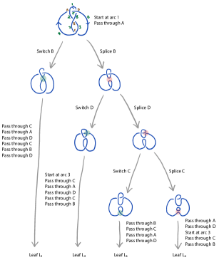
Figure 4. Running Kauffman’s skein-template algorithm

We begin at arc 1, and because we first encounter crossing $A$ on the upper strand, we leave it unchanged and move on to arc 2. For crossing $B$ we can either switch or splice, and in these cases the traversal continues to arc 3 or 8 respectively. The decision process continues as shown in the diagram, resulting in the four leaves $L_{1}$, $L_{2}$, $L_{3}$ and $L_{4}$.

Of particular note is the branch where we splice $B$ and then switch $D$. Here the traversal runs through arcs 1, 2 and 8, at which point it returns to arc 1, closing off a small loop. We now begin again at arc 3: this takes us through crossing $C$ (which we pass through because we see it first on the upper strand), then crossing $A$ (which we pass through because we are seeing it for the second time), then crossing $D$ (which we likewise pass through), and so on.

The polynomials assigned to the four leaves are shown below:

$$\small\begin{array}[]{l|r|r|r|r|r|c}&t&t_{-}&w&w-w_{0}&c&\mbox{Poly.}\\ \hline\cr L_{1}&0&0&2&2&1&\alpha^{2}\\ L_{2}&1&1&-1&-1&2&-z\alpha^{-1}\delta\\ \end{array}\qquad\begin{array}[]{l|r|r|r|r|r|c}&t&t_{-}&w&w-w_{0}&c&\mbox{Poly.}\\ \hline\cr L_{3}&2&1&2&2&1&-z^{2}\alpha^{2}\\ L_{4}&3&2&1&1&2&z^{3}\alpha\delta\end{array}$$

This yields the final HOMFLY-PT polynomial

$$\alpha^{2}-z^{2}\alpha^{2}+(z^{3}\alpha-z\alpha^{-1})\delta=\alpha^{2}-z^{2}\alpha^{2}+(z^{3}\alpha-z\alpha^{-1})(\alpha-\alpha^{-1})z^{-1}=\alpha^{2}+\alpha^{-2}-z^{2}-1.$$

Assumptions 6.

Kauffman’s skein-template algorithm computes the HOMFLY-PT polynomial of an $n$-crossing link in time $2^{n}\cdot\mathrm{poly}(n)$.

Proof.

The decision tree has $\leq 2^{n}$ leaves, since we only branch the first time we traverse each crossing (and even then, only if we first traverse the crossing from beneath, not above). All other operations are polynomial time, giving an overall running time of $2^{n}\cdot\mathrm{poly}(n)$ ∎

Although it requires exponential time, Kauffman’s algorithm can compute the HOMFLY-PT polynomial in polynomial space. This is because we do not need to store the entire decision tree—we can simply perform a depth-first traversal through the tree, making and undoing switches and splices as we go, and keep a running total of the polynomial terms for those leaves that we have encountered so far.

4. A fixed-parameter tractable algorithm

In this section we present an explicit algorithm to show that computing the HOMFLY-PT polynomial is fixed-parameter tractable in the treewidth of the input link diagram.

Definition 7.

Let $\mathcal{L}$ be a link diagram. The graph of $\mathcal{L}$, denoted $\Gamma(\mathcal{L})$, is the directed planar 4-valent multigraph whose vertices are the crossings of $\mathcal{L}$, and whose directed edges are the oriented arcs of $\mathcal{L}$.

The first main result of this section, which resolves the open problem of the parameterised complexity of computing the HOMFLY-PT polynomial, is:

Assumptions 8.

Consider the parameterised problem whose input is a link diagram $\mathcal{L}$, whose parameter is the treewidth of the graph $\Gamma(\mathcal{L})$, and whose output is the HOMFLY-PT polynomial of $\mathcal{L}$. Then this problem is fixed-parameter tractable.

4.1. Algorithm overview

The remainder of Section 4 is devoted to proving Theorem 8. First, however, we give a brief overview of the algorithm and the difficulties that it must overcome.

Roughly speaking, our algorithm takes a nice tree decomposition of $\Gamma(\mathcal{L})$ and works from the leaf bags to the root bag. For each bag of the tree, we consider a range of possible “boundary conditions” for how a link traversal interacts with the bag, and for each set of boundary conditions we aggregate all “partial leaves” of Kauffman’s decision tree that satisfy them. We formalise these boundary conditions and their resulting aggregations using the notions of a configuration and evaluation respectively (Definitions 12 and 16).

This general pattern of dynamic programming over a tree decomposition is common for fixed-parameter tractable algorithms. The main difficulty that we must overcome is to keep the number of configurations polynomial in the number of crossings $n$. This difficulty arises because the choices in Kauffman’s decision tree depend upon the order in which you traverse the crossings, and so each configuration must encode a starting arc for every section of a link traversal in every “partial leaf” of the decision tree. Because a “partial leaf” could contain $O(n)$ disjoint sections of a traversal, each with $O(n)$ potential starting arcs, the resulting number of configurations would grow at a rate of $O(n^{n})$, which is too large.

Our solution is the following. Recall that Kauffman’s algorithm uses an arbitrary ordering of the arcs of the link to determine the order in which we traverse arcs and make decisions (to pass through, switch and/or splice crossings). In our algorithm, we order the arcs using the tree decomposition—for each directed arc, we identify the forget bag in which its end crossing is forgotten, and we then order the arcs according to how close this forget bag is to the root of the tree. This makes the ordering of arcs inherent to the tree decomposition, and so we do not need to explicitly encode starting arcs in our configurations. This is enough to reduce the number of configurations at each bag to a function of the treewidth alone, with no dependency on $n$.

4.2. Properties of tree decompositions

We now make some small observations about tree decompositions of the graphs of links.

Definition 9.

Let $\mathcal{L}$ be a link diagram, let $T$ be a rooted tree decomposition of $\Gamma(\mathcal{L})$, and let $\beta$ be any bag of $T$. For each crossing $c$ of $\mathcal{L}$, we say that:

• $c$ is unvisited at $\beta$ if $c$ does not appear in either $\beta$ or any bags in the subtree rooted at $\beta$;

• $c$ is current at $\beta$ if $c$ appears in the bag $\beta$ itself;

• $c$ is forgotten at $\beta$ if $c$ does not appear in the bag $\beta$, but does appear in some bag in the subtree rooted at $\beta$.

Observe that the unvisited, current and forgotten crossings at $\beta$ together form a partition of all crossings of $\mathcal{L}$.

Lemma 10.

Let $\mathcal{L}$ be a link diagram, let $T$ be a rooted tree decomposition of $\Gamma(\mathcal{L})$, and let $\beta$ be any bag of $T$. Then no arc of $\mathcal{L}$ can connect a crossing that is forgotten at $\beta$ with a crossing that is unvisited at $\beta$, or vice versa.

Proof.

Let crossing $c$ be forgotten at $\beta$, and let crossing $d$ be unvisited at $\beta$. If there were an arc from $c$ to $d$ (or vice versa) then some bag of $T$ would need to contain both $c$ and $d$, by condition (ii) of Definition 1.

Since $c$ appears in a descendant bag of $\beta$ but not $\beta$ itself, condition (iii) of Definition 1 means that all bags containing $c$ must be descendant bags of $\beta$. However, since $d$ is unvisited, no bag containing $d$ can be a descendant bag of $\beta$, yielding a contradiction. ∎

Lemma 11.

Let $\mathcal{L}$ be a link diagram, let $T$ be a nice tree decomposition of $\Gamma(\mathcal{L})$, and let $c$ be any crossing of $\mathcal{L}$. Then $T$ has a unique forget bag for which $c$ is the forgotten vertex.

Proof.

Since the root bag of $T$ is empty, there must be some forget bag for which $c$ is the forgotten vertex. Moreover, since the bags containing $c$ form a subtree of $T$, there is only one bag that contains $c$ but whose parent does not—the root of this subtree. ∎

4.3. Framework for the algorithm

We now define precisely the problems that we solve at each stage of the algorithm. Our first task is to define a configuration—that is, the “boundary conditions” that describe how a link traversal interacts with an individual bag of the tree decomposition.

Definition 12.

Let $\mathcal{L}$ be a link diagram, let $T$ be a rooted tree decomposition of $\Gamma(\mathcal{L})$, and let $\beta$ be any bag of $T$. Then a configuration at $\beta$ is a sequence of the form $(a_{1},b_{1},a_{2},b_{2},\ldots,a_{u},b_{u})$, where:

1. Each $a_{i}$ is an outgoing arc from some crossing that is current at $\beta$, where the destination of this arc is a crossing that is either current or forgotten at $\beta$. Moreover, every such arc must appear as exactly one of the $a_{i}$.

2. Each $b_{i}$ is an incoming arc to some crossing that is current at $\beta$, where the source of this arc is a crossing that is either current or forgotten at $\beta$. Moreover, every such arc must appear as exactly one of the $b_{i}$.

3. If an arc of $\mathcal{L}$ connects two crossings that are both current at $\beta$, then by conditions 1 and 2, such an arc must appear as some $a_{i}$ and also as some $b_{j}$. In this case we also require that $i=j$.

We call each pair $a_{i},b_{i}$ a matching pair of arcs in the configuration, and if $a_{i}=b_{i}$ (as in condition 3 above) then we call this a trivial pair.

Intuitively, each matching pair $a_{i},b_{i}$ describes the start and end points of a “partial traversal” of the link (possibly after some switches and/or splices) that starts and ends in the bag $\beta$, and that only passes through forgotten crossings. By placing these endpoints in a sequence $a_{1},b_{1},\ldots,a_{u},b_{u}$, we impose an ordering upon these “partial traversals” (which we will eventually use to order the traversal of arcs in Kauffman’s decision tree).

Lemma 13.

Let $\mathcal{L}$ be a link diagram, let $T$ be a rooted tree decomposition of $\Gamma(\mathcal{L})$, and let $\beta$ be any bag of $T$. Then configurations at $\beta$ exist (i.e., the definition above can be satisfied). Moreover, then there are at most $(2|\beta|)!^{2}$ possible configurations at $\beta$.

Proof.

To show that the definition can be satisfied, all we need to show is that the number of arcs from a current crossing to a current-or-forgotten crossing (i.e., the number of arcs $a_{i}$) equals the number of arcs from a current-or-forgotten crossing to a current crossing (i.e., the number of arcs $b_{i}$). This follows immediately from the fact that there are no arcs joining a forgotten crossing with an unvisited crossing (Lemma 10).

The number of configuration is a simple exercise in counting: there are exactly $|\beta|$ crossings current at $\beta$, each with exactly two outgoing and two incoming arcs. This yields at most $2|\beta|$ arcs $a_{i}$ and $2|\beta|$ arcs $b_{j}$, giving at most $(2|\beta|)!$ possible orderings of the $a_{i}$ and $(2|\beta|)!$ possible orderings of the $b_{i}$. ∎

Our next task is to describe how we order the arcs in Kauffman’s decision tree in order to avoid having to explicitly track the start points of link traversals in our algorithm.

Definition 14.

Let $\mathcal{L}$ be a link diagram, and let $T$ be a nice tree decomposition of $\Gamma(\mathcal{L})$.

Let $a_{1},\ldots,a_{2n}$ be the directed arcs of $\mathcal{L}$. Let $c_{i}$ denote the crossing at the end of arc $a_{i}$, and let $\beta_{i}$ be the (unique) forget bag that forgets the crossing $c_{i}$.

A tree-based ordering of the arcs of $\mathcal{L}$ is a total order on the arcs $\{a_{i}\}$ that follows a depth-first ordering of the corresponding bags $\{\beta_{i}\}$. That is:

1. whenever $\beta_{i}$ is a descendant bag of $\beta_{j}$, we must have $a_{j}<a_{i}$;

2. for any two disjoint subtrees of $T$, all of the arcs whose corresponding bags appear in one subtree must be ordered before all of the arcs whose corresponding bags appear in the other subtree.

Essentially, this orders the arcs of $\mathcal{L}$ according to how close to the root of $T$ their ends are forgotten—arcs are ordered earlier when the crossings they point to are forgotten closer to the root. There are many such possible orderings; for our algorithm, any one will do.

We now proceed to define an evaluation—that is, the aggregation that we perform for each configuration at each bag.

Definition 15.

Let $\mathcal{L}$ be a link diagram and let $T$ be a nice tree decomposition of $\Gamma(\mathcal{L})$. Fix a tree-based ordering $<$ of the arcs of $\mathcal{L}$, and let $\kappa=(a_{1},b_{1},a_{2},b_{2},\ldots,a_{u},b_{u})$ be a configuration at some bag $\beta$.

A partial leaf for $\kappa$ assigns one of the three tags pass, switch or splice to each forgotten crossing at $\beta$, under the following conditions.

Consider (i) all the forgotten crossings of $\mathcal{L}$, after applying any switches and/or splices as described by the chosen tags; and (ii) all the arcs of $\mathcal{L}$ whose two endpoints are forgotten and/or current. These join together to form a collection of (i) connected segments of a link that start and end at current crossings and whose intermediate crossings are all forgotten; and (ii) closed components of a link that contain only forgotten crossings. We require that:

1. Each segment (as opposed to a closed component) must begin at some arc $a_{i}$ and end at the matching arc $b_{i}$.

2. Suppose we traverse the segments and closed components in the following order. First we traverse the segments in the order described by $\kappa$ (i.e., the segment from $a_{1}$ to $b_{1}$, then from $a_{2}$ to $b_{2}$, and so on). Then we traverse the closed components according to the ordering $<$: we find the closed component with the smallest arc according to $<$ and traverse it starting at that arc; then we find the closed component with the smallest arc not yet traversed and traverse it from that arc; and so on.

   Then the pass, switch and splice tags that we assign to each forgotten crossing must be consistent with Kauffman’s algorithm under this traversal. Specifically:

   • If we encounter a forgotten crossing for the first time on the upper strand, then it must be marked pass.

   • If we encounter a forgotten crossing for the first time on the lower strand, then it must be marked either switch or splice.

This definition appears complex, but in essence, a partial leaf for $\kappa$ is simply a choice of operations on each forgotten crossing that could eventually be extended to a leaf of the decision tree in Kauffman’s original algorithm.

Note that the order of traversal in condition 2 is indeed consistent with Kauffman’s algorithm. The segments must be traversed before the closed components; this is because the segments will be extended and eventually closed off as the algorithm moves towards the root of the tree, and so the segments will eventually contain arcs that are smaller (according to $<$) than any of the arcs in the closed components in condition 2 above.

Definition 16.

Let $\mathcal{L}$ be a link diagram and let $T$ be a nice tree decomposition of $\Gamma(\mathcal{L})$. Fix a tree-based ordering $<$ of the arcs of $\mathcal{L}$, and let $\kappa$ be a configuration at some bag $\beta$.

The evaluation of $\kappa$ is a Laurent polynomial in the variables $\alpha$, $z$ and $\delta$, obtained by summing the terms $(-1)^{t_{-}}z^{t}\alpha^{w-w_{0}}\delta^{c-1}$ over all partial leaves for $\kappa$, where:

• $t$ is the number of forgotten crossings marked splice;

• $t_{-}$ is the number of forgotten negative crossings marked splice;

• $w$ is the number of forgotten positive crossings minus the number of forgotten negative crossings, where we ignore any crossings marked splice and we reverse the sign of any crossings marked switch;

• $w_{0}$ is the writhe of the entire original link diagram $\mathcal{L}$ (including all crossings);

• $c$ is the number of closed components that contain only forgotten crossings, as described in condition 2 of Definition 15.

The structure of the algorithm itself is now simple: we move through the tree decomposition from the leaf bags to the root bag, and at each bag $\beta$ we compute the evaluation of all configurations at $\beta$.

This process eventually ends at the root bag, where we can show that the evaluation of the (unique) empty configuration encodes the HOMFLY-PT polynomial of the link $\mathcal{L}$:

Lemma 17.

Let $\mathcal{L}$ be a link diagram and let $T$ be a nice tree decomposition of $\Gamma(\mathcal{L})$. Fix a tree-based ordering $<$ of the arcs of $\mathcal{L}$.

Then there is only one configuration at the root bag of $T$ (which is the empty sequence). Moreover, if the evaluation of this configuration is the Laurent polynomial $Q(\alpha,z,\delta)$, then the HOMFLY-PT polynomial of $\mathcal{L}$ is obtained by replacing $\delta$ with $(\alpha-\alpha^{-1})z^{-1}$.

Proof.

At the root bag, every crossing is forgotten; therefore no crossings are current and so the only configuration is the empty sequence. Call this $\kappa_{0}$.

Following Definition 15, we then see that the partial leaves for $\kappa_{0}$ are precisely the leaves of the decision tree in Kauffman’s skein-template algorithm, assuming that we order the arcs in Kauffman’s algorithm using our tree-based ordering $<$.

Moreover, when evaluating $\kappa_{0}$, the terms $(-1)^{t_{-}}z^{t}\alpha^{w-w_{0}}\delta^{c-1}$ that we sum are precisely the polynomials that we sum in Kauffman’s algorithm, with the exception that we keep $\delta$ as a separate variable instead of expanding it to $(\alpha-\alpha^{-1})z^{-1}$.

It follows that, if we take this evaluation and expand $\delta$ to $(\alpha-\alpha^{-1})z^{-1}$, then we obtain the same result as Kauffman’s algorithm, which is the HOMFLY-PT polynomial of $\mathcal{L}$. ∎

4.4. Running the algorithm

Having defined the problems to solve at each bag, we can now describe the algorithm in full.

Algorithm 18.

Suppose we are given a link diagram $\mathcal{L}$ and a nice tree decomposition $T$ of $\Gamma(\mathcal{L})$. Then the following algorithm computes the HOMFLY-PT polynomial of $\mathcal{L}$.

If $\mathcal{L}$ contains any trivial twists—that is, arcs that run from a crossing back to itself—then we untwist them now. This preserves the topology of the link, and so does not change the HOMFLY-PT polynomial. If this produces any zero-crossing components then we also remove them—this does change the HOMFLY-PT polynomial (as explained in the introduction, we lose a factor of $(\alpha-\alpha^{-1})z^{-1}$), but we can simply adjust the result once the algorithm has finished by multiplying through by $(\alpha-\alpha^{-1})z^{-1}$ again.

Next, fix a tree-based ordering $<$ of the arcs of $\mathcal{L}$.

Now, as described at the end of Section 4.3, we work through the bags of $T$ in order from leaves to root. At each bag $\beta$ we compute and store the evaluation of all configurations at $\beta$. How we do this depends upon the type of the bag $\beta$.

If $\beta$ is a leaf bag:

In this case we have exactly one current crossing $c$, and every incoming and outgoing arc from $c$ connects it to an unvisited crossing. Therefore there is only one configuration (the empty sequence). Moreover, since there are no forgotten crossings at all, this configuration has an evaluation of $\alpha^{-w_{0}}\delta^{-1}$, where $w_{0}$ is the writhe of the entire input diagram $\mathcal{L}$.

If $\beta$ is an introduce bag:

Let $c$ be the new crossing that is introduced in $\beta$, and let $\beta^{\prime}$ be the child bag of $\beta$. Note that, by applying Lemma 10 to the bag $\beta^{\prime}$, we see that each of the four arcs that meets $c$ must connect $c$ to either a current or unvisited crossing at $\beta$.

If all four of these arcs connect $c$ to an unvisited crossing at $\beta$, then the configurations at $\beta$ are precisely the configurations at $\beta^{\prime}$. Moreover, since the forgotten crossings at $\beta^{\prime}$ and $\beta$ are the same, it follows that the partial leaves and evaluation of each configuration will be identical at bags $\beta^{\prime}$ and $\beta$, and so we can copy all of our computations from the child bag $\beta^{\prime}$ directly to $\beta$ with no changes.

If one or more arcs connects $c$ to a current crossing at $\beta$, then each configuration $\kappa^{\prime}$ at $\beta^{\prime}$ gives rise to many configurations at $\beta$. Specifically, each such arc $a$ will appear as a new trivial pair $a_{i}=b_{i}=a$ in the sequence (see condition 3 of Definition 12). This pair may be inserted anywhere amongst the matching pairs from $\kappa^{\prime}$; that is, we can extend the sequence $(a_{1},b_{1},\ldots,a_{u},b_{u})$ to $(a_{1},b_{1},\ldots,a_{j},b_{j},a,a,a_{j+1},b_{j+1},\ldots,a_{u},b_{u})$ for any insertion point $j$. As before, the partial leaves after this insertion are identical to the partial leaves for $\kappa^{\prime}$, and so the evaluation of each such new configuration is identical to the evaluation of $\kappa^{\prime}$.

If $\beta$ is a join bag:

Let $\beta_{1}$ and $\beta_{2}$ be the two child bags of $\beta$. We iterate through all pairs $(\kappa_{1},\kappa_{2})$ where each $\kappa_{i}$ is a configuration at $\beta_{i}$, and attempt to find “compatible” pairs that can be merged to form a configuration at $\beta$. Note that all forgotten crossings at $\beta_{1}$ will be unvisited at $\beta_{2}$, and all forgotten crossings at $\beta_{2}$ will be unvisited at $\beta_{1}$.

The only arcs that appear in the sequences for both $\kappa_{1}$ and $\kappa_{2}$ are those arcs whose endpoints are both current at $\beta$. By Definition 12, such arcs must appear as trivial pairs in both $\kappa_{1}$ and $\kappa_{2}$. Therefore, if these trivial pairs all appear in the same relative order in both $\kappa_{1}$ and $\kappa_{2}$, we can merge $\kappa_{1}$ and $\kappa_{2}$ to form a configuration at $\beta$—in fact there are many ways to do this, since we can interleave the two sequences for $\kappa_{1}$ and $\kappa_{2}$ however we like as long as the matching pairs from each individual $\kappa_{i}$ are all kept in the same relative order.

Since the forgotten crossings for $\beta_{1}$ and $\beta_{2}$ are disjoint, we can combine any partial leaf for $\kappa_{1}$ with any partial leaf for $\kappa_{2}$ to form a partial leaf for the new configuration $\kappa$ at $\beta$. Therefore the evaluation of $\kappa$ is $e_{1}\cdot e_{2}\cdot\alpha^{w_{0}}\delta$, where each $e_{i}$ is the evaluation of $\kappa_{i}$. Here the extra factor of $\alpha^{w_{0}}\delta$ compensates for the fact that each polynomial term from Definition 16 includes a “constant factor” of $\alpha^{-w_{0}}\delta^{-1}$ which we inherit twice from $e_{1}$ and $e_{2}$.

If the trivial pairs for $\kappa_{1}$ and $\kappa_{2}$ do not appear in the same relative order in both sequences, then we cannot merge the two configurations to form a new configuration at $\beta$, and so we ignore this pair of configurations $(\kappa_{1},\kappa_{2})$ and move on to the next pair.

If $\beta$ is a forget bag:

Let $c$ be the crossing that is forgotten in $\beta$, and let $\beta^{\prime}$ be the child bag of $\beta$. Once more we iterate through all configurations at $\beta^{\prime}$; let $\kappa^{\prime}$ be such a configuration.

We consider applying each of the tags pass, switch and splice to the forgotten crossing $c$. For consistency with Kauffman’s decision tree, we only allow the pass tag if the upper incoming arc into $c$ appears earlier in $\kappa^{\prime}$ than the lower incoming arc into $c$ (which means we first encounter $c$ on the upper strand); likewise, we only allow the switch and splice tags if the lower incoming arc into $c$ appears earlier in $\kappa^{\prime}$ than the upper incoming arc into $c$.

Having chosen a tag, we then attempt to convert $\kappa^{\prime}$ into a new configuration $\kappa$ at $\beta$. This involves combining matching pairs of $\kappa^{\prime}$ that connect with $c$ to reflect how the link traversal passes through the now-forgotten crossing $c$. There are two ways that this can be done:

• Matching pairs on either side of $c$ could be adjacent in $\kappa^{\prime}$. For instance, suppose we apply the switch tag. Then $\kappa^{\prime}$ could be of the form $\ldots,a_{i},b_{i},\allowbreak a_{i+1},b_{i+1},\ldots$, where $b_{i}$ is an incoming arc for $c$ and $a_{i+1}$ is the opposite outgoing arc for $c$ (in the case of splice, $a_{i+1}$ would need to be the adjacent outgoing arc instead). The new configuration $\kappa$ would then be $\ldots,a_{i},b_{i+1},\ldots$; here $(a_{i},b_{i+1})$ becomes a new matching pair.

• There could be a single matching pair in $\kappa^{\prime}$ that runs from $c$ back around to itself. For instance, if we apply the switch tag then $\kappa^{\prime}$ could be of the form $\ldots,a_{i},b_{i},\ldots$, where $a_{i}$ is an outgoing arc for $c$ and $b_{i}$ is the opposite incoming arc (again, for splice we would need $b_{i}$ to be the adjacent incoming arc instead). In this case, forgetting $c$ will connect the two ends of the traversal segment from $a_{i}$ to $b_{i}$ to form a new closed link component, and the new configuration $\kappa$ is obtained by deleting the pair $(a_{i},b_{i})$ from $\kappa^{\prime}$.

Note that we must combine two pairs of matching pairs—one for each strand that passes through $c$. If this cannot be done as described above (i.e., the relevant matching pairs are neither adjacent in $\kappa^{\prime}$ nor do they run from $c$ back to itself), then we cannot apply our chosen tag to $\kappa^{\prime}$. In this case we just move to the next choice of tag for $c$ and/or the next available configuration at $\beta^{\prime}$.

If we are able to use our chosen tag with $\kappa^{\prime}$, then we can use the evaluation of $\kappa^{\prime}$ to compute the evaluation of the new configuration $\kappa$. We must, however, multiply by an appropriate factor to reflect how the partial leaves have changed, following Definition 16:

• if we chose splice then we must multiply by $z$, and also by $-1$ if $c$ is a negative crossing;

• if we pass a positive crossing or switch a negative crossing, we must multiply by $\alpha$;

• if we pass a negative crossing or switch a positive crossing, we must multiply by $\alpha^{-1}$;

• if we formed a new closed link component then we must multiply by $\delta$.

Since $\kappa$ is obtained by deleting and/or merging matching pairs from $\kappa^{\prime}$, it is possible that several different child configurations $\kappa^{\prime}$ could yield the same new configuration $\kappa$. If this happens, we simply sum all of the resulting evaluations at $\kappa$.

Once we have finished working through all the bags, we take the evaluation of the unique configuration at the root bag and expand $\delta$ to $(\alpha-\alpha^{-1})z^{-1}$ as described in Lemma 17. This yields the final HOMFLY-PT polynomial of $\mathcal{L}$.

Assumptions 19.

If the nice tree decomposition in Algorithm 18 has $O(n)$ bags and width $k$, then the algorithm has running time $O\left((2k)!^{4}\cdot\mathrm{poly}(n)\right)$, where $n$ is the number of crossings in the link diagram $\mathcal{L}$.

Proof.

Most of the operations in the algorithm are clearly polynomial time, and we do not discuss their precise complexities here. The only source of super-polynomial running time comes from the large number of configurations to process at each bag.

When processing a forget or introduce bag, Lemma 13 shows that there are $\leq(2k)!^{2}$ child configurations to process, requiring $O\left((2k)!^{2}\cdot\mathrm{poly}(n)\right)$ time in total. When processing a join bag, we iterate through pairs of configurations $(\kappa_{1},\kappa_{2})$, and so the total processing time becomes $O\left((2k)!^{4}\cdot\mathrm{poly}(n)\right)$. Note that, although any individual pair $(\kappa_{1},\kappa_{2})$ could yield a super-polynomial number of new configurations $\kappa$ (due to the many possible ways to merge configurations), these nevertheless contribute to a total number of configurations at the join bag which is still bounded by Lemma 13, and so the total processing time at a join bag remains no worse than $O\left((2k)!^{4}\cdot\mathrm{poly}(n)\right)$. ∎

Algorithm 18 assumes that you already have a tree decomposition; however, finding one with the smallest possible width is an NP-hard problem [6]. We therefore extend our running time analysis to the more common case where only the link is given, and a tree decomposition is not known in advance.

Corollary 20.

Given a link diagram $\mathcal{L}$ with $n$ crossings whose graph $\Gamma(\mathcal{L})$ has treewidth $k$, it is possible to compute the HOMFLY-PT polynomial of $\mathcal{L}$ in time $O\left((8k)!^{4}\cdot\mathrm{poly}(n)\right)$.

Proof.

Cygan et al. [6] give an algorithm that can construct a tree decomposition with width $\leq 4k+4$ and $n$ bags in time $O(8^{k}k^{2}\cdot n^{2})$. Kloks [12] then shows how to convert this into a nice tree decomposition in $O(n)$ time with the same width, and with $O(n)$ bags. Our corollary now follows by applying Theorem 19 with width $4k+4$. Note that the running time from Theorem 19 dominates the preprocessing time required to build the tree decompositions. ∎

Corollary 20 shows that computing the HOMFLY-PT polynomial is fixed-parameter tractable, thereby finally concluding the proof of Theorem 8, our first main result.

However, unlike Kauffman’s algorithm, our algorithm is not polynomial space, since it must store up to $(2k)!^{2}$ configurations and their evaluations at each bag.

We can now finish this paper with our second main result. Since the treewidth of a planar graph is $O(\sqrt{n})$, we can substitute $k=O(\sqrt{n})$ into Corollary 20 to yield the following:

Corollary 21.

Given a link diagram $\mathcal{L}$ with $n$ crossings, it is possible to compute the HOMFLY-PT polynomial of $\mathcal{L}$ in time $e^{O(\sqrt{n}\cdot\log n)}$.

That is, it is possible to compute the HOMFLY-PT polynomial in sub-exponential time.

References

- [1] Benjamin A. Burton, Introducing Regina, the 3-manifold topology software, Experiment. Math. 13 (2004), no. 3, 267–272.
- [2] Benjamin A. Burton, Ryan Budney, William Pettersson, et al., Regina: Software for 3-manifold topology and normal surface theory, http://regina.sourceforge.net/, 1999–2017.
- [3] Federico Comoglio and Maurizio Rinaldi, A topological framework for the computation of the HOMFLY polynomial and its application to proteins, PLoS ONE 6 (2011), no. 4, e18693.
- [4] Bruno Courcelle, On context-free sets of graphs and their monadic second-order theory, Graph-Grammars and their Application to Computer Science (Warrenton, VA, 1986), Lecture Notes in Comput. Sci., vol. 291, Springer, Berlin, 1987, pp. 133–146.
- [5] by same author, Graph rewriting: An algebraic and logic approach, Handbook of Theoretical Computer Science, Vol. B, Elsevier, Amsterdam, 1990, pp. 193–242.
- [6] Marek Cygan, Fedor V. Fomin, Łukasz Kowalik, Daniel Lokshtanov, Dániel Marx, Marcin Pilipczuk, Michał Pilipczuk, and Saket Saurabh, Parameterized algorithms, Springer, Cham, 2015.
- [7] P. Freyd, D. Yetter, J. Hoste, W. B. R. Lickorish, K. Millett, and A. Ocneanu, A new polynomial invariant of knots and links, Bull. Amer. Math. Soc. (N.S.) 12 (1985), no. 2, 239–246.
- [8] F. Jaeger, D. L. Vertigan, and D. J. A. Welsh, On the computational complexity of the Jones and Tutte polynomials, Math. Proc. Cambridge Philos. Soc. 108 (1990), no. 1, 35–53.
- [9] Robert J. Jenkins, Jr., A dynamic programming approach to calculating the HOMFLY polynomial for directed knots and links, Master’s thesis, 1989.
- [10] Vaughan F. R. Jones, A polynomial invariant for knots via von Neumann algebras, Bull. Amer. Math. Soc. (N.S.) 12 (1985), no. 1, 103–111.
- [11] Louis H. Kauffman, State models for link polynomials, Enseign. Math. (2) 36 (1990), no. 1-2, 1–37.
- [12] Ton Kloks, Treewidth: Computations and approximations, Lecture Notes in Computer Science, vol. 842, Springer-Verlag, Berlin, 1994.
- [13] W. B. Raymond Lickorish, An introduction to knot theory, Graduate Texts in Mathematics, no. 175, Springer, New York, 1997.
- [14] Richard J. Lipton and Robert Endre Tarjan, A separator theorem for planar graphs, SIAM J. Appl. Math. 36 (1979), no. 2, 177–189.
- [15] J. A. Makowsky, Coloured Tutte polynomials and Kauffman brackets for graphs of bounded tree width, Discrete Appl. Math. 145 (2005), no. 2, 276–290.
- [16] J. A. Makowsky and J. P. Mariño, The parameterized complexity of knot polynomials, J. Comput. Syst. Sci. 67 (2003), no. 4, 742–756.
- [17] H. R. Morton and H. B. Short, Calculating the -variable polynomial for knots presented as closed braids, J. Algorithms 11 (1990), no. 1, 117–131.
- [18] Masahiko Murakami, Fumio Takeshita, and Seiichi Tani, Computing HOMFLY polynomials of 2-bridge links from 4-plat representation, Discrete Appl. Math. 162 (2014), 271–284.
- [19] Józef H. Przytycki and Paweł Traczyk, Invariants of links of Conway type, Kobe J. Math. 4 (1988), no. 2, 115–139.
- [20] D. J. A. Welsh, Complexity: Knots, colourings and counting, London Math. Soc. Lecture Note Ser., vol. 186, Cambridge Univ. Press, Cambridge, 1993.