Abstract

The recent concept of relativistic positioning system (RPS) has opened the possibility of making Relativity the general standard frame in which to state any physical problem, theoretical or experimental.

Because the velocity of propagation of the information is finite, epistemic relativity proposes to integrate the physicist as a real component of every physical problem, taking into account explicitly what information, when and where, the physicist is able to know. This leads naturally to the concept of relativistic stereometric system (RSS), allowing to measure the intrinsic properties of physical systems. Together, RPSs and RSSs complete the notion of laboratory in general relativity, allowing to perform experiments in finite regions of any space-time.

Epistemic relativity incites the development of relativity in new open directions: advanced studies in RPSs and RSSs, intrinsic characterization of gravitational fields, composition laws for them, construction of a finite-differential geometry adapted to RPSs and RSSs, covariant approximation methods, etc. Some of these directions are sketched here, and some open problems are posed.

I want the organizers of this seminar, Dirk Pützfeld and Claus Lämmerzahl, to know how much I appreciated their inviting me to talk about my ideas on this subject. It is also a pleasure to thanks the Wilhelm und Else Heraeus-Stiftung for their kind hospitality.

1 Introduction

As everyone knows, General Relativity is a theory of the gravitational field but, also and primarily, a theory of the space-time. During the last century, it has been largely proved experimentally that the gravitational field, as well as the space-time, is better described by it than by Newtonian theory.

Nevertheless, by natural reasons, the environments in which most of the experiments have taken place have been either static (e.g. Earth surface), or stationary (e.g. aircrafts or satellites in circular orbits), or periodic (e.g. satellites in elliptic orbits), or quasi-periodic with almost-periodic or constant non-periodic parts (e.g. Solar system ephemeris or radiation by black hole accretion disks). These environments allow trivializing some important specificities of the relativistic space-time, especially some related to the finite velocity of propagation of the information.

Thus, for example, in these particular environments, the deterministic character of Einstein equations seems to be predictive, like the (Laplace) one of Newtonian theory. But out of these environments, because Einstein equations can be associated to a hyperbolic system with influence domain attached to the velocity of light, the initial data on an initial instant cannot be physically known but at or after the cusp of the influence domain, so that Einstein determinism is generically retrodictive, not predictive. Nevertheless, most of the problems related to initial conditions in relativity, even for generic environments, have been thought as predictive ones, as if someone at the initial instant were able to know the initial data. This manner of thinking, strongly attached to the evolutive Newtonian point of view but physically inadmissible in relativistic generic environments, masks the concepts that we should develop in order to be able to describe physically generic environments in relativity.

The aim of epistemic relativity is to give us such ability. Section 2 is devoted to specify its basic ingredients. The first of these ingredients is constituted by relativistic positioning systems, of which auto-locating systems and autonomous positioning systems are the more interesting ones. They are the object of Section 3. The second basic ingredient is constituted by relativistic stereometric systems, which allow to detect intrinsic properties of physical systems. Their notion and first physical results are presented in Section 4. By the way, epistemic relativity plays a heuristic role giving new meanings to already known subjects or opening new ones. Section 5 shows how the intrinsic characterization of metrics may help epistemic relativity to identify gravitational fields and, finally, Section 6 introduces a finite-differential geometry in which distance function and metric ought to play symmetric roles.

I believe that in epistemic theory, as an incipient theory, what is interesting are the basic concepts. This is why I have restricted the bibliography to them.

2 Epistemic relativity

Being the best theory of the space-time in which all the physical phenomena take place, relativity ought to be able to describe any physical experiment in terms of its proper, relativistic, concepts, regardless of the quantitative evaluation of the experiment for which, in many cases, Newtonian calculations could suffice.

Also, being the best theory of the gravitational field, relativity ought to propose experiences and methods of measurement of general gravitational fields.

But today, such descriptions or proposals are conspicuous by their absence. In fact, we do not know how to do them. Thus it seems evident that relativity needs to develop a proper experimental approach to the physical world.

2.1 The notion of epistemic relativity

Fortunately, we already know the conceptual basic ingredients for such a development. Before to describe them, the idea of a ‘relativistic experimental approach’ needs to be more explicit.

In relativity, a large number of scientific works analyze physical and geometrical properties of the space-time, but

• do not integrate the physicist as a part of them, and

• forget implicitly that

  • information is energy,

  • neither the density of energy nor its velocity of propagation can be infinite in relativity.

Many of these properties of the space-time may be analyzed by a geometer on his desk, but to be known by an experimental physicist, they would require qualities of an omniscient god ! For these reasons, we shall say that such works belong to ontic relativity.

Ontic relativity is necessary to develop a relativistic experimental approach (and even sufficient in static, stationary, periodic or almost periodic gravitational fields!), but it is also generically insufficient.

Let us remember that the statement of any problem in general relativity implies:

• to describe it directly in the space-time, by means of intrinsic relativistic objects, i.e. by means of worldlines and worldtubes (the analogs to the histories or evolutions of the instantaneous objects of Newtonian theory),

• to banish generically the use of any physical extended present (due to high precision clocks or regions of non-constant inertial or gravitational fields).

The works of relativity that, in addition:

• integrate the physicist as an element of the problem considered,

• concern physical properties that the physicist can measure, and

• take into account explicitly what information, when and where, the physicist is able to know,

will be considered as characterizing epistemic relativity.

Paradoxically, until now a very few number of relativistic problems have been solved explicitly under these assumptions.

2.2 The ingredients of epistemic relativity

The main objective of epistemic relativity is to provide the physicist with the knowledge and protocols necessary to make relativistic gravimetry (chronometry in arbitrary directions) in any unknown space-time environment.

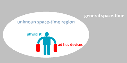
Figure 1: Epistemic relativity wants to provide the physicist with the baggage and protocols necessary to make gravimetry in any unknown region of arbitrary space-times.

This is the first and unavoidable step to develop experimental relativity as the natural scientific approach to the physical world.

The basis of relativistic gravimetry are Einstein equations, and these equations need a precise mathematical model of the space-time. The adequacy of this mathematical model and the physical space-time that it describes implies a one-to-one correspondence between the points of the model and the physical events they describe. And because in the mathematical model points are precisely identified (by their coordinates), we need to know how to locate the events in the physical space-time.

What else do we need in epistemic relativity? In fact, what we need is to transform the space-time region of physical interest in a (finite) laboratory.

But, what is a laboratory in relativity? In fact, a reflection on this matter shows that any laboratory, regardless of the specificity of its measurement devices, has to provide us with:

• a precise physical location of the significant parts of the system, and

• a precise physical description of its intrinsic properties.

The devices able to carry out these two tasks are called relativistic positioning systems and relativistic stereometric systems respectively. Thus:

A finite laboratory in relativity is a space-time region endowed with

$\bullet$ a relativistic positioning system and

$\bullet$ a relativistic stereometric system.

The first task of epistemic relativity is to transform the finite regions of interest of the space-time in laboratories or, equivalently, to construct these two relativistic systems.

These two relativistic systems are sufficient to describe any experiment in their region of space-time. Remember that, as already mentioned, we refer to physical systems as relativistic objects, i.e. as worldlines or worldtubes so that they naturally contain the changes of state that the Newtonian physical systems at every instant may suffer during an experiment (they already are the histories or evolutions of Newtonian systems). With the same point of view, the physical properties of relativistic objects cannot but be the history of the physical properties of the Newtonian objects at every instant of its constituent events. It is thus clear that the two above functions of locating and detecting are effectively able to describe any physical experiment in the space-time domain in question.

3 Relativistic positioning systems

3.1 What is to locate

In general, to locate an object is to identify the place it takes up. To locate with accuracy objects of any size (avoiding vagueness such as “near of”, “inside of”, etc.), we need to assign a proper name to every event of the space in question. A locating system is a system of assignation of proper names to the events of a space.

In particular, because the space-time is a continuum, the assignation of a proper name to every one of its events has to be done with numbers. And because it is a four-dimensional continuum, every proper name has to be done with four numbers. So that, specifically, in (a region of) the space-time, a locating system is a system of assignation of four numbers to every one of its events.

In physics, the devices for assigning four numbers to every event may be constructed with different materials and be based in different physical properties, so that their specific construction and protocols of use give rise to different locating systems.

The set of tetrads of numbers generated in a region by a locating system constitutes (a physical realization of) a coordinate system. On the other hand, in topological manifolds, a coordinate system in a region $\cal{R}$ may be extracted from a local chart $(\cal{R},\varphi)$ by means of the coordinate functions associated to $\varphi$, where $\varphi$ is a homeomorphism from $\cal{R}$ to the associated linear space. We see that, mathematically, locating systems are represented by homeomorphisms $\varphi$. Thus, a locating system in a finite region $\cal{R}$ of the space-time may be seen as the physical construction of a local chart or, conversely, a local chart may be seen as a mathematical idealization of a locating system.

3.2 Properties of locating systems

According to the characteristics of the assignation system of coordinates, a locating system may be active if its assignation system only operates for events that emit signals of presence, or passive if it operates for all events of the region irrespective of their emission state; and it may be immediate if the values of the coordinates of every event are obtained without delay, or retarded otherwise. Also, according to its use, a locating system is said real if its assignation system starts one for all in all the region, and it is said virtual if it is used case by case to obtain only the specific coordinates of particular events.

Another classification takes into account the function allocated to the locating system. Two locating systems are of particular importance for us: reference systems, which allow one observer to know the coordinates of the events of the region and positioning systems, which allow every event of the region to know its proper coordinates.

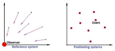
Figure 2: A reference system allows one observer to know the coordinates of the events of the region. A positioning system allows every event of the region to know its proper coordinates.

It is then evident that real locating systems may be immediate and passive, meanwhile virtual locating systems are necessarily active and retarded. And, taking into account that in relativity information propagates at a finite velocity, it results that all reference systems are retarded.

We can conclude that, when it is possible to construct them, real positioning systems are the locating systems that offer the best physical performances.

3.3 Relativistic positioning systems

We have just seen that, among all locating systems, the real positioning systems offer the performances of being passive and immediate. These performances are still insufficient for us because the main objective of epistemic relativity is to make relativistic gravimetry in an unknown space-time environment.

Because the space-time environment is unknown, the locating system has also to be generic, that is to say, able to be constructed in regions of any space-time. And because the main objective is to make relativistic gravimetry, it has also to be (gravitationally) free, i.e. able to be constructed without the previous knowledge of the space-time metric.

Relativistic positioning systems are the real, generic and free positioning systems of the space-time.

The construction of relativistic positioning systems is unexpectedly simple. A clock may be seen as a continuous generator of numbers, namely the time that it displays at every instant. Broadcasting this time by means of an electromagnetic signal, every event receiving the signal will know this number at the instant of reception. And because the proper name of every event of the space-time consists of four numbers (its coordinates), four clocks arbitrarily distributed will provide every event reached by the four signals with such numbers. It is thus easy to see that: Four clocks broadcasting their times constitute a relativistic positioning system (see [3]).

The coordinates generated by relativistic positioning systems are called emission coordinates [4].

Note: I have chosen to introduce the well-known notion of coordinate system in this unusual form because the traditional presentations induce to give too importance to ingredients that are in fact dispensable or of secondary interest, but wrongly make many people to feel them necessary to understand physically a coordinate system. Thus, ingredients like origin, coordinate lines or synchronization of a coordinate system are respectively irrelevant, of secondary interest or inexistent for relativistic positioning systems.

It is worthwhile to remark that relativistic positioning systems are a particular class of positioning systems but that, although similar in some aspects to positioning systems like GNSSs (global navigation satellite systems), differ clearly from them, whatever be the relativistic formalism with which these last ones are analyzed. These GNSSs are technical objects, wonder technical objects, with a lot of technical, social and even scientific applications. But they are not scientific objects. The reason is that they have been thought, calculated and constructed using consciously a defective theory, the Newtonian one, to construct a Newtonian space in the region between the Earth surface and the constellation of satellites, in which the International Atomic Time on the Earth surface is imposed on all the region as a Newtonian absolute time. The “relativistic effects”” are not used to improve the approximate Newtonian calculations and to obtain more precise values of the physical times involved, but to deform the values of these physical times so as to mimic an unphysical Newtonian time everywhere (the calculated “relativistic effects” are subtracted to the physical values, not added to the Newtonian calculations of them!).

The above comment is not at all a criticism of GNSSs: as technical objects, they have to be useful to us and give us what we ask them to give. For relational (technical, social) convenience, it is the case, in particular, of a universal time for all of us, be we on the Earth surface or at 15.000 km height, at rest or at whatever velocity. But, I think that it would be better to have, first of all, a scientific object, an R-GNSS (Relativistic GNSS) able to give us our proper physical time, the value of the gravitational field or proper local distances, whatever our position and velocity with respect to the Earth surface. The reason is that starting from such a scientific object, a simple software would be able also to mimic GNSSs with their absolute time everywhere. The (theoretical) question is not so much to improve GNSSs, but instead to construct cutting-edge scientific R-GNSSs.

There are no specific coordinates associated to GNSSs. Nevertheless, emission coordinates are an important tool in the study of relativistic positioning systems and in particular in R-GNSS. Among others, they suggest new questions, provide new results and allow the constellation of satellites of an R-GNSS to generate autonomous positioning systems for the Earth.

3.4 Auto-locating systems

As an intermediate step, auto-locating systems are those relativistic positioning systems whose clocks are endowed with a transponder broadcasting the times they receive from the other clocks of the system (see [3],[5] and references therein). So, every event $P$ of the region receives the sixteen times $\tau^{A}$ and $\tau^{AB}$ $A,B=1,...,4,A\neq B$. The four $(\tau^{A})$ are the emission coordinates of $P$, meanwhile every one of the four sets $A$ of four times $(\tau^{A},\tau^{AB})$ are the emission coordinates of the clocks $A$ of the system (see Fig. 3).

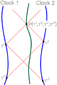
Figure 3: An auto-locating system allows any user to know its proper trajectory in emission coordinates, but also the trajectories of the clocks of the system (here a two-dimensional scheme).

Thus, any user that records these data is able to know its trajectory as well as the trajectories of the clocks in the grid of emission coordinates.

An echo-interval for the clock $A$ due to the clock $B$ is the segment of world line of $A$ from the instant of emission of a broadcast signal by $A$ to the instant that it receives that signal echoed by $B$. In two dimensions, it is already proved a very interesting theorem for auto-locating systems (see [5]):

Theorem 3.4-1 In a flat two-dimensional space-time, consider a user of an auto-locating system that knows its trajectory and those of the two clocks in the grid. If it also knows the acceleration of one of the clocks during one echo-interval, then it knows its acceleration and those of the two clocks along all their known trajectories.

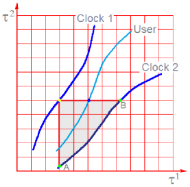
Figure 4: In absence of a gravitational field, a user of an auto-locating system is able to know its trajectory and that of the clocks in the grid of emission coordinates. If it also knows the acceleration of one of the clocks during one echo-interval AB, then it knows its acceleration and those of the two clocks along all their trajectories.

This theorem is very interesting because of the following fact: the algorithm that proves it in absence of a gravitational field may be as well applied in presence of it. Of course, in this case, it will provide a wrong acceleration along all the three trajectories excepting on the starting echo-interval of the clocks. But the importance of this fact is that the difference between these wrong accelerations (calculated as if the gravitational field were absent) and the true accelerations (measured by accelerometers along the world-lines of clocks and user in the gravitational field), is all the dynamical effect that the gravitational field produces on the auto-locating system and the user.

Thus, it is a complete, although relative (to the choice of echo-interval), gravimetric measure. Unfortunately, this fundamental theorem 3.4-1 is only know in two-dimensional space-times. It is of crucial importance for the theory of relativistic positioning systems and for all its near-future applications (Earth surface, RNGSS, Deep Space Navigation) to have its four-dimensional generalization. But this problem remains open. As in the two-dimensional case, the starting point is

• the explicit knowledge of the coordinate transformation between the emission coordinates of four arbitrarily accelerated clocks and inertial coordinates, and

• the explicit knowledge of the metric in emission coordinates.

Fortunately, the solution to these problems is already known. If the world-lines $\gamma_{A}(\tau^{A})$, $A=1,...,4,$ of four emitters with respect to inertial coordinates are known, we can evaluate the quantities

$$e_{a}\equiv\gamma_{a}-\gamma_{4}\quad,\quad\Omega_{a}\equiv\frac{1}{2}(e_{a})^{2}\quad,\quad\chi\equiv*(e_{1}\wedge e_{2}\wedge e_{3})$$

$$H\equiv*(\Omega_{1}\,e_{2}\wedge e_{3}+\Omega_{2}\,e_{3}\wedge e_{1}+\Omega_{3}\,e_{1}\wedge e_{2})\quad,\quad y_{*}\equiv\frac{1}{\xi.\chi}\,i(\xi)H$$

where $\xi$ is an arbitrary transversal vector, $\xi.\chi\neq 0$, and $a=1,2,3$. Then, the answer to the first item is (see [2] and [6]):

Theorem 3.4-2 Suppose known the world-lines $x=\gamma_{A}(\tau^{A})$ of the four emitters of a positioning system with respect to an inertial coordinate system $\{x\}$, and let $\{\tau^{A}\}$ be their emission coordinates. In term of the quantities $\chi$ and $y_{*}$ evaluated from the $\gamma_{A}(\tau^{A})$’s, the coordinate transformation $x=\kappa(\tau^{A})$ between emission and inertial coordinates is given by:

$$x\equiv\kappa(\tau^{R})=\gamma_{4}+y_{*}+\frac{y_{*}^{2}\,\chi}{(y_{*}\,.\,\chi)+\hat{\varepsilon}\sqrt{(y_{*}\,.\,\chi)^{2}-y_{*}^{2}\,\chi^{2}}}$$

where $\hat{\varepsilon}$ is the orientation of the position system with respect to the user.

And the answer to the second item is:

Theorem 3.4-3 In terms of the above transformation $x=\kappa(\tau^{R})$ and the world-lines $x=\gamma_{A}(\tau^{A})$, the contravariant components of the metric, $g^{AB}(\tau^{R})$, in the emission coordinates $\{\tau^{R}\}$ are given by:

$$g^{AB}(\tau^{R})=\frac{\Omega_{AB}}{\mu_{A}\,\mu_{B}}\quad,$$

where

$$\Omega_{AB}\equiv\frac{1}{2}(\gamma_{A}-\gamma_{B})^{2}\quad,\quad\mu_{A}\equiv(\kappa-\gamma_{A})\,.\,\dot{\gamma}_{A}\quad.$$

3.5 Autonomous positioning systems

Auto-locating systems contain all what a coordinate system needs in order to be drawn in a space in which a field of light-cones is given. But if the light-cones are specifically related to a geometry (here the gravitational field represented by a metric), and we want to identify individually the coordinate system making in it gravimetry (measure of the metric), we need additional information. This information has to be also broadcast by the clocks and consists of:

• dynamical data of the satellites (acceleration, gradiometry),

• observational data from them (e.g. particular masses, directions of reference quasars or pulsars, etc.), and

• gravitational knowledge of the coordinate region (theoretical, experimental or mixed).

This information constitutes the autonomous data. Autonomous positioning systems are auto-locating systems that broadcast autonomous data.

Autonomous positioning systems are, generically, the best locating systems we are able to construct. Their notion was already proposed in the first paper on positioning systems (see [3])

4 Relativistic stereometric systems

4.1 The notion

We already know that, to transform a finite region of the space-time in a laboratory, we need to endow it with, on one hand, a relativistic positioning system, to locate in the best form the significant parts of the physical system in question, and on the other hand, a relativistic stereometric system, to obtain their intrinsic physical properties.

Similarly to a relativistic positioning system, that consists essentially of four clocks broadcasting their times, a relativistic stereometric system consists of a system of four observers receiving the signals broadcast from a physical system.

In relativity, the word ‘observer’ is used in different contexts with different meanings. Here an observer means an eye able to record and to analyze the input, and an eye is a small (physically local, mathematically differential) object, determined by its space-time worldline, able to project its past light-cone on its celestial sphere.

Figure 5: An observer, determined by its unit velocity, projects its past light-cone on its celestial sphere.

There exist interesting papers on relativistic vision but they are very different in strategy, starting hypothesis and definition of ‘eye’, and their number is very small. It would be worthwhile to analyze and classify them, and especially to select those related to hypergon eyes.

But almost none of them consider the invariants of the observed figures. The study of these invariants is important for positioning as well as for stereometry. For example, any set of four events in the space-time (four stars in the sky or four material points of a system), that are seen on a circle of the celestial sphere of an observer, will be seen also on a circle, by any other observer at the same event, whatever be their relative velocity at the event. In addition, the relative velocity of such two observers may be obtained by comparison of the relative positions on the circle of the four points as seen by them.

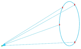
Figure 6: Four events that are seen in a circle on the celestial sphere of an observer are also seen in a circle on the celestial sphere of any other observer at the same event, whatever its relative velocity.

From the point of view of the space-time geometry, relativistic stereometric systems are the causal duals of relativistic positioning systems: the four observers (resp. four clocks) of the relativistic stereometric system (resp. relativistic positioning system) receive (resp. broadcast) the signals emitted by the event to be analyzed (resp. the signals received by the event to be located). As a consequence, every geometric result on one of these systems generates another geometric result for the other system, by a simple change of time orientation.

Figure 7: Relativistic stereometric systems are the causal duals of relativistic positioning systems.

Relativistic stereometric systems are conceived to obtain the intrinsic properties of physical systems but, in their basic structure, they are also locating systems. As locating systems, the coordinates of every event are the (four) times of reception by the (four) observers of the signal emitted by the physical system at this event. According to the properties considered in subsection 3.2, relativistic stereometric systems are active, retarded and virtual locating systems, in contrast with the passive, immediate and real properties of relativistic positioning systems. As we have seen in subsection 3.2, the active, retarded and virtual properties of relativistic stereometric systems are not the best as locating systems but, nevertheless, they are well adapted to the principal function of relativistic stereometric systems, because the intrinsic properties of a physical system cannot be obtained but by active, retarded and virtual ways. Thus, relativistic stereometric systems not only describe the intrinsic properties of events but also locate them.

4.2 First results in relativistic stereometry

Every observer of a relativistic stereometric system receives a (relativistic) perspective of the properties broadcast by the events. These four observer-dependent perspectives have to be combined in order to obtain the observer-invariant (proper or intrinsic) properties that generate them.

To show how to proceed, we shall present here the simplest case of relativistic stereometry, that of a material point broadcasting a signal in a flat two-dimensional space-time. In spite of its simplicity: (i) it leads to a simple but interesting extension of the unidirectional Doppler formula and (ii) it shows the difference between an ontic law and an epistemic one.

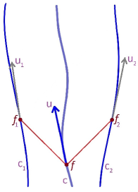
Figure 8: A two-dimensional relativistic stereometric system measuring the proper frequency $f$ of a material point.

Thus, let $C$, $C_{1}$ and $C_{2}$ be respectively the worldlines of a material point and of the two observers of the relativistic stereometric system in Minkowski space $M_{2}$. Suppose that at a particular instant $C$ broadcasts a signal of proper frequency $f$ that is received by $C_{1}$ and $C_{2}$ at the Doppler frequencies $f_{1}$ and $f_{2}$ respectively. Let $v_{1}$ and $v_{2}$ be the scalar relative velocities of $C$ with respect to $C_{1}$ and $C_{2}$ evaluated by them at the instants of reception of the frequencies $f_{1}$ and $f_{2}$ respectively. As it is well known, $f_{1}$ and $f_{2}$ are related to $f$ by the Doppler expressions:

$$f_{1}=f\sqrt{\frac{1-v_{1}}{1+v_{1}}}\quad,\quad f_{2}=f\sqrt{\frac{1-v_{2}}{1+v_{2}}}\quad.$$ (1)

Denoting by $v_{12}$ the relative scalar velocity of $C_{1}$ and $C_{2}$ at the instants of reception of the Doppler frequencies, one can prove:

Theorem 4.2-1.- In terms of the relative scalar velocity $v_{12}$ of the observers $C_{1}$ and $C_{2}$ of a relativistic stereometric system at the instant of reception of the Doppler frequencies $f_{1}$ and $f_{2}$ from a material point $C$, the proper frequency $f$ of the material point at the instant of emission is given by:

$$f^{2}=f_{1}f_{2}\sqrt{\frac{1+v_{12}}{1-v_{12}}}\quad.$$ (2)

Of course, if the material point is dragged by one of the observers of the system, say $f=f_{2}$, expression (2) coincides with the first of (1).

The Doppler frequencies also allow to know the relative velocities of the material point $C$ at the instant of emission of the signal with respect to the observers $C_{1}$ and $C_{2}$ at the instants of its reception. By elimination of $f$ from every one of the expressions (1) and (2), one has:

Theorem 4.2-2.- The relative velocities $v_{1}$ and $v_{2}$ of the material point $C$ at the instant of emission of the signal with respect to the observers $C_{1}$ and $C_{2}$ at the instants of its reception are given by:

$$v_{1}=\frac{f_{2}\sqrt{1+v_{12}}-f_{1}\sqrt{1-v_{12}}}{f_{2}\sqrt{1+v_{12}}+f_{1}\sqrt{1-v_{12}}}\quad,$$ (3)

$$v_{2}=\frac{f_{1}\sqrt{1+v_{12}}-f_{2}\sqrt{1-v_{12}}}{f_{1}\sqrt{1+v_{12}}+f_{2}\sqrt{1-v_{12}}}\quad.$$ (4)

The above results depend on the Doppler frequencies $f_{1}$ and $f_{2}$ but also on the quantity $v_{12}$, the scalar velocity of one of the observers of the relativistic stereometric system with respect to the other at the instants at which they receive the Doppler frequencies. This quantity cannot be measured directly, but has to be calculated in terms of other physical quantities. This reason is sufficient to show that the above two theorems, in their present form, do not constitute results of epistemic relativity. In fact, these two theorems do not fulfill any of the three conditions of subsection 2.1 characterizing epistemic relativity. For that, we must specify (i) what physicist we have chosen to make the experiment, (ii) when and where it will know the quantities needed to solve the problem and (iii) how can it know or measure these quantities. In the present case, we make the following choices:

• the physicist is one of the observers of the relativistic stereometric system, say $C_{2}$, as shown in Fig. 9,

• it will be informed of the pertinent quantities at the instant $\tau_{12}$ of reception of the information coming from the observer $C_{1}$,

• at that instant $\tau_{12}$, it already knows the quantity $f_{2}$ measured and recorded by itself, it is being informed of the quantity $f_{1}$, and then may know the quantity $v_{12}$ by computation.

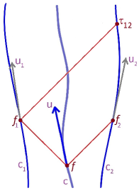
Figure 9: The observer $C_{2}$ has been chosen as the ‘physicist’. From the instant $\tau_{12}$ on, it may know all the quantities of the problem.

At the instant of reception of the signal $f_{1}$, the observer $C_{1}$, in addition to send its measure, must send also its reflection or its proper frequency so as to allow $C_{2}$ to know its relative velocity at its instant $\tau_{12}$. On the other hand, $C_{2}$ is supposed to know its proper acceleration, so that it is able to know its relative velocity between its instant of reception of the signal $f_{2}$ and the instant $\tau_{12}$. The knowledge of these two velocities, allow it to calculate the velocity $v_{12}$ of the theorems. For simplicity, suppose here that $C_{2}$ is geodesic. Then, the relative frequency between the proper time of $C_{1}$ at the instant of reception of the frequency $f_{1}$ and the proper time of $C_{2}$ at any instant is constant. Denoting it by $\nu_{12}$ and inverting the Doppler formula we have:

$$v_{12}=\frac{1-\nu_{12}^{2}}{1+\nu_{12}^{2}}\;.$$ (5)

Now if, for short, we call an epistemic theorem an ‘epistem’, the above two theorems in this geodesic case become respectively:

Epistem 1.- In terms of the frequencies $f_{1}$ and $f_{2}$ received by a relativistic stereometric system $\{C_{1},C_{2}\}$ from a material point $C$ and of the relative frequency $\nu_{12}$ of the proper time of the observer $C_{1}$ with respect to the geodesic observer $C_{2}$, the proper frequency $f$ of the material point $C$ is given by:

$$f^{2}=\frac{f_{1}f_{2}}{\nu_{12}}\;.$$ (6)

Epistem 2.- In terms of the frequencies $f_{1}$ and $f_{2}$ received by a relativistic stereometric system $\{C_{1},C_{2}\}$ from a material point emitter $C$ and of the relative frequency $\nu_{12}$ of the proper time of the observer $C_{1}$ with respect to the geodesic observer $C_{2}$, the relative velocities $v_{1}$ and $v_{2}$ of the material point $C$ with respect to the observers $C_{1}$ and $C_{2}$ at the instants of reception of the signals $f_{1}$ and $f_{2}$ are given by:

$$v_{1}=\frac{f_{2}-f_{1}\nu_{12}}{f_{2}+f_{1}\nu_{12}}\quad,\quad v_{2}=\frac{f_{1}-f_{2}\nu_{12}}{f_{1}+f_{2}\nu_{12}}\,.$$ (7)

These results are very simple, but show roughly the way of working with stereometric systems in epistemic relativity. Of course, the problem of determining the proper distances to its neighboring elements of a material point cannot be considered in a two-dimensional space-time, because there the celestial sphere of an observer reduces to two opposite points. It is evident that this work has to be extended and generalized in three and four dimensions. It remains an open problem.

5 Intrinsic characterization of gravitational fields

In epistemic relativity, events are located in emission coordinates generated by relativistic positioning systems.

A complete set of gravimetric measurements (whatever be the methods) will lead to the experimental values of the components of the metric in emission coordinates.

It rests to identify this metric or, equivalently, its sources. For example, suppose we suspect that it corresponds either to a Kerr or to a Schwarzschild gravitational field, but that it can be neither one nor the other. How can we discern between these three possibilities?

The most part of the known gravitational fields (exact or approximate solutions to Einstein equations), and in particular Kerr and Schwarzschild, are known in very particular coordinate systems which have no simple relation with emission coordinates.

For example, for the Schwarzschild case, the direct procedure would be

• to calculate in Schwarzschild coordinates the equations of the field of light-cones,

• to model in these coordinates the world-lines of the clocks of the positioning system, parameterized with their proper time,

• to select with both results the four families of light-cones emitted by the clocks or, in other words, to obtain the transformation from emission coordinates to the Schwarzschild ones,

• to solve for the inverse transformation,

• to transform the Schwarzschild metric components in emission metric components,

• to compare them with the experimental values obtained in these emission coordinates.

Every one of these items presents non-negligible difficulties and can introduce specific uncertainties. It results in a hard and long procedure.

For this reason, to compare the experimental value of the gravitational field obtained in emission coordinates with a given solution of Einstein equations, it may be better to characterize intrinsically the solution and to check if the experimental data verify this characterization.

By intrinsic characterization of a metric we understand here a set of necessary and sufficient local conditions on some of the concomitants of the metric that characterize it, its sources and their position, regardless of the coordinate system.

The idea is that an observer, from the sole measure of the gravitational field and its variations in a local region, is able to know the masses that produce it as well as its positions with respect to it.

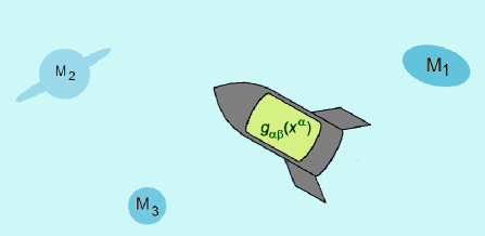
Figure 10: An observer that measures the gravitational field in a local space is able to know the masses that produce them as well as their positions.

The intrinsic characterization of individual metrics is, apart from some trivial cases, a relatively recent problem. I would like to draw attention on the pertinence not only of its development for all exact solutions of Einstein equations of physical interest but also of its extension to the usual approximate solutions in experimental applications. By the reason above indicated, I believe this characterization to be the simplest and shortest way to identify gravitational fields in epistemic relativity.

The idea to characterize individual metrics intrinsically originates some years ago as part of a general project of IDEAL solution of problems, somehow similar in spirit to that of classic Greek mathematicians but of vivid actuality for the problems we were concerned, where the acronym stands for

• Intrinsic (depending only on the concepts mentioned in the statement of the problem),

• Deductive (not involving inductive or inferential methods or arguments),

• Explicit (expressing the elements of the solution not implicitly) and

• Algorithmic (giving the solution as a flow chart with a finite number of steps).

The first solution intentionally obtained under the IDEAL spirit was that of the point particle in Newtonian gravity ([7]). I cite it here because the solution to its relativistic analog, the Schwarzschild gravitational field, in contrast with an extended opinion but like many other generic problems, admits simpler expressions than that of Newtonian physics.

The intrinsic characterization of the Schwarzschild gravitational field is due to J. Ferrando and J.A. Sáez ([8]). Denoting by $Riem$ the Riemann tensor, by $tr$ and $i(.)$ the trace operator and the interior product respectively, and by $\wedge$ the exterior product (considering the metric $g$ as a double 1-form), they introduce the two scalars:

$$\sigma\equiv\left(\frac{1}{12}tr^{2}Riem^{3}\right)^{\frac{1}{3}}\quad,\quad\alpha\equiv\frac{1}{9\,\sigma^{2}}\,g(d\sigma,d\sigma)+2\sigma\quad,$$ (8)

allowing to construct the two tensors:

$$S\equiv-\frac{1}{3\,\sigma}\left(Riem+\frac{1}{2}\sigma g\wedge g\right)\quad,\quad Q\equiv i^{2}(d\sigma)S\quad.$$ (9)

and, with the help of an arbitrary direction $x$, generate a third, direction-dependent scalar $\theta$:

$$\theta(x)\equiv 2Q(x,x)+trQ\quad.$$ (10)

These quantities may be evaluated for any gravitational field, and involve the gradient of a function of $Riem$, a third variation of the metric.

Their first result is:

Theorem 5-1.- A vacuum metric $g$, $Ric(g)=0$, is the Schwarzschild metric if, and only if, the three scalars $\sigma$, $\alpha$ and $\theta$ are strictly positive,

$$\sigma>0\quad,\quad\alpha>0\quad,\quad\theta(x)>0\quad,$$ (11)

and the two following tensors vanish:

$$i^{2}(d\sigma)\ast\!\!Riem=0\quad,\quad S^{2}+S=0\quad,$$ (12)

where $\ast$ is the Hodge duality operator.

In the circumstances suggested by Fig. 10 this result assures the experimental physicist, whatever the coordinates used, that it is immersed in the field of a spherically symmetric mass. But what mass and where? The answer is also given in [8]:

Theorem 5-2.- The mass $m$ and the radial coordinate $r$ of a Schwarz-schild metric are given by:

$$m=\sigma\alpha^{-\frac{3}{2}}\quad,\quad r=\alpha^{-\frac{1}{2}}\quad.$$ (13)

In fact, any other intrinsic characteristic of Schwarzschild metric may be obtained in an IDEAL way. For example, differentiating the second of relations (13) one obtains the intrinsic expression in terms of the invariant $\alpha$ of the radial codirection $-dr$ of the mass, allowing the physicist to know its direction, distance and value. Also, on the event horizon $r=2m$ one would find $\alpha$ $=2\sigma$ and, as (8) shows, also $g(d\sigma,d\sigma)$ would vanish. Furthermore, as proven also in [8], the time-like direction of static evolution of the gravitational field, i.e. its integrable Killing vector field $\xi$, is given by:

$$\xi=-\sigma^{-\frac{4}{3}}\frac{Q(x)}{\sqrt{Q(x,x)}}\quad.$$ (14)

These results already allow us to appreciate the interest of local intrinsic characterizations of gravitational fields. But they are far from being only the characterization of the simplest gravitational field. The scalars $\sigma$, $\alpha$ and $\theta$, in (8) and (10), and the tensors $S$ and $Q$, in (9), may be evaluated in any gravitational field and their comparison with relations (11) and (12) will give us an information that we would study in detail, in particular if the gravitational field in question may be well described as a Schwarzschild perturbation.

At present, the intrinsic characterization of some other classes of vacuum exact solutions of Einstein equations are known, in particular, Kerr metric (see [9] and references therein). We need to extend these results and, especially, develop these techniques for approximate solutions.

The above expressions, simple for a theoretical physicist, may seem complicated for an experimental one. They need to be broken down in measurable terms so as to conceive the devices and procedures to measure them. But there is no doubt that the questions that local intrinsic characterizations of metrics allow to decipher, deserve a deeper study.

6 Finite-differential geometry

As it is well known, the mathematical substratum of general relativity is Lorentzian differential geometry. It thus follows that differential geometric methods are unavoidable in relativity. But there exist many situations in which these differential methods appear to be manifestly insufficient.

Among these situations, there are specific epistemic ones, involving the physical description in real time and by arbitrary observers of general variable gravitational fields, but also situations much more near of our usual ones in Earth’s relativity.

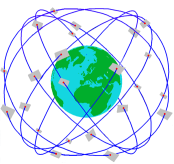
Figure 11: A constellation $\cal C$ of satellized clocks around a mass $M$, every tetrad of them working as an auto-locating system, recording the data set $\Lambda$ of all the signals emitted and received between them.

Thus, in a vacuum space-time, consider a mass $M$, not necessarily spherical, and a constellation $\cal C$ of satellized clocks around $M$ and such that every tetrad of them works as an auto-locating system. Let $\Lambda$ be the data set of all the signals that every clock emits and receives both, as an element of all the auto-locating systems at which it belongs and as a user of the auto-locating systems constituted by all the other clocks.

Suppose we know the mass $M$ and the world-lines of the constellation $\cal C$. We can model the system as follows. Start from the space-time metric around $M$, integrate the geodesic equations and specify them for every one of the clocks so as to model the whole constellation $\cal C$. Then, integrate the equations of the light-cones, either starting from the general solution of the null geodesic equations or integrating the geodesic distance function and considering its vanishing, so as to model any signal able to be emitted or received by any of the clocks of the constellation $\cal C$. With these two modeled ingredients, we are able to predict any of the data of the set $\Lambda$ received or emitted by any of the clocks in terms respectively of the data emitted or received by all the other clocks.

The physical interest of such a mathematical model is not, however, very intense. On the contrary, the following scenario could be the prelude to a fine gravimetry of the Earth … if we were able to develop the adequate mathematical instrument.

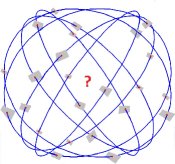
Figure 12: When we know the constellation of satellites $\cal C$ and the data set $\Lambda$, how to obtain the mass $M$?

Suppose now that we know the constellation $\cal C$ and the data set $\Lambda$, and that we want to obtain the mass $M$. At present, the only way we know to tackle the problem is the above model, but for this scenario, it is heavy and unadapted to the starting point, the data set $\Lambda$. Indeed, $\Lambda$ consists of time-like distances (geodesic time intervals between any two events on the world-line of every clock) and null distances (light links between every pair of clocks), that is to say, of values of the distance function between pairs of events causally separated. For this reason, any direct method to model this scenario would start with the obtainment, from the data set $\Lambda$, of the metric distance function by means of a suitable interpolation method. This is part of the adequate mathematical instrument that we would be able to develop for obtaining the mass $M$. But it is still insufficient.

The objective of finite-differential geometry is to study finite and interchangeable versions of the ingredients of differential geometry (metric, connection, curvature). Because for general relativity the basic ingredient is the metric $g$, and that its finite version, the distance function, already poses problems, we shall consider it here.

It is well known that the finite version of the metric $g$ is the distance function $D(x,y)$, or its half-square $\Omega(x,y)$, the Synge’s world-function,

$$\Omega(x,y)\equiv\frac{1}{2}D(x,y)^{2}\quad,$$ (15)

given by

$$\Omega(x,y)=\frac{1}{2}\int^{1}_{0}g\left(\frac{d\gamma}{d\lambda},\frac{d\gamma}{d\lambda}\right)d\lambda\quad,$$ (16)

and verifying its fundamental equations:

$$g^{\alpha\beta}\partial_{\alpha}\Omega\partial_{\beta}\Omega=2\Omega\quad,\quad g^{ab}\partial_{a}\Omega\partial_{b}\Omega=2\Omega\quad,$$ (17)

where Greek indices correspond to coordinates at the point $x$ and Latin ones to the point $y$.

Mathematically, distance spaces, i.e. manifolds endowed with a distance function, are well known, but their link with differential geometry have not been sufficiently explored.

An important obstruction for the interchangeability between the differential and the finite concept is that the most part of distance functions are not geodesic distance functions of any metric. It is known that, when a distance function $D(x,y)$ is the geodesic distance function of a metric, this metric may be obtained as minus the limit $y\rightarrow x$ of the mixed first derivatives of the half square (Synge’s world function) of the distance function. If this limit is applied to an arbitrary distance function, it may give rise to a zero, degenerate or regular metric. But, even when this metric is regular, the distance function $D(x,y)$ will not be generically the geodesic distance function of it. Suppose, in our physical case, that the interpolated distance function from the data set $\Lambda$ is at least of differentiability class 2. We can obtain a metric from the above limiting process, but this metric will strongly depend on the interpolation method used, for which we have no control. For this and other applications, to discern if a distance function is a geodesic distance function of a metric, it would be convenient to have an IDEAL criterion involving solely the distance function, without any limiting process.

I solved this problem some years ago. Let us introduce the following quantities of the first and second derivatives of the distance function $D(x,y)$:

$$V_{\ell mn}^{\alpha}\equiv\epsilon^{\alpha\lambda\mu\nu}D_{\ell\lambda}D_{m\mu}D_{n\nu}\quad,\quad V^{a\alpha}\equiv\epsilon^{a\ell mn}\epsilon^{\alpha\lambda\mu\nu}D_{\ell}D_{\lambda}D_{m\mu}D_{n\nu}\quad,$$ (18)

as well as the quantity:

$$V^{\alpha}\equiv V_{\ell mn}^{\alpha}x^{\ell}y^{m}z^{n}\;,$$ (19)

where $x^{\ell}$, $y^{m}$, $z^{n}$ are arbitrary independent directions. Define the two scalars

$$\Phi\equiv D_{\lambda}V^{\lambda}\quad,\quad\Psi\equiv\epsilon^{r\ell mn}V_{\ell mn}^{\rho}D_{r}D_{\rho}\quad,$$ (20)

and form the two quantities:

$$D^{\alpha}\equiv\frac{V^{\alpha}}{\Phi}\quad,\quad D^{a\alpha}\equiv 3\frac{V^{a\alpha}}{\Psi}\;.$$ (21)

Then, we have:

Theorem 6-1.- (Structure theorem for geodesic distance functions.) The necessary and sufficient condition for a distance function $D(x,y)$ to be the geodesic distance function of a metric, is that its derivatives verify:

$$D^{\rho}D_{abc\rho}+D^{\rho}D^{m\sigma}\oint_{abc}(D_{am\rho}-D^{n}D_{mn\rho}D_{a})D_{bc\sigma}=0$$ (22)

where the subscripts denote partial derivatives and $D^{a}$ and $D^{a\alpha}$ are the quantities just defined.

In our physical case, these are the constraints to be imposed directly to any interpolated distance function on the data set $\Lambda$. Once these equations verified at the suitable degree of precision, one has to extract the metric from this distance function without any limiting process. I solved this problem together with the above one. The result is:

Theorem 6-2.- (Metric of a geodesic distance function.) In terms of the partial derivatives $D_{\alpha},$ $D_{a\alpha}$ and $D_{ab\alpha}$ of a geodesic distance function, the contravariant components $g^{\alpha\beta}$ of the metric at the point $x,$ are given by

$$g^{\alpha\beta}=D^{\alpha}D^{\beta}+D^{a\alpha}D^{b\beta}D_{ab\gamma}D^{\gamma}\quad,$$ (23)

where $D^{\alpha}$ and $D^{a\alpha}$ are the quantities above defined.

Coming back to our physical case, (23) would give us the metric in the region of the constellation. Then, the intrinsic characterization method of Section 5, once generalized to perturbations of Schwarzschild gravitational field, would give us the mass $M$ that satellizes the constellation $\cal C$ and generates the data set $\Lambda$.

Theorems 6-1 and 6-2 give to the distance function $D(x,y)$ the interchangeable character with its differential homolog, the metric $g(x)$, that our finite-differential geometry requires. But finite-differential geometry has to be developed in many other directions. Among them, perhaps the more urgent ones are the development of methods of interpolation and approximation of distance functions.

References

- [1] B. Coll, Relativistic positioning systems: perspectives and prospects. Acta Futura, 7 35-47, 2013.
- [2] B. Coll J. J. Ferrando and J. A. Morales-Lladosa. Positioning systems in Minkowski space-time: from emission to inertial coordinates. Class. Quantum Grav., 27:065013, 2010.
- [3] B. Coll. Elements for a theory of relativistic coordinate systems. Formal and physical aspects. Proceedings of the Spanish Relativity Meeting 2000 on Reference Frames and Gravitomagnetism (Valladolid, Spain), pages 53-65, World Scientic, Singapore, 2001.
- [4] B. Coll and J. M. Pozo. Relativistic positioning systems: the emission coordinates. Class. Quantum Grav., 23:7395, 2006.
- [5] B. Coll J. J. Ferrando and J. A. Morales-Lladosa. Positioning in a at two-dimensional space-time: the delay master equation. Phys. Rev. D, 82:084038, 2010.
- [6] B. Coll J. J. Ferrando and J. A. Morales-Lladosa. Positioning in Minkowski space-times: Bifurcation problem and observational data. Phys. Rev. D, 86:084036, 2012.
- [7] B. Coll and J. J. Ferrando. The Newtonian Point Particle. Proceedings Spanish Relativity Meeting 1997 (Palma de Mallorca, Spain), pages 184- 190, Pub. Univ. Illes Balears, 1997.
- [8] J. J. Ferrando and J. A. Sáez. An intrinsic characterization of the Schwarzschild metric. Class. Quantum Grav., 15:1323, 1998.
- [9] J. J. Ferrando and J. A. Sáez. An intrinsic characterization of the Kerr metric. Class. Quantum Grav., 26:075013, 2009.