On the frequency dependence of p-mode frequency shifts induced by magnetic activity in Kepler solar-like stars

The variations of the frequencies of the low-degree acoustic oscillations in the Sun induced by magnetic activity show a dependence with radial order. The frequency shifts are observed to increase towards higher-order modes to reach a maximum of about 0.8 $\mu$Hz over the 11-yr solar cycle. A comparable frequency dependence is also measured in two other main-sequence solar-like stars, the F-star HD 49933, and the young 1-Gyr-old solar analog KIC 10644253, although with different amplitudes of the shifts of about 2 $\mu$Hz and 0.5 $\mu$Hz respectively. Our objective here is to extend this analysis to stars with different masses, metallicities, and evolutionary stages. From an initial set of 87 Kepler solar-like oscillating stars with already known individual p-mode frequencies, we identify five stars showing frequency shifts that can be considered reliable using selection criteria based on Monte Carlo simulations and on the photospheric magnetic activity proxy $S_{\text{ph}}$. The frequency dependence of the frequency shifts of four of these stars could be measured for the $l=0$ and $l=1$ modes individually. Given the quality of the data, the results could indicate that a different physical source of perturbation than in the Sun is dominating in this sample of solar-like stars.

1 Introduction

The first detection of the signature in the acoustic (p) oscillation parameters of a magnetic activity cycle was observed with the Convection, Rotation, and planetary Transits (CoRoT; Baglin et al., 2006) space telescope in the F-type solar-like star HD 49933 (García et al., 2010). It demonstrated that asteroseismology can provide new and original constraints for the study of stellar magnetic activity and dynamo models under conditions different from those of the Sun. Since then, additional studies were performed using the long and continuous observations collected by the NASA Kepler telescope (Borucki et al., 2010). Changes in the characteristics of the p-mode frequencies as a consequence of their surface magnetism have been studied now in a handful of solar-like stars (Salabert et al., 2016; Régulo et al., 2016; Kiefer et al., 2017, Karoff et al. submitted; Santos et al., in preparation), suggesting that the frequency shifts decrease with stellar age and rotation period (Kiefer et al., 2017).

The frequency dependence of the p-mode frequency shifts can provide insights on the structural changes of the stellar interior with magnetic activity. In the case of the Sun, the frequency shifts are known to increase with frequency as first shown by Libbrecht & Woodard (1990) and Anguera Gubau et al. (1992) for the intermediate- and low-degree modes respectively. Such dependence is explained as a consequence of changes in the outer layers of the Sun just beneath the solar photosphere (e.g., Libbrecht & Woodard, 1990; Chaplin et al., 1998; Salabert et al., 2004). Moreover, similar frequency dependence of the shifts was also found in HD 49933 (Salabert et al., 2011) and in the G0-type KIC 10644253 (Salabert et al., 2016). This latter star is particularly interesting as this young solar analog (1 Gyr-old) has an amplitude of the frequency shifts comparable to the Sun (Salabert et al., 2016). Metcalfe et al. (2007) and Chaplin et al. (2007a) formulated two different predictions of the expected frequency shifts based on scaling relations with the strength of the Ca ii H and K emissions. For a given stellar age, the predicted shifts proposed by Metcalfe et al. (2007) get larger for hotter stars, while the ones by Chaplin et al. (2007a) show almost no variation with temperature. The results for the F-star HD 49933 corroborate the formulation from Metcalfe et al. (2007), while given the approximations considered and the observational uncertainties, the results for KIC 10644253 cannot favor any of the two predictions. Nonetheless, the analysis from Kiefer et al. (2017) of a sample composed of 24 solar-like stars would support the scaling relation proposed by Metcalfe et al. (2007).

The light-curve variability associated with the presence of spots rotating on the stellar surface provides another manner to study the global magnetic activity of stars. To cancel out the other sources of stellar variability at different timescales, such as the granulation or the oscillations, one needs to take into account the rotation period of the star when calculating such global photometric activity proxy, referred as the $S_{\mathrm{ph}}$ index (Mathur et al., 2014a). Several studies of the magnetic activity of main-sequence stars (Mathur et al., 2014b; García et al., 2014a; Ferreira Lopes et al., 2015; Salabert et al., 2016) observed with CoRoT and Kepler were performed based on the $S_{\mathrm{ph}}$. However, the $S_{\text{ph}}$ index is dependent on the inclination angle of the rotation axis of the star in respect to the line of sight, and thus represents a lower limit of stellar activity. This is of course supposing that starspots are formed over comparable latitunal bands as for the Sun. Nevertheless, the distribution of the spin orientation of field stars is observed to be consistent with an isotropic distribution (see e.g., Corsaro et al., 2017; Kuszlewicz, 2017), resulting in a most observed inclination angle close to 90^∘, hence perpendicular to the line of sight. On the other hand, in exo-planet systems the distribution could differ from isotropy (see e.g., Winn et al., 2006; Hirano et al., 2014). The observed isotropy for field stars implies that the $S_{\text{ph}}$ index thus measured represents the actual level of activity for most of the stars and not a lower limit. Furthermore, comparisons with several standard solar activity proxies sensitive to different layers of the solar photosphere and chromosphere show that both the long- and short-term magnetic variabilities are well monitored with the $S_{\text{ph}}$ proxy (Salabert et al., 2017).

In this work, we want to extend this analysis to a larger sample of solar-like stars with different fundamental parameters. The objective here is to make progress in the understanding of the physical mechanisms responsible of the perturbations inducing the variability of the p-mode oscillations with magnetic activity. We started with a sample of 87 solar-like pulsating stars observed by Kepler and for which the peak-fitting analysis of the individual modes can be found in the literature (Appourchaux et al., 2012; Lund et al., 2017). The reason for selecting this sample is threefold: (1) it allowed us to study stars from the three following categories depending to their seismic and spectroscopic properties: the simple stars, the F-type stars, and the mixed-mode stars (for more details, see Appourchaux et al., 2012); (2) the characterization of the individual modes of these stars is already available and their fundamental stellar properties determined (Mathur et al., 2012; Metcalfe et al., 2014; Creevey et al., 2017; Silva Aguirre et al., 2017); (3) these stars were observed in short cadence (SC; for more details, see Gilliland et al., 2010) for at least 1 year. The SC Kepler observations actually cover more than 3.5 years for most of these 87 stars.

The paper is organized as follows. In Section 2, we describe the Kepler observations used here. The methods applied to derive the frequency shifts of the acoustic oscillations and the contemporaneous photometric magnetic activity proxy $S_{\text{ph}}$ are described in Section 3. In Section 4, we define selection criteria based on Monte Carlo simulations to determine if the extracted variations of the frequency shifts are likely to be genuine signatures of magnetic variability or most likely due to noise. This is complemented by a selection criterion measuring the correlation between the frequency shifts and the $S_{\text{ph}}$ proxy. Based on these selection criteria, only few stars are found to show frequency shifts related to magnetic activity as presented in Section 5. A discussion on the frequency dependence of the frequency shifts is proposed in Section 6. Conclusions are presented in Section 7.

Table 1: List of the 87 solar-like oscillating stars observed by Kepler analyzed in this work. The full table will be available in the on-line version.

KIC	Years	Duty cycle	Category
		(%)
1435467	3.73	82.7	F-like
2837475	3.81	81.1	F-like
3424541	3.73	82.7	F-like
3427720	4.00	77.5	simple
3456181	2.54	51.3	F-like
3632418	3.73	82.7	simple
3656476	4.00	58.2	simple
3733735	3.81	81.1	F-like
3735871	3.89	79.4	F-like
4914923	4.00	71.2	simple
5184732	3.81	67.6	simple
5607242	3.89	79.4	mixed-modes
5773345	2.65	48.8	F-like
5950854	2.11	57.1	simple
5955122	4.00	77.5	mixed-modes
6106415	3.72	59.7	simple
6116048	3.81	81.1	simple
6225718	3.65	77.3	simple
6508366	4.00	77.5	F-like
6603624	4.00	77.5	simple
6679371	3.73	82.7	F-like
6933899	3.89	79.4	simple
…

2 Observations

Our initial sample consists in the 61 solar-like oscillating stars observed by Kepler analyzed in Appourchaux et al. (2012) complemented by 26 dwarfs from the LEGACY sample of 66 stars in Lund et al. (2017) and not included in Appourchaux et al. (2012). These 87 stars containing main-sequence and slightly more evolved stars are listed in Table LABEL:table:table_kic, where the total length of the observations and the associated duty cycles are given as well. This set of stars consists of Kepler targets which were observed for at least 12 months in SC ($\Delta t\simeq 58.9$ sec, Gilliland et al., 2010). The details of the observed and missing quarters can be found in Table 1 of Lund et al. (2017). These stars are categorized within three groups: (1) the simple stars with a clear mode identification; (2) the F-like stars for which the mode identification is ambiguous; and (3) the more evolved mixed-mode stars for which the acoustic modes do not follow the asymptotic relation.

In this work, we used both the SC to perform the asteroseismic analysis of the frequency shifts of the acoustic oscillations, and the long-cadence (LC, $\Delta t\simeq 29.4$ min, Jenkins et al., 2010) observations to study the temporal evolution of the photometric activity proxy $S_{\text{ph}}$ derived from the light-curve fluctuations. Both SC and LC observations were corrected for instrumental problems with the Kepler Asteroseismic Data Analysis and Calibration Software (KADACS, García et al., 2011). All the small gaps in the SC data were finally interpolated using an in-painting technique (García et al., 2014b; Pires et al., 2015).

3 Measurement of the magnetic activity variability

3.1 Extraction of the oscillation frequency shifts

3.1.1 Cross-correlation analysis (Method #1)

The cross-correlation method returns a global value of the frequency shift for all the visible modes in the analyzed frequency range of the power spectrum (Method #1). It was introduced by Pallé et al. (1989) to measure the variations of the solar oscillation frequencies of the $l=0,1$, and 2 acoustic modes during cycles 21 and 22 from one single ground-based instrument located in Tenerife. The method has since then been widely used to study the frequency shifts from helioseismic (see Chaplin et al., 2007b, and references therein) and asteroseismic (García et al., 2010; Régulo et al., 2016; Salabert et al., 2016; Kiefer et al., 2017) observations.

For each of the 87 stars in our sample, the Kepler SC time series were split into contiguous 90-day-long subseries, shifted by 30 days. The power spectrum of each 90-day subset was then cross correlated with a reference spectrum taken as the averaged spectrum of the independent spectra. The cross correlations were computed over frequency ranges, $\Delta\nu_{\text{range}}$, centered around the frequency of the maximum of the p-mode power excess, $\nu_{\text{max}}$, taken from Appourchaux et al. (2012) and Lund et al. (2017). As the large frequency separation between consecutive radial orders decreases as $\nu_{\text{max}}$ goes towards lower frequencies, three frequency ranges to compute the cross correlation were defined as follows: (1) if $\nu_{\text{max}}>1100\,\mu$Hz , $\Delta\nu_{\text{range}}=\pm\,400\,\mu$Hz around $\nu_{\text{max}}$; (2) if $800\,\mu$Hz $\leq\nu_{\text{max}}\leq 1100\,\mu$Hz, $\Delta\nu_{\text{range}}=\pm\,300\,\mu$Hz; and (3) if $\nu_{\text{max}}<800\,\mu$Hz , $\Delta\nu_{\text{range}}=\pm\,200\,\mu$Hz. Doing so, we ensure to select all the visible modes for each star, although for the cross-correlation method, the p modes with lower heights –located at each end of the frequency range– have very low weight and the obtained results are thus mostly sensitive to the higher modes around $\nu_{\text{max}}$.

To estimate the frequency shift $\delta\nu(t)$, the cross-correlation function was fitted with a Gaussian profile, whose centroid provides a measurement of the mean $l=0,1,$ and 2 mode frequency shift over the considered frequency range. The associated 1$\sigma$ uncertainties were obtained through Monte Carlo simulations as follows: the reference spectrum was shifted in frequency by the mean frequency shift obtained for each subseries; then 500 simulated power spectra were computed by multiplying the shifted reference spectrum by a random noise with a distribution following a $\chi^{2}$ with 2 degrees of freedom. For each sub spectrum, the standard deviation of all the shifts obtained from the 500 simulated spectra with respect to the corresponding reference spectrum was adopted as the 1$\sigma$ error bar of the fit. A detailed description of the method can be found in Régulo et al. (2016).

3.1.2 Individual mode peak-fitting analysis (Method #2)

As explained in Section 3.1.1, the cross-correlation method returns a global value of the frequency shift for all the visible $l=0,1$ and 2 modes in the power spectrum averaged over a given frequency range. The peak-fitting analysis provides the possibility to study separately the modes with different angular degrees and to have access to the frequency dependence of the frequency shifts (Method #2). It gives access as well to the other acoustic parameters, such as the mode heights and widths for instance.

For the peak-fitting analysis, 180-day-long subseries of the SC data were used with an overlap of 30 days. This length provides enough frequency resolution to retrieve the individual modes with accuracy. It offers also the possibility to extract the frequency shifts over independent subseries compared the cross-correlation analysis (Method #1). The power spectrum of each 180-day subseries was then obtained in order to extract estimates of the oscillation parameters. The individual frequencies of the angular degrees $l=0$, 1, and 2 provided by Appourchaux et al. (2012) and by Lund et al. (2017) were taken as initial guesses. The analysis was performed by fitting sequences of successive series of $l=0$, 1, and 2 modes using a maximum-likelihood estimator as in Salabert et al. (2011) for the CoRoT target HD 49933 and in Salabert et al. (2016) for the young solar-analog Kepler target KIC 10644253. The individual $l=0$, 1, and 2 modes were modeled using a Lorentzian profile for each of the angular degrees. Therefore, neither rotational splitting nor inclination angle were included in the fitting model. The height ratios between the $l=0$, 1, and 2 modes were fixed to 1, 1.5, and 0.5 respectively (Ballot et al., 2011), and only one linewidth was fitted per radial order $n$. The natural logarithms of the mode height, linewidth, and background noise were varied resulting in normal distributions. The formal uncertainties in each parameter were then derived from the inverse Hessian matrix. The mode frequencies thus extracted were checked to be consistent within 1$\sigma$ errors with Appourchaux et al. (2012) and Lund et al. (2017).

The mean temporal variations of the frequencies were defined as the differences between the frequencies observed at different dates and reference values of the corresponding modes. The set of reference frequencies was taken as the average over the entire observations. The frequency shifts thus obtained were then averaged over the same frequency ranges as the ones used for the cross-correlation analysis defined in Section 3.1.1. As the cross-correlation method returns mean frequency shifts unweighted over the analyzed frequency range, we decided to use unweighted averages of the frequency shifts extracted from the individual frequencies. We also note that we did not use the frequencies of the $l=2$ modes because of their lower signal-to-noise ratios.

Additionally, we analyzed the temporal variations of the power and damping of the p-mode oscillations. Indeed, these physical properties are known to be sensitive to magnetic activity as observed in the Sun (see e.g., Pallé et al., 1990; Elsworth et al., 1993; Chaplin et al., 2000; Howe et al., 2003; Salabert & Jiménez-Reyes, 2006) and stars (García et al., 2010; Kiefer et al., 2017, Karoff et al., submitted). The results for two of the stars analyzed in this work are presented in Appendix A. A more complete analysis will be available in Santos et al. (in preparation).

3.2 Determination of the photometric activity proxy

The stellar magnetic variability was also measured through the photometric activity proxy $S_{\text{ph}}(t)$, which is derived by means of the surface rotation, $P_{\mathrm{rot}}$. The $S_{\mathrm{ph}}(t)$ proxy is defined as the mean value of the light curve fluctuations estimated as the standard deviations calculated over subseries of length $5\times P_{\mathrm{rot}}$. Out of the 87 solar-like oscillating stars in our sample, the temporal evolution of the $S_{\mathrm{ph}}(t)$ proxy was estimated from the Kepler LC data for the 53 of them which have estimates of $P_{\mathrm{rot}}$ available (García et al., 2014a).

4 Definition of the selection criteria

We defined three selection criteria to determine whether the variations observed in the extracted frequency shifts, $\delta\nu(t)$, are likely to be actual signatures of magnetic variability or to be due to noise. The two first criteria are based on Monte-Carlo simulations applied to observations of the Sun. The first selection criterion, $\lambda_{1}$, evaluates the significance of frequency shifts with a period longer than the observations, while the second criterion, $\lambda_{2}$, assess the variations with a cycle period shorter than the observations. The third criterion, $\lambda_{3}$, compares the frequency shifts with the contemporaneous temporal variability of the photometric activity proxy $S_{\textrm{ph}}(t)$. Since both the cross-correlation analysis (Method #1) and peak-fitting analysis (Method #2) used to extract the frequency shifts return similar results within their errors, the selection criteria were characterized using the results from Method #1.

Table 2: Detection percentage $p(\lambda_{1})$ to have the selection criterion $\lambda_{1}$ fulfilled, based on simulations of linearly varying frequency shifts.

	$\overline{\sigma_{\delta\nu}}$ ($\mu$Hz)
	0.09	0.16	0.25	0.35	0.61	0.70
$\delta\nu^{\textrm{max}}$ ($\mu$Hz)
0.0	23	19	19	19	12	6
0.1	85	51	29	20	11	3
0.2	84	40	32	20	16	5
0.3	97	76	40	31	18	3
0.4	100	88	53	43	19	14
0.5	100	95	74	51	24	8
0.6	100	100	84	57	32	10
0.7	100	99	87	71	26	11
0.8	100	100	97	75	50	13

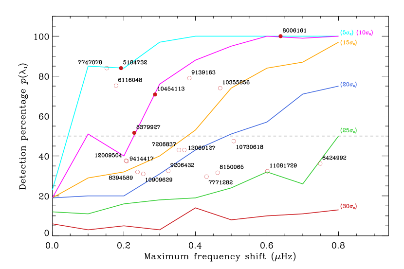
Figure 1: Detection percentage $p(\lambda_{1})$ as a function of the maximum linear frequency shift $\lvert\textrm{Max}(\delta\nu)\rvert_{\textrm{L}}$ obtained from 100 realizations of each simulated spectrum (see Section 4.2). Each solid line corresponds to a given (color-coded) level of noise $\sigma_{0}$. The opened red circles correspond to the Kepler stars which successfully passed the selection criterion $\lambda_{1}$, while the filled red circles indicate the stars which passed the selection criterion $\lambda_{2}$ as well (see Section 5). The $y$ coordinate of each star represents the percentage $p(\lambda_{1})$ of being detected according to the simulations. The horizontal dashed line indicates the 50% detection threshold.

Table 3: Detection percentage $p(\lambda_{2})$ to have the selection criterion $\lambda_{2}$ fulfilled, based on simulations of sinusoidal varying frequency shifts. The results for simulated periodicity of 4 years are presented here.

	$\overline{\sigma_{\delta\nu}}$ ($\mu$Hz)
	0.09	0.16	0.25	0.35	0.61	0.70
$\delta\nu^{\textrm{cycle}}$ ($\mu$Hz)
0.0	5	9	9	5	2	0
0.2	97	50	19	6	3	0
0.3	100	84	38	21	2	0
0.4	100	100	69	29	7	0

4.1 Simulations with the photometric VIRGO data

The selection criteria $\lambda_{1}$ and $\lambda_{2}$ were characterized through Monte-Carlo simulations using 4 years of photometric space-based observations of the Sun collected by the Sun Photometers (SPM) of the Variability of Solar Irradiance and Gravity Oscillations (VIRGO; Fröhlich et al., 1995) instrument on board the Solar and Heliospheric Observatory (SoHO; Domingo et al., 1995) satellite. The selected VIRGO/SPM time series, long of 1440 days, starts on February 8, 2007 and is centered around the deep and long minimum of the solar cycle 23 (e.g., Salabert et al., 2009). It was split into 16 subseries of 90 days, and the associated power spectra computed.

The outline of the Monte-Carlo simulations is the following: (1) a reference power spectrum was defined as the mean spectrum of the 16 VIRGO/SPM spectra; (2) starting from this reference spectrum, 16 power spectra were constructed by shifting their p-mode frequencies from one spectrum to the next in both a linear and sinusoidal ways; (3) finally, additional noise following a $\chi^{2}$ distribution and proportional to the photon noise, $\sigma_{0}$, estimated from the high-frequency region of the reference power spectrum was included to the power spectra. For validation purposes, we checked that the selection criteria do not return positive detections for variability of the frequency shifts extracted from the 16 VIRGO/SPM power spectra taken during solar minimum and used in the Monte-Carlo simulations.

4.2 Selection criterion $\lambda_{1}$

The absolute minimum-to-maximum temporal variations of the frequency shifts along the total duration of the observations, $\lvert\textrm{Max}(\delta\nu)\rvert_{\textrm{L}}$, is estimated from the linear regression of the temporal variations of the extracted frequency shifts, $\delta\nu(t)$. The selection criterion $\lambda_{1}$ is fulfilled when:

$$\lvert\textrm{Max}(\delta\nu)\rvert_{\textrm{L}}>\overline{\sigma_{\delta\nu}},$$ (1)

where $\overline{\sigma_{\delta\nu}}$ corresponds to the mean value of the uncertainties on the extracted frequency shifts.

The criterion $\lambda_{1}$ was assessed through simulations of linear frequency shifts introduced in the 90-day-long VIRGO/SPM reference spectrum (see Section 4.1). Maximum frequency shifts $\delta\nu^{\textrm{max}}$ between 0.0 and 0.8 $\mu$Hz were modeled along the 16 contiguous spectra. Different frequency shifts were included by steps of 0.1 $\mu$Hz. All the p-mode frequencies were shifted by the same amount, meaning that no frequency dependence of the frequency shift was introduced. In addition, noise levels between 5$\sigma_{0}$ and 30$\sigma_{0}$ in steps of 5$\sigma_{0}$ were introduced, where $\sigma_{0}=0.4$ ppm. The frequency shifts of these simulated spectra were then extracted using Method #1 as described in Section 3.1.1. The mean errors on the frequency shifts, $\overline{\sigma_{\delta\nu}}$, extracted from the simulated spectra depend on the introduced level of noise and lie between 0.09 and 0.70 $\mu$Hz, which is comparable to the errors obtained with real data.

The results obtained for 100 realizations of each simulated spectrum are shown in Fig. 1, while Table 2 provides the corresponding detection percentage, $p(\lambda_{1})$, to have the criterion $\lambda_{1}$ fulfilled. Each line represents the number of successful detections as a function of a given level of noise. When no frequency shift was introduced, the numbers given in Table 2 represent the percentage of false positives, which ranges from 23% to 6%. These false positives are higher when the noise is lower. Indeed, any small shift created by the noise is likely to be larger than the mean error, $\overline{\sigma_{\delta\nu}}$, when this one is small. On the other hand, when the noise is low and the maximum frequency shift $\lvert\textrm{Max}(\delta\nu)\rvert_{\textrm{L}}$ is larger than 0.3 $\mu$Hz, the temporal variability of the p-mode frequency shifts is detected 100% of the time. We note that we checked that similar results were obtained if a larger number of realizations was used.

Table 4: List of stars fulfilling the selection criterion $\lambda_{1}$ for showing temporal variability of their p-mode frequency shifts.

KIC	$\lvert\textrm{Max}(\delta\nu)\rvert_{\textrm{L}}$	$\overline{\sigma_{\delta\nu}}$	$p(\lambda_{1})$	$\langle S_{\text{ph}}\rangle$	$P_{\text{rot}}$	Category
	($\mu$Hz)	($\mu$Hz)	(%)	(ppm)	(days)
5184732∗	0.192	0.077	84.0	222.0	19.79 $\pm$ 2.43	simple
6116048†	0.178	0.093	75.2	87.4	17.26 $\pm$ 1.96	simple
7206837	0.354	0.280	43.0	246.6	4.04 $\pm$ 0.28	simple
7747078	0.152	0.077	84.0	176.0	17.71 $\pm$ 1.78	mixed-modes
7771282	0.431	0.396	29.7	117.6	11.88 $\pm$ 0.91	F-like
8006161∗	0.638	0.131	100.0	763.5	29.79 $\pm$ 3.09	simple
8150065	0.462	0.400	31.6			simple
8379927∗,♭	0.229	0.138	51.6			simple
8394589	0.238	0.196	32.0			simple
8424992	0.749	0.449	36.2			simple
9139163‡	0.383	0.194	78.9			simple
9206432	0.324	0.297	32.6	96.7	8.80 $\pm$ 1.06	F-like
9414417	0.206	0.172	37.6	146.5	22.77 $\pm$ 2.37	F-like
10355856	0.469	0.227	74.0	321.5	4.47 $\pm$ 0.31	F-like
10454113∗	0.287	0.173	70.8	327.3	14.61 $\pm$ 1.09	simple
10730618	0.507	0.421	47.4			F-like
10909629	0.254	0.250	31.0	55.1	12.37 $\pm$ 1.22	F-like
11081729	0.601	0.521	32.3	272.2	2.74 $\pm$ 0.31	F-like
12009504	0.208	0.188	37.4	155.3	9.39 $\pm$ 0.68	simple
12069127	0.369	0.262	43.0	86.6	4.47 $\pm$ 0.31	F-like

4.3 Selection criterion $\lambda_{2}$

The differences between the 25% higher and lower percentiles of the extracted temporal variations of the frequency shifts $\delta\nu(t)$ provide a manner to evaluate the existence of variability shorter than the length of the observations, i.e. 4 years in the case of the Kepler satellite. The selection criterion $\lambda_{2}$ is thus defined to be fulfilled when:

$$[\delta\nu(t)^{25^{\textrm{th\_high}}}-\delta\nu(t)^{25^{\textrm{th\_low}}}]>3\times\overline{\sigma_{\delta\nu}},$$ (2)

where $\overline{\sigma_{\delta\nu}}$ corresponds to the mean errors on the extracted frequency shifts. It thus allows us to select stars showing sinusoidal behavior, i.e. cycle-like, of the frequency shifts, that could not be detected with the first criterion $\lambda_{1}$ defined to measure the linear deviation from zero of the frequency shifts over the total length of the observations.

To characterize the $\lambda_{2}$ criterion, sinusoidal frequency shifts were introduced with cycle amplitudes, $\delta\nu^{\textrm{cycle}}$, of 0.2, 0.3, and 0.4 $\mu$Hz and periods of 1, 2, 3, and 4 years in the VIRGO/SPM reference power spectrum (see Section 4.1). The same levels of noise as the ones applied in Section 4.2 were introduced. The frequency shifts of these simulated spectra were obtained using Method #1 as described in Section 3.1.1. The results obtained from 100 realizations of each simulated spectrum are shown in Table 3 which provides the corresponding detection percentage $p(\lambda_{2})$ to have the criterion $\lambda_{2}$ fulfilled. Table 3 was obtained for a simulated period of 4 years, and similar values are obtained for periods of 1, 2, and 3 years. The selection criterion $\lambda_{2}$ thus defined is quite restrictive. When the introduced noise produces mean errors on the frequency shifts $\overline{\sigma_{\delta\nu}}$ larger than 0.16 $\mu$Hz and that the introduced cycle amplitudes are smaller than 0.3 $\mu$Hz, less than 20% of the stars are recovered. On the other hand, the number of false positives is never higher than 10% in all the simulated cases. However, if the criterion $\lambda_{2}$ is relaxed to a threshold of $2\times\overline{\sigma_{\delta\nu}}$, the number of false positives becomes larger than 70%.

Figure 2: Temporal variability of the p-mode frequency shifts (in $\mu$Hz) extracted from the cross-correlation analysis (Method #1) of the solar-like pulsating Kepler stars fulfilling the selection criterion $\lambda_{1}$ (see Table 4).

4.4 Selection criterion $\lambda_{3}$

The $\lambda_{3}$ criterion checks the Spearman’s correlation coefficients, $r$, between the temporal variations of the extracted frequency shifts and the photometric activity proxy $S_{\textrm{ph}}(t)$ estimated with the contemporaneous Kepler LC data. The $S_{\textrm{ph}}(t)$ proxy was estimated for the stars with a known rotation period, $P_{\mathrm{rot}}$ (García et al., 2014a), over subseries of $5\times P_{\mathrm{rot}}$. The criterion $\lambda_{3}$ helps to recover stars having photospheric magnetic variability but that did not pass the criteria $\lambda_{1}$ and $\lambda_{2}$ because their large errors on the frequency shifts due to low signal-to-noise ratio of the p-mode oscillations. The selection criterion $\lambda_{3}$ was fulfilled when:

$$r[\delta\nu(t),S_{\textrm{ph}}(t)]>0.5$$ (3)

The $S_{\textrm{ph}}(t)$ proxy was thus interpolated to the same dates as the ones used to measure the frequency shifts (Method #1, subseries of 90 days). We note also that the coefficients $r$ were computed using independent points only.

5 Results

Out of the 87 stars in the initial sample defined in Section 2, 20 candidates (11 simple stars, 8 F-like stars, and 1 mixed-mode star; see Table 4) fulfill the selection criterion $\lambda_{1}$ for showing temporal variability of their frequency shifts. These stars were included in Fig. 1 by interpolating their maximum linear frequency shift $\lvert\textrm{Max}(\delta\nu)\rvert_{\textrm{L}}$ and their levels of noise. Their positions on the y-axis indicate their associated percentage, $p(\lambda_{1})$, of being detected according to the simulations (see Section 4.2 and Table 4). The corresponding mean values of the temporal evolution of the $S_{\text{ph}}(t)$ proxy (see Section 4.4), along the associated rotation periods, $P_{\textrm{rot}}$, used to compute them, are also given in Table 4.

Out of these 20 stars, 8 of them have a detection percentage $p(\lambda_{1})$ higher than 50$\%$. With the application of the selection criterion $\lambda_{2}$ (see Section 4.3), 4 stars are selected. These stars have a detection percentage $p(\lambda_{2})$ above 50% and an associated detection percentage of false positives lower than 10%, given their mean errors on the extracted frequency shifts $\overline{\sigma_{\delta\nu}}$ being smaller than 0.2 $\mu$Hz (Table 3 and Table 4). These 4 stars were also selected with the criterion $\lambda_{1}$.

Figure 2 shows the frequency shifts extracted from the cross-correlation analysis (Method #1) of the 20 stars fulfilling the selection criterion $\lambda_{1}$ (Table 4). Comparable results are obtained with the peak-fitting analysis (Method #2). The temporal variations and associated uncertainties are quite different from one star to the other, but all the shifts are within $\pm 1\mu$Hz over the duration of the Kepler mission. Some stars have very small errors of the shifts, such as KIC 5184731, KIC 6116048, and KIC 7747078. The stars KIC 7771282, KIC 8150065, KIC 8424992, KIC 10355856, KIC 10909629, and KIC 12069127, which were observed for less than three years show nonetheless signatures of frequency shifts. The star KIC 9139163, flagged in Table 4, has an interesting and well defined periodicity of the frequency shifts of about 385 days, which is surprisingly close to the Kepler orbital period. To evaluate the origin of such coinciding periodicity, any possible effects of the line-of-sight (Davies et al., 2014) and Earth-trailing orbit in the Kepler observations on the p-mode frequencies need to be investigated in more details.

The p-mode oscillations of F-like stars with short lifetimes result in broad linewidths in the spectral domain. The errors on the extracted frequency shifts of these stars are thus much larger than for the simple stars whose oscillations have longer lifetimes. Uncovering significant frequency shifts larger than their errors is then more difficult to achieve for F-like stars, although their shifts are expected to be larger than for the simple stars (Metcalfe et al., 2007). In consequence, except KIC 10355856, the 8 F-like stars selected with the criterion $\lambda_{1}$ have detection percentages lower than 50%. One evolved star with mixed modes, KIC 7747078, also shows evidence for frequency shifts. This particular case is discussed in the following Section 5.1.

Furthermore, we note that two stars, the F-like star KIC 3733735 (Régulo et al., 2016) and the simple star KIC 10644253 (Salabert et al., 2016), known to show changes in the acoustic frequencies correlated to the photospheric magnetic activity measured with the $S_{\textrm{ph}}$ proxy were not selected with the criteria $\lambda_{1}$ and $\lambda_{2}$. Indeed, the errors on the extracted frequency shifts of these stars are large due to the low signal-to-noise ratio of their p-mode oscillations. The combination of the two criteria $\lambda_{1}$ and $\lambda_{2}$ is very restrictive allowing us to select only the best candidates among a large sample of stars to perform a detailed study of their frequency shifts. The stars thus selected do not constitute a full set of the active solar-like stars observed by Kepler but the best candidates which fulfill these objective criteria. An exhaustive analysis of the temporal variations of the frequency shifts of all the Kepler solar-like pulsating stars will be presented in Santos et al. (in preparation).

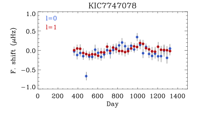
Figure 3: Temporal variability of the frequency shifts (in $\mu$Hz) of the individual $l=0$ (blue) and $l=1$ (red) modes measured for the evolved mixed-mode star KIC 7747078 extracted from the peak-fitting analysis (Method #2).

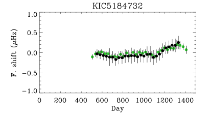
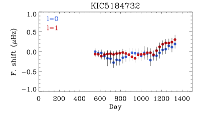
Figure 4: Upper-left panel: Comparison of the temporal variability of the frequency shifts (in $\mu$Hz) of KIC 5184732 extracted from the cross-correlation (Method #1, in green) and peak-fitting (Method #2, in black) analyses. Upper-right panel: Frequency shifts of the individual $l=0$ (blue) and $l=1$ (red) modes from Method #2. Bottom-left panel: Temporal variability of the photospheric activity proxy $S_{\textrm{ph}}$ (in ppm). Bottom-right panel: Frequency shifts extracted from Method #1 as a function of the photospheric magnetic proxy $S_{\textrm{ph}}$. The corresponding correlation coefficient $r$ and two-sided significance of the deviation from zero $p$ are also indicated.

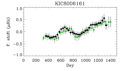
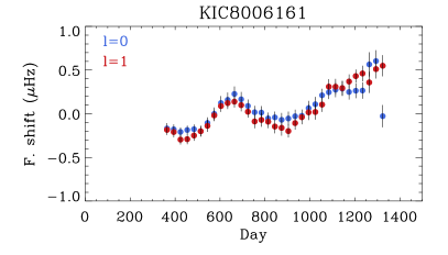
Figure 5: Upper-left panel: Comparison of the temporal variability of the frequency shifts (in $\mu$Hz) of KIC 8006161 extracted from the cross-correlation (Method #1, in green) and peak-fitting (Method #2, in black) analyses. Upper-right panel: Frequency shifts of the individual $l=0$ (blue) and $l=1$ (red) modes from Method #2. Bottom-left panel: Temporal variability of the photospheric activity proxy $S_{\textrm{ph}}$ (in ppm). Bottom-right panel: Frequency shifts extracted from Method #1 as a function of the photospheric magnetic proxy $S_{\textrm{ph}}$. The corresponding correlation coefficient $r$ and two-sided significance of the deviation from zero $p$ are also indicated.

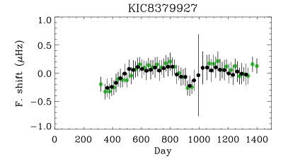
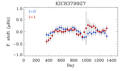
Figure 6: Left panel: Comparison of the temporal variability of the frequency shifts (in $\mu$Hz) of KIC 8379927 extracted from the cross-correlation (Method #1, in green) and peak-fitting (Method #2, in black) analyses. Right panel: Frequency shifts of the individual $l=0$ (blue) and $l=1$ (red) modes from Method #2.

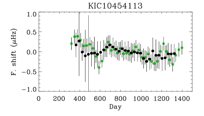
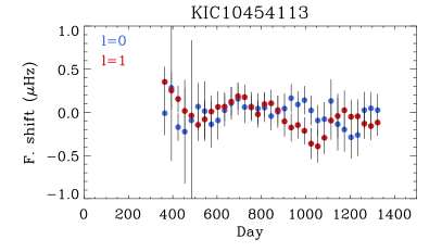
Figure 7: Left panel: Comparison of the temporal variability of the frequency shifts (in $\mu$Hz) of KIC 10454113 extracted from the cross-correlation (Method #1, in green) and peak-fitting (Method #2, in black) analyses. Right panel: Frequency shifts of the individual $l=0$ (blue) and $l=1$ (red) modes from Method #2.

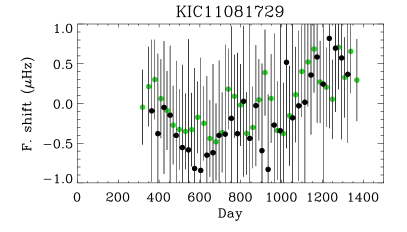
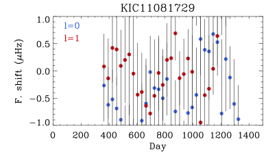
Figure 8: Upper-left panel: Comparison of the temporal variability of the frequency shifts (in $\mu$Hz) of KIC 11081729 extracted from the cross-correlation (Method #1, in green) and peak-fitting (Method #2, in black) analyses. Upper-right panel: Frequency shifts of the individual $l=0$ (blue) and $l=1$ (red) modes from Method #2. Bottom-left panel: Temporal variability of the photospheric activity proxy $S_{\textrm{ph}}$ (in ppm). Bottom-right panel: Frequency shifts extracted from Method #1 as a function of the photospheric magnetic proxy $S_{\textrm{ph}}$. The corresponding correlation coefficient $r$ and two-sided significance of the deviation from zero $p$ are also indicated.

5.1 Case of the more evolved star KIC 7747078

The star KIC 7747078 is the only star in our sample with mixed modes that fulfilled the selection criterion $\lambda_{1}$ with a detection percentage $p(\lambda_{1})$ of 84% indicating that frequency shifts are measured. In evolved stars with mixed modes, the $l=1$ modes do not follow the asymptotic relation and have usually low amplitudes. However, the $l=1$ mixed modes are well visible in KIC 7747078 (see e.g., Appourchaux et al., 2012) which allows us to extract precise frequency shifts. The individual frequency shifts of the $l=0$ and $l=1$ modes extracted from the peak-fitting analysis (Method #2) are shown in Fig. 3. The temporal variations of the mixed mode $l=1$ are interestingly comparable to the variations of the $l=0$ mode. Such unobserved behavior yet could bring new inferences for the study of magnetic field in more evolved stars than the Sun and will deserve a close look in the entire Kepler sample of evolved solar-like stars.

Table 5: Stars selected for a detailed analysis of the frequency dependence of their frequency shifts.

KIC	$\lambda_{1}$	$\lambda_{2}$	$\lambda_{3}$	$r$
5184732	*	*	*	0.52
8006161	*	*	*	0.71
8379927	*	*
10454113	*	*
11081729	*		*	0.72

5.2 Detailed analysis of the best stars

Based on Table 4, the subset of the most promising stars was selected for a detailed analysis of the frequency dependence of the frequency shifts using the peak-fitting results from Method #2. Indeed, in the case of the Sun, the frequency dependence (see e.g., Anguera Gubau et al., 1992; Chaplin et al., 1998; Salabert et al., 2004) provides inferences to differentiate among the possible physical mechanisms responsible for the frequency variations with the activity cycle (e.g., Gough, 1990).

This subset, given in Table 5, corresponds to the five stars which fulfill at least two of the selection criteria, $\lambda_{1}$, $\lambda_{2}$, and $\lambda_{3}$. Four of them are classified as simple stars (KIC 5184732, KIC 8006161, KIC 8379927, and KIC 10454113), and one as a F-like star (KIC 11081729). Although KIC 11081729 has a low detection percentage of 32%, which is typical for a F star, it has one of the largest frequency shifts among the selected stars (see Table 4), which is moreover well correlated with the $S_{\textrm{ph}}(t)$ proxy.

Figures 4, 5, 6, 7, and 8 show the comparison of the extracted frequency shifts between the cross-correlation analysis (Method #1) and the peak-fitting analysis (Method #2) for this subset of five stars. In the case of Method #2, the averaged values between the individual angular degrees $l=0$ and $l=1$ modes, as well as the individual $l=0$ and $l=1$ frequency shifts, are represented. When a surface rotation period $P_{\textrm{rot}}$ was measured, the temporal variation of the $S_{\textrm{ph}}(t)$ activity proxy interpolated over the same periods of time is also represented, along the relation between both observables. The Spearman’s correlation coefficients $r$ and the associated two-sided significances of the deviation from zero $p$ are also indicated on Figs. 4, 5, and 8, and in Table 5 too. We recall that these values were computed using independent points only.

Both methods #1 and #2, for which different lengths of subseries were used – 90 and 180 days respectively – are in excellent agreement with differences well within the uncertainties. For the simple stars, small differences between the frequency shifts of the individual $l=0$ and $l=1$ modes can be observed for KIC 5184732, KIC 8006161, and KIC 8379927, while larger disparity is present in KIC 10454113 along larger errors. Indeed, as well observed for the Sun, oscillation modes with different angular degrees respond differently to the activity cycle (see e.g., Pallé et al., 1989; Anguera Gubau et al., 1992; Howe et al., 1999; Jiménez-Reyes et al., 2001; Salabert et al., 2015, and references therein) in relation to the spatial distribution of the surface magnetic field (Howe et al., 2002; Jiménez-Reyes et al., 2004). This is what could be observed here for these stars. Again, the differences between the $l=0$ and $l=1$ modes for the F-like star KIC 11081729 are difficult to interpret given the large uncertainties.

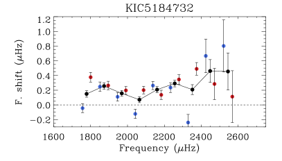
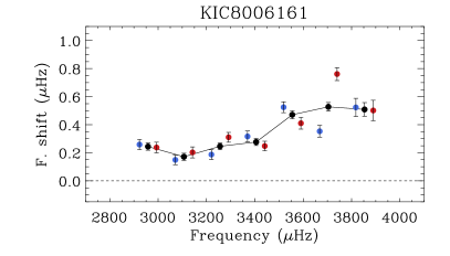
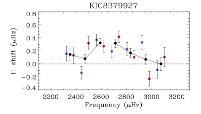
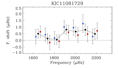
Figure 9: Frequency shifts of the individual $l=0$ (blue) and $l=1$ (red) modes as a function of frequency for KIC 5184732, KIC 8006161, KIC 8379927, and KIC 11081729 from Table 5. The black dots correspond to the averaged shifts between consecutive $l=0$ and $l=1$ modes. The horizontal dashed lines represent a zero shift.

In order to measure the frequency dependence of the frequency shifts, two periods of low and high activity around the median value of the frequency shifts were defined for each star. The weighted means of each fitted frequency from each 180-day subseries were estimated for both periods. The frequency shifts at each radial order were thus obtained by simply subtracting the frequencies measured during high activity by the corresponding frequencies at low activity. We considered both the $l=0$ and the $l=1$ modes independently. It is important to keep in mind that the two periods of activity thus defined are dependent on the unknown observed phase of magnetic variability for each given star. Despite this, the frequency dependence of the frequency shifts thus measured is found to be significant at $3\sigma$, $12\sigma$, $3\sigma$, and $2\sigma$ from the mean shift for KIC 5184732, KIC 8006161, KIC 8379927, and KIC 11081729 respectively, where $\sigma$ is the mean error on the shifts. This corresponds to confidence levels higher than 95%. However, although KIC 10454113 fulfills the criteria $\lambda_{1}$ and $\lambda_{2}$, no frequency dependence of the frequency shifts could be found at the level of precision of the data with a $1\sigma$ significance (i.e. a 68% confidence).

Figure 9 shows the frequency shifts as a function of frequency for KIC 5184732, KIC 8006161, KIC 8379927, and KIC 11081729. The shifts of the individual $l=0$ and $l=1$ modes are represented as well as the corresponding mean values. Except for KIC 8006161 which shows a frequency dependence comparable to what is observed in the case of the Sun (see e.g., Anguera Gubau et al., 1992; Chaplin et al., 1998; Salabert et al., 2004), as well as for KIC 10644253 (Salabert et al., 2016) and HD 49933 (Salabert et al., 2011), the three other stars, KIC 5184732, KIC 8379927, and KIC 11081729 follow quite different behaviors.

Table 6: Stellar parameters derived in Section 6 of the modeled stars.

KIC	$R$ $(R_{\odot})$	$M$ $(M_{\odot})$	Age (Gyr)	$T_{\rm{eff}}$ $(K)$	log $g$	[Fe/H]	$\tau_{\rm{HeII}}$ $(s)$
5184732	$1.37\pm 0.02$	$1.29\pm 0.04$	$4.00\pm 0.29$	$5870\pm 120$	$4.272\pm 0.005$	$+0.29\pm 0.20$	$916\pm 10$
8006161	$0.94\pm 0.01$	$1.01\pm 0.03$	$4.98\pm 0.17$	$5338\pm 66$	$4.497\pm 0.005$	$+0.64\pm 0.04$	$621\pm 10$
8379927	$1.14\pm 0.01$	$1.17\pm 0.03$	$1.55\pm 0.09$	$6045\pm 110$	$4.393\pm 0.003$	$-0.10\pm 0.15$	$683\pm 10$
11081729	$1.38\pm 0.01$	$1.27\pm 0.05$	$2.21\pm 0.07$	$6349\pm 28$	$4.261\pm 0.011$	$+0.11\pm 0.10$	$798\pm 10$

6 Discussion

The degree dependence of the frequency shifts observed in the Sun from the low- to high-degree angular modes is removed once the shifts are corrected by the mode inertia (see e.g., Libbrecht & Woodard, 1990; Chaplin et al., 2001; Howe et al., 2002). The shifts thus follow a smooth increase with frequency. This indicates that the structural changes occurring with magnetic activity that produce the p-mode frequency shifts are located in a thin layer close to the surface. Different observational and theoretical works were carried out in order to better understand the observed dependences of the frequency shifts (see e.g., Basu, 2016, for a review). For instance, the frequency dependence through the activity cycle was shown to be consistent with a decrease of less than 2% in the radial component of the turbulent velocity in the outer layers of the Sun (Kuhn & Schüssler, 2000; Dziembowski et al., 2001; Dziembowski & Goode, 2005). This mechanism is only efficient in the uppermost layers of the convective zone where the turbulent velocities become comparable to the local sound speed and explains the smooth increase of the shifts with frequency.

Nonetheless, detailed analyses of the frequency dependence of the p-mode frequency changes with magnetic activity in the Sun revealed further information. Indeed, Goldreich et al. (1991) first drew the attention of an apparent oscillatory component superimposed on the dominant smooth frequency trend of the frequency shifts. Based on the period of the signal, the authors surmised that it could be caused by changes in the magnetic field with the solar activity cycle confined to a thin layer just above the He i ionization zone. Gough (1994) estimated that the period of this oscillatory feature was roughly twice the inverse of the acoustic depth of the He ii ionization zone. He thus proposed to relate this oscillatory feature with a temporal variation in the depression of the first adiabatic exponent located in a deeper layer than Goldreich et al. (1991) had suggested, and to associate it with changes in the acoustic glitch caused by the He ii ionization. Basu & Mandel (2004) and Verner et al. (2006) did also detected variations with activity in the amplitude of the He ii acoustic glitch. However, the physical mechanism responsible for such periodic changes is still not clear. See Gough (2013) for a more detailed discussion.

Moreover, helioseismic inversions using the Michelson Doppler Imager (MDI; Scherrer et al., 1995) observations on board the SoHO satellite provided inferences on the radial dependence of the sound speed variations between the solar maximum and minimum (Baldner & Basu, 2008; Rabello-Soares, 2012). Mullan et al. (2012) compared their results with the sound speed changes expected from a model of magnetic inhibition of convective onset and found an agreement for at least the outer half of the convection zone. Since these structural inversions require intermediate- and high-degree modes, such detailed analysis is unfortunately not possible for other stars than the Sun. However, we can compare the frequency dependence between the stars discussed in Section 5.2 once their shifts are corrected by their mode inertia in relation to what it is observed in the Sun.

The mode inertia was obtained from structural models computed with MESA (Paxton et al., 2011). The OPAL opacities (Iglesias & Rogers, 1996) and the GS98 metallicity mixture (Grevesse & Sauval, 1998) were used, and the microscopic diffusion of elements was included, otherwise the standard input physics from MESA was applied. The theoretical low-degree, p-mode frequencies were computed in the adiabatic approximation using the ADIPLS code (Christensen-Dalsgaard, 2008). A $\chi^{2}$ minimization including simultaneously p-mode frequencies and spectroscopic data was applied. The procedure is comparable to the one described in Pérez Hernández et al. (2016), except that no gravity-like mixed modes were considered here. The input spectroscopic parameters such as, effective temperature ($T_{\rm{eff}}$), surface gravity ($\log g$), metallicity ([Fe/H]), and luminosity which was derived from the Hipparcos and Gaia parallaxes, were retrieved from the SIMBAD astronomical database. The stellar parameters thus obtained (see Table 6) are consistent with the inputs parameters and are comparable to those found by Metcalfe et al. (2014), Creevey et al. (2017), and Silva Aguirre et al. (2017).

We then followed Salabert et al. (2016) and used the normalized frequency shifts defined as $(I_{n,l}/I_{\textrm{max}})\times\delta\nu_{n,l}/\nu_{n,l}\times\nu_{\mathrm{max}}$, where $I_{n,l}$ is the mode inertia and $I_{\textrm{max}}$ the mode inertia interpolated at the frequency $\nu_{\textrm{max}}$ of the maximum oscillation power excess. The scaling with $\nu_{\mathrm{max}}$ was introduced as it is linearly related to the acoustic cut-off frequency (Belkacem et al., 2011). To minimize the errors, the mean values of the frequency shifts between adjacent $l=0$ and $l=1$ modes were considered here. The normalized frequency shifts thus corrected by the mode inertia are shown in Fig. 10 as a function of $\nu/\nu_{\mathrm{max}}$ for each star in Table 5. For the Sun, the frequency dependence can be described by a polynomial of the form $\delta\nu\propto\nu^{\alpha}$, with $1\leq\alpha\leq 2$ (Salabert et al., 2016). The horizontal dotted lines in Fig. 10 correspond to $\alpha=1$ and the blue dashed lines to $\alpha=2$. The mean normalized frequency shifts ($\alpha=1$) are estimated to be 0.22, 0.46, 0.20, and $0.56\,\mu$Hz for KIC 5184732, KIC 8006161, KIC 8379927, and KIC 11081729 respectively. For comparison, the corresponding value for the Sun is $0.24\,\mu$Hz.

Nonetheless, Fig. 10 suggests that a linear formulation of the frequency dependence of the normalized frequency shifts is not sufficient to properly describe the variations within their uncertainties. Such discrepancies could indicate the presence of an additional or a different source of frequency perturbation. If the frequency perturbation caused by structural changes arises from a thin layer inside the resonant cavity of the acoustic modes, the frequency dependence of the frequency shifts will then follow a sinusoidal function of the form $A\cos(\omega 2\tau+\varphi)$, where $\omega=2\pi\nu$ is the p-mode angular frequency and $\tau$ the acoustic depth of the perturbation. The variables $A$ and $\varphi$ correspond to the amplitude and the phase of the sine wave respectively. The minimization of this sinusoidal function was performed by fitting the parameters $A$ and $\varphi$ as well as an additional offset to take into account the non-zero mean of the shifts. We tried also to fit the parameter $\tau$, but given the small number of measurements for each star and their associated errors, the determination of the acoustic depth of an hypothetic oscillatory signal from a non-linear fit depends strongly on its initial value. Therefore, $\tau$ was kept fixed and only the other parameters were varied. In order to have a reference to represent the sine-wave dependence of the normalized frequency shifts for each star, the parameter $\tau$ was fixed to the acoustic depth of the He ii ionization zone $\tau_{\textrm{He{ii}}}$ given in Table 6. This choice appears natural because, as mentioned earlier on, there are observational evidences of such oscillatory feature in the frequency shifts of the Sun (see e.g., Goldreich et al., 1991; Gough, 1994, 2013), even though its amplitude is much smaller than the main trend. The corresponding fits thus obtained are represented in Fig. 10 by the red solid lines. It is interesting to notice that as a first approximation the use of the He ii acoustic depth can reproduce the observed dependence of the normalized frequency shifts.

Such oscillatory behavior could suggest that the perturbations of the turbulent velocity in the outer layers, which is the main cause of the frequency shifts observed in the case of the Sun, is not the dominant factor in the four stars analyzed here and that it could be located within the resonant cavity instead. Given the quality of the data and the small number of stars which successfully passed our selection criteria, this is an intriguing hypothesis which would need to be investigated with a larger number of solar-like stars observed for instance in the future by the PLATO space mission (Rauer et al., 2014).

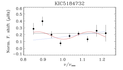
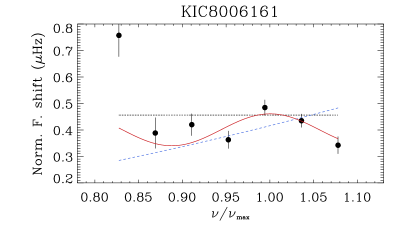
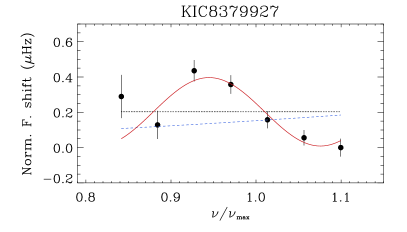
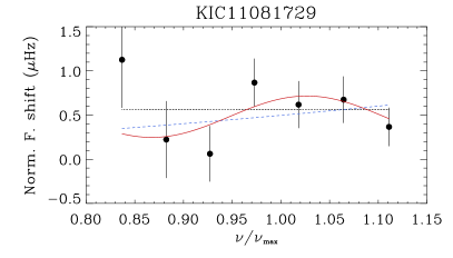
Figure 10: Normalized frequency shifts corrected by the mode inertia as a function of $\nu/\nu_{\mathrm{max}}$ for KIC 5184732, KIC 8006161, KIC 8379927, and KIC 11081729 as discussed in Section 6. The polynomial descriptions of the frequency shifts are represented by the horizontal dotted lines for $\alpha=1$ and by the blue dashed lines for $\alpha=2$. The solid red lines correspond to the results from the sine-wave fitting.

7 Conclusions

The photometric Kepler observations of a sample of 87 main-sequence, solar-like pulsating stars were analyzed in order to study their magnetism through the measurements of their p-mode frequency shifts, obtained using two independent methods: a cross-correlation analysis of all the visible modes, and a peak-fitting analysis of the individual modes. The results from both methods were compared to each other and to the associated photometric activity proxy $S_{\text{ph}}$ as well. To determine if the measured variations are likely to be genuine signatures of magnetic variability or to be noise, we developed restrictive selection criteria based on Monte Carlo simulations. A subset of 20 stars was thus selected as potential candidates, for which the frequency dependence of the individual $l=0$ and $l=1$ frequency shifts was measured for the four best stars fulfilling the selection criteria. We used the normalized frequency shifts corrected by the mode inertia to study the frequency dependence of the shifts in relation to what is known for the Sun. Although the sample is small and the uncertainties large to derive firm conclusions, the results obtained here could suggest that the dominant source of the perturbation responsible for the frequency shifts with magnetic activity in these four stars is different than in the Sun.

Furthermore, within this subset of 20 potential candidates, the frequency shifts of the $l=1$ modes of a more evolved star with mixed modes were observed to be comparable to the $l=0$ frequency shifts.

Appendix A Temporal variability of the mode power and damping in KIC 5184732 and KIC 8006161

In this Appendix, we present the temporal variability of the p-mode heights and linewidths extracted from the peak-fitting analysis (Method #2, Section 3.1.2) for two stars, KIC 5184732 and KIC 8006161. The mode power and energy supply rate were also estimated as described in Salabert & Jiménez-Reyes (2006). These two stars are the most promising stars in our sample for showing variations in other p-mode parameters than frequencies.

Figures 11 and 12 show the fractional temporal evolutions likely associated to magnetic activity of the mode heights, linewidths, powers, and energy supply rates of KIC 5184732 and KIC 8006161 respectively. They are compared to the corresponding variations of the background noise and of the duty cycle of the analyzed Kepler subseries. The relations between mode heights and linewidths with the frequency shifts are also shown on Fig. 11 and 12. The associated Spearman’s correlation coefficients $r$ and two-sided significances of the deviation from zero $p$ are given as well. We note that they were computed using independent points only. Finally, the relations between the background noise and the mode heights are presented. The results between correlation and anti-correlation of the variations with magnetic activity are similar to what is observed for the Sun. In the case of KIC 8006161, we confirm the results from Kiefer et al. (2017) on the anti-correlation between the frequency shifts and the mode height variability.

Figure 13 shows the frequency dependence of the mode height and linewidth variabilities. Although the results are clearer for KIC 8006161, the observed dependences are comparable to what observed in the Sun (see e.g., Salabert & Jiménez-Reyes, 2006). It is the first time that such a frequency dependence of the mode heights and linewidths with magnetic activity is observed in distant stars.

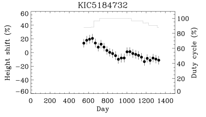
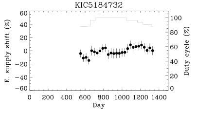
Figure 11: Fractional temporal variability (in %) of the p-mode power and damping parameters extracted from the peak-fitting analysis (Method #2) of KIC 5184732. The duty cycle is shown in light grey. The corresponding correlation coefficients $r$ and two-sided significances of the deviation from zero $p$ are also indicated.

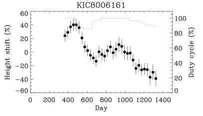
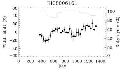
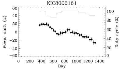
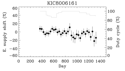
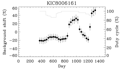
Figure 12: Fractional temporal variability (%) of the p-mode power and damping parameters extracted from the peak-fitting analysis (Method #2) of KIC 8006161. The duty cycle is shown in light grey. The corresponding correlation coefficients $r$ and two-sided significance of the deviation from zero $p$ are also indicated.

Figure 13: Frequency dependence of the fractional variations measured in the p-mode heights and linewidths of KIC 5184732 (top) and KIC 8006161 (bottom). The horizontal dashed lines represent a null variation.