The dynamics of the de Sitter resonance

Abstract.

We study the dynamics of the de Sitter resonance, namely the stable equilibrium configuration of the first three Galilean satellites. We clarify the relation between this family of configurations and the more general Laplace resonant states. In order to describe the dynamics around the de Sitter stable equilibrium, a one-degree of freedom Hamiltonian normal form is constructed and exploited to identify initial conditions leading to the two families.

The normal form Hamiltonian is used to check the accuracy in the location of the equilibrium positions. Besides, it gives a measure of how sensitive it is with respect to the different perturbations acting on the system. By looking at the phase-plane of the normal form, we can identify a Laplace-like configuration, which highlights many substantial aspects of the observed one.

1. Introduction

The three Galilean satellites of Jupiter, Io, Europa and Ganymede are phase-locked in the so-called Laplace resonance [FM79, MD99]. This fascinating dynamical state involves the commensurability 4:2:1 of the mean motions and a locking of the relative precession of the peri-Jove of Io and Europa. On the other hand, the peri-Jove of Ganymede is not locked: hence, out of the four resonant angles combining longitudes and arguments of peri-Joves, three are librating and one is rotating [SM97].

However, a state in which all four combination angles are librating is conceivable and indeed dynamically possible. Its discovery is usually attributed to de Sitter [dS31] and is actually only one of a possible set of dynamical states [BH16]. In a simplified planar model of the mutual interactions of the three satellites in the Newtonian field of Jupiter, after reducing to four degrees of freedom, the de Sitter dynamical states are indeed equilibrium points. In the four degrees of freedom model, the Laplace state corresponds to a periodic orbit in which three angles are fixed and a fourth angle changes periodically. The dynamics become quasi-periodic in the full system with six degrees of freedom. We refer to the de Sitter state as the only stable equilibrium in all four angular variables.

The starting model considered by de Sitter in [dS31] is the planar 4-body problem Jupiter-Io-Europa-Ganymede, in which the influence of Callisto and the Sun is neglected. There, he considers periodic orbits of $1^{st}$ and $2^{nd}$ kind, whose solutions, according to [Poi99], are circles or ellipses. In [dS31] de Sitter proves the existence of a family of periodic orbits with nearly circular Keplerian ellipses, parameterized by the eccentricity of one of the satellites. The seminal work of de Sitter was recently re-considered in [BZ17, BH16]. In both works, a 5-body problem including Callisto is considered. The existence of a positive measure set of Lagrangian invariant tori is proved to exist in a neighborhood of the periodic orbits.

In the present work we consider the 4-body problem Jupiter-Io-Europa-Ganymede. This system is described by a Hamiltonian function with 8 degrees of freedom (hereafter, DOF), which can be reduced to 6 DOF due to the translational symmetry. Following [Hen84, Mal91], we make a transformation of coordinates, taking into account the linear combinations of the angles corresponding to the Laplace resonance. It turns out that two variables are cyclic, thus reducing the model to a 4-DOF Hamiltonian. We then locate the stable equilibria of this system. By means of the Lie transform method, we construct a resonant normal form for the Laplace resonance. With this procedure we obtain an approximation of the Hamiltonian (namely, an expansion around reference values up to second order in the momenta), which allows us to reduce the problem to a 1-DOF Hamiltonian. In this context, we aim at clarifying the interrelationship between the two dynamical states (de Sitter and Laplace) which can be viewed as explicit solutions of the 1-DOF Hamiltonian system, whose normal form has the appearance of a fundamental resonance problem. On the phase-cylinder of this Hamiltonian, the de Sitter stable equilibrium is an elliptic fixed point. The libration domain around it is bounded by a critical curve beyond which rotating solutions exist (compare with Fig.1). One of these rotating trajectories is a fairly good approximation of the actual observed Laplace state. The reconstruction of the dynamics is quite accurate when also a first-order secular description of the oblate potential of Jupiter is included in the model.

Hamiltonian normal forms obtained in this framework are prototypes for the description of systems trapped in resonance. This de Sitter normal form can be used to explore the dynamics both around the librating and rotating regimes when perturbed with higher-degree terms in the expansions of the satellite mutual interactions, secular effects from Callisto, the Sun, higher-degree multipoles of Jupiter, etc. A further improvement of the model, which can be the subject of a future work, might include dissipative perturbations due to tidal interactions.

We illustrate the use of the 1-DOF Hamiltonian to check the accuracy in the location of the equilibrium and how sensitive is this when changing the nature of the perturbation. As an application, an inspection of the phase-plane of the normal form allows us very easily to identify a Laplace-like configuration which displays almost every feature of the observed one.

The plan of the paper is as follows: in Section 2 we introduce the Hamiltonian model; in Section 3 we locate the stable de Sitter equilibrium and construct the normal form; in Section 4 we investigate its predictive power and the sensitivity to higher-order effects and in Section 5 we discuss possible extensions and conclusions.

2. An analytical model of the Laplace resonance

We illustrate the analytic model based on the Hamiltonian method to reconstruct the dynamics around the Laplace resonance. We follow the standard approach of Henrard and Malhotra [Hen84, Mal91]. The model includes the most relevant interaction and can be conveniently generalized when inserting less important effects. Working in the Jacobi coordinate frame and considering only planar orbits, we take into account the Newtonian monopole, the oblateness of Jupiter and the mutual interaction of the three satellites (Io, Europa and Ganymede) involved in the resonance. Their osculating elements, respectively the semi-major axes, eccentricities, mean longitudes and longitudes of peri-Jove, are denoted as $\{a_{k},e_{k},\lambda_{k},\varpi_{k}\}$ with $k=1,2,3$.

The Newtonian monopole Hamiltonian is given by

$$H_{Kep}=-{{Gm_{0}m_{1}}\over{2a_{1}}}-{{G(m_{0}+m_{1})m_{2}}\over{2a_{2}}}-{{G(m_{0}+m_{1}+m_{2})m_{3}}\over{2a_{3}}}\ ,$$ (2.1)

where $m_{0},m_{k}\,(k=1,2,3)$ are, in order, the masses of Jupiter, Io, Europa and Ganymede.

The secular $J_{2}$-term in the oblate potential of Jupiter is

$$H_{J_{2}}=-{{Gm_{0}J_{2}R_{\jupiter}^{2}}\over{2}}\ \left[{m_{1}\over a_{1}^{3}}\left(1+{3\over 2}e_{1}^{2}\right)+{m_{1}+m_{2}\over a_{2}^{3}}\left(1+{3\over 2}e_{2}^{2}\right)+{m_{1}+m_{2}+m_{3}\over a_{3}^{3}}\left(1+{3\over 2}e_{3}^{2}\right)\right]\ ,$$ (2.2)

where $J_{2}=1.4736\times 10^{-2}$ is the Jupiter quadrupole coefficient in the multipole expansion of the gravitational potential and $R_{\jupiter}=71398$ kilometers is its equatorial radius. From the amount of these quantities we can state that the oblateness of Jupiter produces a very large effect, absolutely not negligible even in a first order picture: in fact the precession of peri-Joves turns out to be comparable in magnitude to the effects due to satellite couplings.

The mutual interaction of the three resonant satellites, limiting the expansion up to first order in the eccentricities, is given by:

$$H_{Sat} = -{{Gm_{1}m_{2}}\over a_{2}}\left\{{B_{0}}\left(\alpha_{12}\right)+\gamma_{1}\left(\alpha_{12}\right)e_{1}\cos(2\lambda_{2}-\lambda_{1}-\varpi_{1})+\gamma_{2}\left(\alpha_{12}\right)e_{2}\cos(2\lambda_{2}-\lambda_{1}-\varpi_{2})\right\}\$$ (2.3)

$$-{{Gm_{2}m_{3}}\over a_{3}}\left\{{B_{0}}\left(\alpha_{23}\right)+\gamma_{1}\left(\alpha_{23}\right)e_{2}\cos(2\lambda_{3}-\lambda_{2}-\varpi_{2})+\gamma_{2}\left(\alpha_{23}\right)e_{3}\cos(2\lambda_{3}-\lambda_{2}-\varpi_{3})\right\}\$$

$$-{{Gm_{1}m_{3}}\over a_{3}}\left\{{B_{0}}\left(\alpha_{13}\right)\right\}+{\rm O}(e_{k}^{2})\ ,$$

where the ${B_{0}}$ and $\gamma_{k}$ are defined as

$$B_{0}(\alpha)=\frac{1}{2}{b_{1/2}^{(0)}(\alpha)}-1,\quad\gamma_{1}(\alpha)={1\over 2}\left(4+\alpha{d\over{d\alpha}}\right)b_{1/2}^{(2)}(\alpha),\quad\gamma_{2}(\alpha)=-{1\over 2}\left(3+\alpha{d\over{d\alpha}}\right)b_{1/2}^{(1)}(\alpha)+2\alpha$$ (2.4)

and the $b_{s}^{(j)}(\alpha)$ are the Laplace coefficients [MD99] with $\alpha_{ik},(i,k=1,2,3)$ being $\alpha_{12}=a_{1}/a_{2}$, $\alpha_{23}=a_{2}/a_{3}$ or $\alpha_{13}=a_{1}/a_{3}$; indirect terms are included in the computation of the coefficients.

Since the eccentricities are small, it is convenient to use the modified Delaunay variables

$$L_{i}=\mu_{i}\sqrt{GM_{i}a_{i}}\ ,\qquad\widetilde{P}_{i}=L_{i}\left(1-\sqrt{1-e_{i}^{2}}\right)$$ (2.5)

with conjugate angles $\lambda_{i}$ and $p_{i}=-\varpi_{i}$. In these definitions, the following combinations of masses are introduced complying with the choice of the Jacobi frame:

$$M_{1} = m_{0}+m_{1}\ ,$$ (2.6)

$$M_{2} = m_{0}+m_{1}+m_{2}\ ,$$ (2.7)

$$M_{3} = m_{0}+m_{1}+m_{2}+m_{3}\ ,$$ (2.8)

$$\mu_{1} = \frac{m_{0}m_{1}}{M_{1}}\ ,$$ (2.9)

$$\mu_{2} = \frac{M_{1}m_{2}}{M_{2}}\ ,$$ (2.10)

$$\mu_{3} = \frac{M_{2}m_{3}}{M_{3}}\ .$$ (2.11)

Overall, we have the Hamiltonian function

$$H_{A}(L_{i},\widetilde{P}_{i},\lambda_{i},p_{i})=H_{Kep}+H_{J_{2}}+H_{Sat},\;\,i=1,2,3\ .$$ (2.12)

In order to exploit the resonances, we use the following Henrard-Malhotra coordinate transformation [Hen84, Mal91], which takes into account the resonant combinations of the angles corresponding to the Laplace resonance:

$$q_{1} = 2\lambda_{2}-\lambda_{1}+p_{1}\ ,\quad\quad P_{1}=\widetilde{P}_{1}\ ,$$ (2.13)

$$q_{2} = 2\lambda_{2}-\lambda_{1}+p_{2}\ ,\quad\quad P_{2}=\widetilde{P}_{2}\ ,$$ (2.14)

$$q_{3} = 2\lambda_{3}-\lambda_{2}+p_{3}\ ,\quad\quad P_{3}=\widetilde{P}_{3}\ ,$$ (2.15)

$$q_{4} = 3\lambda_{2}-2\lambda_{3}-\lambda_{1}\ ,\quad\;P_{4}={\scriptstyle{\frac{1}{3}}}\left(L_{2}-2(\widetilde{P}_{1}+\widetilde{P}_{2})+\widetilde{P}_{3}\right)\ ,$$ (2.16)

$$q_{5} = \lambda_{1}-\lambda_{3}\ ,\quad\quad\quad\quad\;\;P_{5}={\scriptstyle{\frac{1}{3}}}\left(3L_{1}+L_{2}+\widetilde{P}_{1}+\widetilde{P}_{2}+\widetilde{P}_{3}\right)\ ,$$ (2.17)

$$q_{6} = \lambda_{3}\ ,\quad\quad\quad\quad\quad\quad\;\;\;P_{6}=L_{1}+L_{2}+L_{3}-\widetilde{P}_{1}-\widetilde{P}_{2}-\widetilde{P}_{3}$$ (2.18)

and, for sake of convenience, we also give the list of the old $L$-actions in terms of the new ones

$$L_{1} = P_{5}-P_{4}-P_{1}-P_{2}\ ,$$ (2.19)

$$L_{2} = 3P_{4}+2P_{1}+2P_{2}-P_{3}\ ,$$ (2.20)

$$L_{3} = P_{6}-P_{5}-2P_{4}+2P_{3}\ .$$ (2.21)

In this way we obtain the transformed Hamiltonian

$$H_{B}(P_{\alpha},q_{a})=H_{A}\left(L_{i}(P_{\alpha}),P_{i},\lambda_{i}(q_{\alpha}),p_{i}(q_{\alpha})\right),\;\alpha=1,...,6,\quad a=1,...,4\ ,$$ (2.22)

whose explicit form is given in Appendix A, formula (A). Now, the relevant property of (A) is that $q_{5}$ and $q_{6}$ are cyclic in $H_{B}$, so that $P_{5}$ and $P_{6}$ are integrals of motion. Therefore we get a 4-DOF Hamiltonian system with $P_{5}$ and $P_{6}$ as parameters.

Henrard [Hen84] and Malhotra [Mal91], in their respective Hamiltonian models, proceed to expand the function around reference values for $P_{4},P_{5},P_{6}$, noticing that they are intrinsically large quantities when compared with $P_{1},P_{2},P_{3}$. To preserve the accuracy in the following computations, we prefer at the moment not to perform this expansion. However, we will exploit these reference values as seeds for the computation of the equilibria. Moreover, since it is large but not conserved, we split the momentum $P_{4}$ according to

$$P_{4}=\overline{P}_{4}+\delta P_{4}\ ,$$ (2.23)

where $\overline{P}_{4}$, defined below in (3.7), is a fixed value and $\delta P_{4}$ denotes a small variation. The 4-DOF system generated by $H_{B}$ is still quite complicated (and most probably non-integrable). We proceed by investigating its equilibria and the dynamics around them.

3. The de Sitter equilibrium

We recall that the Laplace resonance is a three-body orbital resonance involving the Jovian moons described by the relations

$$2\lambda_{2}-\lambda_{1}-\varpi_{1} = 0\ ,$$

$$2\lambda_{2}-\lambda_{1}-\varpi_{2} = \pi\ ,$$

$$2\lambda_{3}-\lambda_{2}-\varpi_{2} = 0\ .$$ (3.1)

As a consequence, the resonant Laplace argument $\phi_{L}$, defined by

$$\phi_{L}\equiv\lambda_{1}-3\lambda_{2}+2\lambda_{3}\ ,$$

librates around $\pi$: this implies that there can never be a triple conjunction of Io, Europa and Ganymede.

On the other side, the de Sitter equilibrium [dS31, BH16] corresponds to the set of relations:

$$q_{1} = 2\lambda_{2}-\lambda_{1}-\varpi_{1}=0\ ,$$ (3.2)

$$q_{2} = 2\lambda_{2}-\lambda_{1}-\varpi_{2}=\pi\ ,$$ (3.3)

$$q_{3} = 2\lambda_{3}-\lambda_{2}-\varpi_{3}=\pi\ ,$$ (3.4)

$$q_{4} = 3\lambda_{2}-2\lambda_{3}-\lambda_{1}(=-\phi_{L})=\pi\ .$$ (3.5)

We remark that these relations identify only one particular equilibrium state and that, as a matter of fact, several other equilibrium solutions are possible, each of them belonging to the de Sitter family (see [BH16]). By denoting with the sequence $\{0,\pi,\pi,\pi\}$ the values corresponding to (3.2)–(3.5), we can see that the combinations involving respectively one, two or three exchanges between $0$ and $\pi$, are still equilibria. Moreover, a rotation of the whole system by $\pi$, corresponding to an overall exchange of each $0$ with $\pi$ and of each $\pi$ with $0$, provides an additional set of eight equilibria. We have therefore a collection of 16 possible de Sitter equilibria. However, as found by Hadjidemetriou and Michalodimitrakis [HM81] and analytically checked in the works by Broer and Hanßmann [BH16] and Broer and Zhao [BZ17], all of them are linearly unstable, but for the one identified by (3.2)–(3.5) and its rotated counterpart. To this linearly stable configuration and the corresponding equilibrium value of the momenta, we will henceforth refer as the de Sitter equilibrium. We remark that these last equilibrium values are slightly displaced when adding to the Hamiltonian (2.22) a small perturbation sharing its symmetries with respect to the angles. Since the precise evaluation of these displacements can be difficult, we will generically have small librations around the given reference values of the combination angles.

Concerning the de Sitter equilibrium, the essential difference with respect to the standard Laplace resonant configuration is that, in addition to the conditions in (3), we now also have (3.4), that is the libration of $q_{3}$ around $\pi$. Since observations indicate that $q_{3}$ is rotating [SM97], we realize that de Sitter equilibrium is not the observed configuration of the Galilean satellites. However, we can study under which conditions the real system fails to stay in this status.

To locate the equilibrium, we look for the solution of the system of equations

$${{\partial H_{B}(P_{\alpha},q_{a})}\over{\partial P_{b}}}\bigg{|}_{DS}=0,\quad\quad{{\partial H_{B}(P_{\alpha},q_{a})}\over{\partial q_{b}}}\bigg{|}_{DS}=0\ ,\;\alpha=1,...,6,\quad a,b=1,...,4\ ,$$ (3.6)

where the suffix DS means that the derivatives are computed at the values in (3.2)–(3.5). An exact general solution is difficult to get explicitly; most probably it could be obtained if $H_{B}$ is expanded as in [Hen84] and [Mal91] and retaining linear terms in the small momenta. We instead proceed by inserting the explicit values of the numerical parameters and exploiting the FindRoot function of mathematica®.

The values of the parameters are determined according to the following conventions. We scale physical units by choosing $Gm_{0}=1$ and $a_{1}=1$. Actually, this last choice is equivalent to scale distances by the semi-major axis of a virtual Io, which is taken as the nominal mean value coming from ephemerides. Analogously, the average observed values of $a_{2},a_{3}$ and of the three eccentricities, are used to initialize the computations: in Table 1 we list the values of the elements used in [LDV04] taken from the IMCCE, which will be used in the forthcoming computations. The true proper semi-major axes involved in the dynamical status are among the outcome of the procedure and will slightly differ from them. The values of the Laplace coefficients used in the model are those corresponding to the mean elements: in Table 2 we list their values for the ephemeridal figures of Table 1 (denoted as [LDV04]) and, for sake of comparison, with the ephemerides extracted from the NASA’s SPICE toolkit (denoted as [J2000]) and also with the values corresponding to the exact commensurability (last row), $\alpha_{12}=\alpha_{23}=2^{-2/3}$. The values of ${B_{0}}(\alpha_{13})$, not included in Table 2, are all very close (within the last displayed digit) to the common value $0.04266$.

$\rm{Element}$	Io	Europa	Ganymede
semi-major axis [km]	422030.686	671262.329	1070622.862
eccentricity	0.004165	0.009366	0.001500
orbital period   [d]	1.769137	3.551182	7.154554
mean motion   [∘/d]	203.4890	101.3747	50.3176
mass ratio   [$m_{k}/m_{0}$]	$4.70\times 10^{-5}$	$2.56\times 10^{-5}$	$7.84\times 10^{-5}$

Table 1. Mean orbital elements according to Lainey et al. [LDV04]

Using these values in the definitions (2.5) and in the transformed momenta (2.16)–(2.18), we compute the following seeds for $\overline{P}_{4}$ and the integrals of motion $P_{5},P_{6}$:

$$\overline{P}_{4}=0.2289560,\quad P_{5}=1.2289716,\quad P_{6}=4.3437055\ .$$ (3.7)

$\overline{P}_{4}$ is the value of $P_{4}$ for the ephemeridal elements. In this way, solving the system (3.6) we get the following solution for the de Sitter equilibrium:

$$P_{1}^{*} = 9.74805159\times 10^{-6}\ ,$$ (3.8)

$$P_{2}^{*} = 3.55566494\times 10^{-5}\ ,$$ (3.9)

$$P_{3}^{*} = 6.84513718\times 10^{-7}\ ,$$ (3.10)

$$\delta P_{4}^{*} = -7.29208631\times 10^{-6}\ .$$ (3.11)

From these values and those in (3.7), using (2.19)–(2.21) we also get

$$L_{1}^{*} = 0.99997729\ ,$$ (3.12)

$$L_{2}^{*} = 0.68693684\ ,$$ (3.13)

$$L_{3}^{*} = 2.65683739\ ,$$ (3.14)

from which, using again their definitions in (2.16)–(2.18), we can recompute the values of $P_{4},P_{5},P_{6}$ for consistency. The corresponding proper orbital elements are as follows:

$$a_{1}^{*} = 1.0000016\ ,$$ (3.15)

$$a_{2}^{*} = 1.5905229\ ,$$ (3.16)

$$a_{3}^{*} = 2.5368556\ ,$$ (3.17)

$$e_{1}^{*} = 0.0044155\ ,$$ (3.18)

$$e_{2}^{*} = 0.0101746\ ,$$ (3.19)

$$e_{3}^{*} = 0.0007178\ .$$ (3.20)

Comparing these values with the figures of Tables 1 and 2, we see that the new semi-major axis ratios are still very close to the original ones and that the only slight but substantial change is in the eccentricity of Ganymede.

semi-major axis ratio	${B_{0}}$	$\gamma_{1}$	$\gamma_{2}$
$\alpha_{12}=0.628712$ [LDV04]	0.129531	$-1.183999$	0.424936
$\alpha_{12}=0.628733$ [J2000]	0.129540	$-1.184091$	0.424985
$\alpha_{23}=0.626983$ [LDV04]	0.128561	$-1.174833$	0.420078
$\alpha_{23}=0.627044$ [J2000]	0.128600	$-1.175330$	0.420341
$\alpha=0.629961=2^{-2/3}$	0.130217	$-1.190494$	0.428390

Table 2. Laplace coefficients.

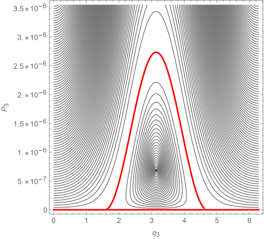
Figure 1. The normal form around the de Sitter equilibrium: the red curve represents the boundary which delimits the libration domain.

A normal form Hamiltonian can be constructed to describe the reduced dynamics around the de Sitter equilibrium, in much the same way as semi-analytical constructions have been performed to get expansion solutions [Bro77], making use of the advantages of the Lie-transform normalization [Kam70]. In order to apply the Lie-transform algorithm [Gio02, Eft11], we now expand the function $H_{B}$ around the solution values $P_{a}^{*}$ and keep terms up to second order in the momenta. This choice may at first seem to conflict with the first order expansion in the eccentricities. However, it is required to properly account for the relative importance of low-order non-resonant terms. The procedure to compute the normal form closely resembles the approach followed by Henrard [Hen84]: a sequence of near-identity canonical transformations is performed in order to remove selected terms in agreement with the specific aims of the normal form. Henrard’s aim was to leave only the Laplace argument and therefore to eliminate $q_{k},k=1,2,3$; instead, we are interested in the dynamics of the $(P_{3},q_{3})$ degree of freedom and therefore we eliminate the angles $q_{1},q_{2}$ and $q_{4}$. Therefore, by using the equilibrium values (3.8), (3.9) and $P_{4}^{*}=0.22894897$ computed from (2.16) and (3.11), we get a 1-DOF Hamiltonian depending on $P_{3}$ and $q_{3}$ with explicit form

$$H_{DS}(P_{3},q_{3})=-0.003728P_{3}-1.6495P_{3}^{2}-(6.1351\times 10^{-6}\sqrt{P_{3}}-1.1546\times 10^{-5}P_{3}^{3/2})\cos q_{3}\ .$$ (3.21)

The contour plot of this function, which is strictly related to the second fundamental resonance model introduced in [HL83], is displayed in Fig.1. The red curve represents the boundary which delimits the libration domain around the de Sitter equilibrium. The Laplace configuration is outside this domain, where the dynamics is rotational and $q_{3}$ ranges from 0 to $2\pi$. In this way we get a simple tool to highlight the reduced phase-space structure around the 4:2:1 resonance.

4. Integrations with the Hamiltonian model

We can exploit the plot of Fig.1 to investigate both the de Sitter stable libration and the actual Laplace state by locating suitable initial conditions.

Concerning the de Sitter equilibrium, we can at first ask two important questions: how precisely it is located by exactly evaluating the values of $P_{a}^{*}$ and how sensitive is this location with respect to higher-order effects. The first question arises from the fact that our computation is only in principle exact: two factors of uncertainties are given by the finite accuracy of the root-finding process and by the small inconsistency due to the fact that the Laplace coefficients used in the computations do not coincide with those corresponding to the elements of the solutions. The second question is instead more generally related to the global persistence of the equilibrium with respect to the reintroduction of all other perturbing effects excluded in the simplified model.

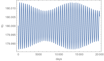
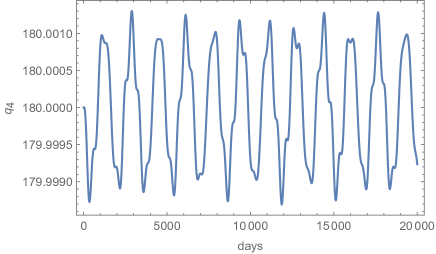
Figure 2. Uncertainty in the location of the de Sitter equilibrium: left, the libration of the $q_{3}$ combination; right, the libration of the Laplace angle (both angles are in degrees).

In Fig.2 we see the numerical solutions of the canonical equations given by the Hamiltonian $H_{B}$ with initial conditions corresponding to the de Sitter equilibrium. The fluctuations of the $q_{3}$ combination angle correspond to an uncertainty of order $10^{-4}$, that of the Laplace angle to $10^{-5}$. From the simulations, also the equilibrium values of the momenta $P_{a},a=1,...,4,$ fluctuate of the same amount ($10^{-4}$), whereas the integrals $P_{5},P_{6}$ are exactly conserved. These results are in substantial agreement with the expected variations of the values of the Laplace coefficients (cfr. Table 2): one could think to a refinement of the procedure with an iterative approach using updated values of the coefficients at each step.

Concerning higher-order effects, we have performed some investigations by extending the model with the addition of the following terms:

$\bullet$ the satellite self-interactions up to 2nd order in the eccentricities;

$\bullet$ the secular influence of Callisto and the Sun;

$\bullet$ the octupolar term in the expansion of the field of Jupiter.

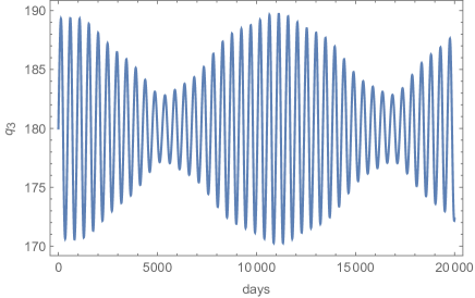
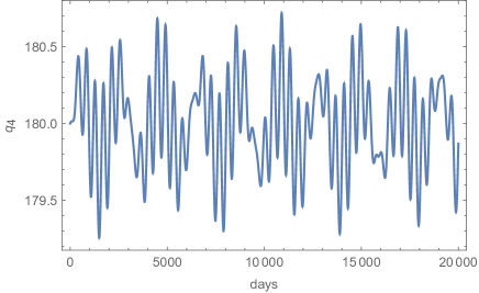
Figure 3. Persistence of the de Sitter equilibrium with respect to additional high-order effects (see text): left, the libration of the $q_{3}$ combination; right, the libration of the Laplace angle.

The expressions of these higher-order terms are written in Appendix B. In Fig.3 we see the numerical solutions of the canonical equations given by the second-order model Hamiltonian including the above effects starting with the same initial conditions as before. We see that the $q_{3}$ angle shows appreciable quasi-periodic oscillations, but well within the limit of the libration area; the Laplace angle has still a quite small amplitude of variation. Three time-scales emerge from the plots in Figg.2-3: a 485-days oscillation related to the 2:1 two commensurabilities (see the frequency value of (4.1) below), a $\sim 2000$-days oscillation in the Laplace argument and a low-frequency modulation, probably a beat between the two resonances.

Also in the real Laplace resonance, a very small amplitude of the librations of $q_{1},q_{2}$ and $q_{4}$ is usually reported [YP81]. We can conjecture that this status is in some sense close to that of the de Sitter equilibrium but not trapped at it. A reasonable assumption is that of choosing initial conditions for motion of the model system of the Hamiltonian $H_{B}(P_{\alpha},q_{\alpha})$ given by $P_{1}=P_{1}^{*},P_{2}=P_{2}^{*},P_{4}=P_{4}^{*}$ for the actions and $q_{1}=0,q_{2}=\pi,q_{4}=\pi$ for the angles not directly involved in the rotation. The remaining two variables, $P_{3}$ and $q_{3}$ can be initialized at any point outside the boundary curve of Fig.1.

Here we report some results obtained with the choice

$$P_{3}=1.5\times 10^{-6},\quad q_{3}=0\ ,$$

solving the equations of motion both in the standard model given by $H_{B}$ and in the second-order model (satellites at 2nd order in the $e_{k}$ + octupolar Jupiter + Callisto + Sun). The solutions in the $(q_{3},P_{3})$-plane are shown in Fig.4: the blue curves are the projections of the phase evolutions. The continuous curve is the result for the simplified model of Hamiltonian $H_{B}$, the dashed curve is the outcome of the integration with the same initial conditions but in the 2nd-order model. We can see that the former curve practically coincides with a level curve of the normal form Hamiltonian function of (3.21) confirming that $H_{DS}$ is a very good integrable approximation of the resonant dynamics. Moreover, the second curve is only slightly displaced form the first, testifying the fact that $H_{B}$ captures the dominant effects and that the additional ones due to the more complete model have only quite small consequences.

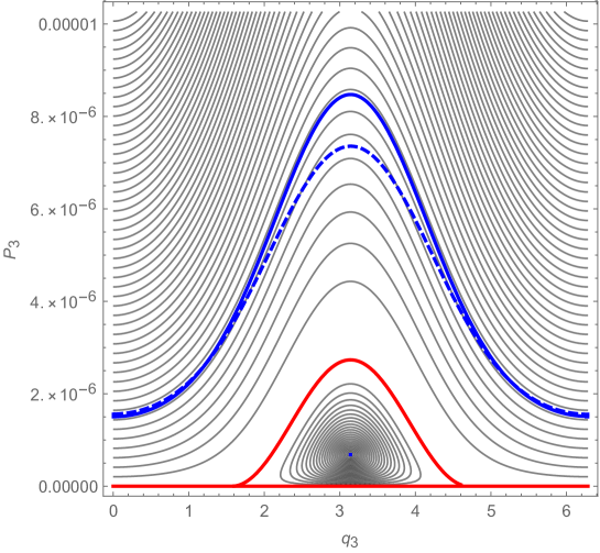
Figure 4. The Laplace resonance in the reduced phase-plane: the blue curves are the projections of the numerical integrations with the simplified model of Hamiltonian $H_{B}$ (continuous curve) and the 2nd-order model (dashed curve).

In this case the ensuing mean motions are

$$n_{1}=203.4847^{\circ}/day,\quad n_{2}=101.3746^{\circ}/day,\quad n_{3}=50.3196^{\circ}/day\ ,$$

which are reasonably close to the observed values (see Table 1), even if the resonant combinations

$$n_{1}-2n_{2}=n_{2}-2n_{3}=0.7355^{\circ}/day$$ (4.1)

turn out to be slightly different from the observed value $0.7395^{\circ}/day$ [Bro77]. However, we can see from Fig.5 that the Laplace angle has a quite small amplitude of libration: in the left panel we see the data as they are produced in the integration; in the right panel, the data are filtered with a time constant of 1000 days, so to allow a comparison with the fully-numerical solutions of Musotto et al. [MVMS02]. Also the libration period of about 2070 days seems to be almost correctly predicted.

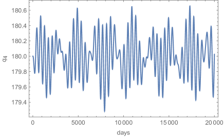
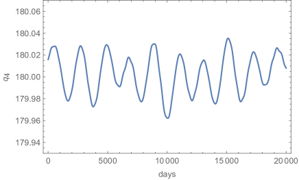
Figure 5. The Laplace angle: unfiltered data on the left; filtered data on the right. Days on the time-axis and angles in degrees.

In Fig.6 we report the corresponding results concerning the eccentricities. In the left panel, the three time evolutions of the eccentricities of Io, Europa and Ganymede are plotted as they are produced by the integrator. In the right panel, the data on the eccentricity of Io are filtered still with a time constant of 1000 days (the uprising curves are an artifact of the finite-time filtering operation).

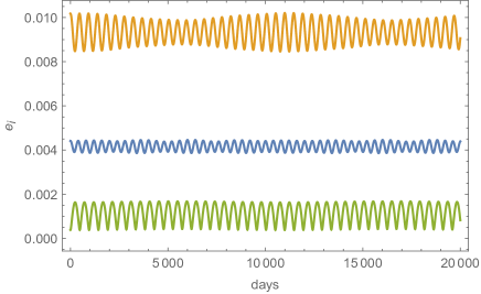
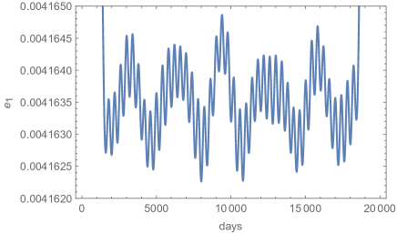
Figure 6. The eccentricities: in the left panel are plotted the eccentricities of Io (blue), Europa (orange) and Ganymede (green); in the right panel is plotted the filtered eccentricity of Io.

5. Conclusions

We have presented a simple model of the resonant interaction of the first three Galilean satellites of Jupiter. The back-bone of the Hamiltonian dynamical system associated with the model, based on the Keplerian and quadrupolar field of Jupiter and the first order self-interactions of the satellites, is captured by a 1-DOF normal form that permits to distinguish in a clear way the librational regime around the de Sitter equilibrium and the rotational one associated with the observed Laplace resonance.

We have investigated the uncertainties in the location of the de Sitter equilibrium, its sensitivity to higher-order perturbations and how close is the dynamics of the libration to the values which roughly correspond to the actually observed state. Looking at Fig.4, we can heuristically deduce that, starting with a value of $P_{3}$ which is chosen so to reproduce realistic semi-axes and eccentricities (notwithstanding the limitations of the model), the interval of initial values $q_{3}\in(135^{\circ},225^{\circ})$ corresponds to librating rather than rotating trajectories. This gives a measure of the difference between the solutions associated to the de Sitter and the Laplace states.

A possible observational test concerns the apsidal precession of Ganymede. In fact, from (3.4), since longitudes advance almost linearly in time, $\varpi_{3}$ should be modulated at the same 485-days period of the 2:1 commensurability, with an amplitude spanning $\sim 20^{\circ}$. We have checked this claim by using ephemerides (see the left panel of Fig.7) and verified with the outcome of the integration with our first-order model (see the right panel of Fig.7).

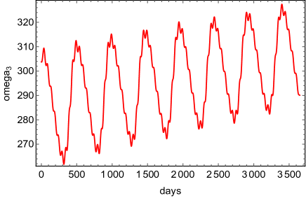
Figure 7. The apsidal precession of Ganymede: in the left panel is plotted the peri-jove as given by the ephemerides; in the right panel is plotted the outcome of the integration with the first-order model.

We conclude by mentioning that dissipative effects, like those due to tidal forces might induce an adiabatic variation of the parameters. The inclusion of such effects can lead to conclusions about a possible capture or escape from the exact resonance [HL83, Mal91]. This topic is certainly interesting and will be the object of a future study. It would also be interesting to apply the results of this work to test the nature of the Laplace resonance detected in extra-solar multi-planetary systems [BDH15, MCB16, Pap16], possibly extending the pioneering analysis made by Malhotra [Mal91] to the cases in which the 2:1 commensurabilities are not in the standard 1:1 ratio.

Appendix A Complete Hamiltonian in Henrard-Malhotra coordinates

The complete form of the Hamiltonian (2.22) including the Keplerian, the quadrupole field and the mutual interactions at first order in the eccentricities is:

$$H_{B}(P_{\alpha},q_{a}) = -\frac{m_{1}}{2(-P_{1}-P_{2}-P_{4}+P_{5})^{2}(1+\epsilon_{I})}$$

$$-\frac{m_{2}^{3}(1+\epsilon_{I})^{3}}{(2(P_{1}+P_{2})-P_{3}+3P_{4})^{2}(1+\epsilon_{E}+\epsilon_{I})}$$

$$-\frac{m_{3}^{3}(1+\epsilon_{E}+\epsilon_{I})^{3}}{(2P_{3}-2P_{4}-P_{5}+P_{6})^{2}(1+\epsilon_{E}+\epsilon_{G}+\epsilon_{I})}$$

$$-\frac{J_{2}R_{\jupiter}^{2}m_{1}^{7}(2P_{1}-P_{2}-P_{4}+P_{5})}{2(-P_{1}-P_{2}-P_{4}+P_{5})^{7}(1+\epsilon_{I})^{3}}$$

$$-\frac{J_{2}R_{\jupiter}^{2}m_{2}^{7}(3P_{2}+2(P_{1}+P_{2})-P_{3}+3P_{4})(1+\epsilon_{I})^{7}}{(2(P_{1}+P_{2})-P_{3}+3P_{4})^{7}(1+\epsilon_{E}+\epsilon_{I})^{3}}$$

$$-\frac{J_{2}R_{\jupiter}^{2}m_{3}^{7}(5P_{3}-2P_{4}-P_{5}+P_{6})(1+\epsilon_{E}+\epsilon_{I})^{7}}{(2P_{3}-2P_{4}-P_{5}+P_{6})^{7}(1+\epsilon_{E}+\epsilon_{G}+\epsilon_{I})^{3}}$$

$$-\frac{m_{1}m_{2}^{2}\epsilon_{E}(1+\epsilon_{I})^{2}}{(2(P_{1}+P_{2})-P_{3}+3P_{4})^{2}(1+\epsilon_{E}+\epsilon_{I})}\times$$

$$\left(b_{1}+\gamma_{11}\sqrt{\frac{2P_{1}}{-P_{1}-P_{2}-P_{4}+P_{5}}}\cos q_{1}+\gamma_{21}\sqrt{\frac{2P_{2}}{(2(P_{1}+P_{2})-P_{3}+3P_{4})}}\cos q_{2}\right)$$

$$-\frac{m_{2}m_{3}^{2}\epsilon_{G}(1+\epsilon_{E}+\epsilon_{I})^{2}}{(2P_{3}-2P_{4}-P_{5}+P_{6})^{2}(1+\epsilon_{G}+\epsilon_{E}+\epsilon_{I})}\times$$

$$\left(b_{2}+\gamma_{12}\sqrt{\frac{2P_{3}}{2P_{3}-2P_{4}-P_{5}+P_{6}}}\cos q_{3}+\gamma_{22}\sqrt{\frac{2P_{2}}{2(P_{1}+P_{2})-P_{3}+3P_{4}}}\cos(q_{2}-q_{4})\right)$$

$$-\frac{b_{3}m_{1}m_{3}^{2}\epsilon_{G}(1+\epsilon_{E}+\epsilon_{I})^{2}}{(2P_{3}-2P_{4}-P_{5}+P_{6})^{2}(1+\epsilon_{G}+\epsilon_{E}+\epsilon_{I})}\ .$$

In (A) the following definitions and abbreviations have been introduced:

$$\epsilon_{I} = \frac{m_{1}}{m_{0}}\ ,$$ (A.2)

$$\epsilon_{E} = \frac{m_{2}}{m_{0}}\ ,$$ (A.3)

$$\epsilon_{G} = \frac{m_{3}}{m_{0}}\ ,$$ (A.4)

$$b_{1} = {B_{0}}\left(\alpha_{12}\right)\ ,$$

$$b_{2} = {B_{0}}\left(\alpha_{23}\right)\ ,$$

$$b_{3} = {B_{0}}\left(\alpha_{13}\right)\ ,$$

$$\gamma_{11} = \gamma_{1}\left(\alpha_{12}\right)\ ,$$

$$\gamma_{12} = \gamma_{1}\left(\alpha_{23}\right)\ ,$$

$$\gamma_{21} = \gamma_{2}\left(\alpha_{12}\right)\ ,$$

$$\gamma_{22} = \gamma_{2}\left(\alpha_{23}\right)\ .$$

The mass ratios (A.2)–(A.4) are reported in Table 1, where the mass of Jupiter is taken as $m_{0}=1.898\times 10^{27}$ kg.

Appendix B Second-order model

The extended model contains the following terms [Mal91]: the satellite self-interactions at 2nd order in the eccentricities

$$H^{(2)}_{Sat}=-{{Gm_{1}m_{2}}\over a_{2}}R^{(12)}-{{Gm_{2}m_{3}}\over a_{3}}R^{(23)}-{{Gm_{1}m_{3}}\over a_{3}}R^{(13)}\ ,$$ (B.1)

with

$$R^{(12)} = \gamma_{0}\left(\alpha_{12}\right)(e_{1}^{2}+e_{2}^{2})+\gamma_{3}\left(\alpha_{12}\right)e_{1}^{2}\cos 2(2\lambda_{2}-\lambda_{1}-\varpi_{1})+\gamma_{4}\left(\alpha_{12}\right)e_{2}^{2}\cos 2(2\lambda_{2}-\lambda_{1}-\varpi_{2})\$$

$$+e_{1}e_{2}\left[\gamma_{5}\left(\alpha_{12}\right)\cos(4\lambda_{2}-2\lambda_{1}-\varpi_{2}-\varpi_{1})+\gamma_{6}\left(\alpha_{12}\right)\cos(\varpi_{2}-\varpi_{1})\right]\ ,$$

$$R^{(23)} = \gamma_{0}\left(\alpha_{23}\right)(e_{2}^{2}+e_{3}^{2})+\gamma_{3}\left(\alpha_{23}\right)e_{2}^{2}\cos 2(\lambda_{2}-2\lambda_{3}+\varpi_{2})+\gamma_{4}\left(\alpha_{23}\right)e_{3}^{2}\cos 2(\lambda_{2}-2\lambda_{3}+\varpi_{3})\$$

$$+e_{2}e_{3}\left[\gamma_{5}\left(\alpha_{23}\right)\cos(2\lambda_{2}-4\lambda_{3}+\varpi_{2}+\varpi_{3})+\gamma_{6}\left(\alpha_{23}\right)\cos(\varpi_{3}-\varpi_{2})\right]\ ,$$

$$R^{(13)} = \gamma_{0}\left(\alpha_{13}\right)(e_{1}^{2}+e_{3}^{2})+\gamma_{6}\left(\alpha_{13}\right)e_{1}e_{3}\cos(\varpi_{3}-\varpi_{1})\ ,$$

where $\gamma_{1}$ and $\gamma_{2}$ are defined in (2.4) and

$$\gamma_{0} = -{1\over 8}(2\alpha{d\over{d\alpha}}+\alpha^{2}{d^{2}\over{d\alpha^{2}}})b_{1/2}^{(0)}(\alpha)\ ,\qquad\qquad\gamma_{3}=-{1\over 8}(44+14\alpha{d\over{d\alpha}}+\alpha^{2}{d^{2}\over{d\alpha^{2}}})b_{1/2}^{(4)}(\alpha)\ ,$$

$$\gamma_{4} = -{1\over 8}(38+14\alpha{d\over{d\alpha}}+\alpha^{2}{d^{2}\over{d\alpha^{2}}})b_{1/2}^{(2)}(\alpha)\ ,\qquad\gamma_{5}={1\over 4}(42+14\alpha{d\over{d\alpha}}+\alpha^{2}{d^{2}\over{d\alpha^{2}}})b_{1/2}^{(3)}(\alpha)\ ,$$

$$\gamma_{6} = -{1\over 4}(2-2\alpha{d\over{d\alpha}}-\alpha^{2}{d^{2}\over{d\alpha^{2}}})b_{1/2}^{(1)}(\alpha)\ ,$$

the secular influence of Callisto and the Sun

$$H_{p} = -{{Gm_{1}m_{p}}\over a_{p}}\left\{{1\over 2}b_{1/2}^{(0)}\left({a_{1}\over a_{p}}\right)-1+{1\over 8}{a_{1}\over a_{p}}b_{3/2}^{(1)}\left({a_{1}\over a_{p}}\right)(e_{1}^{2}+e_{p}^{2})\right\}$$

$$- {{Gm_{2}m_{p}}\over a_{p}}\left\{{1\over 2}b_{1/2}^{(0)}\left({a_{2}\over a_{p}}\right)-1+{1\over 8}{a_{2}\over a_{p}}b_{3/2}^{(1)}\left({a_{2}\over a_{p}}\right)(e_{2}^{2}+e_{p}^{2})\right\}$$

$$- {{Gm_{3}m_{p}}\over a_{p}}\left\{{1\over 2}b_{1/2}^{(0)}\left({a_{3}\over a_{p}}\right)-1+{1\over 8}{a_{3}\over a_{p}}b_{3/2}^{(1)}\left({a_{3}\over a_{p}}\right)(e_{3}^{2}+e_{p}^{2})\right\}\ ,$$

where the subindex $p$ denotes either Callisto or the Sun, while $m_{p}$, $a_{p}$, $e_{p}$ are, respectively, the corresponding mass, semimajor axis, eccentricity and the octupolar terms of Jupiter gravitational field

$$H_{J_{4}}={{3Gm_{0}J_{4}R_{\jupiter}^{4}}\over{8}}\ \left[{m_{1}\over a_{1}^{4}}\left(1+{5\over 2}e_{1}^{2}\right)+{m_{1}+m_{2}\over a_{2}^{4}}\left(1+{5\over 2}e_{2}^{2}\right)+{m_{1}+m_{2}+m_{3}\over a_{3}^{4}}\left(1+{5\over 2}e_{3}^{2}\right)\right]\ ,$$

where $J_{4}=-5.87\times 10^{-4}$.

References

- [BDH15] K. Batygin, K. M. Deck, and M. J. Holman. Dynamical Evolution of Multi-resonant Systems: the Case of GJ876. Astronomical Journal, 149:167–182, 2015.
- [BH16] H. W. Broer and H. Hanßmann. On Jupiter and his Galilean satellites: Librations of de Sitter’s periodic motions. Indagationes Mathematicae, 27:1305–1336, 2016.
- [Bro77] B. Brown. The long period behavior of the orbits of the Galilean satellites of Jupiter. Celestial Mechanics, 16:229–259, 1977.
- [BZ17] H. W. Broer and L. Zhao. De Sitter’s theory of Galilean satellites. Cel. Mech. Dyn. Astr., 127:95–119, 2017.
- [dS31] W. de Sitter. Jupiter’s Galilean satellites. Monthly Notices of the Royal Astronomical Society, 91:706–738, 1931.
- [Eft11] C. Efthymiopoulos. Canonical perturbation theory; stability and diffusion in Hamiltonian systems: applications in dynamical astronomy. Third La Plata International School on Astronomy and Geophysics, Edited by P.M. Cincotta, C.M. Giordano, and C. Efthymiopoulos, Asociación Argentina de Astronomia Workshop Series, Vol. 3, 3–146, 2011.
- [FM79] S. Ferraz-Mello. Dynamics of the Galilean Satellites: An Introductory Treatise. Instituto Astronomico e Geofi sico, Universidade de Sāo Paulo, 1979.
- [Gio02] A. Giorgilli. Notes on Exponential Stability of Hamiltonian Systems. Centro di Ricerca Matematica E. De Giorgi, Pisa, 2002.
- [Hen84] J. Henrard. Libration of Laplace’s argument in the Galilean satellites theory. Celestial Mechanics, 34:255–262, 1984.
- [HL83] J. Henrard and A. Lemaitre. A second fundamental model for resonance. Celestial Mechanics, 30:197–218, 1983.
- [HM81] J.D. Hadjidemetriou and M. Michalodimitrakis. Periodic Planetary-type Orbits of the General 4-Body Problem with an Application to the Satellites of Jupiter. Astronomy and Astrophysics, 93:204–211, 1981.
- [Kam70] A.A. Kamel. Perturbation method in the theory of nonlinear oscillations. Celestial Mechanics, 3:90–106, 1970.
- [LDV04] V. Lainey, L. Duriez, and A. Vienne. New accurate ephemerides for the Galilean satellites of Jupiter (I). Astronomy and Astrophysics, 420:1171–1183, 2004.
- [Mal91] R. Malhotra. Tidal Origin of the Laplace Resonance and the Resurfacing of Ganymede. Icarus, 94:399–412, 1991.
- [MCB16] J. G. Martí, P. M. Cincotta, and C. Beaugé. Chaotic Diffusion in the Gliese-876 Planetary System. Monthly Notices of the Royal Astronomical Society, 460:1094–1105, 2016.
- [MD99] C. D. Murray and S. F. Dermott. Solar system dynamics. Cambridge, UK: Cambridge University Press, 1999.
- [MVMS02] S. Musotto, F. Varadi, W. Moore, and G. Schubert. Numerical Simulations of the Orbits of the Galilean Satellites. Icarus, 159:500–504, 2002.
- [Pap16] J. C. B. Papaloizou. Consequences of tidal interaction between disks and orbiting protoplanets for the evolution of multi-planet systems with architecture resembling that of Kepler 444. Celestial Mechanics and Dynamical Astronomy, 126:157–187, November 2016.
- [Poi99] H. Poincaré. Les méthodes nouvelles de la méchanique céleste. 1899.
- [SM97] A.P. Showman and R. Malhotra. Tidal Evolution into the Laplace Resonance and the Resurfacing of Ganymede. Icarus, 127:93–111, 1997.
- [YP81] C.F. Yoder and S.J. Peale. The Tides of Io. Icarus, 47:1–35, 1981.