Constructive Matrix Theory
for Higher Order Interaction

Abstract

This paper provides an extension of the constructive loop vertex expansion to stable matrix models with interactions of arbitrarily high order. We introduce a new representation for such models, then perform a forest expansion on this representation. It allows us to prove that the perturbation series of the free energy for such models is analytic in a domain uniform in the size $N$ of the matrix.

LPT-20XX-xx

MSC: 81T08, Pacs numbers: 11.10.Cd, 11.10.Ef
Key words: Matrix Models, constructive field theory, Loop vertex expansion.

I Introduction

The loop vertex expansion (LVE) was introduced in [1] to provide a constructive method for quartic matrix models uniform in the size of the matrix. In its initial version it combines an intermediate field representation with replica fields and a forest formula [2, 3] to express the free energy of the theory in terms of a convergent sum over trees. This loop vertex expansion in contrast with traditional constructive methods is not based on cluster expansions nor involves small/large field conditions.

• Like Feynman’s perturbative expansion, the LVE allows to compute connected quantities at a glance: the partition function of the theory is expressed by a sum over forests, and its logarithm is exactly the same sum but restricted to connected forests, i.e. trees. This is simply because the amplitudes factorize over the connected components of the forest,

• the functional integrands associated to each forest or tree are absolutely and uniformly convergent for any value of the fields,

• the convergence of the LVE implies Borel summability of the usual perturbation series and the LVE directly computes the Borel sum,

• the LVE is in fact conceptually an explicit repacking of infinitely many subsets of pieces of Feynman amplitudes so that the packets provide a convergent rather than divergent expansion [4].

• in the case of combinatorial field theories of the matrix and tensor type [5, 6], suitably rescaled to have a non-trivial $N\to\infty$ limit [7, 8, 9, 10], the Borel summability obtained in this way is uniform in the size $N$ of the model [1, 11, 12, 13].

The LVE method can be developed for ordinary field theories with cutoffs [14]. A multiscale version (MLVE) [16] can include renormalization [17, 18, 19, 20, 21] . This MLVE is especially adapted to resum the renormalized series of non-local field theories of the matrix or tensorial type. For ordinary local field theories, and in contrast with the more traditional constructive methods such as cluster and Mayer expansions, it is still until now less efficient in providing the spatial decay of truncated functions. See however [14] and [15].

There was until recently a big limitation of the method: it did apply only to quartic interactions. Progress to generalize the LVE to interactions of higher order has been slow. It is possible to generalize the intermediate field representation to interactions of order higher than 4 [22, 23, 24], using several intermediate fields. However these representations all imply oscillating Gaussian integrals and lead for matrix or tensor models to analyticity domains for the free energy which are not uniform in the size $N$ of the matrix or tensor [23, 24].

In [25] a new representation, called loop vertex representation (hereafter LVR), was introduced in the simple case of scalar monomial interactions of arbitrarily high even order. It does not suffer from the previous defects and it uses the initial fields of the model rather than intermediate fields. It was found through selective Gaussian integration of one particular field per vertex, hence giving rise to a new kind of “single loop” vertex similar to those found in the Gallavotti quantum field theoretic version of classical mechanics [26] or in the quantum field theory formulation of the Jacobian conjecture [27, 28], see also [29] for an algebraic version of this formalism. It was quickly noticed that this LVR representation is in fact a reparametrization of the functional integrand into a Gaussian one. The single loop vertices form the natural expansion of the Jacobian of the transformation, which is a determinant. This is the deep reason for which the LVE applied to this new representation then works. Indeed a determinant has slow “logarithmic” growth at large field. In particular its partial derivatives are typically bounded. The LVE could never converge for the initial Bosonic interactions because it has unbounded derivatives at large field.

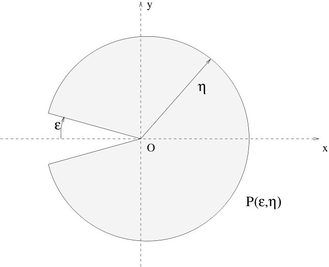
Figure 1: A pacman domain

In this paper we apply the idea of reparametrization invariance to matrix models and essentially extend the results of [11] to monomial interactions of arbitrarily high even order. Our main result, the Theorem III.1 states that the free energy of such models is analytic for $\lambda$ in an open “pacman domain” (see Figure 1)

$$P(\epsilon,\eta):=\{0<|\lambda|<\eta,|\arg\lambda|<\pi-\epsilon\},$$ (I-1)

with $\epsilon$ and $\eta$ positive and small numbers independent of the size $N$ of the matrix. Extension of this theorem to cumulants and a constructive version of the $1/N$ expansion are also consequences of the method left to the reader. We intend also to explore links with the topological recursion approach to random matrices [30].

An unexpected difficulty of this paper compared to [1], [25] or [11] is to deal with the non-factorization of the two sides of the ribbon loop in a vertex of the loop vertex representation. Fortunately this difficulty can be solved by using Cauchy holomorphic matrix calculus, which allows to factorize the matrix dependence on the two sides of the ribbon, see Lemma II.3 below. The price to pay is that one has to prove convergence of these contour integrals and this requires a bit of convex analysis.

The plan of our paper goes as follows. In section II we introduce the LVR representation and its factorization through holomorphic calculus. In section III we perform the LVE on this representation. In Section IV we establish the functional integral and contour bounds, completing the proof of Theorem III.1. Four appendices gather some additional aspects: the first one is devoted to an alternative derivation of the LVR, the second one to an integral representation of the Fuss-Catalan function that we need for the third one, devoted to the justification of the LVR beyond perturbation theory and the last appendix is devoted to its relationship to the ordinary perturbation theory.

II Effective action

Consider a complex matrix model with stable interaction of order $2p$, where $p\geq 2$ is an integer which is fixed through all this paper. The model has partition function

$$Z(\lambda,N) := \int\,dMdM^{\dagger}\,e^{-NS(M,M^{\dagger})},$$ (II-2)

$$S(M,M^{\dagger}) := {\rm Tr}\{MM^{\dagger}+\lambda(MM^{\dagger})^{p}\}.$$ (II-3)

$M$ is a random complex square matrix of size $N$ and the stable case corresponds to a positive coupling constant $\lambda$. The goal is to compute the “free energy”

$$F(\lambda,N):=\frac{1}{N^{2}}\log Z[\lambda,N]$$ (II-4)

for $\lambda$ in a domain independent of $N$. The case of a rectangular $N_{l}\times N_{r}$ matrix is also important, as it allows to interpolate between vectors and matrices, and to better distinguish rows and columns. We can introduce the Hilbert spaces ${\cal{H}}_{l}$ with $\dim{\cal{H}}_{l}=N_{l}$ and ${\cal{H}}_{r}$ with $\dim{\cal{H}}_{r}=N_{r}$. Remark that the two matrices $MM^{\dagger}$ and $M^{\dagger}M$ are distinct, the first one being $N_{l}$ by $N_{l}$ and the second $N_{r}$ by $N_{r}$, but crucially for what follows they have the same trace, so all our computations will be done involving only one of them, say $MM^{\dagger}$. In tensor products we may distinguish left and right factors; for instance $A\otimes_{lr}B$ means an element of ${\cal{H}}_{lr}:={\cal{H}}_{l}\otimes{\cal{H}}_{r}$, ${\bf{1}}_{lr}$ the identity in ${\cal{H}}_{lr}$ and so on. For simplicity and without loss of generality we can assume $N_{l}\leq N_{r}$. Then, the partition function in the rectangular case is

$$Z(\lambda,N_{l},N_{r}) := \int\,dMdM^{\dagger}\,e^{-N_{r}S(M,M^{\dagger})},$$ (II-5)

$$S(M,M^{\dagger}) := {\rm Tr}_{l}\{MM^{\dagger}+\lambda(MM^{\dagger})^{p}\}.$$ (II-6)

and the quantity of interest is

$$F(\lambda,N_{l},N_{r}):=\frac{1}{N_{l}N_{r}}\log Z(\lambda,N_{l},N_{r}).$$ (II-7)

Of course there are similar formulas using right traces ${\rm Tr}_{r}$. Also sources can be introduced to compute cumulants etc…

The standard perturbative approach to models of type (II-2) or (II-5) expands the exponential of the interaction into a Taylor series. However, polynomial interactions lead to divergent perturbative expansions. To avoid this problem, we folllow the strategy of [25] and first rewrite $Z[\lambda,N_{l},N_{r}]$ in another integral representation, called the loop vertex representation (LVR), in which the interaction grows only logarithmically at large fields. One of the key elements of the LVR construction is the Fuss-Catalan function $T_{p}$ [32] defined to be the solution analytic at the origin of the algebraic equation

$$zT_{p}^{p}(z)-T_{p}(z)+1=0\,.$$ (II-8)

For any square matrix $X$ we also define the matrix-valued function

$$A(\lambda,X) := XT_{p}(-\lambda X^{p-1})\,$$ (II-9)

so that from (II-8)

$$X=A(\lambda,X)+\lambda A^{p}(\lambda,X)\,.$$ (II-10)

We often write simply $A(X)$ for $A(\lambda,X)$ when no confusion is possible. Finally we define an $N_{l}$ by $N_{l}$ square matrix $X_{l}$ and an $N_{r}$ by $N_{r}$ square matrix $X_{r}$ through

$$X_{l} := MM^{\dagger},\quad X_{r}:=M^{\dagger}M.$$ (II-11)

The loop vertex representation is then given by

Theorem II.1.

In the sense of formal power series in $\lambda$

$$Z(\lambda,N_{l},N_{r}) = \int\,dMdM^{\dagger}\,\exp\{-N_{r}{\rm Tr}_{l}X_{l}+{\cal{S}}(X_{l},X_{r})\}$$

where ${\cal{S}}$, the loop vertex action is

$${\cal{S}}(X_{l},X_{r}) = -{\rm Tr}_{lr}\log\Big{[}{\bf{1}}_{lr}+\lambda\sum_{k=0}^{p-1}A^{k}(X_{l})\otimes_{lr}A^{p-1-k}(X_{r})\Big{]}.$$

In (LABEL:ZAgood) the $N_{l}$ by $N_{l}$ matrix $A^{k}(X_{l})$ acts on the left index of ${\cal{H}}_{lr}$ and the $N_{r}$ by $N_{r}$ matrix $A^{p-1-k}(X_{r})$ acts on the right index of ${\cal{H}}_{lr}$.

Proof.

Remark first that this formula exactly coincides with equations (II.12) and (II.16) of [25] in the scalar case $N_{l}=N_{r}=1$. We work first at the level of formal power series in order not to worry about convergence. However Theorem II.1 holds beyond formal power series as proved in Appendix C.

Since (LABEL:ZAgood) is crucial for the rest of the paper we propose two different proofs. The first one, below, relies on a change of variables on $M$ and the computation of a Jacobian. A second perhaps more concrete proof relies as in [25] on Gaussian integration and will be given in Appendix A.

We perform a change of variables $M\to P$ where $P$ is again an $N_{l}$ by $N_{r}$ rectangular matrix. We write

$$Y_{l} := PP^{\dagger},\quad Y_{r}:=P^{\dagger}P$$ (II-13)

and define $P(M)$ (up to unitary conjugation) through the implicit function formal power series equation

$$X_{l} := A(Y_{l}),\quad X_{r}:=A(Y_{r}).$$ (II-14)

Thanks to (II-10), the action transforms to

$$S(M,M^{\dagger})={\rm Tr}_{l}(X_{l}+\lambda X_{l}^{p})={\rm Tr}_{l}[A(Y_{l})+\lambda A^{p}(Y_{l})]={\rm Tr}_{l}Y_{l}.$$ (II-15)

hence it becomes the ordinary Gaussian measure on $P,P^{\dagger}$. The new interaction lies therefore entirely in the Jacobian of the $M\to P$ transformation. The transformation (II-13), (II-14) can be written more explicitly as

$$M := PP^{\dagger}T_{p}(-\lambda(PP^{\dagger})^{p-1})(P^{\dagger})^{-1}=A(PP^{\dagger})(P^{\dagger})^{-1}\,,$$

$$M^{\dagger} := P^{\dagger}\,.$$ (II-16)

Then, the corresponding Jacobian can be computed as

$$\Big{|}\det\begin{bmatrix}\frac{dM}{dP}&\frac{dM}{dP^{\dagger}}\\ \frac{dM^{\dagger}}{dP}&\frac{dM^{\dagger}}{dP^{\dagger}}\end{bmatrix}\Big{|} = \Big{|}\det\begin{bmatrix}\frac{dM}{dX_{l}}\frac{dX_{l}}{dP}&\frac{dM}{dP^{\dagger}}\\ \mathbf{0}&\mathbf{1}\end{bmatrix}\Big{|}$$

$$= \Big{|}\det\frac{A(Y_{l})\otimes_{lr}\mathbf{1}-\mathbf{1}\otimes_{lr}A(Y_{r})}{Y_{l}\otimes_{lr}\mathbf{1}-\mathbf{1}\otimes_{lr}Y_{r}}\Big{|}$$

$$= \exp\Big{\{}{\rm Tr}_{lr}\log\Big{[}\frac{A(Y_{l})\otimes_{lr}\mathbf{1}-\mathbf{1}\otimes_{lr}A(Y_{r})}{Y_{l}\otimes_{lr}\mathbf{1}-\mathbf{1}\otimes_{lr}Y_{r}}\Big{]}\Big{\}}\,,$$

where the symbolic matrix differentiation rule valid for analytic functions $f$ of a matrix

$$\frac{\delta f(X)}{\delta X}=\frac{f(X)\otimes\mathbf{1}-\mathbf{1}\otimes f(X)}{X\otimes\mathbf{1}-\mathbf{1}\otimes X}\,,$$ (II-18)

was used and the trace and tensor product acts on the Hilbert space ${\cal{H}}_{l}\otimes{\cal{H}}_{r}$. The absolute value in (II) can be omitted through a perturbative regularity check.

Since it is a dummy variable, renaming $P$ as $M$ , hence $Y$ as $X$, yields

$$Z(\lambda,N_{l},N_{r}) = \int\,dMdM^{\dagger}\,\exp\{-N_{r}{\rm Tr}_{l}X_{l}+{\cal{S}}(X_{l},X_{r})\},$$ (II-19)

$${\cal{S}}(X_{l},X_{r}) = {\rm Tr}_{lr}\log\Big{[}\frac{A(X_{l})\otimes_{lr}\mathbf{1}-\mathbf{1}\otimes_{lr}A(X_{r})}{X_{l}\otimes_{lr}\mathbf{1}-\mathbf{1}\otimes_{lr}X_{r}}\Big{]}\,.$$ (II-20)

Taking into account the functional equation (II-10) one can rewrite the loop vertex action as

$${\cal{S}} = {\rm Tr}_{lr}\log\Big{[}\frac{(A(X_{l})+\lambda A^{p}(X_{l}))\otimes_{lr}\mathbf{1}-\mathbf{1}\otimes_{lr}(A(X_{r})+\lambda A^{p}(X_{r}))}{A(X_{l})\otimes_{lr}\mathbf{1}-\mathbf{1}\otimes_{lr}A(X_{r})}\Big{]}^{-1}$$ (II-21)

$$= -{\rm Tr}_{lr}\log\Big{[}{\bf{1}}_{lr}+\lambda\frac{A^{p}(X_{l})\otimes_{lr}\mathbf{1}-\mathbf{1}\otimes_{lr}A^{p}(X_{r})}{A(X_{l})\otimes_{lr}\mathbf{1}-\mathbf{1}\otimes_{lr}A(X_{r})}\Big{]}$$

$$= -{\rm Tr}_{lr}\log\Big{[}{\bf{1}}_{lr}+\lambda\sum_{k=0}^{p-1}A^{k}(X_{l})\otimes_{lr}A^{p-1-k}(X_{r})\Big{]}\,.$$

∎

Let us now rewrite ${\cal{S}}$ in terms of $X_{l}$ alone. Developing the logarithm in powers and taking the (factorized) tensor trace leads to

$${\cal{S}}(X_{l},X_{r})=\sum_{n=1}^{\infty}\frac{(-\lambda)^{n}}{n}\sum_{k_{1}=0}^{p-1}\cdots\sum_{k_{n}=0}^{p-1}[{\rm Tr}_{l}A^{\sum k_{i}}(X_{l})][{\rm Tr}_{r}A^{\sum(p-k_{i}-1)}(X_{r})].$$ (II-22)

Since $A(x)=\sum_{n=1}^{\infty}a_{n}x^{n}$ and since ${\rm Tr}_{l}X_{l}^{q}={\rm Tr}_{r}X_{r}^{q}$ for any $q>0$ we can rewrite everything in this sum in terms of $X_{l}$ alone hence as a tensor trace on ${\cal{H}}_{l}\otimes{\cal{H}}_{l}$. We have however to be careful to the fact that ${\rm Tr}_{l}1_{l}=N_{l}\neq{\rm Tr}_{r}1_{r}=N_{r}$. A moment of attention therefore reveals that the loop vertex action ${\cal{S}}$ is the sum of a “square matrix” piece and a “vector piece” (without any tensor product)

$${\cal{S}}(X_{l}) = {\cal{S}}^{{\text{M}at}}(X_{l})+{\cal{S}}^{{\text{V}ec}}(X_{l}),$$ (II-23)

$${\cal{S}}^{{\text{M}at}}(X_{l}) = -{\rm Tr}_{ll}\log\big{[}{\bf{1}}_{ll}+\lambda\sum_{k=0}^{p-1}A^{k}(X_{l})\otimes_{ll}A^{p-1-k}(X_{l})\big{]},$$ (II-24)

$${\cal{S}}^{{\text{V}ec}}(X_{l}) = -(N_{r}-N_{l}){\rm Tr}_{l}\log[{\bf{1}}_{l}+\lambda A^{p-1}(X_{l})].$$ (II-25)

For simplicity from now on we limit ourselves to the square case $N_{l}=N_{r}=N$, but we emphasize that our main result, namely uniform analyticity in $N$, extends to the rectangular case, uniformity being in the largest dimension $N_{r}$ in that case. The treatment of the additional vector piece ${\cal{S}}^{Vec}$ in (II-23) is indeed almost trivial compared to the matrix piece, and the corresponding details are left to the reader.

From now on since the right space has disappeared we simply write $X$ instead of $X_{l}$, ${\bf{1}}_{\otimes}$ instead of ${\bf{1}}_{ll}$ etc… Our starting point rewrites in these simpler notations

$$Z(\lambda,N) = \int\,dMdM^{\dagger}\,\exp\{-N{\rm Tr}\,X+{\cal{S}}\},$$ (II-26)

$${\cal{S}}(\lambda,X) = -{\rm Tr}_{\otimes}\log\Big{[}{\bf{1}}_{\otimes}+\lambda\sum_{k=0}^{p-1}A^{k}(X)\otimes A^{p-1-k}(X)\Big{]}.$$ (II-27)

Defining $\Sigma(\lambda,X):=\sum_{k=0}^{p-1}A^{k}(X)\otimes A^{p-1-k}(X)$, a useful lemma is

Lemma II.1.

$$\frac{\partial A}{\partial X}=\big{[}{\bf{1}}_{\otimes}+\lambda\Sigma(\lambda,X)\big{]}^{-1}.$$ (II-28)

Proof  From the algebraic rule (II-18) and the functional equation (II-10)

$$\frac{\partial A}{\partial X} = \Big{[}\frac{(A(X)+\lambda A^{p}(X))\otimes 1-1\otimes(A(X)+\lambda A^{p}(X))}{A(X)\otimes 1-1\otimes A(X)}\Big{]}^{-1}$$

$$= \Big{[}{\bf{1}}_{\otimes}+\lambda\frac{A^{p}(X)\otimes 1-1\otimes A^{p}(X)}{A(X)\otimes 1-1\otimes A(X)}\Big{]}^{-1}$$

$$= \Big{[}{\bf{1}}_{\otimes}+\lambda\sum_{k=0}^{p-1}A^{k}(X)\otimes A^{p-1-k}(X)\Big{]}^{-1}=\big{[}{\bf{1}}_{\otimes}+\lambda\Sigma(\lambda,X)\big{]}^{-1}.$$

∎

II.1 Factorization through Holomorphic Calculus

We shall now establish another equivalent formula for ${\cal{S}}$ factorized over left and right pieces. Given a holomorphic function $f$ on a domain containing the spectrum of a square matrix $X$, Cauchy’s integral formula yields a convenient expression for $f(X)$,

$$f(X)=\oint_{\Gamma}dw\frac{f(w)}{w-X},$$ (II-30)

provided the contour $\Gamma$ encloses the full spectrum of $X$.

We work with Hermitian matrices such as $X$ which have positive spectrum. Let us introduce a bit of notation for the contours that we shall use.

Let’s assume we have two radii $0<r<R<+\infty$ and an angle $\psi\in]0,\frac{\pi}{2}[$. The finite keyhole contour $\Gamma^{f}_{r,R,\psi}$ is defined as the (counterclockwise) contour in the complex plane made of the two segments $H^{\pm}_{r,R,\psi}$ joining the points $re^{\pm i\psi}$ and $Re^{\pm i\psi}$, plus two arcs of circle namely $C_{R,\psi}$ corresponding to radius $R$ and arguments in $[-\psi,\psi]$ and $\bar{C}_{r,\psi}$ corresponding to radius $r$ and arguments out of $]-\psi,\psi[$, see Figure 2.

Figure 2: A finite keyhole contour $\Gamma^{f}_{r,R,\psi}$ encircling a segment on the real positive $Ox$ axis, shown in boldface, which includes the spectrum of $X$.

Since the matrix $X$ is positive Hermitian, the condition for holomorphic calculus is fulfilled as soon as $R>\|X\|$. For the moment we always assume this condition to be fulfilled.

We also define the infinite keyhole contour $\Gamma^{\infty}_{r,\psi}$ which is the $R\to\infty$ limit of $\Gamma^{f}_{r,R,\psi}$. Of course we shall use them only when the associated infinite contour integral is absolutely convergent.

In the following we call scalar counterparts of matrix functions by the same, but small (not capital) letters. Thus, the function $A(\lambda,X)$ is represented by the Cauchy’s formula of $a(\lambda,u)$. We may omit the $r,R,\psi$ indices when the context is clear.

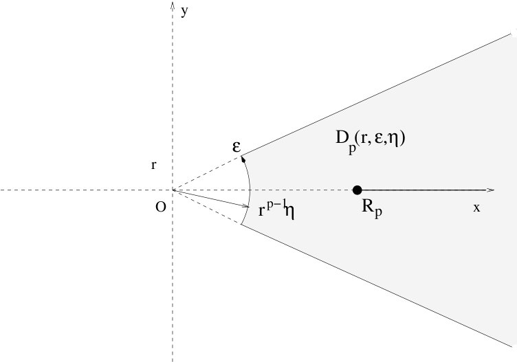
Figure 3: The cut-sector $D_{p}(r,\epsilon,\eta)$ containing the Fuss-Catalan cut starting at $R_{p}$ (shown in boldface).

Lemma II.2.

Suppose $\lambda\in P(\epsilon,\eta)$. For sufficiently small $r$ and $\psi$ the function $a^{k}(\lambda,u)$ is analytic in $u$ in an open neighborhood of the contour $\Gamma^{f}_{r,R,\psi}$ for any integer $k\in[0,p-1]$.

Proof  Write $\lambda=\rho e^{i\theta}$ with $\rho<\eta$, $|\theta|<\pi-\epsilon$, and remember $\Gamma^{f}_{r,R,\psi}=H^{-}_{r,R,\psi}\cup C_{R,\psi}\cup H^{+}_{r,R,\psi}\cup\bar{C}_{r,\psi}$. For $u\in H^{-}_{r,R,\psi}\cup C_{R,\psi}\cup H^{+}_{r,R,\psi}$ we have $|\arg u\,|\leq\psi$ hence $|\arg u^{p-1}|\leq(p-1)\psi$, hence if we choose $\psi<\frac{1}{2(p-1)}\epsilon$, then $\arg(-\lambda u^{p-1})$ is out of the interval $[-\frac{\epsilon}{2},\frac{\epsilon}{2}]$. Finally if $u\in\bar{C}_{r,\psi}$ then $|-\lambda u^{p-1}|\leq r^{p-1}\eta$. In conclusion for $u\in\Gamma^{f}_{r,R,\psi}$, $z=-\lambda u^{p-1}$ stays completely out of the cut-sector

$$D_{p}(r,\epsilon,\eta)=\{z\in{\mathbb{C}},|z|\geq r^{p-1}\eta,|\arg z|\leq\frac{\epsilon}{2}\}.$$ (II-31)

Let us assume from now on that $r^{p-1}\eta<R_{p}:=\frac{(p-1)^{p-1}}{p^{p}}$. Then this cut sector $D_{p}(r,\epsilon,\eta)$ fully contains the cut of the Fuss Catalan function $T_{p}$ which is $[R_{p},\infty)$ [25, 32]. It follows that $T_{p}(-\lambda u^{p-1})$, hence also $a^{k}(\lambda,u)$ for any integer $k\in[0,p-1]$, are analytic in $u$ in a neighborhood of the keyhole contour $\Gamma^{f}_{r,R,\psi}$ and that the contour integrals (II-32)-(II-33) are well defined. ∎

We can therefore write

$$A(X)=\oint_{\Gamma}du\;a(\lambda,u)\,\frac{1}{u-X}$$ (II-32)

where $a(\lambda,z)=zT_{p}(-\lambda z^{p-1})$ (see (II-9)) and the contour $\Gamma$ is a finite keyhole contour enclosing all the spectrum of $X$. The matrix derivative acting on a resolvent being easy to compute using (II-18) we obtain

$$\frac{\partial A}{\partial X}=\oint_{\Gamma}du\;a(\lambda,u)\frac{1}{u-X}\otimes\frac{1}{u-X}.$$ (II-33)

Resolvent factors such as $\frac{1}{u-X}$ are obviously non-singular on keyhole contours such as $\Gamma$ as they have all singularities inside by our choice of $R>\|X\|$. For safety of some formulas below and in the next sections we shall even always assume $R\geq 1+\|X\|$ so that we never even come close to a singularity of $\frac{1}{u-X}$. But the reader could worry about the $a$ functions in (II-32)-(II-33), in particular when $\lambda$ is complex in the pacman domain of (I-1). This is taken care of by our next Lemma.

Combining (II-27), (II-28) and (II-33) we get, for $\Gamma_{0}$ a finite keyhole contour enclosing the spectrum of $X$

$$\partial_{\lambda}{\cal{S}}=-\sum_{k=0}^{p-1}\oint_{\Gamma_{0}}du\;a(\lambda,u){\rm Tr}_{\otimes}\partial_{\lambda}\big{[}\frac{A^{k}(\lambda,X)}{u-X}\otimes\frac{A^{p-k-1}(\lambda,X)}{u-X}\big{]}.$$ (II-34)

Now we reapply the holomorphic calculus, but in different ways depending on the term chosen in the sum over $k$.

Figure 4: A keyhole contour $\Gamma_{1}$ encircling a keyhole contour $\Gamma_{0}$. The spectrum of $X$ lies on a real axis positive segment like the one shown in boldface.

• For $k=0$, we apply the holomorphic calculus to the right $\frac{A^{p-1}(\lambda,X)}{u-X}$ factor, with a contour $\Gamma_{2}$ surrounding $\Gamma_{0}$ for a new variable called $v_{2}$, and we rename $u$ and $\Gamma_{0}$ as $v_{1}$ and $\Gamma_{1}$ (see Figure 4),

• For $k=p-1$, we apply the holomorphic calculus to the left $\frac{A^{p-1}(\lambda,X)}{u-X}$ factor, with a contour $\Gamma_{2}$ surrounding $\Gamma_{0}$ for a new variable called $v_{2}$, and we rename $u$ and $\Gamma_{0}$ as $v_{1}$ and $\Gamma_{1}$; we obtain a contribution identical to the previous case.

• In all other cases, hence for $1\leq k\leq p-2$ we apply the holomorphic calculus both to left and right factors in the tensor product, with two variables $v_{1}$ and $v_{2}$ and two equal contours $\Gamma_{1}$ and $\Gamma_{2}$ enclosing enclose the contour $\Gamma_{0}$ .

In this way defining the “loop resolvent”

$${\cal{R}}(v_{1},v_{2},X):=\Big{[}{\rm Tr}\frac{1}{v_{1}-X}\Big{]}\Big{[}{\rm Tr}\frac{1}{v_{2}-X}\Big{]}$$ (II-35)

we obtain

$$\frac{\partial{\cal{S}}}{\partial\lambda} = -\oint_{\Gamma_{1}}dv_{1}\oint_{\Gamma_{2}}dv_{2}\Big{\{}\oint_{\Gamma_{0}}du\;a(\lambda,u)\sum_{k=1}^{p-2}\frac{\partial_{\lambda}[\lambda a^{k}(\lambda,v_{1})a^{p-k-1}(\lambda,v_{2})]}{(v_{1}-u)(v_{2}-u)}\,$$ (II-36)

$$\qquad+\;2a(\lambda,v_{1})\frac{\partial_{\lambda}\big{[}\lambda a^{p-1}(\lambda,v_{2})\big{]}}{v_{1}-v_{2}}\Big{\}}{\cal{R}}(v_{1},v_{2},X).$$

Therefore defining the weights

$$\phi(\lambda,u,v_{1},v_{2}):=-\sum_{k=1}^{p-2}\frac{1}{v_{1}-u}\frac{1}{v_{2}-u}a(\lambda,u)\partial_{\lambda}\big{[}\lambda a^{k}(\lambda,v_{1})a^{p-k-1}(\lambda,v_{2})\big{]}$$ (II-37)

$$\psi(\lambda,v_{1},v_{2}):=-\frac{2}{v_{1}-v_{2}}a(\lambda,v_{1})\partial_{\lambda}\big{[}\lambda a^{p-1}(\lambda,v_{2})\big{]}$$ (II-38)

we have, provided $\Gamma_{0}$, $\Gamma_{1}$ and $\Gamma_{2}$ are finite keyholes contours all enclosing $[0,\|X\|]$ and $\Gamma_{1}$ and $\Gamma_{2}$ enclose $\Gamma_{0}$:

Lemma II.3.

$${\cal{S}}(\lambda,X) = \int_{0}^{\lambda}dt\oint_{\Gamma_{1}}dv_{1}\oint_{\Gamma_{2}}dv_{2}\Big{\{}\oint_{\Gamma_{0}}du\ \phi(t,u,v_{1},v_{2})$$ (II-39)

$$\qquad+\;\;\psi(t,v_{1},v_{2})\Big{\}}\;{\cal{R}}(v_{1},v_{2},X).$$

Proof.

Simply remark that ${\cal{S}}|_{\lambda=0}=0$ and apply first order Taylor formula, using (II-36). ∎

The two traces in ${\cal{R}}$ can be thought either as the two sides of a single ribbon loop or as two independent ordinary loops (hence the name loop vertex representation). Remark indeed that these two loops are factorized in ${\cal{R}}$. They are coupled only through the scalar factors (the $u$ contour integral for the $\phi$ term or the $(v_{1}-v_{2})^{-1}$ factor for the $\psi$ term). The condition on the contours $\Gamma^{f}_{r_{j},\psi_{j},R_{j}}$ for $j=0,1,2$, can be written $0<r_{0}<\min(r_{1},r_{2})$; $0<\psi_{0}<\min(\psi_{1},\psi_{2})\leq\max(\psi_{1},\psi_{2})<\pi-\epsilon$ and $\|X\|+1\leq R_{0}<\min(R_{1},R_{2})$.

The nice property of this representation is that it does not break the symmetry between the two factors in the tensor product. Beware that the three $\Gamma$ contours in (II-39) have to be finite ones $\Gamma^{f}_{r_{j},\psi_{j},R_{j}}$, hence not universal in $X$, since they depend on $X$ through the condition that $R_{0}$ must be strictly bigger than $\|X\|$.

A careful study using the bounds of Section IV reveals that the finiteness of these three contours, hence their $X$-dependence, cannot be removed because the integral (II-39) is not absolutely convergent as $R\to\infty$ (this is linked to the fact that ${\cal{S}}$ is not uniformly bounded in $X$ but grows logarithmically at large $X$). Fortunately this slightly annoying feature will fully disappear in the LVE formulas below, because these formulas do not use ${\cal{S}}$ but derivatives of ${\cal{S}}$ with respect to the field $M$ or $M^{\dagger}$. These derivatives are uniformly bounded. Therefore contours of the LVE amplitudes can be taken as infinite keyholes $\Gamma^{\infty}_{r,\psi}$ which are then completely independent of $X$.

III The Loop Vertex Expansion

To generate a convergent loop vertex expansion [1, 25], we start by expanding the exponential of the effective action ${\cal{S}}(X)$ in (II-26) into the Taylor series

$$Z(\lambda,N) = \sum_{n=0}^{\infty}\frac{1}{n!}\int\,dMdM^{\dagger}\,\exp\{-N{\rm Tr}X\}\,{\cal{S}}^{n}\,.$$ (III-40)

The next step is to introduce replicas and to replace (for the term of order $n$) the integral over the single $N\times N$ complex matrix $M$ by an integral over an $n$-tuple of such $N\times N$ matrices $M_{i},1\leq i\leq n$. The Gaussian part of the integral is replaced by a normalized Gaussian measure $d\mu_{C}$ with a degenerate covariance $C_{ij}=N^{-1}\;\;\forall i,j$. Recall that for any real positive symmetric matrix $C_{ij}$ one has

$$\int d\mu_{C}M^{\dagger}_{i|ab}M_{j|cd}=C_{ij}\delta_{ad}\delta_{bc},$$ (III-41)

where $M_{i|ab}$ denote the matrix element in the row $a$ and column $b$ of the matrix $M_{i}$. That Gaussian integral with a degenerate covariance is indeed equivalent to a single Gaussian integral, say over $M_{1}$ times a product of $n-1$ Dirac distributions $\delta(M_{1}-M_{2})\cdots\delta(M_{n-1}-M_{n})$. From the perturbative point of view, this degenerate covariance produces all the edges in a Feynman graph expansion that connect the various vertices together. The partition function can be written as

$$Z(\lambda,N) = \sum_{n=0}^{\infty}\frac{1}{n!}\int\,d\mu_{C}\,\prod_{i=1}^{n}\,{\cal{S}}(M_{i})\,.$$ (III-42)

The generating functional can be represented as a sum over the set ${\mathfrak{F}}_{n}$ of forests ${\cal{F}}$ on $n$ labeled vertices by applying the BKAR formula [2, 3] to (III-42). We start by replacing the covariance $C_{ij}=N^{-1}$ by $C_{ij}(x)=N^{-1}x_{ij}$ ($x_{ij}=x_{ji}$) evaluated at $x_{ij}=1$ for $i\neq j$ and $C_{ii}(x)=N^{-1}\;\forall i$. Then the Taylor BKAR formula yields

$$Z(\lambda,N) = \sum_{n=0}^{\infty}\frac{1}{n!}\;\;\sum_{{\cal{F}}\in{\mathfrak{F}}_{n}}\;\int dw_{\cal{F}}\ \partial_{\cal{F}}{\cal Z}_{n}\;\Big{|}_{x_{ij}=x_{ij}^{\cal{F}}(w)}$$ (III-43)

where

$$\int dw_{\cal{F}} := \prod_{(i,j)\in{\cal{F}}}\int_{0}^{1}dw_{ij}\;,\quad\partial_{\cal{F}}:=\prod_{(i,j)\in{\cal{F}}}\frac{\partial}{\partial x_{ij}}\;,$$ (III-44)

$${\cal Z}_{n} := \int\,d\mu_{C(x)}\,\prod_{i=1}^{n}\,{\cal{S}}(M_{i})$$ (III-45)

$$x_{ij}^{\cal{F}} = \left\{\begin{array}[]{c}\text{inf}_{(k,l)\in P^{\cal{F}}_{i\leftrightarrow j}}w_{kl}\leavevmode\nobreak\ \leavevmode\nobreak\ \leavevmode\nobreak\ \leavevmode\nobreak\ \leavevmode\nobreak\ \leavevmode\nobreak\ \leavevmode\nobreak\ \leavevmode\nobreak\ \leavevmode\nobreak\ \leavevmode\nobreak\ \leavevmode\nobreak\ \text{if}\leavevmode\nobreak\ P^{\cal{F}}_{i\leftrightarrow j}\leavevmode\nobreak\ \text{exists}\,,\\ 0\leavevmode\nobreak\ \leavevmode\nobreak\ \leavevmode\nobreak\ \leavevmode\nobreak\ \leavevmode\nobreak\ \leavevmode\nobreak\ \leavevmode\nobreak\ \leavevmode\nobreak\ \leavevmode\nobreak\ \leavevmode\nobreak\ \leavevmode\nobreak\ \leavevmode\nobreak\ \leavevmode\nobreak\ \leavevmode\nobreak\ \leavevmode\nobreak\ \leavevmode\nobreak\ \leavevmode\nobreak\ \leavevmode\nobreak\ \leavevmode\nobreak\ \leavevmode\nobreak\ \leavevmode\nobreak\ \leavevmode\nobreak\ \leavevmode\nobreak\ \leavevmode\nobreak\ \leavevmode\nobreak\ \leavevmode\nobreak\ \leavevmode\nobreak\ \leavevmode\nobreak\ \text{if}\leavevmode\nobreak\ P^{\cal{F}}_{i\leftrightarrow j}\leavevmode\nobreak\ \text{does not exist}\,.\end{array}\right.$$ (III-48)

In this formula $w_{ij}$ is the weakening parameter of the edge $(i,j)$ of the forest, and $P^{\cal{F}}_{i\leftrightarrow j}$ is the unique path in ${\cal{F}}$ joining $i$ and $j$ when it exists.

Substituting the contour integral representation (II-39) for each ${\cal{S}}(M_{i})$ factor in (III-42), we rewrite (III-45) as

$${\cal Z}_{n}=\int\,d\mu_{C(x)}\,\int\{dtdudv\}\Phi_{n}{\cal{R}}_{n}$$ (III-49)

where ${\cal{R}}_{n}$ stands for the product of all resolvents

$${\cal{R}}_{n}:=\prod_{i=1}^{n}{\cal{R}}_{i}(v^{i}_{1},v^{i}_{2},X_{i}),$$ (III-50)

and the symbol $\int\{dtdudv\}\Phi_{n}{\cal{R}}_{n}$ stands for

$$\int\{dtdudv\}\Phi_{n}{\cal{R}}_{n} = \prod_{i=1}^{n}\Bigg{[}\int_{0}^{\lambda}dt^{i}\oint_{\Gamma^{i}_{1}}dv^{i}_{1}\oint_{\Gamma^{i}_{2}}dv^{i}_{2}\Big{\{}\oint_{\Gamma^{i}_{0}}du^{i}\phi(t^{i},u^{i},v^{i}_{1},v^{i}_{2})$$ (III-51)

$$+ \psi(t^{i},v^{i}_{1},v^{i}_{2})\Big{\}}{\cal{R}}_{i}\Bigg{]}$$

where the contours areas specified in the previous section. We put most of the time in what follows the replica index $i$ in upper position but beware not to confuse it with a power. Since Gaussian integration can be represented as a differentiation

$$\int\,d\mu_{C(x)}\,f(M)=\Big{[}e^{\frac{1}{N}\sum_{i,j}x_{ij}{\rm Tr}\big{[}\frac{\partial}{\partial M^{\dagger}_{i}}\frac{\partial}{\partial M_{j}^{{\color[rgb]{1,1,1}\dagger}}}\big{]}}f(M)\Big{]}\Big{|}_{M_{i}=0}\,.$$ (III-52)

Then, the differentiation with respect to $x_{ij}$ in (III-57) results in

$$\frac{\partial}{\partial x_{ij}}\Big{(}\int\,d\mu_{C(x)}\,f(M)\Big{)}=\frac{1}{N}\int\,d\mu_{C(x)}{\rm Tr}\big{[}\frac{\partial}{\partial M^{\dagger}_{i}}\frac{\partial}{\partial M_{j}^{{\color[rgb]{1,1,1}\dagger}}}\big{]}f(M)\,.$$ (III-53)

The operator ${\rm Tr}\big{[}\frac{\partial}{\partial M^{\dagger}_{i}}\frac{\partial}{\partial M_{j}^{{\color[rgb]{1,1,1}\dagger}}}\big{]}$ acts on two distinct loop vertices ($i$ and $j$) and connects them by an oriented edge. Introducing the notation

$$\partial_{\cal{F}}^{M}=\prod_{(i,j)\in{\cal{F}}}{\rm Tr}\big{[}\frac{\partial}{\partial M^{\dagger}_{i}}\frac{\partial}{\partial M_{j}^{{\color[rgb]{1,1,1}\dagger}}}\big{]}$$ (III-54)

we can commute all functional derivatives in $\partial_{\cal{F}}$ with all contour integrals, using the argument of Section II.1 that the contours are far from the singularities of the integrand. We can then also commute the functional integral and the contour integration. This results in

$$Z(\lambda,N)=\sum_{n=0}^{\infty}\frac{1}{n!}\,\sum_{{\cal{F}}\in{\mathfrak{F}}_{n}}N^{-|{\cal{F}}|}\int dw_{\cal{F}}\int\{dtdudv\}\Phi_{n}\int d\mu_{C(x)}\partial_{\cal{F}}^{M}{\cal{R}}_{n}\Big{|}_{x_{ij}=x_{ij}^{\cal{F}}(w)}.$$ (III-55)

As usual, since the right hand side of (III-55) is now factorized over the connected components of the forest ${\cal{F}}$, which are spanning trees, its logarithm, which selects only the connected parts, is expressed by exactly the same formula but summed over trees. For a tree on $n$ vertices $|{\cal{T}}|=n-1$. Taking into account the $N^{-2}$ factor in the normalization of $F$ in (II-4) we obtain the expansion of the free energy as (remark the sum which starts now at $n=1$ instead of $n=0$)

$$F(\lambda,N)=\sum_{n=1}^{\infty}\frac{1}{n!}\,\sum_{{\cal{T}}\in{\mathfrak{T}}_{n}}A_{\cal{T}}$$ (III-56)

$$A_{\cal{T}}:=N^{-n-1}\int dw_{\cal{T}}\int\{dtdudv\}\Phi_{n}\int d\mu_{C(x)}\partial_{\cal{T}}^{M}{\cal{R}}_{n}\Big{|}_{x_{ij}=x_{ij}^{\cal{T}}(w)},$$ (III-57)

where ${\mathfrak{T}}_{n}$ is the set of oriented spanning trees over $n\geq 1$ labeled vertices.

Our main result is

Theorem III.1.

For any $\epsilon>0$ there exists $\eta$ small enough such that the expansion (III-56) is absolutely convergent and defines an analytic function of $\lambda$, uniformly bounded in $N$, in the “pacman domain”

$$P(\epsilon,\eta):=\{0<|\lambda|<\eta,|\arg\lambda|<\pi-\epsilon\},$$ (III-58)

a domain which is uniform in $N$. Here absolutely convergent and uniformly bounded in $N$ means that for fixed $\epsilon$ and $\eta$ as above there exists a constant $K$ independent of $N$ such that for $\lambda\in P(\epsilon,\eta)$

$$\sum_{n=1}^{\infty}\frac{1}{n!}\,\sum_{{\cal{T}}\in{\mathfrak{T}}_{n}}|A_{\cal{T}}|\leq K<\infty.$$ (III-59)

Absolute convergence would be of course wrong for the usual expansion of $F$ into connected Feynman graphs. Moreover the difficult part of the theorem is the uniformity in $N$ of the domain $P(\epsilon,\eta)$ and of the bound (III-59). Indeed the fact that $F$ is analytic and in fact Borel-Le Roy summable of order $p-1$ (in the Nevanlinna-Sokal sense of [33, 24]) but in a domain which shrinks with $N$ as $N\to\infty$ is already known, see eg [24].

The next subsection is devoted to compute explicitly $\partial_{\cal{T}}^{M}{\cal{R}}_{n}$, and Section IV is devoted to bounds which prove this Theorem.

III.1 Derivatives of the action

We need now to compute $\partial_{\cal{T}}^{M}{\cal{R}}_{n}$. This will be relatively easy since ${\cal{R}}_{n}$ is a product of resolvents of the $\frac{1}{u-X}$ type. Since trees have arbitrary coordination numbers we need a formula for the action on a vertex factor ${\cal{R}}^{i}$ of a certain number $r^{i}=q^{i}+\bar{q}^{i}$ of derivatives, $q^{i}$ of them of the $\frac{\partial}{\partial M_{i}}$ type and $\bar{q}_{i}$ of the $\frac{\partial}{\partial M_{i}^{\dagger}}$ type.

Let us fix a given loop vertex and forget for a moment the index $i$. We need to develop a formula for the action of a differentiation operator $\frac{\partial^{r}}{\partial M_{1}\cdots\partial M_{q}\partial M^{\dagger}_{1}\cdots\partial M^{\dagger}_{\bar{q}}}$ on ${\cal{R}}={\rm Tr}\frac{1}{v_{1}-X}\otimes{\rm Tr}\frac{1}{v_{2}-X}$.

To perform this computation we first want to know on which of the two traces (also simply called “loops”) of a loop vertex the differentiations act. Therefore we add to any oriented tree ${\cal{T}}$ of order $n$ a collection of $2(n-1)$ indices $s_{e}$. Each such index takes value in $\{1,2\}$, and specifies at each end $e$ of an edge of the tree whether the field derivative for this end hits the ${\rm Tr}\frac{1}{v_{1}-X}$ loop or the ${\rm Tr}\frac{1}{v_{2}-X}$ loop. There are therefore exactly $2^{2(n-1)}$ such decorated oriented trees for any oriented tree. Unless otherwise specified in the rest of the paper we simply use the word “tree” for an oriented decorated tree with these additional $\{s\}$ data. Similarly the set ${\cal{T}}_{n}$ from now on means the set of oriented decorated trees at order $n$.

Knowing the decorated tree ${\cal{T}}$, at each vertex we know how to decompose the number of differentiations acting on it according to a sum over the two loops of the number of differentiations on that loop, as $q=q_{1}+q_{2}$, $\bar{q}=\bar{q}_{1}+\bar{q}_{2}$. Hence we have the simpler problem to compute the differentiation operator $\frac{\partial^{r}}{\partial M_{1}\cdots\partial M_{q}\partial M^{\dagger}_{1}\cdots\partial M^{\dagger}_{\bar{q}}}$ on a single loop ${\rm Tr}\frac{1}{v-X}$.

We shall use the symbol $\sqcup$ to indicate the place where the indices of the derivatives act. For instance we shall write

$$\frac{\partial}{\partial X}\frac{1}{v-X}=\frac{1}{v-X}\sqcup\frac{1}{v-X}.$$ (III-60)

To warm up let us compute explicitly some derivatives (writing $\partial_{M}$ for $\frac{\partial}{\partial M}$)

$$\partial_{M}{\rm Tr}\frac{1}{v-X} = \Big{[}{\rm Tr}\frac{1}{v-X}\sqcup M^{\dagger}\frac{1}{v-X}\Big{]}$$

$$\partial_{M^{\dagger}}{\rm Tr}\frac{1}{v-X} = \Big{[}{\rm Tr}\frac{1}{v-X}M\sqcup\frac{1}{v-X}\Big{]}.$$ (III-61)

Induction is clear: $r=q+\bar{q}$ derivatives create insertions of $\sqcup M^{\dagger}$ and of $M\sqcup$ factors in all possible cyclically distinct ways but they can also create double insertions noted $\sqcup\sqcup$ when a $M^{\dagger}$ or $M$ numerator is hit by a derivative. For instance at second order we have:

$$\partial_{M}^{{\color[rgb]{1,1,1}\dagger}}\partial_{M^{\dagger}}{\rm Tr}\frac{1}{v-X} = {\rm Tr}\Big{[}\frac{1}{v-X}M\sqcup\frac{1}{v-X}\sqcup M^{\dagger}\frac{1}{v-X}\Big{]}$$ (III-62)

$$+ {\rm Tr}\Big{[}\frac{1}{v-X}\sqcup M^{\dagger}\frac{1}{v-X}M\sqcup\frac{1}{v-X}\Big{]}$$

$$+ {\rm Tr}\Big{[}\frac{1}{v-X}\sqcup{\bf{1}}\sqcup\frac{1}{v-X}\Big{]}.$$

Remark the last term in which the second derivative hits the numerator created by the first. Since $X=MM^{\dagger}$ the outcome for a $q$-th order partial derivative, is a bit difficult to write, but the combinatorics is quite inessential for our future analyticity bounds. The Faà di Bruno formula allows to write this outcome as as sum over a set $\Pi^{q,\bar{q}}_{r}$ of Faà di Bruno terms each with prefactor 1:

$$\frac{\partial^{r}}{\partial M_{1}\cdots\partial M_{q}\partial M^{\dagger}_{1}\cdots\partial M^{\dagger}_{\bar{q}}}{\rm Tr}\frac{1}{v-X}=\sum_{\pi\in\Pi^{q,\bar{q}}_{r}}\;{\rm Tr}\Big{[}O^{\pi}_{0}\sqcup O^{\pi}_{1}\sqcup\cdots\sqcup O^{\pi}_{r}\Big{]}.$$ (III-63)

In the sum (III-63) there are exactly $r$ symbols $\sqcup$, separating $r+1$ corner operators $O^{\pi}_{c}$. These corner operators can be of four different types, either resolvents $\frac{1}{v-X}$, $M$-resolvents $\frac{1}{v-X}M$, $M^{\dagger}$-resolvents $M^{\dagger}\frac{1}{v-X}$, or the identity operator ${\bf{1}}$. We call $r_{\pi}$, $r^{M}_{\pi}$, $r^{M^{\dagger}}_{\pi}$ and $i_{\pi}$ the number of corresponding operators in $\pi$. We shall need only the following facts.

Lemma III.1.

We have

$$|\Pi^{q,\bar{q}}_{r}|\leq 2^{r}r!,\quad r_{\pi}=1+i_{\pi},\quad r^{M}_{\pi}+r^{M^{\dagger}}_{\pi}=r-2i_{\pi}.$$ (III-64)

Proof.

Easy by induction, since at order $r$ for each new derivative we have to hit any of the $r$ $O_{c}$ operators of order $r-1$ (hence the $r!$ factor), and eventually if that operator is an $M$-resolvent or $M^{\dagger}$-resolvent of the right type we can decide with a further factor 2 to hit either the resolvent or the $M$ (or $M^{\dagger})$ factor. The rest of the Lemma is trivial. ∎

Applying (III-63) at each of the two loops of each loop vertex, we get for any decorated tree ${\cal{T}}$

$$\partial_{\cal{T}}^{M}{\cal{R}}_{n}=\prod_{i=1}^{n}\Big{\{}\prod_{j=1}^{2}\Big{[}\sum_{\pi_{j}^{i}\in\Pi_{r^{i}_{j}}^{q^{i}_{j},\bar{q}^{i}_{j}}}{\rm Tr}\big{(}O^{\pi_{j}^{i}}_{0}\sqcup O^{\pi_{j}^{i}}_{1}\sqcup\cdots\sqcup O^{\pi_{j}^{i}}_{r^{i}_{j}}\big{)}\Big{]}\Big{\}}$$ (III-65)

where the indices of the previous (III-63) are simply all decomposed into indices for each loop $j=1,2$ of each loop vertex $i=1,\cdots,n$.

We need now to understand the gluing of the $\sqcup$ symbols. Knowing the decoration of the tree, that is the $2(n-1)$ indices $s_{e}$, we know exactly for which edge of the decorated tree which loops it connects. In other words the decorated tree ${\cal{T}}_{n}$ defines a particular forest on the $2n$ loops of the $n$ loop vertices (see Figure 5). This forest having $n-1$ edges must therefore have exactly $n+1$ connected components, each of which is a tree but on the $2n$ loops. We call these trees the cycles ${\cal{C}}$ of the tree, since as trees, they have a single face.

Figure 5: A tree of $n-1$ lines on $n$ loop vertices (depicted as rectangular boxes, hence here $n=5$) defines a forest of $n+1$ connected components or cycles ${\cal{C}}$ on the $2n$ elementary loops, since each vertex contains exactly two loops. To each such cycle corresponds a trace of a given product of operators in the LVE.

Now a moment of attention reveals that if we fix a particular choice $\{\pi_{j}^{i}\}$ in (III-65) expansion obtained by the action of $\partial_{\cal{T}}^{M}$ on ${\cal{R}}_{n}$ the $\sqcup$ symbols since they are summed with indices forced to coincide along the edges of the tree simply glue the $2n$ traces of (III-65) into $n+1$ traces, one for each cycle ${\cal{C}}$ of the decorated tree ${\cal{T}}$. This is the fundamental feature of the LVE [1]. Each trace acts on the product of all corners operators $O_{c}$ cyclically ordered in the way obtained by turning around the cycle ${\cal{C}}$. Hence we obtain, with hopefully transparent notations,

$$\partial_{\cal{T}}^{M}{\cal{R}}_{n}=\prod_{i=1}^{n}\Big{\{}\prod_{j=1}^{2}\Big{[}\sum_{\pi_{j}^{i}\in\Pi_{r^{i}_{j}}^{q^{i}_{j},\bar{q}^{i}_{j}}}\Big{]}\Big{\}}\prod_{{\cal{C}}}\Bigl{[}{\rm Tr}\prod_{c\;\circlearrowleft\;{\cal{C}}}O_{c}\Big{]}.$$ (III-66)

We now bound the associated tree amplitudes of the LVE.

IV LVE amplitude bound

The beauty of the LVE method is that the associated amplitudes can be bounded by a convergent geometric series uniformly in $w$, $M$ and $N$. From now on let us suppose first that $n\geq 2$, hence ${\cal{T}}$ is not the trivial tree ${\cal{T}}_{\emptyset}$ with one vertex and no edge. To bound the amplitude of this trivial tree ${\cal{T}}_{\emptyset}$ is much easier but requires, as usual in any LVE, a particular treatment given in Section IV.3. We perform first the functional integral bound, then the contour integral bound. For that we rewrite (III-57) as

$$A_{\cal{T}}(\lambda,N) = \int\{dtdudv\}\Phi_{n}F_{\cal{T}}(\lambda,N,u,v)$$ (IV-67)

$$F_{\cal{T}}(N,v) := N^{-n-1}\int dw_{\cal{T}}\int d\mu_{C(x)}\prod_{i=1}^{n}\Big{\{}\prod_{j=1}^{2}\Big{[}\sum_{\pi_{j}^{i}\in\Pi_{r^{i}_{j}}^{q^{i}_{j},\bar{q}^{i}_{j}}}\Big{]}\Big{\}}$$ (IV-68)

$$\prod_{{\cal{C}}}\Bigl{[}{\rm Tr}\prod_{c\;\circlearrowleft\;{\cal{C}}}O_{c}\Big{]}\Big{|}_{x_{ij}=x_{ij}^{\cal{T}}(w)}.$$

and bound first the functional integral $F_{\cal{T}}$.

IV.1 Functional Integral Bound

Starting from (III-66) we simply bound every trace by the dimension of the space, which is $N$, times the product of the norms of all operators along that cycle. This is the same strategy than in [1]. Since there are exactly $n+1$ traces, the factors $N$ exactly cancel, all operator norms now commute as they are scalars, and taking into account Lemma III-64 we are left with

$$|F_{\cal{T}}(N,v)|\leq 2^{2n-2}\prod_{i=1}^{n}r_{i}!\int dw_{\cal{T}}\int d\mu_{C(x)}\sup_{\pi}\prod_{c}\Bigl{[}\|O_{c}\|\Big{]}\Big{|}_{x_{ij}=x_{ij}^{\cal{T}}(w)}$$ (IV-69)

Using that $\sup\{\|M\|,\|M^{\dagger}\|\}\leq\|X\|^{1/2}$, it is easy to now bound resolvent factors, for $v$’s on these keyhole contours, by

$$\|\frac{1}{v^{i}_{j}-X^{i}}\| \leq K(1+|v^{i}_{j}|)^{-1},$$ (IV-70)

$$\|\frac{1}{v^{i}_{j}-X^{i}}M^{i}\| \leq K(1+|v^{i}_{j}|)^{-1/2},$$ (IV-71)

$$\|{M^{i}}^{\dagger}\frac{1}{v^{i}_{j}-X^{i}}\| \leq K(1+|v^{i}_{j}|)^{-1/2}.$$ (IV-72)

where $K$ denotes a generic constant which depends on the contour parameters $r$ and $\psi$. Plugging into (IV-69) we can use again Lemma III-64 to prove that we get exactly a decay factor $(1+|v^{i}_{j}|)^{-(1+r^{i}_{j}/2)}$ for each of the $2n$ loops. The corresponding bound being uniform in all $\pi,\{w\},\{M\}$, and since the integrals $\int dw_{\cal{T}}\int d\mu_{C(x)}$ are normalized, we get

$$|F_{\cal{T}}(N,v)|\leq 2^{2n-2}K^{n}\prod_{i=1}^{n}\Big{\{}r_{i}!\prod_{j=1}^{2}(1+|v^{i}_{j}|)^{-(1+r^{i}_{j}/2)}\Big{\}}$$ (IV-73)

Recall that with our notations, $r_{i}=r^{i}_{1}+r^{i}_{2}$.

IV.2 Contour Integral Bound

We insert now the bound (IV-73) in the contour integral $\int\{dtdudv\}$, of course taking absolute values in the integrand, since we took an absolute value for $|F_{\cal{T}}(N,v)|$. Our integration contours being complex we use the shortened notation $|\int_{\Gamma}|f(z)|dz|$ to mean $\int|f(z)||\frac{dz}{dx}|dx$ where $x$ is a real variable parametrizing the contour $\Gamma$. With these shortened notations, and absorbing the $2^{2n-2}$ factor by changing the value of $K$, we get

$$|A_{\cal{T}}|\leq K^{n}\Big{|}\int\{dtdudv\}|\Phi_{n}|\prod_{i=1}^{n}\Big{\{}r_{i}!\prod_{j=1}^{2}(1+|v^{i}_{j}|)^{-(1+r^{i}_{j}/2)}\Big{\}}\Big{|}.$$ (IV-74)

Remark that this bound is now factorized over the loop vertices, since $\Phi_{n}$ is factorized, see (III-51). Hence we shall now fix again a vertex of index $i$ and we omit to write the $i$ superscript for a while for the reader’s comfort.

Remark that $r_{1}+r_{2}=r>0$ (since each $r_{i}$ in (IV-74) is strictly positive, because ${\cal{T}}$ is not the trivial tree). Since (IV-74) is a decreasing function of $r_{1}$, $r_{2}$, we need only to bound the worst cases, namely $r_{1}=1$, $r_{2}=0$ or $r_{1}=0$, $r_{2}=1$. Since $\phi$ is symmetric in $v_{1}$, $v_{2}$, but not $\psi$, we end up with three different integrals to bound:

$${\cal{I}}_{1}=\Big{|}\int dtdudv_{1}dv_{2}|\phi(t,u,v_{1},v_{2})|(1+|v_{1}|)^{-3/2}(1+|v_{2}|)^{-1}\Big{|},$$ (IV-75)

$${\cal{I}}_{2}=\Big{|}\int dtdv_{1}dv_{2}|\psi(t,v_{1},v_{2})|(1+|v_{1}|)^{-3/2}(1+|v_{2}|)^{-1}\Big{|},$$ (IV-76)

$${\cal{I}}_{3}=\Big{|}\int dtdv_{1}dv_{2}|\psi(t,v_{1},v_{2})|(1+|v_{1}|)^{-1}(1+|v_{2}|)^{-3/2}\Big{|}.$$ (IV-77)

Returning to the definition (II-37) of $\phi$ we have first to compute the derivative

$$\partial_{t}\big{[}ta^{k}(t,v_{1})a^{p-k-1}(t,v_{2})\big{]} = \Big{[}a^{k}(t,v_{1})a^{p-k-1}(t,v_{2})$$

$$+ t[k\partial_{t}a(t,v_{1})a^{k-1}(t,v_{1})a^{p-k-1}(t,v_{2})$$

$$+ (p-k-1)\partial_{t}a(t,v_{2})a^{k}(t,v_{1})a^{p-k-2}(t,v_{2})].\Big{]}$$

Therefore we need a bound on the factors $a(t,v)$ and $\partial_{t}a(t,v)$ for $v$ on a keyhole contour. Recalling Lemma III.1 in [25], for $z$ in the complement of $D_{p}(r,\epsilon,\eta)$ we have

$$|T_{p}(z)| \leq \frac{K}{(1+|z|)^{1/p}},$$ (IV-79)

$$|\frac{d}{dz}T_{p}(z)| \leq \frac{K}{(1+|z|)^{1+\frac{1}{p}}}.$$ (IV-80)

Since $a(t,v)=vT_{p}(-tv^{p-1})$ we find that for $v\in\Gamma$

$$|a(t,v)| \leq |v|\frac{K}{(1+|t||v|^{p-1})^{1/p}},$$ (IV-81)

$$|\partial_{t}a(t,v)| \leq |v|^{p}\frac{K}{(1+|t||v|^{p-1})^{1+\frac{1}{p}}}.$$ (IV-82)

Defining

$$\tilde{A}_{k}(t,v):=\frac{|v|^{k}}{(1+|t||v|^{p-1})^{\frac{k}{p}}},$$ (IV-83)

since $\frac{|t||v|^{p-1}}{(1+|t||v|^{p-1})}\leq 1$ we find

$$|\frac{\partial}{\partial t}\big{[}ta^{k}(t,v_{1})a^{p-k-1}(t,v_{2})\big{]}|\leq K\tilde{A}_{k}(t,v_{1})\tilde{A}_{p-k-1}(t,v_{2}).$$ (IV-84)

We now insert this bound in the contour integral ${\cal{I}}_{1}$ and find

$${\cal{I}}_{1} \leq \Big{|}\int dtdudv_{1}dv_{2}\frac{\tilde{A}_{1}(t,u)}{|u-v_{1}||u-v_{2}|}(1+|v_{1}|)^{-3/2}(1+|v_{2}|)^{-1}$$ (IV-85)

$$\sum_{1\leq k\leq p-2}\tilde{A}_{k}(t,v_{1})\tilde{A}_{p-k-1}(t,v_{2})\Big{|}.$$

We need now to use a bit of convex analysis. On our contours we have $|u-v|\geq K(1+|u|)$ and $|u-v|\geq K(1+|v|)$, hence for any $(\alpha_{1},\alpha_{2})\in[0,1]^{2}$ we have

$$\frac{1}{|u-v_{1}||u-v_{2}|}\leq(1+|u|)^{-2+\alpha_{1}+\alpha_{2}}(1+|v_{1}|)^{-\alpha_{1}}(1+|v_{2}|)^{-\alpha_{2}}.$$ (IV-86)

Furthermore for any $0\leq\beta\leq 1$ we have

$$\tilde{A}_{k}(t,v)\leq|v|^{k-\beta k(p-1)/p}|t|^{-\beta k/p}.$$ (IV-87)

Therefore for any choice of the five numbers $(\alpha_{1},\alpha_{2},\beta,\beta_{1},\beta_{2})\in[0,1]^{5}$ we have

$${\cal{I}}_{1} \leq \sum_{1\leq k\leq p-2}\Big{|}\int_{0}^{\lambda}dt|t|^{-\frac{1}{p}(\beta+k\beta_{1}+(p-k-1)\beta_{2})}\oint_{\Gamma_{0}}du\frac{|u|^{1-\beta(p-1)/p}}{(1+|u|)^{2-\alpha_{1}-\alpha_{2}}}$$ (IV-88)

$$\oint_{\Gamma_{1}}dv_{1}\frac{|v_{1}|^{k(1-\beta_{1}(p-1)/p)}}{(1+|v_{1}|)^{3/2+\alpha_{1}}}\oint_{\Gamma_{2}}dv_{2}\frac{|v_{2}|^{(p-k-1)(1-\beta_{2}(p-1)/p)}}{(1+|v_{2}|)^{1+\alpha_{2}}}\Big{|}.$$

We choose $\beta=1-\epsilon_{p}$, $\beta_{1}=\beta_{2}=1$ and $\alpha_{2}=\frac{p-k-1}{p}+\epsilon_{p}$ and distinguish two cases. If $1\leq k<\frac{p}{2}$ we choose $\alpha_{1}=0$. Substituting in (IV-88) we find after some trivial manipulations such as $1+|u|\geq|u|$ we get

$${\cal{I}}_{1} \leq \sum_{1\leq k\leq p-2}\Big{|}\int_{0}^{\lambda}dt|t|^{-1+\frac{\epsilon_{p}}{p}}\oint_{\Gamma_{0}}du\frac{|u|^{\frac{1+(p-1)\epsilon_{p}}{p}}}{(1+|u|)^{1+\frac{k+1}{p}-\epsilon_{p}}}$$ (IV-89)

$$\oint_{\Gamma_{1}}dv_{1}(1+|v_{1}|)^{-\frac{3}{2}+\frac{k}{p}}\oint_{\Gamma_{2}}dv_{2}(1+|v_{2}|)^{-1-\epsilon_{p}}\Big{|}.$$

The $v_{1}$ and $v_{2}$ contour integrals are now absolutely convergent and bounded by ($p$-dependent) constants. Since $k\geq 1$, the $u$ integral is also convergent for small $\epsilon_{p}$, for instance $\epsilon_{p}=\frac{1}{2p}$, since for that choice its integrand then behaves, in the worst case $k=1$, as $u^{-1-\frac{1}{2p^{2}}}$.

If $\frac{p}{2}\leq k\leq p-2$ we choose $\alpha_{1}=\frac{k}{p}-\frac{1}{2}+\epsilon_{p}$ and get

$${\cal{I}}_{1} \leq \sum_{1\leq k\leq p-2}\Big{|}\int_{0}^{\lambda}dt|t|^{-1+\frac{\epsilon_{p}}{p}}\oint_{\Gamma_{0}}du\frac{|u|^{\frac{1+(p-1)\epsilon_{p}}{p}}}{(1+|u|)^{\frac{3}{2}+\frac{1}{p}-2\epsilon_{p}}}$$ (IV-90)

$$\oint_{\Gamma_{1}}dv_{1}(1+|v_{1}|)^{-1-\epsilon_{p}}\oint_{\Gamma_{2}}dv_{2}(1+|v_{2}|)^{-1-\epsilon_{p}}\Big{|}.$$

The three contour integrals are now absolutely convergent and bounded by ($p$-dependent) constants for instance if we choose $\epsilon_{p}=\frac{1}{4p}$ (since $p\geq 2$).

We conclude that

$${\cal{I}}_{1}\leq K|\lambda|^{\kappa_{p}}$$ (IV-91)

for $\kappa_{p}:=\frac{1}{4p^{2}}>0$ (we do not try to optimize this number).

The bounds on ${\cal{I}}_{2}$ and ${\cal{I}}_{3}$ are simpler. Inserting (IV-84) in (IV-76)-(IV-77) we find

$${\cal{I}}_{2}\leq K\Big{|}\int dtdv_{1}dv_{2}\tilde{A}_{1}(t,v_{1})\tilde{A}_{p-1}(t,v_{2})\frac{1}{|v_{1}-v_{2}|}(1+|v_{1}|)^{-3/2}(1+|v_{2}|)^{-1}\Big{|},$$ (IV-92)

$${\cal{I}}_{3}\leq K\Big{|}\int dtdv_{1}dv_{2}\tilde{A}_{p-1}(t,v_{1})\tilde{A}_{1}(t,v_{2})\frac{1}{|v_{1}-v_{2}|}(1+|v_{1}|)^{-3/2}(1+|v_{2}|)^{-1}\Big{|}.$$ (IV-93)

On our contours we have $|v_{1}-v_{2}|\geq K(1+|v_{1}|)$ and $|v_{1}-v_{2}|\geq K(1+|v_{2}|)$, hence for any $\alpha\in[0,1]$ we have

$$\frac{1}{|v_{1}-v_{2}|}\leq(1+|v_{1}|)^{-\alpha}(1+|v_{2}|)^{-(1-\alpha)}.$$ (IV-94)

Therefore using again (IV-87) for any choice of the three numbers $(\alpha,\beta_{1},\beta_{2})\in[0,1]^{3}$ we have

$${\cal{I}}_{2} \leq K\Big{|}\int_{0}^{\lambda}dt|t|^{-\frac{1}{p}(\beta_{1}+(p-1)\beta_{2})}\oint_{\Gamma_{1}}dv_{1}\frac{|v_{1}|^{1-\beta_{1}(p-1)/p}}{(1+|v_{1}|)^{3/2+\alpha}}$$ (IV-96)

$$\oint_{\Gamma_{2}}dv_{2}\frac{|v_{2}|^{(p-1)(1-\beta_{2}(p-1)/p)}}{(1+|v_{2}|)^{2-\alpha}}\Big{|}.$$

We can choose $\beta_{1}=\frac{1}{2}$, $\beta_{2}=1$, $\alpha=\frac{3}{4p}$ and we get

$${\cal{I}}_{2} \leq K\Big{|}\int_{0}^{\lambda}dt|t|^{-1+\frac{1}{2p}}\oint_{\Gamma_{1}}dv_{1}\frac{1}{(1+|v_{1}|)^{1+\frac{1}{4p}}}\oint_{\Gamma_{2}}dv_{2}\frac{1}{(1+|v_{2}|)^{1+\frac{1}{4p}}}$$ (IV-97)

$$\leq K|\lambda|^{\frac{1}{2p}}.$$

Similarly we have for any choice of the three numbers $(\alpha,\beta_{1},\beta_{2})\in[0,1]^{3}$

$${\cal{I}}_{3} \leq K\Big{|}\int_{0}^{\lambda}dt|t|^{-\frac{1}{p}((p-1)\beta_{1}+\beta_{2})}\oint_{\Gamma_{1}}dv_{1}\frac{|v_{1}|^{(p-1)(1-\beta_{1}(p-1)/p)}}{(1+|v_{1}|)^{3/2+\alpha}}$$ (IV-99)

$$\oint_{\Gamma_{2}}dv_{2}\frac{|v_{2}|^{1-\beta_{2}(p-1)/p}}{(1+|v_{2}|)^{2-\alpha}}\Big{|}.$$

We can choose $\beta_{1}=1$, $\beta_{2}=\frac{1}{2}$, $\alpha=\frac{1}{2}-\frac{3}{4p}$ and we get the same outcome

$${\cal{I}}_{3} \leq K\Big{|}\int_{0}^{\lambda}dt|t|^{-1+\frac{1}{2p}}\oint_{\Gamma_{1}}dv_{1}\frac{1}{(1+|v_{1}|)^{1+\frac{1}{4p}}}\oint_{\Gamma_{2}}dv_{2}\frac{1}{(1+|v_{2}|)^{1+\frac{1}{4p}}}$$ (IV-100)

$$\leq K|\lambda|^{\frac{1}{2p}}.$$

We can gather our results in the following lemma:

Lemma IV.1.

For any $\epsilon>0$, there exists $\eta_{\epsilon}>0$ and a constant $K>0$ such that for any tree ${\cal{T}}$ with $n$ vertices the amplitude $A_{{\cal{T}}}(\lambda,N)$ is analytic in $\lambda$ in the pacman domain $P(\epsilon,\eta_{\epsilon})$ and satisfies in that domain to the uniform bound in $N$

$$|A_{\cal{T}}(\lambda,N)|\leq K^{n}|\lambda|^{\kappa_{p}n}\prod_{i=1}^{n}r_{i}!$$ (IV-101)

where $r_{i}\geq 1$ is the coordination of the tree ${\cal{T}}$ at vertex $i$.

Proof.

We simply put together (IV-91) and (IV-97)-(IV-100). ∎

By Cayley’s theorem, the number of labeled trees with coordination $r_{i}$ on $n$ vertices is $\frac{(n-2)!}{\prod_{i=1}^{n}(r_{i}-1)!}$. Orientation and decoration add to the bound an inessential factor $2^{3(n-1)}$. Furthermore $\prod r_{i}\leq 2^{\sum_{i}r_{i}}=2^{2(n-1)}$. Remembering the symmetry factor $\frac{1}{n!}$ in (III-56), Theorem III.1 follows now easily from Lemma IV.1. Remark that the right hand side in (IV-101) is independent of $N$, so that our results hold uniformly in $N$.

IV.3 The trivial $n=1$ tree

To bound the trivial tree amplitude $A_{{\cal{T}}_{\emptyset}}$ with a single vertex, hence $n=1$, namely

$$A_{{\cal{T}}_{\emptyset}}=\int\,d\mu\ {\cal{S}}(\lambda,X)$$ (IV-102)

obviously does not require replicas but requires a little additional step namely integration by parts of one field. We return to (II-26)-(II-27) but now single out one of the $X=MM^{\dagger}$ factors in the $\Sigma(\lambda,X)$ numerator and do not write it through the holomorphic calculus technique. Hence we insert in (IV-102) the slightly different representation

Lemma IV.2.

$${\cal{S}}(\lambda,X) = \int_{0}^{\lambda}dt\oint_{\Gamma_{1}}dv_{1}\oint_{\Gamma_{2}}dv_{2}\ \Big{\{}\oint_{\Gamma_{0}}du\Big{[}\phi_{1}(t,u,v_{1},v_{2})$$ (IV-103)

$$+ \ \psi_{1}(t,v_{1},v_{2})\Big{]}\Big{\}}[{\rm Tr}\frac{1}{v_{1}-X}][{\rm Tr}\frac{X}{v_{2}-X}]$$

with the new contour weights

$$\phi_{1}(t,u,v_{1},v_{2}):=-\sum_{k=1}^{p-2}\frac{a(t,u)}{(u-v_{1})(u-v_{2})}\frac{\partial}{\partial t}\big{[}a^{k}(t,v_{1})tT_{p}(t,v_{2})a^{p-k-2}(t,v_{2})\big{]}$$

$$\psi_{1}(t,v_{1},v_{2}):=-\frac{2}{v_{1}-v_{2}}a(t,v_{1})\frac{\partial}{\partial t}\big{[}tT_{p}(t,v_{2})a^{p-2}(t,v_{2})\big{]}$$ (IV-104)

where $T_{p}(t,v)=T_{p}(-tv^{p-1})$.

Proof.

Exactly similar to the one of Lemma II.3. ∎

We then perform a single step of integration by parts on the $M$ factor in the numerator $X$ of ${\rm Tr}\frac{X}{v_{2}-X}$ in (IV-103) with respect to the functional measure. It gives

$$A_{{\cal{T}}_{\emptyset}}=N^{-3}\int\,d\mu\int_{0}^{\lambda}dt\oint_{\Gamma_{1}}dv_{1}\oint_{\Gamma_{2}}dv_{2}\Big{\{}\oint_{\Gamma_{0}}du\ \Big{[}\phi_{1}(t,u,v_{1},v_{2})$$

$$+\psi_{1}(t,v_{1},v_{2})\Big{]}\Big{\}}\Big{\{}\sum_{abc}\frac{\partial}{\partial M^{\dagger}_{ba}}\Big{[}(M^{\dagger}\frac{1}{v_{2}-X})_{ba}(\frac{1}{v_{1}-X})_{cc}\Big{]}\Big{\}}.$$ (IV-105)

Beware indeed that the indices of the $\partial_{M^{\dagger}}$ operator dual to $M$ in the Gaussian integration by parts are inserted in the $v_{2}$ trace but as a differential operator it can also act on the $v_{1}$ trace. The $\partial_{M^{\dagger}}$ factor is then computed as in section III.1. Following the same steps than in the previous section and using the gain of one $v_{1}$ or $v_{2}$ numerators on $\phi_{1}$ or $\psi_{1}$ compared to $\phi$ and $\psi$ we get (more easily!) a bound for $\lambda\in P(\epsilon,\eta)$

$$|A_{{\cal{T}}_{\emptyset}}|\leq|\lambda|^{\kappa_{p}}K.$$ (IV-106)

Observe that this bound is uniform in $N$ because we have either one or three traces (depending whether the $\partial_{M^{\dagger}}$ acts on the ${\rm Tr}\frac{1}{v_{1}-X}$ or the ${\rm Tr}\frac{M^{\dagger}}{v_{2}-X}$) and three $\frac{1}{N}$ factors.

V Discussion and Conclusion

Pushing further the functional integration over the replica fields creates additional loops on the tree ${\cal{T}}$. If the loop is planar, we get a factor of $1/N$ (new edge) and a factor of $N$ (new face), so that the scaling is left unchanged. But if the loop adds a non planar edge (an edge that connects distinct faces), then the scaling is reduced by a factor $1/N^{2}$.

In this way we can build a constructive version of the topological expansion up to any fixed genus $g$ similar to the one of [11]. Also cumulants could presumably be studied exactly as in [11]. This is left to the reader in order to keep this paper more readable.

It seems now clear that the full reparametrization invariance of Feynman’s functional integral has not been fully exploited yet. Of course applying the idea of the LVR to ordinary quantum field theory leads to non-local interactions. Nevertheless non-local interactions are nowadays more studied than in the past because of the quantum gravity problematic [31]. Time has perhaps come to look at them with a fresh eye. We intend in any case to explore the consequence of the very general idea of the LVR for tensor models [6] and for ordinary field theories in future publications.

Appendix A Effective action via the selective Gaussian integration

We give now a second proof of Theorem II.1 for the case of square matrices performing the selective Gaussian integration. This integration can be implemented by employing the formula (III-52), representing integration as differentiation:

$$Z=e^{{\rm Tr}[\frac{1}{N}\partial_{M}^{{\color[rgb]{1,1,1}\dagger}}\partial_{M^{\dagger}}]}e^{N{\rm Tr}[-\lambda(MM^{\dagger})^{p-1}MM^{\dagger}]}\Big{|}_{M^{\dagger}=0,M=0}=$$

$$e^{{\rm Tr}\big{[}\frac{1}{N}\partial_{M}\partial_{A}\big{]}}\Big{(}e^{\frac{1}{N}{\rm Tr}[\partial_{M}\partial_{B}]}e^{N{\rm Tr}[-\lambda(MA)^{p-1}MB]}\Big{|}_{B=0}\Big{)}\Big{|}_{A=0,M=0}\,,$$ (A.107)

where, for instance, ${\rm Tr}[\partial_{M}\partial_{M^{\dagger}}]=\sum_{a,b}\frac{\partial}{\partial M_{ab}^{{\color[rgb]{1,1,1}\dagger}}}\frac{\partial}{\partial M_{ba}^{\dagger}}$. Renaming matrix $A$ back as $M^{\dagger}$, we obtain

$$Z=\int\,dM\,\exp\{-N{\rm Tr}[MM^{\dagger}]+{\cal{S}}(M)\}$$ (A.108)

with the effective action given by

$${\cal{S}}=\log\Big{(}e^{\frac{1}{N}{\rm Tr}[\partial_{M}\partial_{B}]}e^{N{\rm Tr}[-\lambda(MM^{\dagger})^{p-1}MB]}\Big{|}_{B=0}\Big{)}\,.$$ (A.109)

Within the framework of the perturbation theory, the exponent of ${\cal{S}}$ can be transformed as

$$e^{{\cal{S}}} = e^{\frac{1}{N}{\rm Tr}[\partial_{C}\partial_{B}]}e^{N{\rm Tr}[-\lambda((M+C)M^{\dagger})^{p-1}(M+C)B]}\Big{|}_{B=0,C=0}$$ (A.110)

$$= \int\,dC\,dB\,e^{-N{\rm Tr}[CB]+N{\rm Tr}[-\lambda((M+C)M^{\dagger})^{p-1}(M+C)B]}\,.$$

Then, the matrix $B$ can be interpreted as a Lagrange multiplier and

$$e^{{\cal{S}}} = \int\,dC\,\delta(C+\lambda((M+C)M^{\dagger})^{p-1}(M+C))$$

$$= \int\,dC\,\delta(C-C_{0})\Big{|}\det\frac{\delta(C+\lambda((M+C)M^{\dagger})^{p-1}(M+C))}{\delta C}\Big{|}^{-1}$$

$$= \exp\{-{\rm Tr}_{\otimes}[\log\big{|}\mathbf{1}^{LR}_{\otimes}+\lambda\sum_{k=0}^{p-1}[(C_{0}+M)M^{\dagger}]^{k}\otimes[(C_{0}+M)M^{\dagger}]^{p-1-k}\big{|}]\}\,,$$

where the cyclicity of the trace of the formal power series determined by the logarithm was taken into account to obtain corresponding ordering of matrices $M^{\dagger}$. The matrix $C_{0}$ in (LABEL:eSp) is a solution of the equation

$$C_{0}+\lambda((M+C_{0})M^{\dagger})^{p-1}(M+C_{0})=0$$ (A.112)

and it is given by

$$C_{0}=MM^{\dagger}T_{p}(-\lambda(MM^{\dagger})^{p-1})(M^{\dagger})^{-1}-M\,,$$ (A.113)

where $T_{p}(z)$ is the generation function of the Fuss-Catalan numbers. Combining (A.113) and (LABEL:eSp) we arrive at (II-27).

Appendix B Integral representation of the Fuss-Catalan functions

The Fuss-Catalan numbers of order $p-1$ (with $p$ being the degree in the functional equation (II-8)), are defined by

$$FC_{p-1}(n):=\frac{1}{(p-1)n+1}\left(\begin{array}[]{c}(p-1)n+n\\ n\end{array}\right)\,.$$ (B.114)

They can be represented as moments

$$FC_{p-1}(n)=\int_{0}^{1/R_{p}}dx\,x^{n}P_{p-1}(x)$$ (B.115)

of the distribution

$$P_{p-1}(x)={\cal M}^{-1}[FC_{p-1}(\sigma),x]\,,$$ (B.116)

where ${\cal M}^{-1}$ is the inverse Mellin transform [34]. The direct Mellin transform of a function $f(x)$ and its inverse are defined by

$$f^{*}(\sigma):={\cal M}[f(x),\sigma]=\int_{0}^{\infty}dx\,x^{\sigma-1}f(x)$$ (B.117)

and

$$f(x):={\cal M}^{-1}[f^{*}(\sigma),x]=\frac{1}{2\pi i}\int_{c-i\infty}^{c+i\infty}d\sigma\,x^{-\sigma}f^{*}(\sigma)$$ (B.118)

with complex $\sigma$. According to [34], properties of the Mellin transform of a convolution lead to

$$P_{p-1}(x)>0\,,\leavevmode\nobreak\ \leavevmode\nobreak\ \leavevmode\nobreak\ \text{for}\leavevmode\nobreak\ x\in]0,1/R_{p}[\,.$$ (B.119)

Then, the Fuss-Catalan generation function can be expressed as

$$T_{p}(z)=\int_{0}^{1/R_{p}}\frac{dx}{1-zx}P_{p-1}(x)\,.$$ (B.120)

The formula (B.120) provides an analytic continuation for the Fuss-Catalan series to the cut plane $\mathbb{C}^{cut}_{p}:=\mathbb{C}-[R_{p},+\infty]$. In particular, it follows from (B.119) and (B.120) that

$$T_{p}(z)>0\leavevmode\nobreak\ \leavevmode\nobreak\ \text{for}\leavevmode\nobreak\ \leavevmode\nobreak\ z<0\,.$$ (B.121)

The latter positivity property is crucial for proving the non-perturbative correctness of the effective action (LABEL:ZAgood) (see Appendix C).

Appendix C Non-perturbative correctness of the effective action

In this section we justify the effective action (LABEL:ZAgood) beyond the formal power series level.

Lemma C.1.

For all $\lambda>0$ the transformation (II-16) is bijective and corresponding Jacobian (II) is positive.

Proof.

The inverse transformation to (II-16) is given by

$$P=(MM^{\dagger}+\lambda(MM^{\dagger})^{p})(M^{\dagger})^{-1}\,,\leavevmode\nobreak\ \leavevmode\nobreak\ \leavevmode\nobreak\ P^{\dagger}=M^{\dagger}\,.$$ (C.122)

Consequently, (II-16) is a bijection.

Choosing the basis, where $X=MM^{\dagger}$ is diagonal, denoting the X eigenvalues by $s_{i}$, we rewrite (LABEL:ZAgood) as

$${\cal{S}}(X)=-\sum_{i,j}\log\Big{[}1+\lambda\sum_{k=0}^{p-1}a^{k}(\lambda,s_{i})a^{p-1-k}(\lambda,s_{j})\Big{]}.$$ (C.123)

The eigenvalues $s_{i}>0$, consequently, according to (B.121) $a^{k}(\lambda,s_{i})>0$ and for $\lambda>0$ the function ${\cal{S}}(X)$ is real and the Jacobian (II) is positive. ∎

The lemma above validates the change of variables leading to the effective action (LABEL:ZAgood) for $\lambda>0$. Consequently, according to uniqueness of analytic continuation, the action (LABEL:ZAgood) defines the same non-perturbative partition function and free energy as the initial one (II-2), (II-4). Using the LVR we can prove its analyticity in $\lambda$ in the $N$-independent “pacman domain” (I-1), something which was not known using the initial representation. Remember that in [24] Borel Le-Roy summability (of order $p-1$) of the free energy was established for the complex matrix models, but in a domain which shrinked as $N\to\infty$. Our main theorem now establishes analyticity of the same non-perturbative free energy function, but in a domain which no longer shrinks as $N\to\infty$.

Appendix D Relationship with Perturbation Theory

Compared to the quartic LVE case [4], it is a bit more difficult to describe the subset of (pieces of) Feynman graphs that the LVR developed in this paper associates to a given LVE tree. The resolvent ${\cal{R}}$ in (II-35) is very simple but the link to Feynman graphs is somewhat hidden in the complicated $\phi$ and $\psi$ functions of (II-39).

In this last Appendix we explain this relationship. First, in the following subsection D.1, we do it in an informal way, giving an intuitive understanding without additional formulas. Then, in the subsection D.2, we compare (up to the order $\lambda^{2}$) the standard perturbation theory obtained with the initial polynomial action and the one obtained with the logarithmic effective action. In the subsection D.3, we match our loop vertex expansion with the terms of the standard perturbation theory for the case of the quartic interaction, $p=2$.

D.1 Informal explanation

Let us return to the partial integration point of view of Appendix A. First, we explain how to visualize the LVR vertices associated to a Feynman graph. Taking an ordinary connected Feynman graph, we draw, at every vertex of the graph, one selected half-edge (say corresponding to an $M^{\dagger}$ variable) as a dotted half-line. The set of edges which are so dotted then defines a subset of connected components, each of which has a single loop. They are the LVR vertices associated to this graph (see Figure 6).

Figure 6: A Feynman graph of the ${\rm Tr}(M^{\dagger}M)^{3}$ theory. All five vertices are 6-valent. One $M^{\dagger}$ field per vertex leads to a dotted line (for better lisibility we showed as dotted the hooked point plus a large fraction of the propagator) defines in this case two connected components, namely two loop vertices, each of which has exactly one red loop.

Selecting a spanning tree between these vertices through the BKAR formula, is like dividing each Feynman graph built around these LVR vertices into as many pieces as there are of spanning trees between them. Each piece is then attributed to the corresponding LVE tree (see Figure 7).

Figure 7: Adding a tree line in boldface between the two loop vertices gives one of the Feynman graph contributions to the LVE tree made of two loop vertices joined by a single edge.

Conversely if we start from a given LVE tree and want to picture the whole set of (pieces of) Feynman graphs that it sums, we have to return to (II-27) and introduce a symbol, such as a hatched ellipse, to picture the sum of all p-ary trees in the generating $A_{p}$ function. A loop vertex of the theory can be then pictured as in Figure 8, where the cilium and each derived leaf bear a factor $\sqcup$, each edge bears a (tensor) resolvent $R$ and each ordinary leaf bears a factor $A_{p}$.

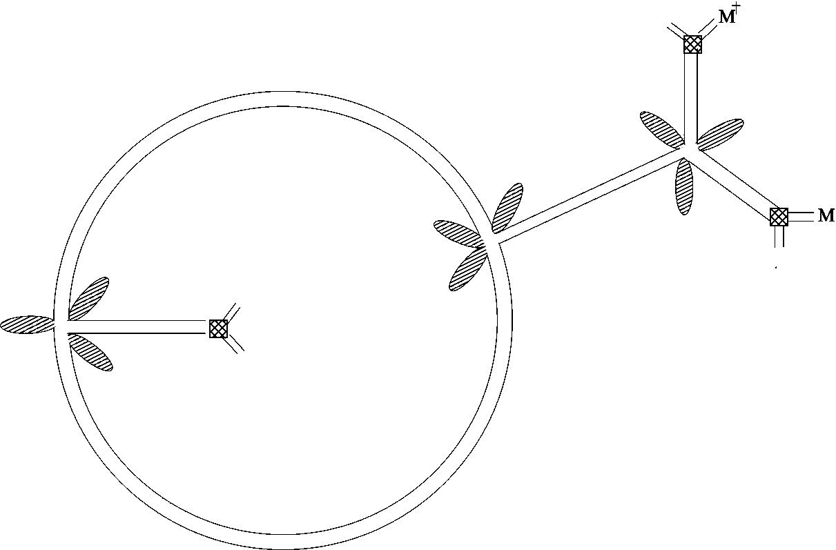
Figure 8: A loop vertex of the theory, bearing 4 derivatives, hence four sources $\sqcup$. We chose $p=5$, hence all vertices are 6-valent. Hatched ellipses represent $A_{p}$ insertions, ribbon edges represent resolvents (there are five such resolvents in this graph) and squares represent derived leaves which can be of three different types $M\sqcup$, $\sqcup M^{\dagger}$ or $\sqcup{\bf{1}}\sqcup$. In the case pictured, we have three squares because two derivatives acted on the same $M^{\dagger}$ factor.

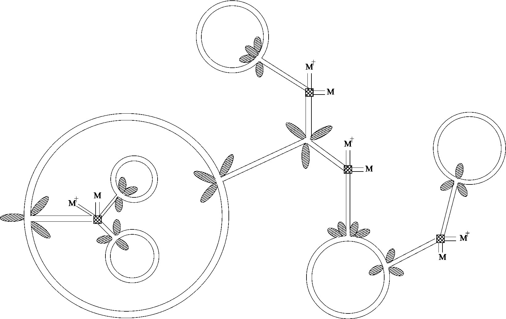
Figure 9: A tree of the loop vertex expansion. It is made of six loop vertices, joined by four edges each bearing a square, which corresponds to the gluing of two $\sqcup$ of the previous picture, and the attentive reader can find seven traces in the drawing.

Similarly a LVE tree is obtained by gluing $n$ such loop vertices through along $n-1$ pairs of glued $\sqcup$ factors, see Figure 9. Beyond the tree, additional cycles between the loop vertices can of course exist but they are hidden in the functional integral $\int dw_{\cal{F}}\int d\mu_{C(x)}$ in (III-55).

D.2 Equivalence at order $\lambda^{2}$ for the effective action for general $p$

The effective action (II-27) reads

$$S = -{\rm Tr}_{\otimes}\log\Big{[}{\bf{1}}_{\otimes}+\lambda\sum_{k=0}^{p-1}A^{k}(X)\otimes A^{p-1-k}(X)\Big{]}$$ (D.124)

$$= \text{Tr}\log\Big{[}\frac{A(X)\otimes 1-1\otimes A(X)}{X\otimes 1-1\otimes X}\Big{]}\,,$$

remember $X=MM^{\dagger}$. Substituting

$$A(\lambda,X) =XT(-\lambda X^{p-1})=X-\lambda X^{p}+p\lambda^{2}X^{2p-1}+O(\lambda^{3})\,,$$ (D.125)

yields

$$S =\lambda S_{1}+\lambda^{2}S_{2}+O(\lambda^{3})$$ (D.126)

with

$$S_{1} =-\sum_{k=0}^{p-1}(\text{Tr}X^{k})(\text{Tr}X^{p-1-k})$$

$$=-2N(\text{Tr}X^{p-1})-\sum_{k=1}^{p-1}(\text{Tr}X^{k})(\text{Tr}X^{p-1-k})$$ (D.127)

$$S_{2} =p\sum_{k=0}^{2p-2}(\text{Tr}X^{k})(\text{Tr}X^{2p-2-k})-\frac{1}{2}\sum_{k,l=0}^{p-1}(\text{Tr}X^{k+l})(\text{Tr}X^{2p-2-k-l})$$

$$=p\sum_{k=0}^{2p-2}(\text{Tr}X^{k})(\text{Tr}X^{2p-2-k})-\sum_{k=0}^{p-2}(k+1)(\text{Tr}X^{k})(\text{Tr}X^{2p-2-k})-\frac{p}{2}(\text{Tr}X^{p-1})^{2}$$

$$=N(2p-1)(\text{Tr}X^{2p-2})+\sum_{k=1}^{p-2}(2p-1-k)(\text{Tr}X^{k})(\text{Tr}X^{2p-2-k})$$

$$+\frac{p}{2}(\text{Tr}X^{p-1})^{2}$$ (D.128)

For example, with $p=3$,

$$S_{1} =-2N\text{Tr}\,X^{2}-(\text{Tr}\,X)^{2}$$ (D.129)

$$S_{2} =5N\text{Tr}\,X^{4}+4(\text{Tr}\,X^{3})(\text{Tr}\,X)+\frac{3}{2}(\text{Tr}X^{2})^{2}.$$ (D.130)

Let us denote by $\langle\cdots\rangle$ the Gaussian averages. The partition function computed with the effective action up to order $O(\lambda^{3})$ reads

$$\big{\langle}\exp S\big{\rangle}=1+\lambda\big{\langle}S_{1}\big{\rangle}+\lambda^{2}\big{\langle}S_{2}\big{\rangle}+\frac{\lambda^{2}}{2}\big{\langle}(S_{1})^{2}\big{\rangle}+O(\lambda^{3})$$ (D.131)

while in conventional perturbation theory it reads

$$\big{\langle}\exp-N\lambda\text{Tr}X^{p}\big{\rangle}=1-\lambda N\big{\langle}\text{Tr}X^{p}\big{\rangle}+\frac{\lambda^{2}N^{2}}{2}\big{\langle}(\text{Tr}X^{p})^{2}\big{\rangle}+O(\lambda^{3})$$ (D.132)

In order to check the equivalence of the two formalisms, it is convenient to use the Schwinger-Dyson equations to decrease the number of traces inside the average,

$$\Big{\langle}\sum_{k+l=p_{1}-1}(\text{Tr}X^{k})(\text{Tr}X^{l})\prod_{i=2}^{n}(\text{Tr}X^{p_{i}})\Big{\rangle}=-\sum_{j=2}^{n}p_{j}\Big{\langle}(\text{Tr}X^{p_{1}+p_{j}-1})$$

$$\prod_{i=2\atop i\neq j}^{n}(\text{Tr}X^{p_{i}})\Big{\rangle}+N\Big{\langle}(\text{Tr}X^{p_{1}}).\prod_{i=2}^{n}(\text{Tr}X^{p_{i}})\Big{\rangle}$$ (D.133)

Establishing the equality of order $\lambda$ terms is an easy task using the Schwinger-Dyson equations with $p_{1}=p$ and $p_{2}=\dots=0$,

$$\big{\langle}S_{1}\big{\rangle} =-\sum_{k=0}^{p-1}\big{\langle}(\text{Tr}X^{k})(\text{Tr}X^{p-1-k})\big{\rangle}=N\Big{\langle}(\text{Tr}X^{p})\Big{\rangle}.$$ (D.134)

At order $\lambda^{2}$, we start with the term with four traces

$$\frac{1}{2}\big{\langle}(S_{1})^{2}\big{\rangle} =\bigg{\langle}\frac{1}{2}\sum_{k=0}^{p-1}(\text{Tr}X^{k})(\text{Tr}X^{p-1-k})\sum_{l=0}^{p-1}(\text{Tr}X^{l})(\text{Tr}X^{p-1-l})\bigg{\rangle}$$

$$=-\sum_{l=0}^{p-1}l\bigg{\langle}(\text{Tr}X^{p-1+l})(\text{Tr}X^{p-1-l})\bigg{\rangle}$$

$$+\frac{N}{2}\Big{\langle}(\text{Tr}X^{p})\sum_{l=0}^{p-1}(\text{Tr}X^{l})(\text{Tr}X^{p-1-l})\Big{\rangle}$$ (D.135)

Let us use the Schwinger-Dyson equations (D.134) again to reduce the three traces term

$$\frac{N}{2}\Big{\langle}(\text{Tr}X^{p})\sum_{l=0}^{p-1}(\text{Tr}X^{l})(\text{Tr}X^{p-1-l})\Big{\rangle} =-\frac{pN}{2}\Big{\langle}(\text{Tr}X^{2p-1})\Big{\rangle}+\frac{N^{2}}{2}\Big{\langle}(\text{Tr}X^{p})(\text{Tr}X^{p})\Big{\rangle}$$ (D.136)

Then, we obtain

$$\frac{1}{2}\big{\langle}(S_{1})^{2}\big{\rangle} =-\sum_{k=0}^{p-2}(p-1-k)\bigg{\langle}(\text{Tr}X^{2p-2-k})(\text{Tr}X^{k})\bigg{\rangle}$$

$$-\frac{pN}{2}\Big{\langle}(\text{Tr}X^{2p-1})\Big{\rangle}+\frac{N^{2}}{2}\Big{\langle}(\text{Tr}X^{p})(\text{Tr}X^{p})\Big{\rangle}$$ (D.137)

Combining all contributions to order $\lambda^{2}$,we are left with

$$\big{\langle}S_{2}\big{\rangle}+\frac{1}{2}\big{\langle}(S_{1})^{2}\big{\rangle} =p\bigg{\langle}\sum_{k=p-1}^{2p-2}(\text{Tr}X^{k})(\text{Tr}X^{2p-2-k})\bigg{\rangle}-\bigg{\langle}\frac{p}{2}(\text{Tr}X^{p-1})^{2}\bigg{\rangle}$$ (D.138)

$$-\frac{pN}{2}\Big{\langle}(\text{Tr}X^{2p-1})\Big{\rangle}+\frac{N^{2}}{2}\Big{\langle}(\text{Tr}X^{p})(\text{Tr}X^{p})\Big{\rangle}$$

We may combine the first two terms on the RHS and use the Schwinger-Dyson equation again,

$$p\bigg{\langle}\sum_{k=p-1}^{2p-2} (\text{Tr}X^{k})(\text{Tr}X^{2p-2-k})\bigg{\rangle}-\bigg{\langle}\frac{p}{2}(\text{Tr}X^{p-1})^{2}\bigg{\rangle}$$

$$=\frac{p}{2}\bigg{\langle}\sum_{k=0}^{2p-2}(\text{Tr}X^{k})(\text{Tr}X^{2p-2-k})\bigg{\rangle}=\frac{pN}{2}\Big{\langle}(\text{Tr}X^{2p-1})\Big{\rangle}.$$ (D.139)

Finally, only the term identical to the conventional perturbative one remains,

$$\big{\langle}S_{2}\big{\rangle}+\frac{1}{2}\big{\langle}(S_{1})^{2}\big{\rangle}=\frac{N^{2}}{2}\Big{\langle}(\text{Tr}X^{p})(\text{Tr}X^{p})\Big{\rangle}\,.$$ (D.140)

D.3 Loop Vertex Expansion and the Standard Perturbation Theory for the quartic interaction case

Let us give a combinatorial proof of the equivalence between our loop vertex expansion formulation and conventional perturbation theory for the quartic case ($p=2$), including terms of order $\lambda^{2}$. In this subsection we return to the case of rectangular matrices $N_{l}$ by $N_{r}$ for the more transparent appearance of the combinatorial factors. Then, (with our convention regarding the symmetry factors and the scaling of the action in $N_{r}$ only), the free energy normalized by the Gaussian one reads

$$\log Z_{\text{perturbation}} =\log\int dMdM^{\dagger}\exp-\big{\{}N_{r}\text{Tr}(MM^{\dagger})+N_{r}\lambda\text{Tr}(MM^{\dagger})^{2}\big{\}}$$

$$=-\lambda\big{\langle}\text{Tr}(MM^{\dagger})^{2}\big{\rangle}+\frac{\lambda^{2}}{2}\big{\langle}\text{Tr}(MM^{\dagger})^{2}\text{Tr}(MM^{\dagger})^{2}\big{\rangle}$$

$$-\frac{\lambda^{2}}{2}\big{\langle}\text{Tr}(MM^{\dagger})^{2}\rangle\langle\text{Tr}(MM^{\dagger})^{2}\big{\rangle}+O(\lambda^{3})$$ (D.141)

This may be expanded over connected oriented ribbon graphs with one or two vertices. These vertices are four-valent, with alternating incoming and out going edges. The first two terms correspond to non necessarily connected maps while the last one subtracts the disconnected part.

Let us describe these graphs and their contributions. The contribution of faces is singled out in the last factor.

With one vertex, we have two double tadpoles (two self-loops on a single vertex), whose contribution is

$$-\frac{\lambda}{N_{r}}\times(N_{l}+N_{r})=-\lambda\frac{N_{l}+N_{r}}{N_{r}}$$ (D.142)

With two vertices, we have ten maps. First the planar and non planar sunshines.

• Sunshine (two vertices joined by four edges, in a planar manner)

  $$\frac{\lambda^{2}}{(N_{r})^{2}}\times(N_{l}N_{r})^{2}=\lambda^{2}(N_{l})^{2}$$ (D.143)

• Twisted sunshine (two vertices joined by four edges, in a non planar manner)

  $$\frac{\lambda^{2}}{(N_{r})^{2}}\times(N_{l}N_{r})=\lambda^{2}\frac{N_{l}}{N_{r}}$$ (D.144)

Then, there are 8 graphs obtained by joining the vertices by two lines and inserting and extra self-loop at each vertex. The latter may be inserted in several manner, on the internal or on the external faces.

• Insertion on the external faces

  $$\frac{\lambda^{2}}{(N_{r})^{2}}\times N_{l}N_{r}(N_{l}^{2}+N_{r}^{2})=\lambda^{2}\frac{N_{l}(N_{l}^{2}+N_{r}^{2})}{N_{r}}$$ (D.145)

• Insertion on the internal faces

  $$\frac{\lambda^{2}}{(N_{r})^{2}}\times N_{l}N_{r}(N_{l}^{2}+N_{r}^{2})=\lambda^{2}\frac{N_{l}(N_{l}^{2}+N_{r}^{2})}{N_{r}}$$ (D.146)

• One on the external and one on the internal faces

  $$\frac{4\lambda^{2}}{(N_{r})^{2}}\times(N_{l}N_{r})^{2}=4\lambda^{2}(N_{l})^{2}$$ (D.147)

  Thus, the logarithm of the partition function reads, in standard perturbation theory,

  $$\log Z_{\text{perturbation}} =-\lambda\frac{N_{l}+N_{r}}{N_{r}}$$

  $$+\lambda^{2}\bigg{(}5(N_{l})^{2}+\frac{N_{l}}{N_{r}}+2\frac{N_{l}(N_{l}^{2}+N_{r}^{2})}{N_{r}}\bigg{)}+O(\lambda^{3})$$ (D.148)

  To check the combinatorial coefficients, let us note that for $N_{l}=N_{r}=1$, one has (including the disconnected piece)

  $$Z=\int dzdz^{\ast}\exp-\big{\{}|z|^{2}+\lambda|z|^{p}\big{\}}=\sum_{n\geq 0}(-\lambda)^{n}\frac{(pn)!}{n!}$$ (D.149)

  This is indeed the case as all contribution to $Z$ sum up to $2$ at order $\lambda$ and to $12$ at order $\lambda^{2}$.

In the LVE, we work with oriented trees on labelled vertices. Performing the contour integral yields decoration of the vertices with effective actions; Each vertex labelled $i$ carries an effective action $S(X_{i})$ ($X_{i}=M_{i}M_{\dagger}$), which writes, in the quartic case (see (D.128) for $p=2$)

$$S(X) =-\lambda(N_{l}+N_{r})(\text{Tr}X)+\lambda^{2}\Big{\{}\frac{3}{2}(N_{l}+N_{r})(\text{Tr}X^{2})+(\text{Tr}X)^{2}\Big{\}}+O(\lambda^{3})$$ (D.150)

At order $\lambda$, there is only the empty tree with a single vertex labelled 1. Its contribution reads

$$\lambda(N_{l}+N_{r})\big{\langle}\text{Tr}(M_{1}M^{\dagger}_{1})\big{\rangle}_{1} =-\lambda N_{l}(N_{l}+N_{r})^{2}$$ (D.151)

with the normalised Gaussian average

$$\big{\langle}\cdots\big{\rangle}_{1} =\int dM_{1}dM^{\dagger}_{1}(\cdots)\exp-N_{r}\text{Tr}(M_{1}M^{\dagger}_{1})$$ (D.152)

At order $\lambda^{2}$, the LVE includes oriented trees with one and two vertices.

• Tree with a single vertex decorated with the order $\lambda^{2}$ effective action and a Gaussian average over a single matrix

  $$\lambda^{2}\Big{\langle}\frac{3}{2}(N_{l}+N_{r})(\text{Tr}X^{2})+(\text{Tr}X)^{2}\Big{\rangle}_{1} =\frac{3}{2}\lambda^{2}\frac{N_{l}(N_{l}+N_{r})^{2}}{N_{r}}+\lambda^{2}N_{l}^{2}+\lambda^{2}\frac{N_{l}}{N_{r}}$$ (D.153)

• Trees with two vertices 1 and 2 and an oriented edge, either from 1 to 2 or from 2 to 1, the two vertices being decorated with the effective action at order 1,

  $$\frac{\lambda^{2}}{2}(N_{l}+N_{r})^{2}\int_{0}^{1}dx\big{\langle}\text{Tr}(M_{1}M_{2}^{\dagger})+\text{Tr}(M_{2}M_{1}^{\dagger})\big{\rangle}_{12} =\frac{\lambda^{2}}{2}\frac{N_{l}(N_{l}+N_{r})^{2}}{N_{r}}$$ (D.154)

  with the Gaussian measure on two matrices of covariance $C_{12}$

  $$\big{\langle}\cdots\big{\rangle}_{12} =\int d\mu_{C_{12}}(M_{1},M^{\dagger}_{1},M_{2},M^{\dagger}_{2})\,(\cdots),\qquad C_{12}=\frac{1}{N_{r}}\begin{pmatrix}1&x\\ x&1\end{pmatrix};$$ (D.155)

Therefore, the LVE expansion yields

$$\log Z_{\text{LVE}} =-\lambda\frac{N_{l}+N_{r}}{N_{r}}+\lambda^{2}\bigg{(}2\frac{N_{l}(N_{l}+N_{r})^{2}}{N_{r}}N_{l}^{2}+\frac{N_{l}}{N_{r}}\bigg{)}+O(\lambda^{3}).$$ (D.156)

Comparing with the perturbative expansion (D.156), we see that $\log Z_{\text{LVE}}=\log Z_{\text{perturbative}}$.

References

- [1] V. Rivasseau, “Constructive Matrix Theory,” JHEP 0709 (2007) 008, arXiv:0706.1224 [hep-th].
- [2] D. Brydges and T. Kennedy, Mayer expansions and the Hamilton-Jacobi equation, Journal of Statistical Physics, 48, 19 (1987).
- [3] A. Abdesselam and V. Rivasseau, “Trees, forests and jungles: A botanical garden for cluster expansions,” arXiv:hep-th/9409094.
- [4] V. Rivasseau and Z. Wang, “How to Resum Feynman Graphs,” Annales Henri Poincaré 15, no. 11, 2069 (2014), arXiv:1304.5913 [math-ph].
- [5] R. Gurau and J. P. Ryan, “Colored Tensor Models - a review,” SIGMA 8, 020 (2012), arXiv:1109.4812 [hep-th].
- [6] R. Gurau, “Random Tensors”, Oxford University Press (2016).
- [7] G. ’t Hooft, “A PLANAR DIAGRAM THEORY FOR STRONG INTERACTIONS,” Nucl. Phys. B 72, 461 (1974).
- [8] R. Gurau, “The 1/N expansion of colored tensor models,” Annales Henri Poincaré 12, 829 (2011), arXiv:1011.2726 [gr-qc].
- [9] R. Gurau and V. Rivasseau, “The 1/N expansion of colored tensor models in arbitrary dimension,” Europhys. Lett. 95, 50004 (2011), arXiv:1101.4182 [gr-qc].
- [10] R. Gurau, “The complete 1/N expansion of colored tensor models in arbitrary dimension,” Annales Henri Poincaré 13, 399 (2012), arXiv:1102.5759 [gr-qc].
- [11] R. Gurau and T. Krajewski, “Analyticity results for the cumulants in a random matrix model,” arXiv:1409.1705 [math-ph].
- [12] R. Gurau, “The 1/N Expansion of Tensor Models Beyond Perturbation Theory,” Commun. Math. Phys. 330, 973 (2014), arXiv:1304.2666 [math-ph].
- [13] T. Delepouve, R. Gurau and V. Rivasseau, “Universality and Borel Summability of Arbitrary Quartic Tensor Models,” arXiv:1403.0170 [hep-th].
- [14] J. Magnen and V. Rivasseau, “Constructive field theory without tears,” Annales Henri Poincaré 9 (2008) 403, arXiv:0706.2457 [math-ph].
- [15] Fang-Jie Zhao, “Inductive Approach to Loop Vertex Expansion”, arXiv:1809.01615.
- [16] R. Gurau and V. Rivasseau, “The Multiscale Loop Vertex Expansion,” Annales Henri Poincaré 16, no. 8, 1869 (2015), arXiv:1312.7226 [math-ph].
- [17] T. Delepouve and V. Rivasseau, “Constructive Tensor Field Theory: The Model,” arXiv:1412.5091 [math-ph].
- [18] V. Lahoche, “Constructive Tensorial Group Field Theory II: The Model,” arXiv:1510.05051 [hep-th].
- [19] V. Rivasseau and F. Vignes-Tourneret, “Constructive tensor field theory: The model,” arXiv:1703.06510 [math-ph].
- [20] V. Rivasseau, “Constructive Tensor Field Theory,” SIGMA 12, 085 (2016), arXiv:1603.07312 [math-ph].
- [21] V. Rivasseau and Z. Wang, “Corrected loop vertex expansion for theory,” J. Math. Phys. 56, no. 6, 062301 (2015), arXiv:1406.7428 [math-ph].
- [22] V. Rivasseau and Z. Wang, “Loop Vertex Expansion for Phi**2K Theory in Zero Dimension,” J. Math. Phys. 51, 092304 (2010), arXiv:1003.1037 [math-ph].
- [23] L. Lionni and V. Rivasseau, “Note on the Intermediate Field Representation of Theory in Zero Dimension”, arXiv:1601.02805.
- [24] L. Lionni and V. Rivasseau, “Intermediate Field Representation for Positive Matrix and Tensor Interactions,” arXiv:1609.05018 [math-ph].
- [25] V. Rivasseau, “Loop Vertex Expansion for Higher Order Interactions,” arXiv:1702.07602 [math-ph].
- [26] G. Gallavotti, “Perturbation Theory”, In: Mathematical physics towards the XXI century, 275-294, R. Sen and A. Gersten, eds., Ber Sheva, Ben Gurion University Press, 1994.
- [27] A. Abdesselam, “The Jacobian conjecture as a problem of perturbative quantum field theory,” Annales Henri Poincaré 4, 199 (2003), math/0208173 [math.CO].
- [28] A. de Goursac, A. Sportiello and A. Tanasa, “The Jacobian Conjecture, a Reduction of the Degree to the Quadratic Case,” Annales Henri Poincaré 17, no. 11, 3237 (2016), ,arXiv:1411.6558 [math.AG].
- [29] A. Abdesselam, “Feynman diagrams in algebraic combinatorics”. Sém. Lothar. Combin. 49 (2002/04), Art. B49c, 45 pp, arXiv:math/0212121.
- [30] B. Eynard, T. Kimura and S. Ribault, “Random matrices,” arXiv:1510.04430 [math-ph].
- [31] V. Rivasseau, “Random Tensors and Quantum Gravity,” SIGMA 12, 069 (2016), ,arXiv:1603.07278 [math-ph].
- [32] W. Mlotkowski and K. A. Penson, “Probability distributions with binomial moments”, in Infinite Dimensional Analysis, Quantum Probability and Related Topics, Vol. 17, No. 2 (2014) 1450014, World Scientific.
- [33] A. D. Sokal, “An Improvement Of Watson’s Theorem On Borel Summability,” J. Math. Phys. 21, 261 (1980).
- [34] Karol A. Penson and Karol Życzkowski. Product of Ginibre matrices: Fuss-Catalan and Raney distributions. Phys. Rev. E, 83:061118, Jun 2011.