Signed counts of
real simple rational functions

Abstract

We study the problem of counting real simple rational functions $\varphi$ with prescribed ramification data (i.e. a particular class of oriented real Hurwitz numbers of genus $0$). We introduce a signed count of such functions which is independent of the position of the branch points, thus providing a lower bound for the actual count (which does depend on the position). We prove (non-)vanishing theorems for these signed counts and study their asymptotic growth when adding further simple branch points. The approach is based on [IZ18] which treats the polynomial case.

1 Introduction

A simple rational function of degree $d$ is a function $\varphi:{\mathbf{C}}{\mathbf{P}}^{1}\to{\mathbf{C}}{\mathbf{P}}^{1}$ which, in affine coordinates, has the form

$$\varphi(z)=\frac{\psi(z)}{z-p}$$

with $\psi\in{\mathbf{C}}[z],\deg(\psi)=d,p\in{\mathbf{C}}$ and $\psi(p)\neq 0$. We call $\varphi$ real if $\psi\in{\mathbf{R}}[z]$ and $p\in{\mathbf{R}}$, and increasing if the leading coefficient of $\psi$ is positive. Two such functions are considered equivalent if they differ by linear coordinate change $z\mapsto\lambda z+\mu,\lambda,\mu\in{\mathbf{R}},\lambda>0$. A unique representative in each equivalence class of increasing functions is given by normalized functions, which are of the form $\varphi(z)=\psi(z)/z$, where $\psi(0)\neq 0$ and the leading coefficient of $\psi$ is $1$.

Let $b_{1},\dots,b_{k}\in{\mathbf{C}}$ be the critical values (also called branch points) of $\varphi$ and let $\Lambda_{1},\dots,\Lambda_{k}$ be the corresponding ramification profiles. This means $\Lambda_{j}=(\Lambda_{j}^{1}\geq\dots\geq\Lambda_{j}^{l_{j}})$ is the partition of $d$ such that $b_{j}$ has $l_{j}$ preimages at which $f$ locally takes the form $z\mapsto z^{\Lambda_{j}^{i}}$. We call $\{(b_{j},\Lambda_{j})\}_{j=1,\dots,k}$ the ramification data of $\varphi$.

Let us now fix $k$ distinct real points ${\mathcal{P}}=(b_{1},\dots,b_{k}),b_{j}\in{\mathbf{R}}$ and $k$ partitions of $d$ $\mathbf{\Lambda}=(\Lambda_{1},\dots,\Lambda_{k})$ and set $d=\sum_{i,j}(\Lambda_{j}^{i}-1)$. We are interested in the number of normalized real simple rational functions $f$ of degree $d$ with ramification data $\{(b_{j},\Lambda_{j})\}_{j=1,\dots,k}$. We denote the set of such functions by ${\mathcal{S}}({\mathcal{P}},\mathbf{\Lambda})$. The number $|{\mathcal{S}}({\mathcal{P}},\mathbf{\Lambda})|$ does not depend on the position of the branch points, as long as we do not change their order of appearance on the real line. However, in general $|{\mathcal{S}}({\mathcal{P}},\mathbf{\Lambda})|$ is not invariant under a permutation of this order. To remedy the situation, we will define a sign $\varepsilon(\varphi)\in\{\pm 1\}$ for any $\varphi\in{\mathcal{S}}({\mathcal{P}},\mathbf{\Lambda})$ (see Definition 1.5) such that the following theorem holds.

Theorem 1.1 (Invariance theorem).

The number

$$\sum_{\varphi\in{\mathcal{S}}({\mathcal{P}},\mathbf{\Lambda})}\varepsilon(\varphi)$$

does not depend on the position of the branch points $b_{1},\dots,b_{k}\in{\mathbf{R}}$. We call it the $S$-number of $\mathbf{\Lambda}$ and denote it by $S(\mathbf{\Lambda})$.

Note that by definition $|S(\mathbf{\Lambda})|$ gives a lower bound for $|{\mathcal{S}}({\mathcal{P}},\mathbf{\Lambda})|$. It is therefore interesting to find criteria for $S(\mathbf{\Lambda})\neq 0$ (equivalent to the existence of functions) or to prove statements about the asymptotic growth. To formulate our results, we need the following notation. For a partition $\Lambda=(\Lambda^{1},\dots,\Lambda^{t})$ of $d$, the reduced partition $\lambda$ is the partition obtained from $(\Lambda^{1}-1,\dots,\Lambda^{t}-1)$ after removing all zeros. A branch point is called simple if its reduced ramification profile is $\lambda=(1)$. Let us now fix $k$ decreasing finite sequences ${\bm{\lambda}}=(\lambda_{1},\dots,\lambda_{k})$ and $m\in{\mathbf{N}}$. We set

$$d:=m+\sum_{i,j}\lambda_{j}^{i},\vspace{-1.5ex}$$

and let $\mathbf{\Lambda}=(\Lambda_{1},\dots,\Lambda_{k+m})$ be the unique collection of partitions of $d$ such that $\Lambda_{1},\dots,\Lambda_{k}$ reduce to $\lambda_{1},\dots,\lambda_{k}$ and $\Lambda_{k+1}=\dots=\Lambda_{k+m}$ reduce to $(1)$. Hence $S({\bm{\lambda}},m):=S(\mathbf{\Lambda})$ is the $S$-number of normalized simple rational functions with $k+m$ branch points, $k$ of which have reduced ramification profiles $\lambda_{1},\dots,\lambda_{k}$ while the remaining $m$ branch points are simple. We collect these numbers in two generating series, separately for $d$ odd and even:

$$F^{\text{odd}}_{\bm{\lambda}}(q)=\sum_{\begin{subarray}{c}m=0\\ d\text{ odd}\end{subarray}}^{\infty}S({\bm{\lambda}},m)\frac{q^{m}}{m!},\quad\quad F^{\text{even}}_{\bm{\lambda}}(q)=\sum_{\begin{subarray}{c}m=0\\ d\text{ even}\end{subarray}}^{\infty}S({\bm{\lambda}},m)\frac{q^{m}}{m!}.$$

Theorem 1.2 ((Non-)Vanishing theorem).

The generating series $F^{\text{odd}}_{\bm{\lambda}}(q)$ is not identically zero if and only if the following conditions hold:

• In each partition $\lambda_{j}$ at most one odd number appears an odd number of times and at most one even number appears an odd number of times.

• There exists an even number of partitions $\lambda_{j}$ having exactly one even number appearing an odd number of times.

The generating series $F^{\text{even}}_{\bm{\lambda}}(q)$ is not identically zero if and only if the following conditions hold:

• In each partition $\lambda_{j}$ at most one odd number appears an odd number of times and at most one even number appears an odd number of times.

Theorem 1.3 (Logarithmic growth).

Fix ${\bm{\lambda}}=(\lambda_{1},\dots,\lambda_{k})$ and the parity of $d$ such that the non-vanishing criteria in Theorem 1.2 are satisfied. Set $\pi\equiv d-\sum_{i,j}\lambda_{j}^{i}\mod 2$ the corresponding parity of $m$. Then the logarithmic growth of $S({\bm{\lambda}},m)$ in $m$ is given by

$$\ln|S({\bm{\lambda}},m)|\underset{\begin{subarray}{c}m\to\infty\\ m\equiv\pi\mod 2\end{subarray}}{\sim}m\ln(m).$$

These statements should be compared to [IZ18, Theorems 1,3,4,5] in the polynomial case.

Let $H^{\mathbf{C}}({\bm{\lambda}},m)$ denote the Hurwitz number counting complex simple rational functions $\varphi\in{\mathbf{C}}(z)$ with $k$ critical levels of reduced ramification type $\lambda_{1},\dots,\lambda_{k}$ and $m$ additional simple branch points. Note that $\ln H^{\mathbf{C}}({\bm{\lambda}},m)\sim m\ln(m)$ for $m\to\infty$ (see Remark 8.13), so under the conditions of the theorem the real and complex counts are logarithmically equivalent.

Since all the main theorems crucially depend on the definition of the signs $\varepsilon(\varphi)$, let us insert its definition here.

Definition 1.4.

Let $\Sigma=(a_{1},\dots,a_{n})$ be a finite sequence of integers. A disorder of $\Sigma$ is a pair $i<j$ such that $a_{i}>a_{j}$. The number of disorders is denoted by $\operatorname{dis}(\Sigma)$.

For any $a\in{\mathbf{C}}$ we denote by $R_{\varphi}(a)\in{\mathbf{N}}$ the ramification index of $\varphi$ at $a$, i.e. the order of vanishing of $\varphi(z)-\varphi(a)$ for $a\neq p$, and $R_{\varphi}(p)=1$.

Definition 1.5.

Let $\varphi$ be a real simple rational function with simple pole $p$ and let $b$ be a branch point of $\varphi$. We set $\Sigma_{b}$ to be the sequence of ramification indices $R_{\varphi}(a)$ for $a\in(\varphi^{-1}(b)\cap{\mathbf{R}})\sqcup\{p\}$, ordered according to their appearance on the real line. Let $b_{1},\dots,b_{k}$ denote the collection of branch points of $\varphi$. The sign of $\varphi$ is

$$\varepsilon(\varphi):=(-1)^{\operatorname{dis}(\varphi)}\quad\quad\text{where }\operatorname{dis}(\varphi):=\operatorname{dis}(\Sigma_{b_{1}})+\dots+\operatorname{dis}(\Sigma_{b_{k}}).$$

Remark 1.6.

The main difference with [IZ18] is that our definition considers the simple pole $p$ as part of the preimage for any critical level. It will become clear in Section 3 that this is, under some assumptions, the only definition with a chance to satisfy to Theorem 1.1. We call the disorders involving $p$ pole disorders and all other ones level disorders.

Let us give a brief outline of the paper. In Sections 2, 3 and 4 we closely follow the approach in [IZ18] to prove the Invariance Theorem 1.1 using dessins d’enfant. The main difference in these sections is that instead of trees we deal with graphs with a loop. Our presentation focuses on the difference to loc. cit. while being mostly self-contained. Sections 5, 7 and 8 deal with Theorems 1.2 and 1.3. Here, the differences to loc. cit. are more significant. In particular, in Section 6 we introduce the generating series of broken alternations, show that it obeys a certain differential equation and use this to express it in terms of the generating series of (ordinary) alternations. This is crucial for the extension of the ideas from loc. cit. to the case of simple rational functions.

The counts of simple rational functions under investigation here can be considered as oriented versions of real Hurwitz numbers as defined for example in [MR15, GMR16]. The approach to study these numbers via an invariant signed count is in the spirit of Welschinger invariants [Wel05, IKS04], even though the definition of Welschinger signs is of different flavour than Definition 1.5. Real Hurwitz numbers and their invariance/asymptotic properties have also been studied in the context of topological quantum field theories, matrix models, moduli spaces of real algebraic curves [AN06, GZ15, Orl17], however, mostly in the context of completely imaginary configurations of branch points ${\mathcal{P}}$, in contrast to the completely real configurations ${\mathcal{P}}\subset{\mathbf{R}}{\mathbf{P}}^{1}$ we consider here.

2 Dessins d’enfant for simple rational functions

Conjugation-invariant dessins d’enfant are used to describe real functions in [Bar92, NSV02, IZ18] (for generic polynomials, generic rational functions and arbtirary polynomials, respectively). The following definition is adapted to describe the simple rational functions considered in this paper.

We fix $d$ and a sequence $\mathbf{\Lambda}=(\Lambda_{1},\ldots,\Lambda_{k})$ of partitions of $d$ such that $d=\sum_{i,j}(\Lambda_{j}^{i}-1)$. Note that this implies $k>1$. For a partition $\Lambda$ we denote by $l(\Lambda)$ the number of parts of $\Lambda$. For the vertex $v$ of a graph $G$, its degree $\deg(v)$ is the number of adjacent half edges. Throughout the following, we fix an affine chart ${\mathbf{C}}{\mathbf{P}}^{1}={\mathbf{C}}\sqcup\{\infty\}$ and use the orientation on ${\mathbf{R}}{\mathbf{P}}^{1}$ induced by the increasing orientation on ${\mathbf{R}}$.

Definition 2.1.

A real simple rational dessin of degree $d$ and type $\mathbf{\Lambda}$ is a graph $\Gamma\subset{\mathbf{C}}{\mathbf{P}}^{1}$ whose vertices are labelled by elements of the set $\{1,\ldots,k,\infty\}$ such that the following conditions hold.

1. The labelled graph $\Gamma$ is invariant under complex conjugation $\operatorname{conj}$.

2. The real circle ${\mathbf{R}}{\mathbf{P}}^{1}$ is a union of edges of $\Gamma$.

3. Exactly two vertices of $\Gamma$ are labelled by $\infty$, namely $P:=\infty\in{\mathbf{C}}{\mathbf{P}}^{1}$ and $p\in{\mathbf{R}}$, with $\deg(P)=2d-2$ and $\deg(p)=2$.

4. For each integer $1\leq j\leq k$, the graph $\Gamma$ has exactly $l(\Lambda_{j})$ vertices labelled by $j$ and their degrees are equal to the elements of $\Lambda_{j}$, multiplied by $2$.

5. Each edge of $\Gamma$ is one of the following $k+1$ types: $\infty\rightarrow 1$, $1\rightarrow 2$, $2\rightarrow 3$, $\ldots$, $k-1\rightarrow k$, $k\rightarrow\infty$; in particular, this induces an orientation on $\Gamma$.

6. For any connected component $C$ of ${\mathbf{C}}{\mathbf{P}}^{1}\setminus\Gamma$, each type of edges appears exactly once in the boundary $\partial C$ of $C$.

7. There exists an edge in ${\mathbf{R}}{\mathbf{P}}^{1}$ of type $k\to\infty$ whose orientation agrees with that of ${\mathbf{R}}{\mathbf{P}}^{1}$.

Remark 2.2.

Given a real dessin $\Gamma\subset{\mathbf{C}}{\mathbf{P}}^{1}$, we call $\Gamma\setminus\{P\}\subset{\mathbf{C}}$ the affine dessin for $\Gamma$. It is a graph with $2d-2$ unbounded ends of type $\infty\to 1$ or $k\to\infty$, and it is easy to adapt the above conditions into affine versions such that both contain exactly the same information. We will mostly use affine dessins in our figures. An example for $d=21,k=4$ is given in Figure 7. The vertex $p$ is drawn in red.

It is easy to associate a real simple rational dessin $\Gamma_{\varphi}$ to any increasing real simple rational function $\varphi$ with branch points $b_{1}<\dots<b_{k}\in{\mathbf{R}}$. As a set, we define $\Gamma_{\varphi}:=\varphi^{-1}({\mathbf{R}}{\mathbf{P}}^{1})$. We label the two preimages of $\infty\in{\mathbf{C}}{\mathbf{P}}^{1}_{\text{target}}$ by $\infty$ and the preimages of $b_{j}$ by $j$.

Definition 2.3.

Two real simple rational dessins $\Gamma,\Gamma^{\prime}$ are equivalent if there exists a homeomorphism $\Phi:{\mathbf{C}}{\mathbf{P}}^{1}\to{\mathbf{C}}{\mathbf{P}}^{1}$ such that $\Phi$ and $\operatorname{conj}$ commute, $\Phi|_{{\mathbf{R}}{\mathbf{P}}^{1}}$ is orientation-preserving, $\Phi(\Gamma)=\Gamma^{\prime}$ and $\Phi$ preserves the labels. We denote the set of equivalence classes by $\operatorname{Des}(\mathbf{\Lambda})$.

Theorem 2.4.

Fix arbitrary real points ${\mathcal{P}}=\{b_{1}<\dots<b_{k}\}\in{\mathbf{R}}{\mathbf{P}}^{1}$. Then the map

$${\mathcal{S}}({\mathcal{P}},\mathbf{\Lambda})\to\operatorname{Des}(\mathbf{\Lambda}),\quad\varphi\mapsto[\Gamma_{\varphi}],$$

is a bijection.

Proof.

The proof is a straightforward application of dessins d’enfant and the Riemann existence theorem and can be easily adapted from [IZ18, Propositions 2.6 and 2.7]. ∎

Remark 2.5.

We define the sign of dessin to be the sign of the associated rational function, $\epsilon(\Gamma_{\varphi})=\epsilon(\varphi)$. Note that $\epsilon(\Gamma_{\varphi})$ can be easily read of from the dessin itself since the sequence $\Sigma_{b_{j}}$ of ramification indices for the branch point $b_{j}$ is equal to the sequence of degrees of the vertices labelled by $i$ plus the pole $p$ divided by $2$ (cf. Definition 1.5).

3 Bipartite graphs

In this section, we introduce auxiliary combinatorial objects that are used in the proof of the invariance theorem. They are equivalent to simple rational dessins with $k=2$ critical values.

Definition 3.1.

A black and white simple graph, or short, $bw$-graph is a connected graph $G$ embedded into ${\mathbf{C}}$ whose vertices are coloured in black and white in alternation, and it has only one cycle of edge length $2$ (see Figure 1). A $bw$-graph is said to be real if it is invariant (including the colours) under complex conjugation. Two (real) $bw$-graphs are isomorphic if one can be transformed into the other by an ($\operatorname{conj}$-equivariant) homeomorphism of ${\mathbf{C}}$ (that preserves the orientation of ${\mathbf{R}}$).

For a real $bw$-graph $G$ the real part is ${\mathbf{R}}G:=G\cap{\mathbf{R}}$. The leftmost and rightmost vertices of ${\mathbf{R}}G$ are called the border vertices. The graph is called white-sided (respectively black-sided) if its rightmost border vertex is white (respectively, black). It is called short if the the cycle of $G$ contains a border vertex. Otherwise, we call it long.

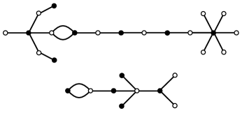
Figure 1: Two real $bw$-graphs.

We denote by $(\Sigma_{w},\Sigma_{b})$ the sequence of degrees of its real white and real black vertices, respectively, from left to right. A level disorder is a disorder in one of these sequences, while a pole disorder is real vertex of $G$ to the left of the cycle and with degree larger than $1$ (including the left cycle vertex). In this section, it is more convenient to keep track of level and pole disorders separately. We denote them by $\operatorname{lev}(G)$ and $\operatorname{pol}(G)$, respectively. The sign of $G$ is

$$\varepsilon(G)=(-1)^{\operatorname{lev}(G)+\operatorname{pol}(G)}.$$

Example 3.2.

The real $bw$-graph appearing at the top of Figure 1 is a white-sided long graph. It has $(\Sigma_{w},\Sigma_{b})=(132221,43226)$ and its sign is equal to $(-1)^{\displaystyle 12+2}=+1$.
The real $bw$-graph $G$ appearing at the bottom of Figure 1 is a black-sided short graph. It has $(\Sigma_{w},\Sigma_{b})=(34,223)$ and its sign is equal to $(-1)^{\displaystyle 0+1}=-1$.

Remark 3.3.

A vertex of $G$ is called even or odd if its degree $\deg(v)$ is even or odd, respectively. A real $bw$-graph $G$ can have four, two or zero real odd vertices. Only the first case is equivalent to $G$ being long. Note that in this case not all four vertices have the same colour.

For the rest of this section, we fix a positive integer $d$, and two partitions $\Lambda_{w},\Lambda_{b}$ of $d$. We denote by $\bm{G}$ the set of real $bw$-graphs such that the degrees of their white and black vertices give $\Lambda_{w}$ and $\Lambda_{b}$, respectively. We split $\bm{G}=\bm{W}\sqcup\bm{B}$ into the subsets of white-sided and black-sided graphs, respectively.

Convention 3.4.

Let $M$ be a set together with a sign function $\varepsilon:M\to\{\pm 1\}$. We set

$$S(M):=\sum_{x\in M}\varepsilon(x).$$

Theorem 3.5.

Fix a positive integer $d$ and two partitions $\Lambda_{w}$ and $\Lambda_{b}$ of $d$. Then

$$S(\bm{W})=S(\bm{B}).$$

Example 3.6.

Figure 2 shows all graphs with $\Lambda_{w}=(3,2,1,1)$ and $\Lambda_{b}=(3,2,2)$. The sum of signs is equal to 2 both for the black-sided graphs on top and for the white-sided graphs on the bottom.

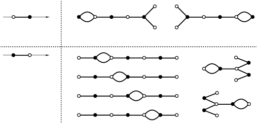
Figure 2: An example of $S(\bm{W})=S(\bm{B})$ for $\Lambda_{w}=(3,2,1,1)$ and $\Lambda_{b}=(3,2,2)$.

3.1 Symmetrizing graphs

To prove Theorem 3.5, we subsequently identify subsets of graphs which cancel each other, hence reducing the problem to special classes of graphs. The first step is to symmetrize graphs in a certain sense.

Definition 3.7.

Let $v$ be a real vertex of the graph $G$. A pair of trees $T$ growing at $v$ is a pair of complex conjugated connected components $T=(\Theta,\overline{\Theta})$ of $G\setminus\{v\}$ with $\Theta\neq\overline{\Theta}$. Let $T_{1},\dots,T_{k}$ be the sequence of all pairs of trees growing at $v$, ordered according to their appearance in $\{z:\Im(z)>0\}\subset{\mathbf{C}}$ following the clock-wise direction (see Figure 3). Then the forest growing at $v$ is the sequence $F(v)=(T_{1},\dots,T_{k-1})$ if $v$ is an odd border vertex and $F(v)=(T_{1},\dots,T_{k})$ otherwise.

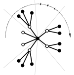
Figure 3: Ordering of the pairs of non-real trees growing at $v$.

Let $l(v)$ denote the number of entries of $F(v)$. If $v$ is even, then $\deg(v)=2k+2=2l(v)+2$. If $v$ is odd, then $\deg(v)=2k+1$ or $\deg(v)=2k+3$ depending on whether $v$ is a border vertex or not. Due to the shortening of $F(v)$ for border vertices we obtain $\deg(v)=2l(v)+3$ for any odd vertex with $\deg(v)\neq 1$.

Definition 3.8.

A collection of real vertices $v_{1},\dots,v_{k}$ of a given graph $G$ are of the same type if they are of the same colour, the same parity and $\deg(v_{i})>1$ for all $i$. Given a permutation $\sigma$ of the $v_{i}$, we obtain a new graph $\sigma(G)$ by cutting off the forest $F(v_{i})$ from $v_{i}$ and replanting it at $v_{\sigma(v_{i})}$, for all $i$. Hereby we keep the order of the individual pairs of trees in $F(v_{i})$ and the position of the (fixed) right-most pair of trees in the case of a odd border vertex (see Figure 4). This determines $\sigma(G)$ uniquely up to homeomorphism. In the case of two vertices $v_{1},v_{2}$ and $\sigma$ the transposition, we call the result the flipped graph $\operatorname{Flip}_{v_{1}}^{v_{2}}(G)$.

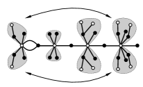
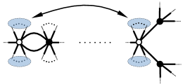
Figure 4: Exchanging forests for even and odd vertices, respectively.

Note that in terms of the real sequences of $G$ the operation $\operatorname{Flip}_{v_{1}}^{v_{2}}$ acts like a transposition permuting the two entries corresponding to $v_{1}$ and $v_{2}$.

Definition 3.9.

Let $\Sigma=(e_{1},\dots,e_{2m})$ be an integer sequence $\Sigma$ of even length $2m$. Then $\Sigma$ is symmetric if $e_{m-k}=e_{m+k+1}$ for all $k=0,\dots,m-1$. If $\Sigma$ is not symmetric, the first non-symmetric pair denotes the unique pair $(m-k,m+k+1)$ such that $e_{m-k}\neq e_{m+k+1}$ and $(e_{m-k+1},\dots,e_{m+k})$ is symmetric.

A (general) integer sequence $\Sigma$ is nearly symmetric if it is symmetric after applying the following two steps:

• Remove all $1$’s.

• If the resulting sequence is of odd length, remove the first entry.

If $\Sigma$ is not nearly symmetric then the first non-symmetric pair is the pair of indices which corresponds to the first non-symmetric pair after applying the same two steps.

Given an integer sequence $\Sigma$, we denote by $\Sigma^{{\text{even}}}$ and $\Sigma^{{\text{odd}}}$ the subsequence of even and odd entries, respectively. A real $bw$-graph $G$ is nearly symmetric if all the sequences $\Sigma^{{\text{even}}}_{w},\Sigma^{{\text{odd}}}_{w},\Sigma^{{\text{even}}}_{b},\Sigma^{{\text{odd}}}_{b}$ are nearly symmetric separately. If $G$ is not nearly symmetric, then the first non-symmetric pair is the pair of vertices corresponding to the first non-symmetric pair for the first sequence from before (in the given order) which is not nearly symmetric.

Remark 3.10.

Let us unravel the previous definition in the given situation. Let $\Sigma^{{\text{even}}}$ be a nearly symmetric sequence of only even entries, then either it is of the form $(e_{1},\dots,e_{m},e_{m},\dots,e_{1})$ or $(e_{0},e_{1},\dots,e_{m},e_{m},\dots,e_{1})$. Let $\Sigma^{{\text{odd}}}$ be a sequence of only odd entries and of length at most $3$ and not of the form $(1,1)$ or $(x,1,y)$ (which cannot appear in practice). Then it is nearly symmetric if and only if it is of one of the following forms (where we assume $a\neq 1\neq b$).

$$\emptyset,(a),(1),(a,a),(a,1),(1,a),(1,a,1),(a,a,1),(1,a,a),(a,b,b)$$

If $\Sigma^{{\text{odd}}}$ is not nearly symmetric, it is of the form $(\underline{c},\underline{d})$, $(\underline{c},\underline{d},1)$, $(1,\underline{c},\underline{d})$, $(a,\underline{c},\underline{d})$ with $c\neq d$. The first non-symmetric pair is formed by the underlined entries.

Example 3.11.

The top graph in Figure 1 is not nearly symmetric and its first non-symmetric pair is formed by the left- and right-most black vertex of degree $4$ and $6$, respectively. The bottom graph is nearly symmetric.

Lemma 3.12.

Let $G$ be a graph which is not nearly symmetric and let $v_{1}<v_{2}$ be the first non-symmetric pair of $G$. Then

$$\varepsilon(\operatorname{Flip}_{v_{1}}^{v_{2}}(G))=-\varepsilon(G).$$

Proof.

Let $\Sigma$ be the sequence of degrees of some colour and parity as $v_{1},v_{2}$. If $\deg v_{1}$ and $\deg v_{2}$ are consecutive entries of $\Sigma$, flipping the two obviously changes the number of disorders by $1$. If not consecutive, they are separated by a stretch of the form $(e_{1},\dots,e_{m},e_{m},\dots,e_{1})$. Such a stretch can be removed without changing the parity of $\operatorname{dis}(\Sigma)$, since any disorder involving the stretch shows up an even number of times. Hence the previous case applies. The pole disorders are not affected by the flipping. ∎

Proposition 3.13.

Consider the subsets $\bm{N\!W}\subset\bm{W}$ and $\bm{N\!B}\subset\bm{B}$ of nearly symmetric white-sided and black-sided graphs, respectively. Then we have

$$S(\bm{W})=S(\bm{N\!W}),\quad\quad S(\bm{B})=S(\bm{N\!B}).$$ (1)

Proof.

We define the involution $\operatorname{Sym}:\bm{W}\setminus\bm{N\!W}\to\bm{W}\setminus\bm{N\!W}$ by setting $\operatorname{Sym}(G)=\operatorname{Flip}_{v_{1}}^{v_{2}}(G)$, where $v_{1}<v_{2}$ is the first non-symmetric pair of $G$. By Lemma 3.12 the pairs $G,\operatorname{Sym}(G)$ cancel out in $S(\bm{W})$ and the statement follows. ∎

3.2 Rotating and shifting vertices

The next step is based on rotating graphs by $180^{\circ}$. This operation reverses the real sequences. In order to stay in the class of nearly symmetric graphs, we need to make a slight adjustment.

Definition 3.14.

Let $v_{1}<\ldots<v_{k}$ be a collection of ordered real vertices of the same type and let $\sigma=(v_{1}\dots v_{k})$ be the cyclic permutation of these vertices. The cyclic shift of $G$ based on $v_{1}<\ldots<v_{k}$ is the graph $\sigma(G)$ (see Definition 3.8 and Figure 5).

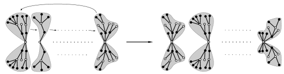
Figure 5: The cyclic shift operation.

Remark 3.15.

Let $\Sigma$ be a nearly symmetric sequence and let $\Sigma^{\prime}$ be the reversed sequence. Then either $\Sigma^{\prime}$ is nearly symmetric or can be made nearly symmetric by cyclically shifting all non-one entries of $\Sigma^{\prime}$ to the next non-one entry (keeping all $1$’s fixed). Obviously, if $\Sigma^{\prime}$ is part of the real sequence of a graph $G$, then the shifting, if necessary, can be performed by the cycled shifting operation based on the vertices corresponding to the non-one entries of $\Sigma^{\prime}$.

We set $\bm{N\!G}=\bm{N\!W}\cup\bm{N\!B}$.

Definition 3.16.

We define the map $\operatorname{Rot}:\leavevmode\nobreak\ \bm{N\!G}\to\bm{N\!G}$, where $\operatorname{Rot}(G)$ is the graph obtained from $G$ by a rotation of $180^{\circ}$ and, if necessary, performing cyclic shifts based on the higher-valent vertices of certain colour and parity (see Remark 3.15).

Lemma 3.17.

Let $G$ be a nearly symmetric graph and let $\Sigma$ be its real sequence of white (or black) vertices. Let $\operatorname{Rot}(\Sigma)$ denote the real sequence of white (or black) vertices of $\operatorname{Rot}(G)$. Set $l:=l(\Sigma^{{\text{even}}})$. Then we have

$$\operatorname{dis}(\operatorname{Rot}(\Sigma))-\operatorname{dis}(\Sigma)\equiv\begin{cases}0&\Sigma^{{\text{odd}}}=\emptyset\text{ or }(a,a),\\ 1&\Sigma^{{\text{odd}}}=(1,a)\text{ or }(a,1),\\ l&\text{otherwise},\end{cases}\mod 2.$$

Here we refer to the ten possible forms for $\Sigma^{{\text{odd}}}$ introduced in Remark 3.10.

Proof.

We set $\overline{\Sigma}=\operatorname{Rot}(\Sigma)$. As in Lemma 3.12, throughout the proof we will use the fact that a consecutive pair of identical entries in $\Sigma$ can be removed without changing the parity of $\operatorname{dis}(\Sigma)$. We first focus on $\Sigma^{{\text{odd}}}$. Going through the ten types in Remark 3.10 we can easily check that $\operatorname{dis}(\overline{\Sigma}^{{\text{odd}}})-\operatorname{dis}(\Sigma^{{\text{odd}}})\equiv 1$ only if $\Sigma^{{\text{odd}}}=(1,a)$ or $(a,1)$ and $\operatorname{dis}(\overline{\Sigma}^{{\text{odd}}})-\operatorname{dis}(\Sigma^{{\text{odd}}})\equiv 0$ otherwise.

We now reduce to this case by the following trick: Let $k$ be the number of transposition necessary to transform $\Sigma$ into $(\Sigma^{{\text{odd}}},\Sigma^{{\text{even}}})$ (i.e. moving all odd entries to the beginning of the sequences). Since each of these transpositions flips an odd and even entry (i.e., two non-equal numbers), we get $\operatorname{dis}(\Sigma)\equiv\operatorname{dis}((\Sigma^{{\text{odd}}},\Sigma^{{\text{even}}}))+k$. The pattern of odd and even entries in $\overline{\Sigma}$ is reversed to the pattern of $\Sigma$ (the cyclic shifts only permute odd and even entries separately). Hence moving all odd entries in $\overline{\Sigma}$ to the right, we get $\operatorname{dis}(\overline{\Sigma})\equiv\operatorname{dis}((\overline{\Sigma}^{{\text{even}}},\overline{\Sigma}^{{\text{odd}}}))+k$. If we set $m:=l(\Sigma^{{\text{odd}}})$ and move all the odd entries back to the left, we get $\operatorname{dis}(\overline{\Sigma})\equiv\operatorname{dis}((\overline{\Sigma}^{{\text{odd}}},\overline{\Sigma}^{{\text{even}}}))+k+lm$. Putting things together, we obtain

$$\operatorname{dis}(\operatorname{Rot}(\Sigma))-\operatorname{dis}(\Sigma) \equiv\operatorname{dis}((\overline{\Sigma}^{{\text{odd}}},\overline{\Sigma}^{{\text{even}}}))-\operatorname{dis}((\Sigma^{{\text{odd}}},\Sigma^{{\text{even}}}))+lm$$

$$\equiv\operatorname{dis}(\overline{\Sigma}^{{\text{odd}}})-\operatorname{dis}(\Sigma^{{\text{odd}}})+lm.$$ (2)

Plugging in the possible types for $\Sigma^{{\text{odd}}}$, the claim follows. ∎

Lemma 3.18.

Let $G\in\bm{N\!G}$ be a nearly symmetric graph. We have $\varepsilon(\operatorname{Rot}(G))=-\varepsilon(G)$ if there exists a sequence $\Sigma_{c}^{{\text{odd}}}(G)$ of $G$ of some colour $c$ such that $\Sigma_{c}^{{\text{odd}}}(G)=(1,b,b)$, $(b,b,1)$, or $(1)$, and $\varepsilon(\operatorname{Rot}(G))=\varepsilon(G)$ otherwise.

Proof.

Without loss of generality, we shall restrict to white-sided graphs. A white-sided graph with the left border vertex being white (resp. black) will be referred to as a white-white (resp. black-white) graph.

The total number of real vertices is odd for white-white graphs and even for black-white graphs. Let $q$ be the number of one-valent real vertices, then

$$\operatorname{pol}(\operatorname{Rot}(G))-\operatorname{pol}(G)\equiv\begin{cases}q+1\mod 2,&\text{if\leavevmode\nobreak\ }G\text{ is a white-white graph},\\ q\mod 2,&\text{if\leavevmode\nobreak\ }G\text{ is a black-white graph}.\end{cases}$$ (3)

This is true since each real vertex of $G$ with $\deg(v)\neq 1$ contributes either to $\operatorname{pol}(G)$ or, after rotation, to $\operatorname{pol}(\operatorname{Rot}(G))$.

For the case of white-white graphs, the sequences $\Sigma^{{\text{odd}}}_{w}$ and $\Sigma^{{\text{odd}}}_{b}$ have both odd length, and thus Lemma 3.17 implies $\operatorname{lev}(\operatorname{Rot}(G))\equiv\operatorname{lev}(G)+p\equiv\operatorname{lev}(G)+1$. Here $p$ is the total number of even real vertices. Together with Equation (3), we get $\varepsilon(\operatorname{Rot}(G))=(-1)^{q}\varepsilon(G)$. Hence the sign changes if and only if $\Sigma^{{\text{odd}}}_{w}$ is of type $(1,b,b)$, $(b,b,1)$, or $(1)$.

In the case of black-white graphs, each of $\Sigma^{{\text{odd}}}_{w}$ and $\Sigma^{{\text{odd}}}_{b}$ has even length. Both, only one or none of them can be of type $(1,a)$ or $(a,1)$, corresponding to $q=2,1$ or $0$. Lemma 3.17 implies $\operatorname{lev}(\operatorname{Rot}(G))\equiv\operatorname{lev}(G)+q$. Together with Equation (3) this gives $\varepsilon(\operatorname{Rot}(G))=(-1)^{2q}\varepsilon(G)=\varepsilon(G)$, which proves the claim. ∎

Remark 3.19.

A simple parity check shows the following: If $d$ is even, all graphs in $\bm{G}$ have border vertices of opposite colour. If $d$ is odd, all graphs in $\bm{G}$ have border vertices of the same colour.

Proof of Theorem 3.5 for $d$ even.

Rotation defines a bijection $\operatorname{Rot}:\bm{NW}\to\bm{NB}$ with $\varepsilon(G)=\varepsilon(\operatorname{Rot}(G))$ by Lemma 3.18. Then Proposition 3.13 finishes the proof. ∎

Definition 3.20.

A reduced graph $G$ is a nearly symmetric graph such that $\Sigma_{w}^{{\text{odd}}}$ and $\Sigma_{b}^{{\text{odd}}}$ are of the form $(a),(1,a,1),$ or $(a,b,b)$ for $a,b\neq 1$. We denote by $\bm{RW}\subset\bm{N\!W}$ the subset of reduced white-sided graphs.

Corollary 3.21.

If $d$ is odd, we have $S(\bm{W})=S(\bm{RW})$.

Proof.

Rotation defines an involution on $\bm{NW}\setminus\bm{RW}$ which satisfies $\varepsilon(G)=-\varepsilon(\operatorname{Rot}(G))$ by Lemma 3.18. Using Proposition 3.13 we get $S(\bm{RW})=S(\bm{NW})=S(\bm{W})$. ∎

3.3 Midline operation and rest of the proof

In this subsection we assume $d$ odd and set $\bm{RG}=\bm{RW}\cup\bm{RB}$. We want to construct a bijective correspondence

$$\operatorname{Tr}:\leavevmode\nobreak\ \{\text{\emph{short} graphs of}\leavevmode\nobreak\ \bm{RG}\}\longrightarrow\{\text{\emph{long} graphs of}\leavevmode\nobreak\ \bm{RG}\}$$

which does not necessarily respect the colour of a graph.

Construction 3.22.

Without loss of generality, consider a white-sided short graph $G=G_{0}\in\bm{RW}$ and assume that the cycle lies on the left hand side of $G$ (see bottom graph of Figure 1).

1. We use the midline cutting method from [IZ18, Proof of Lemma 3.13]: Take the pair of trees growing at the right border vertex closest to the positive direction of the real axis and cut each tree into two halves along the midline (see Figure 6). Glue the two $\operatorname{conj}$-symmetric halves closest to the real axis to obtain a rooted tree which we attach to the left border vertex of $G$ such that the glued midline is mapped to ${\mathbf{R}}$. Do the same with the second pair of half-trees, but attaching them to the right border vertex. The long graph obtained by this construction is denoted by $G_{1}$.

2. The graph $G_{1}$ is in general not of type $\Lambda_{w},\Lambda_{b}$, since the former border vertices $v_{1},v_{2}$ changed their degree. We repair this by applying $G_{2}:=\operatorname{Flip}_{v_{1}}^{v_{2}}(G_{1})$.

3. The graph $G_{2}$ is in general not nearly symmetric (nor reduced). Indeed, $\Sigma^{{\text{even}}}_{b}(G_{2})$ is of the form $(\alpha,\Xi,\alpha^{-1})$ or $(\alpha,e_{0},\Xi,\alpha^{-1})$ depending on whether $\Sigma^{{\text{even}}}_{b}(G)=\Xi$ or $\Sigma^{{\text{even}}}_{b}(G)=(e_{0},\Xi)$ (here and in the following, $\Xi$ denotes a symmetric sequence). Similarly, $\Sigma^{{\text{even}}}_{w}(G_{2})$ is of the form $(\alpha,\Xi,e_{0},\alpha^{-1})$ or $(\alpha,\Xi,e_{1},e_{1},\alpha^{-1})$ depending on whether $\Sigma^{{\text{even}}}_{w}(G)=(e_{0},\Xi)$ or $\Sigma^{{\text{even}}}_{w}(G)=(e_{1},\Xi,e_{1})$. The first case is symmetric, while in the latter three cases we perform a cyclic shift on the subsequences $(\Xi,e_{1},e_{1})$, $(\alpha,e_{0})$, and $(\alpha,\Xi,e_{0})$, respectively, to make the sequences nearly symmetric. Finally, if either $\Sigma^{{\text{odd}}}_{b}(G_{2})$ or $\Sigma^{{\text{odd}}}_{w}(G_{2})$ is of type $(b,a,b),a,b\neq 1$, we apply a flip on $(b,a)$. We obtain a reduced nearly symmetric long graph $G_{3}$, which we also denote $\operatorname{Tr}(G)$.

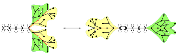
Figure 6: The midline cutting method.

Lemma 3.23.

The map $\operatorname{Tr}$ is a bijection.

Proof.

Given a reduced nearly symmetric extended graph, the position of the cycle indicates the length of the two real segments on the left and right side of the graph that we want to reorganize. In particular, the length of $\alpha$ in step (3) can be recovered from $G$ and hence, knowing the real sequences of $G$, step (3) can be reversed uniquely. Next, we can undo step (2) by flipping the two vertices which are at the inner ends of these two segments. Finally, there is unique way of cutting open the two segments and regluing them as additional tree at the right border vertex to undo step (1). ∎

Lemma 3.24.

Let $G\in\bm{RW}$ be a short graph. Then

$$\varepsilon(\operatorname{Tr}(G))=\begin{cases}-\varepsilon(G)&\text{ if }\operatorname{Tr}(G)\text{ is white-sided},\\ +\varepsilon(G)&\text{ if }\operatorname{Tr}(G)\text{ is black-sided}.\end{cases}$$ (4)

Proof.

Throughout the proof, $\Sigma$ and $\overline{\Sigma}$ will refer to sequences for $G$ and $\operatorname{Tr}(G)$ respectively. By symmetry we may restrict our attention to graphs $G$ with the cycle sitting on the left hand side. Fix a colour $c$ and let $k_{c}$ be the number of transpositions needed to transform $\overline{\Sigma}_{c}$ to $(\overline{\Sigma}_{c}^{{\text{odd}}},\overline{\Sigma}_{c}^{{\text{even}}})$, as in the proof of Lemma 3.17. Set $l_{c}=l(\overline{\Sigma}_{c}^{{\text{even}}})$ and let $n_{c}$ be the number of even vertices of colour $c$ located before the cycle in $\operatorname{Tr}(G)$. In other words, $n_{c}=l(\alpha)$ for the sequence $\alpha$ appearing in step (3). Note that the cyclic shifts applied in step (3) do not affect the number $k_{c}$ and we can express it as

$$k_{c}=\begin{cases}n_{c}&\text{ if }l(\overline{\Sigma}_{c}^{{\text{odd}}})=1,\\ n_{c}+l_{c}&\text{ if }l(\overline{\Sigma}_{c}^{{\text{odd}}})=3.\end{cases}$$ (5)

Let $\delta_{c}$ denote the change of pole disorders from $G$ to $\operatorname{Tr}(G)$ caused by vertices of colour $c$. We have $\delta_{c}=n_{c}$ for $\overline{\Sigma}_{c}^{{\text{odd}}}=(a)$ or $(1,a,1)$ and $\delta_{c}=n_{c}+1$ for $\overline{\Sigma}_{c}^{{\text{odd}}}=(a,b,b)$. Hence the total contribution of the colour $c$ to the sign change can be expressed as

$$\operatorname{dis}(\overline{\Sigma}_{c})-\operatorname{dis}((\Sigma_{c}^{{\text{odd}}},\Sigma_{c}^{{\text{even}}}))+\delta_{c}\equiv\begin{cases}0&\text{ if }l(\overline{\Sigma}_{c}^{{\text{odd}}})=1,\\ l_{c}+1&\text{ if }l(\overline{\Sigma}_{c}^{{\text{odd}}})=3.\end{cases}$$ (6)

Since by assumption $G$ is a white-sided short graph with the cycle located to the left-hand side, we have $\Sigma_{b}=(\Sigma_{b}^{{\text{odd}}},\Sigma_{b}^{{\text{even}}})$ and $\Sigma_{w}=(\Sigma_{w}^{{\text{even}}},\Sigma_{w}^{{\text{odd}}})$. Hence for case $c=w$ we should take into account an extra contribution of $l_{w}$, and thus the sign change for black and white vertices is given in the following table.

	$w$	$b$
$l(\overline{\Sigma}_{c}^{{\text{odd}}})=1$	$(-1)^{l_{w}}$	$+1$
$l(\overline{\Sigma}_{c}^{{\text{odd}}})=3$	$-1$	$(-1)^{l_{b}+1}$

In the case where $\operatorname{Tr}(G)$ is black-sided, we multiply the diagonal entries of the table. Since $l_{w}+l_{b}$ is odd, we obtain the total sign change $+1$. In the case where $\operatorname{Tr}(G)$ is white-sided, we multiply the antidiagonal entries and obtain $-1$. ∎

Proof of Theorem 3.5 for $d$ odd.

Following Corollary 3.21, it is sufficient to prove that $S(\bm{RW})=S(\bm{RB})$. The latter equality follows from Lemmata 3.23 and 3.24. ∎

4 Invariance theorem

In this section we prove Theorem 1.1. We fix $d$ and partitions $\mathbf{\Lambda}=(\Lambda_{1},\ldots,\Lambda_{k})$ of $d$ such that $d=\sum_{i,j}(\Lambda_{j}^{i}-1)$. First note that the number of functions contained in ${\mathcal{S}}({\mathcal{P}},\mathbf{\Lambda})$ only depends on the ordering of the branch points in ${\mathcal{P}}=(b_{1},\dots,b_{k})$ on the real line, not on their exact position. This follows from Theorem 2.4. Hence it remains to prove that the signed count does not change under a permutation of the points in ${\mathcal{P}}$. Based on Section 2 it is slightly more convenient to take the symmetric point of view here: We fix the ordering of points by $b_{1}<\dots<b_{k}$, and instead permute the partitions stored in the sequence $\mathbf{\Lambda}$. Of course, it suffices to prove invariance under the action of the transposition exchanging $\Lambda_{j}$ and $\Lambda_{j+1}$, $j=1,\dots,k-1$.

Let us fix some $j\in\{1,\dots,k-1\}$. The relation to the $bw$-graphs from the previous section is as follows. We rename $\Lambda_{j}=\Lambda_{b}$ and $\Lambda_{j+1}=\Lambda_{w}$. Let $\Gamma$ be a real simple rational dessin of degree $d$ and type $\mathbf{\Lambda}$. We colour the preimages of $b_{j}$ and $b_{j+1}$ in black and white, respectively. Let $E_{bw}:=\varphi^{-1}([b_{j},b_{j+1}])\subset\Gamma$ denote the preimage of the closed segment joining $b_{j}$ and $b_{j+1}$. We need to distinguish two cases. Let us recall from [IZ18, Definition 3.1] that a black and white tree, or $bw$-tree, is a graph as described in Definitions 3.1, except for requiring a tree graph, in exchange for our cycle condition.

1. $E_{bw}$ is a union $T_{1}\cup\ldots\cup T_{r}$ of disjoint $bw$-trees, where some of them are real and others split into pairs of trees that are complex conjugate.

2. $E_{bw}$ is a union $R_{0}\cup T_{1}\cup\ldots\cup T_{r}$ of $bw$-trees $T_{1},\ldots,T_{s}$ as before, together with exactly one real simple $bw$-graph $R_{0}$ (see Figure 7).

Figure 7: An example of a real dessin satisfying condition (b).

We focus on case (b). Case (a) is similar to the situation in [IZ18] and will be treated later. The following definition describes the type of graphs we obtain when we make $b_{j}$ and $b_{j+1}$ “collide” in ${\mathbf{R}}$, or equivalently, collapse the subgraph $E_{bw}\subset\Gamma$. A real polynomial dessin $\tilde{\Gamma}\subset{\mathbf{C}}{\mathbf{P}}^{1}$ is a labelled graph satisfying all the conditions from Definition 2.1 except for condition (c), which we replace by

1. exactly one vertex is labelled by $\infty$, namely $\infty\in{\mathbf{C}}{\mathbf{P}}^{1}$.

Definition 4.1.

A $bw$-enhanced dessin is a real polynomial dessin $\tilde{\Gamma}$ with (ordered) labels $\{1,\dots,j-1,bw,j+2,\dots,\infty\}$ together with the following data:

• A real $bw$-vertex $V_{0}$, together with two partitions $\Pi_{b}(V_{0}),\Pi_{w}(V_{0})$ of $\deg(V_{0})/2+1$.

• Let $\mathcal{V}_{\mathbb{R}}$ be the set of real $bw$-vertices different from $V_{0}$ and let $\mathcal{V}_{+}$ be the set of $bw$-vertices with positive imaginary part. For each vertex $V\in\mathcal{V}_{\mathbb{R}}\cup\mathcal{V}_{+}$, fix two partitions $\Pi_{b}(V),\Pi_{w}(V)$ of $\deg(V)/2$.

From a simple rational dessin $\Gamma$ of type (b) we can construct a $bw$-enhanced real dessin $\tilde{\Gamma}$ as follows. First, we obtain the graph $\tilde{\Gamma}$ by contracting all edges $j\rightarrow j+1$ of $\Gamma$. This means that each component of $E_{bw}=R_{0}\cup T_{1}\cup\ldots\cup T_{r}$ contracts to a point, and we label these points by $bw$. We set $V_{0}$ the vertex of $\tilde{\Gamma}$ obtained from contracting $R_{0}$ and define $\Pi_{b}(V_{0})$ and $\Pi_{w}(V_{0})$ as the partition of degrees of black and white vertices in $R_{0}$, respectively. Similarly, for each vertex $V\in\mathcal{V}_{\mathbb{R}}\cup\mathcal{V}_{+}$, we define $\Pi_{b}(V_{0})$ and $\Pi_{w}(V_{0})$ as the partition of degrees of black and white vertices in $T_{i}$, where $T_{i}$ is the $bw$-tree contracting to $V$. We call $\tilde{\Gamma}$ the contraction of $\Gamma$.

Definition 4.2.

Let $\tilde{\Gamma}$ be a $bw$-enhanced dessin. For any label $j\neq bw,\infty$, we set $\Sigma_{j}$ to the sequence of degrees of real vertices labelled by $j$, ordered from left to right. We denote by $\tilde{\Sigma}_{w}$ and $\tilde{\Sigma}_{b}$ the sequences of partitions $\Pi_{w}(V)$ and $\Pi_{b}(V)$, respectively, running through the real $bw$-vertices (from left to right), except for $V_{0}$, for which we use the partitions $(\Pi_{w}(V),1)$ and $(\Pi_{b}(V),1)$. A disorder of $\tilde{\Sigma}_{w}$ or $\tilde{\Sigma}_{b}$ is a pair of entries $\Pi_{w}^{k}(V)>\Pi_{w}^{k^{\prime}}(V^{\prime})$ or $\Pi_{b}^{k}(V)>\Pi_{b}^{k^{\prime}}(V^{\prime})$, respectively, with $V<V^{\prime}$. Clearly, multiple entries of a partition are counted multiple times here. We set

$$\operatorname{dis}(\tilde{\Gamma}):=\operatorname{dis}(\tilde{\Sigma}_{w})+\operatorname{dis}(\tilde{\Sigma}_{b})+\sum_{j\neq bw,\infty}\operatorname{dis}(\Sigma_{j}),\quad\quad\quad\quad\varepsilon(\tilde{\Gamma}):=(-1)^{\operatorname{dis}(\tilde{\Gamma})}.$$

Recall from [IZ18] that the sign $\varepsilon(T)$ of a real $bw$-tree is $(-1)^{\operatorname{dis}(\Sigma_{w})+\operatorname{dis}(\Sigma_{b})}$.

Lemma 4.3.

If a $bw$-enhanced dessin $\tilde{\Gamma}$ is the contraction of a dessin $\Gamma$, then

$$\varepsilon(\Gamma)=\varepsilon(\tilde{\Gamma})\cdot\varepsilon(R_{0})\cdot\prod_{T}\varepsilon(T),$$

where the product is taken over the real trees in $E_{bw}$.

Proof.

The right hand side of the formula takes care of all disorders contributing to $\varepsilon(\Gamma)$ except for the ones involving a vertex in the interior of the (topological) edge $E$ of $\Gamma$ containing $p$. Note that for each label $i\in\{j+2,\dots k,\infty,1,\dots,j-1\}$ there is exactly one vertex labelled by $i$ in the interior of $E$, and all these vertices have valance to $2$. Hence such disorders appear in pairs: Any higher-degree real vertex to the left of $p$ produces exactly one level and one pole disorder. This proves the formula. ∎

Let $\tilde{\Gamma}$ be a $bw$-enhanced dessin. For any real $bw$-vertex $V$, we define the colour $c(V)$ to be white if the real edge to the right of $V$ is of type $bw\to j+2$. Otherwise we set $c(V)$ to be black. We denote by $\mathcal{R}_{0}$ the set of $c(V)$-sided real simple $bw$-graphs of type $\Pi_{b}(V_{0}),\Pi_{w}(V_{0})$. For any $V\in\mathcal{V}_{\mathbb{R}}$ we denote by $\mathcal{T}_{V}$ the set of $c(V)$-sided real $bw$-trees of type $\Pi_{b}(V),\Pi_{w}(V)$. For any $V\in\mathcal{V}_{+}$ we denote by $\mathcal{T}_{V}$ the set of (non-real) $bw$-trees of type $\Pi_{b}(V),\Pi_{w}(V)$ with one marked half-edge emanating from a white vertex.

For any $V\in\mathcal{V}_{+}$, let us mark an adjacent edge _V of type $bw\to j+2$. Let $\mathcal{M}$ denote the set of increasing real simple dessins $\Gamma$ that contract to $\tilde{\Gamma}$. Then we can define a map

$$F:\mathcal{M} \to\mathcal{R}_{0}\times\prod_{V\in\mathcal{V}_{\mathbb{R}}\cup\mathcal{V}_{+}}\mathcal{T}_{V},$$

$$\Gamma \mapsto(R_{0},T_{V}:V\in\mathcal{V}_{\mathbb{R}}\cup\mathcal{V}_{+}),$$

where $R_{0}$ and $T_{V}$ denote the components of $E_{bw}$ contracting to $V_{0}$ and $V$, respectively. For $V\in\mathcal{V}_{+}$, we additionally mark the first half-edge in $T_{V}$ touching $e_{V}$, counted in clockwise direction.

Lemma 4.4.

The map $F$ is a bijection.

Proof.

We can easily describe the inverse map. Given $(R_{0},\leavevmode\nobreak\ T_{V}:V\in\mathcal{V}_{\mathbb{R}}\cup\mathcal{V}_{+})$, we insert $R_{0}$ and $T_{V}$ into a small disc removed around $V_{0}$ and $V\in\tilde{\Gamma}$, respectively, as described in [IZ18, Proof of Lemma 4.6]. Additionally, we fill the “hole” bounded by the cycle in $R_{0}$ as follows. Let $D\subset{\mathbf{C}}$ denote the unique affine real polynomial dessin of degree $1$ labelled by $-\infty\to j+2\to\dots\to k\to\infty\to 1\to\dots\to j-1\to+\infty$. We glue $D$ into the hole such that the edge $-\infty\to j+2$ is attached to the white vertex in the boundary (see Figure 8). In this way we obtain real simple rational dessin $\Gamma$ such that $F(\Gamma)$ is equal to the given data. ∎

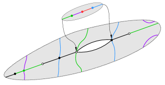
Figure 8: Filling the “hole” of $R_{0}$.

Corollary 4.5.

With the notation used in Lemma 4.4, we have

$$S(\mathcal{M})=\varepsilon(\tilde{\Gamma})\;S(\mathcal{R}_{0})\prod_{V\in\mathcal{V}_{\mathbb{R}}}S(\mathcal{T}_{V})\prod_{V\in\mathcal{V}_{+}}|\mathcal{T}_{V}|.$$

Proof.

Follows from Lemma 4.3 and Lemma 4.4. ∎

Proof of Theorem 1.1.

Since transpositions of the form $(j,j+1)$ generate the symmetric group, it is enough to prove $S({\mathcal{S}}({\mathcal{P}},\mathbf{\Lambda}))=S({\mathcal{S}}({\mathcal{P}},\mathbf{\Lambda}^{\prime}))$, where $\mathbf{\Lambda}^{\prime}$ is the sequence of partitions with $\Lambda_{j}$ and $\Lambda_{j+1}$ swapped. Let ${\mathcal{S}}^{\text{\ref{bw1}}}({\mathcal{P}},\mathbf{\Lambda})$ and ${\mathcal{S}}^{\text{\ref{bw2}}}({\mathcal{P}},\mathbf{\Lambda})$ be the subsets of functions/dessins of type (a) and (b), respectively. Then $S({\mathcal{S}}^{\text{\ref{bw1}}}({\mathcal{P}},\mathbf{\Lambda}))=S({\mathcal{S}}^{\text{\ref{bw1}}}({\mathcal{P}},\mathbf{\Lambda}^{\prime}))$ follows, after some straightforward adaptation to our case, from [IZ18, Lemma 4.8]. It remains to show $S({\mathcal{S}}^{\text{\ref{bw2}}}({\mathcal{P}},\mathbf{\Lambda}))=S({\mathcal{S}}^{\text{\ref{bw2}}}({\mathcal{P}},\mathbf{\Lambda}^{\prime}))$. We can prove this for each contraction separately. More precisely, let $\tilde{\Gamma},\tilde{\Gamma}^{\prime}$ be a pair of $bw$-enhanced dessins obtained from each other by flipping the partitions $\Pi_{b}(V),\Pi_{w}(V)$ for any $bw$-vertex $V$. Let $\mathcal{M}$ and $\mathcal{M}^{\prime}$ be the sets of dessins of type $\mathbf{\Lambda}$ and $\mathbf{\Lambda}^{\prime}$ that contract to $\tilde{\Gamma}$ and $\tilde{\Gamma}^{\prime}$, respectively. We show $S(\mathcal{M})=S(\mathcal{M}^{\prime})$ using Corollary 4.5. Indeed, the invariance of the various factors follows for $\varepsilon(\tilde{\Gamma})$ by definition, for $S(\mathcal{R}_{0})$ by Theorem 3.5, for $S(\mathcal{T}_{V})$ by [IZ18, Theorem 9], and for $|\mathcal{T}_{V}|$ by switching the colours of the vertices. Note that in the last case, the number of half-edges adjacent to a white and black vertex, respectively, is equal and hence the number of possible markings does not change. ∎

Remark 4.6.

Despite the combinatorial nature of the presented proof of Theorem 1.1 it is instructive to also get a geometric picture of the degeneration when $b_{j}$ and $b_{j+1}$ collide. While in our description the two discs adjacent to $p$ just collapse to $V_{0}$ in $\tilde{\Gamma}$, the limit of this degeneration in $\overline{{\mathcal{M}}}_{0,0}({\mathbf{C}}{\mathbf{P}}^{1},d)$ is a ramified cover with reducible source curve. The “bubbling” produces a source curve with two components (see Figure 9). The main component is described by $\tilde{\Gamma}$ and is mapped to ${\mathbf{C}}{\mathbf{P}}^{1}$ by a polynomial map of degree $d-1$. The bubble corresponds to the two discs adjacent to $p$ and is mapped isomorphically to ${\mathbf{C}}{\mathbf{P}}^{1}$. The vertex $V_{0}$ is the node connecting the two spheres. This phenomenon does not occur in the polynomial case of [IZ18]. What keeps the situation under control for simple rational functions is the fact that the degree $1$ map on the bubble is essentially unique and hence can be discarded from the combinatorial data.

Figure 9: The bubbling of a dessin into a reducible dessin of degree $(d-1,1)$.

5 Vanishing Statements

This section is devoted to proving the vanishing statements contained in Theorem 1.2 or, in other words, the only if part. Let $\bm{\lambda}:=(\lambda_{1},\ldots,\lambda_{k})$ be a sequence of reduced partitions as in the introduction.

Proposition 5.1 (First part of non-vanishing for all degrees).

If a partition $\lambda_{j}$ has more than one odd number appearing an odd number of times or more than one even number appearing an odd number of times, then $F_{\bm{\lambda}}^{\text{odd}}(q)=0$ and $F_{\bm{\lambda}}^{\text{even}}(q)=0$.

Proof.

Fix $a\neq b$ of the same parity which both appear an odd number of times in $\lambda_{j}$. Then for any dessin $\Gamma$ there is an odd number of real vertices of label $j$ and degree $2a+2$ and $2b+2$, respectively. Let $v_{1}<\dots<v_{2m}$ be the totality of such vertices. We want to invert the order of appearance of these vertices by applying a flip operation of the form

$$\operatorname{Flip}^{v_{1}}_{v_{2m}}\circ\dots\circ\operatorname{Flip}^{v_{m}}_{v_{m+1}}.$$ (7)

where $\operatorname{Flip}^{v}_{w}$ is the following adaptation of Definition 3.8.

1. If $v$ and $w$ have the same degree, we do nothing.

2. If $v$ and $w$ have degree $2a+2$ and $2b+2$, respectively, and $a>b$, we set $F(v):=(T_{1},\dots,T_{2(a-b)})$ to be the sequence of pairs of trees growing at $v$ and closest to the negative direction of ${\mathbf{R}}$. If $a<b$, we proceed symmetrically.

3. The real segments near $v,w$ can be of the following types.

   $$a,b\text{ even:} j-1\rightarrow j\rightarrow j+1 j+1\rightarrow j\rightarrow j-1$$ or

   $$a,b\text{ odd:} j-1\rightarrow j\rightarrow j-1 j+1\rightarrow j\rightarrow j+1$$ or

   If $v$ and $w$ are of the same type, we remove $F(v)$ from $v$ and glue it to $w$ (say, closest to the negative direction of ${\mathbf{R}}$, but not in the interior of the cycle, if present). If the vertices are of opposite type, we glue back the inverted sequence $F(v)^{-1}$ instead. In this way, we ensure that the pattern of increasing and decreasing edges alternates when going around $w$, as required.

In summary, we see that operation (7) defines an involution on the set of dessins which inverts the order of appearance of the vertices $v_{1},\dots,v_{2m}$. It is shown in [IZ18, Page 37] that this operation flips the sign of a dessin. Note that cited argument can be applied to our situation since the number of pole disorders is not affected by (7). Hence the statement follows. ∎

Proposition 5.2 (non-vanishing for odd degrees).

Consider a sequence of partitions $\bm{\lambda}$ which does not satisfy the conditions of Proposition 5.1. If there is an odd number of partitions $\lambda_{j}$ having an even element appearing an odd number of times, then

$$F^{{\text{odd}}}_{\bm{\lambda}}(q)=0.$$

Proof.

For $d$ odd the operation $\varphi(z)\mapsto\tilde{\varphi}(z)=\varphi(-z)$ produces an increasing function again and hence defines an involution on ${\mathcal{S}}({\mathcal{P}},\mathbf{\Lambda})$. Let $\Sigma=\Sigma_{b_{j}}$ the ramification sequence of a critical value as in Definition 1.5. Then the corresponding sequence for $\tilde{\varphi}$ is given by $\Sigma^{-1}$, the inverted sequence. One easily checks

$$\operatorname{dis}(\Sigma)+\operatorname{dis}(\Sigma^{-1})\equiv_{2}c(\Sigma),$$

where

$$c(\Sigma):=\sharp\{\text{pairs of numbers}\leavevmode\nobreak\ m,n\leavevmode\nobreak\ \text{in}\leavevmode\nobreak\ \Sigma\leavevmode\nobreak\ \text{such that}\leavevmode\nobreak\ m\neq n\}.$$

Recall that $\Sigma$ includes a $1$ coming from the simple pole, so the sum of its entries is even. Now, if $\lambda_{i}$ contains an even number $a$ an odd number of times, then $\Sigma$ contains two or three elements appearing an odd number of times ($1$, $a+1$, and possibly an even entry), and hence $c(\Sigma)$ is odd. If, on the other hand, $\lambda_{j}$ does not contain an even element an odd number of times, then $\Sigma$ contains zero or one elements appearing an odd number of times and hence $c(\Sigma)$ is even. The result then follows by the previous formula. ∎

Remark 5.3.

For $d$ even, we could instead try to use the transformation $\varphi(z)\mapsto-\varphi(-z)$, which provides a bijection between ${\mathcal{S}}({\mathcal{P}},\mathbf{\Lambda})$ and ${\mathcal{S}}(-{\mathcal{P}},\mathbf{\Lambda})$. The same argument as above shows that $F^{{\text{even}}}_{\bm{\lambda}}(q)=0$ if there is an odd number of partitions $\lambda_{j}$ with an odd entry appearing an odd number of times. But note that such entries correspond to local extrema of $\varphi$. Hence the number is even.

6 Broken alternations

Definition 6.1.

Let $a\in\operatorname{Sym}(n)$ be a permutation on $n$ elements, $i\mapsto a_{i}$. We call $a$ an (ordinary) alternation if $a_{n}<a_{n-1}>a_{n-2}<a_{n-3}>\dots\lessgtr a_{1}$. The permutation $a$ is said to be a broken alternation if it is an alternation except for exactly one index $i\in\{1,\dots,n-1\}$, where $a_{i},a_{i+1}$ is increasing if it should be decreasing, or the opposite. In this case, $i$ is called the break of $a$, and we write $(a_{1}\dots a_{i}|a_{i+1}\dots a_{n})$. We denote by $A_{n}$, $B_{n}$ and $B_{n}^{j}$ the number of ordinary alternations, broken alternations, broken alternations with $a_{j}=n$, respectively.

It is clear that we have $A_{1}=A_{2}=B_{2}=1$, $B_{1}=0$, and $B_{n}=B_{n}^{1}+\dots+B_{n}^{n}$.

Proposition 6.2.

There is a one-to-one correspondence between broken alternations of $n$ elements and real simple rational dessins of degree $n$ and type $\mathbf{\Lambda}=(\Lambda_{1},\dots,\Lambda_{n})$, $\Lambda_{1}=\dots=\Lambda_{n}=(21\dots 1)$. Moreover, the sign of any such real simple rational dessin is equal to $-1$ to the power of $\left\lfloor n/2\right\rfloor$.

Remark 6.3.

The exact same relation holds between ordinary alternations and real polynomial dessins, see [IZ18, Example 1.5]. We refer to Figure 10 for examples.

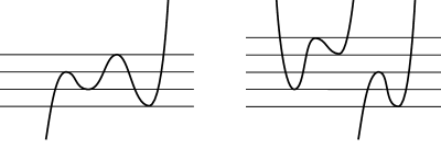
Figure 10: To the left, a polynomial representing the ordinary alternation $a=(3241)$. To the right, a simple rational function representing the broken alternation $a=(254|31)$.

Proof of Proposition 6.2.

Given a real simple rational dessins of type $\mathbf{\Lambda}$, the sequence of labels of the real vertices of degree greater than $2$, ordered from left to right, produces a broken alternation of length $n$. The break corresponds to passing through the simple pole $p$. Vice versa, given a broken alternation $a$, we can construct a dessin as follows. We place $4$-valent vertices on $\mathbb{R}$ with labels as described in $a$. We put a $2$-valent vertex with label $\infty$ on the segment between the vertices corresponding to the break of $a$. We glue the imaginary ends of the graph to infinity, except for the ends to the left and right of $p$, which we glue pairwise to obtain a pair of cycles. Finally we insert $2$-valent vertices in the unique way to complete the graph to a dessin. The sign is deduced by noting that an real simple rational function of type $\Lambda_{n}$ has exactly $\lfloor n/2\rfloor$ local maxima, and each local maxima contributes by a factor of $-1$. ∎

We can easily derive recursive formulas for the numbers $B_{n},B_{n}^{j}$ similar to those for $A_{n}$. In accordance with Proposition 6.2, we set $B_{0}=0$, $A_{0}=1$.

Proposition 6.4.

For $n\geq 2$ we have

$$B_{n}^{j}=\begin{cases}\binom{n-1}{j-1}\cdot(B_{j-1}A_{n-j}+A_{j-1}B_{n-j})&\text{if $n+j$ odd,}\\ A_{n-1}&\text{if $j=n$ or $n$ odd, $j=1$,}\\ 0&\text{otherwise.}\end{cases}$$

Proof.

By our conventions, the pattern for ordinary alternations is $a_{j-1}<a_{j}>a_{j+1}$ for $n+j$ odd, and $a_{j-1}>a_{j}<a_{j+1}$ otherwise. In a broken alteration, we can flip at most one of these inequalities. Hence, if $a$ is a broken alternation with $a_{j}=n$, we have the following cases. If $n+j$ is even, it is of the form $a=(n|a^{\prime})$ or $a=(\overline{a^{\prime}}|n)$, where $a^{\prime}$ is an ordinary alternation of length $n-1$ and $\overline{a^{\prime}}$ is defined by $\overline{a^{\prime}_{i}}=n-a^{\prime}_{i}$. The map $a\mapsto a^{\prime}$ is obviously a bijection, which settles the second and third case. If $n+j$ is odd, the break of $a$ is different from $j-1$ and $j$. Hence $a$ is of the form $(a^{\prime}na^{\prime\prime})$, where either $a^{\prime}$ is ordinary and $a^{\prime\prime}$ is broken, or vice versa. To be precise, this is true after using the unique ordered relabelling of the values of $a^{\prime},a^{\prime\prime}$ to $\{1,\dots,j-1\}$ and $\{1,\dots,n-j\}$, respectively. On other hand, a (relabelled) pair $(a^{\prime},a^{\prime\prime})$ occurs exactly $\binom{n-1}{j-1}$ times in these constructions, since this is the number of ordered maps $\{1,\dots,j-1\}\to\{1,\dots,n-1\}$ (or, equivalently, $\{1,\dots,n-j\}\to\{1,\dots,n-1\}$). ∎

The first few values of $B_{n}$ are given in the following table.

$$\begin{array}[]{c|ccccccccccccc}n&1&2&3&4&5&6&7&8&9&10&11&12\\ \hline\cr B_{n}&0&1&2&7&26&117&594&3407&21682&151853&1160026&9600567\end{array}$$

It seems that the sequence has not appeared in the literature before (cf. [Sta10]) and is not recorded on OEIS.

We can turn the recursive relations into differential equations for generating series. Since it is more convenient to do this for odd and even indices separately, we define for the ordinary alternations

$$f(q):=\sum_{k=0}^{\infty}(-1)^{k}\frac{A_{2k+1}}{(2k+1)!}q^{2k+1},\quad g(q):=\sum_{k=0}^{\infty}(-1)^{k}\frac{A_{2k}}{(2k)!}q^{2k},$$

and for the broken alternations

$$u(q):=\sum_{k=0}^{\infty}(-1)^{k}\frac{B_{2k+1}}{(2k+1)!}q^{2k+1},\quad v(q):=\sum_{k=0}^{\infty}(-1)^{k}\frac{B_{2k}}{(2k)!}q^{2k}.$$

Lemma 6.5.

The power series $f,g,u,v$ satisfy the following differential equations.

$$u^{\prime} =2(g-fu-1),$$ (8)

$$v^{\prime} =-(f+fv+gu).$$ (9)

Proof.

From Proposition 6.4, for $k\geq 1$ we have

$$B_{2k+1} =2A_{2k}+\sum_{j=1}^{k}\binom{2k}{2j-1}\cdot\left(B_{2j-1}A_{2k+1-2j}+A_{2j-1}B_{2k+1-2j}\right)$$ (10)

$$=2\left(A_{2k}+\sum_{j=1}^{k}\binom{2k}{2j-1}\cdot B_{2j-1}A_{2k-(2j-1)}\right).$$ (11)

which proves the first equation for all non-constant terms. For the constant term, we note that by our conventions $B_{1}=2(A_{0}-0-1)=0$. Again by Proposition 6.4, for $k\geq 1$ we have

$$B_{2k} =A_{2k-1}+\sum_{j=0}^{k-1}\binom{2k-1}{2j}\cdot\left(B_{2j}A_{2k-2j-1}+A_{2j}B_{2k-2j-1}\right),$$ (12)

$$=A_{2k-1}+\sum_{j=0}^{2k-1}\binom{2k-1}{j}\cdot B_{j}A_{2k-1-j},$$ (13)

The sum in (13) corresponds to the anti-symmetric part of $(f+g)(u+v)$ which is $fv+gu$. Moreover, because of the antisymmetry of the second equation, no constant term appears, which completes the proof. ∎

We can solve these differential equations explicitly. Recall the 19th century result [And81] (see also [Sta10]) that

$$f(q)=\tanh(q)\quad\text{and}\quad g(q)=\operatorname{sech}(q).$$

Corollary 6.6.

The generating series $u$ and $v$ can be expressed as

$$u(q) =-f-q+qf^{2}+2fg,$$ (14)

$$v(q) =1-2f^{2}-g+qfg.$$ (15)

Proof.

The given descriptions for $u$ and $v$ are the unique solutions to the equations (8) and (9) with initial conditions $u(0)=v(0)=0$. ∎

7 Polynomiality

Keeping the notations from the introduction, we want to prove the following result.

Theorem 7.1.

For any sequence of reduced partitions ${\bm{\lambda}}$, the generating series

$$F^{odd}_{{\bm{\lambda}}}(q)\quad\text{and}\quad F^{even}_{{\bm{\lambda}}}(q)$$

are polynomials in $q$, $f(q)$ and $g(q)$ with rational coefficients.

Based on the invariance theorem 1.1, we fix points $b_{1}<b_{2}<\dots<b_{m+k}$ and consider real simple rational functions with simple branch points $b_{1},\ldots,b_{m}$ and reduced ramification profile $\lambda_{1},\ldots,\lambda_{k}$ at the branch points $b_{m+1},\dots,b_{m+k}$. We choose an additional point $b_{m}<\alpha<b_{m+1}$.

Let $\varphi$ be such a function and $\Gamma$ be the associated affine dessin of $\varphi$. We set $B^{\prime}$ to be the union of connected components of $\varphi^{-1}([\alpha,\infty))$ which contain a critical point of $\varphi$ (see Figure 11). We also include the components of $\varphi^{-1}([\alpha,\infty))$ to the left and right which contain unbounded pieces of $\mathbb{R}$. Since the left one only exists if $d$ is odd, this is just a convenient way of storing the parity of $d$ in $B^{\prime}$.

Definition 7.2.

A connected component $C$ of ${\mathbf{R}}\setminus B^{\prime}$ is a chain of $\Gamma$. Each point in the inverse image of $\alpha$ is labelled by $\blacksquare$, and is called an $\alpha$-vertex. We order the chains from left to right as $C_{1},\dots,C_{l}$. The special chain $C_{\text{s}},\text{s}\in\{1,\dots,l\}$ is chain containing the simple pole $p$. The tuple $B_{\Gamma}:=(B^{\prime},\text{s})$ is called the base of $\Gamma$.

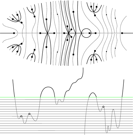
Figure 11: A base $B$ of type (a), represented as a union of thick lines. Here, $l=4$, $\text{s}=3$ and $(c_{1},c_{2},c_{3},c_{4})=(2,0,0,1)$. The black squares are the $\alpha$-vertices. The dotted lines represent the inverse image of $(-\infty,\alpha)$ for a dessin $\Gamma$ with $B_{\Gamma}=B$.

Let $q_{1},q_{2}$ denote the closest critical points before and after the simple pole $p$. We need to distinguish three cases (see Figures 11, 13, and 14 for examples):

1. $\varphi(q_{1}),\varphi(q_{2})>\alpha$,

2. $\varphi(q_{1})>\alpha>\varphi(q_{2})$ or $\varphi(q_{2})>\alpha>\varphi(q_{1})$,

3. $\varphi(q_{1}),\varphi(q_{2})<\alpha$.

The three cases can be distinguished in terms of the base as follows.

1. The base $B_{\Gamma}$ contains a cycle.

2. The base $B_{\Gamma}$ contains no cycle, but a bounded open end (with the simple pole $p$ as endpoint).

3. Otherwise.

Remark 7.3.

To motivate the following definition, let us make a few simple observations. Let $C_{1},\dots,C_{l}$ be the sequence of chains, the order of which is according to the orientation of $\mathbb{R}$. Let $r_{i}$ denote the number of critical points occurring in $C_{i}$. Then the parity of $r_{i}$ is given by

$$r_{i}\equiv_{2}\begin{cases}d&i=1,\\ 1&i>1,\end{cases}$$ (16)

except for the following cases:

$$r_{\text{s}}\equiv_{2}\begin{cases}d-1&\text{s}=1,\text{and either type \ref{case1} or \ref{case2}},\\ 0&\text{s}>1,\text{and either type \ref{case1} or \ref{case2}}.\end{cases}$$ (17)

Moreover, we have

$$r_{\text{s}}=0\quad\quad\text{ if }B\text{ is of type \ref{case1}}.$$ (18)

In the following, we fix a base $B=(B^{\prime},\text{s})$ of type (a), (b) or (c) and chains $C_{1},\dots,C_{l}$. Note that for type (a) and (b), the special index s is uniquely determined by $B^{\prime}$, while for type (c) any $\text{s}\in\{1,\dots,l\}$ can occur. Let $Z_{+}$ be a connected component of $B$ which is contained in $\{z:\Im(z)>0\}\subset{\mathbf{C}}$. It has a unique $\alpha$-vertex which can be connected in ${\mathbf{C}}\setminus B$ to a unique chain $C_{i}$. We say $Z_{+}$ is adjacent to $C_{i}$ and denote by $c_{i}$ the number of such $Z_{+}$ (see Figure 11).

Definition 7.4.

A chain data set for a base $B$ consists of a tuple $(I_{i},a_{i},M_{i})_{i\in\{1,\dots,l\}}$ with the following properties.

1. The sets $I_{i}$ form a disjoint union $I_{1}\sqcup\dots\sqcup I_{l}=\{1,\dots,m\}$ and the numbers $r_{i}:=|I_{i}|$ satisfy equations (16), (17) and (18).

2. For any $i\in\{1,\dots,\hat{\text{s}},\dots,l\}$, $a_{i}$ is an ordinary alternation $a_{i}$ of length $r_{i}$. Additionally, $a_{\text{s}}$ is an ordinary or broken alternation of length $r_{\text{s}}$ if type is (b) or (c). For type (a), we set $a_{\text{s}}=\emptyset$.

3. We set $m_{i}:=\left\lfloor r_{i}/2\right\rfloor$ for $i\neq\text{s}$. We set $m_{\text{s}}:=\left\lfloor r_{\text{s}}/2\right\rfloor-1$, except for the case type (b), $d$ even, and $\text{s}=1$, in which we set $m_{\text{s}}:=\left\lfloor r_{\text{s}}/2\right\rfloor$. Then the last ingredient is a choice of subsets $M_{i}\subset\{1,\dots,m_{i}\}$ of size $c_{i}$.

Proposition 7.5.

Fix a base $B$ as above. Then the set of dessins $\Gamma$ with $B=B_{\Gamma}$ is in one-to-one correspondence with the set of chain data sets for $B$.

Proof.

We first associate a chain data set to each $\Gamma$. Fix $i\in\{1,\dots,l\}$. We define $I_{i}$ such that $j\in I_{i}$ if and only if the simple critical point with value $b_{j}$ is contained in $C_{i}$. After reparametrising $I_{i}$ by $\{1,\dots,r_{i}\}$ keeping the ordering, the order of appearance of the critical points in $C_{i}$ defines a permutation of $\{1,\dots,r_{i}\}$. If the type is (b), $i=\text{s}$, and the simple pole is located on the right hand side of $C_{\text{s}}$, we additionally compose with the permutation with $x\mapsto r_{\text{s}}+1-x$. The result is used as $a_{i}$. Note that $m_{i}$ appearing in Definition 7.4 is equal to the number of maxima in $C_{i}$ for $i\neq\text{s}$, and equal to the number of maxima minus one if $i=\text{s}$ and the type is (b) or (c). In this case, there is a unique maximum in $C_{\text{s}}$ which is closest to the simple pole $p$ (see Figure 12). After removing this maximum, the remaining maxima can be ordered increasingly and labelled by $\{1,\dots,m_{i}\}$. Let $Z_{+}$ be a connected component of $B$, as before, adjacent to $C_{i}$. Since $\Gamma$ is connected, there is path connecting $Z_{+}$ and ${\mathbf{R}}$. It is easy to see that this path is unique, its starting point is a $\alpha$-vertex of $Z_{+}$ and its endpoint is a maximum of $C_{i}$. Varying $Z_{+}$, this construction distinguishes $c_{i}$ maxima of $C_{i}$, whose labels we collect in $M_{i}\subset\{1,\dots,m_{i}\}$. By the properties of $\Gamma$ it is clear that we constructed a well-defined chain data set for $B$.

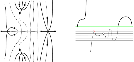
Figure 12: The special chain of a base of type (b). The ticked maximum cannot be marked in $M_{\text{s}}$.

We proceed to show the existence of the inverse map. Assume we are given a chain data set for $B$. Fix some $i\in\{1,\dots,l\}$. Using the bijections in Proposition 6.2 and [IZ18, Example 1.5], we can associate to $a_{i}$ a unique (affine) real dessin $D_{i}$ with labels $1\to\dots\to r_{i}$. Reversing the relabelling from above, we can rename the labels by elements of $I_{i}$. We complete this to a labelling of type $-\infty\to 1\to\dots\to m\to+\infty$ by adding two-valent vertices as necessary. The next step is to glue the $D_{i}$ into ${\mathbf{C}}$ such that their real parts go to $C_{i}$ keeping the orientation. We do this such that ${\mathbf{R}}$ is fully covered by $B$ and the $D_{i}$ (in type (a) and (b), we have to throw in by hand the point $p$ which closes up the open bounded end of $B$). The next step is to connect some non-real ends of $D_{i}$ to $B$. Of course, it suffices to describe the construction in the upper half plane, and then copy it symmetrically. We start with type (b) and $i=\text{s}$. In this case there is a unique maximum in $D_{\text{s}}$ closest to $p$, and an end of $D_{\text{s}}$ emanating from it. There is a unique $\alpha$-vertex contained in the connected component of $B$ adjacent to $p$ and to which this end of $D_{i}$ can be glued. We connect them. Among the $m_{i}$ maxima of $D_{i}$ which are not “adjacent” to $p$, we select the subset of size $c_{i}$ corresponding to $M_{i}$. We consider the $c_{i}$ ends of $D_{i}$ which emanate from the these maxima. There is a unique way (up to homeomorphism) to glue these ends to $\alpha$-vertices of the connected components of $B$ adjacent to $C_{i}$ without producing extra intersections. Again, we connect them like this. We now complete the dessins as follows. Each end of $D_{i}$ of type $m\to\infty$ not yet glued to a $\alpha$-vertex is replaced by a sequence of edges $m\to m+1\to\dots m+k\to+\infty$. This includes, in type (c), the end adjacent to the simple pole in $D_{\text{s}}$. Finally, all non-real ends $-\infty\to 1$ and $m+k\to+\infty$ are extended to infinity to obtain an honest affine dessin $\Gamma$. It is clear that this is indeed the inverse map we are looking for. ∎

Using this Proposition, we can explicitly describe the generating series of $S$-numbers for a given base $B$. Similar to dessins, we consider two bases isomorphic, denoted by $B_{1}\cong B_{2}$, if they can be identified under a $\operatorname{conj}$-equivariant homeomorphism of ${\mathbf{C}}$ that is orientation-preserving on ${\mathbf{R}}$.

Definition 7.6.

Given a base $B=(B^{\prime},\text{s})$, we denote by ${\mathcal{S}}_{B}({\mathcal{P}},\mathbf{\Lambda})$ the set of real simple rational dessins $\Gamma$ with $B_{\Gamma}\cong B$. We set $S_{B}({\bm{\lambda}},m):=S({\mathcal{S}}_{B}({\mathcal{P}},\mathbf{\Lambda}))$ and

$$F_{B}:=\sum_{m\geq 0}S_{B}({\bm{\lambda}},m)\frac{q^{m}}{m!}.$$

Remark 7.7.

Clearly, after fixing the parity of $d$ and ${\bm{\lambda}}$, there is only a finite collection of isomorphism classes of bases that occur as $B_{\Gamma}$. Hence we can express $F^{\text{odd}}_{\bm{\lambda}}$ and $F^{\text{even}}_{\bm{\lambda}}$ as finite sums

$$F^{\text{odd}}_{\bm{\lambda}}=\sum_{B}F_{B}\quad\text{ and }\quad F^{\text{even}}_{\bm{\lambda}}=\sum_{B}F_{B}.$$

Definition 7.8.

Let $B$ be a base and let $\Sigma_{j}$ be the sequence of degrees of real vertices of $B$ contributing to $\lambda_{j}$ (i.e., the vertices with label $m+j$), with an extra $1$ inserted at the position of $C_{\text{s}}$ only if $B$ is of type (a) or (b). The sign of a base $B$ is

$$\varepsilon(B):=(-1)^{\operatorname{dis}\Sigma_{1}+\dots+\operatorname{dis}\Sigma_{k}}.$$

Remark 7.9.

In case (c), two consecutive $1$’s should be inserted, one for the simple pole $p$, and one for the $2$-valent vertex on the segment in $\varphi^{-1}([\alpha,\infty))$ adjacent to $p$, which is not part of $B$. In the definition, equivalently, we do not insert anything.

We denote the differential operator $D=q\frac{d}{dq}$. We introduce the following functions

$$f_{c} =\frac{1}{2^{c}c!}(D-1)(D-3)\cdots(D-2c+1)f,$$

$$g_{c} =\frac{1}{2^{c}c!}D(D-2)\cdots(D-2c+2)g,$$

$$\tilde{g}_{c} =\frac{1}{2^{c}c!}(D-2)(D-4)\cdots(D-2c)g,$$

$$u_{c} =\frac{1}{2^{c}c!}(D-3)(D-5)\cdots(D-2c-1)u,$$

$$v_{c} =\frac{1}{2^{c}c!}(D-2)(D-4)\cdots(D-2c)v.$$

Theorem 7.10.

Fix a base $B$ and set $\varepsilon=\varepsilon(B)$. Then, depending on the different cases, the generating series $F_{B}$ can be written as in the following table.

$$\begin{array}[]{c|c|c|c|c}F_{B}&\text{type \ref{case1}}&&\text{type \ref{case2}}&\text{type \ref{case3}}\\ \cline{1-2}\cr\cline{4-5}\cr d\text{ odd}&\displaystyle\varepsilon\,\prod_{\begin{subarray}{c}i=1\\ i\neq\text{s}\end{subarray}}^{l}f_{\displaystyle c_{i}}&&\displaystyle\varepsilon\,\tilde{g}_{\displaystyle c_{\text{s}}}\,\prod_{\begin{subarray}{c}i=1\\ i\neq\text{s}\end{subarray}}^{l}f_{\displaystyle c_{i}}&\displaystyle\varepsilon\,u_{\displaystyle c_{s}}\,\prod_{\begin{subarray}{c}i=1\\ i\neq\text{s}\end{subarray}}^{l}f_{\displaystyle c_{i}}\\[5.0pt] \hline\cr\hbox{\multirowsetup d \text{ even}}&\hbox{\multirowsetup $\displaystyle\varepsilon\,g_{\displaystyle c_{1}}\,\prod_{\begin{subarray}{c}i=1\\ i\neq\text{s}\end{subarray}}^{l}f_{\displaystyle c_{i}}$}&\text{s}=1&\displaystyle-\varepsilon\,f_{\displaystyle c_{1}}\,\prod_{i=2}^{l}f_{\displaystyle c_{i}}&\displaystyle\varepsilon\,v_{\displaystyle c_{1}}\,\prod_{i=2}^{l}f_{\displaystyle c_{i}}\\ \cline{3-5}\cr&&\text{s}\neq 1&\displaystyle\varepsilon\,g_{\displaystyle c_{1}}\,\tilde{g}_{\displaystyle c_{\text{s}}}\prod_{\begin{subarray}{c}i=2\\ i\neq\text{s}\end{subarray}}^{l}f_{\displaystyle c_{i}}&\displaystyle\varepsilon\,g_{\displaystyle c_{1}}\,u_{\displaystyle c_{\text{s}}}\,\prod_{\begin{subarray}{c}i=2\\ i\neq\text{s}\end{subarray}}^{l}f_{\displaystyle c_{i}}\\ \hline\cr\end{array}$$

Proof.

Up to signs, the statement follows directly from Proposition 7.5. Indeed, let us compare to the ingredients of a chain data set from Definition 7.4. Ingredient (b) corresponds to the coefficients in $f,g,u,v$ by Proposition 6.2 and Remark 6.3, ingredient (c) corresponds to the extra factors in the coefficients of $f_{c},g_{c},\tilde{g}_{c},u_{c},v_{c}$, compared to the non-indexed counterparts, and finally ingredient (a) corresponds to taking the product of the generating series. For the sign computations, first note that all disorders $\operatorname{dis}\Sigma_{b_{j}},j=m+1,\dots,m+k$ are accounted for in $\varepsilon(B)$ (see also Remark 7.9). For any simple branch point $b_{j},j=1,\dots,m$, the parity of $\operatorname{dis}\Sigma_{b_{j}}$ only depends on whether the corresponding critical point is a local maximum or minimum, which is compatible with the signs in $f,g,u,v$ by Proposition 6.2. There is one exception, namely if the special chain for type (b) is of the form $[a,b)$ (pole on the right), in which case an extra reflection was necessary. There are two subcases: For $\text{s}\neq 1$ the number of maxima and minima in $D_{\text{s}}$ is equal, hence the the sign is not affected by the reflection. For $\text{s}=1$, however, the number of maxima and minima differs by one, which is fixed by the extra minus sign in this case. ∎

Remark 7.11.

Recall from [IZ18, Lemma 5.3] that

$$Dq=q,\quad Df=q(1-f^{2}),\quad\text{and}\quad Dg=-qfg.$$ (19)

In particular, if $h\in{\mathbf{Q}}[q,f]$, then $Dh\in{\mathbf{Q}}[q,f]$, and if $h\in{\mathbf{Q}}[q,f]g$, then $Dh\in{\mathbf{Q}}[q,f]g$.

Proof of Theorem 7.1.

By Corollary 6.6 and Remark 7.11, we have $f_{c},g_{c},\tilde{g}_{c},u_{c},v_{c}\in{\mathbf{Q}}[q,f,g]$. Moreover, by Theorem 7.10, we have that $F_{B}\in{\mathbf{Q}}[q,f,g]$. Therefore, the result follows from Remark 7.7. ∎

8 Non-vanishing statements for generating series

The functions $f$ and $g$ satisfy the relation $f^{2}+g^{2}=1$, which implies

$${\mathbf{Q}}[q,f,g]={\mathbf{Q}}[q,f]+{\mathbf{Q}}[q,f]g.$$

The corresponding decomposition of an element in ${\mathbf{Q}}[q,f,g]$, removing higher powers of $g$, is called $g$-reduced. The following lemma asserts uniqueness of this representation.

Proposition 8.1.

The family of power series $q^{i}f^{j}$, $q^{i}f^{j}g$, $i,j\in{\mathbf{N}}\cup\{0\}$ is linearly independent over ${\mathbf{C}}$.

Proof.

Regarded as meromorphic functions, $f=\tanh$ and $g=\operatorname{sech}$ have the same set of poles $p_{k}:=(1/2+k)i\pi,k\in{\mathbf{Z}}$, all of them simple. Moreover, a simple calculation shows $\operatorname{Res}_{p_{k}}(f)=i$ and $\operatorname{Res}_{p_{k}}(g)=(-1)^{k-1}i$. We consider an equality of power series or, equivalently, meromorphic functions

$$0=a+\sum_{j=1}^{\delta}(a_{j}f+b_{j}g)f^{j-1},$$

with $a,a_{j},b_{j}\in{\mathbf{C}}[q]$. Looking at the highest order term, we can observe that all poles in $a_{\delta}f+b_{\delta}g$ need to cancel out, since otherwise the expression on the right hand side has a pole of order $\delta$. But this implies

$$0=\operatorname{Res}_{p_{k}}(a_{\delta}f+b_{\delta}g)=i(a_{\delta}+(-1)^{k-1}b_{\delta})(p_{k})$$

for all $k\in{\mathbf{Z}}$. This implies that both polynomials $a_{\delta}+b_{\delta}$ and $a_{\delta}-b_{\delta}$ have infinitely many zeros, and hence $a_{\delta}=b_{\delta}=0$. Proceeding recursively, we deduce that all the polynomials $a_{j},b_{j}$ and finally $a$ are zero. ∎

From now on, we make constant use of the proposition and always replace elements in ${\mathbf{Q}}[q,f,g]$ by their unique $g$-reduced representation.

Set $\deg(q^{i}f^{j})=(i,j)$ and extend to a degree function on ${\mathbf{Q}}[q,f]$ using the lexicographic order, i.e. $(i,j)<(i^{\prime},j^{\prime})$ if and only if $i<i^{\prime}$ or $i=i^{\prime}$ and $j<j^{\prime}$. For an element $F=F_{1}+F_{2}g\in{\mathbf{Q}}[q,f]\oplus{\mathbf{Q}}[q,f]g$, we define the $f$-degree $\deg_{f}(F):=\deg(F_{1})$ and the $g$-degree $\deg_{g}(F):=\deg(F_{2})+(0,1)$ if $F_{2}\neq 0$, otherwise $\deg_{g}(F)=0$. Note that for $F,F^{\prime}\in{\mathbf{Q}}[q,f]g$, we have $\deg_{f}(F\cdot F^{\prime})=\deg_{g}(F)+\deg_{g}(F^{\prime})$. The derivation rules in Equation (19) imply the following statement.

Corollary 8.2.

For any $F\in{\mathbf{Q}}[q,f]f\oplus{\mathbf{Q}}[q,f]g$ we have

$$\deg_{f}(DF)=\deg_{f}(F)+(1,1),\quad\quad\deg_{g}(DF)=\deg_{g}(F)+(1,1).$$

Moreover, the leading coefficient of $DF$ with respect to $f$-degree and $g$-degree is $-j$ times the corresponding leading coefficient of $F$, where $\deg_{f}(F)=(i,j)$, respectively, $\deg_{g}(F)=(i,j)$.

Proposition 8.3.

Let $B$ be a base with $l$ chains and let $c=\sum_{i=1}^{l}c_{i}$ be the total number of connected components of $B$ contained in $\{\Im(z)>0\}$. Then $\deg(F_{B})$ takes value as described in the following table.

$$\begin{array}[]{cccll}\hline\cr&&\text{type \ref{case1}}&\text{type \ref{case2}}&\text{type \ref{case3}}\\ \hline\cr d\text{ odd}&\deg_{f}(F_{B})&(c,c+l-1)&(0,0)&(c+1,c+l+1)\\ &\deg_{g}(F_{B})&(0,0)&(c,c+l)&(c,c+l+1)\;\;\;\text{{[1]}}\\ \hline\cr d\text{ even}&\deg_{f}(F_{B})&(0,0)&(c,c+l)\;\;\;\text{{[2]}}&(c,c+l+1)\;\;\;\text{{[3]}}\\ &\deg_{g}(F_{B})&(c,c+l-1)&(0,0)&(c+1,c+l+1)\\ \hline\cr\end{array}$$

Moreover, the coefficients of the leading terms are $\varepsilon(B)(-1)^{c}/2^{c}$, except for the cases marked by [1], [2], [3], which have leading coefficients

$$\text{{[1]}}\;\;\varepsilon(B)(-1)^{c}/2^{c-1}\quad\quad\text{{[2]}}\;\;\varepsilon(B)(-1)^{c-1}/2^{c}\quad\quad\text{{[3]}}\;\;\varepsilon(B)(-1)^{c-1}/2^{c-1}.$$

Proof.

Applying Corollary 8.2, we can compute the degrees of the modified generating functions as described in the following table.

$$\begin{array}[]{cccccc}\hline\cr&f_{n}&g_{n}&\tilde{g}_{n}&u_{n}&v_{n}\\ \hline\cr\deg_{f}&(n,n+1)&(0,0)&(0,0)&(n+1,n+2)&(n,n+2)\\ \deg_{g}&(0,0)&(n,n+1)&(n,n+1)&(n,n+2)&(n+1,n+2)\\ \hline\cr\end{array}$$

Then the statement about degrees follows from Theorem 7.10. Similarly, by Corollary 8.2 the various leading coefficients of these functions are $(-1)^{n}/2^{n}$, except for the following special cases.

1. The term $u_{c_{\text{s}}}$ carries an extra factor of $2$ by Corollary 6.6.

2. The terms $-f_{c_{1}}$ and $g_{c_{1}}\tilde{g}_{c_{\text{s}}}$ produce an extra $-1$.

3. The terms $v_{c_{1}}$ and $g_{c_{1}}u_{c_{\text{s}}}$ carry an extra factor of $-2$ by Corollary 6.6.

Hence the statement about leading coefficients follows. ∎

Notation 8.4.

For a fixed set of reduced partitions ${\bm{\lambda}}:=(\lambda_{1},\dots,\lambda_{k})$, denote by $\mathfrak{c}$ the number of pairs in each partition of ${\bm{\lambda}}$, and by $\mathfrak{o}$ (resp. $\mathfrak{e}$) the number of partitions in ${\bm{\lambda}}$ with an odd (resp. even) entry appearing an odd number of times.

From now on, we fix the parity of $d$ and a sequence of reduced ramification profiles ${\bm{\lambda}}$ such that the non-vanishing criteria in Theorem 1.2 are satisfied. We denote by $\mathfrak{o}$ (resp. $\mathfrak{e}$) the number of partitions in ${\bm{\lambda}}$ with an odd (resp. even) entry appearing an odd number of times. We denote by $\mathfrak{c}$ the number of pairs of equal entries in each partition of ${\bm{\lambda}}$, such that $2\mathfrak{c}+\mathfrak{o}+\mathfrak{e}=\sum_{j}l(\lambda_{j})$.

Theorem 8.5.

The degrees of $F^{\text{odd}}_{\bm{\lambda}}$ and $F^{\text{even}}_{\bm{\lambda}}$ can be bounded by

$$\deg_{f}F^{\text{odd}}_{\bm{\lambda}} \leq(\mathfrak{c}+1,\mathfrak{c}+\mathfrak{o}+2), \deg_{g}F^{\text{odd}}_{\bm{\lambda}} \leq(\mathfrak{c},\mathfrak{c}+\mathfrak{o}+2),$$ (20)

$$\deg_{f}F^{\text{even}}_{\bm{\lambda}} \leq(\mathfrak{c},\mathfrak{c}+\mathfrak{o}+2), \deg_{g}F^{\text{even}}_{\bm{\lambda}} \leq(\mathfrak{c}+1,\mathfrak{c}+\mathfrak{o}+2).$$ (21)

Proof.

Let $B$ be a base of given type. We note that $c\leq\mathfrak{c}$, since any connected component contained in $\{\Im(z)>0\}$ accounts for at least one pair of complex conjugated critical points. Assume that $B$ is a base with $c=\mathfrak{c}$. Any connected component $B\cap{\mathbf{R}}$ of the form $[a,b]$ (a bounded closed interval) contains at least one vertex of degree $4n$, hence the number of such components is bounded by $\mathfrak{o}$. It follows that the number of chains $l$ is bounded by $l\leq\mathfrak{o}+2$ for type (a) and (b) and by $l\leq\mathfrak{o}+1$ for type (c). Then the claim follows from Proposition 8.3. ∎

Our goal in the remaining subsections is to prove sharpness of these estimates (in same cases) by proving that the corresponding leading coefficient is non-zero.

Definition 8.6.

A simple base $B$ is a base of type (b) or (c) such that

• the number of connected components contained in $\{\Im(z)>0\}$ is $\mathfrak{c}$,

• the number of bounded closed connected components in $B\cap{\mathbf{R}}$ is $\mathfrak{o}$,

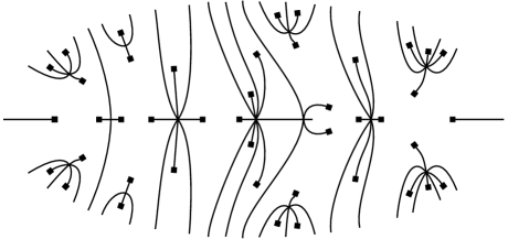
Figure 13: A simple base of type (b) with $\mathfrak{c}=4$, $\mathfrak{o}=3$ and $\mathfrak{e}=2$.

Remark 8.7.

Simple bases are exactly the maximal bases appearing in the proof of Theorem 8.5. Each connected component $Z_{+}$ contained in $\{\Im(z)>0\}$ contains exactly one vertex of degree greater than $2$. Each bounded closed connected component of $B\cap{\mathbf{R}}$ is $\mathfrak{o}$ contains exactly one vertex of degree $4n$ and no two of these vertices carry the same label. They correspond to local maxima and are called the maxima of $B$. There are $\mathfrak{e}$ vertices of degree $4n+2,n>0$, which we call the crossings of $B$. Again, the labels of crossings are pairwise distinct. In type (b), there exists exactly one finite half-closed connected component of $B\cap{\mathbf{R}}$, and it contains no maximum, but at least one crossing. In particular, if $\mathfrak{e}=0$, simple bases of type (b) do not exist. However, simple bases of type (b) do exist if $\mathfrak{e}>0$, as well as simple bases of type (c) for any value of $\mathfrak{e}$ (cf. their polynomial counterparts defined in [IZ18, Section 5]). Examples are given in Figures 13 and 14.

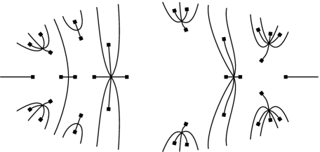
Figure 14: A simple base of type (c) with $\mathfrak{c}=4$, $\mathfrak{o}=3$ and $\mathfrak{e}=0$.

It is now easy to the describe the coefficients in front of the monomials corresponding to the upper bounds in Proposition 8.3. Let $\mathbf{SB}_{(B)}$ and $\mathbf{SB}_{(C)}$ denote the set of simple bases of type (b) and type (c), respectively. We defined signs on these sets in Definition 7.8 and can take the signed counts $S(\mathbf{SB}_{(B)})$ and $S(\mathbf{SB}_{(C)})$.

Corollary 8.8.

The coefficients of the monomials corresponding to $f$-degree $(\mathfrak{c}+1,\mathfrak{c}+\mathfrak{o}+2)$, $g$-degree $(\mathfrak{c},\mathfrak{c}+\mathfrak{o}+2)$, for $d$ odd, and $f$-degree $(\mathfrak{c},\mathfrak{c}+\mathfrak{o}+2)$, $g$-degree $(\mathfrak{c}+1,\mathfrak{c}+\mathfrak{o}+2)$, for $d$ even, are equal, in the same order, to $\frac{(-1)^{\mathfrak{c}}}{2^{\mathfrak{c}}}$ times

$$S(\mathbf{SB}_{(C)}),\quad S(\mathbf{SB}_{(B)})+2S(\mathbf{SB}_{(C)}),\quad-S(\mathbf{SB}_{(B)})-2S(\mathbf{SB}_{(C)}),\quad S(\mathbf{SB}_{(C)}).$$

Proof.

The statement follows by Proposition 8.3, Theorem 8.5, and Remark 8.7. ∎

8.1 The case $\mathfrak{e}=0$

Lemma 8.9.

If $\mathfrak{e}=0$, no simple bases of type (b) exist, and all simple bases of type (c) have the same sign $(-1)^{\mathfrak{o}}$.

Proof.

The non-existence of bases of type (b) is explained in Remark 8.7. Assume $B$ is a simple base of type (c). Since for each label $j$ there exists at most one real vertex with label $j$, and all of them are maxima (i.e., the non-one entries in $\Sigma_{b_{j}}$ are succeeded by an odd number of $1$’s), each maximum contributes $-1$ to $\varepsilon(B)$, and the claim follows. ∎

8.2 The case $\mathfrak{e}>0$

Definition 8.10.

Given a simple bases $B$, a crossings $v$ and a $2$-valent vertex $w$ of the same label, we denote by $\operatorname{Flip}^{v}_{w}(B)$ the base obtained from $B$ by exchanging the two vertices together with adjacent edges of $v$ in ${\mathbf{C}}\setminus{\mathbf{R}}$. If we flip an “increasing” and a “decreasing” vertex, we also reverse the order of these edges. We denote by $[B]$ the equivalence class of simple bases up to changing the position of the crossings via the flip operation.

Proposition 8.11.

If $\mathfrak{e}$ is a positive integer, then

$$S([B])=\begin{cases}0&d\text{ odd, type \ref{case3} ,}\\ (-1)^{\mathfrak{o}+\mathfrak{b}}&d\text{ odd, type \ref{case2}, }\mathfrak{e}\text{ even, or }d\text{ even, type \ref{case3}.}\end{cases}$$

Here, $\mathfrak{b}$ denotes the number of partitions $\lambda_{i}$ with both an odd and even entry appearing an odd number of times, and the even entry is bigger than the odd entry.

Note that we neglect the case $d$ even, type (b), which is not needed here.

Proof.

The connected components of $B\cap{\mathbf{R}}$ of form $(-\infty,y],[x,+\infty),[x,y]$ and $[x,y)$ or $(x,y]$ are called left end, right end, ordinary segment, special segment in the following. For each crossing, there are zero or two possible positions on an ordinary segment and one position on any other segment. Let $v$ be a crossing (labelled by $j$) sitting on the left end (only if $d$ is odd) or on an ordinary segment. Let $w$ be the $2$-valent vertex of the same label on the right end or on the same ordinary segment. Then $\operatorname{Flip}^{v}_{w}(B)$ has opposite sign. This is clear in the second case and easy to verify in the first case, since the sequence $\Sigma_{j}$ we are manipulating is of the form

$$(a,\underbrace{1,\dots,1}_{\text{even number}},1)\quad\text{ or }\quad(a,\underbrace{1,\dots,1,b,1\dots 1}_{\text{odd number}},1),$$

with $1\neq a\neq b\neq 1$. The second case occurs if and only if there is a maximum with same label as $v$. We can easily turn this into an involution on $[B]$, reducing the computation of $S([B])$ to those bases for which all crossings are located on the special segment, if $B$ is of type (b), and all crossings located on the right end, if $B$ is of type (c) and $d$ is even.
It remains to show that the sign of such bases is $(-1)^{\mathfrak{o}+\mathfrak{b}}$. In the first case (type (b), crossings on special segment), we note that a crossing labelled with $j$ is succeeded by an odd or even number of $1$’s in $\Sigma_{j}$, depending on whether the special segment is of the form $(x,y]$ or $[x,y)$. Since $\mathfrak{e}$ is even, the total contribution of the corresponding disorders is always even. It remains to count the disorders involving a maximum. A maximum labelled by $j$ is succeeded by an odd number $l_{j}$ of entries in $\Sigma_{j}$. If no crossing of label $j$ and higher degree than the maximum exists, the number of disorders involving the maximum is $l_{j}$. If a crossing of higher degree than the maximum exists, then the number of disorders involving the maximum is $l_{j}+1$ or $l_{j}-1$, depending on whether the crossing lies before or after the maximum. Hence the critical levels to be counted are exactly those which contain a maximum, but no crossing of higher degree. The number of such levels is $\mathfrak{o}-\mathfrak{b}$. ∎

8.3 Proofs of main theorems

Proof of Theorem 1.2.

The vanishing statements are contained in Propositions 5.1 and 5.2, and it remains to prove non-vanishing under the given conditions. Fix ${\bm{\lambda}}$ and the parity of $d$ such that the conditions in Theorem 1.2 are satisfied. Recall that Theorem 7.1 asserts that the series $F^{odd}_{{\bm{\lambda}}}(q)$ and $F^{even}_{{\bm{\lambda}}}(q)$ are polynomials in $q$, $f$ and $g$. Therefore, by Proposition 8.1, it suffices to prove that in the $g$-reduced representations of $F^{odd}_{{\bm{\lambda}}}(q)$ and $F^{even}_{{\bm{\lambda}}}(q)$ at least one of the coefficients is non-zero.

$d$ odd, $\mathfrak{e}=0$: By Corollary 8.8 it suffices to show $S(\mathbf{SB}_{(C)})\neq 0$. This follows by Lemma 8.9, since all elements in $\mathbf{SB}_{(C)}$ have the same sign.

$d$ odd, $\mathfrak{e}>0$: By Corollary 8.8 it suffices to show $S(\mathbf{SB}_{(B)})+2S(\mathbf{SB}_{(C)})\neq 0$. This follows by Proposition 8.11, since $S(\mathbf{SB}_{(C)})=0$ and $S(\mathbf{SB}_{(B)})=(-1)^{\mathfrak{o}+\mathfrak{b}}E$, where $E$ denotes the number of equivalence classes in $\mathbf{SB}_{(B)}$.

$d$ even: By Corollary 8.8 it suffices to show $S(\mathbf{SB}_{(C)})\neq 0$. This follows by Propositions 8.9 and 8.11, since $S(\mathbf{SB}_{(C)})=(-1)^{\mathfrak{o}+\mathfrak{b}}E$, where $E$ denotes the number of equivalence classes in $\mathbf{SB}_{(C)}$. This completes the proof. ∎

Remark 8.12.

To compute the numbers $S(\mathbf{SB}_{(B)})$ and $S(\mathbf{SB}_{(C)})$ appearing in the previous proof, we note that simple bases belonging to different equivalence classes differ by the position of s, and the ordering of the pairs of complex conjugate critical points and real critical maxima. Moreover, we need to avoid overcounting bases having two critical points with same multiplicity and label in $\{\Im(z)>0\}$. Denote by $N_{j}^{i}$ the number of times an element $i$ appears in $\lambda_{j}$ and set

$$A({\bm{\lambda}})=\prod_{j=1}^{k}\prod_{i}\lfloor N_{j}^{i}/2\rfloor,$$

where the second product runs through all $i$ with $N_{j}^{i}\geq 2$. Then for all $d$ we have

$$\mathbf{SB}_{(C)}=\frac{\displaystyle(\mathfrak{o}+1)\cdot(\mathfrak{o}+\mathfrak{c})!}{A({\bm{\lambda}})},$$

and for $d$ odd and $\mathfrak{e}>0$ we have

$$\mathbf{SB}_{(B)}=\frac{\displaystyle 2\cdot(\mathfrak{o}+\mathfrak{c}+1)!}{A({\bm{\lambda}})}.$$

Proof of Theorem 1.3.

Since we assume that the non-vanishing criteria from Theorem 1.2 are satisfied, we have $F:=F^{odd}_{{\bm{\lambda}}}\neq 0$ or $F:=F^{even}_{{\bm{\lambda}}}\neq 0$, respectively. By the proof of Proposition 8.1 we conclude that $F$ has bounded convergence radius $\pi/2$, with poles $\pm i\pi/2$ on the boundary circle. Note that $F$ is either an even or an odd function, depending on the parity of $\sum_{i,j}\lambda_{j}^{i}$. Following [IZ18, Proof of Theorem 5], let $G$ denote the function obtained by dividing by $q$, if $F$ is odd, and performing the variable change $Q=q^{2}$. Then $G$ has a unique singularity at radius $\pi^{2}/4$ and hence $\ln|b_{k}|\sim-k\ln(\pi^{2}/4)$, where $b_{k}$ denote the coefficients in $G$. Since $b_{k}=S({\bm{\lambda}},m)/m!$ for $m=2k$ or $m=2k+1$, respectively, the claim follows. ∎

Remark 8.13.

Let $H^{\mathbf{C}}({\bm{\lambda}},m)$ denote the Hurwitz number counting complex simple rational functions $\varphi\in{\mathbf{C}}(z)$ with $k$ critical levels of reduced ramification type $\lambda_{1},\dots,\lambda_{k}$ and $m$ additional simple branch points. We would like to show $\ln H^{\mathbf{C}}({\bm{\lambda}},m)\sim m\ln(m)$ for $m\to\infty$, and hence $\ln H^{\mathbf{C}}({\bm{\lambda}},m)\sim\ln|S({\bm{\lambda}},m)|$ under the non-vanishing assumption of Theorem 1.3.

To prove the claim, we first use the perturbation argument from [Rau19, Proof of Theorem 5.10] to show that

$$H^{\mathbf{C}}({\bm{\lambda}},m)\leq H^{\mathbf{C}}(\emptyset,m+\sum_{i,j}\lambda_{j}^{i}).$$

The right hand side can be computed using the classical formula by Hurwitz for genus $0$ single Hurwitz numbers, see [Hur91, page 22], which gives for $m>1$

$$H^{\mathbf{C}}(\emptyset,m)=(m-1)^{m-1}.$$

Therefore the asymptotics of $\ln H^{\mathbf{C}}({\bm{\lambda}},m)$ is bounded from above by

$$\ln H^{\mathbf{C}}(\emptyset,m)\sim m\ln(m).$$

Then the equivalence follows from a suitable lower bound, e.g. the real count,

$$|S({\bm{\lambda}},m)|\leq 2H^{\mathbf{C}}({\bm{\lambda}},m).$$

The factor $2$ is due to the fact that in the real case we consider oriented functions.

Contact

• Boulos El Hilany, Instytut Matematyczny Polskiej Akademii Nauk, ul. Śniadeckich 8, 00-656 Warszawa, Poland; boulos.hilani@gmail.com.

• Johannes Rau, Universität Tübingen, Geschwister-Scholl-Platz, 72074 Tübingen, Germany; johannes.rau@math.uni-tuebingen.de.

References

- [AN06] Andrei Alexeevski and Sergei Natanzon “Noncommutative two-dimensional topological field theories and Hurwitz numbers for real algebraic curves” In Sel. Math., New Ser. 12.3-4 Springer (Birkhäuser), Basel, 2006, pp. 307–377 arXiv:math/0202164
- [And81] Désiré André “Sur les permutations alternées” In Journal de mathématiques pures et appliquées 7, 1881, pp. 167–184
- [Bar92] Serguei A. Barannikov “On the space of real polynomials without multiple critical values.” In Funct. Anal. Appl. 26.2 Springer US, New York, NY, 1992, pp. 10–17
- [GZ15] Penka Georgieva and Aleksey Zinger “Real Orientations, Real Gromov-Witten Theory, and Real Enumerative Geometry” In ArXiv e-prints, 2015 arXiv:1512.07220
- [GMR16] Mathieu Guay-Paquet, Hannah Markwig and Johannes Rau “The Combinatorics of Real Double Hurwitz Numbers with Real Positive Branch Points” In Int. Math. Res. Not. 2016.1 Oxford University Press, Cary, NC, 2016, pp. 258–293 arXiv:1409.8095
- [Hur91] Adolf Hurwitz “Über Riemann’sche Flächen mit gegebenen Verzweigungspunkten” In Math. Ann. 39 Springer, Berlin/Heidelberg, 1891, pp. 1–61
- [IKS04] Ilia Itenberg, Viatcheslav Kharlamov and Eugenii Shustin “Logarithmic equivalence of the Welschinger and the Gromov-Witten invariants” In Russ. Math. Surv. 59.6 IOP Publishing, 2004, pp. 1093–1116 arXiv:math/0407188
- [IZ18] Ilia Itenberg and Dimitri Zvonkine “Hurwitz numbers for real polynomials” In Comment. Math. Helv. 93.3, 2018, pp. 441–474
- [MR15] Hannah Markwig and Johannes Rau “Tropical Real Hurwitz numbers” In Math. Z. 281.1-2, 2015, pp. 501–522 arXiv:1412.4235
- [NSV02] Sergei Natanzon, Boris Shapiro and Alek Vainshtein “Topological classification of generic real rational functions” In J. Knot Theory Ramifications 11.7 World Scientific, Singapore, 2002, pp. 1063–1075 arXiv:math/0110235
- [Orl17] Aleksander Yu. Orlov “Matrix integrals and Hurwitz numbers” In ArXiv e-prints, 2017 arXiv:1701.02296
- [Rau19] Johannes Rau “Lower bounds and asymptotics of real double Hurwitz numbers” In Math. Ann. 375.1-2, 2019, pp. 895–915
- [Sta10] Richard P. Stanley “A survey of alternating permutations” In Combinatorics and graphs. Selected papers based on the presentations at the 20th anniversary conference of IPM on combinatorics, Tehran, Iran, May 15–21, 2009. Providence, RI: American Mathematical Society (AMS), 2010, pp. 165–196 arXiv:0912.4240
- [Wel05] Jean-Yves Welschinger “Invariants of real symplectic 4-manifolds and lower bounds in real enumerative geometry” In Invent. Math. 162.1 Springer-Verlag, Berlin, 2005, pp. 195–234 arXiv:math/0303145