The two periodic Aztec diamond and matrix valued orthogonal polynomials

Abstract

We analyze domino tilings of the two-periodic Aztec diamond by means of matrix valued orthogonal polynomials that we obtain from a reformulation of the Aztec diamond as a non-intersecting path model with periodic transition matrices. In a more general framework we express the correlation kernel for the underlying determinantal point process as a double contour integral that contains the reproducing kernel of matrix valued orthogonal polynomials. We use the Riemann-Hilbert problem to simplify this formula for the case of the two-periodic Aztec diamond.

In the large size limit we recover the three phases of the model known as solid, liquid and gas. We describe fine asymptotics for the gas phase and at the cusp points of the liquid-gas boundary, thereby complementing and extending results of Chhita and Johansson.

1 Introduction

We study domino tilings of the Aztec diamond with a two periodic weighting. This model falls into a class of models for which existing techniques for studying fine asymptotics are not adequate and only recently first important progress has been made [9, 20]. We introduce a new approach based on matrix valued orthogonal polynomials that allows us to compute the determinantal correlations at finite size and their asymptotics as the size of the diamond gets large in a rather orderly way. We strongly believe that this approach will also prove to be a good starting point for other tiling models with a periodic weighting.

Random tilings of planar domains have been studied intensively in the past decade. Such models exhibit a rich structure including a limit shape and fluctuations that are expected to fall in various important universality classes (see [8, 22, 23, 43, 45, 46, 47, 48] for general references on the topic and [18, 58, 59] for recent contributions). When the correlation structure is determinantal, there is hope to understand the fine asymptotic structure by studying the asymptotic behavior of the correlation kernel. An important source of examples of such models is the Schur process [56]. For these models the correlation kernel can be explicitly computed in terms of a double integral representation, opening up to the possibility of performing an asymptotic analysis by means of classical steepest decent (or stationary phase) techniques.

Of course, the Schur process is rather special and many models of interest fall outside this class. In particular this is true for random tilings or dimer models with doubly periodic weightings. Yet, these models have exciting new features and have therefore been discussed in the physics and mathematics literature [9, 20, 21, 36, 48, 55]. An important feature is the appearance of a so-called gas phase. For instance, in the two periodic weighting for domino tiling of the Aztec diamond, the diamond can be partitioned into three regions: the solid, liquid and gas region [56] (as we will see in Figure 7 below). The gas region has not been observed in models that are in the Schur class. The $2$-point correlations (for an associated particle process) in the gas region behave differently when compared to the liquid regions. Indeed, the correlation kernel decays exponentially with the distance $d$ between the points, instead of $\sim 1/d$ in the liquid region. At the liquid-solid boundary one expects the Airy process to appear, but the situation at the gas-liquid boundary is far more complicated [9, 20].

To the best of our knowledge, the two periodic Aztec diamond is the only model with periodic weightings for which rigorous results on fine asymptotics exist [9, 20]. Inspired by a formula for the Kasteleyn matrix found by Chhita and Young [21], Chhita and Johansson [20] found a way to compute the asymptotic behavior of the Kasteleyn matrix as the size of the Aztec diamond goes to infinity. We will follow a different approach to studying such models with periodic weightings.

As we will recall in Section 3, the Aztec diamond can be described by non-intersecting paths (we refer to [45] and the references therein for more background on the relation between dimers, tilings, non-intersecting paths and all that). For a general class of discrete non-intersecting paths with $p$-periodic transition matrices (which includes $p$-periodic weightings for domino tilings of the Aztec diamond and $p$-periodic weightings for lozenge tilings of the hexagon), we show in Section 4 how the correlation kernel can be written as a double integral formula involving matrix valued polynomials that satisfy a non-hermitian orthogonality.

We believe that this general setup has a high potential for a rigorous asymptotic analysis. The key fact is that these matrix valued orthogonal polynomials can be characterized in terms of the solution of a $2p\times 2p$ matrix valued Riemann-Hilbert problem. With the highly developed Riemann-Hilbert toolkit at hand, we may thus hope to compute the asymptotic behavior of the polynomials, and more importantly the correlation kernel. The formalism will be worked out in Section 4. It provides a new perspective even on the classical examples of uniform domino tilings of the Aztec diamond and lozenge tilings of a hexagon, as we will discuss briefly in Sections 4.7 and 4.8.

The main focus of the paper is to show how the Riemann-Hilbert approach can be exploited to find an asymptotic analysis for the two periodic Aztec diamond. Remarkably, in this case the result of the Riemann-Hilbert analysis is a surprisingly simple double integral formula for the correlation kernel. It is not an asymptotic result, but an exact formula valid for fixed finite $N$. This representation also appears to be more elementary than the one given in Chhita and Johansson [20]. The Riemann-Hilbert analysis is given in Section 5. We analyze the double integral formula for the kernel asymptotically using classical steepest descent techniques in Section 6.

The model of the two periodic Aztec diamond is explained and the main results are summarized in the next section.

2 Statement of results

In this section we will introduce the two periodic Aztec diamond and state our main results for this model.

2.1 Definition of the model

The Aztec diamond is a region on the square lattice with a sawtooth boundary that can be covered by $2\times 1$ and $1\times 2$ rectangles, called dominos. The squares have a black/white checkerboard coloring and a possible tiling of the Aztec diamond of size $4$ is shown in Figure 1. There are four types of dominos, namely North, West, East, and South, that are also shown in the figure. The Aztec diamond model was first introduced in [33].

Figure 1: Possible tiling of a $4\times 4$ Aztec diamond with four kinds of dominos.

In the two periodic Aztec diamond we assign a weight to each domino in a tiling, depending on its shape (horizontal or vertical) and its location in the Aztec diamond. We assume the Aztec diamond is of even size.

To describe the two periodic weighting we introduce a coordinate system where $(0,0)$ is at the center of the Aztec diamond. The center of a horizontal domino has coordinates $(x,y+1/2)$ with $x,y\in\mathbb{Z}$. We then say that the horizontal domino is in column $x$. The center of a vertical domino has coordinates $(x+1/2,y)$ with $x,y\in\mathbb{Z}$, and we say that the vertical domino is in row $y$. The row and column numbers run from $-N+1$ to $N-1$, where $2N$ is the size of the Aztec diamond.

We fix two positive numbers $a$ and $b$ and define the weights as follows.

Definition 2.1.

The weight of a domino $D$ in a tiling $\mathcal{T}$ of the Aztec diamond is

$$w(D)=\begin{cases}a,&\text{if $D$ is a horizontal domino in an even column},\\ b,&\text{if $D$ is a horizontal domino in an odd column},\\ b,&\text{if $D$ is a vertical domino in an even row},\\ a,&\text{if $D$ is a vertical domino in an odd row}.\end{cases}$$ (2.1)

The weight of the tiling $\mathcal{T}$ is

$$w(\mathcal{T})=\prod_{D\in\mathcal{T}}w(D),$$ (2.2)

and the probability for $\mathcal{T}$ is

$$\mathcal{P}(\mathcal{T})=\frac{w(\mathcal{T})}{Z_{N}},$$ (2.3)

where $Z_{N}=\sum\limits_{\mathcal{T}^{\prime}}w(\mathcal{T}^{\prime})$ (sum over all possible tilings $\mathcal{T}^{\prime}$ of an Aztec diamond of size $2N$) is the partition function.

In the example from Figure 1 the weights are shown in Figure 2. The weight of the tiling is $w(\mathcal{T})=a^{10}b^{10}$.

Figure 2: Two periodic weights of dominos in a tiling of the Aztec diamond. The vertical dominos in an even row and the horizontal dominos in an odd column have weight $a$. Other dominos have weight $b$.

The model is homogeneous in the sense that the probabilities (2.3) do not change if we multiply $a$ and $b$ by a common factor. We may and do assume $ab=1$. In what follows it will be more convenient to work with

$$\alpha=a^{2},\qquad\beta=b^{2}$$ (2.4)

instead of $a$ and $b$. We have $\alpha\beta=1$, and without loss of generality we assume $\alpha\geq 1$. If $\alpha=\beta=1$ then the model reduces to the uniform weighting on domino tilings, and so the true interest is in the case $\alpha>1$, and this is what we assume from now on.

2.2 Particle system and determinantal point process

By putting a particle in the black square of the West and South dominos, we obtain a random particle system. In our running example the particle systems is shown in Figure 3.

Figure 3: Particles in a domino tiling.

We rotate the picture over 45 degrees in clockwise direction and we change the coordinate system so that black squares are identified with the product set

$$\mathcal{B}_{N}=\{0,\ldots,2N\}\times\{0,\ldots,2N-1\}$$ (2.5)

Any possible tiling of the Aztec diamond gives rise to a subset $\mathcal{X}=\mathcal{X}(\mathcal{T})$ of $\mathcal{B}_{N}$ containing the squares that are occupied by a particle.

We use $(m,n)\in\mathcal{B}_{N}$ to denote an element $\mathcal{B}_{N}$ and we will refer to $m$ as the level in $\mathcal{B}_{N}$. Any $\mathcal{X}$ that comes from a tiling will have $2N-m$ particles at level $m$ for each $m=0,1,\ldots,2N$. Therefore the cardinality is

$$|\mathcal{X}|=N(2N+1).$$

There are also interlacing conditions that are satisfied when comparing the particles at level $m$ with those at level $m+1$.

The probability measure (2.3) on tilings gives rise to a probability measure on subsets $\mathcal{X}$, that turns out to be determinantal. This means that there exists a kernel

$$K_{N}:\mathcal{B}_{N}\times\mathcal{B}_{N}\to\mathbb{R}$$ (2.6)

with the property that for any subset $S\subset\mathcal{B}_{N}$

$$\mathcal{P}\left[S\subset\mathcal{X}\right]=\det\left[K_{N}(x,y)\right]_{x,y\in S}.$$

This is a discrete determinantal point process [15].

We found an explicit double contour integral formula for the kernel $K_{N}$. We take $(m,n),(m^{\prime},n^{\prime})\in\mathcal{B}_{N}$, and instead of $K_{N}((m,n),(m^{\prime},n^{\prime}))$ we write $K_{N}(m,n;m^{\prime},n^{\prime})$. We collect $K_{N}(m,n;m^{\prime},n^{\prime})$ with some of its neighbors in a $2\times 2$ matrix

$$\mathbb{K}_{N}(m,n;m^{\prime},n^{\prime})=\begin{pmatrix}K_{N}(m,n;m^{\prime},n^{\prime})&K_{N}(m,n+1;m^{\prime},n^{\prime})\\ K_{N}(m,n;m^{\prime},n^{\prime}+1)&K_{N}(m,n+1;m^{\prime},n^{\prime}+1)\end{pmatrix}$$ (2.7)

and this matrix appears in our formula (2.8).

Theorem 2.2.

Assume $N$ is even and $(m,n)\in\mathcal{B}_{N}$, $(m^{\prime},n^{\prime})\in\mathcal{B}_{N}$ are such that $m+n$ and $m^{\prime}+n^{\prime}$ are even. Then

$$\mathbb{K}_{N}(m,n;m^{\prime},n^{\prime})=-\frac{\chi_{m>m^{\prime}}}{2\pi i}\oint_{\gamma_{0,1}}A^{m-m^{\prime}}(z)z^{(m^{\prime}+n^{\prime})/2-(m+n)/2}\frac{dz}{z}\\ +\frac{1}{(2\pi i)^{2}}\oint_{\gamma_{0,1}}\frac{dz}{z}\oint_{\gamma_{1}}\frac{dw}{z-w}A^{N-m^{\prime}}(w)F(w)A^{-N+m}(z)\\ \times\frac{z^{N/2}(z-1)^{N}}{w^{N/2}(w-1)^{N}}\frac{w^{(m^{\prime}+n^{\prime})/2}}{z^{(m+n)/2}}$$ (2.8)

where

$$A(z)=\frac{1}{z-1}\begin{pmatrix}2\alpha z&\alpha(z+1)\\ \beta z(z+1)&2\beta z\end{pmatrix}$$ (2.9)

and

$$F(z)=\frac{1}{2}I_{2}+\frac{1}{2\sqrt{z(z+\alpha^{2})(z+\beta^{2})}}\begin{pmatrix}(\alpha-\beta)z&\alpha(z+1)\\ \beta z(z+1)&-(\alpha-\beta)z\end{pmatrix},$$ (2.10)

where $I_{2}$ denotes the $2\times 2$ identity matrix and we use the principal branch of the square root in (2.10). The notation $\chi$ in (2.8) denotes the indicator function, $\chi_{m>m^{\prime}}=1$ if $m>m^{\prime}$ and $\chi_{m>m^{\prime}}=0$ otherwise.

The contour $\gamma_{0,1}$ in (2.8) is a simple closed contour going around $0$ and $1$ in positive direction. The contour $\gamma_{1}$ is a simple closed contour in the right half-plane that goes around $1$ in positive direction, and it lies in the interior of $\gamma_{0,1}$, see Figure 4.

Figure 4: Contours $\gamma_{0,1}$ and $\gamma_{1}$ used in the definition of $\mathbb{K}_{N}$ in (2.8) in Theorem 2.2.

Remark 2.3.

The square root factor in (2.10) is defined and analytic for $z\in\mathbb{C}\setminus((-\infty,-\alpha^{2}]\cup[-\beta^{2},0])$ with the branch that is positive for real $z>0$. This is one sheet of the Riemann surface $\mathcal{R}$ associated with the cubic equation

$$y^{2}=z(z+\alpha^{2})(z+\beta^{2}),$$ (2.11)

that will play an important role in what follows. It is a two sheeted surface consisting of two sheets $\mathbb{C}\setminus((-\infty,-\alpha^{2}]\cup[-\beta^{2},0])$ glued together along the two cuts $(-\infty,-\alpha^{2}]$ and $[-\beta^{2},0]$ in the usual crosswise manner. The surface has genus $1$ unless $\alpha=\beta=1$ in which case the genus drops to $0$.

The matrix valued function $F(z)$ from (2.10) is considered on the first sheet. Its analytic continuation to the second sheet is given by $I_{2}-F(z)$.

Remark 2.4.

The eigenvalues of $A(z)$, see (2.9), are equal to $\frac{\rho_{1,2}(z)}{z-1}$ where

$$\rho_{1,2}(z)=(\alpha+\beta)z\pm\sqrt{z(z+\alpha^{2})(z+\beta^{2})}.$$ (2.12)

are the eigenvalues of $\begin{pmatrix}2\alpha z&\alpha(z+1)\\ \beta z(z+1)&2\beta z\end{pmatrix}$. Thus (2.12) are the two branches of the meromorphic function $\rho=(\alpha+\beta)z+y$ on the Riemann surface $\mathcal{R}$ associated with (2.11), with $\rho_{1}$ on the first sheet and $\rho_{2}$ on the second sheet.

The eigenvectors can also be considered on the Riemann surface. There is a matrix $E(z)$ whose columns are the eigenvectors such that

$$A(z)=\frac{1}{z-1}E(z)\begin{pmatrix}\rho_{1}(z)&0\\ 0&\rho_{2}(z)\end{pmatrix}E^{-1}(z).$$ (2.13)

See (5.6) below for the precise formula for $E(z)$. It turns out that (see (2.10) for the definition of $F(z)$)

$$F(z)=E(z)\begin{pmatrix}1&0\\ 0&0\end{pmatrix}E^{-1}(z).$$ (2.14)

Thus $F(z)$ has eigenvalues $0$ and $1$, and $F(z)$ commutes with $A(z)$.

We will also work with

$$W(z)=\frac{A^{2}(z)}{z}$$ (2.15)

which in view of (2.13) has eigenvalue decomposition

$$W(z)=E(z)\Lambda(z)E^{-1}(z),\qquad\Lambda(z)=\begin{pmatrix}\lambda_{1}(z)&0\\ 0&\lambda_{2}(z)\end{pmatrix}$$ (2.16)

with

$$\lambda_{1,2}(z)=\frac{\rho_{1,2}^{2}(z)}{z(z-1)^{2}}.$$ (2.17)

These eigenvalues are the two branches of a meromorphic function $\lambda$ on the Riemann surface $\mathcal{R}$, with $\lambda_{1}$ defined on the first sheet and $\lambda_{2}$ on the second sheet.

Remark 2.5.

The only singularity for the $w$ integral in (2.8) that is inside the contour $\gamma_{1}$ is the pole at $w=1$. Because of (2.9) we see that $A^{N-m^{\prime}}(w)$ has a pole of order $N-m^{\prime}$ (it is a zero if $m^{\prime}>N$) and therefore the integrand in the double integral of (2.8) has a pole of order $N-m^{\prime}+N=2N-m^{\prime}$ at $w=1$. There is no pole if $m^{\prime}=2N$, and thus it follows that (2.8) vanishes identically for $m^{\prime}=2N$. This is in agreement with the fact that there are no particles at level $2N$.

Level $0$ is full of particles, which means that $K_{N}(0,n;0,n)=1$ for all $n=0,\ldots,2N-1$. This can be seen from formula (2.8) as follows. For $n$ even, the formula gives for $\mathbb{K}_{N}(0,n;0,n)$,

$$\frac{1}{(2\pi i)^{2}}\oint_{\gamma_{0,1}}\frac{dz}{z}\oint_{\gamma_{1}}\frac{dw}{z-w}A^{N}(w)F(w)A^{-N}(z)\frac{z^{N/2}(z-1)^{N}}{w^{N/2}(w-1)^{N}}\frac{w^{n/2}}{z^{n/2}}$$ (2.18)

In view of (2.14), (2.15), and (2.16) we have

$$A^{N}(w)F(w) =w^{N/2}F(w)\lambda_{1}^{N/2}(w),$$ (2.19)

$$A^{N}(w)(I_{2}-F(w)) =w^{N/2}(I_{2}-F(w))\lambda_{2}^{N/2}(w).$$ (2.20)

We will see in Lemma 5.2 (b) that $\lambda_{1}(w)$ has a double pole and $\lambda_{2}(w)$ has a double zero at $w=1$. There are no other zeros and poles. Thus (2.19) has a pole of order $N$ at $w=1$, and (2.20) has a zero of order $N$ at $w=1$. It follows that the $w$-integrand in (2.18) has a pole of order $2N$ at $w=1$. However, if we replace $F(w)$ by $I_{2}-F(w)$, then the integrand does not have a pole at $w=1$ anymore, and thus by Cauchy’s theorem the double integral is zero.

It follows that the value of the double integral (2.18) remains the same if we remove the factor $F(w)$. Then the integrand that remains is rational in $w$, with a simple pole at $w=z$ and a decay $O(w^{-1-N+n/2})$ as $w\to\infty$. We apply the residue theorem to the exterior of $\gamma_{1}$ and the only contribution comes from the pole at $w=z$. The $z$-integral that remains in (2.18) reduces to

$$\frac{1}{2\pi i}\oint_{\gamma_{0,1}}\frac{dz}{z}I_{2}=I_{2}$$

and so by looking at the diagonal entries, see (2.7), we get $K_{N}(0,n;0,n)=K_{N}(0,n+1;0,n+1)=1$, as claimed.

Figure 5: Extended particle system that is equivalent to a domino tiling of the Aztec diamond.

Remark 2.6.

Observe that the particle system on the black squares is not equivalent to the tiling of the Aztec diamond. However, it can be extended to a larger system where we also also put a particle in the white square of the West and South dominos, as shown in Figure 5. This extended process is equivalent to the tiling. It is also determinantal and we will now give a double contour integral formula for the kernel. We chose to work with the particle system determined by the black squares only since the formulas and their asymptotics stated in the next paragraphs take an easier form. The analogous asymptotics for the extended processes are straightforward from these results and the formula (2.25) below.

So in addition to the set of black squares (2.5) we also consider the white squares

$$\mathcal{W}_{N}=\{\tfrac{1}{2},\ldots,2N-\tfrac{1}{2}\}\times\{-\tfrac{1}{2},\tfrac{1}{2},\ldots,2N-\tfrac{1}{2}\}.$$ (2.21)

Then the extended particle system has a correlation kernel (that we continue to denote by $K_{N}$)

$$K_{N}:\left(\mathcal{B}_{N}\cup\mathcal{W}_{N}\right)\times\left(\mathcal{B}_{N}\cup\mathcal{W}_{N}\right)\to\mathbb{R}.$$ (2.22)

To write down the extended kernel we use the notation that will also be used later in (3.3) and (3.5), namely, for an integer $m\in\mathbb{Z}$,

$$A_{m,m+1/2}(z)=\begin{pmatrix}\alpha&\alpha\\ \beta z&\beta\end{pmatrix},\quad A_{m+1/2,m+1}(z)=\frac{1}{z-1}\begin{pmatrix}z&1\\ z&z\end{pmatrix},$$ (2.23)

and for $m,m^{\prime}\in\frac{1}{2}\mathbb{Z}$,

$$A_{m,m^{\prime}}(z)=A_{m,m+1/2}(z)A_{m+1/2,m+1}(z)\cdots A_{m^{\prime}-1/2,m^{\prime}}(z),\quad\text{ if }m<m^{\prime},$$ (2.24)

$A_{m,m^{\prime}}(z)=A_{m^{\prime},m}(z)^{-1}$ if $m>m^{\prime}$, and $A_{m,m}(z)=I_{2}$.

Then the extended kernel (2.22) is as follows. We assume $N$ is even $(m,n)\in\mathcal{B}_{N}\cup\mathcal{W}_{N}$ and $(m^{\prime},n^{\prime})\in\mathcal{B}_{N}\cup\mathcal{W}_{N}$ with both $m+n$ and $m^{\prime}+n^{\prime}$ even. Then

$$\begin{pmatrix}K_{N}(m,n;m^{\prime},n^{\prime})&K_{N}(m,n+1;m^{\prime},n^{\prime})\\ K_{N}(m,n;m^{\prime},n^{\prime}+1)&K_{N}(m,n+1;m^{\prime},n^{\prime}+1)\end{pmatrix}\\ =-\frac{\chi_{m>m^{\prime}}}{2\pi i}\oint_{\gamma_{0,1}}A_{m^{\prime},m}(z)z^{(m^{\prime}+n^{\prime})/2-(m+n)/2}\frac{dz}{z}\\ +\frac{1}{(2\pi i)^{2}}\oint_{\gamma_{0,1}}\frac{dz}{z}\oint_{\gamma_{1}}\frac{dw}{z-w}A_{m^{\prime},N}(w)F(w)A_{N,m}(z)\\ \times\frac{z^{N/2}(z-1)^{N}}{w^{N/2}(w-1)^{N}}\frac{w^{(m^{\prime}+n^{\prime})/2}}{z^{(m+n)/2}}.$$ (2.25)

Observe that by (2.9) and (2.22)

$$A_{m,m+1/2}(z)A_{m+1/2,m+1}(z)=A(z),\qquad m\in\mathbb{Z},$$

and so by the definition (2.24), we have $A_{m^{\prime},m}(z)=A^{m-m^{\prime}}(z)$, $A_{m^{\prime},N}(w)=A^{N-m^{\prime}}(w)$, $A_{N,m}(z)=A^{-N+m}(z)$, if $m,m^{\prime}$ are integers. In this way we recover (2.8) from (2.25).

2.3 Matrix valued orthogonal polynomials

The starting point of our approach to Theorem 2.2 is the non-intersecting path reformulation of the Aztec diamond and the Lindström-Gessel-Viennot lemma. This will be developed in Section 3. The novel ingredient in the further analysis is the use of matrix valued orthogonal polynomials (MVOP).

A matrix valued polynomial of degree $k$ and size $d$ is a function

$$P(z)=C_{0}z^{k}+C_{1}z^{k-1}+\cdots+C_{k}$$

where $C_{0},\ldots,C_{k}$ are matrices of size $d\times d$. Suppose $w(z)$ is a $d\times d$ weight matrix on a set $\Gamma$ in the complex plane.

Definition 2.7.

Suppose $P_{N}$ is a matrix valued polynomial of degree $N$ with an invertible leading coefficient. Then $P_{N}$ is a matrix valued orthogonal polynomial with weight matrix $w$ on $\Gamma$ if

$$\int_{\Gamma}P_{N}(z)w(z)Q^{t}(z)dz=0_{d},$$ (2.26)

for all matrix polynomials $Q$ of degree $\leq N-1$, where $Q^{t}$ denotes the matrix transpose.

The integral in (2.26) is to be taken entrywise, and $0_{d}$ denotes the $d\times d$ zero matrix. We note that the order of the factors in the integrand in (2.26) is important since we are dealing with matrices.

For us the weight matrix will be $\frac{1}{2\pi i}W^{N}(z)$ on the closed contour $\gamma_{1}$ around $1$. Thus $d=2$, and $W^{N}$ denotes the $N$th power of $W$, so that the weight matrix is varying with $N$. Recall that $W$ is defined in (2.15), and explicitly we have

$$W(z)=\frac{1}{(z-1)^{2}}\begin{pmatrix}(z+1)^{2}+4\alpha^{2}z&2\alpha(\alpha+\beta)(z+1)\\ 2\beta(\alpha+\beta)z(z+1)&(z+1)^{2}+4\beta^{2}z\end{pmatrix}.$$ (2.27)

The existing literature on MVOP mostly deals with the case of orthogonality on an interval of the real line, with a positive definite weight matrix $w$ with all existing moments. In such a case the MVOP exists for every degree $n$, and they can be normalized in such a way that

$$\int_{\Gamma}P_{n}(z)w(z)P_{n}^{t}(z)dz=I_{d},\qquad j=0,1,\ldots,n-1.$$ (2.28)

However, it is interesting to note that MVOP first appeared in connection with prediction theory where the orthogonality is on the unit circle, see [11] for a recent survey. The interest in MVOP on the real line has been steadily growing since the early 1990s. The analytic theory of MVOP on the real line is surveyed in [25] with [6] as one of the pioneering works. MVOP satisfy recurrence relations [32] and special cases satisfy differential equations [31]. Interesting examples of MVOP come from matrix valued spherical functions, see [39, 49] as well as many other papers.

We deviate from the usual set-up of MVOP in several ways

• $\Gamma$ is a closed contour in the complex plane,

• the weight matrix $w(z)=\frac{1}{2\pi i}W^{N}(z)$ is complex-valued on $\Gamma$ and varies with $N$,

• the weight matrix is not symmetric or Hermitian (let alone positive definite), or have any other property that would imply existence and uniqueness of the MVOP.

Since there is no complex conjugation in (2.26), we are thus dealing with non-Hermitian matrix valued orthogonality with varying weights on a closed contour in the plane.

As already noted, existence and uniqueness of the MVOP are not guaranteed in this general setting. However, for the weight $\frac{1}{2\pi i}W^{N}$ we can show that the monic MVOP up to degrees $N$ all exist and are unique. However, since the weight matrix is not symmetric, we cannot normalize to obtain orthonormal MVOP as in (2.28). In our case the MVOP of degrees $>N$ do not exist.

In Section 4 we consider a situation that is more general than the two periodic Aztec diamond. It deals with a multi-level particle system that is determinantal, and transitions between the levels are periodic. See Assumptions 4.1 and 4.2 for the precise assumptions. In this general setting we make a connection with matrix valued (bi)orthogonal polynomials and our main result in Section 4 is Theorem 4.7 that expresses the correlation kernel as a double contour integral containing a reproducing kernel for the matrix polynomials.

In the special situation of the two periodic Aztec diamond it gives that the matrix $\mathbb{K}_{N}$ with the correlation kernels as in (2.8) is given by

$$-\frac{\chi_{m>m^{\prime}}}{2\pi i}\oint_{\gamma_{0,1}}A^{m-m^{\prime}}(z)z^{(m^{\prime}+n^{\prime})/2-(m+n)/2}\frac{dz}{z}\\ +\frac{1}{(2\pi i)^{2}}\oint_{\gamma_{0,1}}\frac{dz}{z}\oint_{\gamma_{0,1}}\frac{dw}{z-w}A^{2N-m^{\prime}}(w)R_{N}(w,z)A^{m}(z)\frac{w^{(m^{\prime}+n^{\prime})/2}}{z^{(m+n)/2}w^{N}}.$$ (2.29)

where $R_{N}(w,z)$ is the reproducing kernel associated with the matrix polynomials of degrees $\leq N-1$. That is, $R_{N}(w,z)$ is a bivariate matrix valued polynomial of degree $N-1$ in both $w$ and $z$, such that

$$\frac{1}{2\pi i}\oint_{\gamma_{1}}R_{N}(w,z)W^{N}(z)Q^{t}(z)dz=Q^{t}(w)$$

holds for every matrix valued polynomial $Q$ of degree $\leq N-1$.

The MVOP of degree $N$ is characterized by a Riemann-Hilbert problem and the reproducing kernel $R_{N}(w,z)$ can be expressed in terms of the solution of the Riemann-Hilbert problem. This is known from work of Delvaux [29] and we recall it in Section 4.6. Then we perform an analysis of the Riemann-Hilbert problem, and quite remarkably this produces the exact formula (2.8).

2.4 Classification of phases

The explicit formula (2.8) in Theorem 2.2 is suitable for asymptotic analysis as $N\to\infty$. See Figure 6 for a sampling of a large 2-periodic Aztec diamond. In this figure three regions emerge where the tiling appears to have different statistical behavior. We first describe how we can distinguish these three phases (solid, liquid and gas) in the model. This classification will depend on the location of saddle points for the double integral in (2.8).

Figure 6: A sample of a two-periodic Aztec diamond of size $500$. We colored the West and South dominos blue. The East and North dominons are colored yellow. The gas phase is visible in the middle. This figure is generated by a code that was kindly provided to us by Sunil Chhita.

We fix coordinates $-1<\xi_{1}<1$ and $-1<\xi_{2}<1$ and choose $m,m^{\prime}\approx(1+\xi_{1})N$ and $n,n^{\prime}\approx(1+\xi_{2})N$. Then from the formula (2.8), we see that the $z$ integral of the double contour integral is dominated as $N\to\infty$ by the expression

$$A(z)^{\xi_{1}N}z^{N/2}(z-1)^{N}z^{-(1+\frac{\xi_{1}}{2}+\frac{\xi_{2}}{2})N}=W^{\xi_{1}N/2}(z)(z-1)^{N}z^{-(1+\xi_{2})N/2}$$

where $W$ is given by (2.15). In view of the eigenvalue decomposition (2.16) this is

$$E(z)\begin{pmatrix}e^{N\Phi_{1}(z)/2}&0\\ 0&e^{N\Phi_{2}(z)/2}\end{pmatrix}E(z)^{-1}$$

with $\Phi_{j}(z)=2\log(z-1)-(1+\xi_{2})\log z+\xi_{1}\log\lambda_{j}(z)$, $j=1,2$. Hence we are led to consider

$$\Phi(z)=2\log(z-1)-(1+\xi_{2})\log z+\xi_{1}\log\lambda(z)$$ (2.30)

as a function on the Riemann surface $\mathcal{R}$, depending on parameters $\xi_{1}$ and $\xi_{2}$. It is multi-valued, but its differential

$$\Phi^{\prime}(z)dz=\left(\frac{2}{z-1}-\frac{1+\xi_{2}}{z}+\xi_{1}\frac{\lambda^{\prime}(z)}{\lambda(z)}\right)dz$$ (2.31)

is a single-valued meromorphic differential with simple poles at $z=1^{(1)}$, $z=1^{(2)}$, $z=0$ and $z=\infty$, see also Section 6.2. (For $j=1,2$, we use $1^{(j)}$ to denote the value $1$ on the $j$th sheet of the Riemann surface.) There are also four zeros, counting multiplicities, since the genus is $1$.

Definition 2.8.

The saddle points are the zeros of $\Phi^{\prime}(z)dz$.

The real part $\mathcal{R}_{r}$ of the Riemann surface consists of all real tuples $(z,y)$ satisfying the algebraic equation (2.11) together with the point at infinity. The real part is the union of two cycles,

$$\mathcal{R}_{r}=\mathcal{C}_{1}\cup\mathcal{C}_{2}$$ (2.32)

where $\mathcal{C}_{1}$ is the union of the intervals $[-\alpha^{2},-\beta^{2}]$ on the two sheets, and $\mathcal{C}_{2}$ is the union of the two intervals $[0,\infty]$ on both sheets.

It turns out that there are always at least two distinct saddle points on the cycle $\mathcal{C}_{1}$, see Proposition 6.4 below. The location of the other two saddle points determines the phase.

Definition 2.9.

Let $-1<\xi_{1},\xi_{2}<1$.

• If two simple saddles are in $\mathcal{C}_{2}$, then $(\xi_{1},\xi_{2})$ is in the solid phase, and we write $(\xi_{1},\xi_{2})\in\mathfrak{S}$.

• If two saddles are outside of the real part of the Riemann surface, then $(\xi_{1},\xi_{2})$ is in the liquid phase, and we write $(\xi_{1},\xi_{2})\in\mathfrak{L}$ .

• If all four saddles are simple and belong to $\mathcal{C}_{1}$, then $(\xi_{1},\xi_{2})$ is in the gas phase, and we write $(\xi_{1},\xi_{2})\in\mathfrak{G}$.

Transitions between phases take place when two or more saddle points coalesce.

• If there is a double saddle point on $\mathcal{C}_{2}$, then $(\xi_{1},\xi_{2})$ is on the solid-liquid transition.

• If there is a double or triple saddle point on $\mathcal{C}_{1}$ then $(\xi_{1},\xi_{2})$ is on the liquid-gas transition.

It is not possible to have a double saddle point outside of the real part of the Riemann surface.

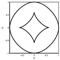
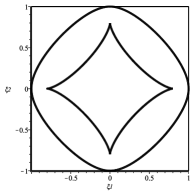
Figure 7: Real section of the degree 8 algebraic curve in $\xi_{1}$-$\xi_{2}$ plane for the cases $\alpha=2$ (left) and $\alpha=3$ (right). The outer component is the boundary between the solid and liquid phases and the inner component is the boundary between the liquid and gas phases.

The condition for coalescing saddle points leads to an algebraic equation of degree $8$ for $\xi_{1},\xi_{2}$ and it precisely coincides with the equation listed in the appendix of [20], see also (6.10) below.

The real section of the degree 8 algebraic equation has two components in case $\alpha>1$, as shown in Figure 7. Both components are contained in the square $-1\leq\xi_{1},\xi_{2}\leq 1$. The outer component is a smooth closed curve that touches the square in the points $(\pm 1,0)$, and $(0,\pm 1)$. It is the boundary between the solid and liquid phases.

The inner component is the boundary between the liquid and gas phases. It is a closed curve with four cusps at locations $\left(\pm\tfrac{\alpha-\beta}{\alpha+\beta},0\right)$, and $\left(0,\pm\tfrac{\alpha-\beta}{\alpha+\beta}\right)$.

It can indeed be checked that for $\xi_{1}=0$, the eight solutions of the degree $8$ equation for $\xi_{2}$ are explicit, namely $\xi_{2}=\pm 1$ with multiplicity $1$ and $\xi_{2}=\pm\frac{\alpha-\beta}{\alpha+\beta}$, both with multiplicity $3$.

The intersections of the algebraic curve with the diagonal lines $\xi_{2}=\pm\xi_{1}$ are explicit as well, namely $(\xi_{1},\xi_{2})=\left(\pm\tfrac{\alpha+1}{2\sqrt{\alpha^{2}+1}},\pm\tfrac{\alpha+1}{2\sqrt{\alpha^{2}+1}}\right)$ are on the outer component, and $(\xi_{1},\xi_{2})=\left(\pm\tfrac{\alpha-1}{2\sqrt{\alpha^{2}+1}},\pm\tfrac{\alpha-1}{2\sqrt{\alpha^{2}+1}}\right)$ are on the inner component.

2.5 Gas phase

Our next result gives the limit of $\mathbb{K}_{N}$ in the gas phase. Recall that $\mathbb{K}_{N}$ is defined by (2.7).

Theorem 2.10.

Assume $(\xi_{1},\xi_{2})\in\mathfrak{G}$. Suppose $m,m^{\prime},n,n^{\prime}$ are integers that vary with $N$ in such a way that

$$m=(1+\xi_{1})N+o(N),\quad n=(1+\xi_{2})N+o(N),$$ (2.33)

as $N\to\infty$, while

$$m^{\prime}-m=\Delta m,\qquad n^{\prime}-n=\Delta n$$ (2.34)

are fixed. Also assume that $m+n$ and $m^{\prime}+n^{\prime}$ are even. Then we have for $N$ even,

$$\lim_{N\to\infty}\mathbb{K}_{N}(m,n;m^{\prime},n^{\prime})=\mathbb{K}_{gas}(m,n;m^{\prime},n^{\prime})$$ (2.35)

with

$$\mathbb{K}_{gas}(m,n;m^{\prime},n^{\prime})=\frac{1}{2\pi i}\oint_{\gamma}\left(F(z)-\chi_{\Delta m<0}I_{2}\right)A^{-\Delta m}(z)z^{(\Delta m+\Delta n)/2}\frac{dz}{z}$$ (2.36)

where $\gamma$ is a closed contour in $\mathbb{C}\setminus((-\infty,-\alpha^{2}]\cup[-\beta^{2},0])$ going around the interval $[-\beta^{2},0]$ (which we can also view as a closed loop on the first sheet of the Riemann surface).

The limit (2.36) does not depend on $\xi_{1}$ and $\xi_{2}$ as long as these are in the gas region. The kernel $\mathbb{K}_{gas}$ still depends on the parameters $\alpha$ and $\beta$ (cf. Remark 2.12) and therefore the 2-periodic structure is still present in this limit.

The proof of Theorem 2.10 is in Section 6.5.

Remark 2.11.

In (2.36) we can see the exponential decay of correlations that is characteristic for the gas phase as follows. We combine the factor $z^{(\Delta m)/2}$ with $A^{-\Delta m}(z)$, since by (2.15)

$$z^{(\Delta m)/2}A^{-\Delta m}(z)=W^{-(\Delta m)/2}(z).$$

We find from this and (2.10) and (2.15) that

$$F(z)z^{(\Delta m)/2}A^{-\Delta m}(z) =F(z)\lambda_{1}^{-(\Delta m)/2}(z)$$

and

$$(F(z)-I_{2})z^{(\Delta m)/2}A^{-\Delta m}(z) =(F(z)-I_{2})\lambda_{2}^{-(\Delta m)/2}(z)$$

$$=(F(z)-I_{2})\lambda_{1}^{(\Delta m)/2}(z)$$

since $\lambda_{2}=\lambda_{1}^{-1}$, see part (d) of Lemma 5.2 below. Thus (2.36) can be written as

$$\mathbb{K}_{gas}(m,n;m^{\prime},n^{\prime})=\begin{cases}\displaystyle\frac{1}{2\pi i}\oint_{\gamma}F(z)\lambda_{1}^{-(\Delta m)/2}(z)z^{(\Delta n)/2}\frac{dz}{z},&\text{ if }\Delta m\geq 0,\\[10.0pt] \displaystyle\frac{1}{2\pi i}\oint_{\gamma}(F(z)-I_{2})\lambda_{1}^{(\Delta m)/2}(z)z^{(\Delta n)/2}\frac{dz}{z},&\text{ if }\Delta m<0.\end{cases}$$ (2.37)

By analyticity and Cauchy’s theorem, we have the freedom to deform the contour $\gamma$ as long as it goes around the interval $[-\beta^{2},0]$ and does not intersect $(-\infty,-\alpha^{2}]$. Since $\beta<1<\alpha$ we can deform it to a circle centered at zero of radius $<1$ or to a circle of radius $>1$. If $\Delta n\geq 0$ we deform to a circle $|z|=r<1$ and if $\Delta n<0$ we deform to a circle $|z|=r>1$. In both cases the factor $z^{(\Delta n)/2}$ is exponentially small as $|\Delta n|\to+\infty$.

Since $|\lambda_{1}|>1$ on $\gamma$ (as will follow from parts (d) and (f) of Lemma 5.2 below) the factor $\lambda_{1}^{\pm(\Delta m)/2}(z)$ is also exponentially small as $|\Delta m|\to+\infty$. It follows that the gas kernel (2.37) decays exponentially as $|\Delta m|+|\Delta n|\to\infty$.

Remark 2.12.

Let’s see what we have for the gas kernel (2.36) on the diagonal, i.e., for $\Delta m=\Delta n=0$. then we obtain from (2.36) and (2.10) if $m+n$ is even

$$\mathbb{K}_{gas}(m,n;m,n)=\frac{1}{2\pi i}\oint_{\gamma}F(z)\frac{dz}{z}\\ =\frac{1}{2}I_{2}+\frac{1}{4\pi i}\oint_{\gamma}\begin{pmatrix}(\alpha-\beta)z&\alpha(z+1)\\ \beta z(z+1)&-(\alpha-\beta)z\end{pmatrix}\frac{dz}{z\sqrt{z(z+\alpha^{2})(z+\beta^{2})}}.$$ (2.38)

The diagonal entries of (2.38) are $K_{gas}(m,n;m,n)$ and $K_{gas}(m,n+1;m,n+1)$, see also (2.7). Thus for arbitary parity of $m+n$,

$$K_{gas}(m,n;m,n) =\frac{1}{2}+(-1)^{m+n}\frac{\alpha-\beta}{4\pi i}\oint_{\gamma}\frac{dz}{\sqrt{z(z+\alpha^{2})(z+\beta^{2})}}$$

$$=\frac{1}{2}+(-1)^{m+n}\frac{\alpha-\beta}{2\pi}\int_{0}^{\beta^{2}}\frac{dt}{\sqrt{t(\beta^{2}-t)(\alpha^{2}-t)}}.$$ (2.39)

where (2.39) follows from deforming the contour $\gamma$ to the interval $[-\beta^{2},0]$ and making a change of variables. It is easy to check that

$$0<\frac{\alpha-\beta}{2\pi}\int_{0}^{\beta^{2}}\frac{dt}{\sqrt{t(\beta^{2}-t)(\alpha^{2}-t)}}<\frac{1}{2}$$

and so (2.39) is between $0$ and $1$, as it is the particle density of the gas phase. Note also that the density depends on the parameters $\alpha$ and $\beta$.

2.6 Cusp points

On the boundary between the gas phase and the liquid phase, the gas kernel (2.36) is still the dominant contribution. This phenomenon was already observed by Chhita and Johansson [20] and further investigated by Beffara, Chhita and Johansson [9], who looked at the diagonal point $\xi_{1}=\xi_{2}$ on the boundary and proved that after averaging there is an Airy like behavior in the first subleading term.

We consider the cusp points, and show explicitly the appearance of a Pearcey like behavior in the subleading term of the kernel $\mathbb{K}_{N}$.

The four cusp points are located at positions $(\xi_{1},\xi_{2})=\left(\pm\tfrac{\alpha-\beta}{\alpha+\beta},0\right)$ and $(\xi_{1},\xi_{2})=\left(0,\pm\tfrac{\alpha-\beta}{\alpha+\beta}\right)$ in the phase diagram. We focus on the top cusp point with coordinates $(\xi_{1}^{*},\xi_{2}^{*})=\left(0,\tfrac{\alpha-\beta}{\alpha+\beta}\right)$. At this cusp point the triple saddle point is located at the branch point $-\alpha^{2}$.

Theorem 2.13.

Suppose $N$ and $m+n$ and $m^{\prime}+n^{\prime}$ are even. Write $m=(1+\xi_{1})N$, $n=(1+\xi_{2})N$, $m^{\prime}=(1+\xi_{1}^{\prime})N$, $n^{\prime}=(1+\xi_{2}^{\prime})N$ and assume

$$N^{3/4}\xi_{1} \to c_{1}u, N^{1/2}(\xi_{2}-\xi_{2}^{*}) \to c_{2}v, \xi_{2}^{*} =\frac{\alpha-\beta}{\alpha+\beta},$$ (2.40)

$$N^{3/4}\xi_{1}^{\prime} \to c_{1}u^{\prime}, N^{1/2}(\xi_{2}^{\prime}-\xi_{2}^{*}) \to c_{2}v^{\prime},$$

as $N\to\infty$, with fixed $u,u^{\prime},v,v^{\prime}$ and with constants

$$c_{1}=\frac{2^{1/4}}{\sqrt{\alpha-\beta}},\quad c_{2}=\frac{\sqrt{2}}{\alpha+\beta}.$$ (2.41)

Then, in case $m$ is even,

$$\lim_{N\to\infty}N^{1/4}(-1)^{(\Delta n-\Delta m)/2}\alpha^{-\Delta n}\left(\mathbb{K}_{N}(m,n;m^{\prime},n^{\prime})-\mathbb{K}_{gas}(m,n;m^{\prime},n^{\prime})\right)\\ =\frac{\sqrt{\alpha-\beta}}{2^{1/4}}\begin{pmatrix}1&1\\ -1&-1\end{pmatrix}\frac{1}{(2\pi i)^{2}}\int_{\Sigma\cup(-\Sigma)}\int_{i\mathbb{R}}\frac{e^{\frac{1}{4}s^{4}+\frac{1}{2}vs^{2}+us}}{e^{\frac{1}{4}t^{4}+\frac{1}{2}v^{\prime}t^{2}+u^{\prime}t}}\frac{dsdt}{t-s}$$ (2.42)

with contours $\Sigma$ and $-\Sigma$ as shown in Figure 8.

In case $m$ is odd, we have

$$\lim_{N\to\infty}N^{1/4}(-1)^{(\Delta n-\Delta m)/2}\alpha^{-\Delta n}\left(\mathbb{K}_{N}(m,n;m^{\prime},n^{\prime})-\mathbb{K}_{gas}(m,n;m^{\prime},n^{\prime})\right)\\ =\frac{\sqrt{\alpha-\beta}}{2^{1/4}}\begin{pmatrix}1&1\\ -1&-1\end{pmatrix}\frac{1}{(2\pi i)^{2}}\int_{\Sigma\cup(-\Sigma)^{-1}}\int_{i\mathbb{R}}\frac{e^{\frac{1}{4}s^{4}+\frac{1}{2}vs^{2}+us}}{e^{\frac{1}{4}t^{4}+\frac{1}{2}v^{\prime}t^{2}+u^{\prime}t}}\frac{dsdt}{t-s}$$ (2.43)

where $(-\Sigma)^{-1}$ indicates that the orientation on $(-\Sigma)$ is reversed.

Figure 8: The contours of integration for the Pearcey integrals in (2.42) and (2.43).

The proof of Theorem 2.13 is in Section 6.6.

The double integral in (2.42)

$$\frac{1}{(2\pi i)^{2}}\int_{\Sigma\cup(-\Sigma)}\int_{i\mathbb{R}}\frac{e^{\frac{1}{4}s^{4}+\frac{1}{2}vs^{2}+us}}{e^{\frac{1}{4}t^{4}+\frac{1}{2}v^{\prime}t^{2}+u^{\prime}t}}\frac{dsdt}{t-s}$$ (2.44)

is, up to a gaussian, known as the Pearcey kernel. It is one of the canonical kernels from random matrix theory that arises typically as a scaling limit near a cusp point. It was first described by Brézin and Hikami [17] in the context of random matrices with an external source, see also [13]. The Pearcey process was given in [57, 62]. More recent contributions are for example [1, 10, 40]. Note that the actual Pearcey kernel includes a gaussian in addition to the double integral in (2.44). Remarkably, this term is hidden in the gas kernel and can be retrieved by a steepest descent analysis of that kernel.

Theorem 2.14.

Under the same assumptions as in Theorem 2.13 we have

$$\lim_{N\to\infty}N^{1/4}(-1)^{(\Delta n-|\Delta m|)/2}\alpha^{-\Delta n}\mathbb{K}_{gas}(m,n;m^{\prime},n^{\prime})\\ =\begin{cases}\displaystyle\frac{\sqrt{\alpha-\beta}}{2^{1/4}}\begin{pmatrix}1&1\\ -1&-1\end{pmatrix}\frac{1}{\sqrt{2\pi(v-v^{\prime})}}e^{-\frac{(u-u^{\prime})^{2}}{2(v-v^{\prime})}},&\text{ if }v>v^{\prime},\\ 0,&\begin{array}[]{l}\text{if }v<v^{\prime}\text{ or}\\ \text{if }v=v^{\prime}\text{ and }u\neq u^{\prime},\end{array}\end{cases}$$ (2.45)

as $N\to\infty$.

It is very curious that the double integral part of the Pearcey kernel appears in the scaling limit at the cusp point, but only in the subleading term. A similar phenomenon was already observed in [20] on the smooth parts of the liquid-gas boundary. The gas phase is dominant with a subleading Airy behavior. Also here the gaussian part of the Airy kernel is hiding in the gas kernel [20, §3.2]. With some effort we can also find this from our approach.

3 Non-intersecting paths

We discuss the non-intersecting paths on the Aztec diamond. What follows in this section is not new, and can be found in several places, see e.g. [42, 43, 44] and the recent works [7, 45]. Note however, that we use a (random) double Aztec diamond to extend the paths, see Section 3.2 below, instead of a deterministic extension in [42, 43].

3.1 Non-intersecting paths

The South, West and East dominos are marked by line segments as shown in Figure 9. The North dominos have no marking. There are also particles on the West and South dominos, but these will only play a role later on. We look at the line segment as part of paths that go from left to right and either go up (in a West domino), down (in an East domino), or go horizontal (in a South domino). Each segment enters a domino in the black square, and exits it from the white square within the domino.

We include the marking of the dominos into the tiling we obtain non-intersecting paths, starting at the lower left side of the Aztec diamond and ending at the lower right side. In the pictures that follow we forget about the black/white shading of the dominos.

Figure 9: Line segments and particles on the dominos, that lead to non-intersecting paths in a domino tiling of the Aztec diamond.

Each path ends at the same height as where it started. Thus along each path the number of West dominos is the same as the number of East dominos. Also each path has in each row the same number of West dominos as the number of East dominos. Since we need this property, we state it in a separate lemma.

Lemma 3.1.

In any domino tiling of the Aztec diamond, the following holds:

• In each row, the number of West dominos is the same as the number of East dominos.

• In each column, the number of North dominos is the same as the number of South dominos.

Proof.

(a) This is immediate, since each path has the same number of West and East dominos in each row.

(b) This follows from part (a), since the Aztec diamond model is symmetric under 90 degrees rotation. ∎

3.2 Double Aztec diamond

The lengths of the paths vary greatly. To obtain a more symmetric picture, which will be useful for what follows, we attach to the right bottom side of the original Aztec diamond of size $2N$ another one of size $2N-1$ as in Figure 10.

Lemma 3.2.

Any domino tiling of the double Aztec diamond splits into a domino tiling of the original Aztec diamond of size $2N$ and a domino tiling of the attached Aztec diamond of size $2N-1$.

In other words: there are no dominos that are partly in the original Aztec diamond and partly in the newly attached Aztec diamond.

Proof.

The smaller Aztec diamond is attached to the original Aztec diamond along its south-east boundary. In the checkerboard coloring there are only white squares adjacent to this boundary as is seen in Figure 1.

If some dominos are partly in the original Aztec diamond and partly in the new one, then these dominos would cover a number of white squares in the original Aztec diamond, and no black squares. That would leave us with more black squares than white squares that should be covered by dominos. This is impossible, since each domino covers exactly one black and one white square. ∎

Figure 10: A tiling of the double Aztec diamond with non-intersecting paths and particles along the paths.

We thus cover the second Aztec diamond with dominos, independently from what we did in the original Aztec diamond. We also put in the markings with line segments. Note however that a horizontal domino at the very bottom of the second Aztec diamond is now a “North domino”. A possible tiling is shown in Figure 10 together with the corresponding non-intersecting paths and the particle system that we discuss in Section 3.3.

The double Aztec diamond with partial overlap is considered in [2, 3], where the phenomenon of a tacnode is studied. For us, the two Aztec diamonds do not overlap and there is no tacnode phenomenon.

3.3 Particle system

Next we put particles on the paths. On each West and South domino we put a particle at the left-most part of its marking as already shown in Figure 9. We do not put any particle on the East and North dominos, although there may be a particle on the right edge of an East (or West or South) domino if it is connected to a West or South domino. This a slight deviation from what we did before. We now put the particles on the boundary of the West and South dominos and not in the center of the black square. We also put a particle at the end of each path, see Figure 10.

Each path contains $2N+1$ particles. The particles are interlacing if we consider them along diagonal lines going from north-west to south-east. There are $2N+1$ diagonal lines and each diagonal line contains $2N$ particles.

To find a clearer picture, we forget about the dominos and we rotate the figure over 45 degrees in clockwise direction. We further introduce a shear transformation so that the starting and ending points of each path remain at the same height. In a formula: $(x,y)$ is mapped to $(x+y,y)$.

Then we obtain a figure as in Figure 11 where each vertical line contains $2N$ particles. The paths now consist of diagonal (right-up) parts, horizontal parts and vertical parts. The diagonal parts come from the West dominos. The horizontal parts come from the South dominos and the vertical parts come from the East dominos. Each path contains $2N+1$ particles.

Figure 11: Particle system on vertical lines

3.4 Modified paths on a graph

We are going to modify the paths, in such a way that each particle is preceeded by a horizontal step of a half unit (except for the initial particles).

The particles are on the integer lattice $\mathbb{Z}\times\mathbb{Z}$. We put coordinates so that the initial vertices are at $(0,j)$ for $j=0,\ldots,2N-1$ and the ending vertices are at $(2N,j)$ for $j=0,\ldots,2N-1$. Each path consists of $2N$ parts, where the $m$th part goes from $(m-1,k)$ to $(m,l)$ for some $k,l\in\mathbb{Z}$ with $m\leq k+1$. We modify this part by an affine transformation that results in a path from $(m-1,k)$ to $(m-1/2,l)$, followed by a horizontal step from $(m-1/2,l)$ to $(m,l)$.

Figure 12: Modified paths on a directed graph. Horizontal and diagonal edges are oriented to the right and vertical edges are oriented downwards.

We also extend the particle system by putting particles at the new vertical lines. If there is no vertical part, then the path has a unique intersection point with the vertical line, and we put a particle there. If there is a vertical part of the path at that level, then we put the particle at the highest point, see Figure 12. Now there are $4N+1$ particles on each path.

The new paths have a two-step structure. Starting from an initial position, we either move horizontally to the right by half a unit and stay at the same height, or we go diagonally up by one unit in the vertical direction and horizontally by half a unit. We call this a Bernoulli step. In both cases we end at a particle on the line with horizontal coordinate $1/2$.

Then we make a number of vertical down steps followed by a horizontal step by half a unit to the right. The number of down steps can be any non-negative integer, including zero. We call this a geometric step.

Then we repeat the pattern. We do a Bernoulli step, a geometric step, a Bernoulli step, etc. The final step in each path is a geometric step, which should take us to the same height as where the path started.

Another requirement is that the resulting paths are non-intersecting. Any such path structure is in one-to-one correspondence with a unique domino tiling of the double Aztec diamond.

The geometric steps cannot be too far down, since each path has to return to its initial height, and each up step is done by one unit only. In the example, the largest geometric down step is by two units, but in a larger size example, one could imagine that larger steps are possible.

The paths lie on an infinite directed graph that is also shown in Figure 12. We call it the Aztec diamond graph. Its set of vertices is $(\frac{1}{2}\mathbb{Z})\times\mathbb{Z}$. From a vertex $(m,n)\in\mathbb{Z}^{2}$ there are two directed edges

• From $(m,n)$ to $(m+\frac{1}{2},n+1)$ (diagonal up step)

• From $(m,n)$ to $(m+\frac{1}{2},n)$ (horizontal step)

The transition from $m$ to $m+\frac{1}{2}$ is a Bernoulli step.

From $(m+\frac{1}{2},n)$ there are also two directed edges

• From $(m+\frac{1}{2},n)$ to $(m+\frac{1}{2},n-1)$ (vertical down step)

• From $(m+\frac{1}{2},n)$ to $(m+1,n)$ (horizontal step)

We go from level $m+\frac{1}{2}$ to level $m+1$ by making a number of vertical down steps (possibly zero) and then making the horizontal step to the right. The transition from $m+\frac{1}{2}$ to $m+1$ is a geometric step.

For a given $N$ the paths start at the vertices with coordinates $(0,j)$, $j=0,\ldots,2N-1$, and end at the vertices with coordinates $(2N,j)$, $j=0,\ldots,2N-1$. The paths lie on the graph and are not allowed to intersect, that is, the set of vertices for two different paths is disjoint. Since the graph is planar and paths cannot go to the left, the paths maintain their relative ordering. The path from $(0,j)$ to $(2N,j)$ stays below the path from $(0,j+1)$ to $(2N,j+1)$ at all levels.

3.5 Weights

There is a one-to-one correspondence between tilings of the double Aztec diamond and non-intersecting paths on the Aztec diamond graph with prescribed initial and ending positions as described above.

In the two periodic Aztec diamond we assign a weight (2.2) to a tiling with the corresponding probability (2.3). To be able to transfer this to the paths, we recall that in a Bernoulli step a diagonal up-step corresponds to a West domino, and a horizontal step corresponds to a South domino. The vertical steps in a geometric step correspond to East dominos. The horizontal step that closes a geometric step was added artificially and does not correspond to a domino.

Figure 13: Equivalent weighting of a tiling of the Aztec diamond. The West dominos in an odd row and the South dominos in an even column have weight $\alpha=a^{2}$. West dominos in an even row and South dominos in an odd column have weight $\beta=b^{2}$. All North and East dominos have weight $1$.

We do not see the North dominos in the paths, and therefore we cannot transfer the weights on the dominos to weights on path segments directly. It is possible to assign weights to dominos in which North dominos have weight one and which is equivalent to (2.1) as it leads to the same probabilities (2.3) on tilings. This was also done in [20], but we present it in a different way here. Because of Lemma 3.1 each column has the same number of North and South dominos, and these dominos all have the same weight (2.1). We obtain the same weight (2.2) of a tiling if instead of assigning the same weight $a$ or $b$ to all the horizontal dominos in a column, we assign $a^{2}$ or $b^{2}$ to the South dominos and weight $1$ to the North dominos in that column.

For symmetry reasons we apply the same operation to East and West dominos. Then instead of (2.1) we assign the following weight to a domino $D$, where we recall that $\alpha=a^{2}$ and $\beta=b^{2}$,

$$\widehat{w}(D)=\begin{cases}\alpha,&\text{if $D$ is a South domino in an even column},\\ \beta,&\text{if $D$ is a South domino in an odd column},\\ \beta,&\text{if $D$ is a West domino in an even row},\\ \alpha,&\text{if $D$ is a West domino in an odd row},\\ 1,&\text{if $D$ is a North or East domino}.\end{cases}$$ (3.1)

In our running example, the new weights $\widehat{w}(D)$ are shown in Figure 13.

Figure 14: Weights on the edges of the Aztec diamond graph corresponding to the weights (3.1) on dominos. Horizontal edges and diagonal edges from level $m\in\mathbb{Z}$ to $m+1/2$ have weight $\alpha$ in even numbered rows and weight $\beta$ in odd numbered rows. The vertical edges and horizontal edges from level $m+1/2$ to $m+1$ have weight $1$ and these weights are not shown in the figure.

Since North dominos have weight $1$ we can transfer the weights (3.1) on dominos to weights on the edges of the Aztec diamond graph. The result is shown in Figure 14. The weights alternate per row.

Horizontal edges from $(m,n)\in\mathbb{Z}^{2}$ to $(m+1/2,n)$ and diagonal edges from $(m,n)$ to $(m+1/2,n+1)$ have weight $\alpha$ if $n$ is even and weight $\beta$ if $n$ is odd. All other edges have weight $1$.

3.6 Transition matrices

We use the layered structure of the Aztec diamond graph to introduce transition matrices between levels. Here a level is just the horizontal coordinate. There are integer levels $m$ and half-integer levels $m+1/2$ with $m\in\mathbb{Z}$.

The transition from level $m$ to $m+1/2$ is a Bernoulli step. Because of the weights, the transition matrix is, with $x,y\in\mathbb{Z}$,

$$T_{m,m+1/2}(x,y)=\begin{cases}\alpha,&\text{if }x\text{ is even and }y\in\{x,x+1\},\\ \beta,&\text{if }x\text{ is odd and }y\in\{x,x+1\},\\ 0,&\text{otherwise}.\end{cases}$$ (3.2)

Then $T_{m,m+1/2}$ is $2$-periodic, namely $T_{m,m+1/2}(x+2,y+2)=T_{m,m+1/2}(x,y)$ for all $x,y\in\mathbb{Z}$. As a matrix it is a block Laurent matrix (i.e., a block Toeplitz matrix that is infinite in both directions) with $2\times 2$ blocks. The diagonal block is $\begin{pmatrix}\alpha&\alpha\\ 0&\beta\end{pmatrix}$, the block on the first upper diagonal is $\begin{pmatrix}0&0\\ \beta&0\end{pmatrix}$, and all other diagonals are zero. The associated symbol [14] is

$$A_{m,m+1/2}(z)=\begin{pmatrix}\alpha&\alpha\\ 0&\beta\end{pmatrix}+\begin{pmatrix}0&0\\ \beta&0\end{pmatrix}z=\begin{pmatrix}\alpha&\alpha\\ \beta z&\beta\end{pmatrix}$$ (3.3)

with $z\in\mathbb{C}$.

To go from level $m+1/2$ to level $m+1$, we make a number of vertical down steps (possibly zero) and then a horizontal step. All weights are $1$ and so the transition matrix is

$$T_{m+1/2,m+1}(x,y)=\begin{cases}1,&\text{ if }y\leq x,\\ 0,&\text{ if }y>x.\end{cases}$$ (3.4)

This is a Laurent matrix, but we want to view it as a a block Laurent matrix with $2\times 2$ blocks. The diagonal block is $\begin{pmatrix}1&0\\ 1&1\end{pmatrix}$, all blocks below the main diagonal are $\begin{pmatrix}1&1\\ 1&1\end{pmatrix}$ and all blocks above the main diagonal are zero. The symbol is

$$A_{m+1/2,m+1}(z) =\begin{pmatrix}1&0\\ 1&1\end{pmatrix}+\sum_{j=-\infty}^{-1}\begin{pmatrix}1&1\\ 1&1\end{pmatrix}z^{j}=\frac{1}{z-1}\begin{pmatrix}z&1\\ z&z\end{pmatrix},$$ (3.5)

with $|z|>1$.

Then (the product is matrix multiplication)

$$T=T_{m,m+1/2}T_{m+1/2,m+1}$$ (3.6)

is the transition matrix from level $m$ to level $m+1$, and $T$ is two periodic. The symbol for $T$ is easily seen to be the product of (3.3) and (3.5)

$$A(z) =A_{m,m+1/2}(z)A_{m+1/2,m+1}(z)$$

$$=\frac{1}{z-1}\begin{pmatrix}2\alpha z&\alpha(z+1)\\ \beta z(z+1)&2\beta z\end{pmatrix}$$ (3.7)

which agrees with (2.9).

More generally, for any integers $m<m^{\prime}$ we have a transition matrix $T^{m^{\prime}-m}$ to go from level $m$ to level $m^{\prime}$ with symbol $A^{m^{\prime}-m}$. In particular $T^{2N}$ is the transition matrix from level $0$ to $2N$ with symbol $A^{2N}$.

Now we want to invoke the Lindström-Gessel-Viennot lemma [37, 52], see also [44, Theorem 3.1] for a proof, which gives an expression for the weighted number of non-intersecting paths on the graph with prescribed starting and ending positions. For us, the starting positions are $(0,j)$, $j=0,\ldots,2N-1$ and the ending positions $(2N,j)$, $j=0,\ldots,2N-1$. Since $T^{2N}(j,k)$ is the sum of all weighted paths from $(0,j)$ to $(2N,k)$ and so by the Lindström-Gessel-Viennot lemma the partition function is a determinant

$$Z_{N}=\det\left[T^{2N}(j,k)\right]_{j,k=0,\ldots,2N-1}.$$ (3.8)

Because of the layered structure in the graph, we can also look at the positions of the particles at intermediate levels $m$. We restrict to integer values $m$, but we could also include the half-integer values.

Given an admissible $2N$-tuple of non-intersecting paths, we then find a point set configuration $(x_{j}^{m})_{j=0,m=1}^{2N-1,2N-1}$ where $x_{0}^{m}<x_{1}^{m}<\cdots<x_{N-1}^{m}$ are the vertical coordinates of the particles at level $m$. The probability measure on admissible tuples of non-intersecting paths yields a probability measure on particle configurations in $\{1,\ldots,2N-1\}\times\mathbb{Z}^{N}$.

Then another application of the Lindström-Gessel-Viennot lemma yields that the joint probability for the particle configuration $(x_{j}^{m})_{j=0,m=1}^{2N-1,2N-1}$ is

$$\text{Prob}\left((x_{j}^{m})_{j=0,m=1}^{2N-1,2N-1}\right)=\frac{1}{Z_{N}}\prod_{m=0}^{N-1}\det\left[T(x_{j}^{m},x_{k}^{m+1})\right]_{j,k=0}^{2N-1}\\ \text{with }x_{j}^{0}=x_{j}^{2N}=j\text{ for }j=0,\ldots,2N-1.$$ (3.9)

The point process (3.9) is determinantal. The correlation kernel is given by the Eynard-Mehta theorem [34], see also [15, 16].

Proposition 3.3.

The correlation kernel is

$$K(m,x;m^{\prime},y)=-\chi_{m>m^{\prime}}T^{m^{\prime}-m}(y,x)+\sum_{i,j=0}^{2N-1}T^{m}(i,x)\left[\mathbf{G}^{-1}\right]_{j,i}T^{2N-m^{\prime}}(y,j)$$

where $\mathbf{G}=\left(T^{2N}(i,j)\right)_{i,j=0}^{2N-1}$.

In particular, if $m=m^{\prime}$

$$K_{m}(x,y)=K(m,x;m,y)=\sum_{i,j=1}^{2N-1}T^{m}(i,x)\left[\mathbf{G}^{-1}\right]_{j,i}T^{2N-m}(y,j)$$

gives the correlation kernel for the particles at level $m$.

Note that $\mathbf{G}$ is a finite size submatrix of the two-sided infinite matrix $T^{2N}$ and $\mathbf{G}^{-1}$ is the inverse of this matrix. To handle the correlation kernel in the large $N$ limit, we need to find a suitable way to invert the matrix $\mathbf{G}$. A fruitful idea is to biorthogonalize. This can be done with matrix valued orthogonal polynomials, and we will discuss this in greater generality in the next section.

4 Determinantal point processes and MVOP

4.1 The model

We analyze the following situation. We take an integer $p\geq 1$, and we consider transition matrices $T_{m}:\mathbb{Z}^{2}\to\mathbb{R}$ for $m\in\mathbb{Z}$ that are $p$-periodic. This means that

$$T_{m}(x+p,y+p)=T_{m}(x,y)$$

for every $m$ and $x,y\in\mathbb{Z}$.

The model also depends on integers $N,L\in\mathbb{N}$ and $M\in\mathbb{Z}$. There will be $L+1$ levels numbered as $0,1,\ldots,L$. At each level $m$ there are $pN$ particles at integer positions denoted by

$$x_{0}^{m}<x_{1}^{m}<\cdots<x_{pN-1}^{m}.$$

The initial and ending positions (at levels $0$ and $L$) are deterministic and are given by consecutive integers

$$x_{j}^{0}=j,\qquad x_{j}^{L}=pM+j,\qquad j=0,\ldots,pN-1.$$ (4.1)

Our assumption for this section is the following.

Assumption 4.1.

$(x_{j}^{m})_{j=0,m=0}^{pN-1,L}$ is a multi-level particle system with joint probability

$${\rm Prob}\left((x_{j}^{m})_{j=0,m=0}^{pN-1,L}\right)=\frac{1}{Z_{N}}\det\left[\delta_{j}(x_{k}^{0})\right]_{j,k=0}^{pN-1}\\ \cdot\left(\prod_{m=0}^{L-1}\det\left[T_{m}(x_{j}^{m},x_{k}^{m+1})\right]_{j,k=0}^{pN-1}\right)\cdot\det\left[\delta_{pM+j}(x_{k}^{L})\right]_{j,k=0}^{pN-1},$$ (4.2)

where the transition matrices $T_{m}$ are $p$-periodic for every $m$. The constant $Z_{N}$ in (4.2) is a normalizing constant and $\delta_{j}(x)=\delta_{j,x}$ is the Kronecker delta.

The determinantal factors with the delta-functions in (4.2) ensure the boundary conditions (4.1).

Assumption 4.1 is satisfied for the two periodic Aztec diamond by (3.9), provided we take $p=2$, $L=2N$, $M=0$ and $T_{m}=T$ for each integer $m$, with $T$ given by (3.6), using (3.2), (3.4). There are three crucial assumptions contained in Assumption 4.1.

• The transition matrices are $p$-periodic. It means that the $T_{m}$ are block Laurent matrices with $p\times p$ blocks.

• The initial and ending positions of the particles are at consecutive integers. This assumption allows to make a connection with matrix valued polynomials. Note that we allow for a shift $pM$ in the positions at level $L$ compared to the initial positions.

• The transition matrices are such that (4.2) is a probability. That is, (4.2) is always non-negative and we can find a normalization constant $Z_{N}$ such that all probabilities (4.2) add up to $1$.

We made two other assumptions, namely

• the number $pN$ of particles at each level is a multiple of $p$, and

• the shift $pM$ in the positions of the particles at the final level is also a multiple of $p$,

but these are less essential. They are made for convenience and ease of notation and could be relaxed if needed.

For future analysis, we also assume

Assumption 4.2.

The symbols for the block Laurent matrices $T_{m}$, $m\in\mathbb{Z}$, are analytic in a common annular domain $R_{1}<|z|<R_{2}$ in the complex plane.

For $m<m^{\prime}$ we use

$$T_{m,m^{\prime}}=T_{m}\cdot T_{m+1}\cdot\cdots\cdot T_{m^{\prime}-1},$$ (4.3)

for the transition matrix from level $m$ to level $m^{\prime}$. The matrix multiplication is well defined because of Assumption 4.2. Every $T_{m,m^{\prime}}$ is a block Laurent matrix with the same period $p$.

The Eynard-Mehta theorem [34] applies to (4.2). We present the Eynard-Mehta theorem as stated in [15]. We assume $\phi_{j}$, $\psi_{j}$ for $j=0,1,\ldots,N-1$ are given functions, and for functions $\phi,\psi:\mathbb{Z}\to\mathbb{R}$, and $T:\mathbb{Z}\times\mathbb{Z}\to\mathbb{R}$ we use $\displaystyle(\phi\ast T)(y)=\sum_{x\in\mathbb{Z}}\phi(x)T(x,y)$, $\displaystyle(T\ast\psi)(x)=\sum_{y\in\mathbb{Z}}T(x,y)\psi(y)$, and $\displaystyle\phi\ast\psi=\sum_{x\in\mathbb{Z}}\phi(x)\psi(x)$.

Theorem 4.3 (Eynard-Mehta).

A multi-level particle system of the form

$${\rm Prob}\left((x_{j}^{m})_{j=0,m=0}^{N-1,L}\right)=\frac{1}{Z_{N}}\det\left[\phi_{j}(x_{k}^{0})\right]_{j,k=0}^{N-1}\\ \cdot\left(\prod_{m=0}^{L-1}\det\left[T_{m}(x_{j}^{m},x_{k}^{m+1})\right]_{j,k=0}^{N-1}\right)\cdot\det\left[\psi_{j}(x_{k}^{L})\right]_{j,k=0}^{N-1}$$ (4.4)

where $\phi_{j}$, $\psi_{j}$ for $j=0,1,\ldots,N-1$ are arbitrary given functions, is determinantal with correlation kernel.

$$K(m,x;m^{\prime},y)=-\chi_{m>m^{\prime}}T_{m^{\prime},m}(y,x)\\ +\sum_{i,j=0}^{N-1}\left(\phi_{i}\ast T_{0,m}\right)(x)\left[\mathbf{G}^{-t}\right]_{i,j}\left(T_{m^{\prime},L}\ast\psi_{j}\right)(y)$$ (4.5)

where the Gram matrix $\mathbf{G}$ is defined by

$$\mathbf{G}=\left(G_{i,j}\right)_{i,j=0}^{N-1},\qquad G_{i,j}=\phi_{i}\ast T_{0,L}\ast\psi_{j}.$$ (4.6)

We apply Theorem 4.3 to (4.2) and we find the following correlation kernel (4.7).

Corollary 4.4.

The multi-level particle system (4.2) is determinantal with correlation kernel

$$K(m,x;m^{\prime},y)=-\chi_{m>m^{\prime}}T_{m^{\prime},m}(y,x)\\ +\sum_{i,j=0}^{pN-1}T_{0,m}(i,x)\left[\mathbf{G}^{-t}\right]_{i,j}T_{m^{\prime},L}(y,pM+j)$$ (4.7)

with

$$\mathbf{G}=\left(G_{i,j}\right)_{i,j=0}^{pN-1},\qquad G_{i,j}=T_{0,L}(i,pM+j).$$ (4.8)

Proof.

This follows from Theorem 4.3 since $(\delta_{i}\ast T_{0,m})(x)=T_{0,m}(i,x)$ and $(T_{m^{\prime},L}\ast\delta_{pM+j})(y)=T_{m^{\prime},L}(y,pM+j)$. ∎

The Gram matrix $\mathbf{G}$ in (4.6) is a finite section of the block Laurent matrix $T_{0,L}$. It has size $pN\times pN$ and we also view it as a block Toeplitz matrix of size $N\times N$ with blocks of size $p\times p$. It is part of the conclusion of the Eynard Mehta Theorem 4.3 that $\mathbf{G}$ is invertible, and so it is in particular a consequence of Assumptions 4.1 and 4.2 that the matrix $\mathbf{G}$ is invertible.

4.2 Symbols and matrix biorthogonality

Associated with the block Laurent matrices $T_{m}$ and $T_{m,m^{\prime}}$ we have the symbols $A_{m}(z)$ and $A_{m,m^{\prime}}(z)$. According to Assumption 4.2 all symbols are analytic in an annular domain $R_{1}<|z|<R_{2}$. We have the identity

$$A_{m,n}(z)=A_{m}(z)A_{m+1}(z)\cdots A_{m^{\prime}-1}(z),\qquad m<m^{\prime},$$ (4.9)

for $R_{1}<|z|<R_{2}$. The series that define the symbol do not commute (in general) and thus the order of the factors in the product is important.

We let $\gamma$ be a circle of radius $R\in(R_{1},R_{2})$ with counterclockwise orientation. By Cauchy’s theorem, we can recover the Laurent matrix entries from the symbols, and we have

$$\left[T_{m,m^{\prime}}(px+i,py+j)\right]_{i,j=0}^{p-1}=\frac{1}{2\pi i}\oint_{\gamma}A_{m,m^{\prime}}(z)z^{x-y}\frac{dz}{z}.$$ (4.10)

In particular

$$\left[T_{0,L}(px+i,pM+py+j)\right]_{i,j=0}^{p-1} =\frac{1}{2\pi i}\oint_{\gamma}A_{0,L}(z)z^{x-y-M}\frac{dz}{z}.$$ (4.11)

and if we restrict to $0\leq x,y\leq N-1$ then the blocks (4.11) are the $p\times p$ blocks in the Gram matrix $\mathbf{G}$, see (4.8).

We consider the matrix-valued weight

$$W_{0,L}(z)=\frac{A_{0,L}(z)}{z^{M+N}},\qquad z\in\gamma$$ (4.12)

on the contour $\gamma$. Clearly $W_{0,L}$ also depends on $M$ and $N$ but we do not include this in the notation. It introduces a bilinear pairing between $p\times p$ matrix valued functions

$$\langle P,Q\rangle=\frac{1}{2\pi i}\oint_{\gamma}P(z)W_{0,L}(z)Q^{t}(z)dz$$ (4.13)

where $Q^{t}$ denotes the matrix transpose (no complex conjugation). The integral is taken entrywise, and so $\langle P,Q\rangle$ is again a $p\times p$ matrix.

A matrix valued function is a polynomial of degree $\leq d$ if all its entries are polynomials of degree $\leq d$.

For invertible matrices $\mathbf{P}$ and $\mathbf{Q}$ of size $pN\times pN$ we define

$$\begin{pmatrix}P_{0}(z)\\ P_{1}(z)\\ \vdots\\ P_{N-1}(z)\end{pmatrix}={\mathbf{P}}\begin{pmatrix}I_{p}\\ zI_{p}\\ \vdots\\ z^{N-1}I_{p}\end{pmatrix}$$ (4.14)

and

$$\begin{pmatrix}Q_{0}(z)\\ Q_{1}(z)\\ \vdots\\ Q_{N-1}(z)\end{pmatrix}={\mathbf{Q}}\begin{pmatrix}z^{N-1}I_{p}\\ \vdots\\ zI_{p}\\ I_{p}\end{pmatrix}.$$ (4.15)

Then $P_{j}$ and $Q_{j}$ for $j=0,1,\ldots,N-1$ are matrix valued polynomials of degrees $\leq N-1$.

Proposition 4.5.

Let $\mathbf{P}$ and $\mathbf{Q}$ be invertible $pN\times pN$ matrices, and let $P_{j},Q_{j}$ be the matrix valued polynomials as in (4.14) and (4.15). Let $\mathbf{G}$ be the Gram matrix from (4.8). The following are equivalent.

1. ${\mathbf{G}}^{-1}={\mathbf{Q}}^{t}{\mathbf{P}}$

2. For each $j,k=0,1,\ldots,N-1$

   $$\frac{1}{2\pi i}\oint_{\gamma}P_{j}(z)W_{0,L}(z)Q_{k}^{t}(z)dz=\delta_{j,k}I_{p}$$ (4.16)

   where $W_{0,L}(z)=\displaystyle\frac{A_{0,L}(z)}{z^{M+N}}$ as in (4.12).

Proof.

Consider

$$X=\frac{1}{2\pi i}\oint_{\gamma}\begin{pmatrix}P_{0}(z)\\ P_{1}(z)\\ \vdots\\ P_{N-1}(z)\end{pmatrix}W_{0,L}(z)\begin{pmatrix}Q_{0}^{t}(z)&Q_{1}^{t}(z)&\cdots&Q_{N-1}^{t}(z)\end{pmatrix}dz.$$

Then, by (4.12) and the definition (4.14)–(4.15) of the matrix valued polynomials,

$${\mathbf{P}}^{-1}X({\mathbf{Q}}^{-1})^{t}=\frac{1}{2\pi i}\oint_{\gamma}\begin{pmatrix}I_{p}\\ zI_{p}\\ \vdots\\ z^{N-1}I_{p}\end{pmatrix}\frac{A_{0,L}(z)}{z^{M+N}}\begin{pmatrix}z^{N-1}I_{p}&\cdots&zI_{p}&I_{p}\end{pmatrix}dz\\ =\frac{1}{2\pi i}\oint_{\gamma}\begin{pmatrix}I_{p}\\ zI_{p}\\ \vdots\\ z^{N-1}I_{p}\end{pmatrix}\frac{A_{0,L}(z)}{z^{M}}\begin{pmatrix}I_{p}&z^{-1}I_{p}&\cdots&z^{-N+1}I_{p}\end{pmatrix}\frac{dz}{z}$$

This is a a block Toeplitz matrix with $p\times p$ blocks. For $0\leq x,y\leq N-1$, the $xy$-th block is

$$\frac{1}{2\pi i}\oint_{\gamma}A_{0,L}(z)z^{x-y-M}\frac{dz}{z}$$

which by (4.8) and (4.11) is equal to the $xy$-th block of $\mathbf{G}$. Thus

$${\mathbf{P}}^{-1}X({\mathbf{Q}}^{-1})^{t}=\mathbf{G},$$

which means that ${\mathbf{G}}^{-1}={\mathbf{Q}}^{t}{\mathbf{P}}$ if and only if $X=I_{pN}$. This proves the proposition, since $X=I_{pN}$ is equivalent to the biorthogonality (4.16). ∎

The property (4.16) is a matrix valued biorthogonality between the two sequences $(P_{j})_{j=0}^{N-1}$ and $(Q_{j})_{j=0}^{N-1}$. The matrix valued biorthogonal polynomials are clearly not unique but depend on the particular factorization of $\mathbf{G}^{-1}$.

4.3 Reproducing kernel

Let ${\mathbf{G}}^{-1}={\mathbf{Q}}^{t}{\mathbf{P}}$ be any factorization of ${\mathbf{G}}^{-1}$ and let $P_{j}$, $Q_{j}$ be the matrix polynomials as in (4.14) and (4.15). We consider

$$R_{N}(w,z)=\sum_{j=0}^{N-1}Q^{t}_{j}(w)P_{j}(z)$$ (4.17)

which is a bivariate polynomial of degree $\leq N-1$ in both $w$ and $z$.

Lemma 4.6.

1. For every matrix valued polynomial $P$ of degree $\leq N-1$ we have

   $$\frac{1}{2\pi i}\oint_{\gamma}P(w)W_{0,L}(w)R_{N}(w,z)dw=P(z).$$ (4.18)

2. For every matrix valued polynomial $Q$ of degree $\leq N-1$ we have

   $$\frac{1}{2\pi i}\oint_{\gamma}R_{N}(w,z)W_{0,L}(z)Q^{t}(z)dz=Q^{t}(w).$$ (4.19)

3. Either one of the properties (a) and (b) characterizes (4.17) in the sense that if a bivariate polynomial $\widehat{R}_{N}(w,z)$ of degree $\leq N-1$ in both $w$ and $z$ satisfies either (a) or (b), then $\widehat{R}_{N}(w,z)=R_{N}(w,z)$ for every $w,z\in\mathbb{C}$.

Proof.

Parts (a) and (b) are immediate from the biorthogonality (4.16) and the fact that any matrix valued polynomials $P$ of degree $\leq N-1$ can be written as $P(z)=\displaystyle\sum_{k=0}^{N-1}A_{k}P_{k}(z)=\sum_{k=0}^{N-1}B_{k}Q_{k}(z)$ for suitable constant matrices $A_{0},\ldots,A_{N-1},B_{0},\ldots,B_{N-1}$.

Let $\widehat{R}_{N}(w,z)$ be as in part (c), and suppose that

$$\frac{1}{2\pi i}\oint_{\gamma}\widehat{R}_{N}(w,z)W_{0,L}(z)Q^{t}(z)dz=Q^{t}(w)$$ (4.20)

for every matrix valued polynomial $Q$ of degree $\leq N-1$. For a fixed $w$ we note that $z\mapsto\widehat{R}_{N}(w,z)$ is a matrix valued polynomial of degree $\leq N-1$ and it can be written as a linear combination of $P_{0},\ldots,P_{N-1}$ with matrix coefficients. The matrix coefficients depend on $w$, and we get for some $A_{j}(w)$, $j=0,\ldots,N-1$,

$$\widehat{R}_{N}(w,z)=\sum_{j=0}^{N-1}A_{j}(w)P_{j}(z).$$ (4.21)

Then taking (4.20) with $Q=Q_{k}$, and using the biorthogonality (4.16), we get

$$Q_{k}^{t}(w)=\sum_{j=0}^{N-1}A_{j}(w)\frac{1}{2\pi i}\oint_{\gamma}P_{j}(z)W_{0,L}(z)Q_{k}^{t}(z)dz=A_{k}(w)$$

for every $k=0,\ldots,N-1$. Thus $\widehat{R}_{N}(w,z)=R_{N}(w,z)$ by (4.21) and (4.17). This proves part (c) in case the reproducing property of (b) is satisfied. The other case follows similarly. ∎

Because of (4.18) and (4.19) we call $R_{N}(w,z)$ the reproducing kernel for the pairing (4.13).

From part (c) of Lemma 4.6 we find in particular that the sum in (4.17) does not depend on the particular choice of factorization ${\mathbf{G}}^{-1}={\mathbf{Q}}^{t}{\mathbf{P}}$. It does depend on $\mathbf{G}$ as can be also seen from the calculation using (4.14), (4.15), and (4.17)

$$R_{N}(w,z) =\begin{pmatrix}w^{N-1}I_{p}&\cdots&wI_{p}&I_{p}\end{pmatrix}{\mathbf{Q}}^{t}{\mathbf{P}}\begin{pmatrix}I_{p}\\ zI_{p}\\ \vdots\\ z^{N-1}I_{p}\end{pmatrix}$$

$$=\begin{pmatrix}w^{N-1}I_{p}&\cdots&wI_{p}&I_{p}\end{pmatrix}{\mathbf{G}}^{-1}\begin{pmatrix}I_{p}\\ zI_{p}\\ \vdots\\ z^{N-1}I_{p}\end{pmatrix}$$ (4.22)

which clearly only depends on $\mathbf{G}$.

4.4 Main theorem

Now we are ready for the main theorem in this section.

Theorem 4.7.

Assume the transition matrices $T_{m}$ are $p$-periodic and that the above Assumptions 4.1 and 4.2 are satisfied. Then the multi-level particle system (4.2) is determinantal with correlation kernel $K$ given by

$$\left[K(m,px+j;m^{\prime},py+i)\right]_{i,j=0}^{p-1}=-\frac{\chi_{m>m^{\prime}}}{2\pi i}\oint_{\gamma}A_{m^{\prime},m}(z)z^{y-x}\frac{dz}{z},\\ +\frac{1}{(2\pi i)^{2}}\oint_{\gamma}\oint_{\gamma}A_{m^{\prime},L}(w)R_{N}(w,z)A_{0,m}(z)\frac{w^{y}}{z^{x+1}w^{M+N}}dzdw\\ \qquad x,y\in\mathbb{Z},\,0<m,m^{\prime}<L,$$ (4.23)

where $R_{N}(w,z)$ is the reproducing kernel (4.17) built out of matrix valued biorthogonal polynomials associated with the weight $W_{0,L}(z)=\frac{A_{0,L}(z)}{z^{M+N}}$ on $\gamma$.

Proof.

We already know that the particle system is determinantal with kernel given by (4.7).

The first term in (4.7) gives rise to the first term on the right-hand side of (4.23) in view of (4.10) (note that $x$ and $y$ are interchanged in $T_{m^{\prime},m}(y,x)$ in (4.7)).

Let $K_{0}(m,x;m^{\prime},y)$ be the second term in the right-hand side of (4.7). Instead of summation indices $i$ and $j$ in the double sum we use $p\nu+k$ and $p\nu^{\prime}+k^{\prime}$, with $0\leq\nu,\nu^{\prime}\leq N-1$, $0\leq k,k^{\prime}\leq p-1$. Then from (4.7),

$$K_{0}(m,px+j;m^{\prime},py+i)=\\ \sum_{\nu,\nu^{\prime}=0}^{N-1}\sum_{k,k^{\prime}=0}^{p-1}T_{m^{\prime},L}(py+i,pM+p\nu^{\prime}+k^{\prime})\left[{\mathbf{G}}^{-1}\right]_{p\nu^{\prime}+k^{\prime},p\nu+k}T_{0,m}(p\nu+k,px+j).$$ (4.24)

Using (4.10) we can write this in block form

$$\left[K_{0}(m,px+j;m^{\prime},py+i)\right]_{i,j=0}^{p-1}=\\ \left(\frac{1}{2\pi i}\oint_{\gamma}A_{m^{\prime},L}(w)w^{y-M-\nu^{\prime}}\frac{dw}{w}\right)_{0\leq\nu^{\prime}\leq N-1}{\mathbf{G}}^{-1}\left(\frac{1}{2\pi i}\oint_{\gamma}A_{0,m}(z)z^{\nu-x}\frac{dz}{z}\right)^{t}_{0\leq\nu\leq N-1}$$ (4.25)

where the first factor in the right-hand side of (4.25) is a block row vector of length $N$ with $p\times p$ blocks, and the last factor is a similar block column vector. We combine the integrals to obtain a double integral and then we use (4.22) to find

$$\left[K_{0}(m,px+j;m^{\prime},py+i)\right]_{i,j=0}^{p-1}\\ =\frac{1}{(2\pi i)^{2}}\oint_{\gamma}\oint_{\gamma}A_{m^{\prime},L}(w)\begin{pmatrix}w^{N-1}I_{p}&\cdots&wI_{p}&I_{p}\end{pmatrix}\\ \times{\mathbf{G}}^{-1}\begin{pmatrix}I_{p}\\ zI_{p}\\ \vdots\\ z^{N-1}I_{p}\end{pmatrix}A_{0,m}(z)w^{y-M-N}z^{-x-1}dzdw\\ =\frac{1}{(2\pi i)^{2}}\oint_{\gamma}\oint_{\gamma}A_{m^{\prime},L}(w)R_{N}(w,z)A_{0,m}(z)w^{y-M-N}z^{-x-1}dzdw$$

which completes the proof. ∎

4.5 Matrix valued orthogonal polynomials

The goal of this subsection and the next is to express the reproducing kernel (4.17) (or (4.22)) in terms of matrix valued orthogonal polynomials (MVOP) and use a Christoffel-Darboux formula for the sum (4.17). Such a formula is known for MVOP in various forms [25], [38], [4], [5]. We are however in a non-standard situation, with a non-Hermitian orthogonality, and the MVOP need not exist for every degree. Fortunately, the degree $N$ MVOP will exist in the present situation, as we will explain in this subsection.

If we can find a factorization ${\mathbf{G}}^{-1}={\mathbf{Q}}^{t}{\mathbf{P}}$ leading to matrix valued polynomials (4.14)–(4.15) with $P_{j}(z)=Q_{j}(z)$ and $\deg P_{j}=j$ for every $j=0,1,\ldots,N-1$, then we would have a finite sequence of MVOP that are in fact orthonormal

$$\frac{1}{2\pi i}\oint_{\gamma}P_{j}(z)W_{0,L}(z)P_{k}^{t}(z)dz=\delta_{j,k}I_{p},\qquad j,k=0,\ldots,N-1,$$ (4.26)

and then

$$R_{N}(w,z)=\sum_{j=0}^{N-1}P^{t}_{j}(w)P_{j}(z).$$ (4.27)

From (4.27) it would follow that $R_{N}(z,w)=R_{N}(w,z)^{t}$ and this is an identity that is not necessarily satisfied. Thus we cannot expect that the orthonormal MVOP exist.

Instead we focus on monic MVOP. If the monic MVOP $P_{j}$ exists for every degree $j$, then we have

$$\frac{1}{2\pi i}\oint_{\gamma}P_{j}(z)W_{0,L}(z)P_{k}^{t}(z)dz=\delta_{j,k}H_{j},\qquad j,k=0,1,\ldots,N-1,$$ (4.28)

with some matrix $H_{j}$. If $H_{j}$ is invertible for every degree then the two sequences of matrix valued polynomials $(H_{j}^{-1}P_{j}(z))_{j=0}^{N-1}$ and $(P_{j}(z))_{j=0}^{N-1}$ are biorthogonal, and thus

$$R_{N}(w,z)=\sum_{j=0}^{N-1}P^{t}_{j}(w)H_{j}^{-1}P_{j}(z).$$ (4.29)

The orthogonality (4.26) is non-Hermitian orthogonality, and it is not associated with a positive definite scalar product. Also existence and uniqueness of the monic MVOP is not guaranteed in general. However, the MVOP of degree $N$ does exists, and this is a consequence of the fact that $\mathbf{G}$ is invertible.

Lemma 4.8.

There is a unique monic matrix valued polynomial

$$P_{N}(z)=z^{N}I_{p}+\cdots$$

of degree $N$ such that

$$\frac{1}{2\pi i}\oint_{\gamma}P_{N}(z)W_{0,L}(z)z^{k}dz=0_{p},\qquad k=0,1,\ldots,N-1.$$ (4.30)

Proof.

The conditions (4.30) give us $p^{2}N$ linear equations for the $p^{2}N$ unknown coefficients of a monic matrix valued polynomial of degree $N$. The linear system has matrix $\mathbf{G}$, provided we number the coefficients and the conditions appropriately, and since $\mathbf{G}$ is invertible, the existence and uniqueness of $P_{N}$ follows.

More explicitly, write $\displaystyle P_{N}(z)=I_{p}z^{N}+\sum_{j=0}^{N-1}C_{j}z^{j}$ with $p\times p$ matrices $C_{j}$ that are to be determined. The orthogonality conditions

$$\frac{1}{2\pi i}\oint_{\gamma}P_{N}(z)W_{0,L}(z)z^{N-1-k}dz=0,\qquad k=0,1,\ldots,N-1,$$

yield

$$\sum_{j=0}^{N-1}C_{j}\frac{1}{2\pi i}\oint_{\gamma}W_{0,L}(z)z^{N+j-k}\frac{dz}{z}=-\frac{1}{2\pi i}\oint_{\gamma}W_{0,L}(z)z^{2N-k}\frac{dz}{z},$$

for $k=0,1,\ldots,N-1$. Since $W_{0,L}(z)=\frac{A_{0,L}(z)}{z^{M+N}}$ the left hand side is

$$\sum_{j=0}^{N-1}C_{j}\frac{1}{2\pi i}\oint_{\gamma}\frac{A_{0,L}(z)}{z^{M}}z^{j-k}\frac{dz}{z}=\sum_{j=0}^{N-1}C_{j}G_{j,k}$$

where $G_{j,k}$ denotes the $j,k$th block of the block Toeplitz matrix $\mathbf{G}$, see also (4.11). Varying $k=0,1,\ldots,N-1$, we see that

$$\begin{pmatrix}C_{0}&\ldots&C_{N-1}\end{pmatrix}{\mathbf{G}}=-\frac{1}{2\pi i}\oint_{\gamma}W_{0,L}(z)z^{2N}\begin{pmatrix}I_{p}&z^{-1}I_{p}&\cdots&z^{-N+1}I_{p}\end{pmatrix}\frac{dz}{z}.$$

The matrix $\mathbf{G}$ is invertible, and thus the matrix coefficients $C_{0},\ldots,C_{N-1}$ are uniquely determined, and the monic MVOP of degree $N$ exists uniquely. ∎

4.6 Riemann-Hilbert problem and Christoffel-Darboux formula

The MVOP of degree $N$ is characterized by a Riemann-Hilbert problem of size $2p\times 2p$. The RH problem asks for a $2p\times 2p$ matrix valued function $Y:\mathbb{C}\setminus\gamma\to\mathbb{C}^{2p\times 2p}$ satisfying

• $Y$ is analytic,

• $Y_{+}=Y_{-}\begin{pmatrix}I_{p}&W_{0,L}\\ 0_{p}&I_{p}\end{pmatrix}$ on $\gamma$ with counterclockwise orientation,

• $Y(z)=(I_{2p}+O(z^{-1}))\begin{pmatrix}z^{N}I_{p}&0_{p}\\ 0_{p}&z^{-N}I_{p}\end{pmatrix}$ as $z\to\infty$.

In the scalar valued case, i.e. $p=1$, the RH problem is due to Fokas, Its, and Kitaev [35]. The matrix valued extension can be found in [19, 29, 38]. It is similar to the RH problem for multiple orthogonal polynomials [63].

The RH problem has a unique solution, since by Lemma 4.8 the monic MVOP of degree $P_{N}$ exists and is unique. The solution is

$$Y(z)=\begin{pmatrix}P_{N}(z)&\displaystyle\frac{1}{2\pi i}\oint_{\gamma}\frac{P_{N}(s)W_{0,L}(s)}{s-z}ds\\[10.0pt] Q_{N-1}(z)&\displaystyle\frac{1}{2\pi i}\oint_{\gamma}\frac{Q_{N-1}(s)W_{0,L}(s)}{s-z}ds\end{pmatrix},\quad z\in\mathbb{C}\setminus\gamma,$$ (4.31)

where $Q_{N-1}$ is a matrix valued polynomial of degree $\leq N-1$ such that

$$\frac{1}{2\pi i}\oint_{\gamma}Q_{N-1}(z)W_{0,L}(z)z^{k}dz=\begin{cases}0_{p},&k=0,1,\ldots,N-2,\\ -I_{p},&k=N-1.\end{cases}$$ (4.32)

One can show that $Q_{N-1}$ also uniquely exists, since the conditions (4.32) give a system of $p^{2}N$ linear equations for the $p^{2}N$ coefficients of $Q_{N-1}$, and the matrix of this system can be identified with $\mathbf{G}$. Since $\mathbf{G}$ is invertible, there is a unique solution. If the leading coefficient of $Q_{N-1}$ would be invertible (which is typically the case, but it is not guaranteed in general) then the monic MVOP $P_{N-1}$ of degree $N-1$ would exist as well and $Q_{N-1}=-H_{N-1}^{-1}P_{N-1}$, where $H_{N-1}$ is as in (4.28).

In the following result we express the reproducing kernel $R_{N}(w,z)$ in terms of the solution of the RH problem. It can be viewed as a Christoffel-Darboux formula and in this form it is due to Delvaux [29]. It is similar to the Christoffel-Darboux formulas for multiple orthogonal polynomials [12, 24] which also use the RH problem.

Proposition 4.9.

We have

$$R_{N}(w,z)=\frac{1}{z-w}\begin{pmatrix}0_{p}&I_{p}\end{pmatrix}Y^{-1}(w)Y(z)\begin{pmatrix}I_{p}\\ 0_{p}\end{pmatrix}.$$ (4.33)

Proof.

This is due to Delvaux [29, Proposition 1.10], see also [38]. Since the context and notation of [29] is somewhat different from the present setting, we give an outline of the proof.

The right-hand side of (4.33) is a bivariate polynomial in $z$ and $w$ of degrees $\leq N-1$ in both variables, see Lemma 2.3 in [29] for details. We show that it satisfies the reproducing kernel property from Lemma 4.6 (b), and we follow the proof of [29, Proposition 2.4].

Let $Q$ be a matrix valued polynomial of degree $\leq N-1$. We replace $R_{N}(w,z)$ by the right-hand side of (4.33) in the integral on the left of (4.19) and we obtain (4.31) we find

$$\begin{pmatrix}0&I_{p}\end{pmatrix}Y^{-1}(w)\frac{1}{2\pi i}\oint_{\gamma}\begin{pmatrix}P_{N}(z)\\ Q_{N-1}(z)\end{pmatrix}W_{0,L}(z)Q^{t}(z)\frac{dz}{z-w}$$

which is equal to

$$\begin{pmatrix}0&I_{p}\end{pmatrix}Y^{-1}(w)\frac{1}{2\pi i}\oint_{\gamma}\begin{pmatrix}P_{N}(z)\\ Q_{N-1}(z)\end{pmatrix}W_{0,L}(z)\frac{Q^{t}(z)-Q^{t}(w)}{z-w}dz\\ +\begin{pmatrix}0&I_{p}\end{pmatrix}Y^{-1}(w)\left(\frac{1}{2\pi i}\oint_{\gamma}\begin{pmatrix}P_{N}(z)\\ Q_{N-1}(z)\end{pmatrix}W_{0,L}(z)\frac{dz}{z-w}\right)Q^{t}(w).$$ (4.34)

For every $w$ we have that $z\mapsto\frac{Q^{t}(z)-Q^{t}(w)}{z-w}$ is a matrix valued polynomial of degree $\leq N-2$. The first term in (4.34) then vanishes because of the orthogonality conditions (4.30) and (4.32) satisfied by $P_{N}$ and $Q_{N-1}$. The second term contains the second column of $Y$, see (4.31), and therefore (4.34) is equal to

$$\begin{pmatrix}0&I_{p}\end{pmatrix}Y^{-1}(w)Y(w)\begin{pmatrix}0\\ I_{p}\end{pmatrix}Q^{t}(w)$$

and this is indeed $Q^{t}(w)$, which proves that the right-hand side of (4.33) has the reproducing property of Lemma 4.6 (b) that characterizes $R_{N}(w,z)$ by Lemma 4.6 (c). The proposition follows. ∎

We insert (4.33) into formula (4.23) and find a convenient formula for the correlation kernel in terms of the solution of the RH problem.

A possible asymptotic analysis of the kernel would consist of two parts. First we do an analysis of the RH problem that would give us the asymptotic behavior of the kernel (4.33). Then this is followed by an asymptotic analysis of the double contour integral in (4.23) by means of classical methods of steepest descent. We are able to this for the two periodic Aztec diamond.

4.7 Example 1: Aztec diamond

Let us put a weight $1$ on a horizontal domino and a weight $q$ on a vertical domino in a tiling of the Aztec diamond of size $N$. This corresponds to putting weights $1$ on the horizontal edges in the Aztec diamond graph, see Figure 14, and weight $q$ on the diagonal and vertical edges.

Assumption (4.1) holds with $L=N$, $M=0$, and transition matrices that are independent of $m$,

$$T(x,y)=T_{m}(x,y)=\begin{cases}0,&y\geq x+2,\\ q,&y=x+1,\\ q^{x-y}+q^{2+x-y},&y\leq x.\end{cases}$$

Then $T$ is a Laurent matrix and the symbol is

$$A(z)=qz+\sum_{j=-\infty}^{0}(1+q^{2})q^{-j}z^{j}=\frac{z(qz+1)}{z-q},\qquad|z|>q.$$

Hence,

$$A_{0,L}(z)=A^{L}(z)=\left(\frac{z(qz+1)}{z-q}\right)^{L},$$

and since $L=N$ and $M=0$, it follows that

$$W_{0,L}(z)=\frac{A_{0,L}(z)}{z^{M+N}}=\left(\frac{qz+1}{z-q}\right)^{N}.$$ (4.35)

The (scalar) weight is rational with a pole at $z=q$ and a zero at $z=-1/q$, both of order $N$. The orthogonal polynomials are properly rescaled Jacobi polynomials, but with parameters $-N,N$.

The Jacobi polynomial of degree $k$ with parameters $\alpha$ and $\beta$ may be given by the Rodrigues formula

$$P_{k}^{(\alpha,\beta)}(x)=\frac{1}{2^{k}k!}(x-1)^{-\alpha}(x+1)^{-\beta}\frac{d^{k}}{dx^{k}}\left[(x-1)^{k+\alpha}(x+1)^{k+\beta}\right].$$ (4.36)

see e.g. [61, Chapter IV]. The Jacobi polynomial is usually considered with parameters $\alpha,\beta>-1$, but the formula (4.36) makes sense for arbitrary parameters, and it always gives a polynomial of degree $\leq k$. There is a reduction in the degree if and only if $\alpha+\beta\in\{-k-1,\ldots,-2k\}$.

If $\alpha$ and $\beta$ are integers, and $\gamma$ is a circle not going through $\pm 1$, then for $j=0,1,\ldots$, we find by using (4.36) and after integrating by parts $k$ times

$$\frac{1}{2\pi i}\oint_{\gamma}P_{k}^{(\alpha,\beta)}(z)(z-1)^{\alpha}(z+1)^{\beta}z^{j}dz\\ =\frac{1}{2^{k}k!}\frac{1}{2\pi i}\oint_{\gamma}\frac{d^{k}}{dz^{k}}\left[(z-1)^{k+\alpha}(z+1)^{k+\beta}\right]z^{j}dz\\ =\frac{(-1)^{k}}{2^{k}k!}\frac{1}{2\pi i}\oint_{\gamma}(z-1)^{k+\alpha}(z+1)^{k+\beta}\left(\frac{d^{k}}{dz^{k}}z^{j}\right)dz$$

Thus

$$\frac{1}{2\pi i}\oint_{\gamma}P_{k}^{(\alpha,\beta)}(z)(z-1)^{\alpha}(z+1)^{\beta}z^{j}dz=0,\qquad j=0,1,\ldots,k-1.$$ (4.37)

The weight (4.35) has a pole at $z=q$ and a zero at $z=-1/q$. By an affine change of variables we map these to $\pm 1$, and then we use (4.37) with $\alpha=-N$ and $\beta=N$. It follows that

$$\frac{1}{2\pi i}\oint_{\gamma}P_{k}^{(-N,N)}\left(\frac{2z-q+q^{-1}}{q+q^{-1}}\right)W_{0,L}(z)z^{j}dz=0,\qquad j=0,1,\ldots,k-1.$$

Thus the orthogonal polynomials for the weight (4.35) are the rescaled Jacobi polynomials

$$P_{k}^{(-N,N)}\left(\frac{2z-q+q^{-1}}{q+q^{-1}}\right).$$

For $k=N$ there is a further reduction since

$$P_{N}^{(-N,N)}(z)=\frac{1}{2^{N}}\binom{2N}{N}(z-1)^{N}.$$ (4.38)

The uniform Aztec diamond has been analyzed in detail with Krawtchouk polynomials in [33, 41, 43], which are discrete orthogonal polynomials. We find it intriguing that an alternative approach with Jacobi polynomials seems also possible.

4.8 Example 2: Hexagon tiling

Another popular model are lozenge tilings of a hexagon. A lozenge tiling is equivalent to a system of $N$ non-intersecting paths on the graph with vertex set $\mathbb{Z}^{2}$ and directed edges from $(m,n)$ to $(m^{\prime},n^{\prime})$ if and only if $m^{\prime}=m+1$ and $n^{\prime}\in\{n,n+1\}$. The starting positions are $(0,0),\ldots,(0,N-1)$ and ending positions at $(L,M),\ldots,(L,M+N-1)$, where the parameters $L,M,N$ are non-negative integers with $M\leq L$. In Figure 15 we have $N=6$, $M=3$ and $L=8$.

Figure 15: Non-intersecting paths on the graph for lozenge tilings of a hexagon.

Consider the uniform case where each edge in the graph has weight $1$. Then we are again in the situation of Assumption 4.1 and at each level $m$ we have the transition matrices

$$T_{m}(x,y)=\begin{cases}1,&y=x\\ 1,&y=x+1\\ 0,&\text{otherwise}.\end{cases}$$

that is independent of $m$. It is a Laurent matrix with symbol $A(z)=z+1$. Then $A_{0,L}(z)=(z+1)^{L}$ and the weight is

$$W_{0,L}(z)=\frac{A_{0,L}(z)}{z^{M+N}}=\frac{(z+1)^{L}}{z^{M+N}}.$$ (4.39)

The scalar weight is again rational with one zero and one pole.

The orthogonal polynomials are again rescaled Jacobi polynomials, but now with parameters $-(M+N)$ and $L$, namely for $0\leq k<N$,

$$P_{k}^{(-M-N,L)}(2z+1).$$ (4.40)

An asymptotic analysis of the lozenge tilings of the hexagon based on the Jacobi polynomials (4.40) seems possible, but has not been pursued yet. See [51, 53, 54] for an asymptotic analysis of Jacobi polynomials with varying non-standard parameters.

4.9 Example 3: Aztec diamond with periodic weights

The third example is the main interest of this paper: the two periodic Aztec diamond of size $2N$.

We saw in Section 3 that the model gives rise to the multi-level particle system (3.9). This satisfies the Assumption 4.1 if we take $p=2$ and $L=2N$ and $M=0$. The transition matrices are independent of $m$, see (3.6) and the matrix symbol is given by (3.7). The weight matrix is $W_{0,L}(z)=\frac{A_{0,L}(z)}{z^{M+N}}=W^{N}(z)$ with

$$W(z) =\frac{A^{2}(z)}{z}=\frac{1}{z(z-1)^{2}}\begin{pmatrix}2\alpha z&\alpha(z+1)\\ \beta z(z+1)&2\beta z\end{pmatrix}^{2}$$

$$=\frac{1}{(z-1)^{2}}\begin{pmatrix}(z+1)^{2}+4\alpha^{2}z&2\alpha(\alpha+\beta)(z+1)\\ 2\beta(\alpha+\beta)z(z+1)&(z+1)^{2}+4\beta^{2}z\end{pmatrix}$$ (4.41)

as in (2.15) and (2.27). Observe that $W$ has no pole at the origin.

Theorem 4.7 applies and it gives the form of the correlation kernel, in $2\times 2$ matrix form, that will be stated in (5.4) below. It is equivalent to the form already announced in Section 2 in (2.29).

The correlation kernel contains the reproducing kernel $R_{N}(w,z)$ with respect to the varying weight $W^{N}$, and that by Proposition 4.9 is expressed in terms of the RH problem for the MVOP of degree $N$. By Lemma 4.8 we conclude that the degree $N$ monic MVOP with respect to the weight $W^{N}$ exists. What about degrees $<N$? While it does not matter for the rest that follows, we can show that the MVOP of lower degrees indeed exist.

Lemma 4.10.

The monic MVOP $P_{k}$ exists for every degree $k=0,\ldots,N-1$.

Proof.

Note that $W^{N}(z)=\frac{A^{2N}(z)}{z^{N}}$, which we can also write as

$$W^{N}(z)=\frac{A^{2N}(z)}{z^{M+k}},\qquad\text{if }M=N-k.$$

For $k<N$, we consider $2k$ non-intersecting paths on the same graph with $L=2N$ levels, starting at consecutive positions $0,1,\ldots,2k-1$, and ending at shifted positions $2M,2M+1,\ldots,2M+2k-1$. Provided that there are such non-intersecting paths, we have a determinantal point process as before, and we conclude by an application of Lemma 4.8 that the monic MVOP of degree $k$ uniquely exists.

It is readily seen that such paths indeed exist for the Aztec diamond graph. For example, by letting the $2k$ paths make a diagonal up-step $2M=2N-2k$ times followed by $2k$ horizontal steps, and there are no down steps. Then these paths are indeed non-intersecting. ∎

The construction of non-intersecting paths does not work if $k\geq N+1$ and the MVOP does not exist for those degrees.

In the next section we continue with the analysis of the RH problem and we show that the correlation kernel (2.29) can be rewritten as (2.8).

5 Analysis of the RH problem

We consider an Aztec diamond of size $2N$ with two periodic weighting.

5.1 Correlation kernel

In the two periodic Aztec diamond we find the matrix symbol

$$A(z)=\frac{1}{z-1}\begin{pmatrix}2\alpha z&\alpha(z+1)\\ \beta z(z+1)&2\beta z\end{pmatrix},\qquad\alpha\beta=1,$$ (5.1)

and the matrix valued weight is $W^{N}$ with $W$ given by (4.41). Note that $W^{N}$ is a rational function with a pole at $z=1$ only.

The contour $\gamma$ in the RH problem from Section 4.6 goes around $0$ and lies in the domain $|z|>1$. By analyticity, since $W$ only has a pole at $z=1$, we are free to deform the contour to a circle around $1$. We use $\gamma_{1}$ to denote the circle of radius $r<1$ around $1$. We obtain the following RH problem for $Y:\mathbb{C}\setminus\gamma_{1}\to\mathbb{C}^{4\times 4}$.

• $Y$ is analytic,

• $Y$ has jump

  $$Y_{+}(z)=Y_{-}(z)\begin{pmatrix}I_{2}&W^{N}(z)\\ 0_{2}&I_{2}\end{pmatrix},\qquad z\in\gamma_{1},$$ (5.2)

• $Y$ has asymptotic behavior

  $$Y(z)=\left(I_{4}+O(z^{-1})\right)\begin{pmatrix}z^{N}I_{2}&0_{2}\\ 0_{2}&z^{-N}I_{2}\end{pmatrix}\qquad\text{as }z\to\infty.$$ (5.3)

Because of Theorem 4.7 and (4.33) we find the following correlation kernel for arbitrary integer levels $m$, $m^{\prime}$ with $0<m,m^{\prime}<2N=L$ and $M=0$,

$$\begin{pmatrix}K_{N}(m,2x;m^{\prime},2y)&K_{N}(m,2x+1;m^{\prime},2y)\\ K_{N}(m,2x;m^{\prime},2y+1)&K_{N}(m,2x+1;m^{\prime},2y+1)\end{pmatrix}\\ =-\frac{\chi_{m>m^{\prime}}}{2\pi i}\oint_{\gamma}A^{m-m^{\prime}}(z)z^{y-x-1}dz+\\ \frac{1}{(2\pi i)^{2}}\oint_{\gamma_{0,1}}\oint_{\gamma_{0,1}}A^{2N-m^{\prime}}(w)\begin{pmatrix}0_{2}&I_{2}\end{pmatrix}Y^{-1}(w)Y(z)\begin{pmatrix}I_{2}\\ 0_{2}\end{pmatrix}A^{m}(z)\frac{w^{y}}{z^{x}w^{N}}\frac{dzdw}{z(z-w)}.$$ (5.4)

The contour $\gamma_{0,1}$ in (5.4) is a circle of radius $>1+r$ around the origin, as before. The radius is large enough such that $\gamma_{1}$ lies inside $\gamma_{0,1}$.

The analysis of the correlation kernel (5.4) consists of two parts. First we apply a RH analysis to the RH problem for $Y$ and then we use this for an asymptotic analysis of the double integral.

The RH analysis is remarkably simple. It is not an asymptotic analysis, since the outcome is an exact new formula for the correlation kernel.

Theorem 5.1.

Assume $2y\geq m^{\prime}$ and $N$ is even. Then the correlation kernel (5.4) is equal to

$$-\frac{\chi_{m>m^{\prime}}}{2\pi i}\oint_{\gamma_{0,1}}A^{m-m^{\prime}}(z)z^{y-x}\frac{dz}{z}+\\ \frac{1}{(2\pi i)^{2}}\oint_{z\in\gamma_{0,1}}\oint_{w\in\gamma_{1}}A^{N-m^{\prime}}(w)F(w)A^{-N+m}(z)\frac{z^{N/2}}{w^{N/2}}\frac{(z-1)^{N}}{(w-1)^{N}}\frac{w^{y}}{z^{x}}\frac{dzdw}{z(z-w)}.$$ (5.5)

where $F$ is given by (2.10).

Passing from the non-intersecting path model back to the domino tilings of the Aztec diamond, we should make the change of variables $m\mapsto m$, $2x\mapsto m+n$, $m^{\prime}\mapsto m^{\prime}$ and $2y\mapsto m^{\prime}+n^{\prime}$, that come from the shear transformation described in Section 3.3. Inserting these values in (5.5) we obtain the correlation kernel (2.8) and so Theorem 2.2 follows immediately from Theorem 5.1.

The rest of Section 5 is devoted to the proof of Theorem 5.1. We follow the general scheme of the analysis of RH problems, known as the Deift-Zhou steepest descent analysis [28], which was first applied to orthogonal polynomials in [26, 27]. Extensions to larger size RH problems are for example in [13, 30], see also the survey [50] and the references therein. However, the RH analysis in this section is not an asymptotic analysis, as it produces the exact formula (5.5).

5.2 Eigenvalues and eigenvectors on the Riemann surface

We use the eigenvalues $\rho_{1,2}$ of $\begin{pmatrix}2\alpha z&\alpha(z+1)\\ \beta z(z+1)&2\beta z\end{pmatrix}$ and the eigenvalues $\lambda_{1,2}$ of $W$ as already introduced in (2.12) and (2.17). The corresponding eigenvectors are in the columns of the matrix

$$E(z)=\begin{pmatrix}\alpha(z+1)&\alpha(z+1)\\ \rho_{1}(z)-2\alpha z&\rho_{2}(z)-2\alpha z\end{pmatrix}.$$ (5.6)

and we have the decompositions (2.13), (2.14) and (2.16).

The eigenvalues and eigenvectors are defined and analytic in the complex plane cut along the two intervals $(-\infty,-\alpha^{2}]$ and $[-\beta^{2},0]$ where we have $\lambda_{1,\pm}=\lambda_{2,\mp}$, $\rho_{1,\pm}=\rho_{2,\mp}$, and

$$E_{+}=E_{-}\sigma_{1}\qquad\text{on }(-\infty,-\alpha^{2}]\cup[-\beta^{2},0].$$ (5.7)

with $\sigma_{1}=\begin{pmatrix}0&1\\ 1&0\end{pmatrix}$.

As already mentioned in Remark 2.3, we use the two sheeted Riemann surface $\mathcal{R}$ associated with the equation (2.11). The Riemann surface has genus one, unless $\alpha=\beta=1$, in which case the genus is zero.

We use $z$ for a generic coordinate on $\mathcal{R}$, and if we want to emphasize that $z$ is on the $j$th sheet, we write $z^{(j)}$, for $j=1,2$. We write $\lambda$ for the function on $\mathcal{R}$,

$$\lambda(z)=\lambda_{j}(z)\quad\text{ if }z=z^{(j)}\text{ is on the $j$th sheet},$$ (5.8)

see (2.17), and similarly for $\rho$. These are meromorphic functions on $\mathcal{R}$, namely

$$\rho=(\alpha+\beta)z+y,\qquad\lambda=\frac{\rho^{2}}{z(z-1)^{2}},$$

see (2.11), (2.12) and (2.17).

Lemma 5.2.

1. $\rho$ has a simple zero at $z=0$, a double zero at $z=1^{(2)}$ (the point $z=1$ on the second sheet), a triple pole at $z=\infty$, and no other zeros or poles,

2. $\lambda$ has a double zero at $z=1^{(2)}$, a double pole at $z=1^{(1)}$, and no other zeros or poles,

3. The function

   $$\rho(z)-2\alpha z=(\beta-\alpha)z+y$$ (5.9)

   has a zero at $z=0$, and a double zero at $z=-1^{(1)}$ (if $\alpha>\beta$).

4. $\lambda_{1}(z)\lambda_{2}(z)=1$ for every $z$ and $\lambda(\infty)=1$.

5. For real $x$ we have

   $$|\lambda_{1,\pm}(x)| =|\lambda_{2,\pm}(x)|=1, x\in(-\infty,-\alpha^{2}]\cup[-\beta^{2},0],$$ (5.10)

   $$\lambda_{1}(x) >1>\lambda_{2}(x)>0, x\in(0,\infty),$$ (5.11)

   $$\lambda_{1}(x) <-1<\lambda_{2}(x)<0, x\in(-\alpha^{2},-\beta^{2}).$$ (5.12)

6. $|\lambda_{1}(z)|>|\lambda_{2}(z)|$ holds for every $z\in\mathbb{C}\setminus((-\infty,-\alpha^{2}]\cup[-\beta^{2},0])$.

Proof.

Parts (a), (b), and (c) are easy to verify from the definitions. We note that part (d) comes from the fact that

$$\det W(z)=1$$ (5.13)

for every $z$, which follows from (4.41) by a direct calculation, and therefore $\lambda_{1}(z)\lambda_{2}(z)=\det W(z)=1$ for every $z$. Also from (4.41)

$$\lim_{z\to\infty}W(z)=\begin{pmatrix}1&0\\ 2\alpha(\alpha+\beta)&1\end{pmatrix}=:W_{\infty}\qquad\text{ as }z\to\infty$$ (5.14)

and so for its eigenvalues we have $\lambda_{1,2}(z)\to 1$ as $z\to\infty$.

For $x\in(-\infty,-\alpha^{2}]\cup[-\beta^{2},0]$ we have $\lambda_{1,\pm}(x)=\lambda_{2,\mp}(x)$ and $\lambda_{1,\pm}(x)=\frac{1}{\lambda_{2,\pm}(x)}$ because of part (d). Then the identity $\lambda_{1,+}(x)\lambda_{1,-}(x)=\lambda_{2,+}(x)\lambda_{2,-}(x)=1$ follows, which gives (5.10).

The functions $\log|\lambda_{1}|$ and $\log|\lambda_{2}|$ are harmonic on $\mathbb{C}\setminus((-\infty,-\alpha^{2}]\cup[-\beta^{2},0]\cup\{1\})$, they are both zero on $(-\infty,-\alpha^{2}]\cup[-\beta^{2},0]$, have the value $1$ at infinity, while

$$\lim_{z\to 1}\log|\lambda_{1}(z)|=+\infty,\qquad\lim_{z\to 1}\log|\lambda_{2}(z)|=-\infty$$

because of part (b). Then by the minimum principle for harmonic functions $\log|\lambda_{1}(z)|>\log|\lambda_{2}(z)|$ for every $z\in\mathbb{C}\setminus((-\infty,-\alpha^{2}]\cup[-\beta^{2},0])$. This establishes part (f), and also the inequalities (5.11) and (5.12) of part (e) since $\lambda_{1}(x)$ and $\lambda_{2}(x)$ are real and positive for $x\in(0,\infty)$ and real and negative for $x\in(-\alpha^{2},-\beta^{2})$, see (2.17). ∎

5.3 First transformation $Y\mapsto X$ of the RH problem

We use the matrix of eigenvalues (5.6) in the first transformation of the RH problem. We define

$$X=Y\begin{pmatrix}E&0\\ 0&E\end{pmatrix}$$ (5.15)

which satisfies the following RH problem.

• $X$ is analytic on $\mathbb{C}\setminus(\gamma_{1}\cup(-\infty,-\alpha^{2}]\cup[-\beta^{2},0])$,

• $X$ has jumps

  $$X_{+}=\begin{cases}X_{-}\begin{pmatrix}I_{2}&\Lambda^{N}\\ 0_{2}&I_{2}\end{pmatrix}&\text{ on }\gamma_{1},\\ X_{-}\begin{pmatrix}\sigma_{1}&0_{2}\\ 0_{2}&\sigma_{1}\end{pmatrix}&\text{ on }(-\infty,-\alpha^{2}]\cup[-\beta^{2},0],\end{cases}$$ (5.16)

• $X$ has asymptotic behavior

  $$X(z)=(I_{4}+O(1/z))\begin{pmatrix}z^{N}E(z)&0_{2}\\ 0_{2}&z^{-N}E(z)\end{pmatrix}\qquad\text{as }z\to\infty.$$ (5.17)

This is easy to verify from the RH problem for $Y$, the definition (5.15), and the properties (2.16) and (5.7).

Since $\det Y(z)=1$ and

$$\det E(z)=-2\alpha(z+1)\sqrt{z(z+\alpha^{2})(z+\beta^{2})},$$ (5.18)

which is easy to check from (5.6), we have by (5.15)

$$\det X=(\det E)^{2}=4\alpha^{2}z(z+1)^{2}(z+\alpha^{2})(z+\beta^{2}).$$ (5.19)

5.4 Second transformation $X\mapsto U$

Remarkably, we do not need equilibrium measures or $g$-functions for the next transformation.

From Lemma 5.2 (b) we know that both $z\mapsto(z-1)^{2}\lambda_{1}(z)$ and $z\mapsto(z-1)^{-2}\lambda_{2}(z)$ have a removable singularity at $z=1$, and hence they are analytic in $\mathbb{C}\setminus((-\infty,-\alpha^{2}]\cup[-\beta^{2},0])$ without any zeros. We recall that $N$ is even and we put

$$U=LX\\ \times\begin{cases}\operatorname{diag}\left(\frac{\lambda_{1}^{N/2}}{(z-1)^{N}},\frac{\lambda_{2}^{N/2}}{(z-1)^{N}},\frac{(z-1)^{N}}{\lambda_{1}^{N/2}},\frac{(z-1)^{N}}{\lambda_{2}^{N/2}}\right),&\text{ for }|z-1|>r,\\ \operatorname{diag}\left((z-1)^{N}\lambda_{1}^{N/2},\frac{\lambda_{2}^{N/2}}{(z-1)^{N}},\frac{1}{(z-1)^{N}\lambda_{1}^{N/2}},\frac{(z-1)^{N}}{\lambda_{2}^{N/2}}\right),&\text{ for }|z-1|<r,\end{cases}$$ (5.20)

where $L$ is the constant matrix

$$L=\begin{pmatrix}W_{\infty}^{-N/2}&0_{2}\\ 0_{2}&W_{\infty}^{N/2}\end{pmatrix}.$$ (5.21)

with $W_{\infty}$ as in (5.14). Then $U$ is defined on $\mathbb{C}\setminus(\gamma_{1}\cup(-\infty,-\alpha^{2}]\cup[-\beta^{2},0])$, and from the definition (5.20) and the RH problem for $X$ we obtain

• $U$ is analytic,

• $U$ has the jumps

  $$U_{+}=\begin{cases}U_{-}\begin{pmatrix}(z-1)^{2N}&0&1&0\\ 0&1&0&(z-1)^{2N}\\ 0&0&(z-1)^{-2N}&0\\ 0&0&0&1\end{pmatrix}\text{ on }\gamma_{1},\\ U_{-}\begin{pmatrix}\sigma_{1}&0_{2}\\ 0_{2}&\sigma_{1}\end{pmatrix}\qquad\qquad\qquad\text{ on }(-\infty,-\alpha^{2}]\cup[-\beta^{2},0].\end{cases}$$ (5.22)

• $U$ has asymptotic behavior

  $$U(z) =L(I_{4}+O(1/z))\begin{pmatrix}E(z)\Lambda^{N/2}(z)&0_{2}\\ 0_{2}&E(z)\Lambda^{-N/2}(z)\end{pmatrix}$$

  $$=(I_{4}+O(1/z))\begin{pmatrix}E(z)&0_{2}\\ 0_{2}&E(z)\end{pmatrix}\qquad\text{as }z\to\infty.$$ (5.23)

To obtain the jump (5.22) on $(-\infty,-\alpha^{2}]\cup[-\beta^{2},0]$ we also have to use the fact that $\lambda_{1,\pm}=\lambda_{2,\mp}$ on these cuts.

The asymptotic condition (5.23) requires some explanation. The first equality in (5.23) is clear from the definition (5.20) of $U$ for $|z-1|>r$, and the asymptotic behavior (5.16) of $X$. By (2.16) we have $E(z)\Lambda^{\pm N/2}(z)=W^{\pm N/2}(z)E(z)$ so that by (4.41), (5.14), and (5.21) we get that

$$L\begin{pmatrix}E(z)\Lambda^{N/2}(z)&0_{2}\\ 0_{2}&E(z)\Lambda^{-N/2}(z)\end{pmatrix} =L\begin{pmatrix}W^{N/2}(z)E(z)&0_{2}\\ 0_{2}&W^{-N/2}(z)E(z)\end{pmatrix}$$

$$=\left(I_{4}+O(1/z)\right)\begin{pmatrix}E(z)&0_{2}\\ 0_{2}&E(z)\end{pmatrix},$$

and this leads to the second equality in (5.23).

5.5 Third transformation $U\mapsto T$

In the third transformation we turn the entries $(z-1)^{\pm 2N}$ in the jump matrix on $\gamma_{1}$ into an off-diagonal entry. It corresponds to the opening of lenses in a steepest descent analysis. We also remove the $24$-entry in the jump matrix on $\gamma_{1}$.

We define

$$T(z)=\begin{cases}U(z),&\text{for }|z-1|>r,\\ U(z)\begin{pmatrix}0&0&-1&0\\ 0&1&0&-(z-1)^{2N}\\ 1&0&(z-1)^{2N}&0\\ 0&0&0&1\end{pmatrix},&\text{for }|z-1|<r.\end{cases}$$ (5.24)

Straightforward calculations, where we just use (5.24) and the RH problem for $U$, show that $T$ satisfies

• $T:\mathbb{C}\setminus(\gamma_{1}\cup(-\infty,-\alpha^{2}]\cup[-\beta^{2},0])\to\mathbb{C}^{4\times 4}$ is analytic,

• $T$ has the jumps

  $$T_{+}=\begin{cases}T_{-}\begin{pmatrix}1&0&0&0\\ 0&1&0&0\\ (z-1)^{-2N}&0&1&0\\ 0&0&0&1\end{pmatrix}\qquad\text{on }\gamma_{1},\\ T_{-}\begin{pmatrix}\sigma_{1}&0_{2}\\ 0_{2}&\sigma_{1}\end{pmatrix}\qquad\ \text{ on }(-\infty,-\alpha^{2}]\cup[-\beta^{2},0].\end{cases}$$ (5.25)

• $T$ has asymptotic behavior

  $$T(z) =(I_{4}+O(1/z))\begin{pmatrix}E(z)&0_{2}\\ 0_{2}&E(z)\end{pmatrix}\qquad\text{as }z\to\infty.$$ (5.26)

5.6 Fourth transformation $T\mapsto S$

We next remove the jumps on the negative real axis. We use $\begin{pmatrix}E&0\\ 0&E\end{pmatrix}$ as global parametrix, since it has the same jump on $(-\infty,-\alpha^{2}]\cup[-\beta^{2},0]$ as $T$ has, see (5.25). We define

$$S=T\begin{pmatrix}E^{-1}&0_{2}\\ 0_{2}&E^{-1}\end{pmatrix}.$$ (5.27)

and then $S$ has no jump on $(-\infty,-\alpha^{2})\cup(-\beta^{2},0)$, that is, $S_{+}=S_{-}$ on these two intervals.

Since $E$ is not invertible at $z=0$, $z=-\alpha^{2}$, $z=-\beta^{2}$, see also (5.18), we could have introduced singularities at these points. Therefore we look at the combined transformations $Y\mapsto X\mapsto U\mapsto T\mapsto S$ in order to express $S$ directly in terms of $Y$. For $z$ outside of $\gamma_{1}$ we have by (5.15), (5.20), (5.24) and (5.27),

$$S =U\begin{pmatrix}E^{-1}&0_{2}\\ 0_{2}&E^{-1}\end{pmatrix}$$

$$=LX\begin{pmatrix}(z-1)^{-N}\Lambda^{N/2}E^{-1}&0_{2}\\ 0_{2}&(z-1)^{N}\Lambda^{-N/2}E^{-1}\end{pmatrix}$$

$$=LY\begin{pmatrix}(z-1)^{-N}E\Lambda^{N/2}E^{-1}&0_{2}\\ 0_{2}&(z-1)^{N}E\Lambda^{-N/2}E^{-1}\end{pmatrix}.$$

Since $E\Lambda E^{-1}=W$ by (2.16), we simply have (recall $N$ is even)

$$S=LY\begin{pmatrix}(z-1)^{-N}W^{N/2}&0_{2}\\ 0_{2}&(z-1)^{N}W^{-N/2}\end{pmatrix},\quad|z-1|>r.$$ (5.28)

This shows indeed that (5.27) does not introduce any singularities, since $\det W(z)=1$ for every $z$, and $W(z)$ and $W^{-1}(z)$ have poles at $z=1$ only.

Thus $S$ has analytic continuation across $(-\infty,-\alpha^{2}]$ and $[-\beta^{2},0)$ and satisfies the following RH problem that we obtain immediately from (5.27) and the RH problem for $T$.

• $S:\mathbb{C}\setminus\gamma_{1}\to\mathbb{C}^{4\times 4}$ is analytic,

• $S$ has the jump

  $$S_{+}(z)=S_{-}(z)\begin{pmatrix}I_{2}&0_{2}\\ (z-1)^{-2N}F(z)&I_{2}\end{pmatrix}\quad\text{ for }z\in\gamma_{1},$$ (5.29)

  where $F(z)=E(z)\begin{pmatrix}1&0\\ 0&0\end{pmatrix}E^{-1}(z)$ is as in (2.10) and (2.14).

• $S$ has asymptotic behavior

  $$S(z)=I_{4}+O(1/z)\qquad\text{as }z\to\infty.$$ (5.30)

The RH problem is now normalized at infinity. Note also that the transformation (5.27) restores the property $\det S=1$, since $\det T=\det X=(\det E)^{2}$, see (5.19).

The jump matrix in (5.29) is lower triangular, and the RH problem for $S$ is normalized at infinity by (5.30). This means that we can solve the RH problem explicitly by a contour integral. We find

$$S(z)=\begin{pmatrix}I_{2}&0_{2}\\[5.0pt] \displaystyle\frac{1}{2\pi i}\oint_{\gamma_{1}}\frac{F(s)}{(s-1)^{2N}(s-z)}ds&I_{2}\end{pmatrix},\qquad z\in\mathbb{C}\setminus\gamma_{1}.$$ (5.31)

5.7 Proof of Theorem 5.1

We can now give the proof of Theorem 5.1.

Proof.

We analyze the effect of the transformations on the correlation kernel (5.4). From (5.28) and (2.15) we have for $z,w$ outside of $\gamma_{1}$,

$$\begin{pmatrix}0_{2}&I_{2}\end{pmatrix}Y^{-1}(w)Y(z)\begin{pmatrix}I_{2}\\ 0_{2}\end{pmatrix}\\ =(w-1)^{N}(z-1)^{N}W^{-N/2}(w)\begin{pmatrix}0_{2}&I_{2}\end{pmatrix}S^{-1}(w)S(z)\begin{pmatrix}I_{2}\\ 0_{2}\end{pmatrix}W^{-N/2}(z)\\ =(w-1)^{N}(z-1)^{N}w^{N/2}z^{N/2}A^{-N}(w)\begin{pmatrix}0_{2}&I_{2}\end{pmatrix}S^{-1}(w)S(z)\begin{pmatrix}I_{2}\\ 0_{2}\end{pmatrix}A^{-N}(z).$$

Thus

$$A^{2N-m^{\prime}}(w)\begin{pmatrix}0_{2}&I_{2}\end{pmatrix}Y^{-1}(w)Y(z)\begin{pmatrix}I_{2}\\ 0_{2}\end{pmatrix}A^{m}(z)w^{-N}\\ =(w-1)^{N}(z-1)^{N}w^{-N/2}z^{N/2}A^{N-m^{\prime}}(w)\begin{pmatrix}0_{2}&I_{2}\end{pmatrix}S^{-1}(w)S(z)\begin{pmatrix}I_{2}\\ 0_{2}\end{pmatrix}A^{-N+m}(z)$$ (5.32)

which is part of the expression that appears in the double integral in (5.4). Because of (5.31) and

$$S^{-1}(w)=\begin{pmatrix}I_{2}&0_{2}\\ \displaystyle-\frac{1}{2\pi i}\oint_{\gamma_{1}}\frac{F(s)}{(s-1)^{2N}(s-w)}ds&I_{2}\end{pmatrix}$$

we have

$$\begin{pmatrix}0_{2}&I_{2}\end{pmatrix}S^{-1}(w)S(z)\begin{pmatrix}I_{2}\\ 0_{2}\end{pmatrix}\\ =\frac{1}{2\pi i}\oint_{\gamma_{1}}\frac{F(s)}{(s-1)^{2N}(s-z)}ds-\frac{1}{2\pi i}\oint_{\gamma_{1}}\frac{F(s)}{(s-1)^{2N}(s-w)}ds\\ =-\frac{z-w}{2\pi i}\oint_{\gamma_{1}}\frac{F(s)}{(s-1)^{2N}(s-w)(s-z)}ds$$ (5.33)

Using (5.32) and (5.33) we see that the double integral in (5.4) is equal to

$$-\frac{1}{(2\pi i)^{2}}\oint_{\gamma_{0,1}}\oint_{\gamma_{0,1}}A^{N-m^{\prime}}(w)\left(\frac{1}{2\pi i}\oint_{\gamma_{1}}\frac{F(s)}{(s-1)^{2N}(s-w)(s-z)}ds\right)\\ \times A^{-N+m}(z)\frac{z^{N/2}}{w^{N/2}}(w-1)^{N}(z-1)^{N}\frac{w^{y}}{z^{x+1}}dzdw.$$ (5.34)

We change the order of integration in (5.34) and evaluate the $w$-integral first. By a residue calculation

$$\frac{1}{2\pi i}\oint_{\gamma_{0,1}}A^{N-m^{\prime}}(w)(w-1)^{N}w^{y-N/2}\frac{1}{w-s}dw\\ =A^{N-m^{\prime}}(s)(s-1)^{N}s^{y-N/2},\qquad s\in\gamma_{1}.$$ (5.35)

Indeed the singularities at $w=0$ and $w=1$ in the integrand in the left-hand side of (5.35) are removable (we use (5.1), $N$ is even, and $2y\geq m^{\prime}$). The only singularity is at $w=s$ and (5.35) indeed follows by Cauchy’s formula since $s\in\gamma_{1}$ lies inside $\gamma_{0,1}$.

Using (5.35) in (5.34) and changing the integration variable $s$ to $w$, we obtain the double integral in (5.5). The single integral in (5.5) is of course immediate from (5.4). This completes the proof of Theorem 5.1. ∎

5.8 A consistency check

The RH analysis gives us explicit formulas, and in particular also for the $2\times 2$ left upper block

$$P_{N}(z)=\begin{pmatrix}Y_{11}(z)&Y_{12}(z)\\ Y_{21}(z)&Y_{22}(z)\end{pmatrix}$$

which by (4.31) should be the monic MVOP of degree $N$. Following the transformations $Y\mapsto X\mapsto U\mapsto T\mapsto S$ and the expression (5.31) for $S$, we see that

$$P_{N}(z)=(z-1)^{N}W_{\infty}^{N/2}W^{-N/2}(z)$$ (5.36)

which is indeed a monic matrix valued polynomial of degree $N$ since $N$ is even. Note that $W(z)$ has a double pole at $z=1$, hence $W^{-N/2}(z)$ has a pole of order $N$ at $z=1$, and the pole is compensated by the $N$ th order zero of $(z-1)^{N}$.

We then check that

$$P_{N}(z)W^{N}(z)=(z-1)^{N}W_{\infty}^{N/2}W^{N/2}(z)$$

also has a removable singularity at $z=1$. Hence it is also a matrix polynomial and the matrix orthogonality follows in a trivial way from Cauchy’s theorem

$$\frac{1}{2\pi i}\oint_{\gamma_{1}}P_{N}(z)W^{N}(z)Q(z)dz=0_{2}$$

for every matrix valued polynomial $Q$ (and not just for polynomials of degree $\leq N-1$).

The degree $N-1$ polynomial $Q_{N-1}$ is in the left lower $2\times 2$ block of $Y$, see (4.31). This is a polynomial of degree $N-1$, but not necessarily a monic one. From the transformation in the RH analysis and (5.31), we find

$$Q_{N-1}(z)=\\ (z-1)^{N}W_{\infty}^{-N/2}\left(\frac{1}{2\pi i}\oint_{\gamma_{1}}\frac{F(s)}{(s-1)^{2N}(s-z)}ds\right)W^{-N/2}(z)$$ (5.37)

for $|z-1|>r$, which is indeed $O(z^{N-1})$ as $z\to\infty$. The analytic continuation to $|z-1|<r$, is given by the Sokhotskii-Plemelj formula,

$$Q_{N-1}(z)=\\ (z-1)^{N}W_{\infty}^{-N/2}\left(\frac{1}{2\pi i}\oint_{\gamma_{1}}\frac{F(s)}{(s-1)^{2N}(s-z)}ds\right)W^{-N/2}(z)\\ +(z-1)^{-N}W_{\infty}^{-N/2}F(z)W^{-N/2}(z).$$

Note that from (2.14) and (2.16) we have $F(z)W^{-N/2}(z)=\lambda_{1}^{-N/2}(z)F(z)$ and this has a zero at $z=1$ of order $N$ because of Lemma 5.2 (b). The zero cancels the $N$th order pole in $(z-1)^{-N}$, and we see that the extra term is analytic for $|z-1|<r$, which confirms that the expression defining $Q_{N-1}$ is a polynomial of degree $\leq N-1$.

Let’s verify the orthogonality (4.32) where we take a contour $\gamma$ that lies in the exterior of $\gamma_{1}$. For an integer $k\geq 0$, we have by (5.37)

$$\frac{1}{2\pi i}\oint_{\gamma_{1}}Q_{N-1}(z)W^{N}(z)z^{k}dz=W_{\infty}^{-N/2}\\ \times\frac{1}{(2\pi i)^{2}}\oint_{\gamma_{1}}(z-1)^{N}\left(\oint_{\gamma_{1}}\frac{F(s)}{(s-1)^{2N}(s-z)}ds\right)W^{N/2}(z)z^{k}dz.$$

We change the order of integration and use Cauchy’s formula (the only pole is at $z=s$) to obtain

$$\frac{1}{2\pi i}\oint_{\gamma}Q_{N-1}(z)W^{N}(z)z^{k}dz=W_{\infty}^{-N/2}\frac{1}{2\pi i}\oint_{\gamma_{1}}\frac{-F(s)W^{N/2}(s)}{(s-1)^{N}}s^{k}ds.$$ (5.38)

Note that $(I_{2}-F(s))W^{N/2}(s)=(I_{2}-F(s))\lambda_{2}^{N/2}(s)$ (again by (2.14) and (2.16)) and $\lambda_{2}^{N/2}(s)$ has a zero of order $N$ at $s=1$ by Lemma 5.2 (b). Thus

$$\frac{1}{2\pi i}\oint_{\gamma_{1}}\frac{(I_{2}-F(s))W^{N/2}(s)}{(s-1)^{N}}s^{k}ds=0,$$

and combining this with (5.38) leads to

$$\frac{1}{2\pi i}\oint_{\gamma}Q_{N-1}(z)W^{N}(z)z^{k}dz=W_{\infty}^{-N/2}\frac{1}{2\pi i}\oint_{\gamma_{1}}\frac{-W^{N/2}(s)}{(s-1)^{N}}s^{k}ds.$$ (5.39)

Recall that $W^{N/2}(s)$ is a rational matrix valued function whose only pole is at $s=1$ and it is bounded at infinity. Then in (5.39) we move the contour $\gamma_{1}$ to infinity. There is no contribution from infinity if $k\leq N-2$, while for $k=N-1$ there is a residue contribution at infinity and the expression (5.39) becomes $-I_{2}$ for $k=N-1$. We conclude that (4.32) indeed holds.

6 Asymptotic analysis

In the final section of the paper we are analyzing the formula (2.8) in a scaling limit where $N\to\infty$ and the coordinates $(m,n)$ and $(m^{\prime},n^{\prime})$ scale linearly with $N$. We are going to distinguish the three phases of the model, and prove Theorems 2.10, 2.13, and 2.14.

6.1 Preliminaries

We first rewrite the formula (2.8) in a form that already contains the gas phase kernel (2.36) and double integrals with the phase functions $\Phi_{1}$ and $\Phi_{2}$ from (2.30), see Corollary 6.3.

We may and do assume that the contour $\gamma_{0,1}$ is a contour in $\mathbb{C}\setminus((-\infty,-\alpha^{2}]\cup[-\beta^{2},0])$ going around the interval $[-\beta^{2},0]$ once in positive direction.

Lemma 6.1.

The integrand in the double integral in (2.8) is $O(w^{-N+n^{\prime}/2-1/2})$ as $w\to\infty$.

Proof.

From the formulas (2.9)-(2.10) we easily get that $A(w)=O(w)$, $F(w)=O(w^{1/2})$, $A^{2}(w)=O(w)$ and $A(w)F(w)=O(w)$ as $w\to\infty$. This implies that $A^{N-m^{\prime}}(w)F(w)=O(w^{(N-m^{\prime}+1)/2})$ as $w\to\infty$. Use this in the integrand in (2.8) and the lemma follows. ∎

Note that $n^{\prime}$ could go up to $2N-1$, and then $O(w^{-N+n^{\prime}/2-1/2})=O(w^{-1})$. However, then we are close to the boundary of the Aztec diamond, and we do not consider this in what follows, since we focus on the gas phase. So we assume $n^{\prime}\leq 2N-2$, and then the integrand in double integral in (2.8) is $O(w^{-3/2})$ as $w\to\infty$.

Figure 16: Contours $\gamma_{0,1}$ and $\Gamma$

Then for a fixed $z\in\gamma_{0,1}$, we deform the contour $\gamma_{1}$ to a contour $\Gamma$ going around the negative real axis, starting at $-\infty$ in the upper half-plane and ending at $-\infty$ in the lower half-plane, as in Figure 16. Since the integrand is $O(w^{-3/2})$, by Lemma 6.1, there is no contribution from infinity, but there is a residue contribution from the pole at $w=z$. These residues combine to give the $z$-integral (we use that $F(z)$ and $A(z)$ commute)

$$\frac{1}{2\pi i}\oint_{\gamma_{0,1}}F(z)A^{m-m^{\prime}}(z)\frac{z^{(m^{\prime}+n^{\prime})/2}}{z^{(m+n)/2}}\frac{dz}{z}$$

Together with the single integral in (2.8) this gives the limit (2.36) that we expect to get in the gas phase. We proved the following.

Proposition 6.2.

Suppose $N$ is even and $(m,n)\in\mathcal{B}_{N}$, $(m^{\prime},n^{\prime})\in\mathcal{B}_{N}$ with $m+n$ and $m^{\prime}+n^{\prime}$ even and $n^{\prime}\leq 2N-2$. Then

$$\mathbb{K}_{N}(m,n;m^{\prime},n^{\prime})=\mathbb{K}_{gas}(m,n;m^{\prime},n^{\prime})\\ +\frac{1}{(2\pi i)^{2}}\oint_{\gamma_{0,1}}\frac{dz}{z}\int_{\Gamma}\frac{dw}{z-w}A^{N-m^{\prime}}(w)F(w)A^{-N+m}(z)\\ \times\frac{z^{N/2}(z-1)^{N}}{w^{N/2}(w-1)^{N}}\frac{w^{(m^{\prime}+n^{\prime})/2}}{z^{(m+n)/2}}.$$ (6.1)

Thus to establish Theorem 2.10 we have to prove that in the gas phase the double integral in (6.1) tends to $0$ as $N\to\infty$ at an exponential rate.

We can rewrite (6.1) where we assume that $m=(1+\xi_{1})N$, $n=(1+\xi_{2})N$, $m^{\prime}=(1+\xi_{1}^{\prime})N$ and $n^{\prime}=(1+\xi_{2}^{\prime})N$. We use $\Phi_{1}$ and $\Phi_{2}$ as in (2.30), and to emphasize that these functions depend on $\xi_{1}$ and $\xi_{2}$, we write $\Phi_{1}(z;\xi_{1},\xi_{2})$ and $\Phi_{2}(z;\xi_{1},\xi_{2})$.

Corollary 6.3.

Suppose $m=(1+\xi_{1})N$, $n=(1+\xi_{2})N$, $m^{\prime}=(1+\xi_{1}^{\prime})N$, and $n^{\prime}=(1+\xi_{2}^{\prime})N$ with $-1<\xi_{1},\xi_{2},\xi_{1}^{\prime},\xi_{2}^{\prime}<1$. Assume $N$, $m+n$ and $m^{\prime}+n^{\prime}$ are even. Then

$$\mathbb{K}_{N}(m,n;m^{\prime},n^{\prime})=\mathbb{K}_{gas}(m,n;m^{\prime},n^{\prime})\\ +\frac{1}{(2\pi i)^{2}}\oint_{\gamma_{0,1}}\frac{dz}{z}\int_{\Gamma}\frac{dw}{z-w}F(w)F(z)e^{N(\Phi_{1}(z;\xi_{1},\xi_{2})-\Phi_{1}(w;\xi_{1}^{\prime},\xi_{2}^{\prime}))/2}\\ +\frac{1}{(2\pi i)^{2}}\oint_{\gamma_{0,1}}\frac{dz}{z}\int_{\Gamma}\frac{dw}{z-w}F(w)(I_{2}-F(z))e^{N(\Phi_{2}(z;\xi_{1},\xi_{2})-\Phi_{1}(w;\xi_{1}^{\prime},\xi_{2}^{\prime}))/2},$$ (6.2)

with contours as in Figure 16.

Proof.

Because of (2.13)–(2.14) we have

$$A^{N-m^{\prime}}(w)F(w)=F(w)\left(\frac{\rho_{1}(w)}{w-1}\right)^{N-m^{\prime}}.$$

Thus in view of (2.17) and (2.30) we get

$$A^{N-m^{\prime}}(w)F(w)\frac{w^{(m^{\prime}+n^{\prime})/2}}{w^{N/2}(w-1)^{N}} =F(w)\lambda_{1}^{(N-m^{\prime})/2}(w)\frac{w^{n^{\prime}/2}}{(w-1)^{N}}$$

$$=F(w)e^{-N\Phi_{1}(w;\xi_{1}^{\prime},\xi_{2}^{\prime})/2},$$ (6.3)

and similarly,

$$A^{-N+m}(z)\frac{z^{N/2}(z-1)^{N}}{z^{(m+n)/2}}\\ =F(z)e^{N\Phi_{1}(z;\xi_{1},\xi_{2})/2}+(I_{2}-F(z))e^{N\Phi_{2}(z;\xi_{1},\xi_{2})/2}.$$ (6.4)

Using (6.3) and (6.4) in (6.1) we arrive at (6.2). ∎

6.2 Saddle points

The large $N$ behavior of the $z$-integrals in (6.2) is dominated by the factors $e^{N\Phi_{1}(z)}$ and $e^{N\Phi_{2}(z)/2}$ that are exponential in $N$. Similarly the $w$ part of the integrand is dominated by $e^{-N\Phi_{1}(w)/2}$.

We study the saddle points, which in Definition 2.8 were already introduced as the zeros of the meromorphic differential $\Phi^{\prime}(z)dz$ from (2.31) defined on the Riemann surface $\mathcal{R}$ associated wth (2.11). Of course, $\Phi$ depends on $\xi_{1},\xi_{2}$, and thus the saddle points depend on these parameters. Throughout we restrict to $-1<\xi_{1},\xi_{2}<1$. The differential has simple poles at $1^{(1)}$, $1^{(2)}$, $0$ and $\infty$ with residues given in the following table.

	residue of	residue	residue	residue
pole	of $\frac{dz}{z-1}$	of $\frac{dz}{z}$	of $\frac{\lambda^{\prime}}{\lambda}dz$	of $\Phi^{\prime}dz$
$1^{(1)}$	$1$	$0$	$-2$	$-2\xi_{1}+2$
$1^{(2)}$	$1$	$0$	$2$	$2\xi_{1}+2$
$0$	$0$	$2$	$0$	$-2\xi_{2}-2$
$\infty$	$-2$	$-2$	$0$	$2\xi_{2}-2$

The residues of $\frac{\lambda^{\prime}}{\lambda}dz$ at $z=1^{(1)}$ and $z=1^{(2)}$ come from the double pole and double zero that $\lambda$ has at these points, see Lemma 5.2 (b). The residues add up to zero, as it should be.

We assume $\alpha>1$ so that the genus of $\mathcal{R}$ is one. Then there are also four zeros of $\Phi^{\prime}dz$ counting multiplicities.

Recall that the real part of the Riemann surface consists of the cycles $\mathcal{C}_{1}$ and $\mathcal{C}_{2}$ as in (2.32).

Proposition 6.4.

For every $\xi_{1},\xi_{2}\in(-1,1)$ there are at least two distinct saddle points on the cycle $\mathcal{C}_{1}$.

Proof.

If $\mathcal{C}$ is a path from $P$ to $Q$ on the Riemann surface avoiding the poles, then by (2.30),

$$\int_{\mathcal{C}}\Phi^{\prime}(z)dz=\left[2\log(z-1)-(1+\xi_{2})\log z+\xi_{1}\log\lambda(z)\right]_{P}^{Q}$$

for a choice of continuous branches of the logarithms along the path. Since $\xi_{1}$ and $\xi_{2}$ are real, it follows that the real part is well-defined, it depends on $P$ and $Q$, but is otherwise independent of the path. Thus

$$\operatorname{Re}\left(\oint_{\mathcal{C}}\Phi^{\prime}(z)dz\right)=0$$ (6.5)

for a closed path $\mathcal{C}$.

Observe that that there are no poles on the cycle $\mathcal{C}_{1}$, and $\Phi^{\prime}$ is real there. If there were no two distinct zeros on $\mathcal{C}_{1}$, then there would be no sign change, and the integral would be non-zero and real, which would contradict the condition (6.5). ∎

The saddle points are explicit in case $\xi_{1}=0$, since then by (2.31)

$$\Phi^{\prime}(z)dz=\left(\frac{2}{z-1}-\frac{1+\xi_{2}}{z}\right)dz.$$ (6.6)

The equation $\frac{2}{z-1}=\frac{1+\xi_{2}}{z}$ has the unique solution

$$z_{c}(\xi_{2})=-\frac{1+\xi_{2}}{1-\xi_{2}}.$$ (6.7)

This gives us two saddle points, namely the two points on $\mathcal{R}$ with (6.7) as $z$-coordinate. The other two saddles come from the branch points $-\alpha^{2}$, $-\beta^{2}$, which are zeros of the differential $dz$. The branch point $z=0$ is also a zero of $dz$, but this zero gets cancelled by the (double) pole of $\frac{1+\xi_{2}}{z}$ in (6.6).

For special values of $\xi_{2}$ the saddles at $z=z_{c}(\xi_{2})$ coincide with the saddle at $-\alpha^{2}$ or $-\beta^{2}$. This happens for the values $\pm\xi_{2}^{*}$ with

$$\xi_{2}^{*}=\frac{\alpha-\beta}{\alpha+\beta}\in(0,1).$$ (6.8)

Then depending on the value of $\xi_{2}$, we are in the liquid or gas phase, or on the liquid-gas transition, as defined in Definition 2.9.

Lemma 6.5.

Suppose $\xi_{1}=0$ and $-1<\xi_{2}<1$.

1. $(0,\xi_{2})$ cannot be in the solid phase.

2. If $\xi_{2}\in(-1,-\xi_{2}^{*})\cup(\xi_{2}^{*},1)$ then $(0,\xi_{2})\in\mathfrak{L}$.

3. If $-\xi_{2}^{*}<\xi_{2}<\xi_{2}^{*}$ then $(0,\xi_{2})\in\mathfrak{G}$.

4. If $\xi_{2}=\pm\xi_{2}^{*}$ then $(0,\xi_{2})$ is on the liquid-gas transition.

Proof.

(a) It is clear from (6.7) that $z_{c}(\xi_{2})<0$ and so there are no saddles on the positive real axis.

(b) If $-1<\xi_{2}<-\xi_{2}^{*}$ then $z_{c}(\xi_{2})\in(-\beta^{2},0)$, and if $\xi_{2}^{*}<\xi_{2}<1$ then $z_{c}(\xi_{2})\in(-\infty,-\alpha^{2})$. Even though $z_{c}(\xi_{2})$ is real, the two saddles with $z$ coordinate equal to $z_{c}(\xi_{2})$ are not on the real part of the Riemann surface, and thus in both cases we are in the liquid phase.

(c) If $-\xi_{2}^{*}<\xi_{2}<\xi_{2}^{*}$ then $z_{c}(\xi_{2})\in(-\alpha^{2},-\beta^{2})$. Then the saddles with $z$ coordinate equal to $z_{c}(\xi_{2})$ are on the cycle $\mathcal{C}_{1}$. The branch points $-\alpha^{2}$ and $-\beta^{2}$ are the other two saddles and they are also on the cycle. Thus all four saddles are on the cycle $\mathcal{C}_{1}$ and they are distinct, and we are in the gas phase.

(d) If $\xi_{2}=-\xi_{2}^{*}$ then $z_{c}(\xi_{2})=-\beta^{2}$ and if $\xi_{2}=\xi_{2}^{*}$ then $z_{c}(\xi_{2})=-\alpha^{2}$. In both cases there is a triple saddle point at one of the branch points, and we are in the liquid-gas transition. ∎

6.3 Algebraic equation

The condition of coalescing saddle points leads to an algebraic equation for $\xi_{1}$ and $\xi_{2}$. We are able to calculate it with the help of Maple.

First of all, the saddle point equation $\Phi^{\prime}(z)dz=0$, see (2.31), leads us to consider

$$\frac{2}{z-1}-\frac{(1+\xi_{2})}{z}+\xi_{1}\frac{\lambda^{\prime}(z)}{\lambda(z)}=0$$

which after clearing denominators, and using (2.17) and (2.12), gives a polynomial equation in $z$ and $y=\sqrt{z(z+\alpha^{2})(z+\beta^{2})}$. We eliminate the square root to obtain a polynomial equation in $z$ of degree $4$, which is

$$(1-\xi_{2})^{2}z^{4}+((\alpha^{2}+\beta^{2})((1-\xi_{2})^{2}-\xi_{1}^{2})+2(1-\xi_{2}^{2}-\xi_{1}^{2}))z^{3}\\ +(2(\alpha^{2}+\beta^{2})(1-\xi_{2}^{2}-\xi_{1}^{2})+2-4\xi_{1}^{2}+2\xi_{2}^{2}))z^{2}\\ +((\alpha^{2}+\beta^{2})((1+\xi_{2})^{2}-\xi_{1}^{2})+2(1-\xi_{2}^{2}-\xi_{1}^{2}))z+(1+\xi_{2})^{2}=0$$ (6.9)

By definition, the saddles are the four zeros of the polynomial (6.9).

The discriminant with respect to $z$ of (6.9) is a polynomial in $\xi_{1}$ and $\xi_{2}$ that has trivial factors $\xi_{1}^{2}$ and $\xi_{2}^{2}$. The remaining factor is a degree $8$ polynomial, which is symmetric in the two variables. Setting this to zero, we obtain the following equation for coalescing saddles:

$$(\alpha^{2}+1)^{6}(\xi_{1}^{8}+\xi_{2}^{8})\\ -4(\alpha^{2}+1)^{4}(\alpha^{2}+2\alpha-1)(\alpha^{2}-2\alpha-1)(\xi_{1}^{6}\xi_{2}^{2}+\xi_{1}^{2}\xi_{2}^{6})\\ -4(\alpha^{2}+1)^{4}(\alpha^{4}-\alpha^{2}+1)(\xi_{1}^{6}+\xi_{2}^{6})\\ +2(\alpha^{2}+1)^{2}(3\alpha^{8}-20\alpha^{6}+82\alpha^{4}-20\alpha^{2}+3)\xi_{1}^{4}\xi_{2}^{4}\\ +4(\alpha^{2}+1)^{2}(\alpha^{8}+17\alpha^{6}-48\alpha^{4}+17\alpha^{2}+1)(\xi_{1}^{4}\xi_{2}^{2}+\xi_{1}^{2}\xi_{2}^{4})\\ +6(\alpha^{4}-1)^{2}(\alpha^{4}+1)(\xi_{1}^{4}+\xi_{2}^{4})\\ +4(\alpha^{2}-1)^{2}(\alpha^{8}-22\alpha^{6}-42\alpha^{4}-22\alpha^{2}+1)\xi_{1}^{2}\xi_{2}^{2}\\ -4(\alpha^{2}-1)^{4}(\alpha^{2}+\alpha+1)(\alpha^{2}-\alpha+1)(\xi_{1}^{2}+\xi_{2}^{2})\\ +(\alpha^{2}-1)^{6}=0.$$ (6.10)

Up to a multiplicative constant, the equation (6.10) coincides with the one given by Chhita and Johansson [20, Appendix A]. See also [60, Section 8] for an equation that corresponds to (6.10) with $\alpha=2$ up to a change of variables. For $\alpha=1$, (6.10) reduces (up to a numerical factor) to

$$(1-\xi_{1}^{2}-\xi_{2}^{2})(\xi_{1}^{2}+\xi_{2}^{2})^{3}=0$$

and the real section is the unit circle.

Remark 6.6.

The discriminant of (6.9) also vanishes for $\xi_{1}=0$ or $\xi_{2}=0$, and there is indeed a double root of (6.9) for these values of the parameters. However, they do not correspond to coalescing saddle points. For $\xi_{1}=0$, the double root is at $z=z_{c}(\xi_{2})$ from (6.7). which corresponds to two different saddles on the Riemann surface $\mathcal{R}$, unless $\xi_{2}=\pm\frac{\alpha-\beta}{\alpha+\beta}$, see Lemma 6.5. For $\xi_{2}=0$, the double root turns out to be at $z=-1$, but the saddles are also on different sheets of $\mathcal{R}$.

For $\alpha>1$, the real section of (6.10) has two components, as shown in Figure 7, both contained in the square $-1\leq\xi_{1},\xi_{2}\leq 1$. The outer component is a smooth closed curve that touches the square in the points $(\pm 1,0)$ and $(0,\pm 1)$. The inner component is a closed curve with four cusps at locations $\left(\pm\tfrac{\alpha-\beta}{\alpha+\beta},0\right)$, and $\left(0,\pm\tfrac{\alpha-\beta}{\alpha+\beta}\right)$. It can indeed be checked that for $\xi_{2}=0$, the equation (6.10) factorizes as

$$(\xi_{1}^{2}-1)\left((\alpha^{2}+1)^{2}\xi_{1}^{2}-(\alpha^{2}-1)^{2}\right)^{3}=0$$

and it has solutions $\xi_{1}=\pm 1$ (with multiplicity $1$) and $\xi_{1}=\pm\frac{\alpha^{2}-1}{\alpha^{2}+1}=\pm\frac{\alpha-\beta}{\alpha+\beta}$ (with multiplicity $3$).

Proposition 6.7.

Let $-1<\xi_{1},\xi_{2}<1$.

1. $(\xi_{1},\xi_{2})\in\mathfrak{G}$ (gas phase) if and only if $(\xi_{1},\xi_{2})$ is inside the inner component of the algebraic curve.

2. $(\xi_{1},\xi_{2})\in\mathfrak{L}$ (liquid phase) if and only $(\xi_{1},\xi_{2})$ is outside the inner component and inside the outer component.

3. $(\xi_{1},\xi_{2})\in\mathfrak{S}$ (solid phase) if and only if $(\xi_{1},\xi_{2})$ is outside the outer component.

Proof.

If $\xi_{1}=0$ then all statements of the proposition follow from Lemma 6.5.

The proof in the general cases follows by a continuity argument, since the saddles depend continuously on the parameters $\xi_{1},\xi_{2}$, and a saddle can only leave the real part of the Riemann surface if it coalesces with another saddle and then the pair can move away from the real part. This transition can thus only occur for $\xi_{1},\xi_{2}$ satisfying the algebraic equation (6.10). Note that this argument also applies to the point at infinity, since by definition (2.32) the point at infinity is included in the real part.

Combining with Lemma 6.5 we find that any point $(\xi_{1},\xi_{2})$ inside the inner component belongs to the gas phase, and any point in between the inner and outer component belongs to the liquid phase.

To treat the solid phase, we check that any $(\xi_{1},\xi_{2})$ close enough to a corner point is in the solid phase. We can see this from the equation (6.10). If $\xi_{1}=\pm 1$ and $\xi_{2}=-1$ then (6.9) has solutions $z=0$, $z=1$ (and two other solutions that are on the cycle $\mathcal{C}_{1}$), and if $\xi_{1}=\pm 1$ and $\xi_{2}=1$ then (6.9) has solutions $z=\infty$ and $z=1$. Thus for each of the four corner points there are two distinct saddles on $\mathcal{C}_{2}$. Then by continuity this continues to be the case if $(\xi_{1},\xi_{2})$ is close enough to one of the corner points, and it continues to be so until the two saddles on $\mathcal{C}_{2}$ coalesce, and this happens on the outer component.

This completes the proof of Proposition 6.7. ∎

6.4 Gas phase: steepest descent paths

In the gas phase all four saddles are located on the cycle $\mathcal{C}_{1}$, and they are all simple. To prepare for the proof of Theorem 2.10, we need more precise information on the location of the saddles.

Lemma 6.8.

Suppose $(\xi_{1},\xi_{2})\in\mathfrak{G}$. Then the function

$$\operatorname{Re}\Phi(z)=2\log|z-1|-(1+\xi_{2})\log|z|+\xi_{1}\log\left|\lambda(z)\right|,\quad z\in\mathcal{C}_{1},$$ (6.11)

attains a local minimum at two of the saddles, say $z_{s,1}$ and $z_{s,2}$, where $z_{s,j}$ is on the $j$th sheet for $j=1,2$.

It attains a local maximum on $\mathcal{C}_{1}$ at the other two saddles $z_{s,3}<z_{s,4}$. If $\xi_{1}>0$ then $z_{s,3}$ and $z_{s,4}$ are on the first sheet and $-\alpha^{2}<z_{s,3}<z_{s,1}<z_{s,4}<-\beta^{2}$, if $\xi_{1}<0$ then $z_{s,3}$ and $z_{s,4}$ are on the second sheet and and $-\alpha^{2}<z_{s,3}<z_{s,2}<z_{s,4}<-\beta^{2}$, and if $\xi_{1}=0$ then $z_{s,3}=-\alpha^{2}$ and $z_{s,4}=-\beta^{2}$ are at the branch points.

Proof.

The lemma is easy to verify if $\xi_{1}=0$, since $z\mapsto 2\log|z-1|-(1+\xi_{2})\log|z|$ attains a local minimum at $z=z_{c}(\xi_{2})$ given by (6.7). Thus $z_{s,j}=\left(z_{c}(\xi_{2})\right)^{(j)}$ for $j=1,2$, and the other saddles $z_{s,3}$ and $z_{s,4}$ are at the branch points.

For $\xi_{1}\neq 0$, we notice that both $\lambda_{1}$ and $\lambda_{2}$ are real and negative on the interval $[-\alpha^{2},-\beta^{2}]$, see (5.12), with a square root behavior at endpoints (which follows from (2.17) and the square roots in (2.12)). Thus $\lambda_{1,2}^{\prime}$ become infinite at the endpoints, and a closer inspection of (2.12), (2.17) shows that

$$\lim_{z\to-\alpha^{2}+}\frac{\lambda_{1}^{\prime}(z)}{\lambda_{1}(z)}=+\infty,\qquad\lim_{z\to-\beta^{2}-}\frac{\lambda_{1}^{\prime}(z)}{\lambda_{1}(z)}=-\infty,$$ (6.12)

and

$$\lim_{z\to-\alpha^{2}+}\frac{\lambda_{2}^{\prime}(z)}{\lambda_{2}(z)}=-\infty,\qquad\lim_{z\to-\beta^{2}-}\frac{\lambda_{2}^{\prime}(z)}{\lambda_{2}(z)}=+\infty.$$ (6.13)

Thus if $\xi_{1}\neq 0$, both functions

$$\Phi_{j}^{\prime}(z)=\frac{2}{z-1}-\frac{1+\xi_{2}}{z}+\xi_{1}\frac{\lambda^{\prime}(z)}{\lambda_{j}(z)},\qquad j=1,2,$$ (6.14)

are infinite at the endpoints of the interval $[-\alpha^{2},-\beta^{2}]$ but with opposite signs. By continuity there is an odd number of zeros for each of them. There are exactly four simple saddles on the cycle $\mathcal{C}_{1}$ as we are in the gas phase, and therefore one of $\Phi_{j}^{\prime}$, $j=1,2$, has three simple zeros and the other one has one simple zero.

We already noted that for $\xi_{1}=0$

$$\operatorname{Re}\Phi_{j}(z)=2\log|z-1|-(1+\xi_{2})\log|z|+\xi_{1}\log|\lambda_{j}(z)|$$ (6.15)

attains a local minimum at an interior saddle for $j=1,2$. Because of analytic dependence on parameters this continues to be the case for $\xi_{1}\neq 0$, and in fact, since there is no coalescence of saddle points, it remains true for every $(\xi_{1},\xi_{2})\in\mathfrak{G}$. Thus saddles $z_{s,1}$ and $z_{s,2}$ where $\operatorname{Re}\Phi$ has a local minimum exist, and $z_{s,j}$ is on the $j$th sheet.

Now, if $\xi_{1}>0$ then from (6.12) and (6.14) it follows that

$$\lim_{z\to-\alpha^{2}+}\Phi_{1}^{\prime}(z)=+\infty,\qquad\lim_{z\to-\beta^{2}-}\Phi_{1}^{\prime}(z)=-\infty$$

and so $\operatorname{Re}\Phi_{1}$ increases on an interval $[-\alpha^{2},-\alpha^{2}+\delta]$ and decreases on $[-\beta^{2}-\delta,-\beta^{2}]$ for some $\delta>0$. Since there is a local minimum at $z_{s,1}$ on the first sheet, it should be that $\operatorname{Re}\Phi_{1}$ has two local maxima, say $z_{s,3}<z_{s,4}$, with $-\alpha^{2}<z_{s,3}<z_{s,1}<z_{s,4}<-\beta^{2}$.

In case $\xi_{1}<0$ we find in the same way that the local maxima are on the second sheet, with $-\alpha^{2}<z_{s,3}<z_{s,2}<z_{s,4}<-\beta^{2}$. ∎

The path of steepest descent from the saddle $z_{s,j}$, $j=1,2$, is the curve $\gamma_{sd,j}$ through $z_{s,j}$ where the imaginary part of $\Phi_{j}$ is constant and the real part decays if we move away from the saddle. Since $\operatorname{Re}\Phi_{j}$ on $\mathcal{C}_{1}$ has a local minimum at $z_{s,j}$, the path of steepest descent meets the real line at a right angle.

Emanating from $z_{s,j}$, $j=1,2$ are also curves $\gamma_{l,j}$ and $\gamma_{r,j}$ where the real part is constant ($l$ stands for left, and $r$ stands for right). The curve $\gamma_{l,j}$ emanates from $z_{s,j}$ at angles $\pm 3\pi/4$. It consists of a part in the upper half plane and its mirror image with respect to the real line in the lower half plane. Similarly, $\gamma_{r,j}$ emanates from $z_{s,j}$ at angles $\pm\pi/4$, and it is also symmetric in the real line. Near $z_{s,j}$ we have that $\gamma_{l,j}$ is to the left of the steepest descent path $\gamma_{sd,j}$ and $\gamma_{r,j}$ is to the right.

Then $\gamma_{l,j}$ and $\gamma_{r,j}$ are parts of the boundary of the domains:

$$\Omega_{j}^{-} =\{z\in\mathbb{C}\mid\operatorname{Re}\Phi_{j}(z)<\operatorname{Re}\Phi_{j}(z_{s,j})\},$$ (6.16)

$$\Omega_{j}^{+} =\{z\in\mathbb{C}\mid\operatorname{Re}\Phi_{j}(z)>\operatorname{Re}\Phi_{j}(z_{s,j})\}.$$ (6.17)

Lemma 6.9.

Suppose $(\xi_{1},\xi_{2})\in\mathfrak{G}$, and $j=1,2$. Then the following hold.

1. All three curves $\gamma_{sd,j}$, $\gamma_{l,j}$ and $\gamma_{r,j}$ are simple closed curves enclosing the interval $[-\beta^{2},0]$.

2. The steepest descent path $\gamma_{sd,j}$ intersects the positive real line at $1$, $\gamma_{l,j}$ intersects the positive real line at a value $>1$ while $\gamma_{r,j}$ intersects the positive real line at a value $<1$.

3. $\Omega_{j}^{-}$ is a bounded open set with at most three connected components. One component (which we call the main component) contains $\gamma_{sd,j}\setminus\{z_{s,j}\}$. There are at most two other connected components, namely a component containing $-\beta^{2}$ (if $\operatorname{Re}\Phi_{j}(-\beta^{2})<\operatorname{Re}\Phi_{j}(z_{s,j})$) and a component containing $-\alpha^{2}$ (if $\operatorname{Re}\Phi_{j}(-\alpha^{2})<\operatorname{Re}\Phi_{j}(z_{s,j})$). The other components (if they exist) are at positive distance from the main component.

4. $\Omega_{j}^{+}$ is an open set with an unbounded component that contains a contour $\Gamma_{1,j}$ that goes around $(-\infty,-\alpha^{2}]$ and with a bounded component that contains a contour $\Gamma_{2,j}$ going around the interval $[-\beta^{2},0]$.

\begin{overpic}[scale={0.5}]{plot-SDcurve.pdf} \put(50.0,55.0){$\gamma_{sd,j}$} \put(40.0,45.0){$\gamma_{r,j}$} \put(37.0,80.0){$\gamma_{l,j}$} \put(22.0,47.0){$-\alpha^{2}$} \put(70.0,55.0){$\Omega_{j}^{-}$} \put(18.0,65.0){$\Omega_{j}^{+}$} \end{overpic}

Figure 17: Illustration for Lemma 6.9. The figure shows the steepest descent curve $\gamma_{sd,j}$ (dark curve) from the saddle $z_{s,j}$ and the level lines $\gamma_{l,j}$ and $\gamma_{r,j}$ of $\operatorname{Re}\Phi_{j}$ that enclose the domain $\Omega_{j}^{-}$ for the case $\xi_{1}=0$. In this case $\Omega_{j}^{-}$ has one component, but for $\xi_{1}\neq 0$, there could be a component containing $-\alpha^{2}$, and a component containing $-\beta^{2}$.

Proof.

The lemma is straightforward to verify if $\xi_{1}=0$, since in that case

$$\operatorname{Re}\Phi_{1}(z)=\operatorname{Re}\Phi_{2}(z)=2\log|z-1|-(1+\xi_{2})\log|z|$$ (6.18)

and $z_{s,1}=z_{s,2}=z_{c}(\xi_{2})=-\frac{1+\xi_{2}}{1-\xi_{2}}$ which is in $(-\alpha^{2},-\beta^{2})$ since we are in the gas phase. Then $\gamma_{l,j}$, $\gamma_{sd,j}$, and $\gamma_{r,j}$ are independent of $j$ and we have a situation as in Figure 17. The curves $\gamma_{l,j}$ and $\gamma_{r,j}$ enclose the domain $\Omega_{j}^{-}$ that is shaded in the figure, and $\Omega_{j}^{-}$ has only one component in this case.

The non-shaded domain $\Omega_{j}^{+}$ has an unbounded component with boundary $\gamma_{l,j}\cup(-\infty,-\alpha^{2}]$ and a bounded component with boundary $\gamma_{r,j}\cup[-\beta^{2},0]$. The contours $\Gamma_{1,j}$ and $\Gamma_{2,j}$ can be taken in $\Omega_{j}^{+}$ as specified in part (d) of the lemma.

From (6.18) it is easy to see that $\operatorname{Re}\Phi_{j}$ is strictly decreasing on $(-\infty,z_{c}(\xi_{2})]$, strictly increasing on $(z_{c}(\xi_{2}),0]$ with value $+\infty$ at $0$, then again strictly decreasing on $[0,1]$ with value $-\infty$ at $1$, and finally again strictly increasing on $[1,\infty)$ with limiting value $+\infty$ at $\infty$.

For $\xi_{1}\neq 0$ the behavior on the positive real axis is the same: for both $j=1$ and $j=2$, we have that $\Phi_{j}(x)$ is real for $x>0$ and it decreases from $+\infty$ to $-\infty$ on the interval $[0,1]$ and increases from $-\infty$ to $+\infty$ on $[1,\infty)$. This is so because otherwise there would be a zero of the derivative, which would be a saddle point, but all saddle points are on the cycle $\mathcal{C}_{1}$ since we are in the gas phase.

The behavior of $\operatorname{Re}\Phi_{j}$ on the cuts $(-\infty,-\alpha^{2}]\cup[-\beta^{2},0]$ is exactly the same as what we have for $\xi_{1}=0$. Indeed it does not depend on $\xi_{1}$ at all, since $|\lambda_{j,\pm}(x)|=1$ for $x$ on the cuts, see (5.10) and (6.15). Thus

$$\operatorname{Re}\Phi_{j}(x)\text{ is strictly decreasing for }x\in(-\infty,-\alpha^{2}],$$ (6.19)

$$\operatorname{Re}\Phi_{j}(x)\text{ is strictly increasing for }x\in[-\beta^{2},0].$$

Now let’s follow the paths $\gamma_{l,j}$ and $\gamma_{r,j}$, where the real part $\operatorname{Re}\Phi_{j}$ is constant, as they move away from $z_{s,j}$ into the upper half plane. These paths remain bounded, since $\operatorname{Re}\Phi_{j}(z)\to+\infty$ as $|z|\to\infty$, which follows from (6.15), Lemma 5.2 (c), and the fact that $\xi_{2}<1$. The two paths cannot come together in the upper half plane, since then they would enclose a domain on which $\operatorname{Re}\Phi_{j}$ is harmonic and constant on the boundary, which violates the maximum/minimum principle of harmonic functions. For the same reason they cannot meet at a point on the positive real axis.

Suppose now one of the paths comes to the cut $(-\infty,-\alpha^{2}]$ at a point $q$. Then this path, together with its mirror image in the real line, encloses a bounded domain $D$ and $\operatorname{Re}\Phi_{j}$ has the constant value $\operatorname{Re}\Phi_{j}(z_{s,j})$ on its boundary. The value of $\operatorname{Re}\Phi_{j}$ is smaller on the interval $[q,-\alpha^{2}]$ because of (6.19). Also $\operatorname{Re}\Phi_{j}$ is harmonic on $D\setminus[q,-\alpha^{2}]$ and it follows from the maximum principle for harmonic functions that

$$\operatorname{Re}\Phi_{j}(z)<\operatorname{Re}\Phi_{j}(z_{s,j})\qquad\text{ for every }z\in D.$$

This is a contradiction, since $z_{s,j}$ is a saddle at which $\operatorname{Re}\Phi_{j}$ attains a local minimum when restricted to the cycle $\mathcal{C}_{1}$.

We arrive at a similar contradiction if one of the paths $\gamma_{l,j}$ and $\gamma_{r,j}$ comes to the cut $[-\beta^{2},0]$.

Figure 18: Steepest descent contour $\gamma_{sd,j}$ and contours $\Gamma_{1,j}$ and $\Gamma_{2,j}$ in case $\Omega_{j}^{-}$ has only one component.

Thus the two paths can only leave the upper half-plane via the positive real axis. Since $\Phi_{j}$ is strictly decreasing on $[0,1]$ and strictly increasing on $[1,\infty]$, we must conclude that $\gamma_{l,j}$ comes to the unique value in $(1,\infty)$ and $\gamma_{r,j}$ to the unique value in $(0,1)$ where $\Phi_{j}$ is equal to $\operatorname{Re}\Phi_{j}(z_{s,j})$. Together with their mirror images in the real axis, they both form simple closed curves that go around the cut $[-\beta^{2},0]$. They enclose a domain where $\operatorname{Re}\Phi_{j}$ is smaller than $\operatorname{Re}\Phi_{j}(z_{s,j})$, i.e., it is contained in $\Omega_{j}^{-}$, see (6.16).

The path of steepest descent $\gamma_{sd,j}$ lies in $\Omega_{j}^{-}$, and $\operatorname{Re}\Phi_{j}$ decreases along $\gamma_{sd,j}$ in the upper half plane. It will meet the positive real axis at $1$, where $\operatorname{Re}\Phi_{j}$ is $-\infty$, since if it would meet the positive real axis at some other point, this point would be a saddle, but there is no saddle on $\mathcal{C}_{2}$.

We now proved parts (a) and (b) of Lemma 6.9. We also proved that the component of $\Omega_{j}^{-}$ that is bounded by $\gamma_{l,j}$ and $\gamma_{r,j}$ contains the steepest descent curve $\gamma_{sd,j}\setminus\{z_{s,j}\}$. We also see that $\Omega_{j}^{-}$ is bounded since $\operatorname{Re}\Phi_{j}(z)\to+\infty$ as $|z|\to\infty$.

Any other connected component of $\Omega_{j}^{-}$ has to intersect with the branch cuts $(-\infty,-\alpha^{2}]\cup[-\beta^{2},0]$, since otherwise we have again a contradiction with the minimum principle for harmonic functions.

If a component of $\Omega_{j}^{-}$ intersects $(-\infty,-\alpha^{2}]$ then it will do so along an interval $(q,-\alpha^{2}]$ for some $q<-\alpha^{2}$, because of (6.19). Hence there can be at most one such component, and this exists if and only if if $\operatorname{Re}\Phi_{j}(-\alpha^{2})<\operatorname{Re}\Phi_{j}(z_{s,j})$. Similarly, there is at most one component that intersects $[-\beta^{2},0]$, and thus in total there are at most three components.

Finally, since $z_{s,j}$ is a simple saddle, and $\operatorname{Re}\Phi_{j}$ attains a minimum at $z_{s,j}$ when we restrict to the cycle $\mathcal{C}_{1}$, there is $\delta>0$ such that

$$(z_{s,j}-\delta,z_{s,j})\cup(z_{s,j},z_{s,j}+\delta)\subset\Omega_{j}^{+}.$$

Thus the boundary of another component (if it exists) intersects the interval $(-\alpha^{2},-\beta^{2})$ at a point different from $z_{s,j}$, and thus the component stays at positive distance from the main component. This proves part (c) of the lemma.

The component of $\Omega_{j}^{-}$ that contains $-\alpha^{2}$ (if it exists) is bounded and belongs to the exterior of the closed contour $\gamma_{l,j}$. However, by part (c), it remains at a positive distance from $\gamma_{l,j}$, and therefor we can find a contour $\Gamma_{1,j}$ as in the statement of part (d) that goes around the interval $(-\infty,-\alpha^{2}]$ and avoids the closure of the domain $\Omega_{j}^{-}$ while staying to the left of $\gamma_{l,j}$. Similarly, we can find $\Gamma_{2,j}$ as in part (d). See Figures 18 and 19 for plots of $\gamma_{sd,j}$ and $\Gamma_{1,j}$ and $\Gamma_{2,j}$ in the situations where $\Omega_{j}^{-}$ has no component containing $-\alpha^{2}$ or $-\beta^{2}$ (Figure 18) and where $\Omega_{j}^{-}$ has a component containing $-\alpha^{2}$ that $\Gamma_{1,j}$ should avoid (Figure 19).

This completes the proof of Lemma 6.9. ∎

Figure 19: Steepest descent contour $\gamma_{sd,j}$ and contours $\Gamma_{1,j}$ and $\Gamma_{2,j}$ in case $\Omega_{j}^{-}$ has a component containing $-\alpha^{2}$, but no component containing $-\beta^{2}$.

6.5 Gas phase: proof of Theorem 2.10

We are now ready to prove Theorem 2.10.

Proof.

To establish Theorem 2.10 we are going to show that in the gas phase the two double integrals in (6.2) tend to $0$ as $N\to\infty$ at an exponential rate.

In the situation of Theorem 2.10 we have $m=(1+\xi_{1})N+o(N)$, $n=(1+\xi_{2})N+o(N)$, $m^{\prime}=(1+\xi_{1})N+o(N)$, $n^{\prime}=(1+\xi_{2})N+o(N)$, so that in (6.2) we should replace $\xi_{1}$ and $\xi_{1}^{\prime}$ by $\xi_{1}+o(1)$, and $\xi_{2}$ and $\xi_{2}^{\prime}$ by $\xi_{2}+o(1)$. The $o(1)$ terms give only a subleading contribution, and it is enough to prove that both integrals

$$\frac{1}{(2\pi i)^{2}}\oint_{\gamma_{0,1}}\frac{dz}{z}\int_{\Gamma}\frac{dw}{z-w}F(w)F(z)e^{N(\Phi_{1}(z)-\Phi_{1}(w))/2}$$ (6.20)

and

$$\frac{1}{(2\pi i)^{2}}\oint_{\gamma_{0,1}}\frac{dz}{z}\int_{\Gamma}\frac{dw}{z-w}F(w)(I_{2}-F(z))e^{N(\Phi_{2}(z)-\Phi_{1}(w))/2}$$ (6.21)

are exponentially small as $N\to\infty$. Here we write again $\Phi_{1}$ and $\Phi_{2}$ instead of $\Phi_{1}(\cdot;\xi_{1},\xi_{2})$ and $\Phi_{2}(\cdot;\xi_{1},\xi_{2})$.

We move the contour $\gamma_{0,1}$ in (6.20) to the steepest descent path $\gamma_{sd,1}$ through $z_{s,1}$, and we have

$$\operatorname{Re}\Phi_{1}(z)\leq\operatorname{Re}\Phi_{1}(z_{s,1}),\qquad z\in\gamma_{sd,1}.$$ (6.22)

The contour $\Gamma$ in (6.20) traverses the interval $(-\alpha^{2},-\beta^{2})$ twice, but in opposite directions. The integrand has no branching on this interval, and therefore the two contributions cancel out. We can thus replace $\Gamma$ by two contours $\Gamma_{1,1}$ and $\Gamma_{2,1}$ as in Lemma 6.9 (d), where $\Gamma_{1,1}$ goes around $(-\infty,-\alpha^{2}]$, $\Gamma_{2,1}$ goes around $[-\beta^{2},0]$, and

$$\operatorname{Re}\Phi_{1}(w)>\operatorname{Re}\Phi_{1}(z_{s,1}),\qquad w\in\Gamma_{1,1}\cup\Gamma_{2,1}$$ (6.23)

since the contours are in $\Omega_{1}^{+}$, see (6.17), and $\operatorname{Re}\Phi_{1}(w)=(1-\xi_{2})\log|w|+O(1)$ as $w\to\infty$.

By (6.22), (6.23) the factor $e^{N(\Phi_{1}(z)-\Phi_{1}(w))/2}$ is $O(e^{-cN})$ for some $c>0$, uniformly for $(z,w)\in\gamma_{sd,1}\times(\Gamma_{1,1}\cup\Gamma_{2,1})$. Thus (6.20) tends to $0$ at an exponential rate as $N\to\infty$.

We are going to apply a similar argument to (6.21) and deform $\gamma_{0,1}$ to the steepest descent contour $\gamma_{sd,2}$ passing through $z_{s,2}$. We again replace $\Gamma$ by the union of two contours, one going around $(-\infty,-\alpha^{2}]$ and the other around $[-\beta^{2},0]$, but now we are going to move these contours to the cuts, where we note that $\lambda_{1,\pm}=\lambda_{2,\mp}$ and $\Phi_{1,\pm}=\Phi_{2,\mp}$ plus a purely imaginary constant (depending on the precise branches of the logarithms that we choose in (2.30)). We also note that there is no pole at $w=0$, and that $I_{2}-F(w)$ is the analytic continuation of $F(w)$ to the second sheet. Then we deform the contours further to $\Gamma_{1,2}$ and $\Gamma_{2,2}$ as in Lemma 6.9 (d), and we see that (6.21) is equal to

$$-\frac{1}{(2\pi i)^{2}}\oint_{\gamma_{sd,2}}\frac{dz}{z}\int_{\Gamma_{1,2}\cup\Gamma_{2,2}}\frac{dw}{z-w}(I_{2}-F(w))(I_{2}-F(z))e^{N(\Phi_{2}(z)-\Phi_{2}(w))/2}.$$ (6.24)

The minus sign comes since we use the orientation on $\Gamma_{1,2}$ and $\Gamma_{2,2}$ as in Figure 19.

Analogous to (6.22) and (6.23) we now have

$$\operatorname{Re}\Phi_{2}(z)\leq\operatorname{Re}\Phi_{2}(z_{s,2})<\operatorname{Re}\Phi_{2}(w),\qquad z\in\gamma_{sd,2},\quad w\in\Gamma_{1,2}\cup\Gamma_{2,2},$$

and the integral (6.24) tends to $0$ at an exponential rate as $N\to\infty$.

This completes the proof of Theorem 2.10. ∎

6.6 Cusp points: proof of Theorem 2.13

For the proof of Theorem 2.13 we are going to use (6.2) once more.

In the scaling (2.40) of the parameters we have that the saddle points coalesce to a triple saddle point at $-\alpha^{2}$. We are going to deform $\gamma_{0,1}$ so that it comes close to $-\alpha^{2}$. The main contribution to the integrals in (6.2) then comes from the triple saddle at $-\alpha^{2}$, as the integrands are exponentially small if $w$ and/or $z$ are outside of a small neighborhood of $-\alpha^{2}$. This follows as in the proof of the gas phase.

Hence, our task is to investigate how the entries in the integrals in (6.2) behave for $z$ and $w$ close to $-\alpha^{2}$. We do this in the following two lemmas and their corollaries. Besides the constants $c_{1}$ and $c_{2}$ from (2.41) we also use

$$c_{0}=\frac{\alpha+\beta}{\sqrt{2}}.$$ (6.25)

Lemma 6.10.

We have

$$\Phi_{1,2}(z;\xi_{1},\xi_{2})\\ =2\log(\alpha^{2}+1)-(1+\xi_{2})\log(\alpha^{2})+(1-\xi_{2}\pm\xi_{1})\pi i\operatorname{sgn}(\operatorname{Im}z)\\ \pm\frac{2\sqrt{\alpha-\beta}}{\sqrt{\alpha+\beta}}\xi_{1}\left(\frac{z+\alpha^{2}}{\alpha^{2}}\right)^{1/2}+(\xi_{2}-\xi_{2}^{*})\left(\frac{z+\alpha^{2}}{\alpha^{2}}\right)+\frac{1}{(\alpha+\beta)^{2}}\left(\frac{z+\alpha^{2}}{\alpha^{2}}\right)^{2}\\ +\xi_{1}O\left(z+\alpha^{2}\right)+(\xi_{2}-\xi_{2}^{*})O\left((z+\alpha^{2})^{2}\right)+O\left((z+\alpha^{2})^{3}\right).$$ (6.26)

The sign $\pm$ means that $+$ applies to $\Phi_{1}$ and $-$ applies to $\Phi_{2}$.

Proof.

We recall

$$\Phi_{1}(z;\xi_{1},\xi_{2}) =2\log(z-1)-(1+\xi_{2})\log z+\xi_{1}\log\lambda_{1}(z)$$ (6.27)

$$=\Phi_{1}(z;0,\xi_{2}^{*})-(\xi_{2}-\xi_{2}^{*})\log z+\xi_{1}\log\lambda_{1}(z).$$

All terms are multi-valued because of the logarithms. We take principal branches of $\log(z-1)$ and $\log z$, and the analytic branch of $\log\lambda_{1}(z)$ in $\mathbb{C}\setminus((-\infty,0]\cup[1,\infty))$ that is real and positive on $(0,1)$ (recall $\lambda_{1}(x)>1$ for $x\in(0,1)$).

Since $\Phi_{1}(z;0,\xi_{2}^{*})$ has a critical point at $z=-\alpha^{2}$ with second derivative equal to

$$\frac{d^{2}}{dz^{2}}\Phi_{1}(z;0,\xi_{2}^{*})=\frac{2}{\alpha^{4}(\alpha+\beta)^{2}}$$

we have as $z\to-\alpha^{2}$,

$$\Phi_{1}(z;0,\xi_{2}^{*})=2\log(\alpha^{2}+1)-(1+\xi_{2}^{*})\log(\alpha^{2})+(1-\xi_{2}^{*})\pi i\operatorname{sgn}(\operatorname{Im}z)\\ +\frac{1}{(\alpha+\beta)^{2}}\left(\frac{z+\alpha^{2}}{\alpha^{2}}\right)^{2}+O\left((z+\alpha^{2})^{3}\right).$$ (6.28)

By an expansion of $\log z$ around $z=-\alpha^{2}$,

$$\log z=\log(\alpha^{2})+\pi i\operatorname{sgn}(\operatorname{Im}z)-\frac{z+\alpha^{2}}{\alpha^{2}}+O\left((z+\alpha^{2})^{2}\right).$$ (6.29)

From the formula (2.12) for $\rho_{1}$

$$\rho_{1}(z)=-\alpha^{2}(\alpha+\beta)-\alpha\sqrt{\alpha^{2}-\beta^{2}}(z+\alpha^{2})^{1/2}+O\left(z+\alpha^{2}\right)$$

and then from the formula (2.17) for $\lambda_{1}$ we get

$$\lambda_{1}(z)=-1-2\frac{\sqrt{\alpha-\beta}}{\sqrt{\alpha+\beta}}\left(\frac{z+\alpha^{2}}{\alpha^{2}}\right)^{1/2}+O(z+\alpha^{2}),$$

which confirms the fact that $\lambda_{1}(x)<-1$ for $x\in(-\alpha^{2},-\beta^{2})$ as stated in (5.12) of Lemma 5.2 (e). Our choice of $\log\lambda_{1}(z)$ is such that $\log\lambda_{1}(z)\to\pm\pi i$ as $z\to-\alpha^{2}$ with $\pm\operatorname{Im}z>0$, Hence

$$\log\lambda_{1}(z)=\pi i\operatorname{sgn}(\operatorname{Im}z)+2\frac{\sqrt{\alpha-\beta}}{\sqrt{\alpha+\beta}}\left(\frac{z+\alpha^{2}}{\alpha^{2}}\right)^{1/2}+O(z+\alpha^{2})$$ (6.30)

as $z\to\infty$. Using (6.28), (6.29), and (6.30) in (6.27) we find the expansion (6.26) for $\Phi_{1}$.

The expansion for $\Phi_{2}$ also follows, since $\lambda_{2}=1/\lambda_{1}$ by Lemma 5.2 (d), which means that $\log\lambda_{2}=-\log\lambda_{1}$, and so $\Phi_{2}$ is obtained from $\Phi_{1}$ by simply changing the sign of $\xi_{1}$. ∎

Corollary 6.11.

Suppose

$$\frac{z+\alpha^{2}}{\alpha^{2}}=c_{0}sN^{-1/2},\quad\frac{w+\alpha^{2}}{\alpha^{2}}=c_{0}tN^{-1/2},$$ (6.31)

with constant $c_{0}$ as in (6.25). Then under the scaling assumptions (2.40), (2.41), we have

$$\exp\left(N(\Phi_{1,2}(z;\xi_{1},\xi_{2})-\Phi_{1}(w;\xi_{1}^{\prime},\xi_{2}^{\prime}))/2\right)\\ =(-1)^{(\Delta n-\Delta m)/2}(\pm 1)^{m}\alpha^{\Delta n}\frac{e^{\pm us^{1/2}+\frac{1}{2}vs+\frac{1}{4}s^{2}}}{e^{u^{\prime}t^{1/2}+\frac{1}{2}v^{\prime}t+\frac{1}{4}t^{2}}}\left(1+O(N^{-1/4})\right)$$ (6.32)

as $N\to\infty$.

Proof.

From Lemma 6.10 and the scalings (2.40) and (6.31) we find after straighforward calculations

$$\Phi_{1,2}(z;\xi_{1},\xi_{2})=2\log(\alpha^{2}+1)-(1+\xi_{2})\log(\alpha^{2})+(1-\xi_{2}\pm\xi_{1})\pi i\operatorname{sgn}(\operatorname{Im}z)\\ +\left(\pm 2us^{1/2}+vs+\frac{1}{2}s^{2}\right)N^{-1}+O(N^{-5/4})$$ (6.33)

and similarly for $\Phi_{1}(w;\xi_{1}^{\prime},\xi^{\prime}_{2})$. Thus for $\operatorname{Im}z>0$, $\operatorname{Im}w>0$,

$$\Phi_{1,2}(z;\xi_{1},\xi_{2})-\Phi_{1}(w;\xi_{1}^{\prime},\xi_{2}^{\prime})\\ =(\xi_{2}^{\prime}-\xi_{2})\log(\alpha^{2})+(-\xi_{1}^{\prime}\pm\xi_{1}+\xi_{2}^{\prime}-\xi_{2})\pi i\\ +\left(2(\pm us^{1/2}-u^{\prime}t^{1/2})+vs-v^{\prime}t+\frac{1}{2}(s^{2}-t^{2})\right)N^{-1}+O(N^{-5/4}).$$ (6.34)

We note

$$e^{\frac{N}{2}(\xi_{2}^{\prime}-\xi_{2})\log(\alpha^{2})}=e^{\frac{1}{2}(n^{\prime}-n)\log(\alpha^{2})}=\alpha^{\Delta n}$$ (6.35)

since $\xi_{2}=n/N-1$ and $\xi_{2}^{\prime}=n^{\prime}/N-1$, and

$$e^{\frac{N}{2}(-\xi_{1}^{\prime}\pm\xi_{1}+\xi_{2}^{\prime}-\xi_{2})\pi i}=e^{\frac{1}{2}(-m^{\prime}\pm m+n^{\prime}-n))\pi i}$$ (6.36)

since also $\xi_{1}=m/N-1$ and $\xi_{2}^{\prime}=m^{\prime}/N-1$. Recall $m+n$ and $m^{\prime}+n^{\prime}$ are even, and $-m^{\prime}\pm m+n^{\prime}-n$ is even as well. Thus

$$e^{\frac{N}{2}(-\xi_{1}^{\prime}\pm\xi_{1}+\xi_{2}^{\prime}-\xi_{2})}=(-1)^{(\Delta n-\Delta m)/2}(\pm 1)^{m}.$$ (6.37)

The expansion (6.32) is immediate from (6.34), (6.35), and (6.37).

We derived (6.32) for $\operatorname{Im}z>0$ and $\operatorname{Im}w>0$. Similar calculations give (6.32) for other combinations of signs of $\operatorname{Im}z$ and $\operatorname{Im}w$. ∎

We also need the behavior of $F(z)$ near the saddle $z=-\alpha^{2}$.

Lemma 6.12.

We have the following.

1. As $z\to-\alpha^{2}$,

   $$F(z)=\frac{\sqrt{\alpha-\beta}}{2\sqrt{\alpha+\beta}}\begin{pmatrix}1&1\\ -1&-1\end{pmatrix}\left(\frac{z+\alpha^{2}}{\alpha^{2}}\right)^{-1/2}+\frac{1}{2}I_{2}+O\left((z+\alpha^{2})^{1/2}\right).$$ (6.38)

2. As $w,z\to-\alpha^{2}$,

   $$F(w)F(z)\\ =\frac{\sqrt{\alpha-\beta}}{4\sqrt{\alpha+\beta}}\begin{pmatrix}1&1\\ -1&-1\end{pmatrix}\left(\left(\frac{w+\alpha^{2}}{\alpha^{2}}\right)^{-1/2}+\left(\frac{z+\alpha^{2}}{\alpha^{2}}\right)^{-1/2}\right)+O(1).$$ (6.39)

3. As $w,z\to-\alpha^{2}$,

   $$F(w)(I_{2}-F(z))\\ =\frac{\sqrt{\alpha-\beta}}{4\sqrt{\alpha+\beta}}\begin{pmatrix}1&1\\ -1&-1\end{pmatrix}\left(\left(\frac{w+\alpha^{2}}{\alpha^{2}}\right)^{-1/2}-\left(\frac{z+\alpha^{2}}{\alpha^{2}}\right)^{-1/2}\right)+O(1).$$ (6.40)

Proof.

Part (a) follows from (2.10) where we have to take into account that $\sqrt{z(z+\beta^{2})}$ is the negative square root for $z=-\alpha^{2}$.

Parts (b) and (c) follow from part (a) since $F_{0}=\begin{pmatrix}1&1\\ -1&-1\end{pmatrix}$ is a nilpotent matrix, i.e., $F_{0}^{2}=0_{2}$. ∎

Corollary 6.13.

Under the same scaling (6.31) as in Corollary 6.11 we have

$$F(w)F(z)=\frac{2^{1/4}\sqrt{\alpha-\beta}}{4(\alpha+\beta)}\begin{pmatrix}1&1\\ -1&-1\end{pmatrix}\left(s^{-1/2}+t^{-1/2}\right)N^{1/4}+O(1)$$ (6.41)

and

$$F(w)(I_{2}-F(z))=\frac{2^{1/4}\sqrt{\alpha-\beta}}{4(\alpha+\beta)}\begin{pmatrix}1&1\\ -1&-1\end{pmatrix}\left(-s^{-1/2}+t^{-1/2}\right)N^{1/4}+O(1)$$ (6.42)

as $N\to\infty$.

Proof.

This follows from inserting (6.31) into (6.39) and (6.40) and taking note of the value (6.25) for $c_{0}$. ∎

Now we are ready for the proof of Theorem 2.13.

Proof of Theorem 2.13.

We deform the contour $\gamma_{0,1}$ in (6.2) to the one shown in Figure 20. It consists of the steepest descent contour $\gamma_{sd,1}$ for $\Phi_{1}(\cdot;0,\xi_{2}^{*})$ through $-\alpha^{2}$, but with a slight indentation around $-\alpha^{2}$ of size $O(N^{-1/2})$. The steepest descent curve $\gamma_{sd,1}$ is actually a perfect circle passing through $-\alpha^{2}$ and $1$, since $\xi_{1}=0$ in the present situation. Also $\Phi_{1}=\Phi_{2}$, since $\xi_{1}=0$.

The contour $\Gamma$ in (6.2) is split into two components, as in the proof of Theorem 2.10. We denote them by $\Gamma_{1}$ and $\Gamma_{2}$ as shown in Figure 20. We reverse the orientation on both $\Gamma_{1}\cup\Gamma_{2}$ and $\gamma_{0,1}$, which does not change the values of the double integrals in (6.2).

Figure 20: The contours $\Gamma_{1}$ and $\Gamma_{2}$ and $\gamma_{0,1}$ with the reversed orientation.

As in the proof of Theorem 2.10 we then have

$$\operatorname{Re}\Phi_{1,2}(z)<\operatorname{Re}\Phi_{1}(-\alpha^{2})<\operatorname{Re}\Phi_{1}(w),$$

whenever $z\in\gamma_{0,1}$ and $w\in(\Gamma_{1}\setminus\{-\alpha^{2}\})\cup\Gamma_{2}$. From these inequalities we find that it is only a neighborhood of $-\alpha^{2}$ that contributes, and in particular the component $\Gamma_{2}$ that goes around $[-\beta^{2},0]$ will not contribute to the limit. Near $-\alpha^{2}$ we introduce the change of variables

$$z=-\alpha^{2}+\alpha^{2}c_{0}sN^{-1/2},\quad w=-\alpha^{2}+\alpha^{2}c_{0}tN^{-1/2}$$ (6.43)

with $c_{0}$ as in (6.25). Then

$$\frac{dzdw}{z(z-w)} =\frac{\alpha^{2}c_{0}}{z}\frac{dsdt}{s-t}\,N^{-1/2}\approx\frac{\alpha+\beta}{\sqrt{2}}\frac{dsdt}{t-s}\,N^{-1/2}$$ (6.44)

where we used $z\sim-\alpha^{2}$ and the value (6.25) for $c_{0}$.

From (6.32), (6.41)-(6.42) and (6.44), we find that the leading order behavior for the sum of the two double integrals in (6.2) as $N\to\infty$ is equal to

$$(-1)^{(\Delta n-\Delta m)/2}\alpha^{\Delta n}\frac{\sqrt{\alpha-\beta}}{4\cdot 2^{1/4}}\begin{pmatrix}1&1\\ -1&-1\end{pmatrix}N^{-1/4}\\ \times\left(\frac{1}{(2\pi i)^{2}}\int_{s\in\Sigma_{1}}\int_{t\in\Sigma_{2}}\frac{e^{us^{1/2}+\frac{1}{2}vs+\frac{1}{4}s^{2}}}{e^{u^{\prime}t^{1/2}+\frac{1}{2}v^{\prime}t+\frac{1}{4}t^{2}}}(s^{-1/2}+t^{-1/2})\frac{dsdt}{t-s}\right.\\ \left.+(-1)^{m}\frac{1}{(2\pi i)^{2}}\int_{s\in\Sigma_{1}}\int_{t\in\Sigma_{2}}\frac{e^{-us^{1/2}+\frac{1}{2}vs+\frac{1}{4}s^{2}}}{e^{u^{\prime}t^{1/2}+\frac{1}{2}v^{\prime}t+\frac{1}{4}t^{2}}}(-s^{-1/2}+t^{-1/2})\frac{dsdt}{t-s}\right)$$ (6.45)

where $\Sigma_{1}$ and $\Sigma_{2}$ are as in Figure 21. $\Sigma_{2}$ is the image of $\Gamma_{1}$ under the mapping (6.43). It is a contour going around the negative real axis. $\Sigma_{1}$ arises from applying (6.43) to the part of $\gamma_{0,1}$ in a small disk around $-\alpha^{2}$, and deforming and extending it so that $\Sigma_{1}$ is the imaginary axis with an indentation around $0$.

Figure 21: The contours $\Sigma_{1}$ and $\Sigma_{2}$

We make a further change of variables by mapping $t=(t^{\prime})^{2}$, $t^{\prime}\in i\mathbb{R}$ in both integrals, and $s=(s^{\prime})^{2}$, $s^{\prime}\in\Sigma$ in the first integral, but $s=(s^{\prime})^{2}$, $s^{\prime}\in(-\Sigma)$ in the second double integral. Recall that $\Sigma$ and $-\Sigma$ are as in Figure 8. We find a sum of two double integrals, but the integrands are exactly the same. We pick up a Jacobian $4s^{\prime}t^{\prime}$ from the change of variables, and we use

$$\left((s^{\prime})^{-1}+(t^{\prime})^{-1}\right)\frac{s^{\prime}t^{\prime}}{(t^{\prime})^{2}-(s^{\prime})^{2}}=\frac{1}{t^{\prime}-s^{\prime}}$$

to simplify the expression. Then the integrand on the right-hand side of (2.42) and (2.43) follows (provided we drop the accents from $s^{\prime}$ and $t^{\prime}$).

This completes the proof of Theorem 2.13. ∎

6.7 Cusp points: proof of Theorem 2.14

Proof.

The proof of Theorem 2.14 is based on the integral representation (2.37) for $\mathbb{K}_{gas}$.

We already noted in Remark 2.11, that $\mathbb{K}_{gas}(m,n;m^{\prime},n^{\prime})$ tends to zero at an exponential rate whenever $|\Delta m|+|\Delta n|\to\infty$. In the situation of Theorem 2.14 we have

$$\Delta m =(\xi_{1}^{\prime}-\xi_{1})N=c_{1}(u^{\prime}-u)N^{1/4}+o(N^{1/4}),$$

$$\Delta n =(\xi_{2}^{\prime}-\xi_{2})N=c_{2}(v^{\prime}-v)N^{1/2}+o(N^{1/2}),$$

as $N\to\infty$. Thus (2.45) holds if $v<v^{\prime}$ or if $v=v^{\prime}$ and $u\neq u^{\prime}$.

So we assume $v>v^{\prime}$. Then $\mathbb{K}_{gas}(m,n;m^{\prime},n^{\prime})$ still decays to $0$ as $N\to\infty$, but $\alpha^{-\Delta n}$ increases since $\Delta n<0$. and the limit in (2.45) will exist, as we shown next.

We argue similar to the proof of Theorem 2.13. We start by deforming the contour $\gamma$ to a contour going around the interval $(-\infty,-\alpha^{2}]$ as before. That is, we deform $\gamma$ to $\Gamma_{1}$ as in Figure 20 but with opposite direction. We can do this since for $\Delta n<0$ there is enough decay of the integrand in (2.37) as $z\to\infty$.

It is then helpful to rewrite (2.37) to

$$\mathbb{K}_{gas}(m,n;m^{\prime},n^{\prime})\\ =\begin{cases}\displaystyle\frac{1}{2\pi i}\int_{\gamma}F(z)e^{N(\Phi_{1}(z;\xi_{1},\xi_{2})-\Phi_{1}(z;\xi_{1}^{\prime},\xi_{2}^{\prime}))/2}\frac{dz}{z},&\text{if }\Delta m\geq 0,\\[10.0pt] \displaystyle\frac{1}{2\pi i}\int_{\gamma}(F(z)-I_{2})e^{N(\Phi_{2}(z;\xi_{1},\xi_{2})-\Phi_{2}(z;\xi_{1}^{\prime},\xi_{2}^{\prime}))/2}\frac{dz}{z},&\text{if }\Delta m<0.\end{cases}$$

After a change of variables (6.43), using the expansions (6.33) and (6.38), and finally changing $s$ to $s^{2}$, all as in the proof of Theorem 2.13, we find

$$N^{1/4}(-1)^{(\Delta n-\Delta m)/2}\alpha^{-\Delta n}\mathbb{K}_{gas}(m,n;m^{\prime},n^{\prime})\\ =\begin{cases}\displaystyle\frac{\sqrt{\alpha-\beta}}{2^{1/4}}\begin{pmatrix}1&1\\ -1&-1\end{pmatrix}\frac{1}{2\pi i}\int_{-i\infty}^{i\infty}e^{\frac{1}{2}s^{2}(v-v^{\prime})+s(u-u^{\prime})}ds+o(1),&\Delta m\geq 0,\\[10.0pt] \displaystyle\frac{(-1)^{\Delta m}\sqrt{\alpha-\beta}}{2^{1/4}}\begin{pmatrix}1&1\\ -1&-1\end{pmatrix}\frac{1}{2\pi i}\int_{-i\infty}^{i\infty}e^{\frac{1}{2}s^{2}(v-v^{\prime})-s(u-u^{\prime})}ds+o(1),&\Delta m<0,\end{cases}$$ (6.46)

as $N\to\infty$. The limit (2.45) then follows after observing that the integral is a well-known representation of the gaussian

$$\int_{-i\infty}^{i\infty}e^{\frac{1}{2}s^{2}(v-v^{\prime})\pm s(u-u^{\prime})}ds=\frac{\sqrt{2\pi}i}{\sqrt{v-v^{\prime}}}e^{-\frac{(u-u^{\prime})^{2}}{v-v^{\prime}}},\qquad\text{ for }v>v^{\prime}.$$

This concludes the proof of Theorem 2.14. ∎

7 Acknowledgements

We thank Sunil Chhita and Kurt Johansson for many fruitful discussions. We are also grateful to Christophe Charlier for a careful reading of a preliminary manuscript.

Most of this work was done when Arno Kuijlaars was a visiting professor at KTH in spring semester of 2017, funded by the Knut and Alice Wallenberg Foundation.

Maurice Duits is supported by the grants 2012.3128 and 2016.05450 of the Swedish Research Council and by the Göran Gustafsson foundation.

Arno Kuijlaars is supported by long term structural funding-Methusalem grant of the Flemish Government, and via support of FWO Flanders through projects G.0864.16 and EOS G0G9118N.

References

• [1] M. Adler, M. Cafasso and P. van Moerbeke, From the Pearcey to the Airy process, Electron. J. Probab. 16 (2011), 1048–1064.
• [2] M. Adler, S. Chhita, and P. van Moerbeke, Tacnode GUE-minor processes and double Aztec diamonds, Probab. Theory Related Fields 162 (2015), 275–325.
• [3] M. Adler, K. Johansson, and P. van Moerbeke, Double Aztec diamonds and the tacnode process, Adv. Math. 252 (2014), 518–571.
• [4] C. Álvarez-Fernández, G. Ariznabarreta, J.C. Garcá-Ardila, M. Mañas, and F. Marcellán, Transformation theory and Christoffel formulas for matrix biorthogonal polynomials on the real line, preprint arXiv:1605.04617.
• [5] C. Álvarez-Fernández and M. Mañas, On the Christoffel–Darboux formula for generalized matrix orthogonal polynomials of multigraded-Hankel type, J. Math. Anal. Appl. 418 (2014), 238–247.
• [6] A. Aptekarev and E. Nikishin, The scattering problem for a discrete Sturm-Liouville operator, Mat. Sb. 121 (1983), 327–358 (Russian). English transl. in Math. USSR Sb. 49 (1984), 325–357.
• [7] J. Baik, P. Deift, and T. Suidan, Combinatorics and Random Matrix Theory, Graduate Studies in Mathematics 172, Amer. Math. Soc., Providence, RI, 2016.
• [8] J. Baik, T. Kriecherbauer, K.T-R McLaughlin and P.D. Miller, Discrete Orthogonal Polynomials: Asymptotics and Applications, Annals of Math. Studies, Princeton University Press, 2007.
• [9] V. Beffara, S. Chhita, and K. Johansson, Airy point process at the liquid-gas boundary, Ann. Probab. 46 (2018), 2973–3013.
• [10] M. Bertola and M. Cafasso, The transition between the gap probabilities from the Pearcey to the Airy process - a Riemann-Hilbert approach, Int. Math. Res. Not. 2012 (2012), no. 7, 1519–1568.
• [11] N.H. Bingham, Multivariate prediction and matrix Szegő theory, Probab. Surv. 9 (2012), 325–339.
• [12] P.M. Bleher and A.B.J. Kuijlaars, Random matrices with external source and multiple orthogonal polynomials, Int. Math. Res. Not. 2004 (2004), 109–129.
• [13] P.M. Bleher and A.B.J. Kuijlaars, Large $n$ limit of Gaussian random matrices with external source, part III: double scaling limit, Comm. Math. Phys. 270 (2007), 481–517.
• [14] A. Böttcher and S. Grudsky, Spectral properties of banded Toeplitz matrices, SIAM, Philadelphia, PA, 2005.
• [15] A. Borodin, Determinantal point processes, in: Oxford Handbook of Random Matrix Theory (G. Akemann, J. Baik and P. Di Francesco, eds.), Oxford Univ. Press, Oxford, 2011, pp. 231–249.
• [16] A. Borodin and E. Rains, Eynard-Mehta theorem, Schur process, and their Pfaffian analogs, J. Stat. Phys. 121 (2005), 291–317.
• [17] E. Brézin and S. Hikami, Level spacing of random matrices in an external source, Phys. Rev. E 58 (1998), 7176–7185.
• [18] A. Bufetov and A. Knizel, Asymptotics of random domino tilings of rectangular Aztec diamonds, Ann. Inst. Henri Poincaré Probab. Stat. 54 (2018), 1250–1290.
• [19] G.A. Cassatella-Contra and M. Mañas, Riemann-Hilbert problems, matrix orthogonal polynomials and discrete matrix equations with singularity confinement, Stud. Appl. Math. 128 (2012), 252–274.
• [20] S. Chhita and K. Johansson, Domino statistics of the two-periodic Aztec diamond, Adv. Math. 294 (2016), 37–149.
• [21] S. Chhita and B. Young. Coupling functions for domino tilings of Aztec diamonds, Adv. Math. 259 (2014), 173–251.
• [22] H. Cohn, N. Elkies, and J. Propp, Local statistics for random domino tilings of the Aztec diamond, Duke Math. J. 85 (1996), 117–166.
• [23] H. Cohn, R. Kenyon, and J. Propp, A variational principle for domino tilings, J. Amer. Math. Soc. 13 (2000), 481–515.
• [24] E. Daems and A.B.J. Kuijlaars, A Christoffel-Darboux formula for multiple orthogonal polynomials, J. Approx. Theory 130 (2004), 190–202.
• [25] D. Damanik, A. Pushnitski, and B. Simon, The analytic theory of matrix orthogonal polynomials, Surv. Approx. Theory 4 (2008), 1–85.
• [26] P. Deift, T. Kriecherbauer, K.T.-R. McLaughlin, S. Venakides, and X. Zhou, Uniform asymptotics for polynomials orthogonal with respect to varying exponential weights and applications to universality questions in random matrix theory, Comm. Pure Appl. Math. 52 (1999), 1335–1425.
• [27] P. Deift, T. Kriecherbauer, K.T.-R. McLaughlin, S. Venakides, and X. Zhou, Strong asymptotics of orthogonal polynomials with respect to exponential weights, Comm. Pure Appl. Math. 52 (1999), 1491–1552.
• [28] P. Deift and X. Zhou, A steepest descent method for oscillatory Riemann-Hilbert problems. Asymptotics for the MKdV equation, Ann. of Math. 137 (1993), 295–368.
• [29] S. Delvaux, Average characteristic polynomials for multiple orthogonal polynomial ensembles, J. Approx. Theory 162 (2010), 1033–1067.
• [30] M. Duits and A.B.J. Kuijlaars, Universality in the two-matrix model: a Riemann-Hilbert steepest-descent analysis, Comm. Pure Appl. Math. 62 (2009), 1076–1153.
• [31] A.J. Durán and F.A. Grünbaum, A survey on orthogonal matrix polynomials satisfying second order differential equations, J. Comput. Appl. Math. 178 (2005), 169–190.
• [32] A.J. Durán and W. Van Assche, Orthogonal matrix polynomials and higher-order recurrence relations, Linear Algebra Appl. 219 (1995), 261–280.
• [33] N. Elkies, G. Kuperberg, M. Larsen, and J. Propp, Alternating sign matrices and domino tilings I and II, J. Algebraic Combin. 1 (1992), 111–132 and 219–234.
• [34] B. Eynard and M.L. Mehta, Matrices coupled in a chain. I. Eigenvalue correlations, J. Phys. A 31 (1998), 4449–4456.
• [35] A. Fokas, A. Its, and A. Kitaev, The isomonodromy approach to matrix models in 2D quantum gravity. Comm. Math. Phys. 147 (1992), 395–430.
• [36] P. Di Francesco and R. Soto-Garrido, Arctic curves of the octahedron equation, J. Phys. A. 47 (2014), 285204, 34 pp.
• [37] I. Gessel and G. Viennot, Binomial determinants, paths, and hook length formulae. Adv. Math. 58 (1985), 300–321.
• [38] F.A. Grünbaum, M.D. de la Iglesia, and A. Martínez-Finkelshtein, Properties of matrix orthogonal polynomials via their Riemann-Hilbert characterization. SIGMA 7 (2011), paper 098, 31 pp.
• [39] F.A. Grünbaum, I. Pacharoni, and J. Tirao, Matrix valued spherical functions associated to the complex projective plane, J. Funct. Anal. 188 (2002), 350–441.
• [40] W. Hachem, A. Hardy, and J. Najim, Large complex correlated Wishart matrices: the Pearcey kernel and expansion at the hard edge, Electron. J. Probab. 21 (2016), Paper No. 1, 36 pp.
• [41] K. Johansson, Discrete orthogonal polynomial ensembles and the Plancherel measure, Ann. of Math. 153 (2001), 259–296.
• [42] K. Johansson, Non-intersecting paths, random tilings and random matrices, Probab. Theory Related Fields 123 (2002), 225–280.
• [43] K. Johansson, The arctic circle boundary and the Airy process, Ann. Probab. 33 (2005), 1–30.
• [44] K. Johansson, Random matrices and determinantal processes, in: Mathematical Statistical Physics (A. Bovier, et al., eds.), Elsevier B.V., Amsterdam, 2006, pp. 1–55.
• [45] K. Johansson, Edge fluctuations of limit shapes, in: Current Developments in Mathematics 2016 (D. Jerison et al., eds.) International Press, Somerville, MA, 2018, pp. 47–110.
• [46] R. Kenyon, Lectures on dimers, in: Statistical Mechanics (S. Sheffield and T. Spencer, eds.), Amer. Math. Soc., Providence, RI, 2009, pp. 191–230.
• [47] R. Kenyon and A. Okounkov, Limit shapes and the complex Burgers equation. Acta Math. 199 (2007), 263–302.
• [48] R. Kenyon, A. Okounkov, and S. Sheffield, Dimers and amoebae, Ann. of Math. 163 (2006), 1019–1056.
• [49] E. Koelink, M. van Pruijssen, and P. Román, Matrix-valued orthogonal polynomials related to $(\textrm{SU}(2)\times\textrm{SU}(2),\operatorname{diag})$, Int. Math. Res. Not. 2012 (2012), 5673–5730.
• [50] A.B.J. Kuijlaars, Multiple orthogonal polynomials in random matrix theory, in: Proceedings ICM Vol. III (R. Bhatia et al., eds.), Hindustan Book Agency, New Delhi, 2010, pp. 1417–1432.
• [51] A.B.J. Kuijlaars and A.Martínez-Finkelshtein, Strong asymptotics for Jacobi polynomials with varying nonstandard parameters. J. Anal. Math. 94 (2004), 195–234.
• [52] B. Lindström, On the vector representations of induced matroids, Bull. London Math. Soc. 5 (1973), 85–90.
• [53] A. Martínez-Finkelshtein, P. Martínez-González, and R. Orive, Zeros of Jacobi polynomials with varying nonclassical parameters, in: Special Functions (Dunkl, Ismail and Wong, eds.) World Scientific Publishing, River Edge, NJ, 2000, pp. 98–113.
• [54] A. Martínez-Finkelshtein and R. Orive, Riemann-Hilbert analysis of Jacobi polynomials orthogonal on a single contour, J. Approx. Theory 134 (2005), 137–170.
• [55] B. Nienhuis, H.J. Hilhorst, and H.W.J. Blöte, Triangular SOS models and cubic-crystal shapes, J. Phys. A 17 (1984), 3559–3581.
• [56] A. Okounkov and N. Reshetikhin, Correlation function of Schur process with application to local geometry of a random 3-dimensional Young diagram, J. Amer. Math. Soc. 16 (2003), 581–603.
• [57] A. Okounkov and N. Reshetikhin, Random skew plane partitions and the Pearcey process, Comm. Math. Phys. 269 (2007), 571–609.
• [58] L. Petrov, Asymptotics of random lozenge tilings via Gelfand-Tsetlin schemes, Probab. Theory Related Fields 160 (2014), 429–487.
• [59] L. Petrov, Asymptotics of uniformly random lozenge tilings of polygons. Gaussian Free Field, Ann. Probab. 43 (2015), 1–43.
• [60] J. Propp, Generalized domino-shuffling, Theoret. Comput. Sci. 303 (2003), 267–301.
• [61] G. Szegő, Orthogonal Polynomials, 4th ed., Amer. Math. Soc., Providence, RI, 1975.
• [62] C. Tracy and H. Widom, The Pearcey process, Comm. Math. Phys. 263 (2006), 381–400.
• [63] W. Van Assche, J.S. Geronimo, and A.B.J. Kuijlaars, Riemann-Hilbert problems for multiple orthogonal polynomials, in: Special Functions 2000 (J. Bustoz, M.E.H. Ismail and S. Suslov, eds.), Kluwer Academic Publishers, Dordrecht, 2001, pp. 23–59.