Color Structure of Gluon Field Magnetic Mass

Abstract

The color structure of the gluon field magnetic mass is investigated in the lattice SU(2) gluodynamics. To realize that, the interaction between a monopole-antimonopole string and external neutral Abelian chromomagnetic field flux is considered. The string is introduced in the way proposed by Srednicki and Susskind. The neutral Abelian field flux is introduced through the twisted boundary conditions. Monte Carlo simulations are performed on 4D lattices at finite temperature. It is shown that the presence of the Abelian field flux weakens the screening of the string field. That means decreasing the gluon magnetic mass for this environment. The contribution of the neutral Abelian field has the form of “enhancing” factor in the fitting functions. This behavior independently confirms the long-range nature of the neutral Abelian field reported already in the literature. The comparison with analytic calculations is given.

.

PACS numbers: 10.11.15.Ha

1 Introduction

Investigation of new matter state – quark-gluon plasma (QGP), which has to be created at high temperature after the deconfinement phase transition, is in the focus of modern high energy physics. The critical (deconfinement) temperature $T_{d}$ of the phase transition is estimated to be 160 – 180 MeV[1]. So it is expected that the plasma will be discovered in experiments on collisions of protons or heavy ions at Large Hadron Collider (LHC). Above this temperature, the quarks and gluons are deliberated from hadrons and various colored states (quantum or classical) have to be present in QGP. In particular, the deliberation of the gluons leads to generation of the gauge fields. As it is shown in Ref. 2, these fields are screened. To describe screening, the magnetic, $m_{magn}$ and electric (Debye), $m_{D},$ masses are introduced. They are the main macroscopic characteristics of gauge fields at finite temperature and enter the correlators in the form $\sim e^{-m_{magn}|\vec{r}|},e^{-m_{magn}|\vec{r}|},e^{-m_{D}|\vec{r}|}$ which show how fast the magnetic or electric component of the field strengths decreases in space, $\vec{r}$ is radius vector in space. In analytic calculations in imaginary time formalism, these masses can be calculated from gluon polarization tensor $\Pi_{\mu\nu}(k_{4},\vec{k})$ as the static limit, $k_{4}=0,\vec{k}\to 0$ of the fourth components $\Pi_{44}(k_{4},\vec{k})$ (Debye mass), and $\Pi_{ii}(k_{4},\vec{k})$ space components (magnetic mass). Here $k_{\mu}(\mu,\nu=1,2,3,4)$ is Euclidean momentum of the field. As numerous studies showed, the Debye mass squared is of the order $m_{D}^{2}\sim g^{2}T^{2}$ whereas the magnetic one is much smaller, $m_{magn}^{2}\sim g^{4}T^{2}$, for small gauge coupling $g$; $T$ is temperature. Due to the smallness of the latter mass, it is not a simple problem to estimate it precisely. Moreover, the color structure of it (its analytic dependence on the presented fields) is not determined finally, yet.

In Ref. 3 it was derived by analytic methods of field theory that magnetic mass of non-Abelian color charged fields in the presence of constant neutral (Abelian) chromomagnetic field $H$= const, described by the potential $\bar{A}^{a}_{\mu}=H\delta^{a3}x^{1}\delta_{\mu 2}$, where $a$ is internal index, has the following structure:

$$m^{2}_{col}\sim g^{2}T\sqrt{gH},$$ (1)

where $m_{col}$ is the magnetic mass of the color charged chromomagnetic field. This field is defined as $W_{\mu}^{\pm}=\frac{W^{1}_{\mu}\pm W^{2}_{\mu}}{\sqrt{2}}$, where 1, 2 are internal space indexes. The term “Abelian constant chromomagnetic field” is also known as “covariantly constant one”. We will use the former term in what follows.

Another important point is the kind of magnetic fields considered. In Ref. 4 it was shown that this Abelian constant color magnetic field, being the solution of gauge field equations without sources, has zero magnetic mass. This is like usual static magnetic field in QED plasma. As it was realized recently[5, 6, 7], such kind of fields has to be spontaneously generated in QGP and occupy the all plasma volume. This field has to influence properties of plasma [8, 9]. For the spontaneously generated field

$$\sqrt{gH}\sim g^{2}T.$$ (2)

Substitution of this field strength into Eq. (1) gives the known dependence of the magnetic mass on the coupling constant and temperature.

In the present research we make a step in determination of magnetic mass structure for the SU(2) gluodynamics. Unlike the Abelian chromomagnetic field, the non-Abelian one (related with charged components $W^{\pm}_{\mu}$ which are self-interacting in the chosen representation) cannot be introduced on the lattice directly through the twisted boundary conditions (TBC) [4].

One of the ways to detect magnetic mass on the lattice is to introduce a monopole-antimonopole string and investigate behavior of its field. In Ref. 10 it was shown that the field of the string is screened. However, in that paper the SU(2) constituents were not distinguished. The investigated field was taken as the sum of both color neutral and charged ones. So that it is impossible to determine the contribution of each field component to $m_{magn}$.

In the present paper the methods applied in Ref. 4 and Ref. 10 are joined to separate the comtributions of the neutral Abelian and the charged non-Abelian chromomagnetic fields to the magnetic mass. The 4D SU(2) lattice gauge theory is considered in a deconfinement phase.

The paper is organized as follows. In the next section the introduction of chromomagnetic fields on the lattice is described. In section 3 the results of Monte Carlo (MC) simulations are presented. The conclusions and discussion are given in the last section.

2 External Chromomagnetic Fields on the Lattice

The Wilson action for the SU(2) lattice gauge theory is used [11]:

$$S=\beta\sum_{n}\sum_{\mu>\nu}\left[1-\frac{1}{2}\,\operatorname{Re}\operatorname{Tr}U_{\mu\nu}(n)\right],$$ (3)

where $\beta=4/g^{2}$ is inverse coupling, matrix $U_{\mu\nu}$ is plaquette in the $\mu\nu$ plane at the point with coordinates $n=(n_{x},n_{y},n_{z},n_{t})$,

$$U_{\mu\nu}(n)=U_{\mu}(n)U_{\nu}(n+\hat{\mu})U^{\dagger}_{\mu}(n+\hat{\nu})U^{\dagger}_{\nu}(n),$$ (4)

$\hat{\mu}$ is the unit vector in the $\mu$-th direction, dagger means Hermitian conjugation.

To perform the investigation of the magnetic mass, two chromomagnetic fields are introduced. The first one is the field produced by the monopole-antimonopole string. It is implemented as described in Refs. 10, 12. The second field is the constant homogeneous Abelian one, introduced through the TBC. This method is similar to the one described in Ref. 13. It is based on the representation of the plaquette (4) through the chromomagnetic field flux [11]:

$$U_{\mu\nu}(n)=\exp[ia^{2}F_{\mu\nu}],$$ (5)

where $F_{\mu\nu}$ is the SU(2) electromagnetic field tensor. If the external field is applied along $z$ axis, the plaquette (5) in $xy$ plane transforms as

$$U^{\prime}_{xy}=\exp[ia^{2}(H_{z}+H_{z}^{\mbox{\footnotesize ext}})]=U_{xy}\exp[ia^{2}H_{z}^{\mbox{\footnotesize ext}}]$$ (6)

up to commutator of $H_{z}$ and $H_{z}^{\mbox{\footnotesize ext}}$. Here $H_{z}$ is the stochastic field, which is always present on the lattice.

In MC simulations, it is more convenient to attach the external field to the link variables instead of plaquettes:

$$U^{\prime}_{y}(n+\hat{x})=U_{y}(n+\hat{x})\operatorname{e}^{ia^{2}H_{z}^{\mbox{\scriptsize ext}}}.$$ (7)

Here, $H_{z}^{\mbox{\footnotesize ext}}$ is a constant Abelian chromomagnetic field. In this case the transformation of the links (twist) may be performed just on the edge of the lattice. The choice of the edge slice of the lattice is arbitrary. We make this transformation at $x=0$,

$$U^{\prime}_{y}(0,n_{y},n_{z},n_{t})=U_{y}(0,n_{y},n_{z},n_{t})\operatorname{e}^{i\varphi},$$ (8)

where

$$\varphi=a^{2}N_{x}H_{z}^{\mbox{\footnotesize ext}},$$ (9)

represents the flux of the external field through the $N_{x}\times 1$ stripe of plaquettes with coordinates of the left bottom corner $(0,n_{y},n_{z},n_{t})$, $N_{x}$ is lattice size in the $x$-th direction (see Fig. 1). Since this transformation is done for all $n_{y}$, the flux through the whole $xy$ plane of the lattice is defined.

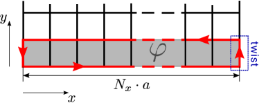
Figure 1: Flux of external field $\varphi$ through the stripe of plaquettes

Accounting for the periodicity of the lattice, the transformation (8) can be rewritten in the form of the TBC:

$$\left\{\begin{array}[]{l}U_{y}(N_{x},n_{y},n_{z},n_{t})=U_{y}(0,n_{y},n_{z},n_{t})\operatorname{e}^{i\varphi},\\ U_{\mu}(N_{x},n_{y},n_{z},n_{t})=U_{\mu}(0,n_{y},n_{z},n_{t}),\quad\mu\neq y,\\[10.00002pt] U_{\mu}(n_{x},N_{y},n_{z},n_{t})=U_{\mu}(n_{x},0,n_{z},n_{t}),\\ U_{\mu}(n_{x},n_{y},N_{z},n_{t})=U_{\mu}(n_{x},n_{y},0,n_{t}),\\ U_{\mu}(n_{x},n_{y},n_{z},N_{t})=U_{\mu}(n_{x},n_{x},n_{z},0).\end{array}\right.$$ (10)

In the present paper, the external Abelian field corresponding to the 3-rd Pauli matrix is introduced. For this case

$$\operatorname{e}^{i\varphi}=\operatorname{e}^{i\varphi_{3}\sigma_{3}/2}=\left(\begin{array}[]{cc}\operatorname{e}^{i\varphi_{3}/2}&0\\ 0&\operatorname{e}^{-i\varphi_{3}/2}\end{array}\right),$$ (11)

where $\sigma_{3}$ is the 3-rd Pauli matrix, $\varphi_{3}$ is the value of the applied flux. In the following the subscript of the $\varphi_{3}$ will be omitted.

3 Numerical Results

Let us investigate the influence of the external neutral Abelian field on the magnetic mass of the field, produced by the monopole-antimonopole string. The relevant quantity is the difference between the mean plaquettes in the presence and in the absence of the external field:

$$f(N)=|\langle U_{\mbox{\footnotesize field}}\rangle-\langle U_{0}\rangle|.$$ (12)

It is considered as a function of lattice size in spatial direction $N$. Lattices with symmetric spatial part are used here. The plaquettes are averaged over the lattice and over some number of simulation program runs (from 200 up to 1000 for various lattices).

There are several type behaviors of the quantity $f$ referred in the literature[10]: $f\sim 1/N^{2}$, when the magnetic flux tubes are formed and the flux is conserved; $f\sim 1/N^{4}$, corresponding to the Coulombic magnetic field, the flux decreases; $f\sim\operatorname{e}^{-kN^{2}}$, which means the screening of the field. In the last case $\sqrt{k}$ is the magnetic mass. From the investigation of the magnetic mass of the Abelian field [4], one more possible behavior of $f$ is known: $f\sim 1/N$. This corresponds to the increasing of the field flux due to, e.g., spontaneous field generation.

First of all, we are going to reproduce the results of the known investigation[10]. For the field produced by the monopole-antimonopole string the values $f(N)$ are obtained and fitted in order to determine, whether the applied field is screened or not. Then we add the external Abelian field flux and look how it changes the behavior of the quantity $f(N)$.

The MC simulations are performed on lattices $4\times N^{3}$ at three inverse couplings $\beta=2.835,\ 3.020,\ 3.091$, which correspond to the temperatures about 1.2, 1.9, 2.3 GeV. These temperatures are estimated using the relation[14]

$$T=T_{c}\,\frac{a(\beta_{c})}{a(\beta)},$$ (13)

where critical $\beta$ for the $4\times N^{3}$ lattices $\beta_{c}=2.301$ is found at $4\times 24^{3}$ lattice using the Polyakov loop susceptibility, $T_{c}=0.313$ GeV is taken from Ref. 15. Note that $\beta=3.020$ corresponds to the temperature used in Ref. 10 (in that case $\beta_{c}=1.8735$ is taken from Ref. 16).

The simulations are carried out with modification of the QCDGPU program [17] at GPUs of HybriLIT [18] cluster, HPCVillage [19] and HGPU Group [20] machines. In all the simulations the multihit heat-bath algorithm is used to update links, the number of hits is 10. Pseudorandom numbers are generated with RANLUX3 generator. Each program run includes 2000 thermalization sweeps and 1000 sweeps with measurements separated by 9 sweeps without measurements for decorrelation. The cold start is used. Calculations are performed with double precision.

The quantities $\langle U_{\mbox{\footnotesize field}}\rangle$ and $\langle U_{0}\rangle$ are calculated for each lattice size separately and combined into the quantity $f(N)$. To discern the functional dependence describing obtained data, they are linearized by logarithmization and fitted through minimization of $\chi^{2}$ function,

$$\chi^{2}(a)=\sum_{i=1}^{K}\frac{[y_{i}-\log f(N_{i};a)]^{2}}{\sigma_{i}^{2}},$$ (14)

where $y_{i}=\log f_{i}$, $f_{i}$ are the data for the quantity (12) obtained from simulations, $f(N;a)$ is a trial function, $K$ is the number of points used in fit, $a$ is a set of fitting parameters. The statistical errors $\sigma_{i}$ are estimated as for indirect measurement. Combinations of inverse power and exponential functions are tried in fit. To select which functions may describe data and which ones should be discarded, the $\chi^{2}$ criterion is used. The null hypothesis is that the trial function does describe the data, the alternate hypothesis is that it does not describe them. For each fit function the minimal value $\chi^{2}_{min}$ is calculated by Eq. 14 at estimated parameters $a$. This quantity is independent of the input parameters and follows the chi-squared distribution with $\nu$ degrees of freedom,

$$\nu=K-L,$$ (15)

where $L$ is the number of estimated parameters. Assuming that large values of $\chi^{2}_{min}$ are unlikely, it is compared with critical value of the chi-squared distribution $\chi^{2}_{\nu,0.05}$. If $\chi^{2}_{min}>\chi^{2}_{\nu,0.05}$, the null hypothesis is rejected. Here 0.05 is the probability of rejection of the true null hypothesis (type I error).

It can be shown that the difference

$$\Delta\chi^{2}=\chi^{2}(a)-\chi^{2}_{min}$$ (16)

is independent of the estimating and the input parameters and has the chi-squared distribution with $L$ degrees of freedom. Thus, the quantity (16) is compared with the critical value $\chi^{2}_{L,0.05}$, and the confidence intervals (CIs) for the parameters $a$ at 95% confidence level (CL) can be found from inequality

$$\chi^{2}(a)\leq\chi^{2}_{min}+\chi^{2}_{L,0.05}.$$ (17)

The data are presented in Fig. 3, the results of fitting are shown in Tables 3 – LABEL:KS:tab:fit_res0-3 for three considered temperatures. In all these tables the first columns contain trial fit functions, the second columns show the minimal $\chi^{2}$ values, the fourth columns contain threshold values $\chi^{2}_{\nu,0.05}$ for $\nu$ degrees of freedom listed in the third columns, then the conclusions from hypothesis testing are shown, and the last columns represent 95% CIs for parameters responsible for screening got from fit (dimensionless).

Fit results at $\varphi=0$, $\beta=2.835$    Function $\hskip 14.00003pt\chi^{2}_{min}$ $\nu$ $\chi^{2}_{\nu,0.05}$ Conclusion Estimate of $k$ with $2\sigma$ CI $A/N^{2}$ 80.4 4 9.49 rejected – $\left(A/N^{2}\right)\operatorname{e}^{-kN}$ 0.99 3 7.81 accepted $\left(3.95\pm 1.09\right)\times 10^{-1}$ $\left(A/N^{2}\right)\operatorname{e}^{-kN^{2}}$ 0.63 3 7.81 accepted $\left(2.30\pm 0.63\right)\times 10^{-2}$ $A/N^{4}$ 14.0 4 9.49 rejected – $\left(A/N^{4}\right)\operatorname{e}^{-kN}$ 2.32 3 7.81 accepted $(1.51\pm 1.09)\times 10^{-1}$ $\left(A/N^{4}\right)\operatorname{e}^{-kN^{2}}$ 1.36 3 7.81 accepted $(9.13\pm 6.29)\times 10^{-3}$ $A\operatorname{e}^{-kN}$ 0.40 3 7.81 accepted $(6.39\pm 1.09)\times 10^{-1}$ $A\operatorname{e}^{-kN^{2}}$ 3.18 3 7.81 accepted $(3.68\pm 0.63)\times 10^{-2}$ $A/N$ 137 4 9.49 rejected – $(A/N)\operatorname{e}^{-kN}$ 0.60 3 7.81 accepted $(5.17\pm 1.09)\times 10^{-1}$ $(A/N)\operatorname{e}^{-kN^{2}}$ 1.49 3 7.81 accepted $(2.99\pm 0.63)\times 10^{-2}$

Fit results at $\varphi=0$, $\beta=3.020$

Figure 2: (top) Contributions of the external field to the average plaquette in the cases of absence (open markers) and presence (filled markers) of the additional Abelian field flux; (bottom) logarithms of these contributions. The bins represent standard deviations for the measured quantities. For $\beta=3.020$ and $\beta=3.091$ data are shifted to the right for better visibility.

Fit results at $\varphi=0.08$, $\beta=2.835$    Function $\hskip 1.75pt\chi^{2}_{min}$ $\hskip 0.06996pt\nu$ $\hskip 1.75pt\chi^{2}_{\nu,0.05}$ Conclusion Estimate of parameters with $2\sigma$ CI $A/N^{b}$ 91.2 9 16.9 rejected $b=1.65\pm 0.10$ $(A/N^{b})\operatorname{e}^{-kN}$ 30.0 8 15.5 rejected $b=2.59\pm 0.35$ $k=(-4.59\pm 1.63)\times 10^{-2}$ $(A/N^{b})\operatorname{e}^{-kN^{2}}$ 47.2 8 15.5 rejected $b=2.07\pm 0.20$ $k=(-3.45\pm 1.43)\times 10^{-4}$ $A\operatorname{e}^{B/N}\operatorname{e}^{-kN}$ 5.33 8 15.5 accepted $B=20.3\pm 2.64$ $k=(1.09\pm 0.91)\times 10^{-2}$

Fit results at $\varphi=0.08$, $\beta=3.020$    Function $\hskip 1.75pt\chi^{2}_{min}$ $\hskip 0.06996pt\nu$ $\hskip 1.75pt\chi^{2}_{\nu,0.05}$ Conclusion Estimate of parameters with $2\sigma$ CI $A/N^{b}$ 170 8 15.5 rejected $b=1.71\pm 0.07$ $(A/N^{b})\operatorname{e}^{-kN}$ 44.9 7 14.1 rejected $b=2.65\pm 0.24$ $k=(-5.22\pm 1.29)\times 10^{-2}$ $(A/N^{b})\operatorname{e}^{-kN^{2}}$ 73.7 7 14.1 rejected $b=2.11\pm 0.14$ $k=(-4.44\pm 1.25)\times 10^{-4}$ $A\operatorname{e}^{B/N}\operatorname{e}^{-kN}$ 7.14 7 14.1 accepted $B=20.1\pm 1.84$ $k=(1.08\pm 0.75)\times 10^{-2}$

Fit results at $\varphi=0.08$, $\beta=3.091$    Function $\hskip 1.75pt\chi^{2}_{min}$ $\hskip 0.06996pt\nu$ $\hskip 1.75pt\chi^{2}_{\nu,0.05}$ Conclusion Estimate of parameters with $2\sigma$ CI $A/N^{b}$ 223 10 18.3 rejected $b=1.56\pm 0.08$ $(A/N^{b})\operatorname{e}^{-kN}$ 69.0 9 16.9 rejected $b=2.67\pm 0.26$ $k=(-5.55\pm 1.23)\times 10^{-2}$ $(A/N^{b})\operatorname{e}^{-kN^{2}}$ 118 9 16.9 rejected $b=2.02\pm 0.15$ $k=(-4.30\pm 1.16)\times 10^{-4}$ $A\operatorname{e}^{B/N}\operatorname{e}^{-kN}$ 7.00 9 16.9 accepted $B=21.3\pm 2.01$ $k=(6.90\pm 6.76)\times 10^{-3}$

As it is seen from the tables, for all three temperatures the first three trial functions are rejected at 95% CL. The last behavior is accepted at this CL. In the correspondent function

$$f=A\operatorname{e}^{B/N}\operatorname{e}^{-kN}$$ (18)

the parameter $k$ serves as magnetic mass, while $B$ is some “enhancing” parameter. Passing to the physical units, one can see that the parameter

$$B_{phys}=a\cdot B$$ (19)

decreases with temperature, while the magnetic mass

$$m_{magn}=k/a$$ (20)

is constant within CIs at the considered range of temperatures (see Fig. 3); $a$ is lattice spacing. Averaging over three used temperatures one obtains the magnetic mass $(1.83\pm 0.87)\times 10^{-2}$ GeV at 95% CL.

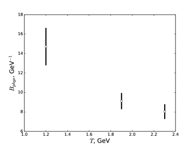
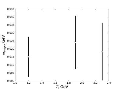
Figure 3: Quantities $B_{phys}$ and $m_{magn}$ as functions of temperature. Bars correspond to 95% CIs.

To compare the obtained magnetic mass values with the ones corresponding to the absence of the additional Abelian flux, the data at $\varphi=0$ are fitted with the trial function (18). The results of this fit are shown in Table 3. The first line represents minimal $\chi^{2}$ values. Comparison of them with $\chi^{2}_{\nu;0.05}=5.99$ shows that the function (18) describes data correctly at 95% CL for all three temperatures. The last two rows contain the estimates and CIs for the dimensionless parameters $B$ and $k$. The averaged over considered temperatures magnetic mass is $1.26\pm 0.41$ GeV.

Fit results at $\varphi=0$ with $f=A\operatorname{e}^{B/N}\operatorname{e}^{-kN}$. For all temperatures $\nu=2$, $\chi^{2}_{\nu;0.05}=5.99$ $\beta=2.835$ $\beta=3.020$ $\beta=3.091$ $\chi^{2}_{min}$ 0.36 1.34 0.64 $\hat{B}\pm 2\sigma$ CI $-2.81\pm 37.6$ $-4.95\pm 14.2$ $5.04\pm 23.9$ $\hat{k}\pm 2\sigma$ CI $(6.83\pm 5.76)\times 10^{-1}$ $(6.29\pm 2.46)\times 10^{-1}$ $(4.92\pm 3.66)\times 10^{-1}$

Hence it is seen that the magnetic mass of the chromomagnetic field produced by monopole-antimonopole string in the presence of the external Abelian field flux is two orders of magnitude less than the magnetic mass of solely monopole-antimonopole string field. This means that the magnetic mass of the neutral Abelian field is much smaller than the magnetic mass of the color charged components.

Let us discuss this in more details. To simplify situation we propose that the first field flux produced by the string through one plaquette is described by the function $e^{-aN}$ and for the second one generated by TBC it is $e^{-bN}$, $a$ and $b$ are corresponding magnetic masses. The magnetic mass of the total flux is defined from the function $e^{-cN}$. Hence, independently of the chosen prefactors, the relation holds

$$e^{-aN}+e^{-bN}=2e^{-cN}.$$ (21)

It follows from the flux conservation. Assuming the masses are small, it is easily to get the relation $c=\sqrt{ab}$. To have $c$ two order less than $a$ the mass $b$ has to be of the order $b\sim a^{5}$. That is the magnetic mass of the Abelian magnetic field must be negligibly small and dominant in the total flux. This conclusion is in agreement with the results of Refs. 22, 23, 24, 4 obtained in analytic and MC calculations, that this mass is zero. Thus, there is no static screening effect for such type fields. This fact is similar to the one for usual static magnetic field in QED plasma.

4 Conclusions and Discussion

To investigate the SU(2) structure of the magnetic mass, the influence of the external Abelian neutral chromomagnetic field on the field of monopole-antimonopole string was investigated by the methods of lattice gluodynamics.

First we convinced that in the absence of the external Abelian field the results of Ref. 10 are reproduced. We have obtained that the field of the monopole-antimonopole string is screened. When the external neutral Abelian field flux is added, the character of screening is changed drastically. It was found that it is not described by just a one decreasing exponent anymore. The extra factor corresponding to “enhancement” behavior appears. This factor decreases with temperature increases, whereas the magnetic mass turns out to be two order less than at zero Abelian flux and constant for all the range of considered temperatures.

Appearance of the “enhancing” factor demonstrates (independently of Ref. 4) that magnetic mass of the Abelian field is zero with high accuracy possible in numeric calculations. Moreover, the magnetic flux passing through a plaquette is grater compared to the zero field case. This also means that Abelian field occupies whole the volume of the lattice. On the contrary, the non-Abelian field is screened, and it may be observed just up to distances of the order of the inverse magnetic mass in Eq. (1). Thus, as a conclusion, the Abelian magnetic fields only have to be present in the volume of QGP. To investigate in detail the analytic field and temperature dependence of $m_{magn}(H,T)$ one has to consider a model with more then one elements in the center of the group. This is a subject for further investigation.

The absence of the static screening for Abelian magnetic fields resembles the case of magnetic fields in QED. In gluodynamics, it has also been detected already in analytic [22, 23, 24] and lattice [4] calculations. This is in contrast to the Debye mass. In the field presence the mass is (in high temperature approximation)[22]:

$$m^{2}_{D}(H,T)=\frac{2}{3}T^{2}\left[1-0.8859\left(\frac{\sqrt{gH}}{2T}\right)+O((gH)^{2}/T^{4})\right].$$ (22)

Its value is decreased compared to the zero field case. Thus, chromoelectric static fields become more long range ones.

However, such a situation does not exclude a dynamical screening and gap for gluon modes. It can happen for nonzero momentum $k_{4}\not=0$. In QGP under influence of strong magnetic fields, it was investigated recently in Ref. 25 on the base of Schwinger-Dyson’s equation for gluon fields.

The Abelian field was introduced on the lattice through the TBC. Despite this field is not gauge invariant, it is the solution to the Yang-Mills field equations without sources. Just such type solutions can be realized spontaneously in nature. How to deal with the non-gauge invariant solutions to obtain a gauge invariant vacuum has been discussed by Feynman [26]. He noted that to find a gauge invariant vacuum one should select a contour in space-time which saplies a gauge invariant integral for a chosen field potential. Such procedure leads to the vacuum domain structure. The form of the lattice can be obtained from the requirements of gauge invariance for phase integral over lattice contour and lowering the free energy of this configuration. Thus, it is expected the lattice vacuum structure of QGP. In fact, it is not difficult to investigate such a structure on the lattice and this is also the problem for the future.

Acknowledgments

The authors are grateful to Alexey V. Gulov for useful discussions and careful reading the manuscript. One of us would like to thank the HybriLIT of JINR, HPC Village project and HGPU group for the computational resources provided.

References

- [1] Y. Aoki, S. Borsanyi, S. Durr, Z. Fodor, S. D. Katz, S. Krieg and K. K. Szabo, JHEP 06, 088 (2009), arXiv:0903.4155 [hep-lat], 10.1088/1126-6708/2009/06/088.
- [2] D. J. Gross, R. D. Pisarski and L. G. Yaffe, Rev. Mod. Phys. 53, 43 (1981), 10.1103/RevModPhys.53.43.
- [3] M. Bordag and V. Skalozub, Phys. Rev. D85, 065018 (2012), arXiv:1201.1978 [hep-th], 10.1103/PhysRevD.85.065018.
- [4] S. Antropov, M. Bordag, V. Demchik and V. Skalozub, Int. J. Mod. Phys. A26, 4831 (2011), arXiv:1011.3147 [hep-ph], 10.1142/S0217751X11054747.
- [5] V. Skalozub and M. Bordag, Nucl. Phys. B576, 430 (2000), arXiv:hep-ph/9905302 [hep-ph], 10.1016/S0550-3213(00)00101-2.
- [6] V. V. Skalozub and A. V. Strelchenko, Eur. Phys. J. C33, 105 (2004), arXiv:hep-ph/0208071 [hep-ph], 10.1140/epjc/s2003-01577-5.
- [7] V. Skalozub and P. Minaev, Phys. Part. Nucl. Lett. 15, 568 (2018), arXiv:1708.02792 [hep-ph], 10.1134/S1547477118060171.
- [8] P. Cea and L. Cosmai, Phys. Rev. D60, 094506 (1999), arXiv:hep-lat/9903005 [hep-lat], 10.1103/PhysRevD.60.094506.
- [9] P. Cea and L. Cosmai (2001), arXiv:hep-lat/0101017 [hep-lat].
- [10] T. A. DeGrand and D. Toussaint, Phys. Rev. D25, 526 (1982), 10.1103/PhysRevD.25.526.
- [11] C. Gattringer and C. B. Lang, Lect. Notes Phys. 788, 1 (2010), 10.1007/978-3-642-01850-3.
- [12] M. Srednicki and L. Susskind, Nucl. Phys. B179, 239 (1981), 10.1016/0550-3213(81)90237-6.
- [13] M. Vettorazzo and P. de Forcrand, Nucl. Phys. B686, 85 (2004), arXiv:hep-lat/0311006 [hep-lat], 10.1016/j.nuclphysb.2004.02.038.
- [14] N. Cardoso and P. Bicudo, Phys. Rev. D85, 077501 (2012), arXiv:1111.1317 [hep-lat], 10.1103/PhysRevD.85.077501.
- [15] P. V. Buividovich, M. N. Chernodub, E. V. Luschevskaya and M. I. Polikarpov, Nucl. Phys. B826, 313 (2010), arXiv:0906.0488 [hep-lat], 10.1016/j.nuclphysb.2009.10.008.
- [16] A. Velytsky, Int. J. Mod. Phys. C19, 1079 (2008), arXiv:0711.0748 [hep-lat], 10.1142/S0129183108012741.
- [17] V. Demchik and N. Kolomoyets, Comp. Sci. and App. 1, 13 (2014), arXiv:1310.7087 [hep-lat], https://github.com/vadimdi/QCDGPU (Last access: Jan. 2018).
- [18] http://hlit.jinr.ru/, (Last access: Aug. 2018).
- [19] http://openwall.info/wiki/HPC/Village, (Last access: Aug. 2018).
- [20] https://hgpu.org/, (Last access: Aug. 2018).
- [21] S. Necco and R. Sommer, Nucl. Phys. B622, 328 (2002), arXiv:hep-lat/0108008 [hep-lat], 10.1016/S0550-3213(01)00582-X.
- [22] M. Bordag and V. Skalozub, Phys. Rev. D75, 125003 (2007), arXiv:hep-th/0611256 [hep-th], 10.1103/PhysRevD.75.125003.
- [23] M. Bordag and V. Skalozub, Phys. Rev. D77, 105013 (2008), arXiv:0801.2306 [hep-th], 10.1103/PhysRevD.77.105013.
- [24] V. V. Skalozub and A. V. Strelchenko, Eur. Phys. J. C40, 121 (2005), arXiv:hep-ph/0408030 [hep-ph], 10.1140/epjc/s2005-02106-4.
- [25] K. Hattori and D. Satow, Phys. Rev. D97, 014023 (2018), arXiv:1704.03191 [hep-ph], 10.1103/PhysRevD.97.014023.
- [26] R. P. Feynman, Nucl. Phys. B188, 479 (1981).