Dynamical quantum phase transitions in discrete time crystals

Abstract

Discrete time crystals are related to non-equilibrium dynamics of periodically driven quantum many-body systems where the discrete time translation symmetry of the Hamiltonian is spontaneously broken into another discrete symmetry. Recently, the concept of phase transitions has been extended to non-equilibrium dynamics of time-independent systems induced by a quantum quench, i.e. a sudden change of some parameter of the Hamiltonian. There, the return probability of a system to the ground state reveals singularities in time which are dubbed dynamical quantum phase transitions. We show that the quantum quench in a discrete time crystal leads to dynamical quantum phase transitions where the return probability of a periodically driven system to a Floquet eigenstate before the quench reveals singularities in time. It indicates that dynamical quantum phase transitions are not restricted to time-independent systems and can be also observed in systems that are periodically driven. We discuss how the phenomenon can be observed in ultra-cold atomic gases.

I Introduction

Phase transitions in equilibrium statistical physics are related to abrupt changes of macroscopic properties of many-body systems Sachdev (2011); Sachdev and Keimer (2011). Macroscopic quantities that characterize systems in the thermodynamic limit reveal non-analytical behavior as a function of a control parameter. The equilibrium phase transitions are much better understood than non-equilibrium dynamics of quantum many-body systems Eckstein et al. (2009); Garrahan and Lesanovsky (2010); Diehl et al. (2010); Schiró and Fabrizio (2010); Sciolla and Biroli (2010, 2011); Ates et al. (2012); Sciolla and Biroli (2013); Vosk and Altman (2014); Žunkovič et al. (2016); Maraga et al. (2016). Recently, it has been shown that real-time evolution of time-independent many-body systems, after a quantum quench, can reveal non-analytical behavior at a critical time Heyl et al. (2013); Heyl (2015); Budich and Heyl (2016); Sharma et al. (2016); Bhattacharya and Dutta (2017); Bhattacharya et al. (2017); Karrasch and Schuricht (2017); Heyl and Budich (2017); Halimeh and Zauner-Stauber (2017); Zauner-Stauber and Halimeh (2017); Homrighausen et al. (2017); Lang et al. (2017); Zunkovic et al. (2016). That is, starting with a system in the ground state, a sudden change of some parameter of the Hamiltonian results in non-analytical evolution of the return probability to the initial ground state. This phenomenon has been termed dynamical quantum phase transition and it has been already demonstrated in experiments Fläschner et al. (2016); Jurcevic et al. (2017), for review see Heyl (2017).

In 2012 Frank Wilczek suggested that periodic structures in time could be formed spontaneously by a quantum many-body system Wilczek (2012). The original idea of such a time crystal could not be realized because it assumed a system in the ground state Bruno (2013); Watanabe and Oshikawa (2015); Syrwid et al. (2017); Iemini et al. (2017); Huang et al. (2017a); Prokof’ev and Svistunov (2017). However, soon it turned out that periodically driven quantum many-body systems were able to self-re-organize their motion and spontaneously start evolving with a period which was different than a period of an external driving Sacha (2015a); Khemani et al. (2016); Else et al. (2016); Yao et al. (2017); Lazarides and Moessner (2017); Russomanno et al. (2017); Zeng and Sheng (2017); Nakatsugawa et al. (2017); Ho et al. (2017); Huang et al. (2017b); Gong et al. (2017); Wang et al. (2017). These quantum phenomena are dubbed discrete time crystals because discrete time translation symmetry is broken into another discrete symmetry. Discrete time crystals have been recently observed experimentally Zhang et al. (2017); Choi et al. (2017); Nayak (2017). It should be stressed that in the classical regime breaking of discrete time translation symmetry in an atomic system has been also demonstrated in a laboratory Kim et al. (2006); Heo et al. (2010). Wilczek idea initiated a new research area where non-trivial crystalline structures are investigated in the time domain Guo et al. (2013); Sacha (2015b); Sacha and Delande (2016); Guo and Marthaler (2016); Guo et al. (2016); Giergiel and Sacha (2017); Mierzejewski et al. (2017); Delande et al. (2017); Flicker (2017); Liang et al. (2017); Giergiel et al. (2017), for review see Sacha and Zakrzewski (2018).

Discrete time crystal formation takes place if interactions between particles are sufficiently strong. If they are not, exact many-body Floquet eigenstates evolve with a period of an external driving and are not vulnerable to infinitesimally weak perturbations. However, when the strength of particle interactions is greater than a critical value, Floquet eigenstates possess Schrödinger cat like structures and any perturbation, or even measurement of a position of a single particle, has a dramatic effect on system dynamics leading to a change of the period of motion Sacha (2015a); Sacha and Zakrzewski (2018). Here we will show that starting with a Floquet eigenstate in the regime of time crystal formation, an abrupt change of the particle interaction strength to the weak interaction regime induces dynamical quantum phase transitions. That is, the return probability to the initial Floquet eigenstate reveals singularities in time. In the second part of the article we consider singularities in the dynamics of states with spontaneously broken time translation symmetry, and identify experimentally measurable observables.

II Results

We will focus on the discrete time crystal described in Ref. Sacha (2015a), i.e. on ultra-cold bosonic atoms bouncing on a harmonically oscillating (with frequency $\omega$) mirror in the presence of the gravitational force Steane et al. (1995); Lau et al. (1999); Bongs et al. (1999); Buchleitner et al. (2002). Let us begin with a single particle problem. In the frame moving with the mirror and in the gravitational units the Hamiltonian for a single-particle system reads $H_{0}=\frac{p^{2}}{2}+x+\Lambda x\cos(\omega t)$ where $x\geq 0$, i.e. the mirror is located at $x=0$ in the moving frame, and $\frac{\Lambda}{\omega^{2}}$ is the amplitude of the mirror oscillations in the laboratory frame Buchleitner et al. (2002). Classical description of a single particle reveals resonant periodic orbits with periods equal to integer multiples of the driving period $\frac{2\pi}{\omega}$. We will concentrate on the 2:1 resonance where the classical resonant orbit possesses the period $2\frac{2\pi}{\omega}$. In the quantum description there exist two Floquet eigenstates which are represented by two orthogonal superpositions, $u_{1,2}(x,t)\propto\phi_{1}\pm\phi_{2}$, of two localized wavepackets, $\phi_{1,2}(x,t)$, that move along the 2:1 resonant orbit like a classical particle. Each of these two wavepackets evolves with the period $2\frac{2\pi}{\omega}$ but because after every period $\frac{2\pi}{\omega}$ they exchange their roles, the Floquet eigenstates $u_{1,2}$ are periodic with the period of the external driving. The two Floquet states are eigenstates of the single particle Floquet Hamiltonian, $(H_{0}-i\partial_{t})u_{1,2}=\varepsilon_{1,2}u_{1,2}$, corresponding to quasi-energies $\varepsilon_{2}=\varepsilon_{1}+J$ (modulo $\frac{\omega}{2}$) where $J$ is an amplitude related to tunneling of a particle from one of the wavepacket to the other one.

In order to find many-body Floquet eigenstates for ultra-cold atoms bouncing on the oscillating mirror we assume that interaction energy per particle is much smaller than the energy gap for excitation of the localized wavepackets. In the following we use the parameters as in Ref. Sacha (2015a), i.e. $\Lambda=0.06$ and $\omega=1.1$, then the energy gap is about $10^{3}J$ while the interaction energy we consider is of the order of $10J$. Therefore, we may restrict to the consideration of behavior of the $N$-body system in the Hilbert subspace spanned by Fock states $|N-n,n\rangle$ where $N-n$ and $n$ are occupations of the localized wavepackets $\phi_{1}$ and $\phi_{2}$, respectively Sacha (2015a, b). This approximation resembles the two-mode approximation known in the description of a many-body system in a double-well potential Raghavan et al. (1999). In the time-dependent two-mode basis $\{\phi_{1}(x,t),\phi_{2}(x,t)\}$, our $N$-body Floquet Hamiltonian reduces to

$$\hat{H} = -\frac{J}{2}(\hat{a}_{1}^{\dagger}\hat{a}_{2}+\hat{a}_{2}^{\dagger}\hat{a}_{1})+\frac{U}{2}(\hat{a}_{1}^{\dagger}\hat{a}_{1}^{\dagger}\hat{a}_{1}\hat{a}_{1}+\hat{a}_{2}^{\dagger}\hat{a}_{2}^{\dagger}\hat{a}_{2}\hat{a}_{2})$$ (2)

$$+2U_{12}\hat{a}_{1}^{\dagger}\hat{a}_{1}\hat{a}_{2}^{\dagger}\hat{a}_{2},$$

where the standard bosonic operators $\hat{a}_{1,2}$ annihilate particles in the modes $\phi_{1,2}$, $U=g_{0}\int_{0}^{4\pi/\omega}dt\int_{0}^{\infty}dx|\phi_{1,2}|^{4}$ and $U_{12}=g_{0}\int_{0}^{4\pi/\omega}dt\int_{0}^{\infty}dx|\phi_{1}|^{2}|\phi_{2}|^{2}$ with $g_{0}$ determined by $s$-wave scattering length of atoms Sacha (2015a). For very weak interactions, i.e. for $\gamma=N(U-2U_{12})/J\approx 0$, the ground state of the Hamiltonian (2) corresponds to a Bose-Einstein condensate where all bosons occupy the single particle Floquet state $u_{1}(x,t)$. However, if particle interactions are attractive ($g_{0}<0$) and sufficiently strong, $\gamma\ll-1$, it is energetically favorable to group all atoms in one of the localized wavepackets. Then, for large $N$, low-lying eigenstates of the Hamiltonian (2) are dominated by pairs of nearly degenerate Schrödinger cat like states Ziń et al. (2008); Oleś et al. (2010). For example, the lowest two eigenstates of (2) are $|\psi_{\pm}(t)\rangle\approx(|N,0\rangle\pm|0,N\rangle)/\sqrt{2}$. Such many-body Floquet eigenstates evolve with the period of the external driving $\frac{2\pi}{\omega}$. However, even if the many-body system is prepared initially in one of such Schrödinger cat like states, e.g. in the Floquet eigenstate $|\psi_{+}\rangle$, measurement of a position of a single particle leads to a collapse of the eigenstate to $|N,0\rangle$ or $|0,N\rangle$ state what breaks the original time translation symmetry because the subsequent time evolution takes place with the period $2\frac{2\pi}{\omega}$ Sacha (2015a). The lifetime of the symmetry broken state goes to infinity when $N\rightarrow\infty$ but $\gamma=$constant.

In the first part of this article we do not consider spontaneous breaking of time translation symmetry but we assume that the perfectly isolated system is prepared in the Floquet eigenstate $|\psi_{+}(t)\rangle=K(t,0)|\psi_{+}(0)\rangle$, where $K(t,0)$ is the time evolution operator corresponding to $\gamma<-1$ and $|\psi_{+}(0)\rangle$ is the Floquet eigenstate at $t=0$. Subsequently, we assume that at $t=t_{0}>0$ the $s$-wave scattering length $g_{0}$ is suddenly changed to, e.g., zero. After the quench, the state evolves according to the new time evolution operator: $|\tilde{\psi}_{+}(t)\rangle=\tilde{K}(t,t_{0})|\psi_{+}(t_{0})\rangle$. Time evolution of $|\tilde{\psi}_{+}(t)\rangle$ can be easily obtained by numerical integration of the many-body Schrödinger equation with the Hamiltonian (2) (this Hamiltonian can be rewritten in the form of the spin system Hamiltonian Milburn et al. (1997) or the infinite-range Ising model Žunkovič et al. (2016)). However, it is much more instructive to apply the so-called continuum approximation Ziń et al. (2008) which reduces the many-body Hamiltonian (2) to the Hamiltonian of a fictitious particle,

$$\hat{H}=-\frac{J}{N}\sqrt{1-z^{2}}\frac{\partial^{2}}{\partial{z^{2}}}+V(z),$$ (3)

in the presence of the effective potential,

$$V(z)=\frac{JN}{2}\left(-\sqrt{1-z^{2}}+\frac{\gamma}{2}z^{2}\right).$$ (4)

Wavefunction $\psi(z)$ of the fictitious particle is a many-body state written in the Fock space basis $|N-n,n\rangle$ but with the assumption that number of particles $N$ is so large that the relative population difference $z_{n}=\frac{(N-n)-n}{N}$ can be treated as a continuous variable $z$ with the restriction $|z|\leq 1$.

There are two crucial ranges of the parameter $\gamma$. For $\gamma<-1$ the effective potential (4) possesses a double well structure, while for $\gamma>-1$ it has a single well shape Ziń et al. (2008). For $\gamma<-1$, the ground state of the fictitious particle can be approximated by the superposition $\psi_{+}(z)=[\psi_{L}(z)+\psi_{R}(z)]/\sqrt{2}$, where $\psi_{L,R}$ are Gaussian states. (See the Appendix A for a derivation of the continuum approximation, and the analytical solutions for $|\tilde{\psi}_{+}(t)\rangle$.) The state $\psi_{+}(z)$ is the previously described $N$-body Floquet eigenstate $|\psi_{+}(t)\rangle=\sum_{n}\psi_{+}(z_{n})|N-n,n\rangle$ written in the time-dependent Fock basis and within the continuum approximation.

Let us assume that the system is prepared in the ground state $\psi(z)=\psi_{+}(z)$ of the Hamiltonian (3) for $\gamma<-1$ and at $t=t_{0}$ we suddenly set the scattering length $g_{0}$ to zero, i.e. we switch to $\gamma=0$. The state $\tilde{\psi}(z,t>t_{0})$ evolves according to the new Hamiltonian and we are interesting in the so-called Loschmidt echo Heyl et al. (2013), i.e. the return probability to the initial state, $|{\cal G}(t>t_{0})|^{2}$, where ${\cal G}(t)=\int_{-1}^{1}dz\psi^{*}_{+}(z)\tilde{\psi}(z,t)$. Such a Loschmidt echo corresponds actually to the return probability of the evolving $N$-body state $|\tilde{\psi}_{+}(t)\rangle=\sum_{n}\tilde{\psi}(z_{n},t>t_{0})|N-n,n\rangle$ to the time-periodic Floquet eigenstate $|\psi_{+}(t)\rangle$, i.e. ${\cal G}(t>t_{0})=\langle\psi_{+}(t)|\tilde{\psi}_{+}(t)\rangle$. The Floquet eigenstate $|\psi_{+}(t)\rangle$ evolves periodically in time with the period $\frac{2\pi}{\omega}$ (modulo time-dependent global phase). The state $|\tilde{\psi}_{+}(t)\rangle$ also reveals nearly periodic behavior on short time intervals around any $t$, however, it becomes very quickly nearly orthogonal to $|\psi_{+}(t)\rangle$ if $N$ is large. Dynamical quantum phase transitions are associated with non-analytic behavior of the Loschmidt echo $|{\cal G}(t>t_{0})|^{2}$. In order to study the quantum phase transitions in time, it is convenient to define an intensive rate function

$$\lambda_{+}(t)=\lim\limits_{N\rightarrow\infty}\lambda_{+}^{(N)}(t),\quad\lambda_{+}^{(N)}=-N^{-1}\ln|{\cal G}(t)|^{2}.$$ (5)

In Fig. 1(a) we show the rate function $\lambda_{+}^{(N)}(t)$ obtained analytically within the continuum approximation, i.e. starting with $\psi(z,t_{0})=[\psi_{L}(z)+\psi_{R}(z)]/\sqrt{2}$ for $\gamma=-1.15$ and $N=1500$ we obtain subsequent evolution of $\tilde{\psi}(z,t>t_{0})$ for $\gamma=0$ by harmonic approximation of the potential (4) and by dropping $\sqrt{1-z^{2}}$ in (3). (See Appendix A for the derivation of the rate function $\lambda_{+}(t)$.) The analytical results follow closely the results of the full numerical integration of the $N$-body Schrödinger equation (also shown in Fig. 1) and allow us to obtain $\lambda_{+}^{(N)}(t)$ in regimes where the Loschmidt echo is so small that the numerical precision breaks down. Cusp-like non-analytic behavior of $\lambda_{+}(t)$ appear at critical times $t_{c}=t_{0}+\frac{\pi}{2J}$ (modulo $\frac{\pi}{J}$). That is, one can show that $\frac{d}{dt}\lambda_{+}(t)$ is discontinuous,

$$\lim\limits_{t\rightarrow t_{c}^{\pm}}\frac{d\lambda_{+}(t)}{dt}=\lim\limits_{t\rightarrow t_{c}^{\pm}}\lim\limits_{N\rightarrow\infty}\frac{d\lambda_{+}^{(N)}(t)}{dt}=\mp\frac{2q^{2}\Omega^{3}}{(1+\Omega^{2})^{2}},$$ (6)

where $\Omega=\sqrt{\gamma(1-\gamma^{2})}(1-q^{2})^{-1/4}$. It should be stressed that the order of the limits is important. Indeed, $\lim\limits_{t\rightarrow t_{c}}\lambda_{+}(t)$ is well defined but

$$\lim\limits_{N\rightarrow\infty}\lambda_{+}^{(N)}(t_{c})=\frac{q^{2}\Omega}{1+\Omega^{2}}-\lim_{N\rightarrow\infty}\frac{1}{N}\ln\left[\cos^{2}\left(\frac{Nq^{2}\Omega^{2}}{2(1+\Omega^{2})}\right)\right],$$ (7)

is not because whenever the cosine in (7) is close to zero, the logarithm diverges which corresponds to accidental values of $N$ for which the Loschmidt echo vanishes. In Fig. 1(b) we show $\lambda_{+}^{(N)}(t)$ around the first critical moment of time for different $N$. With the increasing particle number we get closer to the non-analytical behavior but for some specific values of $N$ the rate diverges.

The Loschmidt echo can be interpreted as information about the evolving system from the point of view of the initial Floquet eigenstate. At the critical time we are not able to extrapolate such information because of the breakdown of a short time expansion. Hilbert space of the system is spanned by the Fock states $|n_{1},n_{2}\rangle$ where only two modes $\phi_{1,2}(x,t)$ are occupied by particles. It turns out that not only the Loschmidt echo but also the von Neumann entropy of the reduced density matrix of the system after the quench, i.e. $S(t>t_{0})=-\mbox{tr}\left(\rho_{1}\ln\rho_{1}\right)$ where $\rho_{1}=\sum_{n_{2}}\langle n_{2}|\tilde{\psi}_{+}(t)\rangle\langle\tilde{\psi}_{+}(t)|n_{2}\rangle$, reveals non-analytical behavior at critical moments of times. Indeed, within the continuum approximation $S(t)=-\sum_{n}|\tilde{\psi}(z_{n},t)|^{2}\ln|\tilde{\psi}(z_{n},t)|^{2}$ and

$$\lim\limits_{t\rightarrow t_{c}^{\pm}}\left[S(t)-S(t_{c})\right]\approx 1.$$ (8)

Figure 2 illustrates such a sudden jump of the entropy in the system of $N=10^{4}$ particles, see Appendix B.

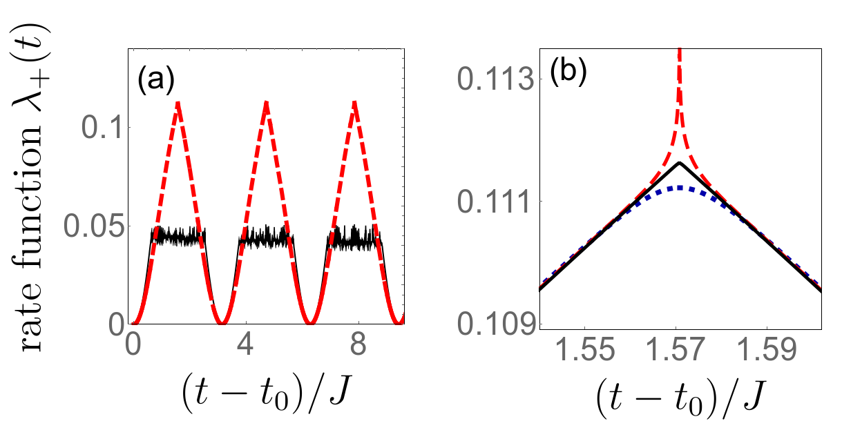
Figure 1: Quench from $\gamma=-1.15$ to $\gamma=0$ in the system prepared initially in the Floquet state $|\psi_{+}(t)\rangle$. Panel (a): the rate function $\lambda_{+}^{(N)}(t)$ obtained numerically (solid black line) and analytically within the continuum approximation (red dashed line) for $N=1500$. Both curves follow each other except time intervals when the Loschmidt echo is so small that the numerical precision breaks down. Panel (b): rate function $\lambda_{+}^{(N)}(t)$ for $N=$2000 (blue dotted), 4869 (red dashed) and 50000 (black solid) in the vicinity of the critical time $t_{c}=t_{0}+\frac{\pi}{2J}$. The diverging curve is related to an accidental value of $N$ when the Loschmidt echo vanishes, cf. (7).

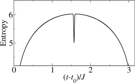
Figure 2: Quench from $\gamma=-50$ to $\gamma=0$ in the system of $N=10^{4}$ particles prepared initially in the Floquet state $|\psi_{+}(t)\rangle$. Figure shows von Neumann entropy of the reduced density matrix of the system, i.e. $S(t>t_{0})=-\mbox{tr}\left(\rho_{1}\ln\rho_{1}\right)$ where $\rho_{1}=\sum_{n_{2}}\langle n_{2}|\tilde{\psi}_{+}(t)\rangle\langle\tilde{\psi}_{+}(t)|n_{2}\rangle$, after the quench. The results are obtained by numerical integration of the $N$-body Schrödinger equation. The jump of the entropy visible around the critical moment of time is consistent with Eq. (8).

So far we have considered the system prepared initially in the Floquet state $|\psi_{+}(t)\rangle$ that corresponds to the ground state of the Hamiltonian (2) – within the continuum approximation $\psi_{+}(z)=[\psi_{L}(z)+\psi_{R}(z)]/\sqrt{2}$. The first excited eigenstate of (2) can be approximated by $\psi_{-}(z)=[\psi_{L}(z)-\psi_{R}(z)]/\sqrt{2}$ and its eigenenergy becomes degenerate with the ground state energy when $N\rightarrow\infty$. If $\gamma\ll-1$, the Floquet state $|\psi_{+}(t)\rangle$ is actually a Schrödinger cat-like state and it could be very difficult to prepare it experimentally because any loss of atoms makes the Schrödinger cat collapse to one of the states $|\psi_{L,R}(t)\rangle$ Sacha (2015a). Assume, that for $\gamma\ll-1$ we have prepared the system in the state $|\psi(t)\rangle=|\psi_{R}(t)\rangle=[|\psi_{+}(t)-|\psi_{-}(t)\rangle]/\sqrt{2}$ which is a symmetry broken state because it evolves with the period twice longer than $\frac{2\pi}{\omega}$ Sacha (2015a). At $t=t_{0}$ we switch the scattering length $g_{0}$ to zero. If the ground state level of the initial Hamiltonian is degenerate, the Loschmidt echo is generalized to the return probability of the state after the quench to the ground state manifold Heyl et al. (2013); Zunkovic et al. (2016), i.e.

$${\cal P}(t>t_{0})=|{\cal G}_{L}(t)|^{2}+|{\cal G}_{R}(t)|^{2}$$ (9)

where ${\cal G}_{L,R}(t)=\langle\psi_{L,R}(t)|\tilde{\psi}(t)\rangle$. The rate function of the return probability reads

$$\lambda(t)=-\lim\limits_{N\rightarrow\infty}N^{-1}\ln[{\cal P}(t)]={\rm min}[\lambda_{L}(t),\lambda_{R}(t)]$$ (10)

where $\lambda_{L,R}(t)=\lim\limits_{N\rightarrow\infty}\lambda_{L,R}^{(N)}$, $\lambda_{L,R}^{(N)}=-N^{-1}\ln|{\cal G}_{L,R}(t)|^{2}.$

Let us stress that the rate (10) defined for the initial symmetry broken state is the same as (5). Therefore, the observed cusps in $\lambda_{+}(t)$ are a direct consequence of the presence of two symmetry broken states and the fact that the rates $\lambda_{L/R}(t)$ cross at the critical time, see Appendix A. Let us also stress that although the cusps of Loschmidt echo are difficult to measure, the rates can be easily accessible experimentally. Actually, in an experiment it is not necessary to reach the thermodynamic limit in order to estimate non-analyticities of the rate function $\lambda(t)$. Indeed, if $\lambda_{L,R}^{(N)}(t)$ measured the smallest value of them corresponds to $\lambda(t)$. This procedure has been adopted experimentally Fläschner et al. (2016); Jurcevic et al. (2017) and can be also applied in experiments on discrete time crystals. In Fig. 3 (a) we show $\lambda_{L,R}^{(N)}(t)$ obtained in the case of relatively small number of particles. The results confirm that $\lambda(t)\approx{\rm min}[\lambda_{L}^{(N)}(t),\lambda_{R}^{(N)}(t)]$. If initially we choose $\gamma\ll-1$, then at $t=t_{0}$ the system is a Bose-Einstein condensate where all bosons occupy the mode $\phi_{2}(x,t)$. At $t=t_{c}$ we have $\lambda_{L}(t)=\lambda_{R}(t)$, and consequently the return probabilities of $|\tilde{\psi}(t)\rangle$ to $|\psi_{L,R}(t)\rangle$ are equal. Nevertheless, this does not imply that a state $|\tilde{\psi}(t=t_{c})\rangle$ is an equal superposition of $|\psi_{L,R}(t=t_{c})\rangle$. In fact, we find that at all times the state is still a Bose-Einstein condensate with the wavefunction $\alpha_{1}\phi_{1}(x,t)+\alpha_{2}\phi_{2}(x,t)$. At $t=t_{c}$ the condensate wavefunction is an equal superposition of $\phi_{1}(x,t)$ and $\phi_{2}(x,t)$, and at $t=t_{c}+\frac{\pi}{2J}$ the mode $\phi_{1}(x,t)$ becomes a condensate wavefunction. Fig. 3 (b) illustrates evolution of atomic density: right after the quench, around the critical time $t_{c}=t_{0}+\frac{\pi}{2J}$ and around $t=t_{0}+\frac{\pi}{J}$. At moments of time when the wavepackets $\phi_{1,2}(x,t)$ do not overlap the measurement of atomic density allows one to obtain $\alpha_{1,2}$ and consequently the rates $\lambda^{(N)}_{L,R}=-\ln|\alpha_{1,2}|^{2}$.

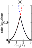
Figure 3: Quench from $\gamma=-50$ to $\gamma=0$ in the system of $N=50$ particles bouncing on a mirror which is located at $x=0$, where $x$ is expressed in the gravitational units. The system is prepared initially in the symmetry broken state $|\psi(t)\rangle=|\psi_{R}(t)\rangle$. Panel (a): $\lambda^{(N)}_{R}$ (dashed red line) and $\lambda^{(N)}_{L}$ (dotted blue line) have been obtained by calculating the projections $|\langle\psi_{L,R}(t)|\tilde{\psi}(t)\rangle|^{2}$ while $\lambda$ (black circles) has been determined from $-N^{-1}\ln[{\cal P}(t)]$. The results indicate that even for relatively small particle number $\lambda(t)$ coincides with ${\rm min}[\lambda^{(N)}_{L}(t),\lambda^{(N)}_{R}(t)]$. Panel (b): left column illustrates evolution of the density of particles right after the quench, i.e. at $t$ equal $t_{0}$, $t_{0}+\frac{\pi}{\omega}$ and $t_{0}+\frac{2\pi}{\omega}$ from top to bottom, respectively. Middle column presents the particle density at similar time moments but around $t=t_{c}$ while the right column corresponds to analogues plots around $t=2t_{c}$. One can see that in the middle column both wavepackets $\phi_{1,2}(x,t)$ are occupied by particles. At moments of time when the wavepackets do not overlap, it is easy to determine their occupations by particles, $|\alpha_{1,2}|^{2}$, and consequently the rates $\lambda^{(N)}_{L,R}=-\ln|\alpha_{1,2}|^{2}$.

III Conclusions

In summary, we have shown that the dynamical quantum phase transitions are not restricted to time independent problems and can also occur in periodically driven systems. In particular, the dynamical quantum phase transitions can be observed in discrete time crystals. The Loschmidt echo is related to the return probability of the system after a quench to the initial periodically evolving Floquet eigenstate. We have shown that the first derivative of the rate function of the Loschmidt echo is discontinuous at $t=t_{c}$. The cusp in the Lochschmidt echo is a signature of passing the critical point between the discrete time crystal regime and the regime where no spontaneous time translation symmetry breaking can be observed. Non-analytical behavior of the corresponding rate function has been proven with the help of the so-called continuum approximation where the Hamiltonian of the many-body system is reduced to the one-body Hamiltonian of a fictitious particle. Dynamical quantum phase transition takes place in the thermodynamic limit which corresponds to the infinite mass of the fictitious particle. The dynamical quantum phase transition described here can be observed in discrete time crystal experiments if the system is prepared in a state which reveals time translation symmetry breaking.

APPENDIX A:
Time evolution after a quench within the continuum approximation

In the main text we consider a model of a discrete time crystal (DTC), whose description, in the periodically evolving basis, reduces to a $N$-body two-mode Hamiltonian

$$\hat{H} = -\frac{J}{2}(\hat{a}_{1}^{\dagger}\hat{a}_{2}+\hat{a}_{2}^{\dagger}\hat{a}_{1})+\frac{U}{2}(\hat{a}_{1}^{\dagger}\hat{a}_{1}^{\dagger}\hat{a}_{1}\hat{a}_{1}+\hat{a}_{2}^{\dagger}\hat{a}_{2}^{\dagger}\hat{a}_{2}\hat{a}_{2})$$ (A.2)

$$+2U_{12}\hat{a}_{1}^{\dagger}\hat{a}_{1}\hat{a}_{2}^{\dagger}\hat{a}_{2},$$

where $\hat{a}_{1,2}$ are standard bosonic operators which annihilate particles in the periodically evolving modes $\phi_{1,2}(x,t)$, $J$ is hopping amplitude while $U$ and $U_{12}$ are interaction strengths between particles in the same and different modes respectively. A relative interaction strength can be quantified by a dimensional parameter $\gamma=N(U-2U_{12})/J$.

In the thermodynamical limit, i.e. where $N\rightarrow\infty$ but $\gamma=$constant, the model has a quantum critial point at $\gamma=-1$ which separates a trivial and a DTC phase. In the DTC phase, i.e. for $\gamma<-1$, low-lying eigenstates of (A.2) are vulnerable to any perturbation and spontaneous breaking of the discrete time translation can be observed Sacha (2015a); Sacha and Zakrzewski (2018).

Here, we describe the time evolution of the system when one starts with the DTC regime and prepares the system either in the symmetric ground state of (A.2) or one of the lowest symmetry broken states. After the quench through the quantum critical point to the trivial phase (i.e. to $\gamma=0$) we observe singularities of the rate of the Loschmidt echo in time, see the main text. The after-quench evolution is described analytically within the so-called continuum approximation Ziń et al. (2008).

III.1 Continuous Hamiltonian

Let us write the Schrödinger equation of the system in the Fock basis

$$\langle n,N-n|\hat{H}|\psi\rangle=E\langle n,N-n|\psi\rangle,$$ (A.3)

where $|\psi\rangle=\sum_{n}\psi_{n}|N-n,n\rangle$, or explicitly

$$\frac{JN}{2}\left(\psi_{n+1}\sqrt{\frac{1+z_{n}}{2}\left(\frac{1-z_{n}}{2}+\frac{1}{N}\right)}\right.+$$ (A.4)

$$\left.\psi_{n-1}\sqrt{\frac{1-z_{n}}{2}\left(\frac{1+z_{n}}{2}+\frac{1}{N}\right)}-\frac{\gamma}{2}\psi_{n}z_{n}^{2}\right)=E\psi_{n}.$$ (A.5)

For $N\gg 1$ we can treat the relative population difference $z_{n}=\frac{(N-n)-n}{N}$ as a continuous variable $z$ with the condition that $|z|\leq 1$, and $\psi(z_{n})=\psi_{n}$ as continuous wavefunction of a fictitious particle. The continuum approximation reduces the many-body Hamiltonian (A.2) to

$$\hat{H}=-\frac{J}{N}\sqrt{1-z^{2}}\frac{\partial^{2}}{\partial{z^{2}}}+V(z),$$ (A.6)

where the effective potential reads

$$V(z)=\frac{JN}{2}\left(-\sqrt{1-z^{2}}+\frac{\gamma}{2}z^{2}\right).$$ (A.7)

For the latter convenience we set $J=1$.

III.2 Ground state manifold

For $\gamma<-1$ the effective potential $V(z)$ has a double well structure and the lowest energy eigenstates of (A.6) can be approximated by

$$\psi_{\pm}(z)=[\psi_{L}(z)\pm\psi_{R}(z)]/\sqrt{2}$$ (A.8)

where $\psi_{L,R}(z)$ are Gaussian states

$$\psi_{L,R}(z)=\frac{1}{(2\pi\sigma^{2})^{1/4}}e^{-\frac{\left(z\pm q\right)^{2}}{4\sigma^{2}}},$$ (A.9)

where $q=\sqrt{1-\gamma^{-2}}$, $\sigma=1/\sqrt{N\Omega}$ and $\Omega=\sqrt{\gamma(1-\gamma^{2})}/(1-q^{2})^{1/4}$. The Gaussian states are the harmonic oscillator ground states obtained by harmonic expansions of $V(z)$ around the two local minima $\pm q$

$$V(z\approx\pm q)\approx N\tilde{\Omega}^{2}(z\mp q)^{2}/4+\mbox{constant},$$ (A.10)

where $\tilde{\Omega}=\Omega(1-q^{2})^{1/4}$ and by substituting $\sqrt{1-q^{2}}$ for $\sqrt{1-z^{2}}$ in (A.6). For fixed $\gamma$, the larger $N$, the more localized Gaussian states because the total number of particles $N$ is proportional to the mass of the fictitious particle described by the Hamiltonian (A.6).

III.3 After-quench evolution

Let us assume that for large but finite $N$ the system is initially prepared in the symmetric ground state $\psi(z,0)=\psi_{+}(z)$ (A.8). At $t=t_{0}=0$ we set $\gamma=0$ and describe the time evolution of the system by means of the continuous Hamiltonian (A.6) where the term $\sqrt{1-z^{2}}$ is neglected.

$$\tilde{\psi}(z,t) = \int\mbox{d}z^{\prime}K(z,t;z^{\prime})\psi_{+}(z),$$ (A.11)

$$K(z,t;z^{\prime}) = \sqrt{\frac{a(t)}{\pi i}}e^{ia(t)\left[\left(z^{2}+z^{\prime 2}\right)\cos(t)-2zz^{\prime}\right]},$$ (A.12)

where $a(t)=N/\left(4\sin(t)\right)$. Explicitly we obtain

$$\tilde{\psi}(z,t) = [\tilde{\psi}_{L}(z,t)+\tilde{\psi}_{R}(z,t)]/\sqrt{2}\,,$$ (A.14)

$$\tilde{\psi}_{L,R}(z,t) = A(t)e^{-B(t)z^{2}\pm iC(t)z+D(t)},$$ (A.15)

where

$$A(t) = \sqrt{\frac{-ia(t)}{b(t)\sqrt{2\pi\sigma^{2}}}},$$ (A.16)

$$B(t) = -a(t)\cos(t)+\frac{a(t)^{2}}{b(t)},$$ (A.17)

$$C(t) = \frac{|q|a(t)}{2\sigma^{2}b(t)},$$ (A.18)

$$D(t) = \frac{q^{2}}{4\sigma^{2}}\left(-1+\frac{1}{4\sigma^{2}b(t)}\right),$$ (A.19)

$$b(t) = \frac{1}{4\sigma^{2}}-ia(t)\cos(t).$$ (A.20)

III.4 Loschmidt echo and rate function

In this part we give explicit formulas, within the continuum approximation, for the Loschmidt echo and the rate function Heyl (2017) when initially the system is prepared in the symmetric ground state (A.8). The initial state is written in the periodically evolving basis and corresponds to the Floquet state that fulfils the discrete time translation symmetry of the original time-dependent Hamiltonian.

The probability of the return of the evolving $N$-body state $|\tilde{\psi}_{+}(t)\rangle=\sum_{n}\tilde{\psi}(z_{n},t>t_{0})|N-n,n\rangle$ to the time-periodic Floquet symmetric eigenstate $|\psi_{+}(t)\rangle$, is given by the Loschmidt echo $|{\cal G}(t>t_{0})|^{2}$, where

$${\cal G}(t>t_{0})=\langle\psi_{+}(t)|\tilde{\psi}_{+}(t)\rangle$$ (A.21)

is called the Loschmidt amplitude. Within the continuum approximation (A.21) is equivalent to

$${\cal G}(t)=\int\psi^{*}_{+}(z)\tilde{\psi}(z,t).$$ (A.22)

The Loschmidt amplitude (A.22) can be written in terms of the symmetry broken states (A.8) and (A.14), namely

$${\cal G}(t)=\int\psi^{*}_{L}(z)\tilde{\psi}_{L}(z,t)+\int\psi^{*}_{R}(z)\tilde{\psi}_{L}(z,t)=$$

$$=\int\psi^{*}_{R}(z)\tilde{\psi}_{R}(z,t)+\int\psi^{*}_{L}(z)\tilde{\psi}_{R}(z,t)=$$

$$\equiv{\cal G}_{R}(t)+{\cal G}_{L}(t),$$ (A.23)

where, after a conscientious calculation we obtain:

$${\cal G}_{R}(t) = \sqrt{\frac{-ia(t)}{2\sigma^{2}b(t)c(t)}}e^{-\frac{N}{2}\left(\lambda_{R}(t)+i\mu_{R}(t)\right)},$$ (A.24)

$${\cal G}_{L}(t) = \sqrt{\frac{-ia(t)}{2\sigma^{2}b(t)c(t)}}e^{-\frac{N}{2}\left(\lambda_{L}(t)+i\mu_{L}(t)\right)},$$ (A.25)

where

$$c(t) = -ia(t)\cos(t)+\frac{a(t)^{2}}{b(t)}+\frac{1}{4\sigma^{2}},$$ (A.26)

and

$$\lambda_{R}(t) = \frac{q^{2}\tilde{\Omega}\tan^{2}(\frac{t}{2})}{\tilde{\Omega}^{2}+\tan^{2}(\frac{t}{2})},$$ (A.27)

$$\mu_{R}(t) = \frac{q^{2}\tilde{\Omega}^{2}\tan(\frac{t}{2})}{\tilde{\Omega}^{2}+\tan^{2}(\frac{t}{2})},$$ (A.28)

$$\lambda_{L}(t) = \frac{q^{2}\tilde{\Omega}\cot^{2}(\frac{t}{2})}{\tilde{\Omega}^{2}+\cot^{2}(\frac{t}{2})},$$ (A.29)

$$\mu_{L}(t) = \frac{-\,q^{2}\tilde{\Omega}^{2}\cot(\frac{t}{2})}{\tilde{\Omega}^{2}+\cot^{2}(\frac{t}{2})}.$$ (A.30)

The Loschmidt echo for non-critical states scales exponentially with the total number of particles $N$ Heyl (2017). Therefore, it is convenient to consider an intensive quantity, i.e. the rate of the Loschmidt echo

$$\lambda_{+}(t)=\lim\limits_{N\rightarrow\infty}\lambda_{+}^{(N)}(t),\quad\lambda_{+}^{(N)}=-N^{-1}\ln|{\cal G}(t)|^{2}.$$ (A.31)

A straightforward calculations shows that in the thermodynamical limit

$$\lambda_{+}(t)=\min\left(\lambda_{R}(t),\lambda_{L}(t)\right).$$ (A.32)

The rate function (A.32) has a non-analytic cusp for $t=t_{c}=\pi/2$ when $\lambda_{R}=\lambda_{L}$. This cusp results in discontinuity of the first derivate of the rate function

$$\lim\limits_{t\rightarrow t_{c}^{\pm}}\frac{d\lambda_{+}(t)}{dt}=\lim\limits_{t\rightarrow t_{c}^{\pm}}\lim\limits_{N\rightarrow\infty}\frac{d\lambda_{+}^{(N)}(t)}{dt}=\mp\frac{2q^{2}\Omega^{3}}{(1+\Omega^{2})^{2}}.$$ (A.33)

It should be stressed that the order of the limits is important. Indeed, $\lim\limits_{t\rightarrow t_{c}}\lambda_{+}(t)$ is defined but

$$\lim\limits_{N\rightarrow\infty}\lambda_{+}^{(N)}(t_{c})=\frac{q^{2}\Omega}{1+\Omega^{2}}-\lim_{N\rightarrow\infty}\frac{1}{N}\ln\left[\cos^{2}\left(\frac{Nq^{2}\Omega^{2}}{2(1+\Omega^{2})}\right)\right],$$ (A.34)

is not because whenever the cosine in (A.34) is close to zero, the logarithm diverges which corresponds to accidental values of $N$ for which the Loschmidt echo vanishes.

APPENDIX B:
Calculation of entanglement entropy

In this section we present the calculation of the non-analytical jump of the entanglement entropy $S(t)$ at the critical point $t=t_{c}$ when the system is initially prepared in the symmetric Floquet state $\psi_{+}(z)$ (A.8).

The von Neumann entropy of the reduced density matrix of the system after the quench is defined as

$$S(t>t_{0})=-\mbox{tr}\left(\rho_{1}\ln\rho_{1}\right),$$ (B.1)

where

$$\rho_{1}=\sum_{n_{2}}\langle n_{2}|\tilde{\psi}_{+}(t)\rangle\langle\tilde{\psi}_{+}(t)|n_{2}\rangle.$$ (B.2)

After decomposing the Floquet state in the Fock basis $|\tilde{\psi}_{+}(t)\rangle=\sum_{n}\tilde{\psi}(z_{n},t)|n,N-n\rangle$ a straightforward calculation leads to

$$S(t)=-\sum_{n}|\tilde{\psi}(z_{n},t)|^{2}\ln|\tilde{\psi}(z_{n},t)|^{2}.$$ (B.3)

Let us first consider $S(t)$ away from the critical time. Applying the continuum approximation we obtain

$$S(t\neq t_{c})=-\int|\tilde{\psi}|^{2}\ln|\tilde{\psi}|^{2}\approx\ln 2\,+$$

$$-\frac{1}{2}\left(\int|\tilde{\psi}_{L}|^{2}\ln|\tilde{\psi}_{L}|^{2}+\int|\tilde{\psi}_{R}|^{2}\ln|\tilde{\psi}_{R}|^{2}\right),$$ (B.4)

where we have used the fact that away from the critical time $|\tilde{\psi}|^{2}\approx[|\tilde{\psi}_{L}|^{2}+|\tilde{\psi}_{R}|^{2}]/2$ for $N\gg 1$. For sufficiently large $N$, (B.4) holds for any $t$ arbitrary close to $t_{c}$. In particular

$$\lim_{t\rightarrow t_{c}^{\pm}}S(t\neq t_{c})\approx\ln 2-\int|\tilde{\psi}_{0}|^{2}\ln|\tilde{\psi}_{0}|^{2},$$ (B.5)

where , from (A.14)-(A.15), we have

$$|\tilde{\psi}_{0}|^{2}=\lim_{t\rightarrow t_{c}}|\tilde{\psi}_{L/R}|^{2}=\sqrt{\frac{2}{\pi N\Omega}}\;e^{-Nz^{2}/(2\Omega)}.$$ (B.6)

On the other hand, exactly at $t=t_{c}$ one gets

$$S(t_{c})=-\int\left|\frac{\tilde{\psi}_{0}e^{i\beta z}+\tilde{\psi}_{0}e^{-i\beta z}}{\sqrt{2}}\right|^{2}\ln\left|\frac{\tilde{\psi}_{0}e^{i\beta z}+\tilde{\psi}_{0}e^{-i\beta z}}{\sqrt{2}}\right|^{2}$$

$$\approx-\int|\tilde{\psi}_{0}|^{2}\ln|\tilde{\psi}_{0}|^{2}-\int|\tilde{\psi}_{0}|^{2}\cos(2\beta z)\,+$$

$$-2\int|\tilde{\psi}_{0}|^{2}\cos^{2}(\beta z)\ln\left(1+\cos(2\beta z)\right),$$ (B.7)

where $\beta=Nq/2$. Note that because of the presence of $\cos^{2}(\beta z)$ there are no singular points under the integral in the second term. Subtracting (B.7) from (B.4) we obtain

$$\delta S(t_{c}) \equiv \lim_{t\rightarrow t_{c}^{\pm}}S(t\neq t_{c})-S(t_{c})$$ (B.8)

$$\approx \ln 2+2\int|\tilde{\psi}_{0}|^{2}\cos(2\beta z)$$ (B.10)

$$+\sum_{n=2}^{\infty}\int|\tilde{\psi}_{0}|^{2}\frac{(-1)^{n}}{n(n-1)}\cos^{n}(2\beta z),$$

where a series expansion of the logarithm was used. Highly oscillatory terms in (LABEL:appB:entropy_diff) can be dropped if $N\gg 1$. Note that

$$\cos^{n}(2\beta z)=\left(\frac{e^{2i\beta z}+e^{-2i\beta z}}{2}\right)^{n}=\sum_{k=0}^{n}\left(\begin{matrix}n\\ k\end{matrix}\right)\frac{e^{2i\beta z(n-2k)}}{2^{n}}$$ (B.12)

and that the only non-oscilatory term in the sum (B.12) corresponds to $k=n/2$. Using this result in (LABEL:appB:entropy_diff) we finally get

$$\delta S(t_{c})\approx\ln 2+\sum_{m=1}^{\infty}\left(\begin{matrix}2m\\ m\end{matrix}\right)\frac{1}{2m(2m-1)4^{m}}=1.$$ (B.13)

References

- Sachdev (2011) S. Sachdev, Quantum Phase Transitions (Cambridge University Press, Cambridge, 2011).
- Sachdev and Keimer (2011) S. Sachdev and B. Keimer, Physics Today 64, 29 (2011), URL http://physicstoday.scitation.org/doi/10.1063/1.3554314.
- Eckstein et al. (2009) M. Eckstein, M. Kollar, and P. Werner, Phys. Rev. Lett. 103, 056403 (2009), URL https://link.aps.org/doi/10.1103/PhysRevLett.103.056403.
- Garrahan and Lesanovsky (2010) J. P. Garrahan and I. Lesanovsky, Phys. Rev. Lett. 104, 160601 (2010), URL https://link.aps.org/doi/10.1103/PhysRevLett.104.160601.
- Diehl et al. (2010) S. Diehl, A. Tomadin, A. Micheli, R. Fazio, and P. Zoller, Phys. Rev. Lett. 105, 015702 (2010), URL https://link.aps.org/doi/10.1103/PhysRevLett.105.015702.
- Schiró and Fabrizio (2010) M. Schiró and M. Fabrizio, Phys. Rev. Lett. 105, 076401 (2010), URL https://link.aps.org/doi/10.1103/PhysRevLett.105.076401.
- Sciolla and Biroli (2010) B. Sciolla and G. Biroli, Phys. Rev. Lett. 105, 220401 (2010), URL https://link.aps.org/doi/10.1103/PhysRevLett.105.220401.
- Sciolla and Biroli (2011) B. Sciolla and G. Biroli, Journal of Statistical Mechanics: Theory and Experiment 2011, P11003 (2011), URL http://stacks.iop.org/1742-5468/2011/i=11/a=P11003.
- Ates et al. (2012) C. Ates, B. Olmos, J. P. Garrahan, and I. Lesanovsky, Phys. Rev. A 85, 043620 (2012), URL https://link.aps.org/doi/10.1103/PhysRevA.85.043620.
- Sciolla and Biroli (2013) B. Sciolla and G. Biroli, Phys. Rev. B 88, 201110 (2013), URL https://link.aps.org/doi/10.1103/PhysRevB.88.201110.
- Vosk and Altman (2014) R. Vosk and E. Altman, Phys. Rev. Lett. 112, 217204 (2014), URL https://link.aps.org/doi/10.1103/PhysRevLett.112.217204.
- Žunkovič et al. (2016) B. Žunkovič, A. Silva, and M. Fabrizio, Phil. Trans. R. Soc. A 374, 20150160 (2016), URL http://rsta.royalsocietypublishing.org/content/374/2069/20150160.
- Maraga et al. (2016) A. Maraga, P. Smacchia, and A. Silva, Phys. Rev. B 94, 245122 (2016), URL https://link.aps.org/doi/10.1103/PhysRevB.94.245122.
- Heyl et al. (2013) M. Heyl, A. Polkovnikov, and S. Kehrein, Phys. Rev. Lett. 110, 135704 (2013), URL https://link.aps.org/doi/10.1103/PhysRevLett.110.135704.
- Heyl (2015) M. Heyl, Phys. Rev. Lett. 115, 140602 (2015), URL https://link.aps.org/doi/10.1103/PhysRevLett.115.140602.
- Budich and Heyl (2016) J. C. Budich and M. Heyl, Phys. Rev. B 93, 085416 (2016), URL https://link.aps.org/doi/10.1103/PhysRevB.93.085416.
- Sharma et al. (2016) S. Sharma, U. Divakaran, A. Polkovnikov, and A. Dutta, Phys. Rev. B 93, 144306 (2016), URL https://link.aps.org/doi/10.1103/PhysRevB.93.144306.
- Bhattacharya and Dutta (2017) U. Bhattacharya and A. Dutta, Phys. Rev. B 96, 014302 (2017), URL https://link.aps.org/doi/10.1103/PhysRevB.96.014302.
- Bhattacharya et al. (2017) U. Bhattacharya, S. Bandyopadhyay, and A. Dutta, Phys. Rev. B 96, 180303 (2017), URL https://link.aps.org/doi/10.1103/PhysRevB.96.180303.
- Karrasch and Schuricht (2017) C. Karrasch and D. Schuricht, Phys. Rev. B 95, 075143 (2017), URL https://link.aps.org/doi/10.1103/PhysRevB.95.075143.
- Heyl and Budich (2017) M. Heyl and J. C. Budich, Phys. Rev. B 96, 180304 (2017), URL https://link.aps.org/doi/10.1103/PhysRevB.96.180304.
- Halimeh and Zauner-Stauber (2017) J. C. Halimeh and V. Zauner-Stauber, Phys. Rev. B 96, 134427 (2017), URL https://link.aps.org/doi/10.1103/PhysRevB.96.134427.
- Zauner-Stauber and Halimeh (2017) V. Zauner-Stauber and J. C. Halimeh, Phys. Rev. E 96, 062118 (2017), URL https://link.aps.org/doi/10.1103/PhysRevE.96.062118.
- Homrighausen et al. (2017) I. Homrighausen, N. O. Abeling, V. Zauner-Stauber, and J. C. Halimeh, Phys. Rev. B 96, 104436 (2017), URL https://link.aps.org/doi/10.1103/PhysRevB.96.104436.
- Lang et al. (2017) J. Lang, B. Frank, and J. C. Halimeh, ArXiv e-prints (2017), eprint 1712.02175.
- Zunkovic et al. (2016) B. Zunkovic, M. Heyl, M. Knap, and A. Silva, ArXiv e-prints (2016), eprint 1609.08482.
- Fläschner et al. (2016) N. Fläschner, D. Vogel, M. Tarnowski, B. S. Rem, D.-S. Lühmann, M. Heyl, J. C. Budich, L. Mathey, K. Sengstock, and C. Weitenberg, ArXiv e-prints (2016), eprint 1608.05616.
- Jurcevic et al. (2017) P. Jurcevic, H. Shen, P. Hauke, C. Maier, T. Brydges, C. Hempel, B. P. Lanyon, M. Heyl, R. Blatt, and C. F. Roos, Phys. Rev. Lett. 119, 080501 (2017), URL https://link.aps.org/doi/10.1103/PhysRevLett.119.080501.
- Heyl (2017) M. Heyl, ArXiv e-prints (2017), eprint 1709.07461.
- Wilczek (2012) F. Wilczek, Phys. Rev. Lett. 109, 160401 (2012), URL http://link.aps.org/doi/10.1103/PhysRevLett.109.160401.
- Bruno (2013) P. Bruno, Phys. Rev. Lett. 111, 070402 (2013), URL http://link.aps.org/doi/10.1103/PhysRevLett.111.070402.
- Watanabe and Oshikawa (2015) H. Watanabe and M. Oshikawa, Phys. Rev. Lett. 114, 251603 (2015), URL http://link.aps.org/doi/10.1103/PhysRevLett.114.251603.
- Syrwid et al. (2017) A. Syrwid, J. Zakrzewski, and K. Sacha, ArXiv e-prints (2017), eprint 1702.05006.
- Iemini et al. (2017) F. Iemini, A. Russomanno, J. Keeling, M. Schirò, M. Dalmonte, and R. Fazio, ArXiv e-prints (2017), eprint 1708.05014.
- Huang et al. (2017a) Y. Huang, T. Li, and Z.-q. Yin, ArXiv e-prints (2017a), eprint 1709.07657.
- Prokof’ev and Svistunov (2017) N. V. Prokof’ev and B. V. Svistunov, ArXiv e-prints (2017), eprint 1710.00721.
- Sacha (2015a) K. Sacha, Phys. Rev. A 91, 033617 (2015a), URL http://link.aps.org/doi/10.1103/PhysRevA.91.033617.
- Khemani et al. (2016) V. Khemani, A. Lazarides, R. Moessner, and S. L. Sondhi, Phys. Rev. Lett. 116, 250401 (2016), URL http://link.aps.org/doi/10.1103/PhysRevLett.116.250401.
- Else et al. (2016) D. V. Else, B. Bauer, and C. Nayak, Phys. Rev. Lett. 117, 090402 (2016), URL http://link.aps.org/doi/10.1103/PhysRevLett.117.090402.
- Yao et al. (2017) N. Y. Yao, A. C. Potter, I.-D. Potirniche, and A. Vishwanath, Phys. Rev. Lett. 118, 030401 (2017), URL http://link.aps.org/doi/10.1103/PhysRevLett.118.030401.
- Lazarides and Moessner (2017) A. Lazarides and R. Moessner, Phys. Rev. B 95, 195135 (2017), URL https://link.aps.org/doi/10.1103/PhysRevB.95.195135.
- Russomanno et al. (2017) A. Russomanno, F. Iemini, M. Dalmonte, and R. Fazio, Phys. Rev. B 95, 214307 (2017), URL https://link.aps.org/doi/10.1103/PhysRevB.95.214307.
- Zeng and Sheng (2017) T.-S. Zeng and D. N. Sheng, Phys. Rev. B 96, 094202 (2017), URL https://link.aps.org/doi/10.1103/PhysRevB.96.094202.
- Nakatsugawa et al. (2017) K. Nakatsugawa, T. Fujii, and S. Tanda, Phys. Rev. B 96, 094308 (2017), URL https://link.aps.org/doi/10.1103/PhysRevB.96.094308.
- Ho et al. (2017) W. W. Ho, S. Choi, M. D. Lukin, and D. A. Abanin, Phys. Rev. Lett. 119, 010602 (2017), URL https://link.aps.org/doi/10.1103/PhysRevLett.119.010602.
- Huang et al. (2017b) B. Huang, Y.-H. Wu, and W. V. Liu, ArXiv e-prints (2017b), eprint 1703.04663.
- Gong et al. (2017) Z. Gong, R. Hamazaki, and M. Ueda, ArXiv e-prints (2017), eprint 1708.01472.
- Wang et al. (2017) R. R. W. Wang, B. Xing, G. G. Carlo, and D. Poletti, ArXiv e-prints (2017), eprint 1708.09070.
- Zhang et al. (2017) J. Zhang, P. W. Hess, A. Kyprianidis, P. Becker, A. Lee, J. Smith, G. Pagano, I.-D. Potirniche, A. C. Potter, A. Vishwanath, et al., Nature 543, 217 (2017), ISSN 0028-0836, letter, URL http://dx.doi.org/10.1038/nature21413.
- Choi et al. (2017) S. Choi, J. Choi, R. Landig, G. Kucsko, H. Zhou, J. Isoya, F. Jelezko, S. Onoda, H. Sumiya, V. Khemani, et al., Nature 543, 221 (2017), ISSN 0028-0836, letter, URL http://dx.doi.org/10.1038/nature21426.
- Nayak (2017) C. Nayak, Nature 543, 185 (2017), ISSN 0028-0836, news & Views, URL http://dx.doi.org/10.1038/543185a.
- Kim et al. (2006) K. Kim, M.-S. Heo, K.-H. Lee, K. Jang, H.-R. Noh, D. Kim, and W. Jhe, Phys. Rev. Lett. 96, 150601 (2006), URL https://link.aps.org/doi/10.1103/PhysRevLett.96.150601.
- Heo et al. (2010) M.-S. Heo, Y. Kim, K. Kim, G. Moon, J. Lee, H.-R. Noh, M. I. Dykman, and W. Jhe, Phys. Rev. E 82, 031134 (2010), URL https://link.aps.org/doi/10.1103/PhysRevE.82.031134.
- Guo et al. (2013) L. Guo, M. Marthaler, and G. Schön, Phys. Rev. Lett. 111, 205303 (2013), URL https://link.aps.org/doi/10.1103/PhysRevLett.111.205303.
- Sacha (2015b) K. Sacha, Sci. Rep. 5, 10787 (2015b), URL https://www.nature.com/articles/srep10787.
- Sacha and Delande (2016) K. Sacha and D. Delande, Phys. Rev. A 94, 023633 (2016), URL http://link.aps.org/doi/10.1103/PhysRevA.94.023633.
- Guo and Marthaler (2016) L. Guo and M. Marthaler, New Journal of Physics 18, 023006 (2016), URL http://stacks.iop.org/1367-2630/18/i=2/a=023006.
- Guo et al. (2016) L. Guo, M. Liu, and M. Marthaler, Phys. Rev. A 93, 053616 (2016), URL https://link.aps.org/doi/10.1103/PhysRevA.93.053616.
- Giergiel and Sacha (2017) K. Giergiel and K. Sacha, Phys. Rev. A 95, 063402 (2017), URL https://link.aps.org/doi/10.1103/PhysRevA.95.063402.
- Mierzejewski et al. (2017) M. Mierzejewski, K. Giergiel, and K. Sacha, Phys. Rev. B 96, 140201 (2017), URL https://link.aps.org/doi/10.1103/PhysRevB.96.140201.
- Delande et al. (2017) D. Delande, L. Morales-Molina, and K. Sacha, Phys. Rev. Lett. 119, 230404 (2017), URL https://link.aps.org/doi/10.1103/PhysRevLett.119.230404.
- Flicker (2017) F. Flicker, ArXiv e-prints (2017), eprint 1707.09371.
- Liang et al. (2017) P. Liang, M. Marthaler, and L. Guo, ArXiv e-prints (2017), eprint 1710.09716.
- Giergiel et al. (2017) K. Giergiel, A. Miroszewski, and K. Sacha, ArXiv e-prints (2017), eprint 1710.10087.
- Sacha and Zakrzewski (2018) K. Sacha and J. Zakrzewski, Rep. Prog. Phys. 81, 016401 (2018), URL https://doi.org/10.1088/1361-6633/aa8b38.
- Steane et al. (1995) A. Steane, P. Szriftgiser, P. Desbiolles, and J. Dalibard, Phys. Rev. Lett. 74, 4972 (1995), URL http://link.aps.org/doi/10.1103/PhysRevLett.74.4972.
- Lau et al. (1999) D. C. Lau, A. I. Sidorov, G. I. Opat, R. J. McLean, W. J. Rowlands, and P. Hannaford, Eur. Phys. J. D 5, 193 (1999), URL https://doi.org/10.1007/s100530050244.
- Bongs et al. (1999) K. Bongs, S. Burger, G. Birkl, K. Sengstock, W. Ertmer, K. Rza̧żewski, A. Sanpera, and M. Lewenstein, Phys. Rev. Lett. 83, 3577 (1999), URL https://link.aps.org/doi/10.1103/PhysRevLett.83.3577.
- Buchleitner et al. (2002) A. Buchleitner, D. Delande, and J. Zakrzewski, Physics reports 368, 409 (2002), URL http://www.sciencedirect.com/science/article/pii/S0370157302002703.
- Raghavan et al. (1999) S. Raghavan, A. Smerzi, S. Fantoni, and S. R. Shenoy, Phys. Rev. A 59, 620 (1999), URL https://link.aps.org/doi/10.1103/PhysRevA.59.620.
- Ziń et al. (2008) P. Ziń, J. Chwedeńczuk, B. Oleś, K. Sacha, and M. Trippenbach, EPL (Europhysics Letters) 83, 64007 (2008), URL http://stacks.iop.org/0295-5075/83/i=6/a=64007.
- Oleś et al. (2010) B. Oleś, P. Ziń, J. Chwedeńczuk, K. Sacha, and M. Trippenbach, Laser Physics 20, 671 (2010), URL https://doi.org/10.1134/S1054660X10050130.
- Milburn et al. (1997) G. J. Milburn, J. Corney, E. M. Wright, and D. F. Walls, Phys. Rev. A 55, 4318 (1997), URL https://link.aps.org/doi/10.1103/PhysRevA.55.4318.
- Heyl (2017) M. Heyl, Phys. Rev. B 95, 060504 (2017), URL https://link.aps.org/doi/10.1103/PhysRevB.95.060504.