What can we learn on supernova neutrino spectra
with water Cherenkov detectors?

Abstract

We investigate the precision with which the supernova neutrino spectra can be reconstructed in water Cherenkov detectors, in particular the large scale Hyper-Kamiokande and Super-Kamiokande. To this aim, we consider quasi-thermal neutrino spectra modified by the Mikheev-Smirnov-Wolfenstein effect for the case of normal ordering. We perform three 9 degrees of freedom likelihood analyses including first inverse-beta decay only, then the combination of inverse beta decay and elastic scattering on electrons and finally a third analysis that also includes neutral scattering neutrino-oxygen events. A tenth parameter is added in the analyses to account for the theoretical uncertainty on the neutral current neutrino-oxygen cross section. By assuming a 100% efficiency in Hyper-Kamiokande, we show that one can reconstruct the electron antineutrino average energy and pinching parameter with an accuracy of $\sim 2\%$ and $\sim 7\%$ percent respectively, while the antineutrino integrated luminosity can be pinned down at $\sim 3\%$ percent level. As for the muon and tau neutrinos, the average energy and the integrated luminosity can be measured with $\sim 7\%$ precision. These results represent a significant improvement with respect Super-Kamiokande, particularly for the pinching parameter defining the electron antineutrino spectra. As for electron neutrinos, the determination of the emission parameters requires the addition of supplementary detection channels.

1 Introduction

Unravelling the mechanisms for iron core-collapse supernovae is a longstanding open question in astrophysics. The main ideas on the explosion mechanism were already outlined in the sixties when it was first accepted that a massive star would undergo a core collapse at the end of its life. According to Colgate and Johnson’s prompt-shock model, core bounce would create a shock that would propagate and expel the star’s mantle [1]. Colgate and White suggested that the gravitational binding energy of the newly formed proto-neutron star would be released mostly as neutrinos, in a short burst lasting few seconds. A fraction of the order of a few percent of this energy could be deposited behind the shock and drive the explosion [2]. This turned into the delayed-accretion shock paradigm, proposed in the work of Wilson [3] and discussed since then, beginning with the works of Nadyozhin [4] and of Bethe and Wilson [5].

Core-collapse supernova neutrinos have been first observed during SN 1987A in the Large Magellanic Cloud through inverse beta decay in the Kamiokande [6], IMB [7] and Baksan detectors [8]. The LSD/Mont Blanc data occurring a few hours before the others [9] have been debated (see e.g. [10]). The time dependence of twenty-nine neutrino events has supported the delayed-accretion shock model, in contrast to the prompt one, as shown by the in-depth analysis of Loredo and Lamb [11] and as confirmed by the completely independent analysis of ref. [12]. Based on the hypothesis of energy equipartition among the neutrino flavors, the gravitational binding energy of the newly formed neutron star is found to be approximatively $3\text{\times}{10}^{53}\text{\,}\mathrm{erg}$, in agreement with predictions. Moreover, the SN 1987A neutrino spectra do not contradict the hypothesis of quasi-thermal distribution, with emission temperatures of about $4\text{\,}\mathrm{MeV}$ (see [13] for a systematic investigation).

State-of-the-art supernova simulations are multi-dimensional, include realistic neutrino transport, nuclear networks, convection and hydrodynamic instabilities such as the Standing-Accretion-Shock-Instability (SASI) [14]. The detection of the supernova neutrino time signal from a future explosion will represent a direct test of the SASI-aided delayed-accretion shock mechanism (see e.g. [15]). This is thought to explain the majority of supernova explosions, except the most violent ones that might be magneto-hydrodynamically driven [16]. Successful explosions have been obtained in two-dimensions for a set of progenitors. Three-dimensional simulations appear to be at the verge of succeed (see e.g. [16, 17]).

The occurrence of a supernova explosion in the Milky Way will trigger a network of detectors, based on water (or ice) Cherenkov, scintillators and liquid argon detectors, providing the collection of several thousands up to one million events for a prototypical event located at $5\div$10\text{\,}\mathrm{kpc}$$ from the Earth. The precise knowledge of cross sections associated with inverse beta decay and neutrino-electron scattering will allow measurements, free from the systematic errors that still affect neutrino-nucleus cross sections in the several tens of MeV energy range. Neutrino interaction cross sections on nuclei like oxygen, argon, iron and lead at the relevant supernova energies have significant theoretical uncertainties. Measurements are being planned at the SNS facility by the COHERENT Collaboration [18]. These will bring important information on the reaction cross sections and hopefully also on the quenching of the axial-vector coupling constant, that is essential for neutrinoless double beta decay.

According to supernova simulations, the neutrino spectra in the decoupling region are described by quasi-thermal distributions. Three parameters for both electron and non-electron type neutrinos are necessary to describe the spectra, namely the normalization, the average energy and the width. The latter parameter describes the deviation from a perfect thermal distribution, and it is commonly called the “pinching” parameter. This amounts to a set of 9 free parameters. The situation gets more complex when neutrinos enter the free-streaming regime, since the occurrence of flavor conversion phenomena due to neutrino self-interactions, coupling to matter, shock wave effects or turbulence might produce spectral swapping(s). In particular, neutrino self-interactions make neutrino propagation in dense environments a non-linear many-body problem. It still needs to be determined under which conditions neutrino-neutrino interactions produce spectral modifications, and how sizable they are [19]. In the simplest cases the neutrino spectra could be completely degenerate at the neutrino sphere, or neutrino self-interactions could produce flavor equilibration.

The reconstruction of the neutrino spectra and the determination of the total gravitational binding energy of the newly formed neutron star has already been investigated in several works, such as refs. [21, 20, 22]. Of course, the answer to these issues depends on the constraints imposed to the flux parameters in the likelihood analysis. Ref. [21] has studied in great detail the electron antineutrino signal associated with inverse beta decay in water Cherenkov detectors. A six degrees of freedom likelihood analysis of the supernova signal has been performed considering not only the total and the average energies of each neutrino species, but also the pinching parameters. As an outcome, a continuous degeneracy in the reconstructed parameters has been shown to exist, which appears to preclude a precise determination of the supernova neutrino fluxes. Ref. [23] shows that the explosion energy can be determined up to $13\%$ precision at $1\sigma$ confidence level in JUNO detector, assuming however that the pinching is fully known. In ref. [24] we have shown that the combined analysis of events associated with inverse beta decay and electron scattering in water Cherenkov detectors allows to determine the gravitational binding energy of the neutron star with a precision of $11\%$ in a detector like Super-Kamiokande, if a galactic supernova explodes. The addition of neutral current neutrino-oxygen scattering does not change the conclusion because of limited statistics. Finally we have shown that a precise measurement of the gravitational binding energy of the newly formed neutron star allows to determine the star compactness within $10\%$ [24].

In this manuscript, we explore how precisely (all) the supernova emission parameters can be reconstructed using data from water Cherenkov detectors. Differently from ref. [24] we consider Hyper-Kamiokande, that will very likely be built and that one can regard as the ultimate water Cherenkov detector. The outcomes of this analysis are compared with those allowed by Super-Kamiokande, that represents the best that supernova neutrino science can achieve nowadays by means of water Cherenkov detectors. The data set used for the analysis of Super-Kamiokande is the same as the one in ref. [24] with the difference that here we analyze all features of the neutrino spectra. We employ the well-motivated quasi-thermal neutrino spectra assuming that flavor conversion is governed by the Mikheev-Smirnov-Wolfenstein effect [25, 26]. We perform a likelihood analysis with 10 degrees of freedom (9 for the flux parameters +1 for the $\nu$-oxygen cross section uncertainty), leaving in particular the parameters of the electron, muon and tau neutrino fluxes unconstrained. The neutrino mass ordering is not yet known. We fix it to normal, as template case, having in mind that combined analysis of oscillation data show a slight preference for it, although statistical significance is still low [27]. In the present analysis we combine events from inverse beta decay, neutrino-electron elastic scattering and neutral current interactions on oxygen nuclei. The attitude of our investigation is rather conservative, since, in particular, we do not assume any definite energy partition among the neutrino flavors a priori, as most commonly done in previous studies. Our choice is motivated by the fact that the current supernova simulations, albeit not yet definitive, do not support the occurrence of an exact equipartition, neither during the accretion nor during the cooling phases of emission. Nonetheless, we perform also another analysis, where the ansatz on energy equipartition is implemented, to allow a comparison with results available in the literature.

The paper is structured as follows. Section 2 presents the methods employed for the likelihood analysis of the events. The inputs of our calculations are described including the neutrino fluences and the cross sections, and we compare our outcomes with those of ref. [21] when only inverse-beta decay is considered and a 6 degrees of freedom likelihood analysis performed. Section 3 presents the numerical results from the full 10-dimensional likelihood analysis, and section 4 presents our conclusions.

2 Description of the statistical analysis

2.1 Detector properties

In our statistical analysis of a core-collapse supernova explosion, we consider neutrino events as can be seen by water Cherenkov detectors, namely Super-Kamiokande and Hyper-Kamiokande. The former is up to now the largest Cherenkov detector in operation, with a total (fiducial) mass of 50 (22.5) kton of water [28], while the latter should be built in the future and will have a total (fiducial) mass of 516 (374) kton [29]. In this study, as active mass for the two detectors, we consider $22.5\text{\,}\mathrm{kton}$ and $374\text{\,}\mathrm{kton}$ respectively.

Neutrinos in water can be detected thanks to several reactions — see e.g. [30]. The most important one for our purposes, that will be included in the analysis, are the following three:

1. inverse beta decay (IBD): $\mathrm{p}+\overline{\nu}_{\mathrm{e}}\rightarrow\mathrm{n}+\mathrm{e}^{+}$;

2. elastic scattering on electrons (ES): $\nu+\mathrm{e}^{-}\rightarrow\nu+\mathrm{e}^{-}$;

3. neutral current scattering on oxygen (OS): $\nu+\text{\textsuperscript{16}O}\rightarrow\nu+\text{\textsuperscript{16}O}^{*}\rightarrow\nu+\gamma+\text{X}$.

The IBD process provides the highest number of events. The positron emission is, with good approximation, isotropic [31] while the ES events spread out in a cone of about $20^{\circ}$ [32] that points towards the neutrino direction. This is crucial for the ES tagging, because the directional discrimination reduces the IBD background to the portion of the solid angle in which it overlaps to the ES signal (3%). Additional rejections can be performed applying an energy cut — 20% on events with energy lower than 30 MeV [33] — and neutron tagging. In this case, the rejection power is 20% for clear water [33] and reaches 90% with gadolinium-loading [34, 35].

In this study we assume a 100% tagging efficiency on ES (and IBD) events above the detection threshold of $5\text{\,}\mathrm{MeV}$, supposed to be the same for Super-Kamiokande [36, 37] and Hyper-Kamiokande [29]. Concerning the OS signal, it is expected to be within a window of $4\div$9\text{\,}\mathrm{MeV}$$, obtained combining the window covered by the expected gamma lines ($\approx 5.3\div$7.3\text{\,}\mathrm{MeV}$$) [38] with the energy resolution of the detector ($\approx 1.1\div$1.3\text{\,}\mathrm{MeV}$$) [28]. In this region, it cannot be disentangled from the many more IBD and ES background events. Thus, we are bound to consider the sum of the three contributions. This constitutes the neutral current low energy region (NCR) that includes the OS signal.

2.2 Choice of the parameters and of the initial values

We consider the neutrino signal as distributed over a time integrated flux (fluence) and, as usual practice, we assume the four species $\nu_{\mu}$, $\overline{\nu}_{\mu}$, $\nu_{\tau}$, $\overline{\nu}_{\tau}$, to be characterized by the same emission spectrum. Therefore, each of them is denoted with the same subscript, $\nu_{x}$. The fluence is described by a simple analytical form that is in agreement with numerical simulations and has been employed in refs. [20, 39]. This reads

$$\mathcal{F}_{i}^{0}\left(E_{\nu}\right)=\frac{\mathrm{d}F_{i}^{0}}{\mathrm{d}E_{\nu}}=\frac{\mathcal{E}_{i}}{4\pi D^{2}}\frac{E_{\nu}^{\alpha_{i}}\>e^{-E_{\nu}/T_{i}}}{T_{i}^{\alpha_{i}+2}\>\Gamma\left(\alpha_{i}+2\right)}\quad\text{with}\quad i=\nu_{\mathrm{e}},\,\overline{\nu}_{\mathrm{e}},\,\nu_{x};$$ (1)

where $E_{\nu}$ is the neutrino energy, $\Gamma(x)$ the Euler gamma function, $T_{i}$ the temperature

$$T_{i}=\frac{\langle E_{i}\rangle}{(\alpha_{i}+1)},$$ (2)

and $\alpha_{i}$ the pinching parameter.

	$\nu_{\mathrm{e}}$		$\overline{\nu}_{\mathrm{e}}$		$\nu_{x}$
$\mathcal{E}_{i}^{*}\>[10^{53}\>\mathrm{erg}]$	$0.5$${}\in{}$	$[0.2,\,1]$	$0.5$${}\in{}$	$[0.2,\,1]$	$0.5$${}\in{}$	$[0.2,\,1]$
$\langle E_{i}^{*}\rangle\>[\mathrm{MeV}]$	$9.5$${}\in{}$	$[5,\,30]$	$12$${}\in{}$	$[5,\,30]$	$15.6$${}\in{}$	$[5,\,30]$
$\alpha_{i}^{*}$	$2.5$${}\in{}$	$[1.5,\,3.5]$	$2.5$${}\in{}$	$[1.5,\,3.5]$	$2.5$${}\in{}$	$[1.5,\,3.5]\rule[-5.16663pt]{0.0pt}{0.0pt}$
$\kappa^{*}$			$1$${}\in{}$	$[0.8,\,1.2]$

Table 1: True parameter values assumed in the likelihood analysis and priors inside which they are free to vary (see text). The first three rows describe the astrophysical parameters, while the fourth concerns the uncertainty in the neutral current neutrino-oxygen cross sections — see eq. (27). Note that the present analysis is based on the same hypothesis and priors as the one presented in ref. [24].

The first set of parameters needed in order to fully characterize the initial emission is given by the mean energies $\langle E_{i}\rangle$, univocally connected to the temperatures $T_{i}$ by the pinching parameter through eq. (2). We choose as reference values the quantities reported in ref. [20], in full agreement with SN 1987A and summarized in table 1.

The quantity $\alpha$ takes into account the deviation of the tails from the thermal distribution. The exact value of this parameter is far from being exactly known. Comparing the results from several models $\alpha$ is found to vary between 2.5 and 5 for the time dependent flux [40]. Note that the combination of detection channels with different energy thresholds such as one- and two-neutron emission in a lead-based observatory like HALO can be used to reduce significantly the pinching parameter range [41]. The fluence eq. (1) is observed to be closer to a thermal distribution than the time-dependent flux. A reasonable conservative interval is [13]

$$1.5\leq\alpha\leq 3.5.$$ (3)

For the analysis of simulated data we select the true values $\alpha_{i}^{*}$ to be equal for all the tree species and in the middle of this range (see table 1). Such a value is supported by the most recent simulations and does not contradict the data from supernova 1987A.

In our simulations the true value of the total energy emitted in neutrinos is assumed to be $\mathcal{E}^{*}=$3\text{\times}{10}^{53}\text{\,}\mathrm{erg}$$ at a distance $D=$10\text{\,}\mathrm{kpc}$$, the latter supposed to be known from astronomical observations with negligible error. This is a reasonable value and can be justified in many ways [42, 43, 44]. The value of $\mathcal{E}^{*}$ is the one typically used in the literature (see e.g. [20, 11, 12]), together with the equipartition hypothesis, namely the assumption that the initial energy is equally divided among each neutrino flavor

$$\mathcal{E}^{*}_{i}=$5\text{\times}{10}^{52}\text{\,}\mathrm{erg}$\quad\text{where}\quad i=\nu_{\mathrm{e}},\,\overline{\nu}_{\mathrm{e}},\,\nu_{x}.$$ (4)

This is a useful simplification although not very reliable, as it is known to be true only within a factor of two [45, 46]. For this reason, the equipartition hypothesis is taken only to fix the initial value of the total emitted energies (4), while in the likelihood analysis we do not impose any constraint unless explicitly stated.

In our analysis we consider that neutrinos change their flavor from the neutrinosphere to the detector according to the Mikheyev-Smirnov-Wolfenstein (MSW) effect [25, 26]. In this case, and for normal neutrino mass ordering that we take as reference example, the fluences become [47]

$$\begin{cases}\mathcal{F}_{\nu_{\mbox{\tiny e}}}&=\mathcal{F}_{\nu_{\mbox{\tiny$x$}}}^{0}\\ \mathcal{F}_{\overline{\nu}_{\!\;\!\mbox{\tiny e}}}&=P_{\mathrm{e}}\cdot\mathcal{F}_{\overline{\nu}_{\!\;\!\mbox{\tiny e}}}^{0}+(1-P_{\mathrm{e}})\cdot\mathcal{F}_{\nu_{\mbox{\tiny$x$}}}^{0},\end{cases}$$ (5)

for electron neutrinos and antineutrinos. The superscript 0 refers to the distributions at the neutrinosphere, while $P_{\mathrm{e}}$ is the survival probability [27]

$$P_{\mathrm{e}}=\left|U_{e1}\right|^{2}=\left|\cos\theta_{12}\cos\theta_{13}\right|^{2}\approx 0.70.$$ (6)

It is useful to remind that in the case of normal mass ordering the $\nu_{x}$ at the neutrinosphere are measured as $\nu_{\mathrm{e}}$.

2.3 Events extraction

We give here a detailed description of the cross sections, of the expected distributions and of the number of extracted events for the processes of interest. Such events are summarized in table 2, for Super-Kamiokande as well as Hyper-Kamiokande.

2.3.1 Inverse Beta Decay

Following the calculation reported in [48, 13], the IBD cross section can be written as

$$\sigma_{\mathrm{IBD}}=\kappa_{\mathrm{IBD}}\;p_{e}E_{e}\quad\text{with}\quad E_{e}=E_{\nu}-\Delta,$$ (7)

where $E_{\nu}$ is the energy of the incoming neutrino, $\Delta\approx$1.293\text{\,}\mathrm{MeV}$$, $E_{e}$ and $p_{e}$ are the positron energy and momentum. The coefficient $\kappa_{\mathrm{IBD}}$ is parametrized as

$$\kappa_{\mathrm{IBD}}=e^{-0.07056x+0.02018x^{2}-0.001953x^{4}}\times${10}^{-43}\text{\,}{\mathrm{cm}}^{2}$\quad\text{where}\quad x=\log\left(\frac{E_{\nu}}{\mathrm{MeV}}\right).$$ (8)

The differential rate of events is, with good approximation, given by

$$\mathcal{N}_{\mathrm{IBD}}\left(E_{e}\right)\equiv\frac{\mathrm{d}{\text{N}}_{\mathrm{IBD}}}{\mathrm{d}{E_{e}}}\approx N_{p}\,\mathcal{F}_{\overline{\nu}_{\!\;\!\mbox{\tiny e}}}\left(E_{\nu}\right)\sigma_{\mathrm{IBD}}\left(E_{\nu}\right)J\left(E_{\nu}\right),$$ (9)

with $N_{p}$ number of target protons, $\mathcal{F}_{\overline{\nu}_{\!\;\!\mbox{\tiny e}}}$ from eq. (5) and $J\left(E_{\nu}\right)$

$$J\left(E_{\nu}\right)=\frac{\left(1+E_{\nu}/m_{p}\right)^{2}}{1+\Delta/m_{p}}\quad\text{with}\quad E_{\nu}=\frac{E_{e}+\Delta}{1-E_{e}/m_{p}},$$ (10)

$m_{p}$ being the proton mass.

	Super-Kamiokande					Hyper-Kamiokande
	$\nu_{\mathrm{e}}$	$\overline{\nu}_{\mathrm{e}}$	$4\nu_{x}$	sum	$n_{j}$	$\nu_{\mathrm{e}}$	$\overline{\nu}_{\mathrm{e}}$	$4\nu_{x}$	sum	$n_{j}$
IBD	—	2900	1672	4572	4565	—	48198	27795	75993	76427
ES	14.7	24.7	187	226	237	244	410	3105	3759	3848
NCR	12	345	204	561	554	192	5732	3392	9316	9210
OS sig.	0.53	2.04	43.0	45.5		9	34	714	757
IBD bkg.	—	324	77.8	401		—	5379	1293	6672
ES bkg.	11.0	19.2	83.3	114		183	319	1385	1887

Table 2: Number of expected events $\mathrm{N}^{*}$ for IBD (first), ES (second) and NCR (third lines) in Super-Kamiokande (left) and Hyper-Kamiokande (right). In both cases the first three columns show the contributions for each neutrino flavor as well as their sum. The fourth columns on both sides refer to the values $n_{j}$ extracted in our statistical analysis. The last three lines correspond to the neutral current neutrino-oxygen events and the IBD and ES background events in the low energy region ($\approx 4\div$9\text{\,}\mathrm{MeV}$$).

The number of expected IBD events for a neutrino emission characterized by the parameters given in table 1 is obtained integrating eq. (9). We assume a threshold of $5\text{\,}\mathrm{MeV}$ both for Super-Kamiokande [36, 37] and Hyper-Kamiokande together with 100% efficiency. The number of expected events from the IBD process, $\mathrm{N}_{\mathrm{IBD}}^{*}$, is reported in the first row of table 2. Given its value, the number of events analyzed $n_{\mathrm{IBD}}$, is extracted from a Poissonian distribution with average value $\mathrm{N}_{\mathrm{IBD}}^{*}$. Each one of the extracted events is characterized by a positron energy $E_{e}$, randomly distributed according to the spectrum (9) and plotted in figure 1a for Super-Kamiokande and 1b for Hyper-Kamiokande.

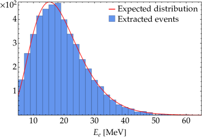
(a) IBD in Super-Kamiokande

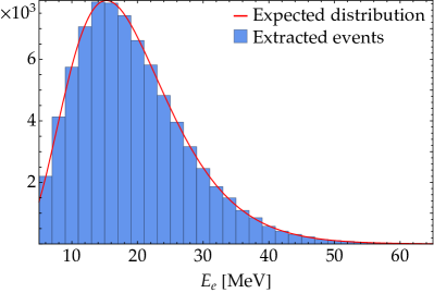
(b) IBD in Hyper-Kamiokande

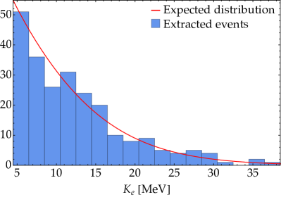
(c) ES in Super-Kamiokande

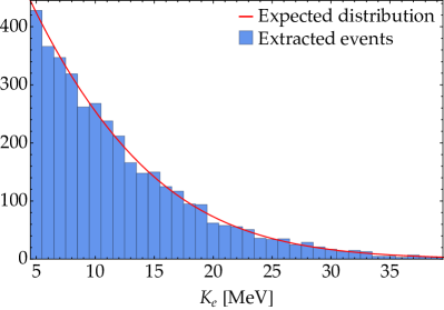
(d) ES in Hyper-Kamiokande

Figure 1: Extracted IBD (first row) and ES (second row) events used for the analysis in Super-Kamiokande (left column) and Hyper-Kamiokande (right column). The expected distributions, obtained by using eqs. (9) and (13) respectively, are plotted over the corresponding histograms.

2.3.2 Elastic scattering on electrons

Concerning the elastic scattering on electrons, the well-known tree level expression of the cross section — see e.g. refs. [10] or [49] — is

$$\frac{\mathrm{d}\sigma_{\mathrm{ES},j}}{\mathrm{d}y}=\frac{2G_{F}^{2}}{\pi}m_{e}E_{\nu}\left[g_{j}^{2}+g_{j}^{\prime 2}\left(1-y\right)^{2}-g_{j}g_{j}^{\prime}\frac{m_{e}}{E_{\nu}}y\right]\quad\mathrm{with}\quad j=\nu_{\mathrm{e}},\,\overline{\nu}_{\mathrm{e}},\,\nu_{\mu,\tau},\,\overline{\nu}_{\mu,\tau};$$ (11)

where $G_{F}$ is the Fermi constant, $m_{e}$ is the electron mass, $E_{\nu}$ the neutrino energy and $y$ is the electron kinetic energy $K_{e}=E_{e}-m_{e}$ over the neutrino energy

$$0<y=\frac{K_{e}}{E_{\nu}}<\left[1+\frac{m_{e}}{2E_{\nu}}\right]^{-1}.$$ (12)

The various a-dimensional constants are listed in table 3a.

By multiplying the cross section by the fluence (5) $\mathcal{F}_{i}\left(E_{\nu}\right)$ for each species and by the number $N_{e}$ of target electrons and by performing an integration, we end up with an analytical expression for the expected spectrum, differential in the kinetic energy of the recoiling electron

$$\mathscr{N}_{\text{ES}}\left(K_{e}\right)\equiv\frac{\text{dN}_{\text{ES}}}{\mathrm{d}{K_{e}}}=\sum_{\nu=\nu_{\mathrm{e}},\overline{\nu}_{\mathrm{e}},\nu_{x}} \xi_{\nu}\left[\left(G_{1\nu}+G_{2\nu}\right)\mathscr{F}_{\nu}^{(+1)}-2\frac{K_{e}}{T_{\nu}}G_{2\nu}\mathscr{F}_{\nu}^{(0)}\right.$$ (13)

$$\left.+\frac{K_{e}}{T_{\nu}}\left(\frac{K_{e}}{T_{\nu}}G_{2\nu}-\frac{m_{e}}{T_{\nu}}G_{3\nu}\right)\mathscr{F}_{\nu}^{(-1)}\right],$$

where $T_{\nu}$ is the same as (2) and the quantity $\xi_{\nu}$ is given by

$$\xi_{\nu}=\frac{2G_{F}^{2}m_{e}}{\pi}\frac{\mathcal{E}_{\nu}}{\langle E_{\nu}\rangle}\frac{N_{e}}{4\pi D^{2}}.$$ (14)

Functions $\mathscr{F}_{\nu}^{(i)}\left(K_{e}\right)$ are defined as follows

$$\mathscr{F}_{\nu}^{(i)}\left(K_{e}\right)=\frac{\Gamma\left(\alpha_{\nu}+i,(\zeta+1)K_{e}/T_{\nu}\right)}{\Gamma\left(\alpha_{\nu}+1\right)}\quad\text{with}\quad\zeta=\frac{m_{e}/K_{e}}{1+\sqrt{1+2m_{e}/K_{e}}},$$ (15)

where $\Gamma\left(a,z\right)$ is the incomplete gamma function

$$\Gamma(a,z)=\int_{z}^{\infty}e^{-t}\;t^{a-1}\;\mathrm{d}t.$$ (16)

Finally, the values of the numerical constants $G_{j\nu}$ are listed in table 3b.

Integrating eq. (13) from the threshold of $K_{e,\mathrm{thr}}=$5\text{\,}\mathrm{MeV}$-m_{e}$ that is identical for Super-Kamiokande and Hyper-Kamiokande, we obtain the number of expected ES events, $\mathrm{N}^{*}_{\mathrm{ES}}$, for the priors shown in table 1. The expected quantities are reported in the second row of table 2, together with the randomly extracted number of events considered in the present analysis. Each one of the ES events is characterized by a recoiling energy $K_{e}$, randomly distributed according to (13). The corresponding event distributions are plotted in figures 1c and 1d for Super-Kamiokande and Hyper-Kamiokande respectively.

	$g\rule{0.0pt}{11.19443pt}$	$g^{\prime}\rule[-5.16663pt]{0.0pt}{0.0pt}$
$\nu_{\mathrm{e}}\rule{0.0pt}{11.19443pt}$	$\frac{1}{2}+\sin^{2}\theta_{W}$	$\sin^{2}\theta_{W}$
$\overline{\nu}_{\mathrm{e}}$	$\sin^{2}\theta_{W}$	$\frac{1}{2}+\sin^{2}\theta_{W}$
$\nu_{\mu,\tau}$	$-\frac{1}{2}+\sin^{2}\theta_{W}$	$\sin^{2}\theta_{W}$
$\overline{\nu}_{\mu,\tau}\rule[-5.16663pt]{0.0pt}{0.0pt}$	$\sin^{2}\theta_{W}$	$-\frac{1}{2}+\sin^{2}\theta_{W}$

(a) Constants in (11)

$G_{j\nu}$	1	2	3
$\nu_{\mathrm{e}}$	0.073	0.054	-0.062
$\overline{\nu}_{\mathrm{e}}$	0.054	0.394	0.099
$\nu_{x}$	0.713	0.393	0.053

(b) Constants in (13)

Table 3: Numerical constants used in eqs. (11) (left table) and (13) (right table). The parameter $\theta_{W}$ is the Weinberg weak-mixing angle.

2.3.3 Neutral current neutrino-oxygen scattering

In order to compute the number of events due to neutrino interactions on ¹⁶O followed by gamma emission we take for the cross section the parametrization

$$\sigma_{\mathrm{OS}}(E_{\nu})\approx\sigma_{0}\left(E_{\nu}/$\mathrm{MeV}$-15\right)^{4}\vartheta\left(E_{\nu}/$\mathrm{MeV}$-15\right),$$ (17)

where $E_{\nu}$ is the energy of the incoming neutrino and $\vartheta$ the Heaviside theta function. The coefficient $\sigma_{0}$ is different for neutrinos or antineutrinos. We will refer to it as $\sigma_{0\nu}$ and $\sigma_{0\bar{\nu}}$ respectively. The expression (17) has proposed by ref. [36] to parametrize the cross sections computed with a microscopic approach.

In order to determine the value of $\sigma_{0}$, we reproduce the flux-averaged cross sections of ref. [38] (table I), shown in table 4. These have been obtained by folding the numerically computed cross sections $\sigma^{*}$

$$\sigma_{tot}=\int_{0}^{\infty}f_{FD}\left(E_{\nu}\middle|T,\,\mu\right)\sigma^{*}(E_{\nu})\mathrm{d}{E_{\nu}}.$$ (18)

with a pinched Fermi-Dirac spectrum $f_{FD}$

$$f_{FD}\left(E\right)=\left[T^{3}\,\tilde{F}_{2}\left(\frac{\mu}{T}\right)\right]^{-1}\frac{E^{2}}{1+\exp\left[\left(E-\mu\right)/T\right]},$$ (19)

where $\tilde{F}_{n}\left(\eta\right)$ is the Fermi integral of order $n$

$$\tilde{F}_{n}(\eta)=\int_{0}^{\infty}\frac{x^{n}\mathrm{d}x}{1+\exp\left(x-\eta\right)}.$$ (20)

For each process shown in the table and spectrum, we describe the numerical cross sections $\sigma^{*}$ with the expression given in eq. (17). We carry out two calculations with two different neutrino spectra referred to as $f_{FD,1}$ and $f_{FD,2}$. For the first case, the temperature is $T=$8\text{\,}\mathrm{MeV}$$ and the chemical potential $\mu=0$; while the second the spectrum is characterized by $T=$6.26\text{\,}\mathrm{MeV}$$ and $\mu=3T$.

$$f_{FD,1}\begin{cases}\sigma_{0\nu,1}=$4.08\text{\times}{10}^{-22}\text{\,}{\mathrm{fm}}^{2}$\\ \sigma_{0\bar{\nu},1}=$3.14\text{\times}{10}^{-22}\text{\,}{\mathrm{fm}}^{2}$\\ \end{cases}\qquad f_{FD,2}\begin{cases}\sigma_{0\nu,2}=$4.33\text{\times}{10}^{-22}\text{\,}{\mathrm{fm}}^{2}$\\ \sigma_{0\bar{\nu},2}=$3.52\text{\times}{10}^{-22}\text{\,}{\mathrm{fm}}^{2}$\\ \end{cases}.$$ (21)

Since for each spectrum we have two different values, the parameters taken as reference are a mean between $\sigma_{0\nu,1}$ and $\sigma_{0\nu,2}$ or between $\sigma_{0\bar{\nu},1}$ and $\sigma_{0\bar{\nu},2}$

$$\sigma_{0\nu}=$4.21\text{\times}{10}^{-22}\text{\,}{\mathrm{fm}}^{2}$\quad\text{and}\quad\sigma_{0,\bar{\nu}}=$3.33\text{\times}{10}^{-22}\text{\,}{\mathrm{fm}}^{2}$.$$ (22)

	Neutrinos		Antineutrinos
	Reaction	$\sigma_{tot}$	Reaction	$\sigma_{tot}$
		$(10^{-16}${\mathrm{fm}}^{2}$)$		$(10^{-16}${\mathrm{fm}}^{2}$)$
$f_{FD,1}$	$\mathrm{\textsuperscript{16}O}(\nu,\nu^{\prime}\mathrm{p}\gamma)\mathrm{\textsuperscript{15}N}$	1.41	$\mathrm{\textsuperscript{16}O}(\bar{\nu},\bar{\nu}^{\prime}\mathrm{p}\gamma)\mathrm{\textsuperscript{15}N}$	1.09
	$\mathrm{\textsuperscript{16}O}(\nu,\nu^{\prime}\mathrm{n}\gamma)\mathrm{\textsuperscript{15}O}$	0.37	$\mathrm{\textsuperscript{16}O}(\bar{\nu},\bar{\nu}^{\prime}\mathrm{n}\gamma)\mathrm{\textsuperscript{15}O}$	0.28
$f_{FD,2}$	$\mathrm{\textsuperscript{16}O}(\nu,\nu^{\prime}\mathrm{p}\gamma)\mathrm{\textsuperscript{15}N}$	0.72	$\mathrm{\textsuperscript{16}O}(\bar{\nu},\bar{\nu}^{\prime}\mathrm{p}\gamma)\mathrm{\textsuperscript{15}N}$	0.59
	$\mathrm{\textsuperscript{16}O}(\nu,\nu^{\prime}\mathrm{n}\gamma)\mathrm{\textsuperscript{15}O}$	0.18	$\mathrm{\textsuperscript{16}O}(\bar{\nu},\bar{\nu}^{\prime}\mathrm{n}\gamma)\mathrm{\textsuperscript{15}O}$	0.14

Table 4: Flux-averaged $\nu$-¹⁶O cross sections eq. (18) followed by $\gamma$ emission (from table I of ref. [38]). These are obtained by folding the numerical cross sections $\sigma^{*}$ with two different pinched Fermi-Dirac spectra. The first one, $f_{FD,1}$, has temperature $T=$8\text{\,}\mathrm{MeV}$$ and chemical potential $\mu=0$. The second one, $f_{FD,2}$, is characterized by $T=$6.26\text{\,}\mathrm{MeV}$$ and $\mu=3T$. Note that the cross sections are computed using a microscopic calculation.

The analytical expression is known to have an uncertainty of $\sim 10\%$ [36] that we have to take into account in the likelihood analysis. In order to do so, we introduce a tenth parameter, $\kappa$, as a multiplicative constant for the whole cross section (identical for neutrinos and antineutrinos). The final expression becomes

$$\sigma_{\mathrm{OS}}\left(E_{\nu}\right)=\kappa\,\sigma_{0,\nu}\left(E_{\nu}/$\mathrm{MeV}$-15\right)^{4}\vartheta\left(E_{\nu}/$\mathrm{MeV}$-15\right)$$ (23)

for neutrinos and similarly for antineutrinos (by replacing $\sigma_{0,\nu}$ with $\sigma_{0,\bar{\nu}}$). We assume the true value of $\kappa$ to be

$$\kappa^{*}=1$$ (24)

and vary it according to a gaussian distribution of mean 1 and variance

$$\sigma_{\kappa}=0.1.$$ (25)

This uncertainty reflects the $10\%$ precision on the cross section hopefully reachable in the future. Although it may seem quite optimistic in comparison with the available theoretical predictions in the literature (see e.g. refs. [50, 51, 38, 52]) we anticipate that the results depend only weakly on the inclusion of the NCR reactions. Note that even if the numerical neutrino-oxygen cross sections were employed, one should nevertheless include the corresponding current theoretical uncertainty. Moreover, as discussed in ref. [24], variations of $\kappa$ and $\sigma_{\kappa}$ parameters lead only to negligible changes.

In order to obtain the number of expected OS events, we have multiplied eq. (23) by the fluence $\mathcal{F}_{i}\left(E_{\nu}\right)$ and the number $N_{\rm O}$ of oxygen nuclei. Then, integrating on the neutrino energy, we end up with the number of expected OS events for the parameters described in table 1. Results are given in table 2 for both Super-Kamiokande and Hyper-Kamiokande. We recall that the quantity used in our analysis is the total amount of events in the NCR region, obtained by adding the IBD and ES background events with the OS signal events in the OS signal window (see section 2.1). The expected number of NCR events as well as the random quantities extracted for our analysis are also shown in table 2.

2.4 Likelihoods

Range [MeV]	$\Delta\left.E_{e}\right|_{\text{bin}}$ [MeV]
$5\leq E_{e}\leq 40$	0.5	$\Rightarrow$ 70 bins
$40\leq E_{e}\leq 50$	1	$\Rightarrow$ 10 bins
$50\leq E_{e}\leq 56$	2	$\Rightarrow$ 3 bins
$56\leq E_{e}\leq 60$	4	$\Rightarrow$ 1 bin
$60\leq E_{e}\leq 100$	40	$\Rightarrow$ 1 bin

Table 5: Bin widths (second column) used in IBD and ES likelihoods as a function of positron/electron energy ranges (first column). The number of bins used in each energy range is also shown (third column).

In order to analyze the IBD and ES extracted events, we use a binned likelihood

$$\mathcal{L}_{j}\left(\text{param.}\right)\propto\prod_{i=1}^{N_{\text{bin}}}\frac{\nu_{i}^{n_{i}}}{n_{i}}e^{-\nu_{i}}\quad\text{with}\>j=\text{IBD, ES};$$ (26)

where $\nu_{i}$ is the number of expected events for the process $j$ (as a function of parameters) in the $i$-th bin and $n_{i}$ is the number observed in the simulation, in the same bin. Bin widths are not uniform, but vary according to table 5, so as to preserve the relevant features of the distributions. The same choice is adopted in refs. [21, 24].

Concerning the neutral current events on oxygen, the likelihood form would be in principle simply Poissonian, since we have to compare the number of expected events $\text{N}_{\mathrm{NCR}}$ (as a function of the parameters) with the extracted one $n_{\mathrm{NCR}}$. Nevertheless, we have also to take into account the uncertainty on the cross section via the $\kappa$ parameter eq. (23–24). Therefore, the likelihood expression becomes

$$\mathcal{L}_{\mathrm{NCR}}\left(\text{param.}\right)=\left(2\pi\text{N}_{\mathrm{NCR}}2\pi\sigma_{\kappa}^{2}\right)^{-1/2}\exp\left[-\frac{\left(n_{\mathrm{NCR}}-\text{N}_{\mathrm{NCR}}\right)^{2}}{2\text{N}_{\mathrm{NCR}}}-\frac{\left(\kappa-1\right)^{2}}{2\sigma_{\kappa}^{2}}\right].$$ (27)

In order to quantify the relevance of the various reactions in the reconstruction of the emission parameters, we apply the same strategy as in ref. [24] and perform three different analyses, for Super-Kamiokande and Hyper-Kamiokande separately. First we perform an analysis with IBD events alone. Then a second one where we add the ES information. Finally the third one exploits IBD, ES and NCR. In the three analysis we assume 100% tagging efficiency for IBD and ES processes above $5\text{\,}\mathrm{MeV}$ (see section 2.1). Thus, for each analysis the global likelihood is expressed as the product of the likelihoods of the single processes.

As in ref. [24], a Monte Carlo approach is employed: each variable is free to vary inside the corresponding prior (table 1). Then, the $n-$dimensional region described by these priors is covered with random points $P$. Each of them is accepted within a certain confidence level (CL) if its likelihood satisfies the relation

$$\log\mathcal{L}\left(P\right)\geq\log\mathcal{L}_{max}-\frac{A}{2},$$ (28)

where $\mathcal{L}_{max}$ is the likelihood maximum inside the prior and $A$ is defined with an integral of a chi-square distribution with $N_{\mathrm{dof}}$ degrees of freedom

$$\int_{0}^{A}\chi^{2}(N_{\mathrm{dof}};z)\,\mathrm{d}{z}=\mathrm{CL},$$ (29)

For instance, considering $\mathrm{CL}=0.9973$, namely $3\sigma$, we find $A=11.8292,\,18.2053,\,26.9011$ for $N_{\mathrm{dof}}=2,\,5,\,10$ respectively.

Before performing our main analysis including the three detection channels, we have validated our method by reproducing the results of ref. [21] where a 6 degrees of freedom statistical analysis of the IBD events in Hyper-Kamiokande is performed. By assuming the same fluxes and choice of the parameters as in ref. [21] we have extracted 30k 6-dimensional points in the parameter space, accepted within the same confidence level, i.e. $2\sigma$. Our projected results into various two-dimensional planes are plotted in figure 2. As one can see by comparing figure 2 with figure 4 of ref. [21], there is full compatibility between our results and those obtained by likelihood marginalization.

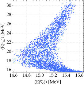
(a) $\langle E_{\overline{\nu}_{\!\;\!\mbox{\tiny e}}}\rangle$–$\langle E_{\nu_{\mbox{\tiny$x$}}}\rangle$ projection

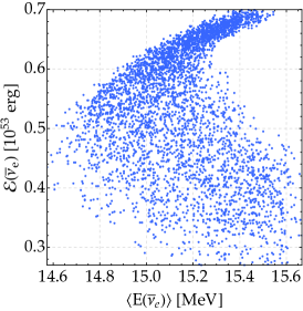
(b) $\langle E_{\overline{\nu}_{\!\;\!\mbox{\tiny e}}}\rangle$–$\mathcal{E}_{\overline{\nu}_{\!\;\!\mbox{\tiny e}}}$ projection

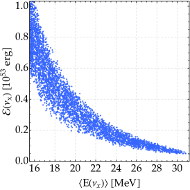
(c) $\langle E_{\nu_{\mbox{\tiny$x$}}}\rangle$–$\mathcal{E}_{\nu_{\mbox{\tiny$x$}}}$ projection

Figure 2: Results of the 6 degrees of freedom likelihood analysis based on IBD events in Hyper-Kamiokande. In order to compare our findings with those of ref. [21] (figure 4) we make the same hypotheses but employ the Monte Carlo method described in the text. The results shown correspond to a subset of the 6-dimensional parameter space that is accepted at $2\sigma$ CL and projected onto: the $\langle E_{\overline{\nu}_{\!\;\!\mbox{\tiny e}}}\rangle$–$\langle E_{\nu_{\mbox{\tiny$x$}}}\rangle$ plane LABEL:sub@fig:mik1, $\langle E_{\overline{\nu}_{\!\;\!\mbox{\tiny e}}}\rangle$–$\mathcal{E}_{\overline{\nu}_{\!\;\!\mbox{\tiny e}}}$ LABEL:sub@fig:mik2, and $\langle E_{\nu_{\mbox{\tiny$x$}}}\rangle$–$\mathcal{E}_{\nu_{\mbox{\tiny$x$}}}$ LABEL:sub@fig:mik3. The prior for $\mathcal{E}_{i}$ is $[0.2,\,1.2]\times 10^{53}$ erg while for $\langle E_{i}\rangle$ is $[8,\,32]$ MeV.

3 Reconstruction of the neutrino spectra: numerical results

Our analyses are performed extracting 30k points for each of the three dataset: IBD, IBD+ES, IBD+ES+NCR. Then, the points are projected onto selected 2-dimensional and 1-dimensional regions, obtaining the distributions for the parameters defining the neutrino spectra, whose description and study constitute the aim of this section.

3.1 Total and partial neutrino luminosities

Given an extracted point $P$, the total emitted energy can be reconstructed as

$$\mathcal{E}_{\mathrm{B},P}=\mathcal{E}_{\nu_{\mbox{\tiny e}},P}+\mathcal{E}_{\overline{\nu}_{\!\;\!\mbox{\tiny e}},P}+4\mathcal{E}_{\nu_{\mbox{\tiny$x$}},P}.$$ (30)

As can be seen from figure 3 the energy emitted in electron neutrinos cannot be determined from the IBD-only analysis and remains randomly distributed inside the prior. From the latter we extract its value in order to determine $\mathcal{E}_{\mathrm{B}}$. The corresponding values for each extracted point can be gathered in a histogram. Figure 3 shows the results for Hyper-Kamiokande, without LABEL:sub@fig:EtotSt and with LABEL:sub@fig:EtotEq the equipartition ansatz. Note that the ones for Super-Kamiokande have been published elsewhere (see figure 1 of ref. [24]).

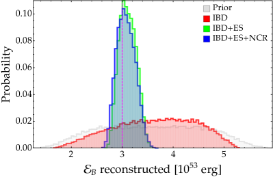
(a) Hyper-Kamiokande (standard)

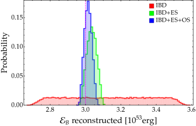
(b) Hyper-Kamiokande (equipartition)

Figure 3: One-dimensional projection of the total emitted energy $\mathcal{E}_{\mathrm{B}}$ reconstructed in Hyper-Kamiokande from sets of 30k extracted points at $3\sigma$ CL using (30). The results correspond to the analysis either without any constraints LABEL:sub@fig:EtotSt or with the equipartition ansatz LABEL:sub@fig:EtotEq. The different colors refer to the three analyses with increasing information through the number of included channels. The gray distribution is the prior one, obtained by extracting $\mathcal{E}_{\nu_{\mbox{\tiny e}}}$, $\mathcal{E}_{\overline{\nu}_{\!\;\!\mbox{\tiny e}}}$, $\mathcal{E}_{\nu_{\mbox{\tiny$x$}}}$ uniformly in the prior $[0.2,1]\times${10}^{53}\text{\,}\mathrm{erg}$$. The dashed magenta line marks the true value. Means and standard deviations of each histogram are reported in table 6.

One can see that the IBD-only analysis leads to a distribution for the binding energy that is almost identical to the one that follows simply by the choice of the priors. This result is in agreement with the conclusions drawn by Minakata et al. [21]. It is the inclusion of the other event samples (ES and NCR) that breaks the parameter degeneracy and allows us to determine the total emitted energy. This important conclusion differs qualitatively from the pessimistic one drawn in ref. [21]: it is possible to determine the total emitted energy, as first shown in ref. [24] for the case of Super-Kamiokande. In particular the accuracy of $\sim 11\%$ with Super-Kamiokande can be improved to $\sim 6\%$ in Hyper-Kamiokande.

		SUPER-KAMIOKANDE									HYPER-KAMIOKANDE
Param.	$\ast$	IBD			IBD+ES			IBD+ES+NCR			IBD			IBD+ES			IBD+ES+NCR
		Val.		%	Val.		%	Val.		%	Val.		%	Val.		%	Val.		%
$\rule{0.0pt}{11.19443pt}\mathcal{E}_{\mathrm{B}}\rule[-5.16663pt]{0.0pt}{0.0pt}[${10}^{53}\text{\,}\mathrm{erg}$]$	$3$	$3.40$${}\pm{}$	$0.86$	25	$3.27$${}\pm{}$	$0.37$	11	$3.18$${}\pm{}$	$0.35$	11	$3.64$${}\pm{}$	$0.79$	22	$3.11$${}\pm{}$	$0.16$	5.3	$3.07$${}\pm{}$	$0.18$	5.8	STANDARD
$\cdashline{1-20}\rule{0.0pt}{11.19443pt}\mathcal{E}_{\nu_{\mbox{\tiny e}}}\rule[-5.16663pt]{0.0pt}{0.0pt}[${10}^{53}\text{\,}\mathrm{erg}$]$	$0.5$	—			$0.60$${}\pm{}$	$0.23$	39	$0.57$${}\pm{}$	$0.23$	41	—			$0.57$${}\pm{}$	$0.23$	40	$0.56$${}\pm{}$	$0.23$	41
$\rule{0.0pt}{11.19443pt}\mathcal{E}_{\overline{\nu}_{\!\;\!\mbox{\tiny e}}}\rule[-5.16663pt]{0.0pt}{0.0pt}[${10}^{53}\text{\,}\mathrm{erg}$]$	$0.5$	$0.48$${}\pm{}$	$0.11$	22	$0.493$${}\pm{}$	$0.051$	10	$0.490$${}\pm{}$	$0.050$	10	$0.442$${}\pm{}$	$0.094$	21	$0.504$${}\pm{}$	$0.017$	3.3	$0.503$${}\pm{}$	$0.018$	3.6
$\rule{0.0pt}{11.19443pt}\mathcal{E}_{\nu_{\mbox{\tiny$x$}}}\rule[-5.16663pt]{0.0pt}{0.0pt}[${10}^{53}\text{\,}\mathrm{erg}$]$	$0.5$	$0.58$${}\pm{}$	$0.23$	40	$0.55$${}\pm{}$	$0.10$	18	$0.53$${}\pm{}$	$0.09$	18	$0.65$${}\pm{}$	$0.21$	33	$0.508$${}\pm{}$	$0.035$	6.9	$0.503$${}\pm{}$	$0.037$	7.4
$\cdashline{1-20}\rule{0.0pt}{11.19443pt}\langle E_{\nu_{\mbox{\tiny e}}}\rangle\rule[-5.16663pt]{0.0pt}{0.0pt}[$\mathrm{MeV}$]$	$9.5$	—			$17.6$${}\pm{}$	$6.9$	39	$14.0$${}\pm{}$	$5.3$	38	—			$12.4$${}\pm{}$	$4.5$	36	$11.0$${}\pm{}$	$4.0$	33
$\rule{0.0pt}{11.19443pt}\langle E_{\overline{\nu}_{\!\;\!\mbox{\tiny e}}}\rangle\rule[-5.16663pt]{0.0pt}{0.0pt}[$\mathrm{MeV}$]$	$12$	$12.9$${}\pm{}$	$1.6$	12	$11.86$${}\pm{}$	$0.82$	6.9	$11.99$${}\pm{}$	$0.73$	6.1	$12.8$${}\pm{}$	$1.3$	10	$11.94$${}\pm{}$	$0.26$	2.2	$11.98$${}\pm{}$	$0.27$	2.3
$\rule{0.0pt}{11.19443pt}\langle E_{\nu_{\mbox{\tiny$x$}}}\rangle\rule[-5.16663pt]{0.0pt}{0.0pt}[$\mathrm{MeV}$]$	$15.6$	$12.1$${}\pm{}$	$2.9$	24	$14.4$${}\pm{}$	$1.7$	12	$14.6$${}\pm{}$	$1.6$	11	$13.5$${}\pm{}$	$2.0$	15	$15.4$${}\pm{}$	$1.1$	7.0	$15.7$${}\pm{}$	$1.1$	6.9
$\cdashline{1-20}\rule{0.0pt}{11.19443pt}\alpha_{\nu_{\mbox{\tiny e}}}\rule[-5.16663pt]{0.0pt}{0.0pt}$	$2.5$	—			$2.52$${}\pm{}$	$0.58$	23	$2.56$${}\pm{}$	$0.57$	22	—			$2.54$${}\pm{}$	$0.57$	23	$2.56$${}\pm{}$	$0.57$	22
$\alpha_{\overline{\nu}_{\!\;\!\mbox{\tiny e}}}\rule[-5.16663pt]{0.0pt}{0.0pt}$	$2.5$	$2.36$${}\pm{}$	$0.51$	22	$2.13$${}\pm{}$	$0.41$	19	$2.22$${}\pm{}$	$0.44$	20	$2.39$${}\pm{}$	$0.40$	17	$2.45$${}\pm{}$	$0.15$	6.0	$2.53$${}\pm{}$	$0.17$	6.9
$\rule{0.0pt}{11.19443pt}\alpha_{\nu_{\mbox{\tiny$x$}}}\rule[-5.16663pt]{0.0pt}{0.0pt}$	$2.5$	$2.47$${}\pm{}$	$0.57$	23	$2.53$${}\pm{}$	$0.56$	22	$2.59$${}\pm{}$	$0.55$	21	$2.63$${}\pm{}$	$0.50$	19	$2.44$${}\pm{}$	$0.42$	17	$2.57$${}\pm{}$	$0.44$	17
$\cdashline{1-20}\rule{0.0pt}{11.19443pt}\kappa\rule[-5.16663pt]{0.0pt}{0.0pt}$	$1$	—			—			$0.99$${}\pm{}$	$0.11$	11	—			—			$0.90$${}\pm{}$	$0.06$	6.3
$\rule{0.0pt}{11.19443pt}\mathcal{E}_{\mathrm{B}}\rule[-5.16663pt]{0.0pt}{0.0pt}[${10}^{53}\text{\,}\mathrm{erg}$]$	$3$	$3.15$${}\pm{}$	$0.25$	7.9	$3.06$${}\pm{}$	$0.10$	3.4	$3.023$${}\pm{}$	$0.095$	3.1	$3.13$${}\pm{}$	$0.23$	7.4	$3.035$${}\pm{}$	$0.027$	0.89	$3.015$${}\pm{}$	$0.021$	0.68	EQUIPARTITION
$\cdashline{1-20}\rule{0.0pt}{11.19443pt}\mathcal{E}_{\nu_{\mbox{\tiny e}}}\rule[-5.16663pt]{0.0pt}{0.0pt}[${10}^{53}\text{\,}\mathrm{erg}$]$	$0.5$	—			$0.511$${}\pm{}$	$0.017$	3.4	$0.504$${}\pm{}$	$0.016$	3.1	—			$0.5059$${}\pm{}$	$0.0045$	0.89	$0.5025$${}\pm{}$	$0.0034$	0.68
$\rule{0.0pt}{11.19443pt}\mathcal{E}_{\overline{\nu}_{\!\;\!\mbox{\tiny e}}}\rule[-5.16663pt]{0.0pt}{0.0pt}[${10}^{53}\text{\,}\mathrm{erg}$]$	$0.5$	$0.511$${}\pm{}$	$0.019$	3.7	$0.511$${}\pm{}$	$0.017$	3.4	$0.504$${}\pm{}$	$0.016$	3.1	$0.5057$${}\pm{}$	$0.0047$	0.92	$0.5059$${}\pm{}$	$0.0045$	0.89	$0.5025$${}\pm{}$	$0.0034$	0.68
$\rule{0.0pt}{11.19443pt}\mathcal{E}_{\nu_{\mbox{\tiny$x$}}}\rule[-5.16663pt]{0.0pt}{0.0pt}[${10}^{53}\text{\,}\mathrm{erg}$]$	$0.5$	$0.511$${}\pm{}$	$0.019$	3.7	$0.511$${}\pm{}$	$0.017$	3.4	$0.504$${}\pm{}$	$0.016$	3.1	$0.5057$${}\pm{}$	$0.0047$	0.92	$0.5059$${}\pm{}$	$0.0045$	0.89	$0.5025$${}\pm{}$	$0.0034$	0.68
$\cdashline{1-20}\rule{0.0pt}{11.19443pt}\langle E_{\nu_{\mbox{\tiny e}}}\rangle\rule[-5.16663pt]{0.0pt}{0.0pt}[$\mathrm{MeV}$]$	$9.5$	—			$17.9$${}\pm{}$	$6.9$	39	$14.3$${}\pm{}$	$5.2$	37	—			$12.8$${}\pm{}$	$4.4$	34	$10.6$${}\pm{}$	$3.0$	28
$\rule{0.0pt}{11.19443pt}\langle E_{\overline{\nu}_{\!\;\!\mbox{\tiny e}}}\rangle\rule[-5.16663pt]{0.0pt}{0.0pt}[$\mathrm{MeV}$]$	$12$	$13.0$${}\pm{}$	$1.4$	11	$11.72$${}\pm{}$	$0.68$	5.8	$11.92$${}\pm{}$	$0.65$	5.4	$12.59$${}\pm{}$	$0.81$	6.5	$11.92$${}\pm{}$	$0.26$	2.2	$11.94$${}\pm{}$	$0.21$	1.7
$\rule{0.0pt}{11.19443pt}\langle E_{\nu_{\mbox{\tiny$x$}}}\rangle\rule[-5.16663pt]{0.0pt}{0.0pt}[$\mathrm{MeV}$]$	$15.6$	$12.1$${}\pm{}$	$2.8$	23	$14.8$${}\pm{}$	$1.6$	11	$14.8$${}\pm{}$	$1.5$	10	$13.7$${}\pm{}$	$2.1$	16	$15.4$${}\pm{}$	$1.0$	6.5	$15.84$${}\pm{}$	$0.80$	5.0
$\cdashline{1-20}\rule{0.0pt}{11.19443pt}\alpha_{\nu_{\mbox{\tiny e}}}\rule[-5.16663pt]{0.0pt}{0.0pt}$	$2.5$	—			$2.52$${}\pm{}$	$0.58$	23	$2.55$${}\pm{}$	$0.57$	22	—			$2.54$${}\pm{}$	$0.57$	23	$2.57$${}\pm{}$	$0.57$	22
$\alpha_{\overline{\nu}_{\!\;\!\mbox{\tiny e}}}\rule[-5.16663pt]{0.0pt}{0.0pt}$	$2.5$	$2.35$${}\pm{}$	$0.52$	22	$2.09$${}\pm{}$	$0.39$	18	$2.20$${}\pm{}$	$0.43$	20	$2.25$${}\pm{}$	$0.32$	14	$2.44$${}\pm{}$	$0.16$	6.4	$2.53$${}\pm{}$	$0.13$	5.3
$\rule{0.0pt}{11.19443pt}\alpha_{\nu_{\mbox{\tiny$x$}}}\rule[-5.16663pt]{0.0pt}{0.0pt}$	$2.5$	$2.48$${}\pm{}$	$0.57$	23	$2.61$${}\pm{}$	$0.55$	21	$2.63$${}\pm{}$	$0.55$	21	$2.80$${}\pm{}$	$0.51$	18	$2.46$${}\pm{}$	$0.40$	16	$2.61$${}\pm{}$	$0.34$	13
$\cdashline{1-20}\rule{0.0pt}{11.19443pt}\kappa\rule[-5.16663pt]{0.0pt}{0.0pt}$	$1$	—			—			$0.99$${}\pm{}$	$0.11$	11	—			—			$0.953$${}\pm{}$	$0.098$	10

Table 6: Reconstruction of the emission parameters in Super-Kamiokande (left block) and Hyper-Kamiokande (right block), without (top rows) and with (bottom rows) equipartition ansatz. Considerations on the emission parameters can be found in section 2.2. The three analyses differ for the number of detection channels included: IBD, IBD+ES, IBD+ES+NCR (see section 2.3). The $\kappa$ parameter takes into account the theoretical uncertainty on the neutral current neutrino-oxygen cross section (see section 2.2). In each cell we report mean, standard deviation and percentage accuracy obtained from 30k extracted random points accepted at $3\sigma$ CL. The second column marked by the asterisk reports the true values of the emission parameters used in the analysis.

If an exact equipartition held true, Super-Kamiokande would be able to reach a precision of few percent while Hyper-Kamiokande could reconstruct the total energy with an accuracy less than $1\%$ — namely $0.7\%$. Let us repeat that the hypothesis of an exact equipartition nowadays should be regarded as a very aggressive assumption, since current simulations indicate that it should hold true only within a factor of 2 (see e.g. refs. [40, 45, 46]).

A way of representing the fraction of the total energy carried out by each species is by plotting the reconstructed emitted energies per flavor on a ternary diagram. This is shown in figure 4a for Super-Kamiokande and figure 4b for Hyper-Kamiokande. As one can see the ternary diagrams are not much instructive since the points are distributed over the whole region.

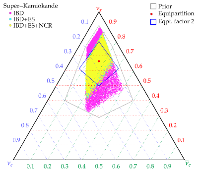
(a) Super-Kamiokande

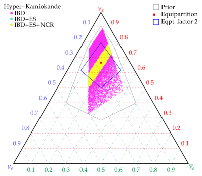
(b) Hyper-Kamiokande

Figure 4: Ternary plot for Super-Kamiokande LABEL:sub@fig:skter and Hyper-Kamiokande LABEL:sub@fig:hkter where the three axes correspond to the amount of $\mathcal{E}_{\nu_{\mbox{\tiny e}}}$, $\mathcal{E}_{\overline{\nu}_{\!\;\!\mbox{\tiny e}}}$ and $4\mathcal{E}_{\nu_{\mbox{\tiny$x$}}}$ for each extracted point. Different colors represent the three analyses performed with increasing information gained through the addition of detection channels. The gray line marks the allowed a priori region, obtained extracting $\mathcal{E}_{\nu_{\mbox{\tiny e}}}$, $\mathcal{E}_{\overline{\nu}_{\!\;\!\mbox{\tiny e}}}$, $\mathcal{E}_{\nu_{\mbox{\tiny$x$}}}$ uniformly in the prior $[0.2,1]\times${10}^{53}\text{\,}\mathrm{erg}$$. The blue line, on the other hand contains the points for which the equipartition hypothesis holds true within a factor of 2. The red dot indicates the value corresponding to the equipartition ansatz. Each set contains 30k extracted points at $3\sigma$ CL.

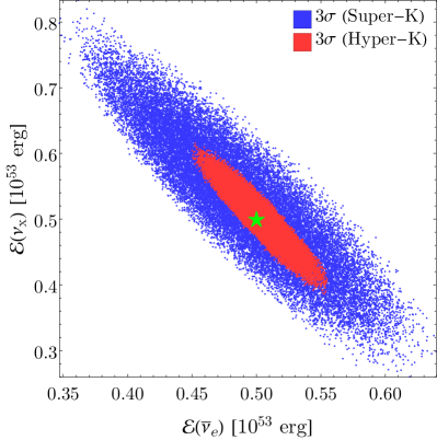
(a) IBD+ES+NCR

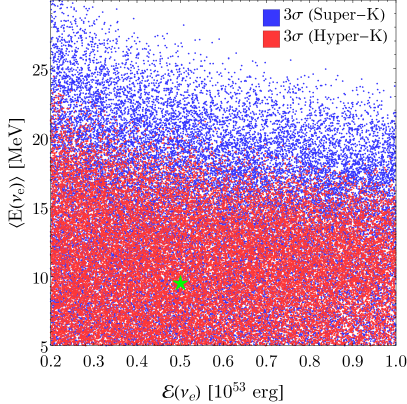
(b) IBD+ES+NCR

Figure 5: Projection of the extracted points onto the $\mathcal{E}_{\overline{\nu}_{\!\;\!\mbox{\tiny e}}}$–$\mathcal{E}_{\nu_{\mbox{\tiny$x$}}}$ plane LABEL:sub@fig:scate2 and $\mathcal{E}_{\nu_{\mbox{\tiny e}}}$–$\langle E_{\nu_{\mbox{\tiny e}}}\rangle$ LABEL:sub@fig:scate1 plane. The blue dots refer to Super-Kamiokande while the red ones to Hyper-Kamiokande. Each set contains 30k points, accepted at $3\sigma$ CL. The three detection channels have been considered. Notice that the prior for $\mathcal{E}_{i}$ is $[0.2,1]\times${10}^{53}\text{\,}\mathrm{erg}$$ and $[5,30]\,$\mathrm{MeV}$$ for $\langle E_{i}\rangle$. The green star marks the true value.

If we assume the factor of 2 of uncertainty is a reliable estimate, we can decrease the size of the region where the point are extracted, and keep only those that fall inside the blue line. This additional assumption, however, does not improve significantly the results obtained with the three-channels analysis. For instance, the three-channels analysis in Hyper-Kamiokande gives a total emitted energy of $\left(3.12\pm 0.15\right)\times${10}^{53}\text{\,}\mathrm{erg}$$, that corresponds to a slightly better accuracy ($\sim 5\%$) just because the reconstructed value is bigger.

The projected emitted energy for $\nu_{x}$ as a function of the $\overline{\nu}_{e}$ one is shown in figure 5. One can see that Hyper-Kamiokande will be able to measure the energy emitted in $\nu_{x}$ species (4 of them, out of 6) with an accuracy of $\sim 7\%$, instead of the $\sim 18\%$ that Super-Kamiokande should achieve (table 6). As for the $\overline{\nu}_{\mathrm{e}}$ the measurement of the corresponding (integrated) luminosity goes from $\sim 10\%$ in Super-Kamiokande to $\sim 4\%$ in Hyper-Kamiokande. The inclusion of the $\nu_{\mathrm{e}}$ and $\overline{\nu}_{\mathrm{e}}$ species to the $\nu_{x}$ ones leads to a slight decrease of the uncertainty on the total emitted energy, that has already mentioned, amounts to $5\%$.

Studying the total energy distributions for each neutrino flavor, we notice that the main source of uncertainties is attributable to the fact that no specific detection channel sensitive to electron neutrinos is added in the analysis. This can be seen from table 2 since the fraction of $\nu_{\mathrm{e}}$ events is small compared to the $\overline{\nu}_{\mathrm{e}}$ or $\nu_{x}$ ones. As a consequence, the reconstruction of the $\nu_{\mathrm{e}}$ emitted energy does not improve from Super-Kamiokande to Hyper-Kamiokande; the electron neutrino properties remain largely undetermined. This is true for the electron neutrino luminosity as well as for the mean energy and pinching parameter.

3.2 Mean energies and pinching

The mean energies of $\overline{\nu}_{\mathrm{e}}$ and $\nu_{x}$ can be precisely reconstructed. Their values are plotted in figure 6, for the two detectors and as a function of number of detection channels. The corresponding averages and standard deviations are reported in table 6. A precision of $\sim 2\%$ in Hyper-Kamiokande ($\sim 6\%$ in Super-Kamiokande) and $\sim 7\%$ in Hyper-Kamiokande ($\sim 11\%$ in Super-Kamiokande) can be reached for $\overline{\nu}_{\mathrm{e}}$ and $\nu_{x}$ respectively. Again, this result is achieved thanks to the combination of the main channels, i.e. inverse beta decay and neutrino elastic scattering on electrons. In fact, table 6 shows that IBD-only is not sufficient to determine precisely even the energy of the $\overline{\nu}_{\mathrm{e}}$, despite the high statistics (see table 2). The inclusion of elastic scattering interactions in the analysis improves strongly the outcome. As expected, the $\langle E_{\overline{\nu}_{\!\;\!\mbox{\tiny e}}}\rangle$ improves more than $\nu_{x}$ due to the higher percentage of survived $\overline{\nu}_{\mathrm{e}}$ after the MSW effect.

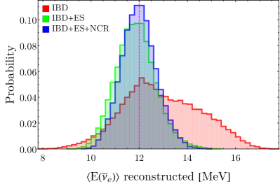
(a) $\langle E_{\overline{\nu}_{\!\;\!\mbox{\tiny e}}}\rangle$ in Super-Kamiokande

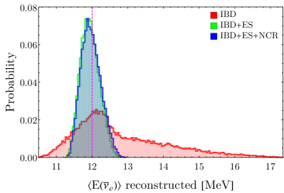
(b) $\langle E_{\overline{\nu}_{\!\;\!\mbox{\tiny e}}}\rangle$ in Hyper-Kamiokande

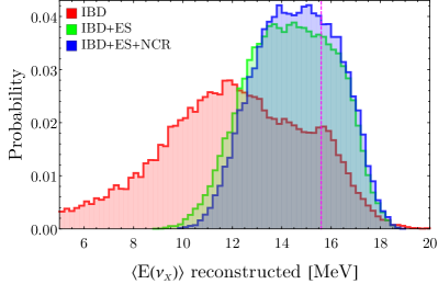
(c) $\langle E_{\nu_{\mbox{\tiny$x$}}}\rangle$ in Super-Kamiokande

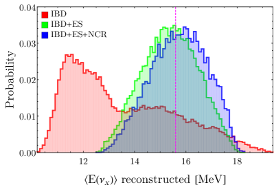
(d) $\langle E_{\nu_{\mbox{\tiny$x$}}}\rangle$ in Hyper-Kamiokande

Figure 6: Distributions of reconstructed $\langle E_{\overline{\nu}_{\!\;\!\mbox{\tiny e}}}\rangle$ (first row) and $\langle E_{\nu_{\mbox{\tiny$x$}}}\rangle$ (second row) in Super-Kamiokande (left) and Hyper-Kamiokande (right). Different colors represent the amount of information used through the number of detection channels. Each histogram contains 30k extracted points, accepted at $3\sigma$ CL. The dashed magenta line marks the true value. Means and standard deviations of those histograms are reported in table 6.

The reconstructed value of $\langle E_{\nu_{\mbox{\tiny$x$}}}\rangle$ in Super-Kamiokande turns out to be slightly below the expectations. While this is within the statistical uncertainty, one reason that favors this behavior is the flux parameters degeneracy, that allows an interplay between the normalization of the spectrum $\mathcal{E}_{\nu_{\mbox{\tiny$x$}}}$, its first momentum $\langle E_{\nu_{\mbox{\tiny$x$}}}\rangle$ and its width $\alpha_{\nu_{\mbox{\tiny$x$}}}$. For instance, in the analysis based on three detection channels, a slightly underestimated value of $\langle E_{\nu_{\mbox{\tiny$x$}}}\rangle$ corresponds to a slight overestimation of $\alpha_{\nu_{\mbox{\tiny$x$}}}$ and of $\mathcal{E}_{\nu_{\mbox{\tiny$x$}}}$.

The projected results for $\nu_{\mathrm{e}}$ on the $\mathcal{E}_{\nu_{\mbox{\tiny e}}}$–$\langle E_{\nu_{\mbox{\tiny e}}}\rangle$ plane are given in figure 4b. As one can see their distribution is almost uniform inside the prior. This shows that the $\nu_{\mathrm{e}}$ average energies are to large extent undetermined since $\langle E_{\nu_{\mbox{\tiny e}}}\rangle$ goes almost uniformly from 5 to $25\text{\,}\mathrm{MeV}$ for Super-Kamiokande and from 5 to $20\text{\,}\mathrm{MeV}$ for Hyper-Kamiokande.

As far as the pinching parameter is concerned, figure 7 shows the extracted points projected onto the $\alpha_{\nu_{\mbox{\tiny e}}}$–$\alpha_{\nu_{\mbox{\tiny$x$}}}$ plane. As one can see there, as well as in table 6, the pinching distribution in Super-Kamiokande is almost uniform inside the prior. Concerning Hyper-Kamiokande, the combination of the three detection channels allows to measure the pinching parameter of the $\overline{\nu}_{\mathrm{e}}$ species with a good accuracy ($\sim 7\%$). In fact this is expected: since the total and mean energy are quite well determined, there cannot be a large uncertainty on $\alpha_{\overline{\nu}_{\!\;\!\mbox{\tiny e}}}$.

Concerning $\alpha_{\nu_{\mbox{\tiny e}}}$, their values cover the prior range almost uniformly, and the $\sim 23\%$ precision is simply due to its choice. In fact, with a prior uniform in the interval $[1.5,3.5]$ we expect a mean of 2.5 and a standard deviation of $1/\sqrt{3}$ that corresponds to a prior accuracy at the level of 23%. Such a result is close to the outcomes of most available analyses, and is what we find in ours (see table 6). Clearly, to pin down the $\alpha_{\nu_{\mbox{\tiny e}}}$ value more channels sensitive to the electron neutrino spectrum should be added.

Finally, very similar conclusions on the average energies and the pinching follow even assuming that an exact equipartition of the neutrino emitted energies holds true. In fact, as one can see from table 6, the reconstructed values of the average energies and pinching parameters do not differ much without or with energy equipartition.

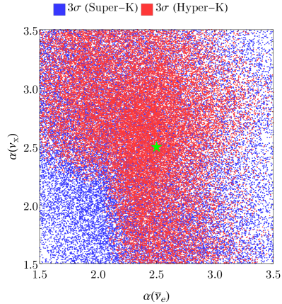
(a) IBD

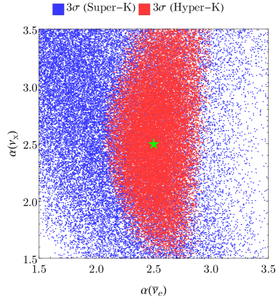
(b) IBD+ES+NCR

Figure 7: Projection of the extracted points onto the $\alpha_{\overline{\nu}_{\!\;\!\mbox{\tiny e}}}$–$\alpha_{\nu_{\mbox{\tiny$x$}}}$ plane, in the IBD-only analysis LABEL:sub@fig:scate3 and combining all the detection channels LABEL:sub@fig:scate4. The blue dots refer to Super-Kamiokande while the red ones to Hyper-Kamiokande. Each set contains 30k points, accepted at $3\sigma$ CL. The boundaries of the region are given by the prior $[1.5,3.5]$ — see section 2.2. The green star marks the true value.

4 Conclusions

In this manuscript we have focused on our ability to reconstruct the neutrino spectra of a galactic supernova in water Cherenkov detectors, i.e. Hyper-Kamiokande and Super-Kamiokande. Contrarily to most of the existing studies we have not imposed any constraint to the flux parameters. Also, we have combined here three detection channels, namely inverse beta decay, elastic scattering on electrons and neutral current scattering on oxygen. Our 10 degrees of freedom likelihood analyses have shown that the total and individual neutrino luminosities can be determined with a few percent precision, except for the electron neutrinos. In particular, the total emitted energy in Hyper-Kamiokande can be reconstructed within a few percent ($\sim 6\%$), that becomes less than $1\%$ in case the equipartition hypothesis holds true. Note that information about this hypothesis is hardly extractable from the data.

The average energies and pinching can also be identified at at few percent level while the electron neutrino ones remain undetermined. The best constrained by the analysis are the electron antineutrinos: their mean energy and pinching can be reconstructed up to $\sim 2\%$ and $\sim 7\%$ respectively in Hyper-Kamiokande. Such results are mainly due to combining information from inverse beta decay and elastic scattering. They are also particularly remarkable because of the absence of a priori choices of the flux parameters in the likelihoods.

The assumptions adopted in the present analysis can be extended in several ways. For what concerns the neutrino fluxes, we have assumed that they are given by quasi-thermal distributions, modified by the MSW effect in normal ordering. Other cases can be studied, for instance, those where the spectra undergo changes due to the neutrino self-interactions. Future more precise inputs from the numerical simulations for the fluxes and for their uncertainties are clearly highly desirable. On the other hand, more detectors and/or detection channels can be combined to those considered in the present work, especially for the aim of reconstructing precisely the electron neutrino fluxes, or for disposing of a clean sample of neutral current events. The investigation of these issues will be the object of future work.

The next (extra)galactic supernova is of great interest for astrophysics and particle physics. In particular, although the uncertainties on the neutrino fluxes are still large, this observation will bring crucial information on the explosion mechanism, through the neutrino light-curves, and on neutrino flavor conversion in the supernova, with the reconstruction of the energy spectra. Detailed investigations are needed to demonstrate that the neutrino flux uncertainties will not prevent us from extracting important information. The work presented here represents a supplementary step in this direction.

References

- [1] S. A. Colgate and M. H. Johnson, Phys. Rev. Lett. 5, 235 (1960).
- [2] S. A. Colgate and R. H. White, Astrophys. J. 143, 626 (1966).
- [3] J. Wilson, R., Astrophys. J. 163, 209 (1971).
- [4] D. K. Nadyozhin, Astrophys. Space Sci. 53, 131 (1978).
- [5] H. A. Bethe and J. Wilson, R., Astrophys. J. 295, 14 (1985).
- [6] K. Hirata et al. [Kamiokande-II Collaboration], Phys. Rev. Lett. 58, 1490 (1987).
- [7] R. M. Bionta et al., Phys. Rev. Lett. 58, 1494 (1987).
- [8] E. N. Alekseev, L. N. Alekseeva, I. V. Krivosheina and V. I. Volchenko, Phys. Lett. B 205, 209 (1988).
- [9] V. L. Dadykin et al., JETP Lett. 45, 593 (1987) [Pisma Zh. Eksp. Teor. Fiz. 45, 464 (1987)].
- [10] Neutrino Astrophysics, John N. Bahcall (Princeton, Inst. Advanced Study). 1989. Published in Cambridge University Press, UK, 1989) 567p
- [11] T. J. Loredo and D. Q. Lamb, Phys. Rev. D 65, 063002 (2002) [astro-ph/0107260].
- [12] G. Pagliaroli, F. Vissani, M. L. Costantini and A. Ianni, Astropart. Phys. 31, 163 (2009) [arXiv:0810.0466].
- [13] F. Vissani, J. Phys. G 42, 013001 (2015) [arXiv:1409.4710].
- [14] T. Foglizzo, P. Galletti, L. Scheck and H.-T. Janka, Astrophys. J. 654, 1006 (2007) [astro-ph/0606640].
- [15] B. Muller, H. T. Janka and A. Marek, Astrophys. J. 756, 84 (2012) [arXiv:1202.0815].
- [16] H.-T. Janka, arXiv:1702.08825 [astro-ph.HE].
- [17] W. R. Hix et al., Acta Phys. Polon. B 47, 645 (2016) [arXiv:1602.05553].
- [18] Kate Scholberg, Private Communication.
- [19] C. Volpe, Acta Phys. Polon. Supp. 9, 769 (2016) [arXiv:1609.06747].
- [20] C. Lujan-Peschard, G. Pagliaroli and F. Vissani, JCAP 1407, 051 (2014) [arXiv:1402.6953].
- [21] H. Minakata, H. Nunokawa, R. Tomas and J. W. F. Valle, JCAP 0812, 006 (2008) [arXiv:0802.1489].
- [22] F. An et al. [JUNO Collaboration], J. Phys. G 43, no. 3, 030401 (2016) [arXiv:1507.05613].
- [23] J. S. Lu, Y. F. Li and S. Zhou, Phys. Rev. D 94 (2016) no.2, 023006 [arXiv:1605.07803].
- [24] A. Gallo Rosso, F. Vissani and M. C. Volpe, JCAP 1711 (2017) no.11, 036 [arXiv:1708.00760 [hep-ph]].
- [25] L. Wolfenstein, Phys. Rev. D 17, 2369 (1978).
- [26] S. P. Mikheev and A. Y. Smirnov, Sov. J. Nucl. Phys. 42, 913 (1985) [Yad. Fiz. 42, 1441 (1985)].
- [27] F. Capozzi, E. Di Valentino, E. Lisi, A. Marrone, A. Melchiorri and A. Palazzo, arXiv:1703.04471 [hep-ph].
- [28] Y. Fukuda et al. [Super-Kamiokande Collaboration], Nucl. Instrum. Meth. A 501 (2003) 418.
- [29] [Hyper-Kamiokande Collaboration], KEK-PREPRINT-2016-21, ICRR-REPORT-701-2016-1.
- [30] M. Ikeda et al. [Super-Kamiokande Collaboration], Astrophys. J. 669 (2007) 519 [arXiv:0706.2283].
- [31] P. Vogel and J. F. Beacom, Phys. Rev. D 60 (1999) 053003 [hep-ph/9903554].
- [32] M. Nakahata et al. [Super-Kamiokande Collaboration], Nucl. Instrum. Meth. A 421 (1999) 113 [hep-ex/9807027].
- [33] G. Pagliaroli, F. Vissani, E. Coccia and W. Fulgione, Phys. Rev. Lett. 103 (2009) 031102 [arXiv:0903.1191].
- [34] J. F. Beacom and M. R. Vagins, Phys. Rev. Lett. 93 (2004) 171101 [hep-ph/0309300].
- [35] R. Laha and J. F. Beacom, Phys. Rev. D 89 (2014) 063007 [arXiv:1311.6407].
- [36] J. F. Beacom and P. Vogel, Phys. Rev. D 58 (1998) 053010 [hep-ph/9802424].
- [37] M. B. Smy [Super-Kamiokande Collaboration], J. Phys. Conf. Ser. 203 (2010) 012082.
- [38] K. Langanke, P. Vogel and E. Kolbe, Phys. Rev. Lett. 76 (1996) 2629 [nucl-th/9511032].
- [39] I. Tamborra, B. Muller, L. Hudepohl, H. T. Janka and G. Raffelt, Phys. Rev. D 86 (2012) 125031 [arXiv:1211.3920].
- [40] M. T. Keil, G. G. Raffelt and H. T. Janka, Astrophys. J. 590 (2003) 971 [astro-ph/0208035].
- [41] D. Väänänen and C. Volpe, JCAP 1110, 019 (2011) [arXiv:1105.6225 [astro-ph.SR]].
- [42] M. L. Costantini, A. Ianni and F. Vissani, Nucl. Phys. Proc. Suppl. 139 (2005) 27. doi:10.1016/j.nuclphysbps.2004.11.209
- [43] A. Mirizzi, G. G. Raffelt and P. D. Serpico, JCAP 0605 (2006) 012 doi:10.1088/1475-7516/2006/05/012 [astro-ph/0604300].
- [44] S. M. Adams, C. S. Kochanek, J. F. Beacom, M. R. Vagins and K. Z. Stanek, Astrophys. J. 778 (2013) 164 doi:10.1088/0004-637X/778/2/164 [arXiv:1306.0559 [astro-ph.HE]].
- [45] M. T. Keil, astro-ph/0308228.
- [46] G. G. Raffelt, Phys. Scripta T 121 (2005) 102 [hep-ph/0501049].
- [47] A. S. Dighe and A. Y. Smirnov, Phys. Rev. D 62 (2000) 033007 [hep-ph/9907423].
- [48] A. Strumia and F. Vissani, Phys. Lett. B 564, 42 (2003) [astro-ph/0302055].
- [49] J. A. Formaggio and G. P. Zeller, Rev. Mod. Phys. 84 (2012) 1307 [arXiv:1305.7513].
- [50] W. C. Haxton, Phys. Rev. D 36 (1987) 2283.
- [51] E. Kolbe, K. Langanke, S. Krewald and F. K. Thielemann, Nucl. Phys. A 540 (1992) 599.
- [52] E. Kolbe, K. Langanke and P. Vogel, Phys. Rev. D 66 (2002) 013007.
- [53] A. Strumia and F. Vissani, Int. J. Mod. Phys. A 17, 1755 (2002).
- [54] I. Gil Botella and A. Rubbia, JCAP 0310, 009 (2003) [hep-ph/0307244].
- [55] G. G. Raffelt, Nucl. Phys. Proc. Suppl. 221, 218 (2011) [astro-ph/0701677].
- [56] K. Scholberg, Ann. Rev. Nucl. Part. Sci. 62, 81 (2012) [arXiv:1205.6003].