Estimation of the gravitational wave polarizations from a non-template search

Abstract

Gravitational wave astronomy is just beginning, after the recent success of the four direct detections of binary black hole (BBH) mergers, the first observation from a binary neutron star inspiral and with the expectation of many more events to come. Given the possibility to detect waves from not perfectly modeled astrophysical processes, it is fundamental to be ready to calculate the polarization waveforms in the case of searches using non-template algorithms. In such case, the waveform polarizations are the only quantities that contain direct information about the generating process. We present the performance of a new valuable tool to estimate the inverse solution of gravitational wave transient signals, starting from the analysis of the signal properties of a non-template algorithm that is open to a wider class of gravitational signals not covered by template algorithms. We highlight the contributions to the wave polarization associated with the detector response, the sky localization and the polarization angle of the source. In this paper we present the performances of such method and its implications by using two main classes of transient signals, resembling the limiting case for most simple and complicated morphologies. Performances are encouraging, for the tested waveforms: the correlation between the original and the reconstructed waveforms spans from better than 80% for simple morphologies to better than 50% for complicated ones. For a not-template search this results can be considered satisfactory to reconstruct the astrophysical progenitor.

I Introduction

Gravitational waves (GW) were predicted by Einstein’s theory of general relativity, in 1916 ein ; ein1 . GWs are dynamic strains in space-time that travel at the speed of light and are generated by non-axisymmetric acceleration of mass. The discovery of the binary pulsar system PSR B1913+16 by Hulse and Taylor hulse and subsequent observations of its energy loss by Taylor and Weisberg taylor demonstrated the indirect existence of gravitational waves. Such discoveries led to the identification of the importance of direct observations of gravitational waves to study relativistic systems and test general relativity.
The GW community developed a network of ground-based laser interferometers including the two LIGO and Virgo detectors LIGO ; VIRGO . LIGO built the pair of detectors in Hanford (Washington) and Livingston (Louisiana), while Virgo the one in Pisa (Italy) . These three detectors already took joint scientific runs from 2007 to 2010 putting interesting upper limits on the detections of GWs S6 ; S6CBC ; S6CW ; S6Stoch . Also in Europe, the smaller GEO600 detector geo has been running and keeping watch on the GW universe, especially while its larger siblings were down for upgrades. The construction of the second generation interferometers AdL ; AdV led to the first observing run in September 2015 for the Advanced LIGO detectors Harry . The Virgo detector has been upgraded into Advanced Virgo VC and recently joined the scientific run with LIGO. Looking ahead, the KAGRA (Kamioka Gravitational Wave Detector) detector Kagra ; Ken is under construction in an underground site at the Kamioka mine, in Japan. Recently, another interferometer has been approved with an Indian location India .
On September 14, 2015, the two LIGO interferometers detected the merge of a binary black hole system for the first time event ; burstPaper ; cbcPaper . The signal event, named GW150914, simultaneously observed in the two LIGO observatories cbcPaper and first alerted by a low-latency analysis for generic gravitational wave transients cWB2008 ; cWB2015 , matched the waveform predicted by general relativity of the inspiral and merge of a pair of back holes and the ringdown of the resulting single one astroevent ; bbcevent . Three other events were detected on December 2015, January 2017 and June 2017, together with a candidate event on October 2015, they also matched waveforms generated by two black holes orbiting around each other and merging in a single one BoxingDay ; GW170104 ; GW170806 ; BBH-Mergers . Advanced Virgo became operational on August 1, 2017 to join the second scientific run of the Advanced LIGO detectors. The three-detector network identified gravitational waves from a binary black hole coalescence, GW170814, improving the sky localization of the source, and reducing the area of the 90% credible region from 1160 $deg^{2}$ using only the two LIGO detectors to 60 $deg^{2}$ using all three detectors GW170814 . On August 17, 2017 the Advanced LIGO and Advanced Virgo detectors made their first observation of a binary neutron star inspiral GW170817 . The combination of data from the three interferometers allowed the most precisely localized gravitational-wave signal yet and enabled an extensive electromagnetic follow-up campaign that identified a counterpart near the galaxy NGC 4993, consistent with the localization and distance deduced from gravitational wave data GWGRB . Using the association between the luminosity distance directly measured from the gravitational wave signal and the galaxy NGC 4993 it is possible also to infer the Hubble constant Hubble . These results affirm the beginning of GW astronomy as well as provide unprecedented observational insights into the physics of binary black holes AstrophImplic , the physics of binary neutron stars and the beginning of the multi-messenger astronomy.
Future events might pose the problem of detecting signals that are not strictly modeled like these first detected systems. Already aware of this issue, the GW community has developed coherent data analysis techniques which do not require prior knowledge of the signal and are open to a wide possible set of waveform shapes. These procedures have been applied in the past analyses, especially in burst searches S5 ; S6 . We use the word burst to identify all the signals which have limited time duration (less than seconds) and include also astrophysical processes for which there is not a complete model of the expected gravitational wave. For this reason, in the burst searches no particular assumptions on the waveform are supposed. Such coherent methods cha ; and combine data from multiple detectors and create a unique list of candidate events for the whole network. A well known advantage of coherence is its utility in rejecting background noise glitches wen ; laura . Glitch rejection is particularly important since it is the limiting factor in the sensitivity of current burst searches, where a confident detection of a gravitational wave burst depends critically on how many glitches pollute the background estimation.
A consistent difference of these methods with respect to modeled search filter algorithms, is that they do not estimate directly the two waveform polarizations, but they reconstruct the projections of the polarizations for the different detectors, as done in cWB2015 ; BW . In this paper, we present a fully new algorithm that can serve as followup tool to reconstruct the original waveform polarizations starting from the information given by a generic un-modeled pipeline. As example, we show the results of the application of this new algorithm to coherent Waveburst, the same pipeline that made the first alert of the GW150914 signal event . In section II we introduce the theoretical calculations behind this work, and how we calculate the signal polarizations starting from the information given of the detector response and the source localization. Section III describes the working condition of the results presented in section IV .

II Inverse solution

The projection of the gravitational wave polarizations on a single interferometer is described by the so-called antenna patterns, which define the relative interferometer sensitivity in different directions. Each detector is sensitive to a linear combination of the two polarizations and has a quadrupolar antenna pattern. In the notation of sch , we consider the interferometer’s arms along the axes $x$ and $y$, hence a generic gravitational wave can be described by the two polarization components $(h_{+}(t),h_{\times}(t))$ referred to the $x-y$ plane that is rotated by the polarization angle $\psi$, while the arrival direction is given by the spherical coordinates $\theta$, and $\phi$ relative to the detector’s axes. For convenience we use the same approach, shown in Sergey , to represent detectors as vectors. The projection on a network of interferometric detectors is defined by the vector of detector responses:

$${\bf\xi_{\Delta}(t)}={\bf F_{+}(\theta,\phi,\psi)}h_{+}(t)+{\bf F_{\times}(\theta,\phi,\psi)}h_{\times}(t)$$ (1)

where each vector component is referred to a specific detector $k$. The quantity $\{\xi_{\Delta}(t)\}_{k}=\xi(t+\Delta_{k})$ takes into account the relative difference of arrival time between the detector location and the Earth center as a reference location ($\Delta_{k}$, depending on the $\theta,\phi$ coordinates), while ${\bf F_{+,\times}}$ are the detector antenna patterns, that are related to the relative orientation of the detector arms with respect to the source direction and the wave polarization frame. Since the new tool we are presenting uses the outputs of a standard coherent GW transient pipeline, i.e. the source direction ($\theta$,$\phi$,$\psi$) and the detector response vector (${\bf\xi_{\Delta}(t)}$), we have to solve the system in Eq. 1 to compute the polarization patterns.

From the literature PRD2011 ; Reed it is known that it is not possible to distinguish among the two polarizations with only two detectors, for this reason we consider the case of networks composed of $N>2$ detectors. In such case, we have for each data sample a redundant number of equations with respect to the unknown variable. By introducing the following scalar products:

$$\begin{matrix}{\bf F_{+}}\cdot{\bf\xi_{\Delta}(t)}=|{\bf F_{+}}|^{2}h_{+}(t)+{\bf F_{+}}\cdot{\bf F_{\times}}h_{\times}(t)\\ {\bf F_{\times}}\cdot{\bf\xi_{\Delta}(t)}={\bf F_{\times}}\cdot{\bf F_{+}}h_{+}(t)+|{\bf F_{\times}}|^{2}h_{\times}(t)\end{matrix}$$ (2)

we reduce the problem to two equations in two variables ($h_{+}(t)$,$h_{\times}(t)$). All the other quantities are given by the un-modeled algorithm output: ${\bf\xi_{\Delta}(t)}$ are the detectors responses, while from the estimation of the source direction ($\theta$,$\phi$,$\psi$) we can calculate both the antenna patterns (described by the vectors ${\bf F_{+,\times}}$) and the relative difference of arrival time between detectors ($\Delta_{k}$). The system is easily solvable, in fact applying the Cramer’s rule, we obtain:

$$\left\{\begin{matrix}h^{(r)}_{+}(t)=\frac{({\bf F_{+}}\cdot{\bf\xi_{\Delta}(t)})(|{\bf F_{\times}}|^{2})-({\bf F_{\times}}\cdot{\bf\xi_{\Delta}(t)})({\bf F_{+}}\cdot{\bf F_{\times}})}{|{\bf F_{+}}|^{2}|{\bf F_{\times}}|^{2}-({\bf F_{+}}\cdot{\bf F_{\times}})^{2}}\\ h^{(r)}_{\times}(t)=\frac{({\bf F_{\times}}\cdot{\bf\xi_{\Delta}(t)})(|{\bf F_{+}}|^{2})-({\bf F_{+}}\cdot{\bf\xi_{\Delta}(t)})({\bf F_{+}}\cdot{\bf F_{\times}})}{|{\bf F_{+}}|^{2}|{\bf F_{\times}}|^{2}-({\bf F_{+}}\cdot{\bf F_{\times}})^{2}}\end{matrix}\right.$$ (3)

Eq. 3 shows a degeneracy in the regions of the sky where the denominator of the two equations is near zero. In Rakhmanov are proposed some solutions to avoid the matrix degeneracy, but we will not consider such approach in the present study, since for the tested waveforms the statistic of cases affected by this deficiency is negligible, therefore it is not necessary to apply any regulator.

To characterize the performance of the new algorithm, we use the Correlation Factor between the original waveform $h^{(i)}$ and the reconstructed waveform $h^{(r)}$ for each polarization, defined as:

$$C_{+,\times}=\frac{\left(h^{(r)}_{+,\times},h^{(i)}_{+,\times}\right)}{\sqrt{\left(h^{(r)}_{+,\times},h^{(r)}_{+,\times}\right)\left(h^{(i)}_{+,\times},h^{(i)}_{+,\times}\right)}}$$ (4)

where we define with $(,)$ the scalar product between two waveforms: $(a,b)=\int a(t)b(t)dt$. The Correlation Factor varies from -1 (opposite matching) to 1 (perfect matching).

The errors on polarization patterns are derived from the propagation of errors of estimated quantities: 1) detector response; 2) sky direction; 3) polarization angle. It is fundamental to characterize the relative propagation of the errors to the polarization reconstruction, so we can understand which one of the just mentioned variables is predominant among the others. We can disentangle the various contributions solving Eq. 3 in various situations, i.e. by inserting iteratively the real parameters or the reconstructed ones. We consider three different cases: a) reconstructed detector response with true sky location and true polarization angle; b) reconstructed detector response and sky location with true polarization angle; c) reconstructed detector response, sky location and polarization angle.

Case	Detector	Sky	Polarisation
Color	Response	Localisation	Angle
a)	reconstructed	injected	injected
b)	reconstructed	reconstructed	injected
c)	reconstructed	reconstructed	reconstructed
d)	reconstructed	reconstructed	reconstructed
	+ time-shift

Table 1: Sketch of the different cases presented in this paper to disentangle the various contribution of source errors. Each case uses reconstructed and/or injected quantities.

We should remind that in this paper we are interested in any distortion between the original and reconstructed waveform, this is why we define the Correlation Factor, which is a suitable quantity for this problem. However, its value can decrease due to a possible time difference between the signal and the reconstructed waveform
An example of this effect is reported in Fig. 1, where we have reported the values of $C$ when the reconstructed waveform is exactly the original one with different time-shifts. We can see that according to the applied time-shifts, the values of $C$ vary in the entire possible range of $[-1,1]$. This tells us that we should disentangle the distortions of the signal with respect to any time-shifts in the calculation of the Correlation Factor.

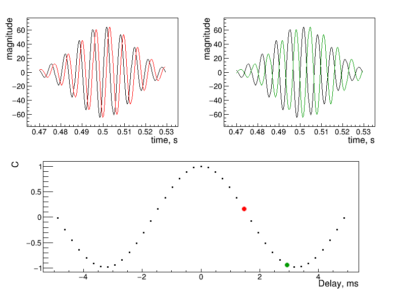
Figure 1: Time-shift effect on the correlation factor due to rigid shifts of a sinusoid with frequency of 153 Hz modulated by a Gaussian envelope. On top row, black curve is the original waveform, red/green (left/right) is the same waveform after a time-shift. On bottom row, values of $C$ calculated applying a time shift (x-axis) to the original waveform. The red and green points refer to the examples in the top row.

We expect a similar behavior in the cases b) and c). In fact, case b) includes a time-shift (introduced by the different values of $\Delta_{k}$) between the original and reconstructed waveforms. In addition to case b), case c) introduces the rotation of the waveform frame ($h_{+}^{\prime}=h_{+}cos(\psi)+h_{\times}sin(\psi)$) which, especially for sinusoidal waveforms (see Fig. 1), is equivalent to a shift in time. Hence, in case c) we have two time-shifts to take into account, one that is the same of case b) and the other due to the difference between original and reconstruted polarization angle The interesting challenge is: do we have a distortion in the signal when we estimate the wrong sky position? Or is an effect due to a rigid shift as in Fig. 1? To answer the question, we include the case d), in which we reconstruct the detector response, the sky localization and also the polarization angle (as in case c) ) and then we add a time shift on $h_{+}$ and $h_{\times}$. The applied time shift is the maximum value of the cross-correlation function of time in which we calculate the cross-correlation between the injected and reconstructed polarization patterns. Hence, we estimate the possible shift among the two waveforms and we calculate the $C$ value after correcting the reconstructed polarizations with this time-shift. In this way we can focus only on possible signal distortions.

III Monte Carlo simulations

As starting point for our tool we decide to take the results obtained by the GW transient signal algorithm in use by the LIGO and Virgo collaborations called coherent Waveburst cWB2008 ; cWB2015 . It is an algorithm to measure energy excesses over the detector noise in the time-frequency domain and combining these excesses coherently among the various detectors. This is performed introducing a maximum likelihood approach to define the ratio among the probability of having a signal in the data over the probability of only noise. This does not need a particular assumption on the expected waveform, making it open to a wide class of transient signals.

The algorithm has recently improved in preparation for the Advanced Detector Era. The main improvement concerns a new method for the estimation of the event parameters which considers assumptions on the polarization state (circular, linear, elliptical, etc…) cWB2015 . This improvement is particularly suited for this work, because, despite it does not calculate directly the two plus and cross polarizations, it is implicitly connected to them through the calculation of the polarization state. The algorithm performances on sky localization and detector response are reported in the previous results PRD2011 ; Reed .

For this work we contemplate a network composed of three interferometers: the two LIGO (L1, Livingston and H1, Hanford) ones and the Virgo (Cascina, Italy) detector, with simulated Gaussian detector noise considering the amplitude spectral density at the design sensitivity LIGO psd ; Virgo psd . Even though most of the noise background in detectors is Gaussian, random instrumental artifacts can make the background far from Gaussian S5 ; S6 ; O1 . The use of Gaussian noise is just the starting point to verify the performances of this new tool. We expect that glitches would affect only the detection confidence and not the reconstruction of the waveforms, as explained in the case of the sky localization Reed . We will check the real behavior of noise when we will handle the data analysis of the three Advanced detectors.

We injected the so-called sine-Gaussian and WhiteNoiseBurst waveforms, which are among the standard tested waveforms for burst searches, respectively representing the limiting case for most simple and complicated morphologies. The former are defined as follows:

$$\begin{split}h_{+}(t)&=h\frac{1+\cos^{2}(\iota)}{2}sin(2\pi tf_{0})exp(-t^{2}/\tau^{2})\\ h_{\times}(t)&=h\cos(\iota)cos(2\pi tf_{0})exp(-t^{2}/\tau^{2})\end{split}$$ (5)

where $f_{0}$ is the central frequency, $\tau$ is related to the waveform quality factor $Q=\sqrt{2}\pi f_{0}\tau$ and the inclination angle $\iota$ is uniformly distributed. For this study we took into account three quality factors $Q=3,9,100$ and three central frequencies: $f_{0}=235,554,1053$ Hz, with source coordinates uniformly distributed in the sky. White Noise Bursts are frequency band limited white noise with a time Gaussian envelope. They have no particular polarization, while SineGaussians have elliptical polarization. To distinguish the various sources of error, we compute the correlation factor (Eq. 4) for the different cases a), b), c) and d). To characterize the algorithm performances, we inject uniformly in the sky at discrete values of the network SNR: 10, 12, 15, 20, 25, 30, 35, where network signal-to-noise ratio (SNR) is defined as the square sum of the ratio of the reconstructed waveform in the frequency domain $(\tilde{h}_{+},\tilde{h}_{\times})$ and the amplitude spectral density $S_{k}(f)$ of each detector $k$: $SNR^{2}=\sum_{k}\int\frac{\tilde{h}_{+}^{2}+\tilde{h}_{\times}^{2}}{S_{k}(f)}df$.

IV Results

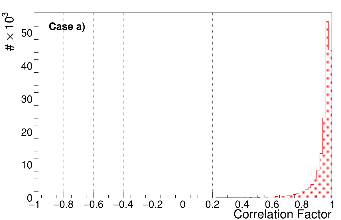
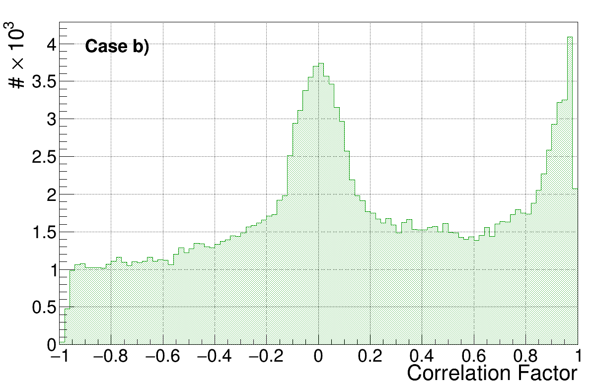
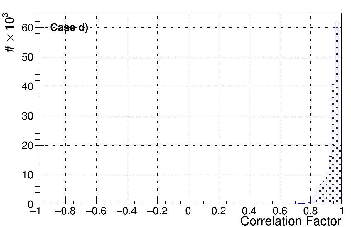
Figure 2: Correlation factor of the plus polarization for injections of a SineGaussian with central frequency of 253 Hz and Q=9 uniformly distributed in the sky and different values of SNR. From left to right, top to bottom: case a), b), c), d).

The aim of the new presented tool is the reconstruction of both polarizations ($+$,$\times$) starting from the results (detector responses, sky localization) of a standard GW transient algorithm. We started the study disentangling the contribution of detector response and sky localization on the estimation of the polarizations. In Fig. 2 we report an example of the $C_{+}$ distribution (Eq. 4) for an elliptical SineGaussian centered at 235 Hz and Q=9 for all the injected SNR. In case a), where we have reconstructed only the detector response, the distribution of the correlation factor is near 1, confirming that the detector response estimation is in agreement with the expected waveforms for the complete set of SNRs. In case b), where we reconstruct both the detector response and the sky positions, it appears a new population centered in 0. Whereas, for case c), where in addition to the information in case b) we reconstruct also the polarization angle, there are three main populations centered respectively to -1, 0, 1. The appearance of these new peaks in b) and c) can be due to two different effects: signal distortion and/or time-shift. As we have explained in Fig. 1, introducing time-shifts lower the value of the Correlation Factor. When we look at case d), where we avoid a possible time shift bringing back the c) waveform to the right time, results display only a remaining distribution around 1, similar to what happens in case a). This answer the question we were posing in the previous section: does a wrong sky localization create distortion of the original signal? Results show that the main effect of estimating the wrong sky position is the introduction of a time-shift between the estimated polarization and the original one, but such distortions on the waveform shape are negligible. The fact that for case b) we do not have so many values of Correlation Factor less than 0 means that the errors from the sky localization cause a time-shift to the reconstructed waveform that is not bigger than a certain value. Thinking in term of phase shift, it is not bigger than a 90 degrees shift. To confirm this last sentence, we compare the results related to case b) considering different injection SNRs (Fig. 3 ) and SineGaussian with different frequencies and same SNR (Fig. 4).

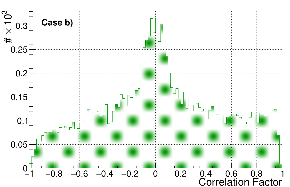
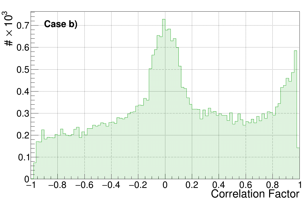
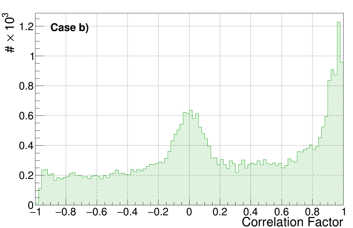
Figure 3: Correlation factor of the plus polarization for case b) for injections of a SineGaussian with central frequency of 253 Hz and Q=9 uniformly distributed in the sky and selected values of SNR. From left to right: SNR=12, 20, 35.

Fig. 3 , where we reported 3 different cases, SNR=12, SNR=20, SNR=35, displays that the widths of the peaks are not different in the three cases. This verifies that the peak at 0 is not related to the SNR, but it gives an hint that could be related to the sample rate. However, the fact that the height of the peaks in 0 and in 1 changes for different SNRs tell us that the sky reconstruction is better for high SNR (as expected). More the SNR is high, less is the number of events affected by a wrong sky localization, which produces a time-shift between the injected and reconstructed waveform polarizations resulting in low values of the Correlation Factor.

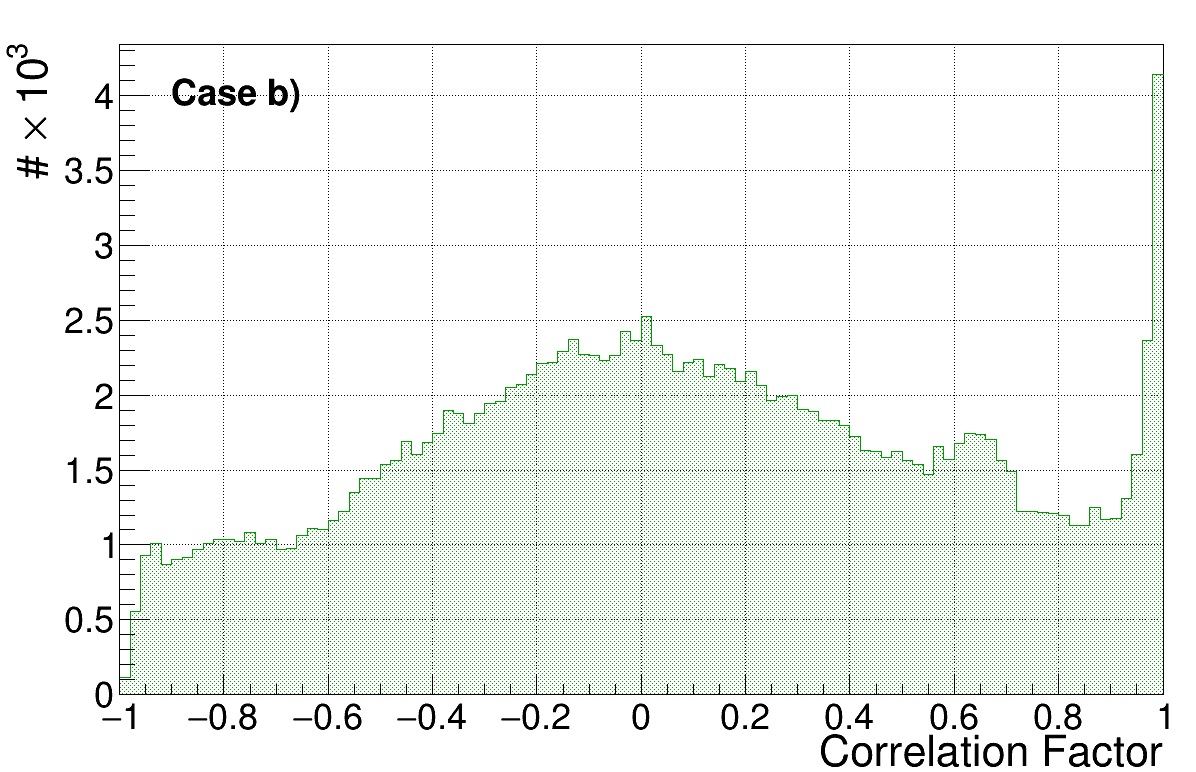
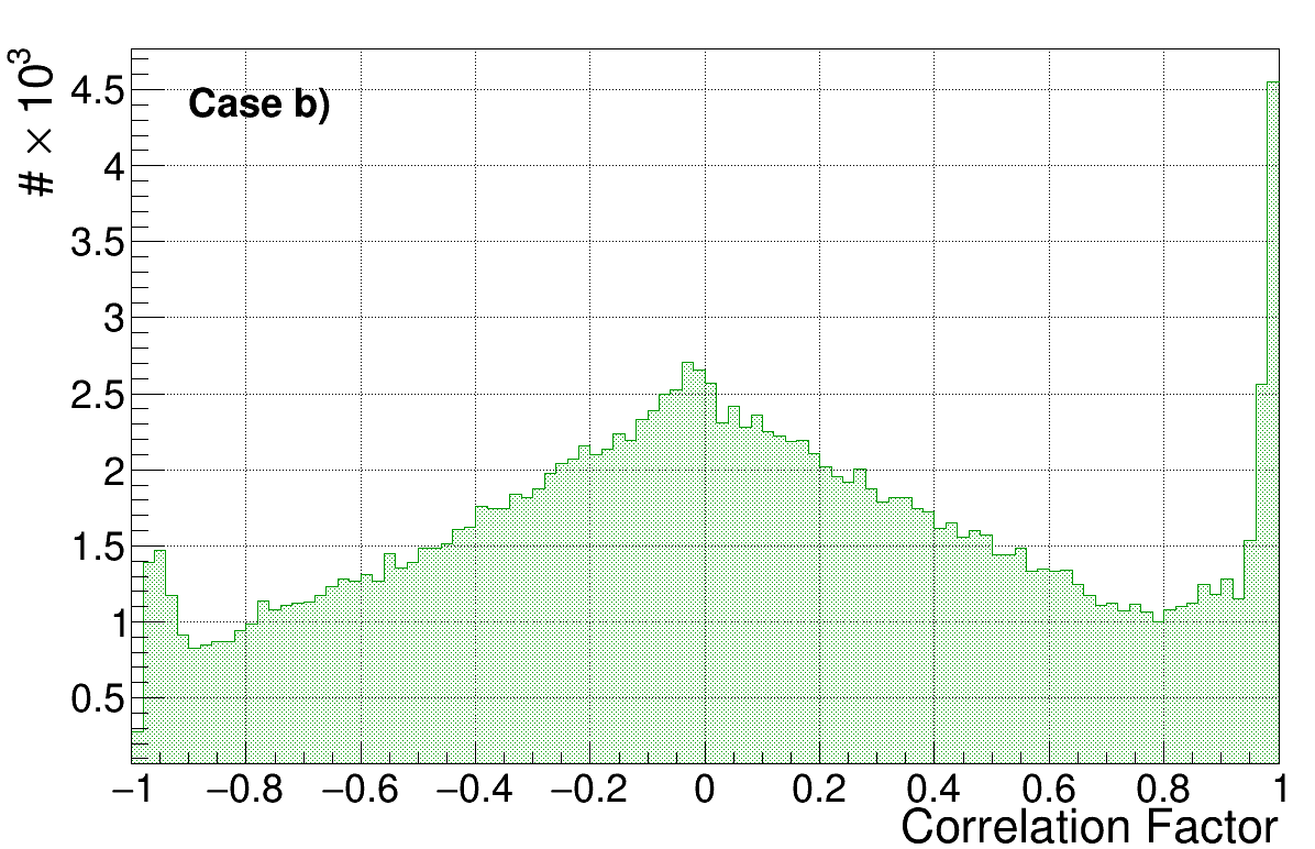
Figure 4: Correlation factor of the plus polarization for case b) for injections of a SineGaussian with Q=9 uniformly distributed in the sky and selected central frequencies. From left to right: central frequency 235, 554, 1053 Hz.

In Fig 4 we show the performances for waveforms at 554 Hz and 1053 Hz of central frequency and compared these with the one of 253 Hz already reported in Fig 2. We can see that the distribution of the results are slightly different, in particular, when the frequency increases, the distribution is not anymore showing the peak in 0, but the values of the correlation factor are more spread in the possible range [-1,1]. The reason is that for this work we adopted the standard SineGaussian definition S5 ; S6 , which groups in the same set waveforms with same quality factor $Q=\sqrt{2}\pi f_{0}\tau$ (see Eq. 5). The quantity Q is mainly related to the number of cycles that characterize the SineGaussian. Therefore, in the same set, given that we have equal cycles but different frequencies, the time duration of the waveforms is inversely proportional to the frequency. Increasing the number of cycles means the possibility to explore more phase shifts between the injected and the reconstructed waveform, when we apply a generic time-shift between the two waveforms. The time-shift between injected and reconstructed depends only on the sky location and, even if the reconstructed sky localization is better when the frequency increases PRD2011 ; Fairhust , such improvement is not enough to contrast the effect of having different number of cycles coming from waveforms at higher frequencies. Increasing the number of cycles means the possibility to explore more phase shifts between the injected and the reconstructed waveform, that shapes the distribution of values of the Correlation Factor.

For case c), instead, the reconstructed polarization angle can differ from the original one in the complete range between 0 and 360 degrees, for this reason it appears the peak at -1. The accumulation point in -1 is always present, for each SNR and frequency, as we can see in the Fig. 5.

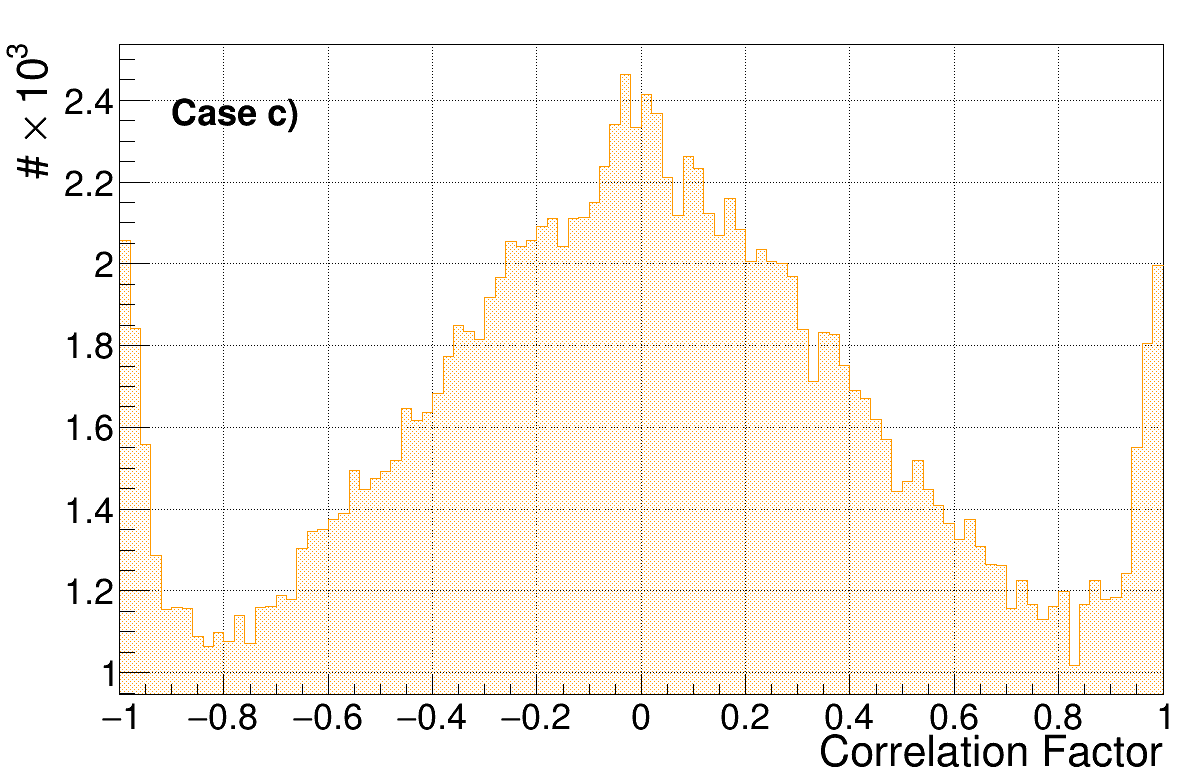
Figure 5: Correlation factor of the plus polarization for case c) for injections of a SineGaussian with Q=9 uniformly distributed in the sky and selected central frequencies. From left to right: central frequency 235, 554, 1053 Hz.

To confirm this we tried the case of injected sky position and reconstructed polarization angle (we call this case e) and we report the result for the SineGaussian at central frequency of 235 Hz and Q=9 in Fig 6 (but for other waveforms results are similar). The Fig. 6 shows that the peak at -1 is still present, validating the fact that it is related to the wrong estimation of the polarization angle (moreover the peak at 0 is disappeared).

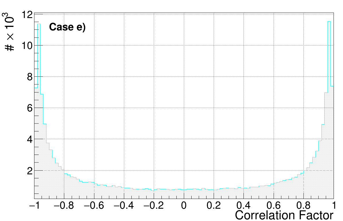
Figure 6: Correlation factor of the plus polarization for case c) for injections of a SineGaussian with central frequency of 253 Hz and Q=9 uniformly distributed in the sky and all the tested SNR .

On Fig. 7(a) we estimate, from the distribution of Fig. 2, the median value. The shaded regions refer to the values for which we obtain the percentile between 30% and 70%. On 7(b) we have the same results for a WhiteNoiseBurst. We see that for each case (from a) to d)) a waveform like a SineGaussian shows in general a median nearer to the optimal value of 1 than a waveform like a WhiteNoiseBurst. These waveforms show a time-frequency representation which involves a greater number of pixels. Having more pixels naturally increases the noise contribution to the waveform reconstruction. This easily explains the reason why performances for SineGaussian are better than for WhiteNoiseBurst, given that it is possible to characterize the first ones with less time-frequency pixels. Indeed, for the SineGaussian case, results are independent of the tested SNR. Since a decrease in the SNR values produces a contamination of the noise in the performances, we chose a network SNR=10 (detector SNR$\approx 10/\sqrt{3}<6$) as a reasonable threshold for a candidate event, as explained and done before for searches in burstPaper .

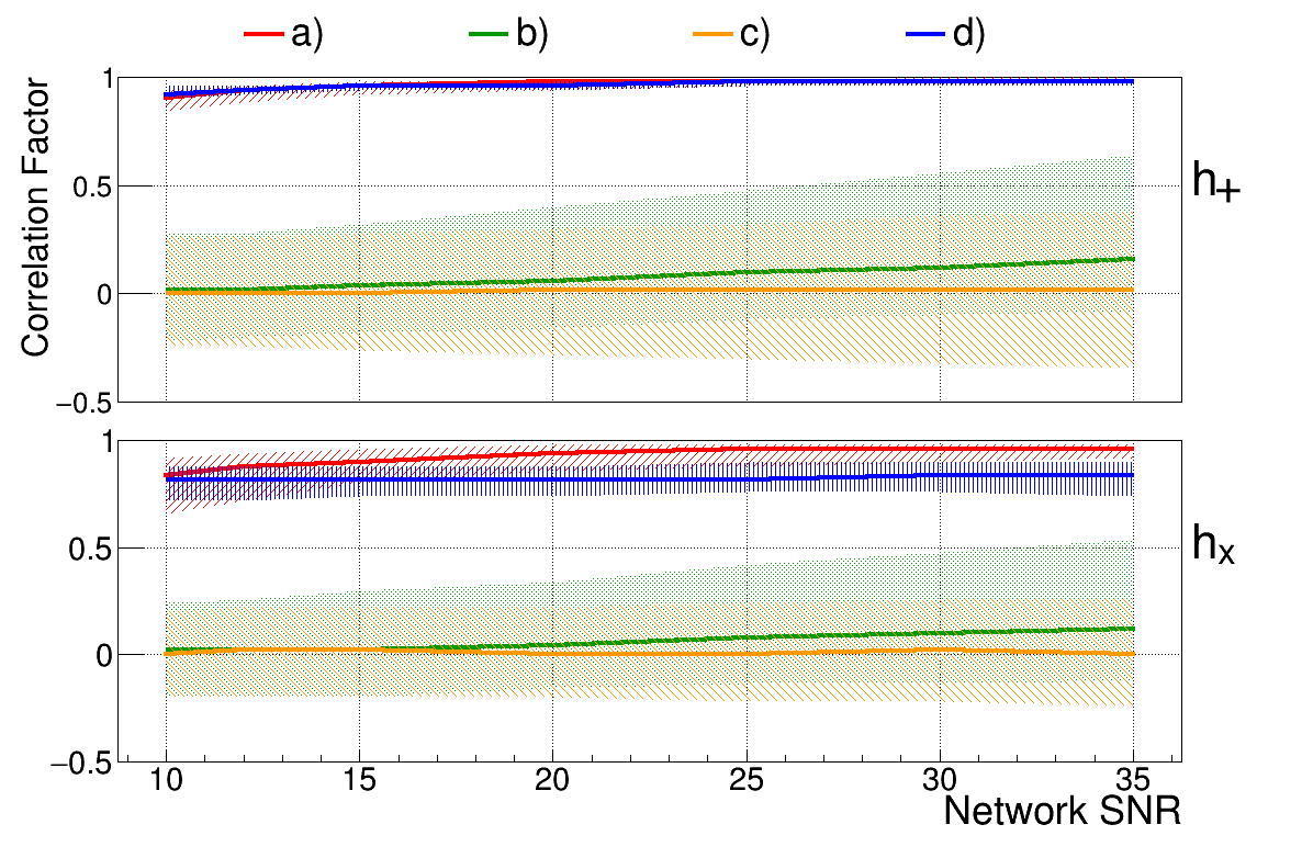
(a) SineGaussian with central frequency of 253 Hz and Q=9

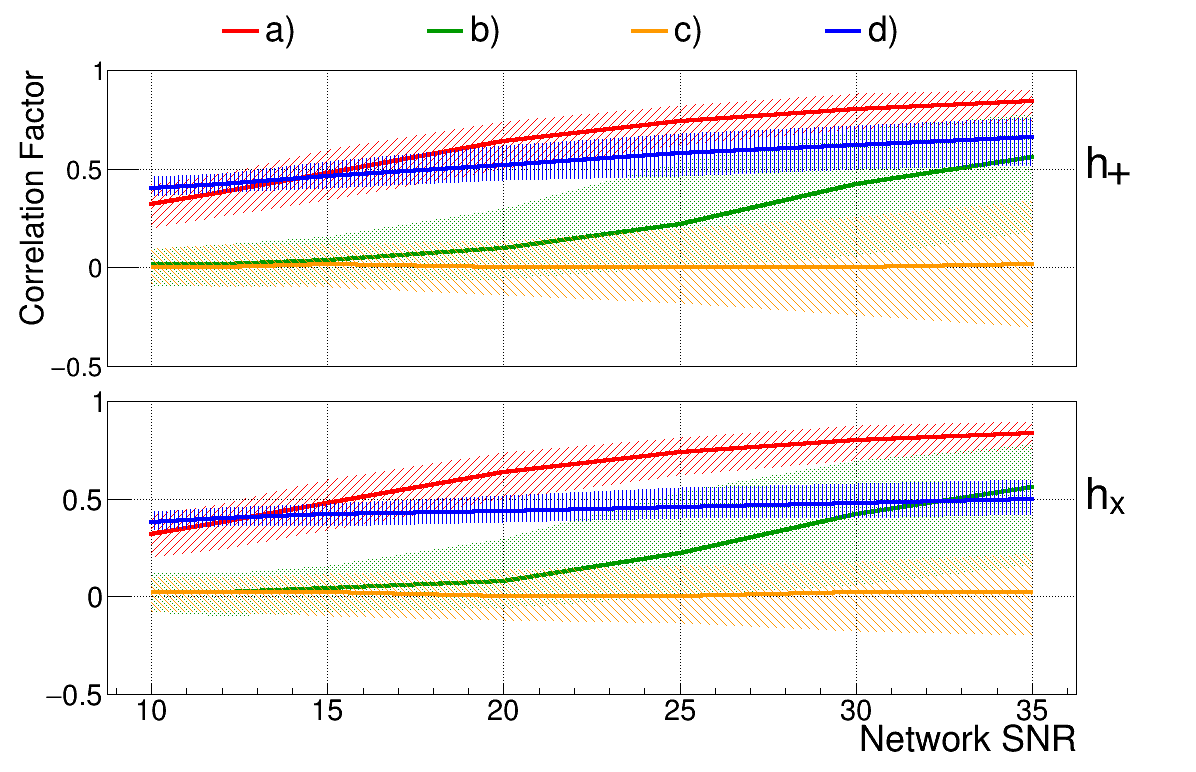
(b) WhiteNoiseBurst with frequency range (250,350) Hz and duration of 100ms.

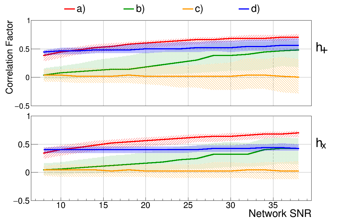
(c) Binary black holes coalescence with single component masses between 15 and 25 solar masses

Figure 7: Median (lines) and 30%-70% percentile (colored regions) of Correlation Factor for the plus (top) and cross (bottom) polarization for injections uniformly distributed in the sky as a function of the injected SNR. Colours refer to cases labelled in the text as a) (red), b) (green), c) (orange), d) (blue).

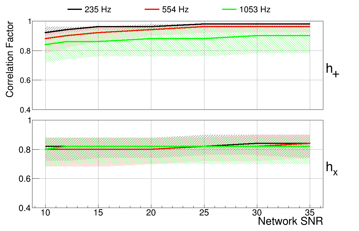
(a) SineGaussian with Q=9 and central frequency at 235 Hz (black), 554 Hz (red), 1053 Hz (green).

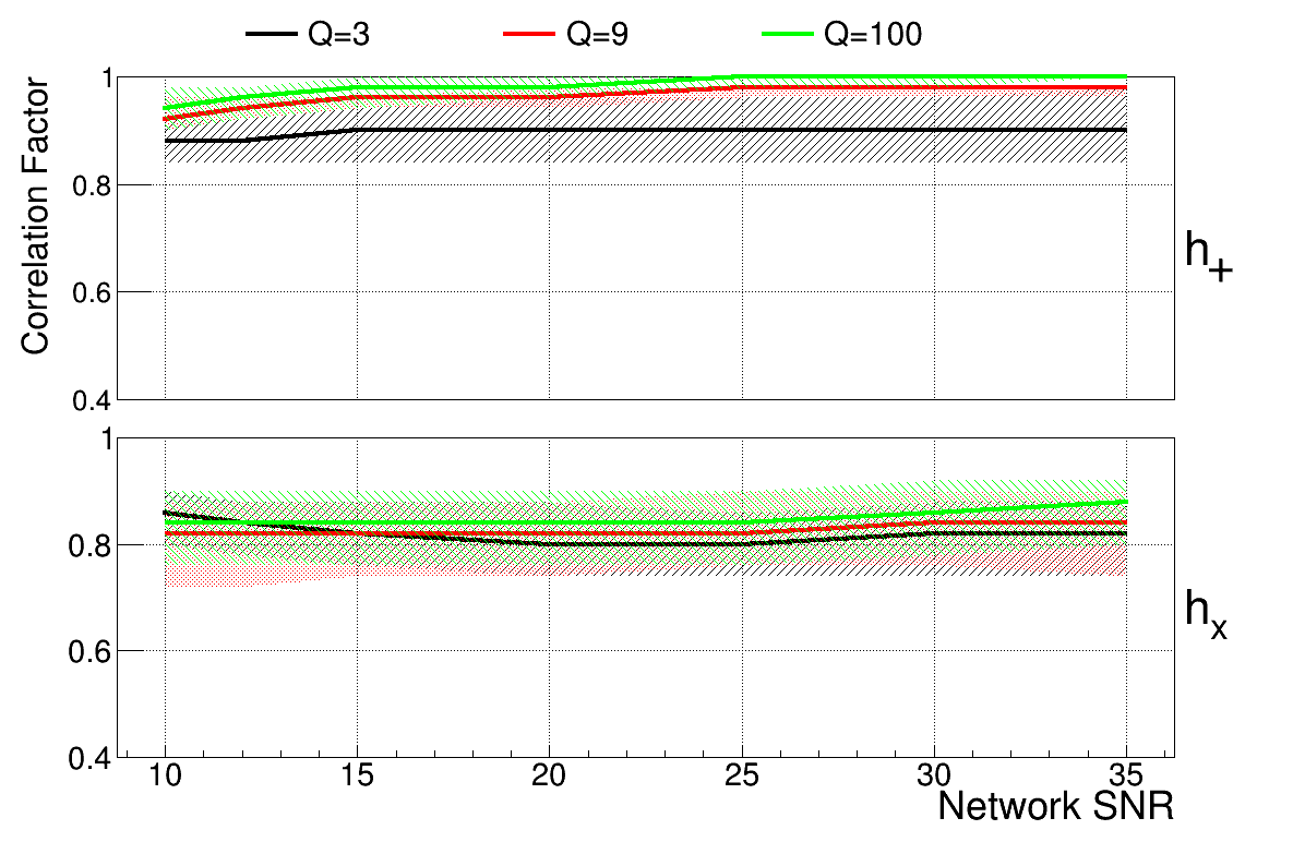
(b) SineGaussian with central frequency = 235 Hz and Q=3 (black), Q=9 (red) , Q=100 (green).

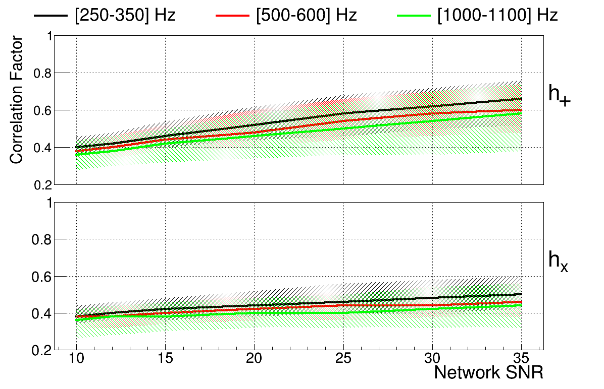
(c) WhiteNoiseBurst with bandwidth (250,350) Hz (black), (500,600) Hz (red) and (1000,1100) Hz (green).

Figure 8: Median (lines) and 30%-70% percentile (colored regions) of Correlation Factor for the plus (top) and cross (bottom) polarization for different signals for the d) case. The y-axis shows what is the correlation factor value for which the 50% (lines) and the 30%-70% percentiles of the recovered waveforms have bigger cross correlation.

IV.1 Transient signals

In this paper we are interested in the reconstruction of the waveform shape with the aim to estimate the characteristics of the generating source from the waveform itself. Given the purpose, we want to focus on eventual signal distortions in the reconstructed polarization patterns. Since in real analysis we do not know the true quantities, we should focus on case c). However, as already discussed and shown in Fig. 2 for this case the correlation factor $C$ describes both the effects of signal distortion and time-shift. Hence, in the following we consider the case d) because it is connected only to the distortion and not to any eventual time-shift applied to the signal.
In Fig. 8(a) we report the comparison of SineGaussian with the same Q=9 but at the different central frequencies. We can see that performances are better for plus polarization, $(+)$. This is probably because for most of the injection the $(+)$ plus polarization has higher energy than the cross one, $(\times)$. Indeed there are negligible differences for the $(\times)$ cross polarization among the three frequencies, but for the plus polarization $(+)$ we can see that performances are better for lower frequencies, probably due to the fact that these oscillations are less separated in time. This is confirmed also in Fig. 8(b) where we show the comparison for SineGaussian with same central frequency but different Q. We see that when Q increases, performances are better, because waveform’s bandwidth is narrow and the time-frequency representation involves less pixels.

Similar results for WhiteNoiseBurst are shown in Fig. 8(c), where the performances are better for lower frequencies. Moreover, for these waveforms the performances are slightly worse, with respect to SineGaussian. Indeed, the WhiteNoiseBurst signals are more widespread in the time-frequency domain than the Sine-Gaussian, which makes more difficult to accurately reconstruct the complete waveform. As already shown (Fig. 7(b)), for these waveforms the contribution to the errors coming from the detector response estimation is more important than the SineGaussian.

IV.2 Compact Binary Coalescence

For completeness, we also tested the algorithm on a set of signals coming from the coalescence of binary black hole systems. The first detections of gravitational waves were generated by the merge of two black holes that are the most cataclysmic events in nature. In such systems two black holes combine to form a single one, emitting a strong gravitational wave. In our simulations we consider binary black hole systems with single masses between 15 and 25 solar masses and uniform spin distribution between 0 and 0.9. These are the same waveforms used in Reed , where the cWB performances on sky localization have already been reported. Waveforms have been injected up to 4 Gpc, using a uniform distribution in volume. We are not considering any cosmological evolution, so in the previous values we are referring to masses in the source frames and luminosity distance. The reconstructed events have been collected in bins of network SNR, each bin has width equal to 2. To be homogeneous with the results of the other waveforms we consider a SNR range from 8 to 38. Results from these tests are reported in Fig. 7(c). The results are similar to the case of White Noise Bursts in Fig. 7(b). Indeed the signals belonging to these two classes involve a greater number of pixels in the time-frequency domain. This increases the noise contribution on the waveform estimation, which makes more difficult to accurately reconstruct the complete waveform.

V Conclusion

We have tested a new algorithm for the inverse solution as from the information given by a non-template search and reconstructed the original waveform polarization. This approach is the first attempt to use and verify the accuracy of the tool. Assuming the detectors at the design sensitivity and Gaussian noise, results show a reliable reconstruction of both plus $(+)$ and cross $(\times)$ polarizations, even for low injected values of SNR.
Through the disentanglement of the various error contributions, we have shown that the main effect is due to the detector response. In fact, the correction caused by the sky position is mainly a time-shift of the signal proper time, but no significant distortion appears on the original waveform, as seen in Fig. 2.
We are working to obtain further improvements and refinement of the reconstruction by reducing the contribution of the noise in the detector response estimation. In future works we propose to verify if real detector noise gives comparing results and to study the effect of the matrix deficiency, for instance applying the approach proposed in Rakhmanov . This tool does not rely on a specific pipeline, hence, it can be applied to any algorithm that provides information of the detector response and sky location. It would be interesting to apply this approach to detected events of Advanced LIGO and Virgo in the future observational runs. For events detected with template searches, it would be straightforward to compare the polarizations obtained with this method with the ones given by the template. This would allow to check the performances of this approach with the best matching, but also can give hints on possible variations of the real signal from the template itself. For events detected with un-modeled algorithms, reconstructing the polarizations would be the first step to understand the generating process, other than the astrophysical progenitor.

VI Acknowledgments

The authors gratefully acknowledge the support of the research by the Italian Istituto Nazionale di Fisica Nucleare and the Max-Planck-Society, and the State of Niedersachsen/Germany. They also gratefully acknowledge the support of L’Oréal Italia For Women in Science.

References

- (1) A. Einstein, Sitzungsber. K. Preuss. Akad. Wiss. 1 688, 1916.
- (2) A. Einstein, Sitzungsber. K. Preuss. Akad. Wiss. 1 154, 1918.
- (3) R. A. Hulse and J. H. Taylor, Astrophys. J. 195 L51, 1975.
- (4) H. Taylor and J. M. Weisberg, Astrophys. J., 253, 908 (1982)
- (5) J. Aasi et al, Class. Quantum Grav. 32, 11, 2015
- (6) T Accadia, et al., Journal of Instrumentation 7 P03012, 2012
- (7) J. Abadie et al., Phys. Rev. D 85 122007, 2012.
- (8) J. Abadie et al., Phys. Rev. D 85 082002, 2012.
- (9) J. Abadie et al., Phys. Rev. D 90 062010, 2014.
- (10) J. Aasi et al., Phys. Rev. Lett 113 231101, 2014.
- (11) Grote H et al., Class. Quantum Grav. 27 084003, 2010.
- (12) J. Abadie et. al, Class. Quantum Grav. 32 074001, 2015.
- (13) F. Acernese, et. al, Class. Quantum Grav. 32 024001, 2015.
- (14) G. M. Harry. Class. Quant. Grav., 27 084006 (2010).
- (15) The Virgo Collaboration, Advanced Virgo Technical Design Report, 2012. [VIR-0128A-12].
- (16) Y. Aso et al., Phys. Rev. D 88 043007, 2013.
- (17) K. Somiya, Class. Quantum Grav. 29 124007, 2012.
- (18) B. Iyer, et al., LIGO-India Tech. rep. (2011), https://dcc.ligo.org/LIGO-M1100296/public
- (19) B. P. Abbott et al., PRL 116, 061102, 2016.
- (20) S. Fairhust, Classical Quantum Gravity 28, 105021, 2011
- (21) B. P. Abbott et al., PRD 93, 122004, 2016.
- (22) B. P. Abbott et al., PRD 93, 122003, 2016.
- (23) S. Klimenko et al., Classical Quantum Gravity 25, 114029, 2008.
- (24) S. Klimenko et al., Phys. Rev. D 93, 043007, 2016.
- (25) B. P. Abbott et al., Phys. Rev. Lett. 116 221101, 2016.
- (26) B. P. Abbott et al., Phys. Rev. Lett. 116 241102, 2016.
- (27) B. P. Abbott et al., Phys.Rev.Lett. 116, 241103, 2016.
- (28) B. P. Abbott et al., Phys.Rev.Lett. 118, 221101, 2017.
- (29) B. P. Abbott et al., arXiv:1711.05578
- (30) B. P. Abbott et al., Phys.Rev. X6 no.4, 041015, 2016
- (31) B. P. Abbott et al., Phys.Rev.Lett. 119, 141101, 2017
- (32) B. P. Abbott et al., Phys.Rev.Lett. 119, 161101, 2017
- (33) B. P. Abbott et al., Astrophys.J. 848, no. 2, L13, 2017
- (34) B. P. Abbott et al., Nature, 10.0138/nature24471, 2017
- (35) B.P. Abbott (Caltech) et al., Astrophys.J. 818 no.2, L22, 2016
- (36) J. Abadie et al., Phys. Rev. D 81 102001, 2010.
- (37) S. Chatterji, A. Lazzarini, L. Stein, P. Sutton, A. Searle and M. Tinto, Phys. Rev. D 74 082005, 2006.
- (38) W. G. Anderson, P. R. Brady, J. D. E. Creighton and E. E. Flanagan, Phys. Rev. D 63 042003, 2001.
- (39) L. Wen and B. Schutz, Class. Quantum Grav. 22 S1321, 2005.
- (40) L. Cadonati, Class. Quantum Grav. 21 S1695 2004.
- (41) N. Cornish and T. Littenberg,, Class. Quantum Grav. 32, 13 2015.
- (42) B. S. Sathyaprakash and B. F. Schutz, Living Reviews in Relativity, 12(2), 2009.
- (43) S. Klimenko et al, Phys.Rev.D 72, 122002, 2005.
- (44) S. Klimenko et al, Phys. Rev. D 83, 102001, 2011.
- (45) R. Essick et al., The Astrophysical Journal, 800, 2
- (46) M. Rakhmanov Class. Quantum Grav. 23, S673-S685, 2006.
- (47) https://dcc.ligo.org/LIGO-T0900288/public.
- (48) https://tds.ego-gw.it/ql/?c=6589.
- (49) B. P. Abbott et al., Phys. Rev. D 95 042003, 2017.